Quantum ESPRESSO

Notes on parallel computing

Parallel programming paradigms

Most modern electronic-structure code use one of the following approaches, or acombination of them:

• MPI (Message Passing Interface) parallelizationMany processes are executed in parallel, one per processor, accessing their ownset of variables. Access to variables on another processor is achieved via explicitcalls to MPI libraries.

• OpenMP parallelizationA single process spawns sub-processes (or “threads”) on other processors thatcan access and process the variables of the code. Achieved with compilerdirectives and/or via call to “multi-threading” libraries like Intel MKL or IBMESSL.

Quantum ESPRESSO exploits both MPI and OpenMP parallelization; the formeris well-established, the latter is quickly stabilizing.

Comparison of parallel programming paradigms

MPI parallelization:

+ Portable to all architectures (as long as MPI libraries exist)

+ Can be very efficient (as long as MPI libraries are)

+ Can scale up to a large number of processors

– Requires significant code reorganization and rewriting

OpenMP parallelization:

+ Relatively easy to implement: requires modest code reorganization and rewriting

– Not very efficient: doesn’t scale on more than a few processors. Interesting formulti-core CPU’s or, in combination with MPI, for large parallel machines basedon multi-core CPU’s (e.g.: IBM BlueGene).

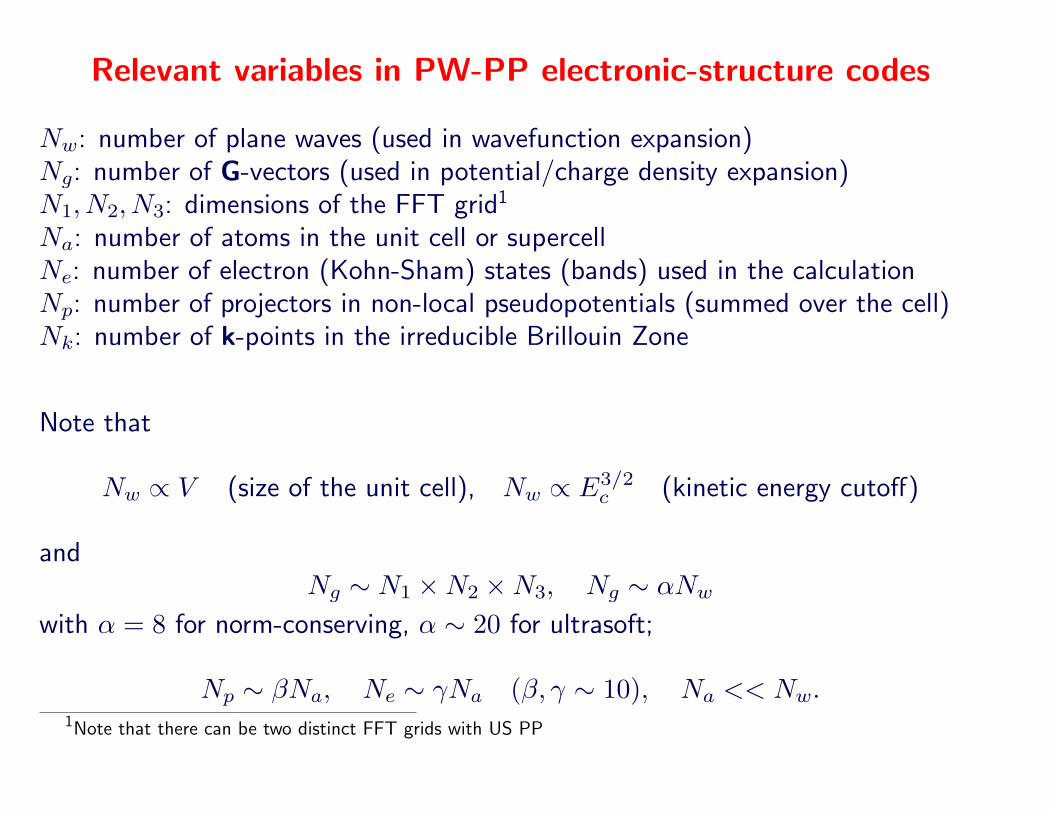
Relevant variables in PW-PP electronic-structure codes

Nw: number of plane waves (used in wavefunction expansion)Ng: number of G-vectors (used in potential/charge density expansion)N1, N2, N3: dimensions of the FFT grid1

Na: number of atoms in the unit cell or supercellNe: number of electron (Kohn-Sham) states (bands) used in the calculationNp: number of projectors in non-local pseudopotentials (summed over the cell)Nk: number of k-points in the irreducible Brillouin Zone

Note that

Nw ∝ V (size of the unit cell), Nw ∝ E3/2c (kinetic energy cutoff)

andNg ∼ N1 ×N2 ×N3, Ng ∼ αNw

with α = 8 for norm-conserving, α ∼ 20 for ultrasoft;

Np ∼ βNa, Ne ∼ γNa (β, γ ∼ 10), Na << Nw.1Note that there can be two distinct FFT grids with US PP

Time-consuming steps in PW-PP electronic-structure codes

• Calculation of density, n(r) =∑|ψ(r)|2:

FFT + linear algebra (matrix-matrix multiplication)

• Calculation of potential, V (r) = Vxc[n(r)] + VH[n(r)]:FFT + operations on real-space grid

• Iterative diagonalization (SCF) / electronic force (CP) calculation, Hψ products:FFT + linear algebra (matrix-matrix multiplication)

• Subspace diagonalization (SCF) / Iterative orthonormalization of Kohn-Shamstates (CP): diagonalization of Ne×Ne matrices + matrix-matrix multiplication

Basically: most CPU time spent in linear-algebra operations, implemented in BLASand LAPACK libraries, and in FFT

Memory-consuming arrays in PW-PP electronic-structurecodes

• Wavefunctions (Kohn-Sham orbitals):at least nk arrays (at least 2 for CP) of size Nw ×Ne, plus a few more copiesused as work space. If nk > 1, arrays can be stored to disk and used one at thetime, thus reducing memory usage, at the price of increased disk I/O

• Charge density and potential:several vectors with dimension Ng (in G-space) or Nr = N1 × N2 × N3 (inR-space) each

• Pseudopotential projectors:a Nw ×Np array containing βi(G)

• Miscellaneous Matrices:Ne×Ne arrays containing 〈ψi|ψj〉 products used in subspace diagonalization oriterative orthonormalization; Ne ×Np arrays containing 〈ψi|βj〉 products

Required actions for effective parallelization of PW-PPelectronic-structure codes

• Balance load:all processors should have the same load as much as possible

• Reduce communications to the strict minimum:communication is typically slower or much slower than computation!

• Distribute all memory that grows with the size of the cell:if you don’t, you will run out of memory for large cells

• Distribute all computation that grows with the size of the cell:if you don’t, sooner or later non-parallelized calculations will take most of thetime (a practical demonstration of Amdhal’s law)

The solution currently implemented in Quantum ESPRESSO introduces severallevels of parallelization.

Parallelization level 1

• Image parallelization:Currently implemented only for NEB, but there are other cases where it couldbe useful. Images, i.e. points in the coordinate space, are distributed acrossnimage groups of CPUs. Example for 64 processors divided into nimage = 4groups of 16 processors each:

mpirun -np 64 pw.x -nimage 4 -inp input file

+ potentially linear CPU scalability, limited by number of images:nimage must be a divisor of the number of NEB images

+ very modest communication requirements

o load balancing fair to good: unlikely that all images take the same CPU

– memory usage does not scale at all!

Good when usable, especially if the communication hardware is not so fast

Parallelization level 2

• k-point parallelization:k-points are distributed (if more than one) among npool pools of CPUs. Examplefor 16 processors divided into nimage = 4 image groups of npool = 4 pools of 4processors each:

mpirun -np 64 pw.x -nimage 4 -npool 4 -inp input file

+ potentially linear scalability, limited by number of k-points:npool must be a divisor of Nk

+ modest communication requirements

o load balancing fair to good

– memory usage does not scale in practice

Good if one has k-points, especially if the communication hardware is not so fast

Parallelization level 3

• Plane-wave parallelization:wave-function coefficients are distributed among nPW CPUs so that each CPUworks on a subset of plane waves. The same is done on real-space grid points.This is the default parallelization scheme if other parallelization levels are notspecified. In the example above:

mpirun -np 64 pw.x -nimage 4 -npool 4 -inp input file

plane-wave parallelization is performed on groups of 4 processors.

+ high scalability of memory usage: the largest arrays are all distributed+ good load balancing among different CPUs if nPW is a divisor of N3

+ excellent scalability, limited by the real-space 3D grid to nPW ≤ N3

– heavy and frequent intra-CPU communications, mainly in the 3D FFT

Best choice overall, if one has sufficiently fast communication hardware

Parallelization level 4

• linear-algebra parallelization:distribute and parallelize matrix diagonalization and matrix-matrixmultiplications needed in iterative diagonalization (PWscf) or orthonormalization(CP). Introduces a linear-algebra group of ndiag processors as a subset of theplane-wave group. ndiag = m2, where m is an integer such that m2 ≤ nPW .Not used by default (changed in new version). Should be set using the -ndiagor -northo command line option, e.g.:

mpirun -np 64 pw.x -ndiag 25 -inp input file

+ RAM is efficiently distributed: removes a major bottleneck in large systems+ Increases speedup in large systemso Scaling tends to saturate: testing required to choose optimal value of ndiag

Home-made parallel algorithms are supplied, but ScaLAPACK works much better forserious calculations. Useful in large systems, when the RAM and CPU requirementsof linear-algebra operations become a sizable share of the total.

Parallelization level 5

• task group parallelization:each plane-wave group of processors is split into ntask task groups of nFFT

processors, with ntask × nFFT = nPW ; each task group takes care of the FFTover Ne/nt states. Used to extend scalability of FFT parallelization. Not setby default. Example for 4096 processors divided into nimage = 8 images ofnpool = 2 pools of nPW = 256 processors, divided into ntask = 8 tasks ofnFFT = 32 processors each; subspace diagonalization performed on a subgroupof ndiag = 144 processors :

mpirun -np 4096 pw.x -nimage 8 -npool 2 -ntg 8 -ndiag 144 ...

Allows to extend scaling when the PW parallelization saturates: definitely neededif you want to run on more than ∼ 100 processors.

Parallelization level 6

• OpenMP parallelization:

explicit (with directives) parallelization of FFT is activated at compile timewith preprocessing flag; currently implemented only for ESSL and FFTW.Requires an OpenMP-aware compiler,implicit (with libraries) parallelization with OpenMP-aware libraries: currentlyonly ESSL and MKL

+ Extends scaling

- Danger of MPI-OpenMP conflicts!

To be used on large multicore machines (e.g. IBM BlueGene), in which severalMPI instances running on the same node do not give very good performances.

Summary of parallelization levels in Quantum ESPRESSO

group distributed quantities communications performances

image NEB images very low linear CPU scaling,fair to good load balancing;does not distribute RAM

pool k-points low almost linear CPU scaling,fair to good load balancing;does not distribute RAM

plane- PW, G-vector coefficients, high good CPU scaling,wave R-space FFT arrays good load balancing,

distributes most RAM

task FFT on electron states high improves load balancinglinear- subspace hamiltonians very high improves scaling,algebra and constraints matrices distributes more RAM

OpenMP FFT, libraries intra-node extends scaling onmulticore machines

(Too) Frequently Asked Question(that qualify you as a parallel newbie)

• How many processors can (or should) I use?It depends!

• It depends upon what??

– Upon the kind of physical system you want to study: the larger the systems,the larger the number of processors you can or should use

– Upon the factor driving you away from serial execution towards parallelexecution: not enough RAM, too much CPU time needed, or both? If RAMis a problem, you need plane-wave parallelization

– Upon the kind of machine you have: plane-wave parallelization is ineffectiveon more than 4÷8 processors connected with cheap communication hardware

• So what should I do???You should benchmark your job with different numbers of processors, pools,image, task, linear algebra groups, taking into account the content of previousslides, until you find a satisfactory configuration for parallel execution.

Compiling and running in parallel

• Compilation: if you have a working parallel environment (compiler / libraries),configure will detect it and will attempt a parallel compilation by default.Beware serial-parallel compiler conflicts, signaled by lines like

WARNING: serial/parallel compiler mismatch detected

in the output of configure. Check for the following in make.sys:

DFLAGS= ...-D PARA -D MPI ...MPIF90=mpif90 or any other parallel compiler

For MPI-OpenMP parallelization, use./configure --enable-openmpverify the presence of -D OPENMP in DFLAGS

If configure doesn’t detect a parallel machine as such, your parallelenvironment is either disfunctional (nonexistent or incomplete or not workingproperly) or exotic (in nonstandard locations or for strange machines) .

Compiling and running in parallel (2)

• Execution: beware the syntax! the total number of processor is sometimesan option of mpirun / mpiexec / whatever applies, sometimes it is set bythe batch queueing system; -nimage, -npool, -ndiag, -ntg are options ofQuantum ESPRESSO executables and should follow them.

On some machines, you may need to supply input data using QuantumESPRESSO option -inp filename; you may also need to supply optionalarguments via “mpirun -args ’optional-arguments’”

Be careful not to make heavy I/O via NFS. Write to either a parallel filesystem (found only on expensive machines) or to local disks. In the latter case,check that all processors can access pseudo dir and outdir. PWscf: useoption wf collect to collect final data files in a single place; consider usingoption disk io to reduce I/O to the strict minimum.

Mixed MPI-OpenMP parallelization should be used ONLY on machines (e.g.BlueGene) that allow you to control how many MPI processes run on a givennode, and how many OpenMP threads.

Scalability for “small” systems

Typical speedup vs number of processors:

128 Water molecules (1024 electrons) in acubic box 13.35 A side, Γ point.PWscf code on a SP6 machine, MPI only.ntg=1 parallelization on plane waves onlyntg=4 also on electron states

Scalability for “medium-size” systems

PSIWAT: Thiol-covered gold surfaceand water, 4 k−points, 10.59 ×20.53× 32.66 A3 cell, 587 atoms, 2552electrons. PWscf code on CRAY XT4,parallelized on plane waves, electronstates, k−points. MPI only.

CNT(1): nanotube functionalized withporphyrins, Γ point, 1532 atoms, 5232electrons. PWscf code on CRAY XT4,parallelized on plane waves and electronstates, MPI only.

CNT(2): same system as for CNT(1).CP code on a Cray XT3, MPI only.

3D parallel distributed FFT is the main bottleneck. Additional parallelization levels(on electron states, on k−points if available) allow to extend scalability.

Mixed MPI-OpenMP scalability

Fragment of an Aβ-peptide in watercontaining 838 atoms and 2312electrons in a 22.1×22.9×19.9 A3 cell,Γ-point. CP code on BlueGene/P, 4processes per computing node.

Two models of graphene on Ir surfaceon a BlueGene/P using 4 processes percomputing node. Execution times in s,initialization + 1 self-consistency step.

N cores T cpu (wall) T cpu (wall)443 atoms 686 atoms

16384 740(772) 2861 (2915)32768 441(515) 1962 (2014)65536 327(483) 751 (1012)

(the large difference between CPU andwall time is likely due to I/O)