quantum field theory i - uni-heidelberg.deduo/skripten/...quantum field theory i by prof. michael g....
TRANSCRIPT
Quantum Field Theory I
by Prof. Michael G. Schmidt
24 October 2007
Processed and LATEX-ed by Olivier Tieleman
Supported byAdisorn Adulpravitchai and Jenny Wagner
This is a first version of the lecture notes for professor Michael Schmidt’scourse on quantum field theory as taught in the 2006/2007 winter semester.Comments and error reports are welcome; please send them to:
o.tieleman at students.uu.nl

2

Contents
1 Introduction 51.1 Particle field duality . . . . . . . . . . . . . . . . . . . . . . . 51.2 Short repetition of QM . . . . . . . . . . . . . . . . . . . . . . 5
1.2.1 Mechanics . . . . . . . . . . . . . . . . . . . . . . . . 61.2.2 QM States . . . . . . . . . . . . . . . . . . . . . . . . 61.2.3 Observables . . . . . . . . . . . . . . . . . . . . . . . . 71.2.4 Position and momentum . . . . . . . . . . . . . . . . . 71.2.5 Hamilton operator . . . . . . . . . . . . . . . . . . . . 8
1.3 The need for QFT . . . . . . . . . . . . . . . . . . . . . . . . 91.4 History . . . . . . . . . . . . . . . . . . . . . . . . . . . . . . 121.5 Harmonic oscillator, coherent states . . . . . . . . . . . . . . 12
1.5.1 Classical mechanics . . . . . . . . . . . . . . . . . . . . 121.5.2 Quantization . . . . . . . . . . . . . . . . . . . . . . . 131.5.3 Coherent states . . . . . . . . . . . . . . . . . . . . . . 14
1.6 The closed oscillator chain . . . . . . . . . . . . . . . . . . . . 181.6.1 The classical system . . . . . . . . . . . . . . . . . . . 181.6.2 Quantization . . . . . . . . . . . . . . . . . . . . . . . 191.6.3 Continuum limit . . . . . . . . . . . . . . . . . . . . . 211.6.4 Ground state energy . . . . . . . . . . . . . . . . . . . 23
1.7 Summary . . . . . . . . . . . . . . . . . . . . . . . . . . . . . 241.8 Literature . . . . . . . . . . . . . . . . . . . . . . . . . . . . . 24
2 Free EM field, Klein-Gordon eq, quantization 272.1 The free electromagnetic field . . . . . . . . . . . . . . . . . . 27
2.1.1 Classical Maxwell theory . . . . . . . . . . . . . . . . 272.1.2 Quantization . . . . . . . . . . . . . . . . . . . . . . . 302.1.3 Application: emission, absorption . . . . . . . . . . . . 312.1.4 Coherent states . . . . . . . . . . . . . . . . . . . . . . 32
2.2 Klein-Gordon equation . . . . . . . . . . . . . . . . . . . . . . 322.2.1 Lagrange formalism for field equations . . . . . . . . . 322.2.2 Wave equation, Klein-Gordon equation . . . . . . . . . 352.2.3 Quantization . . . . . . . . . . . . . . . . . . . . . . . 362.2.4 The Maxwell equations in Lagrange formalism . . . . 37
3
4 CONTENTS
3 The Schrodinger equation in the language of QFT 413.1 Second Quantization . . . . . . . . . . . . . . . . . . . . . . . 41
3.1.1 Schrodinger equation . . . . . . . . . . . . . . . . . . . 413.1.2 Lagrange formalism for the Schrodinger equation . . . 423.1.3 Canonical quantization . . . . . . . . . . . . . . . . . 43
3.2 Multiparticle Schrodinger equation . . . . . . . . . . . . . . . 453.2.1 Bosonic multiparticle space . . . . . . . . . . . . . . . 453.2.2 Interactions . . . . . . . . . . . . . . . . . . . . . . . . 473.2.3 Fermions . . . . . . . . . . . . . . . . . . . . . . . . . 48
4 Quantizing covariant field equations 514.1 Lorentz transformations . . . . . . . . . . . . . . . . . . . . . 514.2 Klein-Gordon equation for spin 0 bosons . . . . . . . . . . . . 52
4.2.1 Klein-Gordon equation . . . . . . . . . . . . . . . . . . 524.2.2 Solving the Klein-Gordon equation in 4-momentum
space . . . . . . . . . . . . . . . . . . . . . . . . . . . 534.2.3 Quantization: canonical formalism . . . . . . . . . . . 554.2.4 Charge conjugation . . . . . . . . . . . . . . . . . . . . 58
4.3 Microcausality . . . . . . . . . . . . . . . . . . . . . . . . . . 594.4 Nonrelativistic limit . . . . . . . . . . . . . . . . . . . . . . . 60
5 Interacting fields, S-matrix, LSZ 635.1 Non-linear field equations . . . . . . . . . . . . . . . . . . . . 63
5.1.1 Relation to observation . . . . . . . . . . . . . . . . . 645.2 Interaction of particles in QFT . . . . . . . . . . . . . . . . . 64
5.2.1 The Yang-Feldman equations . . . . . . . . . . . . . . 655.3 Green’s functions . . . . . . . . . . . . . . . . . . . . . . . . . 665.4 Spectral representation of commutator vev . . . . . . . . . . . 695.5 LSZ reduction formalism . . . . . . . . . . . . . . . . . . . . . 69
5.5.1 Generating functional . . . . . . . . . . . . . . . . . . 71
6 Invariant Perturbation Theory 736.1 Dyson expansion, Gell-Mann-Low formula . . . . . . . . . . . 736.2 Interaction picture . . . . . . . . . . . . . . . . . . . . . . . . 76
6.2.1 Transformation . . . . . . . . . . . . . . . . . . . . . . 766.2.2 Scattering theory . . . . . . . . . . . . . . . . . . . . . 786.2.3 Background field . . . . . . . . . . . . . . . . . . . . . 80
6.3 Haag’s theorem . . . . . . . . . . . . . . . . . . . . . . . . . . 82
7 Feynman rules, cross section 837.1 Wick theorem . . . . . . . . . . . . . . . . . . . . . . . . . . . 83
7.1.1 Φ4-theory . . . . . . . . . . . . . . . . . . . . . . . . . 857.2 Feynman graphs . . . . . . . . . . . . . . . . . . . . . . . . . 86
7.2.1 Feynman rules in x-space . . . . . . . . . . . . . . . . 86

CONTENTS 5
7.2.2 Feynman rules in momentum space . . . . . . . . . . . 907.2.3 Feynman rules for complex scalars . . . . . . . . . . . 91
7.3 Functional relations . . . . . . . . . . . . . . . . . . . . . . . 927.4 Back to S-matrix elements . . . . . . . . . . . . . . . . . . . . 93
7.4.1 2-point functions . . . . . . . . . . . . . . . . . . . . . 937.4.2 General Wightman functions . . . . . . . . . . . . . . 95
7.5 From S-matrix to cross section . . . . . . . . . . . . . . . . . 967.5.1 Derivation . . . . . . . . . . . . . . . . . . . . . . . . . 967.5.2 Scattering amplitudes and cross sections: an example 987.5.3 The optical theorem . . . . . . . . . . . . . . . . . . . 100
8 Path integral formulation of QFT 1038.1 Path integrals in QM . . . . . . . . . . . . . . . . . . . . . . . 103
8.1.1 Vacuum expectation values . . . . . . . . . . . . . . . 1078.2 Path integrals in QFT . . . . . . . . . . . . . . . . . . . . . . 108
8.2.1 Framework . . . . . . . . . . . . . . . . . . . . . . . . 1088.2.2 QFT path integral calculations . . . . . . . . . . . . . 1108.2.3 Perturbation theory . . . . . . . . . . . . . . . . . . . 112
9 Lorentz group 1159.1 Classification of Lorentz transformations . . . . . . . . . . . . 1159.2 Poincare group . . . . . . . . . . . . . . . . . . . . . . . . . . 119
10 Dirac equation 12310.1 Spinor representation of the Lorentz group . . . . . . . . . . . 12310.2 Spinor fields, Dirac equation . . . . . . . . . . . . . . . . . . . 12510.3 Representation matrices in spinor space . . . . . . . . . . . . 126
10.3.1 Rotations . . . . . . . . . . . . . . . . . . . . . . . . . 12610.3.2 Lorentz transformations . . . . . . . . . . . . . . . . . 12710.3.3 Boosts . . . . . . . . . . . . . . . . . . . . . . . . . . . 128
10.4 Field equation . . . . . . . . . . . . . . . . . . . . . . . . . . . 13010.4.1 Derivation . . . . . . . . . . . . . . . . . . . . . . . . . 13010.4.2 Choosing the γ-matrices . . . . . . . . . . . . . . . . . 13110.4.3 Relativistic covariance of the Dirac equation . . . . . . 132
10.5 Complete solution of the Dirac equation . . . . . . . . . . . . 13310.6 Lagrangian formalism . . . . . . . . . . . . . . . . . . . . . . 135
10.6.1 Quantization . . . . . . . . . . . . . . . . . . . . . . . 13610.6.2 Charge conjugation . . . . . . . . . . . . . . . . . . . . 137
11 Fermion Feynman Rules 13911.1 Bilinear Covariants . . . . . . . . . . . . . . . . . . . . . . . . 13911.2 LSZ reduction . . . . . . . . . . . . . . . . . . . . . . . . . . . 14011.3 Feynman rules . . . . . . . . . . . . . . . . . . . . . . . . . . 141
11.3.1 The Dirac propagator . . . . . . . . . . . . . . . . . . 141

6 CONTENTS
11.4 Simple example in Yukawa theory . . . . . . . . . . . . . . . . 144
12 QM interpretation of Dirac equation 14912.1 Interpretation as Schrodinger equation . . . . . . . . . . . . . 14912.2 Non-relativistic limit . . . . . . . . . . . . . . . . . . . . . . . 152
12.2.1 Pauli equation . . . . . . . . . . . . . . . . . . . . . . 15212.2.2 Foldy-Wouthousen transformation . . . . . . . . . . . 15412.2.3 F.-W. representation with constant field . . . . . . . . 155
12.3 The hydrogen atom . . . . . . . . . . . . . . . . . . . . . . . . 156

Chapter 1
Introduction
1.1 Particle field duality
From classical physics we know both particles and fields/waves. These aretwo different concepts with different characteristics. But some experimentsshow, that there exists a duality between both.
1. electromagnetic waveswaves ↔ photons (photoelectric effect, E = hν = ~ω)fields are quantized, consisting of particles called photons.
2. particles (e.g. electrons) may exhibit interference phenomena, likewaves. Thus, particles must be described by a wavefunction ψ. How-ever, this has a probabilistic interpretation, it is not like an electro-magnetic field.
The latter leads to quantum mechanics (QM), the former to quantumfield theory (QFT). QM is nonrelativistic, and describes systems with fixedparticle number. The quantization of the electromagnetic field requiresquantum field theory, but is based on the same principles as quantum me-chanics.
1.2 Short repetition of QM
QM cannot be derived from mechanics; rather, mechanics should follow fromQM. But in obtaining appropriate Hamiltonians in QM, the correspondenceprinciple, which substitutes quantities from mechanics by quantum mechan-ical operators, plays a key role.
7

8 CHAPTER 1. INTRODUCTION
1.2.1 Mechanics
In the Lagrangian formulation of mechanics, we substitute the equations ofmotion by an extremal postulate for an action functional
S[L] =∫ t
t0
dtL (1.1)
of the Lagrange function L(qi, qi), where the qi are the (finitely many) gener-alized coordinates in the specific problem. Postulating δS = 0 for variationsin the qi(t) and keeping the endpoints fixed, we obtain the Lagrange equa-tions
∂L
∂qi− d
dt
∂L
∂qi= 0 (1.2)
Here, ∂L/∂qi = pi are the generalized canonical momenta. The HamiltonianH(pi, qi) is the Legendre transform of L:
H =∑i
qipi − L (1.3)
and the Hamiltonian equations in phase space follow:
pi = −∂H∂qi
, qi =∂H
∂pi(1.4)
The Poisson bracket of two functions f(pi, qi), g(pi, qi) in phase space isdefined as
f(pi, qi), g(pi, qi)Poisson =∑i
(∂f
∂pi
∂g
∂qi− ∂f
∂qi
∂g
∂pi
)(1.5)
We havepi, qjPoisson = δij (1.6)
and the Hamiltonian equations can be generalized to
d
dtf(pi, qi) = H, fPoisson (1.7)
In case of explicitly time-dependent f we have f(pi, qi) = H, fPoisson +∂f/∂t. For these formal aspects see e.g. F. Scheck, “Mechanik”.
Continuum mechanics can be obtained by taking the number of coordi-nates N to infinity, as will be seen in a specific example in QM.
1.2.2 QM States
States are described by Hilbert space (ket) vectors |ψ〉 ∈ H (or by the densitymatrix ρ; see below) with the following properties:

1.2. SHORT REPETITION OF QM 9
1. representation space: ψ(~x) = 〈~x|ψ〉 are functions in the L2 Hilbertspace H. These are coordinates in the 〈~x|-basis.
2. probabilistic interpretation:
• |ψ(~x)|2 d3x is the probability to find the particle in the state |ψ〉in volume element d3x.
• 〈ϕ|ψ〉 =∫
d3x ϕ∗(~x) ψ(~x) =∫
d3p ϕ∗(~p) ψ(~p) is called the innerproduct of ψ and ϕ
• | 〈ϕ|ψ〉 |2 is the probability to find the state |ψ〉 in |ϕ〉, and viceversa.
1.2.3 Observables
Observables are described by self-adjoint linear operators A in H: A = A†
and def(A) = def(A†).The eigenstates of A are orthogonal and form a complete basis, and the
eigenvalues are real. The expectation value of an observable A in a state|ψ〉 is given by
〈A〉 = 〈ψ|A|ψ〉
More generally, one can introduce a density matrix ρ, and obtain
〈A〉 = Tr(Aρ)
with
ρ : ρ+ = ρ, ρ ≥ 0, Tr(ρ) = 1
for general mixed states, and
ρ = Pψ = |ψ〉 〈ψ|
for pure states.
1.2.4 Position and momentum
Position X and momentum P fulfill the canonical (Heisenberg) commutationrelations [
Xk, Pl
]= i~δkl (1.8)
in accordance with the general quantization rule

10 CHAPTER 1. INTRODUCTION
−i~ A,BPoisson ⇒ [A,B] (1.9)
where the Poisson bracket for f(x, p), g(x, p) is defined in eq. (1.5).
1.2.5 Hamilton operator
The correspondence principle relates mechanics to QM:
mechanics
~p ⇒ ~i~∇
E ⇒ i~ ∂∂t
~x ⇒ ~x
QM in x-space
So:
H =~p2
2m+ V (~x) ⇒ H = −~2~∇2
2m+ V (~x),
and similarly for other operators corresponding to observables.
Time development (without measurement!)
|ψ(t)〉 = exp(−iH
~t
)︸ ︷︷ ︸
=:U
|ψ(0)〉 (1.10)
This is the representation of time development in the Schrodinger pic-ture. The exponential function is a unitary operator (U† = U−1).
In the Schrodinger picture, the states are time-dependent, and operatorsare time-independent (except when explicitly time-dependent). In contrast,in the Heisenberg picture the states are time-independent, and the operatorsare time-dependent. The expectation values are the same:
〈ψ(t)|AS |ψ(t)〉 =⟨ψ(0)|U†ASU|ψ(0)
⟩= 〈ψ(0)|AH |ψ(0)〉 = 〈ψH |AH |ψH〉
where the Hamilton operator H is the same as above. The (Heisenberg)equation for time development is given by
ddt
AH(t) =i
~[H,AH(t)]
(with an additional term ∂A/∂t in case of explicit time dependence inA).
In the Heisenberg picture,
ψ(~x, t) =⟨XS |ψS(t)
⟩=⟨XS |Uψ(0)
⟩!=⟨XH |ψH(0)
⟩The actions of the operators XS and XH are as follows:
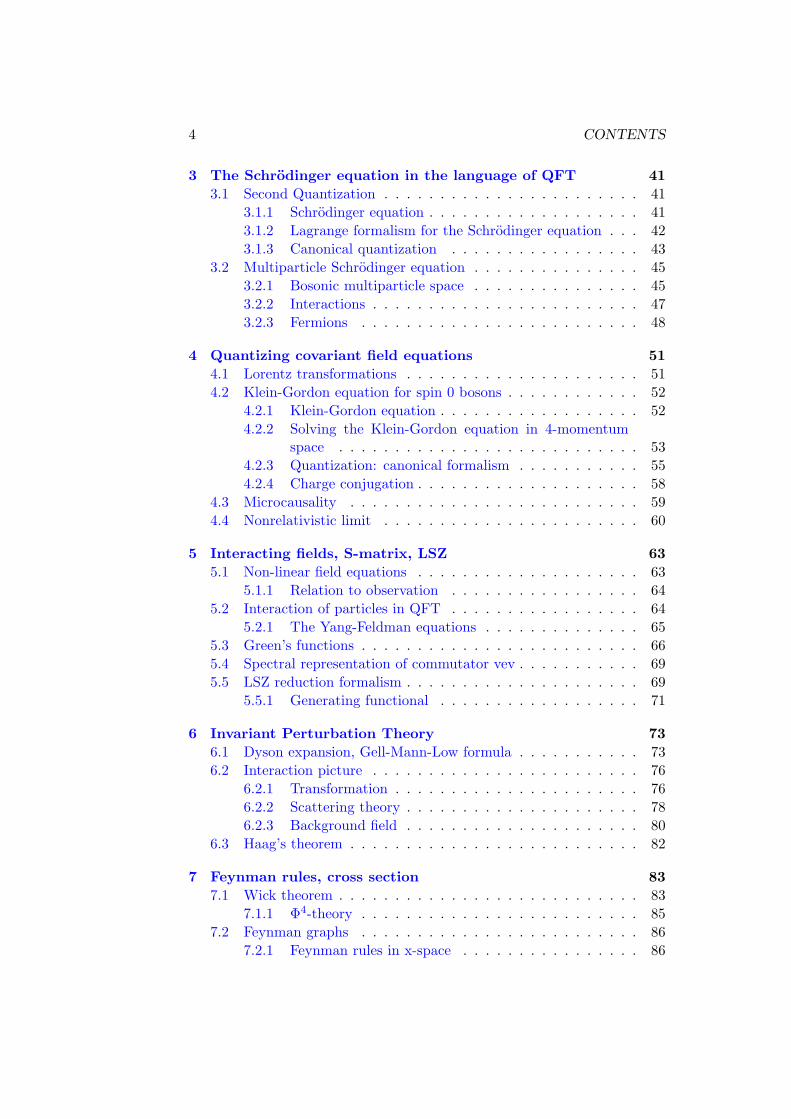
1.3. THE NEED FOR QFT 11
XS |xS〉 = ~xS |xS〉 (1.11)U†XSU︸ ︷︷ ︸
XH
U† |xS〉︸ ︷︷ ︸|x〉H
= ~xU† |xS〉︸ ︷︷ ︸|xH〉
Remark
In QM, multiparticle states can be represented, in spaces like
H1 ⊗ H2 ⊗ · · · ⊗ HN
which describe the whole space as a tensor product of the individualspaces of each of the N particles. This representation is used to describee.g. atomic structure, nuclear shells, or solid state physics, but the particlenumber N is always fixed!
1.3 The need for QFT
QFT is the quantum theory of fields, the main difference to QM being thehuge number of degrees of freedom (→∞). The principles, however, are thesame as those of QM. There is a (multiparticle) Hilbert space, called Fockspace, and a probability interpretation, all as we know them from QM. Sodon’t worry!
The electromagnetic wave equation is the prototype of a relativistic fieldequation: (
~∇2 − 1c
∂2
∂t2
)A(~x, t) = 0 (1.12)
It can be solved by a wave ansatz, which leads to:(k2 − ω2
c2
)Ake
−i(ωt−~k~x) = 0 (1.13)
With ~p = ~~k and E = ~ω we get the dispersion relation for photons inthe particle language: (
k2 − ω2
c2
)→ p2 − E2
c2= 0 (1.14)
Note that the wave equation is not a kind of Schrodinger equation for theprobability amplitude of photons. In this case it would be an equation for theprobability amplitude of a single photon, which would lead to contradictions.Consider the physics:

12 CHAPTER 1. INTRODUCTION
• It is very easy to produce ”soft” or ”collinear” quanta“soft”: E ∼ p ∼ small
“collinear”:~p−→
~p1→~p2→
with ~p = ~p1 + ~p2 and ~p || ~p1 || ~p2
• We want to measure x with precision ∆x. Assume ∆x ≤ λDeBroglie =~/p. Multiplying with ∆p and using the uncertainity relation we ob-tain ∆x ∆p ≥ ~ → ∆p ≥ p. This means that new particles may beproduced, because E2 = p2c2 for massless (highly relativistic) parti-cles.
More formally: the wave equation contains second derivatives with re-spect to time, which means that a probability interpretation like the one forthe Schrodinger equation fails (
√m2c2 + p2 is nonlocal).
Remarks
• The same problems arise for massive relativistic particles (e.g. pionπ±,0, e): we want to measure x with precision ∆x ≤ ~
mc = λComptonAgain using ∆x ∆p ≥ ~, we now obtain
∆p ≥ mc
With the relativistic relation
E2 = p2c2 +m2c4 → 2E∆E = 2p∆pc2
we see that
∆E = v∆p & mcv
This allows particle production for v → c. Thus, a particle can not belocalized without allowing for the production of further particles.
• ψ(~x, t) assumes that one can measure ~x arbitrarily exactly, but we havejust seen that then the particle number is not conserved. QM emergesfor non-relativistic massive particles in the limit of neglegible particleproduction (i.e., it is a special case of QFT). However, also for veryslow massive particles there are quantum field theoretical corrections:an example is the uncertainity relation ∆E∆t ≥ ~, which leads totunneling and particle production. For small times ∆t a very highenergy ∆E is possible, i.e. at small time scales we cannot excludeparticle production.

1.3. THE NEED FOR QFT 13
Figure 1.1: Particle production
In short
Relativistic field equations require to be treated in the framework of QFT,where particles can be produced and annihilated. Their interpretation isdifferent from that of the Schrodinger equation. The electromagnetic fieldhas nothing to do with the localization probability of a single photon.
Still: The principles of QM remain true!
Other relativistic field equations are the Klein-Gordon equation and theDirac equation. The Dirac equation, which contains only first order timederivatives, allows for a one particle interpretation in the nonrelativisticlimit, although not without further ado, as will be seen later.
We will first discuss free particles, and later their interactions, almostexclusively in the context of perturbation theory. Particularly interesting aregauge theories (electrodynamics, chromodynamics, flavordynamics).
This might give the impression that QFT was made exclusively for fun-damental theories, for elementary particle physics. However, it is also veryimportant in statistical mechanics and solid state physics (see e.g. the roleof path integrals and their relation to the partition function); and of coursehistorically, the connection between QFT and relativity was very important!

14 CHAPTER 1. INTRODUCTION
1.4 History
1925/1926: Heisenberg and Schrodinger develop their QM formalisms,which are proven to be equivalent
1926: Bohm, Heisenberg and Jordan begin developing QFT1927: Dirac postulates his equation and explains spontaneous emission1928: Jordan and Wigner (anti-commutation relations, Pauli principle)1929/1930: Heisenberg and Pauli develop the canonical formalism1930: Dirac works on hole theory and antiparticles; the positron is
detected1948: Schwinger, Feynman and Tomonaga publish on the Lamb shift;
the anomalous magnetic moment e− is explained1949: Dyson’s work leads to a better understanding of the Feynman
graph rules1954: Yang and Mills publish their (at the time mostly unnoticed)
article on non-Abelian gauge theories1955: Lehmann, Szymanzik and Zimmermann (S-matrix in QFT)1957: Bogoliubov and Parasiuk (renormalisation)1966: Hepp and ...1969: ... Zimmermann work out renormalisation to all orders
1.5 Harmonic oscillator, coherent states
1.5.1 Classical mechanics
In classical mechanics, we know the Hamiltonian of the harmonic oscillator:
H =1
2mp2 +
mω2
2x2
with the equations of motion
x =∂H
∂p=
p
mp = −∂H
∂x= −mω2x
(see Hamilton equations, sec. 1.2.1). By a canonical transformation, weobtain the holomorphic representation:
a = (√mωx+ i
p√mω
)/√
2
a∗ = (√mωx+ i
p√mω
)/√
2 (1.15)
x, p → a, ia∗
In terms of these new variables, the Hamiltonian becomes:
H =ω
2(a∗a+ aa∗)

1.5. HARMONIC OSCILLATOR, COHERENT STATES 15
The equations of motion are:
i ˙a∗ = −∂H∂a
= −ωa∗ (1.16)
˙a =∂H
∂(ia∗)= −iωa
These are first order differential equations, allowing us to solve for a, a∗:
a(t) = e−iωt a(0) (1.17)a∗(t) = eiωt a∗(0)
1.5.2 Quantization
We use the quantization rule known from QM:
Poisson-Bracket → i
~× commutator
For example:
p, xP = 1⇒ i
~[P,X] = 1
f(x, p) =∂f
∂xx+
∂f
∂pp = H, fP ⇒ f(X,P) =
i
~[H, f ]
When we quantize the harmonic oscillator, we promote a and a∗ to operators:
a, a∗ ⇒ a, a†
which obey the usual commutation relation:
i
~
[ia†, a
]= 1
In QM we will often find ~ included in a. So we can set ~ = 1, or define anew a, to make the equations look nicer:
a :=a√~⇒
[a,a†
]= 1
→ H = ~ω(a†a + aa†
)︸ ︷︷ ︸
a†a+1
⇒ H = ~ω(a†a +
12
)
The occupation number operator N is defined as
N := a†a

16 CHAPTER 1. INTRODUCTION
and has eigenvalues
N |n〉 = n |n〉 n = 0, 1, ...
|0〉 is the ground state. In this setting a and a† are the annihilation andcreation operators, and have the following actions:
a |n〉 =√n |n− 1〉 (1.18)
a† |n〉 =√n+ 1 |n+ 1〉 (1.19)
1.5.3 Coherent states
The states |n〉 do not correspond to quasiclassical states. The closest ap-proximations to classical states are called coherent states, which, in theHeisenberg picture, which we will use most frequently, are defined as fol-lows:
|λ〉 = Neλ(t)a†(t) |0〉 (1.20)
Fromi~∂
∂ta† = −
[H,a†
]= −a†~ω
we obtain→ a†(t) = eiωta†(0)→ λ(t) = e−iωtλ(0)
which, if plugged into the definition of a coherent state, gives:
|λ〉 = N
∞∑n=0
λna+n
n!|0〉 = N
∞∑n=1
λn√n!|n〉
To determine the normalization N , we take the inner product of |λ〉 withitself:
〈λ|λ〉 = |N |2∞∑n=0
|λ|2n
n!= |N |2e|λ|2 != 1
⇒ N = e−|λ|2/2 (1.21)
If we now apply the annihilation operator a to such a coherent state, weobtain:
a |λ〉 = N
∞∑n=1
λn(0)√n√
n!|n− 1〉 = λ |λ〉 (1.22)
We can also use this as a definition of coherent states. From the above,it follows that the expectation values of a and a† are given by
〈λ|a|λ〉 = λ⟨λ|a†|λ
⟩= λ∗

1.5. HARMONIC OSCILLATOR, COHERENT STATES 17
and ⟨λ|a†a|λ
⟩= |λ|2
Analogously, we can calculate a† |λ〉, which gives
a† |λ〉 =ddλ|λ〉 (1.23)
i.e., a and ia† act on coherent states as λ and i ddλ .
For coherent states, the sum of the variances of X and P is minimal, i.e.|λ〉 comes closest to classical motion.
For the variance in the occupation number N , we have:
(∆N)2 =⟨λ|(N− 〈N〉)2|λ
⟩=
⟨λ|N2|λ
⟩− 〈λ|N|λ〉2⟨
λ|a†aa†a|λ⟩
= |λ|4 + |λ|2⟨λ|a†a|λ
⟩= |λ|2
⇒ (∆N)2 = |λ|2 = 〈N〉
⇒ ∆N〈N〉
=1√〈N〉
(1.24)
The relative variance goes to 0 for large N.
Remarks
• Introducing coherent states:
In the Heisenberg picture, we have
a |λ〉 = λ |λ〉
|λ〉H = e−|λ|2/2 eλ(t)︸︷︷︸
e−iωt
a†(t) |0〉
In the Schrodinger picture, this becomes:
|λ〉S = e−iHt/~ |λ〉H= Neλ(t)a†(0) |0〉
• Coherent states are not orthogonal:⟨λ|λ′
⟩= e|λ−λ
′|2/2ei=(λ∗λ′) (1.25)

18 CHAPTER 1. INTRODUCTION
• The completeness relation holds for coherent states:
∫dλdλ∗
2πi|λ〉 〈λ| = 1 (1.26)
We can obtain this relation by expanding an inner product 〈n|m〉 inthe λ-basis and integrating:∫
dλdλ∗
2πi〈n|λ〉 〈λ|m〉 =
∫dλdλ∗
2πiNN∗
λn√n!λ∗m√m!
= δnm = 〈n|m〉
where in the second step we have used
〈λ|m〉 = ψm(λ∗) = Nλ∗m√m!
• The following normalization is often used in the literature:
〈λ|λ〉 = e|λ|2
In this case, the completeness relation changes:
∫dλdλ∗
2πie−λ
∗λ |λ〉 〈λ| = 1
• The representation of an arbitrary operator A in the λ-basis is asfollows:
〈λ|Af〉 =1
2πi
∫ ⟨λ|A|λ′
⟩︸ ︷︷ ︸A(λ∗,λ′)
⟨λ′|f
⟩dλ′ dλ′∗
A(λ∗, λ′) = 〈λ|n〉 〈n|A|m〉⟨m|λ′
⟩= Amn
(λ∗)n√n!
λ′m√m!e−|λ|
2/2e−|λ′|2/2 (with summing convention)
with A = Knma†nam (“normal ordered”)
Knm(λ∗, λ′) := Knmλ∗nλ′
m
⇒ A(λ∗, λ′) = e−(|λ|2+|λ′|2)/2K(λ∗, λ′)
• Applying this to a and a†, we plug in Knm = 0 except for n = 1,m = 0 for a†, and n = 0, m = 1 for a, in which cases K = 1. Thisgives a†(λ∗, λ′) = e−(|λ|2+|λ′|2)/2λ∗ and a(λ∗, λ′) = e−(|λ|2+|λ′|2)/2λ′
1.5. HARMONIC OSCILLATOR, COHERENT STATES 19
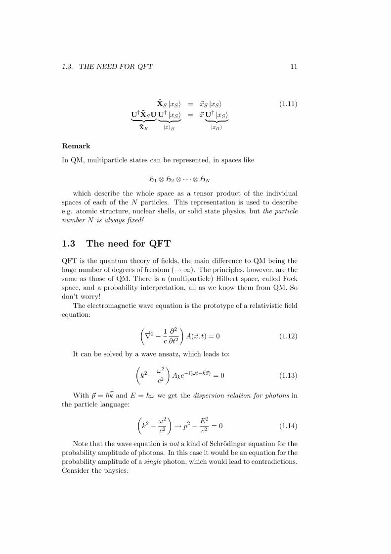
• Canonical transformations in phase space are symplectic (see e.g. F.Scheck, “Mechanik”). A general phase space vector
~zPh =(~x~p
)x1, . . . , xN = z1, . . . , zNp1, . . . , pN = zN+1, . . . , z2N
has the following Hamilton equation:
d~zPhdt
= J∂H
∂~zPh
with
J =(
0 1
−1 0
) (a “metric in phase space”, J−1 = −J
)A canonical transformation ~z → ~z′ preserves the Hamilton equation:
Mαβ :=∂zα∂z′β
α, β = 1, . . . 2N
M−1αβ :=
∂z′α∂zβ
z′α =∂z′α∂t
=∂z′α∂z′β
∂zβ∂t
=∂z′α∂zβ︸︷︷︸M−1
αβ
Jβγ∂H∂zγ
= M−1αβ Jβγ
∂H∂z′δ
∂z′δ∂zγ︸︷︷︸M−1
δγ
!= Jαδ∂H∂z′δ
(1.27)
⇒ M−1αβ JβγM
T−1γδ = Jαδ
⇒ J = MJMT (1.28)
M is a symplectic matrix (the M form a group)!
• The Poisson bracket
f, gPoisson (z) = − ∂f
∂zαJαβ
∂g
∂zβ
is invariant under canonical (symplectic) transformations.

20 CHAPTER 1. INTRODUCTION
1.6 The closed oscillator chain
1.6.1 The classical system
Figure 1.2: The closed oscillator chain
Let us consider a circular chain of radius R, with N masses m, connectedby springs with spring constant D. Let the ith mass be at a displacementqi = RΘi from some rest position, and let us impose the periodic boundarycondition q0 ≡ qN for convenience of writing. The distance between themasses when they are at rest is a = 2πR/N .
The Lagrangian for this system is:
L(q, q) =N∑j=1
[m
2q2j −
D
2(qj+1 − qj)2
]Varying ql, we get the equation of motion
mql +D (ql − ql−1 − (ql+1 − ql)) = 0
which is solved by the ansatz
ql(t) = ei(lk−ωt) (+vt)
leading to
mω2 + D︸︷︷︸mω2
(2− e−ik − e+ik
)︸ ︷︷ ︸
4 sin2 k2
= 0
Because of the periodic boundary condition qN = q0, we get Nk = 2πnwith n = 0, . . . , N − 1 or n = −N/2, . . . ,+N/2 − 1 (for even N), and weobtain for the oscillator modes

1.6. THE CLOSED OSCILLATOR CHAIN 21
ω2n =
4Dm︸︷︷︸4ω2
sin2 πn
N(1.29)
Superposition of modes gives the general solution for real qj(t):
qj(t) =1√N
N/2−1∑n=−N/2
[cne
i(2πnj/N−ωnt) + c∗ne−i(2πnj/N−ωnt)
](1.30)
(note that this is a Fourier expansion).The Hamiltonian is then given by:
H(q, p) =N∑j=1
[p2j
2m+D
2(qj − qj−1)
2
],
where pj = mqj , and the corresponding equations of motion are
pj = −∂H∂qj
, qj =∂H∂pj
.
To ensure that the the transformation (qj , pj) → (cn, c∗n) is canonical,we normalize cn and c∗n by defining the new canonical variables an and ia∗nthrough an =
√2mωncne−iωnt (cf. harmonic oscillator, sec. 1.5.1). These
variables are canonical:
an, ia∗mPoisson = −δnm, a, a = a∗, a∗ = 0
The new Hamiltonian is
H =∑n
12ωn(a∗nan + ana
∗n)
Note that this transformation is still classical. It is preferable, however,to discuss this in the already quantized version.
1.6.2 Quantization
The procedure is exactly the same as it was for the harmonic oscillator:
pl, ql → pl,ql
f(p, q), g(p, q)Poisson → i
~[f ,g]
an, a∗n → an, a†n
Then the an, ia†n fulfill the usual commutation relation

22 CHAPTER 1. INTRODUCTION
[an, a†m
]= i~δnm
and the Hamiltonian looks like this:
H =∑n
ωn
(a†nan +
12
~)
Exercise: obtain the commutator [pj , qj′ ] from [an, a†m] = i~δnm and
derive the Hamiltonian above (use∑N−1
n=0 e2πin(j−j′)/N = Nδjj′).
In the following we will often use units where ~ = 1. We will sometimesreinsert the factors of ~, in cases with experimental relevance; the same goesfor setting c = 1.
Defining a(†)n =
√~a(†)
n , the Hamiltonian becomes:
H =∑n
~ωn(a†nan +
12
)(1.31)
After quantization each mode n has an excitation number (the “occupa-tion number” of some quasiparticle-mode), as we have already seen in thecase of the harmonic oscillator. This begs the question whether, as a physi-cist, one can distiguish these modes (called phonons if they live in crystals)from “real” particles.
If one can see the “lattice” (e.g. a solid state crystal), the answer is yes,because a real particle should exist independently of the medium it livesin. One can not always see this medium, however, in particular when thecontinuum limit has been taken. Then, the “lattice” has become some sortof “ether”, which is not necessarily visible to the physicist, and might notbe needed anymore.
An interesting case is fundamental (super)string theory, where particlesare modes of strings.
The states on which the operators defined above act live in a Fock spaceF = H1 ⊗ H2 ⊗ · · · ⊗ HN , where Hi the Hilbert space of i-th mode. The“vacuum” state is denoted by |0〉, and has am |0〉 = 0 for all m.
General states
|n1, n2, . . . , nN 〉 =(a†1)
n1
√n1
(a†2)n2
√n2
. . .(a†N )nN
√nN
|0〉
are normalized eigenstates of H and have energy
E =∑m
~ωm(nm +
12
)Note: Elastic binding to lattice, mimicking a crystal, at xj = j2πR/N
gives a term −(m/2)Ω2q2j in L which shifts the ω2n in eq. (1.29) by +Ω2;
there is no zero mode.

1.6. THE CLOSED OSCILLATOR CHAIN 23
One can rewrite eq. (1.30) by substituting −n for n in the second term:
qj =N/2−1∑n=−N/2
e2πinj/N
[an + a†−n√
2mωn
]=
N/2−1∑n=−N/2
e2πinj/NQn
Similarly, one can introduce
Pn =√mωn
2i(an + a†−n)
Check the following relations:
[P−n,Ql] = −iδnl
and
H =∑n
12m
P−nPn +12mω2
nQ−nQn
with Pn = P†n and Qn = Q†n
1.6.3 Continuum limit
In the continuum limit, we take N to infinity and a to zero while keeping2πR = Na fixed. The index j becomes a continuous variable, leading to:
qj(t)→ q(x, t), x = a · j (1.32)
Note that in the “closed string” case discussed above, one does not haveelastic binding to the lattice like one has for a crystal, and x is defined upto an overall translation.
Now, we make the following translations:
(qj − qj−1)2 → a2
(∂q(x, t)∂x
)∑j
→ 1a
2πR∫0
dx
Further, we postulate
m = ρa with finite mass density ρ
D =σ
awith finite string density σ

24 CHAPTER 1. INTRODUCTION
and obtain the following Lagrangian:
Lcont =12
2πR∫0
dx
[ρ
(∂q(x, t)∂t
)2
− σ(∂q(x, t)∂x
)2]
(1.33)
The equations of motion
ρ∂2q(x, t)∂t2
− σ∂2q(x, t)∂x2
= 0
can be read off from the discontinous case. Later, we will obtain themdirectly from eq. (1.33).
Now, with c =√σ/ρ we can rewrite the above equation as:
∂2q
∂t2− c2 ∂
2q
∂x2= 0 (1.34)
Note: introducing elastic binding (cf. note in section 1.6.2) gives anadditional mass term −1
2
∫ 2πR0 dxρΩ2q2(x, t) in eq. (1.33), and −Ω2q in eq.
(1.34), which then has the form of a Klein-Gordon equation to be discussedin the next chapter.
Now, we can just translate our “discrete” solution to the continuum case,or we can make the following ansatz (from electrodynamics):
q(x, t) = Aei(kx−ωt)
Plugging this into eq. (1.34) gives
ω2 = c2k2
Imposing periodic boundary conditions q(0, t) = q(2πR, t) leads to
kn =n
R(n = 0,±1,±2, . . . )
which, in combination with ω2 = c2k2, gives
ωn =|n|cR
(1.35)
Note that in the finite N case, the continuum ωn is only approximatelyvalid. We have to use the formula from the discrete case:
ωn =
√4Dm
sin(π|n|N
)(1.36)
We expand this for small n, using the linear approximation for the sine:
ωn ∼√
4Dm
π|n|N
=2cπ|n|aN
=c|n|R

1.6. THE CLOSED OSCILLATOR CHAIN 25
(remember D = c2m/a2 and a = 2πR/N). This approximation is onlyallowed when π|n|
N < π4 ; then, we have:
ωn ≤c
R
N
4= ωc (1.37)
Note that in the above discussion, c does not always have to be the speedof light; it may also be a characteristic speed for the medium in which ourphonons are living.
1.6.4 Ground state energy
E0 =∑n
~ωn2
=+∞∑
n=−∞~|n|c2R
(1.38)
In the continuum limit the ground state energy is divergent! We will ob-serve such divergences more often in QFT; they are related to the continuumlimit and to interaction at a point, and require physical discussion.
In the finite N case:
E0 =~2
N/2−1∑n=−N/2
c
R
N
πsin(π|n|N
)
≈ ~2
1/2∫−1/2
dxc
R
N2
πsin(π|x|) (use x ∼ n
N)
E0
2πR≈ ~
2· 2 · 1
π· cN2
πR · 2πR
=~c2π3
N2
R2=
2~cπa2
withN2
R2=(
2πa
)2
Figure 1.3: Validity range for the linear approximation

26 CHAPTER 1. INTRODUCTION
The absolute value of E0 does not have a physical meaning (except ingeneral relativity, where it appears on the right hand side of the Einsteinequation), but we can compare ground state energy in two different physicalsituations; in doing so, we can observe the Casimir effect.
1.7 Summary
1.8 Literature
Literature list for QFT I and II; books marked with * are particularly rec-ommended for studies accompanying the lectures
1.8. LITERATURE 27
*L. H. Ryder Quantum Field Theory (Cambridge Univ. Press)rather elementary, clear, wide variety of subjects
*M. E. Peskin,D. E. Schroeder
An introduction to QFT (Addison-Wesley)
*M. Maggiore A modern Introduction to QFT (Oxford Univ. Press)*C. Itzykson,J. B. Zuber
Quantum Field Theory (Mc Graw Hill, also paper-back)comprehensive standard book, not always up to date,hard to read in a row (gauge theories)
*P. Ramond Field Theory, a modern Primer (Frontiers of Physics,Benjamin)early book on path integral formulation, non abeliangauge theory, unconventional
*S. Weinberg The Quantum Theory of Fields I, IIvery extensive, sometimes non-standard conventions
*K. Huang Quantum Field Theory: from operators to Path inte-grals (Wiley Interscience)looking to QFT outside elementary particle physicssee also Quarks... (World Scientific Publish.)
*M. Stone The Physics of Quantum Fields (Springer)Elementary, wide range
T. Kugo Eichtheorie (Springer)Thorough discussion of gauge theory quantization
E. Harris A Pedestrian Approach to QFT (Wiley, also in Ger-man)rather elementary, short
F. Mandl, G. Shaw Quantum Field Theory (Wiley Interscience)Elementary introduction
V. P. Nair Quantum Field Theory, A Modern Perspective(Springer)Interesting advanced chapters
A. Zee Quantum Field Theory in a Nutshell (Princeton Univ.Press)unconventional presentation of concepts, diverserange of topics
L. S. Brown Quantum Field Theory (Cambridge University Press)S. J. Chang Introduction to QFT (World Scientific, Lecture Notes
in Physics, Vol. 29)J. D. Bjorken, S. Drell *I. Rel. Quantenmechanik II. Rel. Quantentheorie
(BI 98 and 101) (II. outdated, no QCD)a standard book some decades ago
N. N. Bogoliubov,D. V. Shirkov
Quantum Fields (Benjamini, Cummings;..)
related to the famous monography of the same au-thors, which today is partly outdated
28 CHAPTER 1. INTRODUCTION
L. D. Fadeev,A. A. Starnov
Gauge Fields, Introduction to QFT (Benjamini,Cummings)advanced studies
R. J. Rivers Path Int. Methods in QFT (Cambdridge Mon. onMath. Phys.)
J. Zinn-Justin Quantum Field Theory and Critical Phenomena (Ox-ford Science Publications)the connection to statistical mechanics
I. J. R. Aitchison Relativistic Quantum Mechanics (Mac Millan)strong relation to elementary particle physics, ele-mentary
C. Nash Relativistic Quantum Fields (Academic Press)renormalization theory for φ4
R. P. Feynman Quantum Electrodynamic (Frontiers in physics, Ben-jamin. inl.)unconventional, somewhat outdated
J. M. Jauch,F. Rohrlich
The Theory of Photons and Electrons (Springer)
old QED-monographyA. L. Fetter,J. D. Walecka
Quantum theory of Many Particle Systems (McGrawHill)Feynman diagrams in solid-state physics
A. Smilga Lectures on Quantum Chromodynamics (World Sci-entific)
M. Le Bellac Quantum and Statistical Theory (Clarence Press, Ox-ford)Thermal QFT

Chapter 2
The free electromagneticfield; Klein-Gordon equation;quantization
We quantize the free electromagnetic field in the Coulomb/radiation gauge,analogously to the oscillator string. Then, we discuss electromagnetic emis-sion and absorption in this language. We introduce the Lagrange- andHamilton-formalisms for fields and present a more thorough discussion ofthe canonical quantization of the Klein-Gordon equation. To conclude, wecome back to the Maxwell equations in the canonical formalism.
2.1 The free electromagnetic field
2.1.1 Classical Maxwell theory
The classical source-free Maxwell equations are:
~∇ · ~B = 0, ~∇ · ~E = 0, ~∇× ~E = −1c
∂
∂t~B, ~∇× ~B =
1c
∂
∂t~E (2.1)
In the Coulomb/radiation gauge, we have
~∇ · ~A = 0, φ = 0, so ~E = −1c
∂
∂t~A
Using ~B = ~∇× ~A and Ampere’s law, we obtain
~∇×(~∇× ~A
)= ~∇
(~∇ · ~A
)︸ ︷︷ ︸
=0
−~∇ · ~∇ ~A = −1c
∂ ~A
∂t
29

30CHAPTER 2. FREE EM FIELD, KLEIN-GORDON EQ, QUANTIZATION
resulting in (∆− 1
c2∂2
∂t2
)~A(~x, t) = 0 (2.2)
for the wave equation.In order to solve the wave equation in a finite volume L3 with periodic
boundary conditions, we make the following ansatz, based on a Fouriertransform (later on called Fourier ansatz):
~A(~x, t) =1√L3
∑~k
N~k
(~a~k(t) e
i~k~x + ~a∗~k(t) e−i~k~x
)(2.3)
with normalization N~k and discrete kiL = 2πni.From ~∇· ~A = 0, we have ~k ·~a~k = 0, i.e. the solution has only transversal
modes; this is the origin of the name transversal gauge. The wave equationgives ~a~k ∝ eiωt, with dispersion relation c|~k| = ω. Now, let us calculate theenergy of the electromagnetic field:
E =18π
∫d3x
(~E2 + ~B2
)=
18π
∫d3x
(1c2
(∂
∂t~A
)2
+(~∇× ~A
)·(~∇× ~A
))
Through partial integration, the second term becomes
(−1)2(~A× ~∇
)·(~∇× ~A
)= ~A ·
(~∇×
(~∇× ~A
))↓ Coulomb gauge= − ~A ·∆ ~A
↓ partial integration= (~∇ ~A) · (~∇ ~A)︸ ︷︷ ︸
∂iAk∂iAk
leading to
E =18π
∫d3x
3∑i=1
(1c2
(∂
∂tAi
)2
+(~∇Ai
)2)
(2.4)
Substituting the Fourier ansatz gives
E =2L3
8πL3
1c2
∑~k
ω2~kN2(ω~k)
(~a~k ~a
∗~k
+ ~a∗~k ~a~k
)

2.1. THE FREE ELECTROMAGNETIC FIELD 31
Exercise: provide the intermediate steps. Now, using ω = c|~k| and orthogo-nality, we have ∫
V
d3x ei(~k−~k′)~x = L3δ~k,~k′
where a Kronecker delta appears because the k-indices are discrete (remem-ber that we had periodic boundary conditions).
The cross terms (~a~k ~a−~k+~a∗~k~a∗−~k
) in the sum come from both (∂ ~A/∂t)2/c2
and (~∇ ~A), but with opposite sign, so they cancel. Finally, choosing N =√2πc2/ωk, we obtain
E =12
∑~k
ω~k
(~a~k ~a
∗~k
+ ~a∗~k ~a~k
)with ~k · ~a~k = 0 (2.5)
which is a sum over harmonic oscillator terms.The Poynting vector is calculated similarly:
~P =1
4πc
∫d3x ~E × ~B =
∑~k
~k~a∗~k · ~a~k
which, with ~E × ~B = −1c
(∂∂t~A)×(~∇× ~A
), becomes:
~P = −1c
(~∇(∂
∂t~A
)· ~A−
(∂
∂t~A
)· ~∇ ~A
)The second term becomes zero after partial integration.
Note
• In the continuum limit, where L→∞, the sum is replaced by an inte-gral: Σ→
∫d3k/(2π)3L3. WithN ∝ 1√
L3, it followsA ∝
∫d3k/(2π)3(...),
and H = 1/2∫
d3k/(2π)3(...)
The expression (2.5) above can be interpreted intuitively as a collec-tion of an infinite number of harmonic oscillators, with ~a~k and i~a∗~k
asgeneralized coordinates and momenta (compare to the oscillator chainfrom chapter one). We will have to substantiate this heuristic inter-pretation when introducing the canonical formalism for fields in thenext section.
• The corresponding position (and momentum) operators cannot naıvelybe identified with the argument ~x of ~A(~x, t).

32CHAPTER 2. FREE EM FIELD, KLEIN-GORDON EQ, QUANTIZATION
Figure 2.1: Electromagnetic wave propagation
2.1.2 Quantization
The quantization is procedure is similar to the one for harmonic oscillator
i
~
[aσ~k , ia
†λ~k′
]= −δ~k,~k′δ
σ,λ, σ, λ = 1, 2 (2.6)
for transversal polarization degrees of freedom σ: ~a~k = ~e 1 a 1~k
+ ~e 2 a 2~k
with
~e 1 ⊥ ~e 2 ⊥ ~k.Promoting the ~a~k and i~a∗~k from eq. (2.5) to operators, we have
H =12
∑~k,σ
ω~k
(aσ~k a†σ~k + a†σ~k aσ~k
)leading to
H =∑~k,σ
ω~k
(a†σ~k aσ~k +
12
~)
(2.7)
Note that a†σ~k aσ~k = ~nσ~k is the occupation number of the harmonic oscil-
lator nσ~k and the zero-point energy of the ~k-mode is ~ω~k/2.Again, the space of states is the direct product space of the Hilbert-
spaces corresponding to the modes, called Fock-space:
H =∏~k,σ
⊗ H~k,σ ; states:∣∣∣nσ1~k, nσ2~k, . . . nσN
~k
⟩
E =∑~k,σ
~ω~k
(nσ~k +
12
); ~P =
∑~k,σ
~~k nσ~k
Here we have an infinite number of degrees of freedom (modes), eachwith its own occupation number as for the harmonic oscillator. Because

2.1. THE FREE ELECTROMAGNETIC FIELD 33
Figure 2.2: Absorption and Emission process
of the sum there is an infinite ground state energy, the so-called vacuumenergy. This can be removed it by normal ordering, : aa† : = a†a (movingall annihilation operators to the right of all creation operators), but this isad hoc. Infinite energy shifts are also a problem in general relativity, whereenergy density influences the curvature of spacetime.
2.1.3 Application: emission, absorption
Consider induced emission or absorption, or spontaneous emission due to aninteraction (in QM):
HI = − e
mc~p · ~A(~x, t). (2.8)
With a quantized electromagnetic field, we have
initial state |i〉 = |a〉Atom∣∣∣. . . nσ~k⟩
final state |f〉 = |b〉Atom∣∣∣. . . nσ~k ± 1
⟩With
~A(x, t) =1√L3
∑~k,σ
N(aσ~k ~e
σ~kei~k~x + a†σ~k
~eσ~k e−i~k~x
)we obtain
〈f |HI |i〉 = − e
mc
(2π~c2
L3ωk
)1/2 ⟨b|~p · ~eσ~k e
±i~k~x|a⟩
√nσ~k
+ 1√nσ~k
nσ~k= 0 means spontaneous emission (→ “natural line width”, considering
perturbation theory).Finally, we have
transition probability / time =2π~|〈f |HI |i〉|2 δ(Ef − Ei).

34CHAPTER 2. FREE EM FIELD, KLEIN-GORDON EQ, QUANTIZATION
2.1.4 Coherent states
To approximate an electromagnetic wave one introduces coherent states likefor the single harmonic oscillator, and expresses ~A, ~E, and ~B through ex-pectation values in these coherent states. First observe that with
E = −1c
∂
∂tA = −i
∑~k,σ
(2π~ωkL3
)1/2
~εσ~k
(aσ~k(t) e
i~k~x − a†σ~k (t) e−i~k~x)
〈n| E |n〉 = 0 for E between states with fixed photon number n. Also note[Nσ~k, E]6= 0 (2.9)
i.e. photon number and electric field can not be measured simultaneously.However, we also have⟨
n|E2
4π|n
⟩=
~ωL3
(n+
12
)6= 0.
Now consider a monochromatic coherent state∣∣∣λ,~k, σ⟩ = Neλ~k,σ(t)aσ
~k†|0〉~k,σ . (2.10)
and calculate⟨λ,~k, σ|E|λ,~k, σ
⟩= −i
(2π~ωL3
)1/2
~eσ~k
(λ~k,σ(t) e
i~k~x − λ∗~k,σ(t) e−i~k~x
)which is the Fourier-component of a monochromatic, polarized E. Observethat λ determines the amplitude. The conclusion is that for induced ab-sorption/emission, one can get back the normal QM description by usingcoherent states. (Note: the “Fock-space vacuum” |0〉 =
∏~k,σ⊗ |0〉~k,σ allows
for product states of (2.10) in the more general case.)
2.2 Klein-Gordon equation
2.2.1 Lagrange formalism for field equations
Consider an action
S[L] =∫ t1
t0
dt∫
d3x L(
Φ(~x, t),(∂
∂tΦ), ~∇Φ
)︸ ︷︷ ︸
L(Φ(·,t),... )
and a field Φ(~x, t). Discretizing the field, using a lattice, turns it into avector, with position serving as an index: Φ(~xi, t) → Φi(t). Note, however,

2.2. KLEIN-GORDON EQUATION 35
Figure 2.3: Field Lattice
that we retain infinitely many degrees of freedom even in the discretizedcase.
The Lagrangian L is a functional of Φ(·, t), the action S of Φ(·, ·). Wepostulate δS[L] = 0 with a variational derivative, i.e. S is extremal (chang-ing Φ at position ~x and time t).
Functional derivatives
For a functional F (Φ(·)), we have
F (Φ(·) + εξ(·))− F (Φ(·)) = ε
∫dx
δF
δΦ(x)ξ(x) +O(ε2)
which defines the functional derivative δFδΦ(x) . An elegant, if a little heuristic,
choice for the perturbation function ξ is ξ(x) = δ(x− x).
limε→0
F (Φ(x) + εδ(x− x))− F (Φ(x))ε
=δF
δΦ(x)
∣∣∣∣x=x
Remarks:
• Discretization (x→ xi,Φ(xi)→ Φi) turns the derivative into a gradi-ent and δ(x− x) into δij .
• If the functional is defined as F (Φ(·)) =∫
dx F (Φ(x)), then
δF (Φ(·))δΦ(x)
=∂F (Φ(x))∂Φ(x)
i.e. we also can get along without functional derivative notation.
• Φ(xa) is a functional itself:
Φ(·)→ Φ(xa)

36CHAPTER 2. FREE EM FIELD, KLEIN-GORDON EQ, QUANTIZATION
δΦ(xa)δΦ(x)
∣∣∣∣x=x
= limε→0
Φ(xa) + εδ(xa − x)− Φ(xa)ε
= δ(xa − x)
This will be important later on when calculating the Poisson bracketof Φ,Π.
Applying the above to the action, we get:
δS =∫ t1
t0
dt∫
d3x′∂L∂Φ
ε(t)δ(~x′ − ~x) +∂L
∂ (∂Φ/∂t)∂ε(t)∂t
δ(~x′ − ~x)
+∂L∂Φ|i
ε(t)∂
∂x′iδ(~x′ − ~x)
=
part.int.∫ t1
t0
dt ε(t)∫
d3x′δ(~x′ − ~x)∂L∂Φ− d
dt∂L
∂ (∂Φ/∂t)− ∂
∂x′i
∂L∂Φ|i
where Φ|i := ∂Φ
∂xi. There are no boundary terms in this formulation with
δ-functions and ε(t0) = ε(t1) = 0. In the original, and more “orthodox”,formulation, without delta’s, Φ → Φ + εξ(~x, t), and for all ξ, ξ = 0 at theendpoints t0 and t1 and |~x| → ∞.
Regardless of the formulation, one has
δS = 0 ∀ ε(t), ~x.
resulting in∂L∂Φ− ∂
∂t
∂L∂ (∂Φ/∂t)
− ∂
∂xi
∂L∂Φ|i
= 0 (2.11)
for the field equation.Remark: in case of a finite volume, one takes periodic boundary condi-
tions in x-space.
The momentum field is defined as
Π(~x, t) =∂L
∂(∂Φ/∂t)=
∂L∂(∂Φ/∂t)
Note: the (canonical) momentum field Π(~x, t) is not the momentum P ofthe field.
From the Lagrangian density L and associated momentum field Π weobtain the Hamiltonian by means of a Legendre transform.
H =∫
d3x
Π(~x, t)
∂
∂tΦ(~x, t)− L(Φ,
∂
∂tΦ, ~∇Φ)
︸ ︷︷ ︸
Hamiltonian density H

2.2. KLEIN-GORDON EQUATION 37
The Hamilton equations read
∂Φ∂t
=δHδΠ
=∂H∂Π
∂Π∂t
= −δHδΦ
= −(∂H∂Φ− ∂|i
∂H∂Φ|i
)(2.12)
The Poisson bracket is defined analogously to the discrete case:
A(Π,Φ), B(Π,Φ)Poisson :=∫ (
δA
δΠ(~x)δB
δΦ(~x)− δB
δΠ(~x)δA
δΦ(~x)
)d3x = δ(~x−~x′)
Exercise: show that this indeed gives a delta function. Note that Φ,Π(~x)are particular functionals, see remark page before.
2.2.2 Wave equation, Klein-Gordon equation
The wave equation (1c2∂2
∂t2−∆
)︸ ︷︷ ︸
=
A(~x, t) = 0
is solved by the Fourier ansatz
A = e±i(ωt−~k~x) with − ω2
c2+ k2 = 0 .
With E = ~ω and p = ~k, this translates into the photon energy relation:
−E2
c2+ p2 = 0
Similarly, for massive particles we have
−E2
c2+ p2 +m2c2 = 0
or, dividing by ~
−ω2(~k)c2
+ k2 +m2c2
~2= 0
This translates to the differential equation(1c2∂2
∂t2−∆ +
m2c2
~
)Φ(~x, t) = 0 (2.13)
which is the promised Klein-Gordon equation for a scalar field. The equationfollows from the Lagrangian
L =12
[1c2
(∂Φ∂t
)2
−(~∇Φ)2− m2c2
~2Φ2
].
38CHAPTER 2. FREE EM FIELD, KLEIN-GORDON EQ, QUANTIZATION
The corresponding momentum field is
Π(~x, t) =∂L
∂(∂∂tΦ) =
(∂
∂tΦ)
resulting in the following Hamiltonian density:
H =12
[1c2
(∂
∂tΦ)2
+(~∇Φ)2
+m2c2
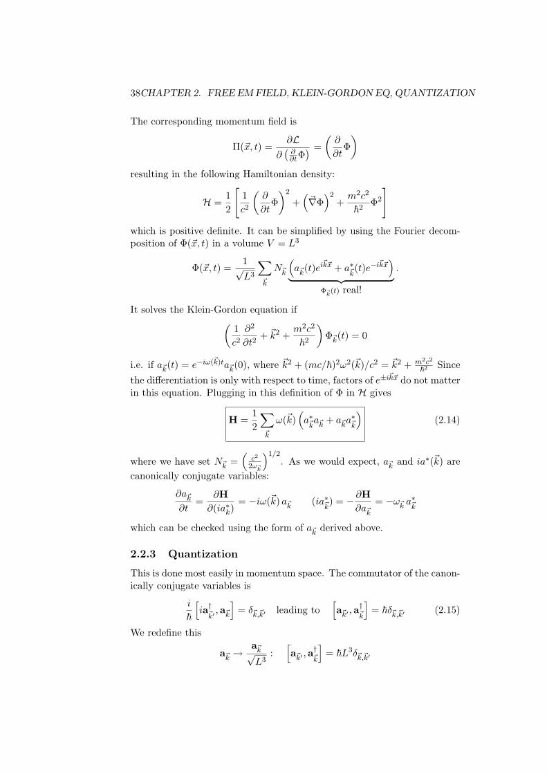
~2Φ2
]which is positive definite. It can be simplified by using the Fourier decom-position of Φ(~x, t) in a volume V = L3
Φ(~x, t) =1√L3
∑~k
N~k
(a~k(t)e
i~k~x + a∗~k(t)e−i~k~x
)︸ ︷︷ ︸
Φ~k(t) real!
.
It solves the Klein-Gordon equation if(1c2∂2
∂t2+ ~k2 +
m2c2
~2
)Φ~k(t) = 0
i.e. if a~k(t) = e−iω(~k)ta~k(0), where ~k2 + (mc/~)2ω2(~k)/c2 = ~k2 + m2c2
~2 Since
the differentiation is only with respect to time, factors of e±i~k~x do not matterin this equation. Plugging in this definition of Φ in H gives
H =12
∑~k
ω(~k)(a∗~ka~k + a~ka
∗~k
)(2.14)
where we have set N~k =(c2
2ω~k
)1/2. As we would expect, a~k and ia∗(~k) are
canonically conjugate variables:
∂a~k∂t
=∂H∂(ia∗k)
= −iω(~k) a~k (ia∗~k) = −∂H∂a~k
= −ω~k a∗~k
which can be checked using the form of a~k derived above.
2.2.3 Quantization
This is done most easily in momentum space. The commutator of the canon-ically conjugate variables is
i
~
[ia†~k′ ,a~k
]= δ~k,~k′ leading to
[a~k′ ,a
†~k
]= ~δ~k,~k′ (2.15)
We redefine this
a~k →a~k√L3
:[a~k′ ,a
†~k
]= ~L3δ~k,~k′

2.2. KLEIN-GORDON EQUATION 39
(again, see the oscillator chain). Since we have for L→∞∑~k∼~n
δ~k,~k′ = 1 ⇒∫
d3k
(2π)3L3 δ3(~k − ~k′)(2π)3
L3= 1
we see that in the continuous case, the commutator must be
[a~k′ ,a†~k] = ~(2π)3δ3(~k − ~k′) (2.16)
We could have derived this directly from the canonical formalism, pro-moting the Poisson bracket to a commutator:
Φ(~x, t),Π(~x′, t)Poisson
= −δ3(~x− ~x′)~/i ⇓ quantization[
Φ(~x, t),Π(~x′, t)]
= i~δ3(~x− ~x′)
from which the above result for a~k follows. Exercise: invert the relationbetween Φ,Π and a, ia† and calculate
[a,a†
]. Alternatively, which is easier,
plug in Φ,Π in terms of a, a† and obtain the relation above.Of course we have now
Φ(~x, t) =∫
d3k
(2π)31√
2ω(~k)
(a~k(t) e
i~k~x + a†~k(t) e−i~k~x
)(2.17)
H =∫
d3k
(2π)312ω(~k)
(a†~k(t)a~k(t) + a~k(t)a
†~k(t))
(2.18)
Remarks
Since we know the wave equation from electromagnetics, and since we used arelativistic dispersion relation between ω and ~k to begin with, it is clear thatour equation is relativistically invariant, as well as the Lagrangian relatedto it. We will learn more about this later on. The remarkable aspect ofthis whole episode is that canonical quantization, where time plays a specialrole, can be brought into consistency with relativity, where time and spaceare on the same footing.
L =12∂µΦ ∂µΦ− m2
2Φ2 . . .
2.2.4 The Maxwell equations in Lagrange formalism
Here, we will shortly discuss gauge theories (again, more details will follow).For now, we will restrict ourselves to the free case, i.e. without sources. Wewill use units where x0 = t, c = 1. Consider the electromagnetic tensor:
Fµν = ∂νAµ − ∂µAν (2.19)
40CHAPTER 2. FREE EM FIELD, KLEIN-GORDON EQ, QUANTIZATION
and note that it contains ~E and ~B in relativistic notation.The electric and magnetic fields appear in it as follows:
F 0i = Ei; F ik = εiklBl
A0 = φ; ~E = −~∇φ− ∂
∂t~A; ~B = ~∇× ~A
with ~∇ = ∂∂xi = ∂i = −∂i. So, two Maxwell equations are automatically
fulfilled. What remains to be shown is
~∇ · ~E = 0 and ~∇× ~B =∂ ~E
∂t
or, in other symbols,∂Fµν
∂xν= 0
With eq. (2.5), this becomes
∂2Aµ − ∂ν∂µAν = 0 (2.20)
In the Coulomb gauge, ∂iAi = 0 and φ = A0 = 0 (hence the term radiationgauge). Hence, eq. (2.20) reduces to ∂2Aµ = 0, which is just the waveequation, as ∂2 = ∂/∂x02 − ~∇2. The equation for Aµ follows from L =−1/4FµνFµν if one varies the Aµ and Aν independently (Exercise: work thisout.)
Note: in terms of ~E and ~B, L = 1/2( ~E2− ~B2), but we do not vary withrespect to these variables.
Calculating the canonical momenta (see Bjorken and Drell, vol. II) gives:
Π0 =∂L
∂(∂A0/∂t)= 0; Πk =
∂L∂(∂Ak/∂t)
= −∂Ak
∂t− ∂A0
∂xk= Ek
Inspecting the canonical formalism, we get the following result, which looksreasonable:
H = Πk ∂
∂tAk − L =
12( ~E2 + ~B2) + ~E · ~∇φ
H =∫
d3x H =12
∫d3x ( ~E2 + ~B2)
The last term can be disposed of through partial integration, since ~∇ ~E = 0.This is not without problems, however, since ~∇ ~E = 0 is violated by boththe fact that Π0 = 0, and the canonical commutator of Ak and Πk, which isgiven by [
Πi(~x, t), Ak(~x′, t)]
?= −iδ(~x− ~x′) δik
Indeed it turns out that in this case, we have to quantize with constraints ina more rigorous approach (see the literature on the Dirac bracket, which is

2.2. KLEIN-GORDON EQUATION 41
a special line of research). Note that working with constraints already popsup in classical field equations.
The simplest implementation of this idea is to do like is done in QED:take the Coulomb gauge.
L =∫
d3x L =∫ (−1
2∂Aµ∂xν
∂Aµ
∂xν+
12∂Aν∂xµ
∂Aµ
∂xν
)d3x
↓ Last term: partial integration, use ∂iAi = 0, A0 = 0→= 0
=12
∫∂ν ~A ∂ν ~A d3x.
We get 3 times the scalar case. Varying this separately for the two transver-sal and one longitudinal ( ~Along) components of ~A with the constraint that~∇ · ~A = 0, leads us to the canonical picture for ~Etrans(~∇ · ~E = 0) and for~Atrans(~∇ · ~A = 0), as was used in heuristic expose.

42CHAPTER 2. FREE EM FIELD, KLEIN-GORDON EQ, QUANTIZATION

Chapter 3
The Schrodinger equation inthe language of QFT
3.1 Second Quantization
For radiative transitions, the electromagnetic field is described by an oper-ator in Fock space, whereas the atom retains its ‘old’ QM description, i.e.with an ei~k~X, where the position is the operator ~X.
Now, the following question comes up: can we treat the Schrodingerequation, written down according to the rules of the correspondence prin-ciple, in its x-space form, like an ordinary field equation and quantize it?This sounds odd, since it is already quantized; why do it again? The pointis that we want QM to be a special case of QFT, as mentioned in chapter1, and therefore, it should be possible to express it in the language of QFT.This is called second quantization.
Note that we are not looking for new physics: QM has been testedthoroughly, and looks far too nice to throw away.
3.1.1 Schrodinger equation
In classical mechanics, we have E = ~p2/2m+V (~x); following the correspon-dence principle, this gives
i~∂
∂tψ(~(x), t) =
[(−~2~∇2
2m
)+ V (~x)
]︸ ︷︷ ︸
HSchr
ψ(~x, t) (3.1)
This has stationary solutions ψn = φn(~x)e−iEnt/~; we will also useEn/~ = ωn. General solutions, obtained from a generalized Fourier trans-form, are
ψ(~x, t) =∑n
an(t)φn(~x) (3.2)
43

44CHAPTER 3. THE SCHRODINGER EQUATION IN THE LANGUAGE OF QFT
where an(t) ∝ e−iωnt and the φn form a complete set of orthonormalfunctions.
In the QFT quantization, the functions an(t) are promoted to operatorsan(t); as usual, we are in the Heisenberg picture. The final result of thissecond quantization will be:
H =∫d3xψ†op(~x, t)HSchrψop(~x, t) (3.3)
which is an operator in Fock space. In terms of an, we have
H =∑n
Ena†nan (3.4)
where the an and ia†n are canonically conjugate operators in the Hamiltonianformalism. Let us now consider in detail how we get this result.
3.1.2 Lagrange formalism for the Schrodinger equation
In order to quantize the Schrodinger equation, we will treat it as an ordinaryfield equation, for which we will first develop the Lagrange formalism. TheLagrangian density is:
L = i~ψ∗ψ − ~2~∇ψ∗ · ~∇ψ2m
− V (~x)ψ∗ψ (3.5)
Following the usual procedure, we obtain the momentum fields:
Πψ =∂L∂ψ
= i~ψ∗; Πψ∗ = 0 (3.6)
We could obtain our field equation by varying L with respect to the realand imaginary parts of ψ, but we can also vary with respect to ψ∗ and ψ,since these are complex conjugates. This gives:
i~ψ +~∇ · ~∇ψ
2m− V (~x)ψ = 0 (3.7)
which is the Schrodinger equation, as we had hoped. Now, our Hamiltoniandensity (as used in eq. (3.3)) is given by
H = i~ψ∗ψ − L = ~2~∇ψ∗ · ~∇ψ
2m+ V (~x)ψ∗ψ (3.8)
Here, ψ and i~ψ∗ are canonical conjugates. In this equation, we could alsointroduce electromagnetic coupling.
Note that we could also have taken a more symmetric Lagrangian density,i~2 (ψ∗ψ − ψ∗ψ) to obtain this result.

3.1. SECOND QUANTIZATION 45
3.1.3 Canonical quantization
The canonical quantization relation, where the ψ and ψ∗ are promoted toψop and ψ†op, is given by
[ψop(~x, t), i~ψ†op(~x′, t)] = i~δ3(~x− ~x′) (3.9)
Note that the factor i~ appears on both sides of the equation, and hencecancels. In terms of the a(†)
n , we have∑n,n′
[an,a†n′ ]φn(~x)φn′(~x
′) = δ3(~x− ~x′) (3.10)
where the generation and annihilation operators fulfill their usual commu-tation rule
[an,a†n′ ] = δn,n′ (3.11)
This gives the completeness relation: the φn(~x) form a complete basis.The Hamiltonian operator H =
∫d3xH is, as discussed in chapter 1,
given byH =
∑n
Ena†nan (3.12)
Using eq. (3.11), we find the Heisenberg equations for the an and a†n:
d
dtan(t) =
i
~[H,an] = −iωnan(t) (3.13)
d
dta†n(t) =
−i~
[H,a†n] = iωna†n(t) (3.14)
For the ψop and ψ†op, we have:
i~d
dtψop(~x, t) = − [H, ψop(~x, t)] (3.15)
i~d
dtψ†op(~x, t) = [H, ψ†op(~x, t)] (3.16)
The energy states in Fock space are obtained as usually, by applying a†n tothe vacuum. The action of an and a†n on a state is given by
an |. . . , Nn, . . . 〉 =√Nn |. . . , Nn − 1, . . . 〉
a†n |. . . , Nn, . . . 〉 =√Nn + 1 |. . . , Nn + 1, . . . 〉
Letting the ψ(†)op (~x, t) act on the vacuum gives:
ψop(~x, t) |0〉 = 0, (3.17)
46CHAPTER 3. THE SCHRODINGER EQUATION IN THE LANGUAGE OF QFT
since ψop contains only annihilators, and
ψ†op(~x, t) |0〉 = ~|X〉H (3.18)
which is a state with sharp position. The position ~X is fixed, but describedby time-varying Hilbert space vectors, which is where the time dependencecomes into the picture.
Exercise: prove eq. (3.18). Hint: use the Schrodinger equation forψ(~x, t) = 〈X|ψH〉, or write ~XH(t) =
∫d3x′ψ†op(~x′, t)~x′ψop(~x, t) and show
that ~XH~|X〉H = ~X |X〉H .
For the particle number density, we have:
n(~x, t) = ψ†op(~x, t)ψop(~x, t) (3.19)
n(~x′, t)ψ†op(~x′, t) |0〉 = δ(~x− ~x′)ψ†op(~x, t) |0〉︸ ︷︷ ︸
localized
(3.20)
The total particle number N should be conserved, since we are dealing withnormal QM systems, where particle production is forbidden. Indeed, usingeq. (3.19) and the Heisenberg equation, we find that∫
d3xn(~x, t) = N
is conserved.
Quite generally, for any Schrodinger operator AS(XS ,PS), we have anassociated (Heisenberg) operator AF (ock) acting on the Fock space of theone-particle state:
AF (t) =∫d3xψ†op(~x, t)ASψop(~x, t) (3.21)
Using the commutator [ψop, ψ†op] = δ3, the fact that double annihilation on a
one-particle state gives zero (ψopψop |1 part.〉 = 0), and the definition above,we see that commutation relations of the form
[AS ,BS ] = CS
translate to
[AF ,BF ] = CF
(the notation AH is also used for AF ).An example of the above correspondence is the momentum operator,
which generates translations. It is defined by U~a = e−i~PF ·~a/~, where now
~PF acts on states in the Fock space. Applying it to a state |~x〉 gives

3.2. MULTIPARTICLE SCHRODINGER EQUATION 47
U~a ψ†op(~x, t) |0〉︸ ︷︷ ︸
=|~x〉
= U~aψ†op(~x, t)U
†~aU~a |0〉︸ ︷︷ ︸
=|0〉
Using the fact that |0〉 is invariant under translations, this becomes:
|~x+ ~a〉 = ψ†op(~x+ ~a, t) |0〉
For infinitesimal translations, we have[~PF , ψ
(†)op
]=
~i~∇ψ(†)
op
For rotations, generated by the angular momentum operator ~JF , we havethe same procedure: U~ω = e−i
~JF ·~ω/~, where ~JF is given by
~JF =∫d3xψ†op(~x, t)
(~XS ×
~i~∇)ψop(~x, t)
And again, for infinitesimal rotations:[~JF , ψ(†)
op
]=(~XS ×
~i~∇)ψ(†)op
3.2 Multiparticle Schrodinger equation
3.2.1 Bosonic multiparticle space
The description of systems consisting of more than one identical particlesis a nice application of the new QFT-inspired formalism obtained from thesecond quantization. Note again that we are still talking about QM as weknow it; only the language has changed.
Consider a system of N identical particles, which can be in states like∣∣∣n~k1n~k2 . . . n~kl
⟩=∣∣∣n~k1⟩⊗ ∣∣∣n~k2⟩⊗ · · · ⊗ ∣∣∣n~kl
⟩where the possibility of polarization has been left out to avoid drowning
in indices. The states∣∣n~k⟩ are given by
∣∣n~k⟩ =(a†~k)
n~k√n~k!|0〉 (3.22)
General states (still without polarization) look like this:
∞∑l=1
∑~k1...~kl
f(n~k1~k1, . . . , n~kl
~kl)∣∣∣n~k1 . . . n~kl
⟩(3.23)

48CHAPTER 3. THE SCHRODINGER EQUATION IN THE LANGUAGE OF QFT
Here, the order of the ~ki is arbitrary, since the a†~kicommute. The total
particle number is given by N =∑l
i=1 n~ki. These states live in a Fock space
obtained by a direct product of harmonic oscillator Hilbert spaces:
F =∏l=1
⊗Hosc~kl
They obviously inherit the linear structure of their constituents. Simi-larly, the inner product between two such states is obtained by taking theinner product in each H~k separately.
Another way of obtaining F is summing spaces with fixed particle num-bers:
F = H(0) ⊕ H(1) ⊕ · · · ⊕ H(l) =∑N
⊕H(n)
where
H(i) =∏i
⊗H(1) symmetrized
is the Hilbert space for i identical particles.
|~xi . . . ~xl〉H = Nsψ†op(~x1, t) . . . ψ†op(~xl, t) |0〉 (3.24)
The ψ†op generate identical particles, and hence commute. They are definedas follows:
ψ†op(~xj , t) =
∑~k
N~ka†~k(t)e−i~k·~x for free particles∑
~k
a†n(t)φ∗n(~xj) j = 1, . . . , l for bound particles(3.25)
Because of the fact that the ψ†op commute, we obtain l! terms with the sameset of ~ki in the free particles-case. This gives rise to a factor of l! in theinner product of a state with itself. This factor is always the same (exercise:show this), even if some of the ~k are identical. Examples are the case whereall ~k are different and the case of m identical ~k: in the first case, the normsquared of the state gets a factor l!, as just mentioned, and in the second,it is a factor (
lm
)·m!(l −m)! = l!
So, we set the normalization coefficient in eq. (3.24) Ns = 1/√l!.
Exercise: show, using the normalization coefficient derived above, thatthe following identity holds for a function fsym that is symmetric in the xl:∫
d3x′1 . . . d3x′l⟨~x1 . . . ~xl|~x′1 . . . ~x′l
⟩fsym(~x′1 . . . ~x
′l) = fsym(~x1 . . . ~xl)

3.2. MULTIPARTICLE SCHRODINGER EQUATION 49
3.2.2 Interactions
The total Hamiltonian can be split up into the parts concerning the individ-ual particles, parts resulting from interactions between two particles, etc.:
H = H(1) +H(2) + . . . (3.26)
The parts H(i) are defined as follows:
H(1) =∫d3xψ†op(~x, t)
(−~∇2
2m+ V (~x
)ψop(~x, t) (3.27)
H(2) =∫d3xd3x′ψ†op(~x, t)ψ
†op(~x′, t)V (~x, ~x′)ψop(~x, t)ψop(~x′, t)(3.28)
The interaction potential V (~x, ~x′) = V ∗(~x, ~x′) is self-adjoint, e.g. e2/|~x−~x′|for the interaction between two electrons.
Exercise: using [ψop(~x, t), ψ†op(~x′, t)] = δ3(~x− ~x′), show that
i~∂
∂tψ(~x1, . . . , ~xl, t)︸ ︷︷ ︸=H〈~x1...~xl|ψ〉H
= i~∂
∂t〈0| ψop(~x1, t) . . . ψop(~xl, 1)√
l!|ψ〉H
= 〈0| − [H(1) +H(2),ψop(~x1, t) . . . ψop(~xl, t)√
l!|ψ〉
!= 〈0|l∑
i=1
H(1)S (~xi,
~i~∇i) +
12
l∑i,j=1,i6=j
V (~xi, ~xj)
×ψop(~x1, t) . . . ψop(~x1, t)√
l!|ψ〉
= (H(1)S +H
(2)S )ψ(~x1, . . . , ~xl, t)
Given that we are dealing with two-body interactions here, instead of thesingle particles discussed so far, one could think that the commutation rela-tion between ψop and ψ†op might not be the same as before. However, sincethe canonical momentum remains unchanged, we know that the old relationmust still hold.
We started with the linear Schrodinger equation, but we could also havestarted with a nonlinear equation, such as the Gross-Pitaevsky equationfor Bose-gasses. In this case, we would have to give up the superpositionprinciple for probability amplitudes. Since we are doing nonrelativistic QMhere, we prefer taking into account nonlinear parts only in H(2) and higherorders. Of course, one can also apply ordinary perturbative QFT, as will bediscussed later on.

50CHAPTER 3. THE SCHRODINGER EQUATION IN THE LANGUAGE OF QFT
Remark
With the results obtained above, we can write any interaction completely inquantized fields. The electromagnetic interaction, with ~A(x), is, as we willsee later on, obtained by minimal gauge coupling:
~i~∇ → ~
i~∇− e
c~A
H0 =∫d3xψ†op(~x, t)
1
2m
(~i~∇)2
+ V (~x)
ψop(~x, t) +
18π
∫d3x( ~E2 + ~B2)
HI = H(2) +∫d3xψ†op(~x, t)
[− e~imc
~A · ~∇+e2
2mc2~A2
]ψop(~x, t)
where ψ, ψ† and ~A are now quantum fields.
3.2.3 Fermions
We know from QM that we need the Pauli exclusion principle for electrons,protons, and other particles with half-integer spin. Later on, this will appearas a necessary consequence of QFT; we will see this in our discussion of theDirac equation. Here, only the results will be given: fermionic fields arequantized by substituting anti-commutators, rather than commutators, forthe Poisson bracket. We postulate:
[cn, c†n′ ]+ = cnc
†n′ + c†n′cn = δnn′ (3.29)
[cn, cn′ ]+ = [c†n, c†n′ ]+ = 0 (3.30)
(the notation ·, · is often used as an alternative for [·, ·]+.)Let us investigate the consequences of postulating anticommutating cre-
ation and annihilation operators. A striking result is that is immediatelyobvious is that c2
n = c†2n = 0. Now, consider the action of the occupationnumber operator N = c†c, N |n〉 = n |n〉. Let it act on a state c |n〉:
Nc |n〉 = c† cc︸︷︷︸=0
|n〉 = 0 =
= (−cc† + 1)c |n〉 = (−cN + c) |n〉 = (−n+ 1)c |n〉 = 0
So, either n = 1 or c |n〉 = 0. Now, let it act on a state c†:
Nc† |n〉 = c†cc† |n〉 = c†(−c†︸ ︷︷ ︸=0
c + 1) |n〉 = c† |n〉 = (−n+ 1)c† |n〉
3.2. MULTIPARTICLE SCHRODINGER EQUATION 51
So, either n = 0 or c† |n〉 = 0, giving the following relations:
c† |1〉 = 0, c |0〉 = 0 (3.31)c† |0〉 = |1〉 , c |1〉 = |0〉 (3.32)
In other words, the only occupation numbers are 0 and 1, as we wanted forfermions. The normalization is as follows:
〈0|0〉 = 1 (3.33)〈1|1〉 = 〈0| c†c |0〉 = 〈0| − cc† + 1 |0〉 = 〈0|0〉 = 1 (3.34)
A general fermion state is:
∑~k1...~kl
l∏i=1
f(~k1 . . .~kl)c†~ki|0〉 (3.35)
with n~ki= 1. Since the c†~ki
anticommute,∏
c†~kiis totally antisymmetric,
which means that only the totally antisymmetric part of f is interesting.In x-space, states look like this:
|~x1(t) . . . ~xl(t)〉 =1√l!ψ†op(~x1, t) . . . ψ†op(~x1, t) |0〉 (3.36)
where the ψ†op are, as usual, general solutions of the field equations:
ψ†op(~x, t) =∑n
c†nφ∗n(~x) (3.37)
A state with l different oscillators occupied is given by:
1√l!
∑1,...,lP
(−1)Pφ∗kp1(~x1) . . . φ∗kpl
(~xl)c†k1. . . c†kl
|0〉 =
1√l!
∣∣∣∣∣∣∣∣∣φ∗k1(~x1) . . . φ∗kl
(~x1)φ∗k1(~x2) . . . φ∗kl
(~x2)...
...φ∗k1(~xl) . . . φ∗kl
(~xl)
∣∣∣∣∣∣∣∣∣× c†k1 . . . c†kl|0〉 (3.38)
The determinant is called Slater-determinant, and gives rise to antisymmet-ric wave functions. It arises from the permutations which are summed overwith changing sign (the part
∑1,...,lP (−1)P in the left hand side).

52CHAPTER 3. THE SCHRODINGER EQUATION IN THE LANGUAGE OF QFT
Chapter 4
Quantizing covariant fieldequations
So far, our discussion of linear field equations has been quite generic, withthe exception of the electromagnetic wave equation. The importance of thisspecial case is indicated by the fact that it led Einstein to special relativity,and was the first triumph of QFT, which was absolutely essential for theacceptance of the theory. Therefore, it seems to make sense for us to in-spect the relativistic aspects of the QFT quantization. Later on, a thoroughclassification of Lorentz covariant fields will be given; here we start with thesimplest case, the Klein-Gordon equation. (Note that the wave equation isa special case of the Klein-Gordon equation: the one where m = 0.)
4.1 Lorentz transformations
We define contravariant and covariant spacetime vectors
xµ = (x0, ~x) contravariant (4.1)xµ = gµνx
ν covariant (4.2)
with the metric tensor (in Cartesian coordinates)
gµν =
1−1
−1−1
(4.3)
and x0 = ct. Hereafter, we will use units where c = 1, so x0 = t. Now, weset
x2 = xµxµ = (x0)2 − ~x2 = xµgµνxν
53

54 CHAPTER 4. QUANTIZING COVARIANT FIELD EQUATIONS
This is invariant under Lorentz transformations:
x′µ = Λµνxν (4.4)
for which the shorthand x′ = Λx is frequently used. This invariance meansthat
x2 = x′2 (4.5)
which requires
xµgµνxν = Λµνx
νgµνΛνµxµ ⇒
gνµ = ΛT µν gµνΛνµ (4.6)
where we have relabelled µ → ν and ν → µ on the left hand side. Inshorthand, we write
g = ΛT gΛ (4.7)
The gradient, ∂/∂xµ, is a covariant vector if xµ is a contravariant vector:
∂
∂x′µ=∂xν
∂x′µ∂
∂xν= (Λ−1)νµ
∂
∂xν= (Λ−1)T ν
µ
∂
∂xν
where we have used that x′ = Λx, x = Λ−1x′, and hence ∂xν/∂x′µ =(Λ−1)νµ. So ∂/∂xµ = ∂µ transforms with (Λ−1)T , i.e. like a covariant vector:
x′µ = gµνx′ν = gµνΛνλx
λ
= gµνΛνλ gλσ︸︷︷︸
=gλσ
xσ
which, using gΛg = (ΛT )−1 = (Λ−1)T , gives
x′µ = (Λ−1)T σµ xσ
4.2 Klein-Gordon equation for spin 0 bosons
4.2.1 Klein-Gordon equation
Let us begin by studying the simplest case of the Lorentz group: a scalarfield, denoted by Φ(x). It can be transformed by a Lorentz transformationor a translation, giving the following general transformation:
Φ(x)→ Φ′(x) = Φ(Λ−1(x− a))
This is the active view of symmetry transformations. Above, we have usedthat
Φ′(x′) = Φ(x) with x′ = Λx+ a (4.8)

4.2. KLEIN-GORDON EQUATION FOR SPIN 0 BOSONS 55
Figure 4.1: Transformation of Φ(x)
We already know the Klein-Gordon equation:
(∂µ∂µ +m2)Φ(x) = 0 (4.9)
(here written in units where ~ = c = 1). In components, it looks like this:[(∂
∂x0
)2
−(∂
∂xi
)2
+m2
]Φ(x0, ~x) = 0
(note that due to the squaring of the second term, the Einstein summingconvention applies to the index i). It is form invariant under Lorentz trans-formations, since both m2 and ∂µ∂µ transform like scalars, which are invari-ant under Lorentz transformations:
(∂′µ∂′µ +m2)Φ′(x′) = 0 → (rename x→ x′)
(∂µ∂µ +m2)Φ′(x) = 0
Hence Φ′(x) is a solution of eq. (4.9) if Φ(x) is one.
4.2.2 Solving the Klein-Gordon equation in 4-momentumspace
The general solution is obtained from a Fourier transform:
Φ(x) =∫
d4k
(2π)4Φ(k)e−ikµxµ
(4.10)
Plugging this into eq. (4.9) gives
(−k2 +m2)Φ(k) = 0
so

56 CHAPTER 4. QUANTIZING COVARIANT FIELD EQUATIONS
Φ(k) = a(k)2πδ(k2 −m2)θ(k0) + a(k)2πδ(k2 −m2)θ(−k0)
which we insert into eq. (4.10) after substituting k → −k in the second term(a(−k)→ b∗(k)):
Φ(x) =∫
d4k
(2π)3δ(k2 −m2)θ(k0)
a(k)e−ikx + b∗(k)eikx
(4.11)
Here, b∗(k)eikx represents the negative energy solutions.For real fields, this means b∗(k) = a∗(k), i.e. a(−k) = a∗(k); see chapter
2. We can rewrite a complex field Φ(x) in terms of two real fields Φ1 andΦ2:
Φ = (Φ1 + iΦ2)/√
2Φ∗ = (Φ1 − iΦ2)/
√2
yielding for a(k) and b(k):
a(k) = (a1(k) + ia2(k))/√
2 (4.12)b(k) = (a1(k)− ia2(k))/
√2 (4.13)
Lorentz invariants
δ(k2 −m2) is Lorentz invariant: it makes sure the solution lies on the massshell. θ(k0) is Lorentz invariant on this mass shell (exercise: show this),and
∫d4k is Lorentz invariant as well, since k′ = Λk, and |det Λ| = 1, so∫
d4k =∫d4k′. This implies that∫
d4k
(2π)3δ(k2 −m2)θ(k0) =
∫d3k
(2π)3
∫dk0δ(k2
0 − ~k2 −m2)θ(k0)
=∫
d3k
(2π)31
2k0,+where k0,+ = +
√k0
is Lorentz invariant, and, finally, that Φ(x) itself is a Lorentz scalar. To seethis, rewrite eq. (4.11) as
Φ(x) =∫
d3k
(2π)31
2k0,+
a(k)e−ikx + b∗(k)eikx
and observe that the part between braces consists only of scalars. Later on,we will sometimes write a(~k) instead of a(k), since k lies on the mass shell,and hence has only the degrees of freedom of the three-momentum.
The normalization of the a(k) obtained above is somewhat different fromthe one used in chapter 2, since it has been adapted to the relativistic char-acter of the equation. The a’s are not exactly the ones from the harmonicoscillator case.
4.2. KLEIN-GORDON EQUATION FOR SPIN 0 BOSONS 57
Reversing the equation, we can obtain Φ out of it:
a(~k) = i
∫d3xeikx
←→∂0 Φ(x)
:= i
∫d3x
(−∂e
ikx
∂x0Φ(x) + eikx
∂Φ(x)∂x0
)b∗(~k) = −i
∫d3xe−ikx
←→∂0 Φ(x)
Note that the inner product
(Φ1,Φ2) = i
∫Φ∗1(x)
←→∂0 Φ2(x)d3x
is only positive definite for positive energy solutions, as the differentiationwith respect to x0 brings down a factor of k0,+.
Exercise: show that θ(k0) is Lorentz invariant. We also have k′0 =Λ 0a k0 + Λ i
0 ki. If k lies on the mass shell and k0 > 0, we have the followinginequalities:
|~k| < k0∑i(Λ i
0 )2 < (Λ 00 )2
writing ΛT gΛ = g in orthogonal coordinates (i.e. using the Minkowskimetric). If Λ 0
0 > 1, we are dealing with the orthochronous Lorentz group,which we will encounter later on.
4.2.3 Quantization: canonical formalism
The Lagrange density corresponding to a real field Φ(x) with eq. (4.9) as‘equation of motion’ is:
L =12(∂µΦ(x)∂µΦ(x)−m2Φ2(x)
)(4.14)
For a complex field Φ = (Φ1 + iΦ2)/√
2, we have
Lcom =12
2∑j=1
∂µΦj(x)∂µΦj(x)−m2Φ2
j (x)
= ∂µΦ∗(x)∂µΦ(x)−m2Φ∗(x)Φ(x)
Note that here, we use x = (x0, ~x) and ∂µΦ∂µΦ = ∂∂x0 Φ ∂
∂x0 Φ− ∂∂xi Φ ∂
∂xi Φ.Now, in the real case, we vary the Lagrangians with respect to Φ. In the
complex case, we can choose between Φ1,2 and Φ, Φ∗, of which the latter
58 CHAPTER 4. QUANTIZING COVARIANT FIELD EQUATIONS
is the more practical one. This gives us the Euler-Lagrange equations ofmotion:
− ∂
∂xµ
(∂L
∂( ∂Φ∂xµ )
)+∂L∂Φ
= 0 (4.15)
Note that the derivative ∂∂xµ transforms like a covariant vector, whereas
∂L∂( ∂Φ
∂xµ )is contravariant. This makes the first term a scalar, as it should be,
since the second one is a scalar as well.In the complex case, we obtain eq. (4.15) with Φ∗ instead of Φ from
varying with respect to Φ, and with Φ from varying with respect to Φ∗.To obtain the Hamiltonian density, we need the momentum fields:
ΠΦ(x) =∂L
∂( ∂Φ∂x0 )
=∂Φ∂x0
(4.16)
This gives the Hamiltonian density
H(x) = ΠΦ∂Φ∂x0− L =
12
[(∂Φ∂x0
)2
+(∂Φ∂xi
)2
+m2Φ2
](4.17)
In the complex case, we have
ΠΦ(x) =∂Φ∗
∂x0
ΠΦ∗(x) =∂Φ∂x0
and
Hcom(x) = ΠΦ∂Φ∂x0
+ ΠΦ∗∂Φ∗
∂x0− L = ΠΦΠΦ∗ +
∂Φ∗
∂xi∂Φ∂xi
+m2Φ∗Φ (4.18)
Both the complex and the real Hamiltonian densities are positive definite.From these, we obtain the Hamiltonian
H =∫d3xH(Π,Φ) (4.19)
Later on, we will see that this is the zero component of a four-vector.The Poisson bracket of these fields is the usual delta function:
Π(~x, t),Φ(~x′, t)
P= δ3(~x− ~x′) (4.20)
Quantizing this according to the usual rule gives the commutator[Π(~x, t),Φ(~x′, t)
]= −iδ3(~x− ~x′) (4.21)

4.2. KLEIN-GORDON EQUATION FOR SPIN 0 BOSONS 59
where ~ = 1. This does not look Lorentz covariant, since time and spaceare treated differently here. Later on, however, we will see that it is Lorentzcovariant. In the complex case, we have the same commutator as above, orits Hermitian conjugate:[
ΠΦ†(~x, t),Φ†(~x′, t)]
= −iδ3(~x− ~x′) (4.22)
This implies:
[∂Φ†(~x, t)
∂t,Φ(~x′, t)
]= −iδ3(~x− ~x′) =
[∂Φ(~x, t)
∂t,Φ†(~x′, t)
]Rewriting the field Φ(x) as a Fourier transform, we get
Φ(x) =∫
d3k
(2π)31
2k0,+
a(~k)e−ikx + a†(~k)eikx
(4.23)
or, for the complex case,
Φcom(x) =∫
d3k
(2π)31
2k0,+
a(~k)e−ikx + b†(~k)eikx
(4.24)
Inserting this in the definition of H gives the following Hamiltonian for thereal field:
H =∫d3xH =
∫d3k
(2π)314
a†(~k)a(~k) + a(~k)a†(~k)
(4.25)
Exercise: provide the intermediate steps. In the complex case, we have
Hcom =∫
d3k
(2π)314
a†(~k)a(~k) + a(~k)a†(~k)
+∫
d3k
(2π)314
b†(~k)b(~k) + b(~k)b†(~k)
(4.26)
which features a second type of oscillators, the “b-particles”.Note that this integration measure is really the Lorentz covariant dk, fol-
lowed by a factor of k0,+/2, which we know from the traditional Hamiltonian(it was called ω/2 before):
H =∫
d3k
(2π)31
2k0,+
k0,+
2(. . . ) =
∫d3k
(2π)314
(. . . )
When quantizing this field, we promoted the a and a∗ to operators a anda†, and similarly for the b in the complex case. The a, a† have the followingcommutation relation:
[a(~k),a†(~k′)] = 2k0,+(2π)3δ3(~k − ~k′) (4.27)

60 CHAPTER 4. QUANTIZING COVARIANT FIELD EQUATIONS
The same holds for the b’s. Also, any a commutes with any b, i.e. they arecompletely independent and on the same level.
Note: in the literature, the factor of 2k0,+ is sometimes omitted; thenotation employed here, which does include it, along with some π-factors,is called the “Cambridge notation”.
Both the a, a† and the b, b† build up a symmetric Fock space. Mixed a,b combinations therefore act in a product space. A state with n a-particlesand n′ b-particles looks like this:
n+n′∏i=1
d3ki(2π)32ki,0
c(k1 . . . kn)√n!
˜c(kn+1 . . . kn′)√n′!
×
a†(~k1) . . .a†(~kn)b†(~kn+1) . . .b†(~kn+n′) |0〉 (4.28)
Since these states have to be normalized, the normalization functions c and˜c have to obey:
〈ψ|ψ〉 = 1 =∫
d3k1
(2π)32k1,0. . .
d3kn+n′
(2π)32kn+n′,0|c|2|˜c|2 = 1 (4.29)
4.2.4 Charge conjugation
Consider the Hermitian conjugate of a complex quantized field Φ(x):
Φ†(x) =∫
a†(~k)eikx + b(~k)e−ikx
The roles of a and b have clearly been exchanged. Hence, we can concludethat the b-particles are antiparticles of the a-particles. This is illustratedmore clearly by the coupling of a complex (“π-meson”) field Φ(x) to anelectromagnetic field:
∂µ → ∂µ + ieAµ = DµCoupling a charged field to a vector potential, one replaces the momen-
tum pµ ↔ i∂µ by the kinetic momentum in the Hamiltonian pµ−eAµ; this iscalled “minimal coupling” and leads to the modified Klein-Gordon equation:
(DµDµ +m2)Φ(x) = 0 (4.30)
which is gauge invariant under the following transformations:
Φ→ Φ′(x) = e−ieΛ(x)Φ(x)Aµ(x)→ A′µ(x) = Aµ + ∂µΛ
since the “covariant derivative” transforms as
D′µΦ′(x) = (∂µ + ieAµ + ie∂µΛ)e−ieΛ(x)Φ(x)
= e−ieΛ(x)DµΦ(x) (4.31)

4.3. MICROCAUSALITY 61
(∂µ acting on e−ieΛ(x) gives a term −ie∂µΛ in the factor between brackets).Φ∗ fulfills the same equation with e→ −e , which is the same as replac-
ing Dµ with D∗µ. Since changing Φ into Φ∗ means exchanging a and b, thisexchange really achieves charge conjugation. Now, we would like to havea charge conjugation operator, in order to make this operation mathemati-cally more fitting to the model. This operator should be unitary: reversinga charge conjugation should give the original situation. Its action should ofcourse be:
Φ†(x) = UCΦ(x)U−1C (U−1
C = U†C) (4.32)
(this is equivalent to b(~k) = UCa(~k)U†C). Exercise: show that this operatoris given by
UC = exp(−iπ
∫dk
12
a†a + b†b− a†b− b†a
)Hint: use
Φ2 =Φ− Φ∗
i√
2=∫dk
(a− bi√
2ei~k·~x − a† − b†
i√
2e−i
~k·~x)
Then, rewrite the integrand in the formula for UC as a†2(~k)a2(~k), wherea2 := a−b
i√
2.
4.3 Microcausality
In its quantized form, the Klein-Gordon equation still should fulfill the re-quirements of special relativity. In evaluating whether it does, we will usecomplex fields; we could also have used real ones.
The commutator of a field Φ(x) at position x with its Hermitian conju-gate at position y is given by
[Φ(x),Φ†(y)] =: i∆(x− y)
=∫
d3k
2k0(2π)3d3k′
2k0(2π)3([a(~k),a†(~k′)]e−ikx+ik
′y + [b(~k),b†(~k′)]eikx−ik′y)
=∫
d3k
2k0(2π)3(e−ik(x−y) − eik(x−y)
)(4.33)
Renaming ~k → −~k in the second term, the integrand can be rewritten as−2iei~k·(~x−~y) sin(k0(x0 − y0)). This implies that if x0 = y0, ∆ = 0. Now, ifthe difference between x and y is spacelike, one can always transform to aframe of reference where (x − y)0 = 0. Since the commutator is invariantunder transformations, this means that for a spacelike pair of points, ∆ isalways zero. Thus, microcausality is conserved. Commutators of Φ or Φ†
alone vanish identically.

62 CHAPTER 4. QUANTIZING COVARIANT FIELD EQUATIONS
4.4 Nonrelativistic limit
We have the Klein-Gordon equation:
(∂20 − ~∂2 +m2)Φ(~x, t) = 0 (4.34)
Extracting the time derivative and expanding around m gives:
i∂0Φ(~x, t) = ±(m2 − ~∂2)1/2Φ(~x, t)
= ±(m− 1
2m~∂2 + . . .
)Φ(~x, t)
Retaining only the first two terms, and choosing the positive sign convention,we obtain the non-relativistic Schrodinger equation with a constant potential(resulting from the first term, m). Note that this is only valid in the non-relativistic limit, where |~k| << m: the full operator (m2− ~∂2)1/2 is nonlocal.
The inner product of a field with itself is given by:
(Φ,Φ) =∫d3xΦ∗(x)
←→∂ 0Φ(x) =
∫d3k
(2π)32k0
(a(~k)a∗(~k)− b∗(~k)b(~k)
)(4.35)
which is not positive definite. We can interpret |a(~k)|2 d3k(2π)32k0
as a proba-bility density if we consider only solutions with positive energy, i.e. whereb ≡ 0. Negative energy solutions would have disastrous results in interactiontheory.
In QM, the normalization factor of 1/(2π)32k0,+ is absent, and we justhave |Ψ(~k)|2d3k. Fourier transforming this gives the wave function Ψ(~x, t),which has a positive definite inner product for positive energy solutions.
Taking a localised Ψ~x0(~x, 0) = δ3(~x− ~x0), Fourier transforming back to
momentum space (⇒ a(~k)) we obtain Φ~x0(~x, 0), Φ~x0
(~x, 0) ∼(mr
)5/4H5/4(imr)
with r = |~x − ~x0|. Although this drops exponentially for r >> m−1, it isnot really localized.
Figure 4.2: Unsharp position
4.4. NONRELATIVISTIC LIMIT 63
The position operator
In position space, the position operator ~X becomes ~x0:
~XΦ~x0(~x, 0) = ~x0Φ~x0
(~x, 0)
In momentum space, we get something different from QM:
~X→ i~∇~p −i~p
2p20
The extra term of −i~p/2p20 is responsible for the zitterbewegung, which ob-
scures the exact position.

64 CHAPTER 4. QUANTIZING COVARIANT FIELD EQUATIONS

Chapter 5
Interacting fields, S-matrix,LSZ reduction
5.1 Non-linear field equations
Last chapter, we studied the Klein-Gordon equation, (∂2 + m2)Φ(x) = 0.Now, let us consider non-linear equations, such as:
(∂2 +m2)Φ(x) =λ
3!Φ3 (5.1)
where we have a (local) self interaction of the field, which is obtained from aterm Lint in L: −λ4! Φ4. Sometimes it is convenient to separate the nonlineareffects, introducing a source field j(x) in the above equation::
(∂2 +m2)Φ(x) = j(x) (5.2)
and obtain solutions to eq. (5.1) in this way.In eq. (5.1), the canonical momentum field is unchanged, since Lint
does not contain any derivatives, and therefore the canonical commutationrelations are still valid. However, the Fourier decomposition used before isnot available here, because the equation is, as said, non-linear.
Remark
It is possible to construct the Noether currents and charges (the generatorsof transformations) and check whether Lorentz covariance is consistent withthe canonical commutation relations. This turns out to be the case, as wewill see later on.
In this course, we will mostly treat Lint as a small perturbation of thefree theory, which brings us to perturbation theory. First, however, wewill present a more general framework: the LSZ formalism, named after itsinventors Lehmann, Szymanzik and Zimmermann.
65
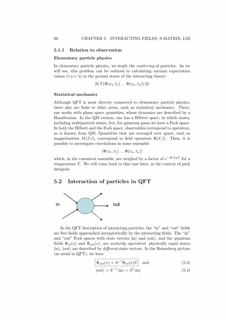
66 CHAPTER 5. INTERACTING FIELDS, S-MATRIX, LSZ
5.1.1 Relation to observation
Elementary particle physics
In elementary particle physics, we study the scattering of particles. As wewill see, this problem can be reduced to calculating vacuum expectationvalues (v.e.v.’s) in the ground states of the interacting theory:
〈0|T (Φ(x1, t1) . . .Φ(xn, tn)) |0〉
Statistical mechanics
Although QFT is most directly connected to elementary particle physics,there also are links to other areas, such as statistical mechanics. There,one works with phase space quantities, whose dynamics are described by aHamiltonian. In the QM version, one has a Hilbert space, in which states,including multiparticle states, live; for quantum gases we have a Fock space.In both the Hilbert and the Fock space, observables correspond to operators,as is known from QM. Quantities that are averaged over space, such asmagnetisation M(~x, t), correspond to field operators Φ(~x, t). Then, it ispossible to investigate correlations in some ensemble
〈Φ(x1, t1) . . .Φ(xn, tn)〉
which, in the canonical ensemble, are weighed by a factor of e−H/kBT for atemperature T . We will come back to this case later, in the context of pathintegrals.
5.2 Interaction of particles in QFT
In the QFT description of interacting particles, the “in” and “out” fieldsare free fields approached asymptotically by the interacting fields. The “in”and “out” Fock spaces with state vectors |in〉 and |out〉, and the quantumfields Φin(x) and Φout(x), are unitarily equivalent: physically equal states|in〉, |out〉 are described by different state vectors. In the Heisenberg picture(as usual in QFT), we have
Φout(x) = S−1Φin(x)S and (5.3)
|out〉 = S−1 |in〉 = S† |in〉 (5.4)
5.2. INTERACTION OF PARTICLES IN QFT 67
with a unitary matrix S. Note that states containing less than two particlesdo not interact, as there is nothing to interact with:
|0〉in = |0〉out and |1〉in = |1〉outNow consider the limit where Φ(x) approaches Φin(x). The equation
(∂2 +m2)Φ(x) = j(x)
is solved by
Φ(x) = Φhom(x) +∫d4y Gret(x− y,m)j(y) (5.5)
where Gret is the retarded Green’s function, for which we have
(∂2 +m2)Gret(x− y,m) = δ4(x− y)and Gret(x− y,m) = 0 for x0 < y0
since the current j(x) influences only the future. From this equation, onemight naıvely assume that Φ(x) approaches the homogeneous solution asx0 → −∞, as mentioned at the beginning of this section. However, beforebeing able to assume this, one has to consider the covergence type. Theproblem is that the normalizations of Φ(x) and Φhom(x) are not generallythe same:
〈1~p|Φin(x) |0〉 6= 〈1~p|Φ(x) |0〉Φin(x) = eiPxΦin(0)e−iPx
Φ(x) = eiPxΦ(0)e−iPx
Both matrix elements are proportional to eiPx, but the norms are not equal,since Φ(x) |0〉 is in general not a pure one-particle state. States in Hilbert orFock space are normalized by their inner product with themselves, whereasoperators are normalized through commutators. So, what we have to con-sider is the convergence of Φ(x) towards Φin(x) multiplied by some scalar:
limx0→−∞
Φ(x) = Z1/2Φin(x)︸ ︷︷ ︸hom. solution
(5.6)
5.2.1 The Yang-Feldman equations
This idea has been implemented in the Yang-Feldman equations:
√ZΦin(x) = Φ(x)−
∫d4xGret(x− y,m)j(y) (5.7)
√ZΦout(x) = Φ(x)−
∫d4xGav(x− y,m)j(y) (5.8)
68 CHAPTER 5. INTERACTING FIELDS, S-MATRIX, LSZ
These can be used as definitions for Φin,out(x), since√Z is fixed by the
canonical commutation relation for Φin,out. It also is the same in both equa-tions. To see this, consider 〈1-part.|Φ(x) |0〉, and note that in this case, thesecond term does not contribute.
We do not have convergence in the operator sense (or strong convergence)for Φ(x): it is not true that Φ(x)→ Z1/2Φin(x), since this is not compatiblewith the canonical commutation relations. Assuming Φ(x) → Z1/2Φin(x),the equal time commutator would give:
[∂0Φ(x),Φ(y)]x0=y0 = −iδ3(~x− ~y) so
Z[∂0Φin(x),Φ(y)]x0=y0 = −iδ3(~x− ~y) for x0 → −∞
which cannot be true, since Z is not in general equal to 1. Therefore, weonly have convergence in the following sense:
• Only individual matrix elements converge. Since not all matrix ele-ments necessarily converge at the same rate, the whole matrix, or theoperator, does not converge.
• Wave packets built out of matrix elements, such as
Φ(f, t) = i
∫d3xf∗(x)
←→∂ 0Φ(~x, t)
with (∂2 +m2)f = 0, also converge.
This type of convergence is also called weak convergence.
Remark
j(~x, t)→ 0 for t→ ±∞ in the operator sense is not possible, unless one goesto the Bogoliubov-Shirkov construction, where couplings are made to go tozero as t→∞ (see their textbook on QFT).
5.3 Green’s functions
We have already seen the causal Green’s function,
DC(x′ − x) = i∆(x′ − x) = [Φfree(x′),Φfree(x)]= 〈0| [Φfree(x′),Φfree(x)] |0〉
which is given by
DC(x′ − x) =∫
d3k
2k0(2π)3(e−ik(x
′−x) − eik(x′−x))
(5.9)

5.3. GREEN’S FUNCTIONS 69
and is zero for (x′ − x)2 < 0, i.e. for spacelike displacements. Exercise:show that DC can be written as follows with the help of the zeroth-orderBessel function J0:
DC(x) = DC(x0, ~r) =i
4πr∂
∂r
J0(m((x0)2 − r2)1/2) (x0)2 > r2
0 (x0)2 < r2
The canonical commutation relation ([∂tΦ(x′),Φ(x′)]ET = −iδ3(~x′− ~x))gives
∂
∂x′0DC(x′ − x) = −iδ3(~x′ − ~x) (5.10)
Now, we can see that the retarded and advanced Green’s functions fromelectrodynamics are given by:
DR(x′ − x) = θ(x′0 − x0)DC(x′ − x) (5.11)
DA(x′ − x) = θ(x0 − x′0)DC(x′ − x) (5.12)
Exercise: check that (∂2x′ +m
2)DR,A(x′−x) = −iδ4(x′−x). Use ∂∂x′0
θ(x′0−x0) = δ(x′0 − x0) and the fact that δ′ is defined by partial integration.
The usual way to obtain DR,A is solving the differential equation via aFourier transform and realizing the boundary conditions by a choice at thepoles of the integrand:
Figure 5.1: Integration path for DR
DR(x) =∫
d4p
(2π)4i
p2 −m2e−ipx
= −∫
d3p
(2π)3
∫dp0
2πi1
p20 − ~p2 −m2
e−ip0x0ei~p·~x (5.13)
For x0 > 0, we close the integration loop in the lower half plane, and forx0 < 0 in the upper half plane. For DA, we pass by the poles in the lowerhalf plane and close the loop in the upper half plane. The denominator inthe integrand comes from the two poles:
1p0 + (~p2 +m2)1/2 + iε
× 1p0 − (~p2 +m2)1/2 + iε
∼ 1p20 − ~p2 −m2 + iε

70 CHAPTER 5. INTERACTING FIELDS, S-MATRIX, LSZ
Figure 5.2: Integration path for DA
Later on, the Feynman propagator will be important; it is obtained bythe following integration path, and is given by
DF (x) =∫
d4p
(2π)4i
p2 −m2 + iεe−ipx (5.14)
Figure 5.3: Integration path for DF
For x0 > 0, the integral loop is closed in the lower half plane, so thispole contributes ∫
d3p
(2π)31
2p0,+e−ipx
∣∣∣∣p0=p0,+
which is the first half of the commutator from DC ; for x0 < 0, the loop isclosed in the upper half plane, which gives the second half:
−∫
d3p
(2π)31
2p0,+e−ipx
∣∣∣∣p0=−p0,+
Altogether, this gives
DF (x− x′) = θ(x′0 − x0) 〈0|Φ(x′)Φ(x) |0〉+ θ(x0 − x′0) 〈0|Φ(x)Φ(x′) |0〉
or
DF (x− x′) = 〈0|T (Φ(x′)Φ(x)) |0〉 (5.15)

5.4. SPECTRAL REPRESENTATION OF COMMUTATOR VEV 71
5.4 Spectral representation of commutator vev
Consider the vacuum expectation value of the commutator of a field Φ attwo positions x and y, 〈0| [Φ(x),Φ(y)] |0〉. With a complete set of states |α〉,it can be rewritten:
〈0| [Φ(x),Φ(y)] |0〉 =∑α
(〈0|Φ(0) |α〉 eipα(x−y) 〈α|Φ(0) |0〉−
〈0|Φ(0) |α〉 eipα(y−x) 〈α|Φ(0) |0〉)
(remember Φ(x) = eiPxΦ(0)e−iPx and P |0〉 = 0). Defining
ρ(k) = (2π)4∑α
δ4(k − pα)| 〈0|Φ(x) |α〉 |2 = σ(k2)θ(k0) (5.16)
and using 1 =∫d4kδ4(k − pα), we can rewrite this as
〈0| [Φ(x),Φ(y)] |0〉 =∫
d4k
(2π)4ρ(k)(e−ik(x−y) − eik(x−y))
=∫ ∞
0dm2σ(m2)DC(x− y,m2) (5.17)
which is called the spectral representation. Taking out physical 1-particlecontributions with the weak asymptotic condition allows us to rewrite thisas
ZDC(x− y,m2) +∫ ∞>m2
dm′2σ(m′2)DC(x− y,m′2)
Now applying the operator −i∂0 to both sides and setting x0 = y0, we geta factor of δ3(~x− ~y) on both sides. Setting the residues equal to each othergives the Kallen-Lehmann sum rule:
1 = Z +∫ ∞>m2
dm′2σ(m′2) (5.18)
From this we can conclude that 0 ≤ Z ≤ 1. This will not be obvious inperturbation theory, where Z−1 = 1 + g2 × . . . is divergent.
5.5 LSZ reduction formalism
The LSZ reduction formalism will be particularly useful for abstract S-matrix theory; in the Lagrangian formulation and in perturbation theoryone finally returns to the interaction picture.
The idea is to take a one-particle state out of the incoming state, calcu-late its contribution, and thus reduce the problem at hand to a n−1-particle
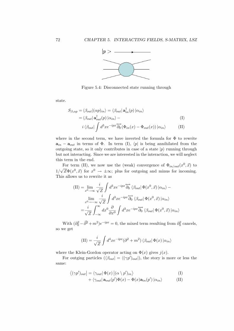
72 CHAPTER 5. INTERACTING FIELDS, S-MATRIX, LSZ
Figure 5.4: Disconnected state running through
state.
Sβ,αp = 〈βout|(αp)in〉 = 〈βout|a†in(p) |αin〉
= 〈βout|a†out(p) |αin〉− (I)
i 〈βout|∫d3xe−ipx
←→∂0 (Φin(x)− Φout(x)) |αin〉 (II)
where in the second term, we have inverted the formula for Φ to rewriteain − aout in terms of Φ. In term (I), 〈p| is being annihilated from theoutgoing state, so it only contributes in case of a state |p〉 running throughbut not interacting. Since we are interested in the interaction, we will neglectthis term in the end.
For term (II), we now use the (weak) convergence of Φin/out(x0, ~x) to1/√ZΦ(x0, ~x) for x0 → ±∞; plus for outgoing and minus for incoming.
This allows us to rewrite it as
(II) = limx0→∞
i√Z
∫d3xe−ipx
←→∂0 〈βout|Φ(x0, ~x) |αin〉−
limx0→−∞
i√Z
∫d3xe−ipx
←→∂0 〈βout|Φ(x0, ~x) |αin〉
=i√Z
∫ ∞−∞
dx0 ∂
∂x0
∫d3xe−ipx
←→∂0 〈βout|Φ(x0, ~x) |αin〉
With (∂20− ~∂2 +m2)e−ipx = 0, the mixed term resulting from ∂2
0 cancels,so we get
(II) =i√Z
∫d4xe−ipx(∂2 +m2) 〈βout|Φ(x) |αin〉
where the Klein-Gordon operator acting on Φ(x) gives j(x).For outging particles (〈βout| = 〈(γp′)out|), the story is more or less the
same: ⟨(γp′)out
∣∣ = 〈γout|Φ(x)∣∣(α \ p′)in⟩ (I)
+ 〈γout|aout(p′)Φ(x)− Φ(x)ain(p′) |αin〉 (II)
5.5. LSZ REDUCTION FORMALISM 73
and again
(II) = limy0→∞
−i√Z
∫d3y 〈γout|T (Φ(y)Φ(x)) |αin〉
←→∂0 e
ip′y−
limy0→−∞
−i√Z
∫d3y 〈γout|T (Φ(y)Φ(x)) |αin〉
←→∂0 e
ip′y
=i√Z
∫d4y 〈γout|T (Φ(y)Φ(x)) |αin〉 (
←−∂ 2y +m2)eip
′y
and we ignore term (I) again, since it does not pertain to the interaction.Applying this reduction algorithm until the in- and out-states have been
reduced to the vacuum, and every time ignoring disconnected parts, givesthe following general result:
〈p1 . . . pn out|q1 . . . qm in〉 =(
i√Z
)n+m ∫ m∏i=1
d4xi
∫ m∏j=1
d4yj× (5.19)
e−iqixi(~∂2xi
+m2) 〈0|T (Φ(y1), . . . ,Φ(yn),Φ(x1), . . . ,Φ(xm)) |0〉 (←−∂ 2yj
+m2)eipjyj
which, although rather long, does look nicely symmetric.
5.5.1 Generating functional
In elementary particle physics, one is mostly interested in S-matrix elements,to calculate scattering amplitudes and eventually cross sections. These canbe related to time-ordered vacuum expectation values, as we have seen:
〈0|T (Φ(x1), . . . ,Φ(xn) |0〉
Vacuum expectation values can be obtained by differentiating the generatingfunctional Z(j):
Z(j) = 〈0|T(exp(i
∫d4xΦ(x)j(x)
)|0〉 (5.20)
since (1i
)n δZ
δj(x1) . . . δj(xn)
∣∣∣∣j=0
= 〈0|T [Φ(x1), . . . ,Φ(xn)] |0〉
Remarks
• The S-matrix, which really is a unitary operator, can be expressed interms of Z(j) as well:
S =: exp(∫
d4y
Φin(y)
[(∂2y +m2)
1√Z
δ
δj(y)
]): Z(j)
∣∣∣∣j=0

74 CHAPTER 5. INTERACTING FIELDS, S-MATRIX, LSZ
(again with normal ordering: annihilation operators to the right ofcreation operators). Exercise: show this.
• The T-product vacuum expectation values are the objectives of ax-iomatic QFT, which postulates spectral conditions, Lorentz/Poincareinvariance and microcausality, and seeks to build up its theories fromthese postulates.
• In perturbation theory, the Fourier transform of 〈0|T (Φ(x1), . . . ,Φ(xn)) |0〉produces poles in the outer momenta, which have to be truncated bythe Klein-Gordon differential operators.
Chapter 6
Invariant PerturbationTheory
6.1 Dyson expansion, Gell-Mann-Low formula
To obtain the Gell-Mann-Low formula, one postulates a unitary operatorU(t) which transforms Φin and Πin into Φ and Π:
Φ(~x, t) = U−1(t)Φin(~x, t)U(t) (6.1)
Π(~x, t) = U−1(t)Πin(~x, t)U(t) (6.2)
This would allow for canonical commutation relations for Φ and Φin. How-ever, the representation of the commutators is unique up to unitary equiv-alence only in QM, where the number of degrees of freedom is finite.
The Hamiltonian H can be split up into two terms, one for the interactionand one for the free part:
H = H0 + Hint
These are all operator-valued functions of field operators; for example, inΦ4-theory, Hint = λ
4!
∫d3xΦ4(~x, t). The Heisenberg equations give the time
developments of Φin and Φ as the equal-time commutators with the relevantHamiltonians:
∂Φin(x)∂t
= i[H0(Φin,Πin),Φin]ET (6.3)
∂Φ(x)∂t
= i[H(Φ,Π),Φ]ET (6.4)
Plugging eq. (6.1) allows us to rewrite the left-hand side of eq. (6.4) as
∂Φ∂t
=∂U−1
∂tΦinU(t) + U−1(t)
∂Φin
∂tU(t) + U−1Φin
∂U∂t
(6.5)
75

76 CHAPTER 6. INVARIANT PERTURBATION THEORY
We know the middle term of eq. (6.5) from eq. (6.3). Sandwiching eq. (6.5)between U(t) and U−1(t) gives:
U(t)∂Φ∂t
U−1(t) = U(t)∂U−1(t)
∂tΦin + i[H0(Φin,Πin),Φin] + Φin
∂U(t)∂t
U−1(t)
Since H is a polynomial in Φ and Π, for which we have eqs. (6.1) and (6.2),respectively, we know
U(t)∂Φ∂t
U−1(t) = iU(t)[H(Φ,Π),Φ]U−1 = i[H(Φin,Πin),Φin]
and so we can conclude that
U(t)∂Φ∂t
U−1(t) = i[H(Φin,Πin),Φin]
Since U is unitary, we know that
UU−1 = 1 and hence U∂tU−1 + (∂tU)U−1 = 0
Using H−H0 = Hint and the above gives
i[Hint(Φin,Πin),Φin] = −[(∂tU(t))U−1(t),Φin] (6.6)
where we could in many cases also write Hint(Φin), since Hint usually doesnot depend on Πin (e.g. Hint = λ
4!
∫d3xΦ4(~x, t)). So, up to constants that
are of no interest to us, we have
(∂tU(t))U−1(t) = −iHint(Φin)
DefiningU(t, t′) := U(t)U−1(t′) (6.7)
we have∂U(t, t′)
∂t= −iHin(Φin(t))U(t, t′) (6.8)
which is solved by
U(t, t′) = T(
exp[−i∫ t
t′dt′′Hint(Φin(t′′))
])(6.9)
where the time-ordering applies to the terms in the exponential series.Exercise: show that this is a solution. Hint: transfer into an integral
equation:
U(t, t′) = 1− i∫ t
t′dt′′Hint(Φin(t′′))U(t′′, t′)
Solve this integral equation by iteration and doing the nested integrationsover a generalized “box”, instead of a “tetrahedron”, using the time ordering

6.1. DYSON EXPANSION, GELL-MANN-LOW FORMULA 77
prescription (of any two fields, the one at the prior time is to the right ofthe one to the left). Alternatively, check that U(t1, t2)U(t2, t3) = U(t1, t3);then, with t1 − t2 = ∆t, the differential equation (eq. (6.8)) is fulfilled.
Note: we avoid, unlike in the case presented by Itzykson & Zuber, U(t) =T(∫ t−∞ . . . ), which, with U(−∞) = t would give Φ(−∞) = Φin.
Now, assume x01 ≥ x0
2 ≥ . . . (if this is not the case, rename your x sothat it is the case). Then,
〈0|T(Φ(x1) . . .Φ(xn)) |0〉 = 〈0|U−1(t)U(t, t1)Φin(x1)U(t1, t2) · · · ×. . .Φin(xn)U(tn, t)U(−t) |0〉
Now taking t→∞ gives
limt→∞〈0|U−1(t)T
(Φin(x1) . . .Φin(xn) exp
−i∫ t
−tdt′Hint(t′)
)U(−t) |0〉
where again the exponential is to be split up into time-ordered parts. Nowconsider
limt→∞
U(−t) |0〉 != λ− |0〉 and limt→∞
U(t) |0〉 != λ+ |0〉
where the λ’s are phase factors resulting from U’s unitarity. The proof ofthese two limits is as follows (compare Bjorken & Drell, vol. II, p. 186):assume
limt→∞〈β|U(−t) |0〉 6= 0
where 〈β| 6= 〈0|. Then take a particle with momentum p out of 〈β|:
〈pαin|U(−t) |0〉 = 〈αin|ain(p)U(−t) |0〉 =
− i∫d3xe−ip0t
′−i~p·~x←→∂
∂x′0〈αin|Φin(−t′, ~x)U(−t) |0〉
and note that Φin(−t′, ~x)U(−t) = U(−t′)Φ(−t′, ~x)U−1(−t′)U(−t). Now lett = t′ →∞; this gives
=√Z 〈αin|U(−t)
=0︷ ︸︸ ︷ain(p) |0〉+i
∫d3xe−ip0t−i~p·~x×
〈αin| (∂tU(−t))Φ(−t, ~x) + U(−t)Φ(−t, ~x)(∂tU−1(−t))U(−t) |0〉
which gives zero. To see this (exercise), use the unitary equivalence andthe equation for ∂tU derived above. Now, since we had assumed it to benonzero, this is a contradiction.

78 CHAPTER 6. INVARIANT PERTURBATION THEORY
Now, we obtain λ−λ∗+ as follows:
1 = 〈0|0〉 = limt→∞〈0|U−1(t)U(t)U−1(−t)︸ ︷︷ ︸
U(t,−t)
U(−t) |0〉 =
λ−λ∗+ 〈0|U(∞,−∞) |0〉 =
λ−λ∗+ 〈0|Texp
[−i∫ ∞−∞
dtHint(Φin(t))]|0〉
which leads us to our final result: the Gell-Mann-Low formula:
〈0|T(Φ(x1) . . .Φ(xn)) |0〉 = (6.10)
〈0|T(Φin(x1) . . .Φin(xn)exp
[−i∫∞−∞ dtHint(Φin(t))
])|0〉
〈0| exp[−i∫∞−∞ dtHint(Φin(t))
]|0〉
This will be our basis when doing perturbation theory. Note that we haveone vacuum |0〉, and that everything is written in terms of free Φin-fields,obtained via the Yang-Feldman equations, acting in Fock space.
6.2 Interaction picture
For completeness’ sake, we will present the interaction picture (also knownas Dirac picture), since many textbooks use it to derive the Gell-Mann-Lowformula. It also offers more insight in the differences between the differentpictures.
6.2.1 Transformation
In the interaction picture, the time dependence is divided over the operatorsand states, unlike in the Heisenberg and Schrodinger pictures. The time de-velopments of those parts of operators that are not explicitly time-dependentare given by H0; those of states by Hint. In the Schrodinger picture,
H = H0 + Hint
At t = 0, all three pictures (Heisenberg, Schrodinger and Dirac) are assumedto coincide. From there, we obtain field operators in the interaction pictureas follows:
Φ0(~x, t) = eiH0tΦ(~x, 0)e−iH0t (6.11)
The Heisenberg analogue is
Φ(~x, t) = eiHtΦ(~x, 0)e−iHt (6.12)
Note that H is time independent in all pictures.
6.2. INTERACTION PICTURE 79
The transformation from the Dirac to the Heisenberg picture,
Φ(~x, t) = eiHte−iH0t︸ ︷︷ ︸eU†(t)
Φ0(~x, t) eiH0te−iHt︸ ︷︷ ︸eU(t)
(6.13)
defines a unitary operator U with the following property:
dU(t)dt
= −ieiH0t(H−H0)eiHt = −ieiH0tHinteiHt (6.14)
Defining H′int := eiH0tHinte−iH0t, we can rewrite this as
dU(t)dt
= −ieiH0tHinte−iH0teiH0teiHt = −iH′inte
iH0te−iHt = −iH′intU(t)
This gives for U(t), like for U(t, t′) before, the following iterative formula:
U(t) = 1− i∫ t
0dt′H′int(t
′)U(t′) (6.15)
From this, one can again obtain the Gell-Mann-Low formula, this time withexpectation values in the vacuum
∣∣0⟩ of the interaction picture, for whichH0
∣∣0⟩ = 0. Note that H′int is a polynomial of field operators of the interac-tion picture.
H0 now is the free Hamiltonian with the mass term 12m
20Φ
20 from the
original (also called “bare”) Lagrangian. This is generally different from theH0 we had before, which gives the time dependence of Φin(x) and has aphysical mass m2. The notation H(m)
0 is also used.Starting again from the T-product vacuum expectation value (vev)
〈0|T(Φ(x1) . . .Φ(xn)) |0〉
and transforming to Φ0 we now want to know the limit (in the weak sense) ofU†(T )
∣∣0⟩ as T goes to ±∞. Shifting the energy such that both H0
∣∣0⟩ = 0and H |0〉 = 0, one has
〈Ψ| eiHT e−iH0T∣∣0⟩ = 〈Ψ| eiHT
∣∣0⟩ =
〈Ψ|0〉⟨0|0⟩
+∫dE 〈Ψ|E〉
⟨E|0⟩eiET
where∫dE 〈Ψ|E〉
⟨E|0⟩eiET → 0 for T → ±∞ by the Riemann-Lebesgue
lemma. From this, we read off
U†(T )∣∣0⟩ |0〉 ⟨0|0⟩ as T → ±∞ (6.16)
which is the Gell-Mann-Low theorem.
80 CHAPTER 6. INVARIANT PERTURBATION THEORY
Using
〈0|0〉 = 1 = limT→∞
⟨0∣∣ U(T )U†(−T )
∣∣0⟩|⟨0|0⟩|2
we can solve for |⟨0|0⟩|2 and obtain
〈0|T(Φ(x1) . . .Φ(xn)) |0〉 = (6.17)
limT→∞
⟨0∣∣T(Φ0(x1) . . .Φ0(xn)exp
[−i∫ T−T H′int(t)dt
]) ∣∣0⟩⟨0∣∣T(exp
[−i∫ T−T H′int(t)dt
]) ∣∣0⟩if we substitute |0〉 according to eq. (6.16) and plug in eq. (6.13) for Φ.
6.2.2 Scattering theory
If one wants to start the discussion of the interaction picture from the be-ginning, one has to introduce scattering states, like in QM. States in theinteraction picture have a time development:
id
dt|ψ〉I = VI(t) |ψ〉I (6.18)
Note that VI was called H′int in the previous section, so
H = H0 + VSch (6.19)
andVI = eiH0tVSche
−iH0t (6.20)
For large positive or negative values of t the interaction is switched off.|ψ(±∞)〉 are time independent and correspond to states in the Schrodingerpicture changing in time with H0.
Naıvely, H and H0 are assumed to have the same spectrum and to actin the same Hilbert space. However, this has to be checked carefully; forexample, the “bare” masses in H0 are not the physical masses appearingin the full H unless one shifts terms in the Hamiltonian H from V to H0
(adding and subtracting mass terms 12(m2
0 −m2)Φ2).Consider stationary states
H0 |φα〉 = Eα |φα〉H∣∣ψ±α ⟩ = Eα
∣∣ψ±α ⟩where the scattering states |ψ±α 〉 serve to construct wave packets which ap-proach |φα〉 for t→ ∓∞ (see figure 6.1); i.e.∫
dα e−iEαtg(α)∣∣ψ±α ⟩→ ∫
dα e−iEαtg(α) |φα〉 (6.21)

6.2. INTERACTION PICTURE 81
Figure 6.1: |φα〉 as t→ ±∞
Formally, this means ∣∣ψ±α ⟩ = Ω(∓∞) |φα〉 or
|φα〉 = Ω†(∓∞)∣∣ψ±α ⟩
with Hermitian Ω(t) = eiHte−iH0t, also called the Møller operator. Now, itis easy to check that
id
dtن(t) = VIن(t)
which is solved by
Ω†(t) = Texp(−i∫ t
0dtVI(t′)
)(where Ω†(0) = 1). Using this Ω, a solution to eq. (6.18) can be written
|ψ(∞)〉I = Ω†(∞)Ω(−∞) |ψ(−∞)〉I︸ ︷︷ ︸=|φα〉
with the S-matrix:
S = Ω†(∞)Ω(−∞) = Texp(−i∫ ∞−∞
dt′VI(t′))
(6.22)
S-matrix elements are given by⟨ψ−β |ψ
+α
⟩= 〈φβ|Ω†(∞)Ω(−∞) |φα〉 = 〈φβ|S |φα〉 (6.23)
Evaluating the S-matrix operator with the Wick theorem will also lead toinvariant pertubation theory and the Feynman rules.

82 CHAPTER 6. INVARIANT PERTURBATION THEORY
Note
If one wants to stay close to QM, one considers the Lippmann - Schwingerequations for |ψ±α 〉:∣∣ψ±α ⟩ = |φα〉+ (Eα −H0 ± iε)−1V
∣∣ψ±α ⟩ (6.24)
which on the face of it looks like a simple identity, but contains the asymp-totes from eq. (6.21).
The evaluation of the S-matrix elements could also be done in timeordered perturbation theory, with “on-shell” intermediate states. To get theright iε prescriptions, one goes to the Lippmann-Schwinger equations andintroduces
〈β|V∣∣ψ+α
⟩= T+
βα fulfilling
T+βα = Vβα +
∫dγVβγT+
γα(Eα − Eγ + iε)
Then, one hasSαβ = δ(β − α)− 2πiδ(Eα − Eβ)T+
βα
The equation for T+βα can be solved by a Neumann series. This results in
a set of rules equivalent to the Feynman rules; later on, we will obtain thedenominators by integrating k0 in the Feynman graphs.
6.2.3 Background field
If one has just an outer field j (also called background field), one has todistinguish |0〉in and |0〉out, but apart from this, the reduction formula workslike the LSZ formalism. One then has to consider
〈0|out T(Φ(x1) . . .Φ(xn)) |0〉in (6.25)
with Φ(x) = U−1(t)Φin(x)U(t)
and U(t) = Texp(−i∫ t
−∞dt′Hint(t′)
)where Hint =
∫d3xΦ(x)j(x). Now, 〈0|out and 〈0|in are related by
〈0|out = 〈0|in S
with
S = Texp(−i∫ ∞−∞
dt′Hint(t′))
(6.26)

6.2. INTERACTION PICTURE 83
Then, (6.25) reads:
limT→∞
〈0|in Texp(−i∫ ∞−∞
dt′Hint(t′))
U−1(T )U(T )U−1(t)×
Φin(x1)U(t1, t2) . . .Φin(xn)U(tn)U−1(T )U(T ) |0〉 =
〈0|in T(
Φin(x1) . . .Φin(xn)exp[−i∫ ∞−∞
dt′Hint(t′)])|0〉in (6.27)
This allows us to discuss the production of n particles out of the vacuumby an outer source (like a current) j(x) switched on at some point in time,and switched off at another. The calculation of the S-matrix transitionamplitudes and of transition probabilities leads to a Poisson distribution.For more on this topic, see Itzykson and Zuber, p. 176.
Since this is a tree-level calculation, without loops, Z 6= 1 is not necessaryhere, so we can caculate the amplitude directly:
〈(p1 . . . pn)out|0〉in = in 〈p1 . . . pn|S |0〉in
with
S = Texp(−i∫ ∞−∞
dt′∫d3x(−j(~x, t′)Φin(~x, t′))
)Splitting into time intervals and using eAeB = eA+B+[A,B]/2, this becomes
S = exp(−i∫d4xΦin(x) j(x)
)exp
(−1
2
∫ ∫d4xd4yθ(x0 − y0)[Φin(x),Φin(y)]j(x)j(y)
)
• Only the a†-part of Φin(x) contributes to the first part; the secondpart is a common factor
exp(−1
2
∫ ∫d4xd4yDR(x− y)j(x)j(y)
)= exp
(−1
2
∫dk|j(k)|2
)
with |j(k)|2 = j(k)j∗(k) = j(k)j(−k).
• S produces a coherent state out of |0〉in.
• The probabilities for producing n particles (see Itzykson & Zuber, p.169)
pn =1n!
(∫dq|j(q)|2
)nexp
(−∫dq|j(q)|2
)form a Poisson distribution.

84 CHAPTER 6. INVARIANT PERTURBATION THEORY
6.3 Haag’s theorem
Assume
(i) translational invariance of the physical vacuum (i.e. the one from theHeisenberg picture)
(ii) “vacuum polarization”, i.e.∣∣0⟩ is not an eigenstate of H
Then, one finds that U(t) does not exist. In other words, the interactionpicture does not exist in QFT.
This is a typical problem with the limit V → ∞. It also appears inthe thermodynamical limit of statistical mechanics (see also R. Haag, LocalQuantum Physics, Springer monographs in physics). The essential point isthat H does not exist in the Fock space HF of the H0-states. H and H0
act in non-equivalent Fock spaces; they exist as different irreducible repre-sentations of the commutation relations in the case of an infinite number ofdegrees of freedom.
Sketch of a proof (see Hegerfeld, Gottingen): define
H∣∣0⟩ = lim
V→∞
∫d3x(H0(x) + Hint(x))
∣∣0⟩ =: |ψ〉
By assumtion (ii), |ψ〉 6= α∣∣0⟩. Now, from the Gell-Mann-Low theorem
|0〉 = limt→±∞
U†(t)∣∣0⟩
〈0| U†(t)∣∣0⟩
we see that∣∣0⟩ has to be translationally invariant, because |0〉 is (assumption
(i)). Hence ⟨0∣∣H(x) |ψ〉 = C (const)
since both⟨0∣∣ and |ψ〉 are translationally invariant. Therefore,
〈ψ|ψ〉 = limV→∞
∫d3x
⟨0∣∣H(x) |ψ〉 =∞
for C 6= 0.Alternatively, one might use that 〈ψ|ψ〉 is finite, so C must be zero, so
〈ψ|ψ〉 = 0, which means that |φ〉 = H∣∣0⟩ = 0, which contradicts assumption
(i).

Chapter 7
Feynman rules, cross section
7.1 Wick theorem
Last chapter, we ended with the Gell-Mann-Low formula, which containedtime ordered products of Φin(x) (Hint is also an expression in Φin). Wewant to rewrite these in terms of c number valued “functions”, which willlater on turn out to be distributions, and normal ordered products, wherethe annihilation operators are placed to the right of the creation operators.The latter do not contribute to vacuum expectation values, but they are stillimportant in time ordered perturbation theory, where they act on Φ0-states.
In this chapter, we will omit the subscript “in” from Φin, and simplywrite Φ. Now, let us start by considering
T(Φ(x1)Φ(x2))
Recall that Φ(x) = Φ−(x) + Φ+(x), where Φ−(x) contains the generationoperator, and Φ+(x) the annihilation operator. Further, assume that x0
1 ≥x0
2. Then,
T(Φ(x1)Φ(x2)) =Φ−(x1)Φ−(x2) + Φ+(x1)Φ+(x2)+Φ−(x1)Φ+(x2) + Φ+(x1)Φ−(x2)
In this expression, the first three terms on the right hand side are alreadywritten in their normal ordered form. The fourth term, Φ+(x1)Φ−(x2), stillhas the annihilation operator to the left of the creation operator. Introducingthe normal ordering, this term has to be removed:
T(Φ(x1)Φ(x2)) =: Φ(x1)Φ(x2) : + Φ+(x1)Φ−(x2)− Φ−(x2)Φ+(x1) =
: Φ(x1)Φ(x2) : +D+(x1 − x2)θ(x01 − x0
2) (7.1)
85
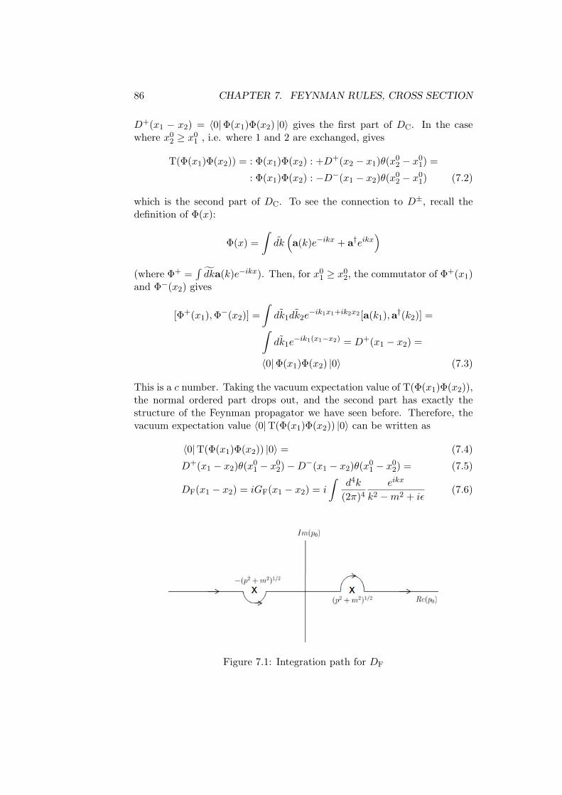
86 CHAPTER 7. FEYNMAN RULES, CROSS SECTION
D+(x1 − x2) = 〈0|Φ(x1)Φ(x2) |0〉 gives the first part of DC. In the casewhere x0
2 ≥ x01 , i.e. where 1 and 2 are exchanged, gives
T(Φ(x1)Φ(x2)) = : Φ(x1)Φ(x2) : +D+(x2 − x1)θ(x02 − x0
1) =
: Φ(x1)Φ(x2) : −D−(x1 − x2)θ(x02 − x0
1) (7.2)
which is the second part of DC. To see the connection to D±, recall thedefinition of Φ(x):
Φ(x) =∫dk(a(k)e−ikx + a†eikx
)(where Φ+ =
∫dka(k)e−ikx). Then, for x0
1 ≥ x02, the commutator of Φ+(x1)
and Φ−(x2) gives
[Φ+(x1),Φ−(x2)] =∫
˜dk1˜dk2e−ik1x1+ik2x2 [a(k1),a†(k2)] =∫
˜dk1e−ik1(x1−x2) = D+(x1 − x2) =
〈0|Φ(x1)Φ(x2) |0〉 (7.3)
This is a c number. Taking the vacuum expectation value of T(Φ(x1)Φ(x2)),the normal ordered part drops out, and the second part has exactly thestructure of the Feynman propagator we have seen before. Therefore, thevacuum expectation value 〈0|T(Φ(x1)Φ(x2)) |0〉 can be written as
〈0|T(Φ(x1)Φ(x2)) |0〉 = (7.4)
D+(x1 − x2)θ(x01 − x0
2)−D−(x1 − x2)θ(x01 − x0
2) = (7.5)
DF(x1 − x2) = iGF(x1 − x2) = i
∫d4k
(2π)4eikx
k2 −m2 + iε(7.6)
Figure 7.1: Integration path for DF

7.1. WICK THEOREM 87
Now, Wick’s theorem states that the general T-product can be reduced tonormal ordered products and vacuum expectation values of T-products ofpairs of Φ:
T(Φ(x1) . . .Φ(xn)) = (7.7): Φ(x1) . . .Φ(xn) : +〈0|T(Φ(x1)Φ(x2)) |0〉 : Φ(x3) . . .Φ(xn) : + · · ·+〈0|T(Φ(x1)Φ(x2)) |0〉 〈0|T(Φ(x3)Φ(xn)) |0〉 : Φ(x5) . . .Φ(xn) : + · · ·+. . . going over all possible contractions
Here, 〈0|T(Φ(x1)Φ(xn)) |0〉 is called the contraction of Φ(x1) and Φ(x2),which is often denoted by Φ(x1)Φ(x2).
The theorem is proven by induction: first, we see that it works for n = 2.Then, we prove that if the theorem holds for n, it also holds for n + 1. Tobegin the proof, let us note that without limitation of generality, we canassume that x0
n+1 is smaller than all other x0, so
T(Φ(x1) . . .Φ(xn)Φ(xn+1)) = T(Φ(x1) . . .Φ(xn))Φ(xn+1)
Now, by assumption, T(Φ(x1) . . .Φ(xn)) can be written in terms of normalordered products. Rewriting Φ(xn+1) as Φ+(xn+1) + Φ−(xn+1), we see thatthe term with Φ+ is already normal ordered. The other term still has to beordered, so Φ−(xn+1) has to be commuted with all the Φ+.
[Φ+(xk),Φ−(xn+1)] =c-number = 〈0| [Φ+(xk),Φ−(xn+1)] |0〉 =〈0|Φ+(xk)Φ−(xn+1) |0〉 = 〈0|Φ(xk)Φ(xn+1) |0〉 =〈0|T(Φ(xk)Φ(xn+1)) |0〉
Commuting with all the Φ+ gives all possible contractions, as Wick’s theo-rem says.
Hint is often assumed to be already normal ordered, e.g. : Φ4(x) :. Other-wise, one would get “self-contractions”, as we will see later when treatingthe path integral formulation.
7.1.1 Φ4-theory
Evaluating interactions in Φ4-theory by Wick’s theorem highlights the cen-tral problem of local QFT: it involves polynomials in GF. If GF is a dis-tribution (like a delta function), taking it to any power other than one is a

88 CHAPTER 7. FEYNMAN RULES, CROSS SECTION
very tricky affair. Consider T(: Φ4(x) :: Φ4(y) :):
T(: Φ4(x) :: Φ4(y) :) = : Φ4(x)Φ4(y) : +
1!(
41
)2
Φ(x)Φ(y) : Φ3(x)Φ3(y) : +
2!(
42
)2 (Φ(x)Φ(y)
)2: Φ2(x)Φ2(y) : +
3!(
43
)2 (Φ(x)Φ(y)
)3: Φ(x)Φ(y) : +
4!(Φ(x)Φ(y)
)4(7.8)
and note that the last three terms have(Φ(x)Φ(y)
), which was shown to
be DF, to some power higher than 1.
7.2 Feynman graphs
7.2.1 Feynman rules in x-space
We want to evaluate the Gell-Mann-Low formula for the T-product vacuumexpectation value of interacting fields from last chapter:
〈0|T[exp(−i∫d4xHint(Φ(x))
)Φ(x1) . . .Φ(xn)] |0〉
〈0|T[exp
(−i∫d4xHint(Φ(x))
)]|0〉
For the sake of simplicity, let us restrict ourselves to real Φ4-theory, whereHint = λ
4! : Φ4 :. Each polynomial T-product vacuum expectation value isevaluated with Wick’s theorem - we can forget about the normal orderedparts, as they do not contribute. The best way of bookkeeping is by meansof graphs: the pionts x1, . . . , xn are to be connected by propagators ΦΦ andvertices:
The first term here is zeroth order in λ; not in the figure are the otherpossible ’disconnected’ combinations. The second term is first order in λ andcomes with a factor of 4!, since there are 4! different possibilities to connectthe lines to the vertex. The third term has a factor of (4! · 4!/2) · 2!: two
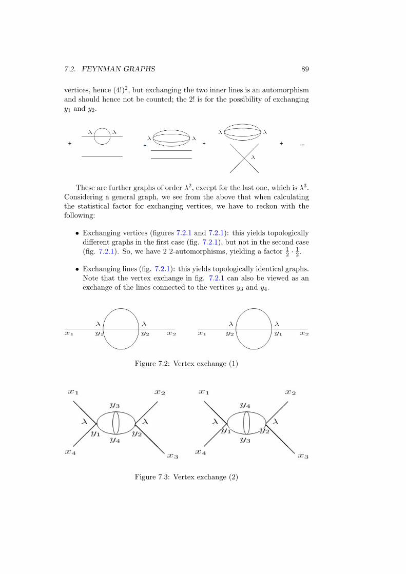
7.2. FEYNMAN GRAPHS 89
vertices, hence (4!)2, but exchanging the two inner lines is an automorphismand should hence not be counted; the 2! is for the possibility of exchangingy1 and y2.
These are further graphs of order λ2, except for the last one, which is λ3.Considering a general graph, we see from the above that when calculatingthe statistical factor for exchanging vertices, we have to reckon with thefollowing:
• Exchanging vertices (figures 7.2.1 and 7.2.1): this yields topologicallydifferent graphs in the first case (fig. 7.2.1), but not in the second case(fig. 7.2.1). So, we have 2 2-automorphisms, yielding a factor 1
2 ·12 .
• Exchanging lines (fig. 7.2.1): this yields topologically identical graphs.Note that the vertex exchange in fig. 7.2.1 can also be viewed as anexchange of the lines connected to the vertices y3 and y4.
Figure 7.2: Vertex exchange (1)
Figure 7.3: Vertex exchange (2)

90 CHAPTER 7. FEYNMAN RULES, CROSS SECTION
Figure 7.4: Line exchange
In case of doubt, counting the number of possible contractions is a wayout. This is more cumbersome than drawing the graphs, but also morereliable.
The factor 14! in λ
4! drops out, since one has to sum over all combinationsof the four lines connecting to the rest of the graph. Similarly, in the Gell-Mann-Low formula, the factor 1
n! in the exponential is cancelled by then! ways to arrange the vertices. In loops, there are combinatorial factorscorrecting the fact that situations are counted several times: one has todivide by the number of automorphisms α(Γ)graph of inner lines and verticeswhich leave the graph unchanged.
Figure 7.5: Automorphisms
The free propagator ΦΦ = 〈0|T(Φin(xi)Φin(xk)) |0〉 has the form
ΦΦ = DF(xi − xk) =∫CF
d4k
(2π)4i
k2 −m2 + iεe−ik(xi−xk) (7.9)
where CF is the Feynman path in the imaginary k0-plane (see fig. 7.1).
Remarks
• for the interacting field Φ,
〈0|T(Φ(x)Φ(y)) |0〉 = ZDF(x− y,m)+∫ ∞>m2
dm′2σ(m′2)DF(x− y,m′)
(7.10)

7.2. FEYNMAN GRAPHS 91
one has a prefactor Z (derivation like in chapter 5).
• We will soon see that in the reduction formula for S-matrix elements,the first part contributes.
• The normal ordering in Hint ensures there are no “tadpole” graphs:
Figure 7.6: Tadpole graphs
There are both connected and “vacuum” graphs in the numerator, butonly vacuum graphs in the denominator.
Let us say there are p vertices in the numerator expansion: s of theseare connected to outer fields, and the other p − s are in vacuum graphs.Decomposing the graph into its connected and vacuum parts,
(−i)p
p!〈0|T(Φin(x1) . . .Φin(xn)Hint(y1) . . .Hint(ys)) |0〉×
p!s!(p− s)!
〈0|T(Hint(ys+1 . . .Hint(yp)) |0〉
we see that the factors of p! cancel each other. This leaves us with
∑p,s
· · · =∑s,p−s
· · · =∑s
1s!〈. . . 〉︸ ︷︷ ︸
no vac. graphs
∑p−s
1(p− s)!
〈. . . 〉︸ ︷︷ ︸vac. graphs
• The denominator cancels the vacuum graphs in the numerator.
We thus obtain the Feynman rules in x-space for Wightman functions〈0|T(Φ(x1) . . .Φ(xn)) |0〉:

92 CHAPTER 7. FEYNMAN RULES, CROSS SECTION
(i) draw all graphs without vacuum parts to some order in the verticess
(ii) a factor DF(x) for each propagator connecting outer points x1, . . . , xnand inner points (vertices) y1, . . . , yn; x is the difference betweenendpoints (here the sign does not matter, but later it will representthe direction of the propagator for charged particles)
(iii) a factor −iλ for each vertex (coupling
(iv) combinatorial factors 1α(Γ)
(v) integrate over the inner points yi:∫d4yi
7.2.2 Feynman rules in momentum space
It is also very useful to Fourier transform the function in the outer xj , i.e.to perform the integrations ∫
d4xje−ikjxj . . .
with the outer momenta kj . Writing down a Fourier representation of DF,where outer points and inner vertices are on the same footing,
DF(x) = i
∫d4x
(2π)4e−ikx
k2 −m2 + iε(7.11)
one can perform the xj and yi integrations and obtain (2π)4δ4(ki, . . . ). Thisgives 4-momentum conservation at the vertices and overall momentum con-servation. We can perform the integrations at the vertices, which leaves uswith one integration per loop and overall momentum conservation. Thisgives the Feynman rules in momentum space:
(i) draw all graphs without vacuum parts to some order in the verticess
(ii) a factor ik2−m2+iε
for each propagator
(iii) a factor −iλ for each vertex
(iv) combinatorial factors 1α(Γ)
(v) integrate over the loop momenta:∫
d4ki(2π)4
, and add a factor (2π)4δ4
for outer momentum conservation

7.2. FEYNMAN GRAPHS 93
Remarks
• We still have disconnected graphs, and in particular lines runningthrough without interacting. This is where the S-matrix comes in,where we have already taken out these cases while applying the reduc-tion formula.
• The vacuum graphs cancel in our case, so here they are not very in-teresting. They contain an overall factor δ4(0µ) =
∫d4xeix
µ·0µ , i.e. aninfinite volume element. This is related to the fact that these graphscan be shifted in space independently of each other. If there are sev-eral disconnected vacuum pieces, they will appear as a sum in theexponential:
〈0| . . . |0〉vac = exp(∑
〈0| connected vacuum pieces |0〉)
Exercise: prove this. Hint: use (a+ b)n/n! =∑k
ak
k!bn−k
(n−k)! .
7.2.3 Feynman rules for complex scalars
For complex scalars, we have
Hint =λ
4(Φ†(x)Φ(x))2 (7.12)
The only propagators we have are of the form
〈0|T(Φ(x)Φ†(y)) |0〉 = DF(x− y) (7.13)
with DF as in eq. (7.9). The other two possibilities give zero:
〈0|T(ΦΦ) |0〉 = 〈0|T(Φ†Φ†) |0〉 = 0
Since we have complex scalar particles here, we need to change the rules:particles propagate from y to x, whereas antiparticles propagate from x toy. Therefore, an arrow is needed to indicate the direction of propagation.Note that this is not related to momentum. See fig. 7.2.3 for a graphicalexplanation. Also, the factor 1
4 cancels the number of possibilities to taketwo Φ† and two Φ out of Hint. Each vertex has two incoming lines, corre-sponding to incoming particles or outgoing antiparticles, and two outgoingones, corresponding to outgoing particles or incoming antiparticles. In mo-mentum space, p0 has to be positive for particles and antiparticles, meaningthe momentum arrows are different from the particle/antiparticle arrows.

94 CHAPTER 7. FEYNMAN RULES, CROSS SECTION
Figure 7.7: Particles and antiparticles with momenta
7.3 Functional relations
As already indicated before, Wightman functions 〈0|T(Φ(x1), . . .Φ(xn)) |0〉with interacting fields Φ can be expanded via the generating functional
Z(j) = 〈0|Texp(i∫d4xΦ(x)j(x)) |0〉 (7.14)
by a series of partial differentiations (1i )n δZδj(x1)...δj(xn) |j=0. In the Gell-Mann-
Low formula, the T-products of interacting fields are expressed by those ofΦin-fields, including the S-matrix Texp[−i
∫∞−∞ d
4yHint(Φin(y))]. Thus,we obtain
〈0|T(Φ(x1) . . .Φ(xn)) |0〉 =(
1i
)n× (7.15)
δδj(x1)...δj(xn) exp[−i
∫d4yHint
(1i
δδj(y)
)] 〈0|T exp
(i∫d4xΦin(x)j(x)
)|0〉
〈0|T exp(i∫d4xΦin(x)j(x)
)|0〉
∣∣∣∣∣∣j=0
This gives vacuum graphs with interaction H(j)int(x) = −Φin(x)j(x), which
exponentiate to
exp(−1
2
∫d4x1d
4x2j(x1)DF(x1 − x2)j(x2))
which, with
Hint
(1i
δ
δj(y)
)=λ
4!
(δ
δj(y)
)4
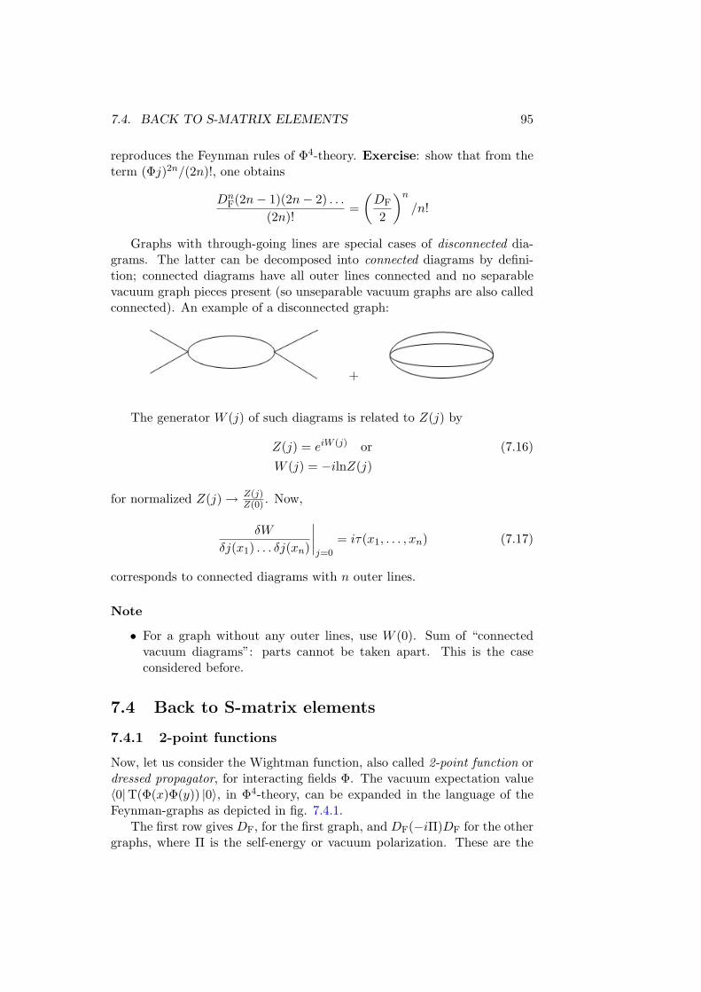
7.4. BACK TO S-MATRIX ELEMENTS 95
reproduces the Feynman rules of Φ4-theory. Exercise: show that from theterm (Φj)2n/(2n)!, one obtains
DnF(2n− 1)(2n− 2) . . .
(2n)!=(DF
2
)n/n!
Graphs with through-going lines are special cases of disconnected dia-grams. The latter can be decomposed into connected diagrams by defini-tion; connected diagrams have all outer lines connected and no separablevacuum graph pieces present (so unseparable vacuum graphs are also calledconnected). An example of a disconnected graph:
+
The generator W (j) of such diagrams is related to Z(j) by
Z(j) = eiW (j) or (7.16)W (j) = −ilnZ(j)
for normalized Z(j)→ Z(j)Z(0) . Now,
δW
δj(x1) . . . δj(xn)
∣∣∣∣j=0
= iτ(x1, . . . , xn) (7.17)
corresponds to connected diagrams with n outer lines.
Note
• For a graph without any outer lines, use W (0). Sum of “connectedvacuum diagrams”: parts cannot be taken apart. This is the caseconsidered before.
7.4 Back to S-matrix elements
7.4.1 2-point functions
Now, let us consider the Wightman function, also called 2-point function ordressed propagator, for interacting fields Φ. The vacuum expectation value〈0|T(Φ(x)Φ(y)) |0〉, in Φ4-theory, can be expanded in the language of theFeynman-graphs as depicted in fig. 7.4.1.
The first row gives DF, for the first graph, and DF(−iΠ)DF for the othergraphs, where Π is the self-energy or vacuum polarization. These are the

96 CHAPTER 7. FEYNMAN RULES, CROSS SECTION
Figure 7.8: Feynman graph representation of 〈0|T(Φ(x)Φ(y)) |0〉
so-called one-particle irreducible graphs, which cannot be further reducedto two-point graphs by cutting just one inner line. The other rows give ageometrical series:
DF +DF(−iΠ)DF +DF(−iΠ)DF(−iΠ)DF + · · · =DF(1 + iΠDF)−1 = (D−1
F + iΠDFD−1F )−1 = (D−1
F + iΠ)−1 (7.18)
For Fourier transformed 2-point functions, with relative and overall momen-tum conservation, this reads[(
i
p2 −m2 + iε
)−1
+ iΠ(p2)
]−1
=i
p2 −m2 −Π(p2) + iε(7.19)
The dressed propagator does not contain a particle pole at p2 = m2 anymore:the denominator now vanishes at p2 = m2 +Π(p2), moving the pole to someother m2. We rename the original m2 → m2
0, called “Lagrange mass” or“bare mass”, and consider the physical mass m2 = m2
0 +Π(m2). This meanswe have to assume a real Π, which will be discussed later. Expanding Π(p2)around p2 = m2, i.e. around the physical mass, we get
i
p2 −m20 − (Π(m2) + (p2 −m2)Π′(m2) + Πrest) + iε
=
i
p2 −m2 − (p2 −m2)Π′(m2) + Πrest + iε=
i(1−Π′(m2))−1
p2 −m2 −Πrest/(p2 −m2) + iε(7.20)
As p2 → m2, Πrest/(p2 −m2) goes to zero, so
limp2→m2
i(1−Π′(m2))−1
p2 −m2 −Πrest/(p2 −m2) + iε=
iZ
p2 −m2 + iε

7.4. BACK TO S-MATRIX ELEMENTS 97
with Z = (1 + Π′(m2))−1. This Z is the same as in the LSZ-formalism fromchapter 5.
7.4.2 General Wightman functions
In general Wightman functions
〈0|T(Φ(x1) . . .Φ(xn)) |0〉
the outer lines of the corresponding Feynman graphs also contain these self-energy subgraphs, each with their own inner lines depending on the orderof perturbation theory to which one goes. So, in the Fourier transformedexpression we have iZ
p2−m2+iεfor p2 → m2.
Figure 7.9: Self-energy of outer lines
Now, let us substitute the Fourier transformed vacuum expectation val-ues into the LSZ reduction formula. With only one incoming q1, we have
i√Z
∫d4x1e
−iq1x1(∂x1 +m2)∫
d4q1(2π)4
eiq1x1F (〈0|T(. . . ) |0〉) =
i√Z
∫d4q1(2π)4
(−q21 +m2)(2π)4δ4(q1 − q1)iZ
q21 −m2 + iε+ Πrest/(q21 −m2)(7.21)
Since the outer particle q1 is on the mass shell, the only pole is at q21 =q21 = m2. Therefore, eq. (7.21) condenses to
√Z. We will discuss ways to
get rid of this remaining factor in the context of renormalization theory, byrenormalizing the field Φ (this is known as wave function renormalization).

98 CHAPTER 7. FEYNMAN RULES, CROSS SECTION
Note
−iΠ(p2) is a divergent quantity in continuum QFT. Consider e.g. the tad-pole contribution:
−iΠtadpole = (−i) λ
(2π)4
∫d4k
i
k2 −m20 + iε
= iλ
(2π)4
∫d4kEucl
−(k2Eucl +m2
0)
The Wick rotation
x0 = −ix4
k0 = ik4
~k = −~kEucl
~x = ~xEucl (7.22)
giveskx = k0x0 − ~k~x = k4x4 + ~kEucl~x = (kx)Eucl (7.23)
Π = λ
∫dk2k2
2dΩ4
1k2 +m2
0
(It is not outer p2-dependent in this case). Introducing a “cut off” Λ2 in thek2-integration, we get
ΠΛ2=λ
22π2 1
(2π)4
∫ Λ2
0dk2 k2
k2 +m2=
λ
16π2
∫ Λ2
0dk2 −m2
∫ Λ2
0
dk2
k2 +m2
︸ ︷︷ ︸
Λ2−m2lnΛ2+m2
m2
In the general case, there also is a p2-dependence, which we will discusslater on in detail. Note that if we want to fix a physical mass (m2), m2
0
becomes cut off dependent by m20 + Π = m2.
7.5 From S-matrix to cross section
7.5.1 Derivation
The S-matrix gives the transition amplitude from in- to out-states:
Sf,p1p1 = 〈αout|p1, p2in〉 (7.24)
for scattering two incoming particles p1 and p2 into a final state |α〉, wherethe in-states have fixed momentum, i.e. are plane waves. Now, we take outthe trivial part of S, where particles are only running through:
S = 1 + iT (7.25)

7.5. FROM S-MATRIX TO CROSS SECTION 99
Making energy-momentum conservation explicit, we have
〈α|T |p1, p2〉 = (2π)4δ4(pf − p1 − p2) 〈α|M |p1, p2〉 (7.26)
In the end, we want to calculate the transition probability. In order to handlethe δ-functions properly, let us, before squaring, introduce wave packets forincoming states:
|p1〉 →∫dp1f1(p1) |p1〉
where |f1(p1)|2 is peaked arbitrarily strongly around p1. Now, we obtain forthe transition probability
Wα←p1,p2 =∫dp1dp2
∫dp′1dp
′2(2π)4δ4(p′1 + p′2 − p1 − p2)×
(2π)4δ4(pf − p1 − p2)f1(p1)f∗1 (p′1)f2(p2)f∗2 (p′2)×〈α|M |p1, p2〉 〈α|M
∣∣p′1, p′2⟩∗With (2π)4δ4(p′1 + p′2 − p1 − p2) =
∫d4x exp(−ix(p′1 + p′2 − p1 − p2)) and∫
dp1f1(p1)eixp1 = f1(x) (and similar for f∗1 , f2 and f∗2 ), this becomes
Wα←p1,p2 =∫d4x|f1(x)|2|f2(x)|2(2π)4δ4(pf − p1 − p2)| 〈α|M |p1, p2〉 |2
Neglecting the variation of the transition amplitude over the wave packetand assuming fi(x) = e−ipixFi(x) with slowly varying Fi(x) (i.e. fi(pi) isstrongly peaked around pi), the transition probability per volume per timeinterval is
dW
dV dt= |f1(x)|2|f2(x)|2(2π)4δ4(pf − p1 − p2)| 〈α|M |p1, p2〉 |2 (7.27)
Now, we still need to normalize the probability current for the positiveenergy solution: it should satisfy the continuity equation
if∗(x)←→∂ µf(x) ∼ 2pµ|f(x)|2 (7.28)
where the f fulfill the Klein-Gordon equation. The ∼-symbol is used here,because f(p) is strongly peaked, so f(x) is almost a plane wave.
Now, when we go into actual experiment, we have a target, at rest in thelaboratory’s frame, which is being bombarded with particles. In the target,the number of particles per volume element is:
dn2
dV= 2p0
2|f2(x)|2 = 2m2|f2(x)|2 (7.29)
The incident flux of bombarding particles is given by
|~p1|p01︸︷︷︸
velocity
× 2p01|f1(x)|2︸ ︷︷ ︸density
= 2|~p1||f1(x)|2 (7.30)

100 CHAPTER 7. FEYNMAN RULES, CROSS SECTION
7.5.2 Scattering amplitudes and cross sections: an example
Consider two scalar fields, one complex (Φ) and one real (φ), with the fol-lowing Lagrangian:
L =12∂µφ∂
µφ+ ∂µΦ∗∂µΦ− V (Φ,Φ∗, φ) (7.31)
where
V (Φ,Φ∗, φ) =12m2φ2 +m2
ΦΦ∗Φ + µmΦ∗Φφ+λ
4(Φ∗Φ)2 (7.32)
Remember the formulas for Φ and φ:
Φ(x) =∫dkaΦ(k)e−ikx + b∗Φ(k)eikx
(7.33)
φ(x) =∫dka(k)e−ikx + a∗(k)eikx
(7.34)
Exercise: inserting this into the LSZ-reduction formula, the
(i) outgoing (aΦ) particles produce a factor∫eipx × (~∂2
x +m2) 〈0|T(. . .Φ(x) . . . ) |0〉
(ii) incoming (aΦ) particles produce a factor∫e−ipx × (~∂2
x +m2) 〈0|T(. . .Φ†(x) . . . ) |0〉
(iii) outgoing (bΦ) antiparticles produce a factor∫eipx × (~∂2
x +m2) 〈0|T(. . .Φ†(x) . . . ) |0〉
(iv) incoming (bΦ) antiparticles produce a factor∫e−ipx × (~∂2
x +m2) 〈0|T(. . .Φ(x) . . . ) |0〉
We want to calculate the scattering amplitude for particles/antiparticles ofΦ-type to order µ2 ∼ λ (this is our choice of parameters). Fig. 7.5.2 repre-sents particle-particle scattering; for antiparticle-antiparticle scattering, onehas the same graphs with reversed charge transport directions. Fig. 7.5.2represents particle-antiparticle scattering.
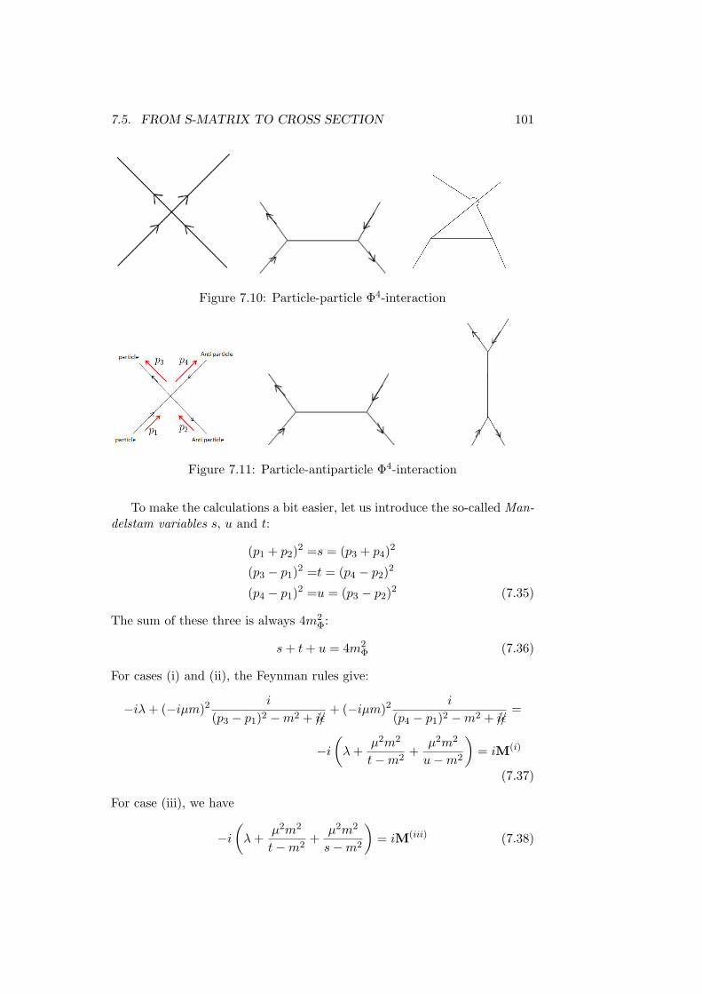
7.5. FROM S-MATRIX TO CROSS SECTION 101
Figure 7.10: Particle-particle Φ4-interaction
Figure 7.11: Particle-antiparticle Φ4-interaction
To make the calculations a bit easier, let us introduce the so-called Man-delstam variables s, u and t:
(p1 + p2)2 =s = (p3 + p4)2
(p3 − p1)2 =t = (p4 − p2)2
(p4 − p1)2 =u = (p3 − p2)2 (7.35)
The sum of these three is always 4m2Φ:
s+ t+ u = 4m2Φ (7.36)
For cases (i) and (ii), the Feynman rules give:
−iλ+ (−iµm)2i
(p3 − p1)2 −m2 + iε//+ (−iµm)2
i
(p4 − p1)2 −m2 + iε//=
−i(λ+
µ2m2
t−m2+
µ2m2
u−m2
)= iM(i)
(7.37)
For case (iii), we have
−i(λ+
µ2m2
t−m2+
µ2m2
s−m2
)= iM(iii) (7.38)

102 CHAPTER 7. FEYNMAN RULES, CROSS SECTION
So, exchanging (i) and (iii) comes down to exchanging s and u. Note thatwe do not need the iε-prescription here, since we do not reach the poles.
Note
Amplitudes are real analytic in two of the three Mandelstam variables; this iscalled Mandelstam analyticity and has been studied extensively in the 1960s.At that time perturbation theory in the case of the strong interactions, whattoday is the field of quantum chromodynamics (QCD), was considered to bejust a guideline to analytic properties of amplitudes, whereas the unitarityof the S-matrix, especially in the 2-2 channel, was considered to be mostimportant. See “The analytic S-matrix” by Eden, Landshoff, Olive andPolkinghorne (and bootstrap ideas by Chew) for more details.
The amplitudes M can be used to calculate cross sections with the for-mulas explained before; in our case, this is particularly simple, since we haveonly tree-level graphs, i.e. without loops. See the literature on elementaryparticle physics for more on this topic.
We finally obtain our cross section by calculating
(transition probability) / (incident flux × target density):
dσ = (2π)4δ4(pf − p1 − p2)1
4m2p1| 〈f |M |p1, p2〉 |2
For an n-particle final state in Lorentz covariant notation, this is:
dσn←2 =1
4[(p1 · p2)2 −m21m
22]1/2
∫dp3 . . . dpn+1 (7.39)
(2π)4δ4(p1 + p2 − p3 + p4 − · · · − pn+2)| 〈p3, . . . pn+2|M |p1, p2〉 |2
For the fermion case, we also need to sum over, or fix, the spin, but apartfrom that, the result is the same (this is different from Itzykson and Zuber’sbook, where the 2m factor in uu is not introduced; this will be discussedlater). For the case with n identical outgoing particles, there will also be acombinatorial factor of 1/n!.
7.5.3 The optical theorem
Because of probability conservation, S = 1 + iT is unitary:
S†S = 1 (7.40)
so, −i(T−T†) = T†T. Consider
〈k1, k2|T†T |k1, k2〉 =∑n
n∏i=1
∫dqi 〈k1, k2|T† |qi〉 〈qi|T |k1, k2〉
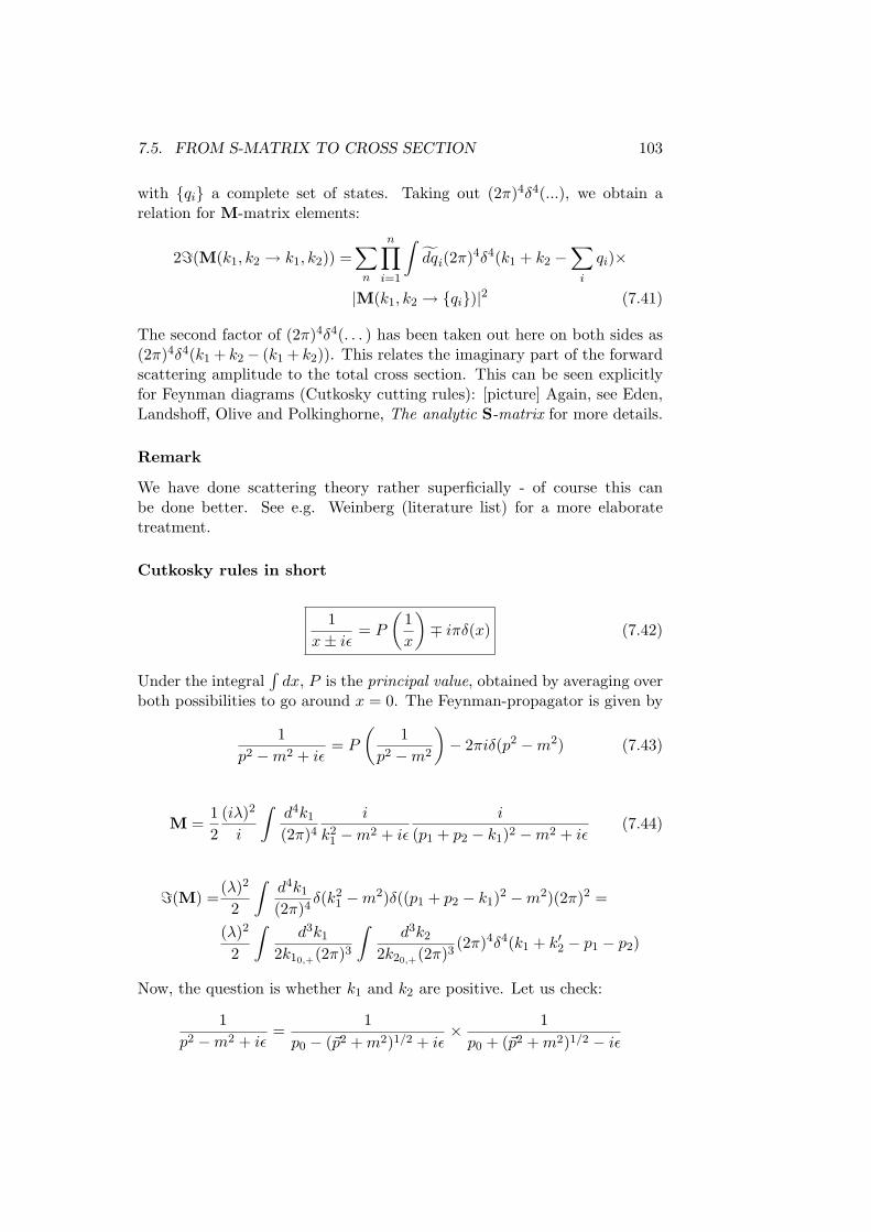
7.5. FROM S-MATRIX TO CROSS SECTION 103
with qi a complete set of states. Taking out (2π)4δ4(...), we obtain arelation for M-matrix elements:
2=(M(k1, k2 → k1, k2)) =∑n
n∏i=1
∫dqi(2π)4δ4(k1 + k2 −
∑i
qi)×
|M(k1, k2 → qi)|2 (7.41)
The second factor of (2π)4δ4(. . . ) has been taken out here on both sides as(2π)4δ4(k1 + k2− (k1 + k2)). This relates the imaginary part of the forwardscattering amplitude to the total cross section. This can be seen explicitlyfor Feynman diagrams (Cutkosky cutting rules): [picture] Again, see Eden,Landshoff, Olive and Polkinghorne, The analytic S-matrix for more details.
Remark
We have done scattering theory rather superficially - of course this canbe done better. See e.g. Weinberg (literature list) for a more elaboratetreatment.
Cutkosky rules in short
1x± iε
= P
(1x
)∓ iπδ(x) (7.42)
Under the integral∫dx, P is the principal value, obtained by averaging over
both possibilities to go around x = 0. The Feynman-propagator is given by
1p2 −m2 + iε
= P
(1
p2 −m2
)− 2πiδ(p2 −m2) (7.43)
M =12
(iλ)2
i
∫d4k1
(2π)4i
k21 −m2 + iε
i
(p1 + p2 − k1)2 −m2 + iε(7.44)
=(M) =(λ)2
2
∫d4k1
(2π)4δ(k2
1 −m2)δ((p1 + p2 − k1)2 −m2)(2π)2 =
(λ)2
2
∫d3k1
2k10,+(2π)3
∫d3k2
2k20,+(2π)3(2π)4δ4(k1 + k′2 − p1 − p2)
Now, the question is whether k1 and k2 are positive. Let us check:
1p2 −m2 + iε
=1
p0 − (~p2 +m2)1/2 + iε× 1p0 + (~p2 +m2)1/2 − iε
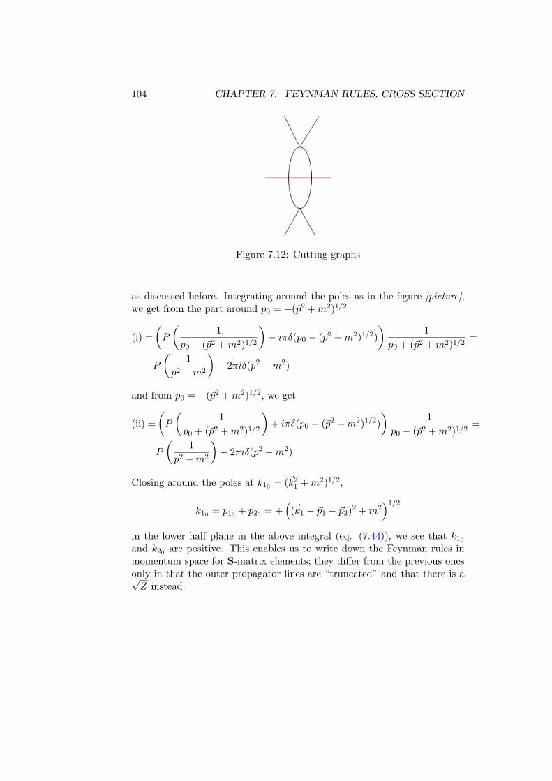
104 CHAPTER 7. FEYNMAN RULES, CROSS SECTION
Figure 7.12: Cutting graphs
as discussed before. Integrating around the poles as in the figure [picture],we get from the part around p0 = +(~p2 +m2)1/2
(i) =(P
(1
p0 − (~p2 +m2)1/2
)− iπδ(p0 − (~p2 +m2)1/2)
)1
p0 + (~p2 +m2)1/2=
P
(1
p2 −m2
)− 2πiδ(p2 −m2)
and from p0 = −(~p2 +m2)1/2, we get
(ii) =(P
(1
p0 + (~p2 +m2)1/2
)+ iπδ(p0 + (~p2 +m2)1/2)
)1
p0 − (~p2 +m2)1/2=
P
(1
p2 −m2
)− 2πiδ(p2 −m2)
Closing around the poles at k10 = (~k21 +m2)1/2,
k10 = p10 + p20 = +((~k1 − ~p1 − ~p2)2 +m2
)1/2
in the lower half plane in the above integral (eq. (7.44)), we see that k10
and k20 are positive. This enables us to write down the Feynman rules inmomentum space for S-matrix elements; they differ from the previous onesonly in that the outer propagator lines are “truncated” and that there is a√Z instead.

Chapter 8
Path integral formulation ofQFT
So far, we have studied QFT in the canonical formalism with operator-valuedfields, in the Heisenberg representation. Richard Feynman has formulatedanother representation of both QM and QFT, which is very intuitive anddoes not use operators. Its mathematical status, however, is still in develop-ment. This method is particularly powerful if one wants to quantize gaugetheories - this is why it is necessary to discuss it - and it also allows oneto derive the Feynman rules very easily, and to discuss problems beyondperturbation theory, although we will not go into the latter here.
8.1 Path integrals in QM
The path integral formulation of QM centers around the transition ampli-tude for a QM particle from a position x(t) at a time t to a position x′(t′)at time t′. It starts from the Heisenberg picture, where the time dependentoperators X(t) and P(t) have their respective eigenvectors |x(t)〉 and |p(t)〉,with time developments
X(t) = eiH(t−t0)/~X(t0)e−iH(t−t0)/~ (8.1)
|x(t)〉 = eiH(t−t0)/~ |x(t0)〉 (8.2)
and similarly for P and p. The factors of ~ have been reinserted here forclarity. Note that the sign in eq. (8.2) is opposite to that of the Schrodingerequation. Note also that this equation describes a transition in time, whilethe position does not change. Finally, in eq. (8.1), X(t0) = XS; in theSchrodinger picture, t0 is usually taken to be 0.
Let us start at the end of our discussion of the path integral formulation,
105

106 CHAPTER 8. PATH INTEGRAL FORMULATION OF QFT
with the result:
⟨x′(t′)|x(t)
⟩=∫DxDp exp
[i
∫ t′
tdτ
p(τ)
dx
dτ−H(p, x)
/~
](8.3)
Here,∫Dx is a path integral, in mathematical circles know as functional
integral, an integral over all possible paths x(τ) connecting x and x′, withx(t) = x and x(t′) = x′.
Figure 8.1: Integrate over all possible paths
∫Dp does not have boundary conditions, since the problem asks for the
transition amplitude between positions, but not between momenta. (As asmall aside: note that the exponent is just the classical action times i/~.)
After discretization of the time integral, it becomes a product of integralsat τ1, τ2, . . . over x(τ1), x(τ2), . . . :
Figure 8.2: Discretization of the time integral
∫Dx exp
(∫dτ . . .
)→∏i
∫ ∞−∞
dx(τi)
Defining δτ := τi−τi−1, one eventually has to take the limit δτ → 0, which ismathematically demanding. Obviously, the integral over Dx does not needto be evaluated at the endpoints, since these are fixed.

8.1. PATH INTEGRALS IN QM 107
Now, let us derive this result. From the canonical formalism, we havethe following formula:⟨
x′(t′)|x(t)⟩
=⟨x′∣∣ e−iH(t′−t)/~ |x〉 (8.4)
where |x〉 is a Schrodinger state. Decomposing the interval into N bits,t′ − t = Nε, gives
〈xN | e−iHε/~ |xN−1〉 〈xN−1| e−iHε/~ |xN−2〉 〈xN−2| . . .. . . |x1〉 〈x1| e−iHε/~ |x0〉
where xN = x′ and x0 = x, and H = P2
2m + V (X). Consider one of thesematrix elements, to order ε:
〈xk+1| e−iHε/~ |xk〉 = 〈xk+1| 1−iH~ε+ . . . |xk〉 =
〈xk+1|xk〉 − iε∫
dpk2π~
V
(xk+1 + xk
2
)〈xk+1|pk〉 〈pk|xk〉+
〈xk+1|pk〉⟨pk
∣∣∣∣P2
2m
∣∣∣∣xk⟩+ · · · = (8.5)∫dpk2π~
[1− iε
~
(p2k
2m+ V
(xk+1 + xk
2
))]exp
(ipk~
(xk+1 − xk))
+ . . .
Note: for more complicated X/P-mixed operators one needs Weyl or-dering, a symmetrization of the operator sequence in X/P; see Peskin& Schroder, p. 281 for more on this topic. Note that the argument inV (xn+1+xn
2 ) is written like this for cosmetic reasons; we could just as wellhave written xn, since in the end, the limit N → ∞ will be taken. Contin-uing our derivation, let us define
θ(ε) =∫
dpk2π~
exp(− iε
~
(p2k
2m+ V
(xk + xk+1
2
)− pk
xk+1 − xkε
))(8.6)
which is the right hand side of eq. (8.5) to order O(ε). Multiplying all θ’sand taking the limit ε→ 0, we have
⟨x′(t′)|x(t)
⟩=∫DxDp exp
[i
∫ t′
tdt
(px−H(p, q)
~
)](8.7)
with x(t) = x and x(t′) = x′. This limit is of course accompanied by somehigher-level mathematics. The naıve expression, however, has to be basedon the discretized version we started from. Concretely, for physicists, thismeans that in QFT, numerical lattice calculations are an adequate way toapproach this integral. Note that the continuous and differentiable functionsare a dense set of measure zero in the functional integral.

108 CHAPTER 8. PATH INTEGRAL FORMULATION OF QFT
The dpk-integration in eq. (8.6) can be performed: it is just a Gaussianintegral, here restricted to one dimension for simplicity. It is solved bycompleting the square:
−p2kε
2m+ pk(xk − xk+1) =
− 12
[p2k
mε− 2pk(xk − xk+1) +
(xk − xk−1)2
εm
]+
12m
(xk − xk−1)2
ε=
−p′k
2
2ε
m+
12m
(xk − xk−1)2
ε
with p′k := pkm −
xk−xk+1
ε . Using the standard Gaussian integral,∫ ∞−∞
dxe−αx2
=(πα
)1/2(8.8)
we can perform the p′k-integral. The first part becomes∫ ∞−∞
dp′k2π~
exp(−1
2iε
~mp′2k
)=
12π~
∫ ∞−∞
dye−y2/2 =
12π~
√2π~miε
where y = p′k√iε/~m. Note that due to the presence of
√i in the conver-
sion from p′k to y, this substitution constitutes a 45-degree rotation of theintegration path:
So, the final result, the product of all the separate integrals, is
N−1∏j=1
∫dxj
(√m
iε~2π
)Nexp
(i
N∑i=1
ε
m
2(xi − xi−1)2
ε2− V (xi)
/~
)
which, after taking ε to zero and N to infinity, becomes:
⟨x(t)|x′(t′)
⟩=∫Dx exp
(i
∫ t′
tdτL(x, x)/~
)(8.9)

8.1. PATH INTEGRALS IN QM 109
with singular integration measure (∼ ε−N/2) and Lagrangian density L =mx2
2 − V (x).The x-space path integral is less general (namely only for H quadratic
in p) than the first version, but for our purpose, we can settle for this one.
Remarks
• For 〈x′(t′)|T(O1(t1)O2(t2) . . . ) |x(t)〉, the operators O1,O2, . . . actin the time slices around t1, t2, . . . . Then, 〈x(t1)|O1(t1) |x(t′1)〉 =O1(x(t1))δ(t1 − t′1) where O1 is a function. Thus, we obtain time-ordering in the path integral, which is decomposed into time slices.This remark is also important if the potential has the shape of a ma-trix in more complicated settings.
• The oscillating behaviour of the Feynman exponential, which makesthe convergence of the integral a more subtle affair, can be avoided ifwe go to imaginary, or Euclidean, time (t = x0 = −ix4 = −itE). Thisso-called Wick rotation helps us to define certain expressions properly.Of course, one has to rotate back at the end of the calculation .
8.1.1 Vacuum expectation values
When going to QFT, we will be interested in vacuum expectation values (cf.correlation functions in statistical physics). Let us briefly investigate themhere:
〈0|T(x(t1) . . .x(tn)) |0〉 =?
Let us start from
〈xT (T )|T(x(t1) . . .x(tn)) |x−T (−T )〉 =∫ xT
x−T
Dxx(t1) . . . x(tn)× (8.10)
exp(−∫dτe
(mx2
2+ V (x)
))where τe stands for Euclidean (Wick-rotated) time. Now,
|x−T (−T )〉 = e(−T )H |x−T (0)〉 =∑n
|n〉 〈n|x−T 〉 e−EnT
where |x−T (0)〉 is also written |x−T 〉, and is a Schrodinger vector, which att = 0 coincides with the corresponding Heisenberg vector. When T is large,only the ground state contributes. Then, eq. (8.10) becomes
= 〈xT (0)|0〉 〈0|T(x(t1) . . .x(tn)) |0〉 〈0|x−T (0)〉 e−2E0T
Dividing by 〈xT (T )|x−T (−T )〉, like in the Gell-Mann-Low formula, removesthe outer parts, leaving
〈0|T(x(t1) . . .x(tn)) |0〉 = limT→∞
ZT
∫ xT
x−T
Dxx(t1) . . . x(tn)e−S (8.11)

110 CHAPTER 8. PATH INTEGRAL FORMULATION OF QFT
where ZT =∫ xT
x−TDx e−S and S =
∫dτe(mx
2
2 + V (x)).
Remarks
• Note the similarity with the thermal average in statistical mechanicswith the Boltzmann weight e−βH .
• x±∞ is in general not a fixed value; taking the Gell-Mann-Low quo-tient, the final result should not depend on it.
• The Feynman-Kac formula: limT→∞ log 〈xT (T )|x−T (−T )〉 /(−2T ) =E0. Exercise: derive this result.
8.2 Path integrals in QFT
8.2.1 Framework
Consider real scalar field theory, with L = 12∂µΦ∂
µΦ − V (Φ), where V (Φ)could for example be m2
2 Φ2 + λ4Φ4. Now, Φ(~x, t) substitutes xi(t) as we go
to infinitely many degrees of freedom. The following correspondences hold:
QM QFT
• Xi(t) (Heisenberg picture)
• |xi(t)〉 state vectors withXi(t) |xi(t)〉 = xi(t) |xi(t)〉
• boundary conditions
• Φ(~x, t) Heisenberg operator
• Fock space (Φ-eigenvectorstates; coherent states)
• vacuum state |0〉 for t →±∞
|0〉 is unique only without outer fields (“currents”). With outer fields (or“currents”), as we have seen before in the generating functional Z(j), wehave an extra term Lj in the Lagrangian density: Lj = j(x)Φ(x), wherej → 0 for large ~x and t. This implies that |Ωt→−∞〉 6= |Ωt→∞〉 and |0〉out 6=|0〉in.
Going from xi to Φ, our path integral will run over fields Φ, and mo-mentum fields Π, where the latter are given by
Π(x) =∂L
∂(∂0Φ)= ∂0Φ = ∂tΦ (8.12)
Now, the Φ- and Π-integrals become:∫DΦ→ lim
∫ ∏i,j
dΦ(~xi, τj) = lim∫ ∏
k
dΦk
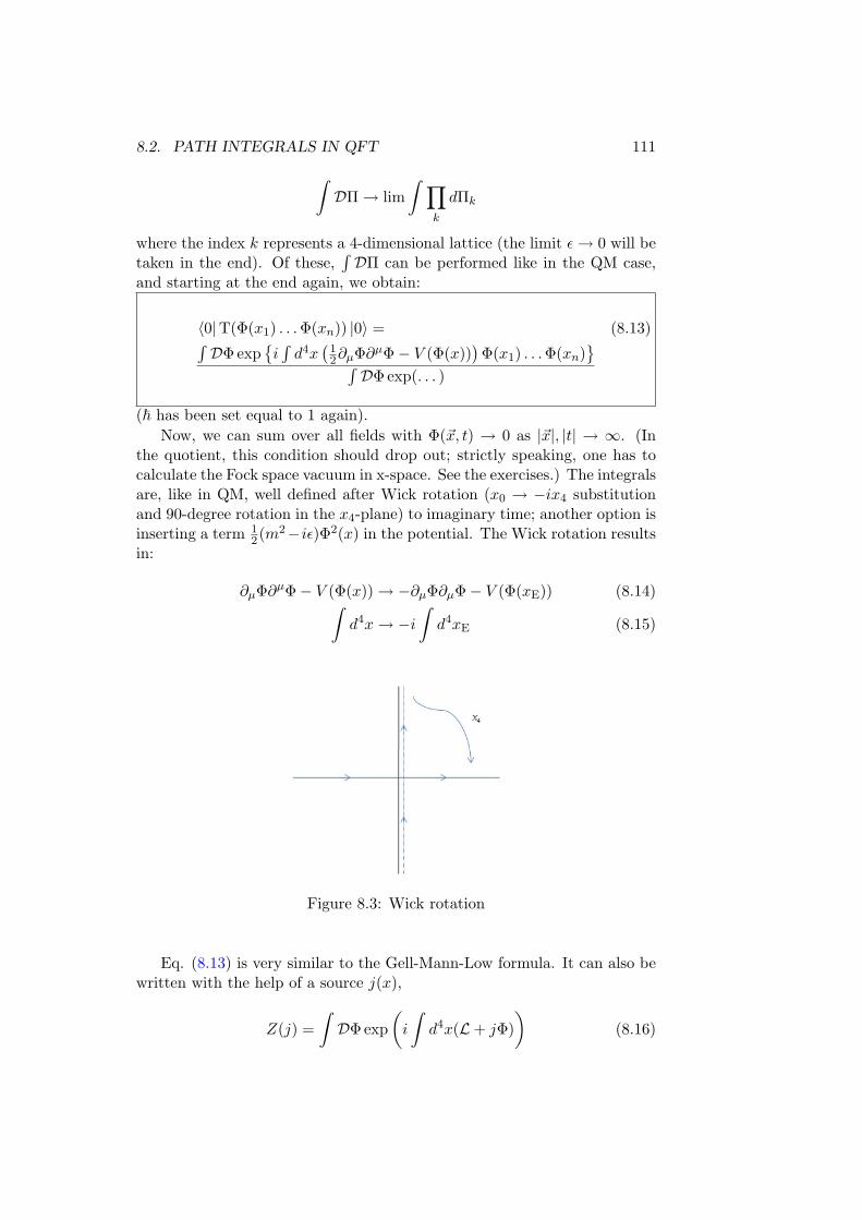
8.2. PATH INTEGRALS IN QFT 111∫DΠ→ lim
∫ ∏k
dΠk
where the index k represents a 4-dimensional lattice (the limit ε→ 0 will betaken in the end). Of these,
∫DΠ can be performed like in the QM case,
and starting at the end again, we obtain:
〈0|T(Φ(x1) . . .Φ(xn)) |0〉 = (8.13)∫DΦ exp
i∫d4x
(12∂µΦ∂
µΦ− V (Φ(x)))Φ(x1) . . .Φ(xn)
∫DΦ exp(. . . )
(~ has been set equal to 1 again).Now, we can sum over all fields with Φ(~x, t) → 0 as |~x|, |t| → ∞. (In
the quotient, this condition should drop out; strictly speaking, one has tocalculate the Fock space vacuum in x-space. See the exercises.) The integralsare, like in QM, well defined after Wick rotation (x0 → −ix4 substitutionand 90-degree rotation in the x4-plane) to imaginary time; another option isinserting a term 1
2(m2−iε)Φ2(x) in the potential. The Wick rotation resultsin:
∂µΦ∂µΦ− V (Φ(x))→ −∂µΦ∂µΦ− V (Φ(xE)) (8.14)∫d4x→ −i
∫d4xE (8.15)
Figure 8.3: Wick rotation
Eq. (8.13) is very similar to the Gell-Mann-Low formula. It can also bewritten with the help of a source j(x),
Z(j) =∫DΦ exp
(i
∫d4x(L+ jΦ)
)(8.16)

112 CHAPTER 8. PATH INTEGRAL FORMULATION OF QFT
which gives
〈0|T(Φ(x1) . . .Φ(xn)) |0〉 =1
(i)nZ(0)δnZ(j)
δj(x1) . . . δj(xn)
∣∣∣∣j=0
(8.17)
where the variational derivative provides factors iΦ(xi). Note: the normal-ization of
∫DΦ is often chosen to give Z(0) = 1.
8.2.2 QFT path integral calculations
Deriving eq. (8.13) in a discretized version, like we did for the QM case,involves a multi-component version of the standard Gaussian integral, eq.(8.8):
I(A, b) =N∏i=1
∫ ∞−∞
dΦi exp(−1
2ΦiAikΦk + biΦi
)(8.18)
We diagonalizeA by an orthogonal transformation O, whose Jacobi-determinantis 1. Then, we have
I(a, b′) =N∏i=1
∫ ∞−∞
dΦ′i exp(−1
2Φ′iaiiΦ
′i + b′iΦ
′i
)
Completing the square, we rewrite −12Φ′iaiΦ
′i + b′iΦ
′i into −1
2ai(Φ′i −
b′iai
)2 +12b′i
1aib′i, which gives
I(a, b′) =N∏i=1
√2πai
exp(
12b′i
1aib′i
)= (2π)N/2
1(detA)1/2
exp(
12bTA−1b
)where the second step is the result of rotating back. So, in the end, we areleft with
I(A, b) =(2π)N/2
(detA)1/2exp
(12bTA−1b
)= I(A, 0) exp
(12bTA−1b
)(8.19)
Observe that (2π)N/2
(detA)1/2 = I(A, 0).Differentiation with respect to bi produces vacuum expectation values:
∂
∂bi
∂
∂bkI(A, b)
∣∣∣∣b=0
= I(A, 0)× (A−1)ik︸ ︷︷ ︸2-point function
(8.20)
Let us apply this to the Z(j) from above, at first without interaction:
L = ∂µΦ∂µΦ +m2
2Φ2 (8.21)

8.2. PATH INTEGRALS IN QFT 113
Note that this is the Euclidean, i.e. rotated, form. With this L,
ZE0 (j) = ZE
0 (0) exp(
12
∫j(x)(−∂2
E +m2)−1xx′j(x
′)d4xEd4x′E)
(8.22)
For comparison: in the Minkowski metric, it looks like this:
Z0(j) =Z0(0) exp(− 1
2i
∫j(x)(∂2 +m2 − iε)−1
xx′j(x′)d4xd4x′
)=
Z0(0) exp(−1
2
∫j(x)DF(x− x′)j(x′)d4xd4x′
)In the Euclidean metric, the calculation is easier due to the absence of thei-factors. It is easy to check that
〈0|T(Φ(x1)Φ(x2)) |0〉 =1i2
δ2Z(j)δj(x1)δj(x2)
∣∣∣∣Z(0)
= DF(x1 − x2)
Remarks
• This can also be performed in the Fourier transformed form:
SE0 =
12
∫d4p
(2π)4(Φ(p)(p2 +m2)Φ(−p)− j(p)Φ(−p)− j(−p)Φ(p)
)with j(−p) = j∗(p) and Φ(−p) = Φ∗(p), since j and Φ are real. Re-defining
Φ(p) = Φ′(p) + (p2 +m2)−1j(p)
(i.e., completing the square) gives
ZE0 (j) = ZE
0 (0) exp
(12
∫d4p
(2π)4j(p)j(−p)p2 +m2
)
• WithW0(j) =
12
∫dxdx′j(x)(iDF)j(x′)
we obtain the following relation for Z and W :
Z0(j)Z0(0)
= eiW0(j)(= e−W
E(j))
where the factor iDF generates the connected 2-point functions; thiswill be generalized later on. This relation resembles the one betweenthe partition function and the free energy in thermodynamics. Note,by the way, that Z and W have been exchanged in the text by Ramond(see literature list).
114 CHAPTER 8. PATH INTEGRAL FORMULATION OF QFT
8.2.3 Perturbation theory
The perturbative approach to path integrals will, again, be introduced inthe Euclidean notation. We will be dealing with a potential V (Φ), whichcan be written as
VE(Φ)→ VE
(δ
δj
)(8.23)
where the differentiation is acting on the generating functional ZE0 (j). (For
example, λ4!Φ
4 → λ4!
(δ
δj(x)
)4.) Let us start with
〈0|T(Φ(x1) . . .Φ(xn)) |0〉 =1
Z(0)δnZ(j)
δj(x1) . . . δj(xn)
∣∣∣∣j=0
(8.24)
Now, expand the exponential in the path integral for Z(j) in powers of V (Φ)and act on Z0(j) with V ( δδj ) as discussed before. Note that also the δ
δj(xi)
in eq. (8.24) act on Z0(j). The δδj of the outer Φ and vertex Φ pairwise
remove the j-legs of exp(12
∫jDFj). Division by Z(0) eliminates the vacuum
graphs (n.b.: Z0(0) is not the same as Z(0)). For example, a vertex withV = λ
4!Φ4 requires 4 propagators (permutation gives the factor of 4!). Also,
several vertices, each with their factor of 1n! , can be permuted and require
a combinatorial factor. From all this, the usual rules for Feynman graphsemerge again:
(i) only graphs with outer lines (no vacuum graphs)
(ii) DF for inner and outer propagators
(iii) λ and∫d4y for each vertex
(iv) combinatorial factors
Exercise: complex scalar fields:
Z(j, j) =∫DΦ exp(−Φ†AΦ + V (Φ)− jΦ− Φ†j)
Here, Φ is a complex vector (with index x). Rewriting it as Φ = (Φ1 +iΦ2)/
√2 reduces the problem to two real fields Φ1,2. DΦ = DΦ1DΦ2, or,
more elegantly, DΦDΦ† with independent Φ,Φ†. A = −∂2E +m2 in case of
the free complex Klein-Gordom field, and Z0(j, j) = exp−jA−1j). Derivethe Feynman rules for V (Φ) = λ (Φ†Φ)2
4 .
8.2. PATH INTEGRALS IN QFT 115
Recapitulation
In the path integral formulation of QFT, vacuum expectation values of timeordered products of operators are calculated with the following formula:
〈0|T(Φ(x1) . . .Φ(xn)) |0〉 =1
Z(0)δnZ(j)
δj(x1) . . . δj(xn)
∣∣∣∣j=0
(8.25)
where
Z(j) = e−V ( δ
δj)Z0(j) and
Z0(j) = Z0(0) exp(
12
∫dxdx′j(x)DF(x− x′)j(x′))
)(8.26)
• Z0(0) drops out in eq. (8.25).
• Vacuum diagrams are cancelled by the division by Z(0).
• The Feynman rules are the same as those obtained in the frameworkof canonical quantization.

116 CHAPTER 8. PATH INTEGRAL FORMULATION OF QFT

Chapter 9
Classification of finiterepresentations of theLorentz group
9.1 Classification of Lorentz transformations
The Lorentz transformations, like the rotations, form a non-commutative,also called non-Abelian, group, which, however, is non-compact. They arerepresented by matrices Λ with the following property:
ΛT gΛ = g (9.1)
The group operation is defined by executing the transformations sequen-tially:
x′′ = Λ2x′ = Λ2Λ1x
ΛT1 ΛT2︸ ︷︷ ︸(Λ2Λ1)T
gΛ2Λ1 = g
Classification
About Lorentz transformations, we know the following:
det(ΛT gΛ) = (detΛ)2 det g != det g (9.2)
So,
det Λ = ±1 (9.3)
Furthermore, we know:
ΛTµ0 gµνΛν0 = g00 (9.4)
117

118 CHAPTER 9. LORENTZ GROUP
In orthogonal coordinates, (Λ00)
2 −∑
k(Λk0)
2 = 1, so
|Λ00| ≥ 1 (9.5)
So, in total, we have 2× 2 = 4 possibilities:
• det Λ = 1: L+
• det Λ = −1: L−
• Λ00 ≥ 1: L↑
• Λ00 ≤ −1: L↓
L↑− contains a space inversion, represented by the parity operator P; L↓−contains a time reversal, represented by the time inversion operator T:
P =
1 0−1
−10 −1
; T =
−1 0
11
0 1
(9.6)
L↓+ contains both time and space inversion, whereas L↑+ has neither. Thislast group is called the proper orthochronous Lorentz group, which is a sub-group of the Lorentz group.
Now, consider infinitesimal proper orthochronous Lorentz transforma-tions (i.e. continously connected to 1):
Λ = 1 + εM (9.7)
M is the generator of these transformations. Applying eq. (9.2) to thisΛ, we have (1 + εMT )g(1 + εM) = g. Taking this to order O(ε) givesMT g + gM = 0, or MT = −gMg−1 (remember, g−1 = g). In orthogonalcoordinates,
Mki = −giiMikgkk (9.8)
We will make use of the following vector sets of matrices:
~R := (A(2,3), A(3,1), A(1,2)) antisymmetric (9.9)~B := (A(1,0), A(2,0), A(3,0)) symmetric (9.10)
with
A(i,k) :=
(M(i,k))ik = −(M(i,k))ki = −1zero otherwise
(9.11)

9.1. CLASSIFICATION OF LORENTZ TRANSFORMATIONS 119
The only nonzero entries ofM(α,β) are (M(αβ))αβ and (M(αβ))βα. This meansthat, for example, (A(2,3))kl = (R1)kl = −ε1kl. The Ri are the generatorsof rotations, whereas the Bi generate boosts. As an exercise, check thefollowing relations:
[Ri, Rj ] = εijkRk
[Bi, Bj ] = −εijkRk (9.12)[Ri, Bj ] = εijkBk
Note that the last commutator tells us that ~B transforms like a vector underrotations.
Boosts
A short reminder: boosts can be considered rotations with an imaginaryangle. Consider, for example, a boost in the (0, 1)-plane:
coshu − sinhu 0− sinhu coshu
10 1
→infin.
1 −u 0−u 1
10 1
where tanhu = β = v/c. Boosting from a particle’s restframe to one thatis moving with velocity v would look like this (remember, p2
0 = E2/c2 =~p2 +m2c2):
p =(mc~0
)boost→ p =
(E/c~p
)=(
γ −γβγβ γ
)(mc~0
)β =
v
c=
~p
E/c; γ = (1− β2)−1/2︸ ︷︷ ︸
coshu
=(m2c2
p20
)−1/2
which gives back the usual relation for boosts. Exercise: check the com-mutation relations.
Note: an arbitrary Lorentz transformation, transforming p → p′, canbe represented as
Λ = Bp′DB−1p with boost
B−1p : p→ p(0)
Bp′ : p(0) → p′(9.13)
where D is the so-called small group; in this case, it consists of the rotations.This is called a Wigner rotation. Later on, we will come back to this, whendiscussing induced representations.

120 CHAPTER 9. LORENTZ GROUP
The commutation relations (9.12) can be reformulated by defining
Jl =12i(Rl + iBl) (9.14)
Kl =12i(Rl − iBl) (9.15)
which are Hermitean. (9.12) now become:
[Jk, Jl] = iεklmJm
[Kk,Kl] = iεklmJm (9.16)[Jk,Kl] = 0
These are the independent commutators of two sets of generators of therotation group SO(3) and its covering group SU(2), respectively.
Now, representations are characterized by
R2 −B2 = −2( ~J2 + ~K2) =12R(µ,ν)M
(µ,ν) (9.17)
−~R · ~B = ( ~J2 − ~K2) =18εµνρσM(µ,ν)M(ρ,σ) (9.18)
This makes it easy to write irreducible, finite-dimensional representations ofthe proper orthochronous Lorentz group, such as:
• irreducible representations of infinitesimal rotations, which are classi-fied by (j); j = 0, 1
2 , 1, . . .
• irreducible representations of infinitesimal L↑+-transformations, classi-fied by (j, j′); j, j′ = 0, 1
2 , 1, . . .
j is the Casimir operator, whose eigenvalues, which classify the representa-tion, are R2 and N2, respectively. However, infinitesimal boosts N ∼ J −Kgenerate finite boosts by enεN (sic, without i in the power), which is notrepresented unitarily. However, the action of boosts in representation spaceis not the same as a transformation in QM Hilbert spacae, as we will seelater on.
Remark
Space inversion (parity) P exchanges J and K:
PK = JPPJ = KP
→
~R axial vector~N polar vector
So, V jj′⊕V j′j are representations of L↑++L↑−. The first non-trivial represen-tation is (1
2 , 0)⊕(0, 12), which we will meet again later on, as four-dimensional
Dirac spinor.
9.2. POINCARE GROUP 121
9.2 Poincare group
We want a general framework for field equations, which is provided by thePoincare group, also called the inhomogeneous Lorentz transformations. Itis the analogue of the Galilei group; its generators are Pµ, for translationsand Mµν , for Lorentz transformations. These operators have the followingcommutation relations:
[Mµν , Pσ] = i(gνσPµ − gµσPν)[Pµ, Pν ] = 0 (9.19)
[Mµν ,Mρσ] = −i(gµρMνσ − gνρMµσ + gµσMρν − gνσMρµ)
In a more elegant representation, one uses the Pauli-Ljubanski vector:
Wσ =12εσµνλM
µνP λ (9.20)
It has the following properties:
WµPµ = 0
~W = p0~R− ~p× ~N
W0 = ~p · ~R
In the restframe of a particle, where ~p = 0 and p0 = m, the latter gives
W0 = 0 and ~W = m~R
where, in the absence of any momentum, ~R = ~S, the spin.The Pauli-Ljubanski vector commutes as follows:
[Mµν ,Wρ] = i(gνρWµ − gµρWν)[Wµ, Pν ] = 0 (9.21)[Wµ,Wν ] = iεµνρσW
ρP σ
Let us define
P 2 = PµPµ and W = −WµWµ
(and note that W ∼ S2 for m2 6= 0, ~p = 0). Since P 2 and W commute withall generators, they allow for a classification of relativistic particles as uni-tary representations of the Poincare group. The complete set of commutingoperators consists of:
P 2, W , ~P , and W3 or~p · ~Wp0|~p|
=~p · ~R|~p|
, the helicity of the particle
In short, the classification is as follows:

122 CHAPTER 9. LORENTZ GROUP
(i) massive particles: P 2 = m2; in the rest frame of such particles, onehas ~p = 0, ~W ∼ ~S
(ii) massless particles: P 2 = 0, so also W = 0. Since we cannot go tothe restframe of such a particle, we go to, for example, a frame whereP
(0)µ = (1, 1, 0, 0).
This leads to
Wµ = λPµ with λ =~R · ~pp0︸︷︷︸|~p|
Now, the commutation relations give
λ = 0, ±12, ±1, . . .
which correspond to the 1-dimensional (naturally irreducible) representa-tions. For each case, there is a so-called small group, which is simply thegroup of transformations that leaves the standard 4-momenta invariant. Incase (i), this group consists of the rotations, in case (ii), the 2-dimensionalEuclidean group (rotations and translations in two dimensions) in the planeperpendicular to the helicity.
Remark
Irreducible representations of the small group “induce” irreducible, unitaryrepresentations U of the (“noncompact”) Lorentz group, which in this caseare infinitely-dimensional, unlike before. Consider a normalized state withmomentum p and spin σ:⟨
p′, σ′|p, σ⟩
= |N(p)|2δσσ′p0
k0δ3(~p′ − ~p)
We obtain this state by a boost:
|p, σ〉 :=N(p)U(L(p)) |k, σ〉 (9.22)
Now, let a unitary representation of a general Lorentz transformation acton it:
U(Λ) |p, σ〉 =N(p)U(ΛL(p)) |k, σ〉 =
N(p)U(L(Λp))U(L−1(Λp)ΛL(p)) |k, σ〉
The second U in the last line sends k to k, but is not necessarily 1, and ishence an element of the small group (in e.g. the massive case, a rotation).Let us call it
Dσ′σ(W (Λ, p))∣∣k, σ′⟩ := U(L−1(Λp)ΛL(p)) |k, σ〉 (9.23)

9.2. POINCARE GROUP 123
This allows us to rewrite eq. (9.22) as
U(Λ) |p, σ〉 =N(p)N(Λp)
Dσ′σ(W (Λ, p))∣∣Λp, σ′⟩
which is the induced infinitely-dimensional unitary representation of theLorentz group. For further reading, see Wu-Ki Tung, Group Theory inPhysics.
Remarks
• The finite-dimensional representations of the Lorentz group are notunitary. However, field operators Ψα(~x, t) do not require direct prob-ability amplitude interpretation, so this is not necessary. We will hearmore about this later, in connection with the Dirac equation.
• Remember:
e−iωt+~k·~x = e−i(Et−~p·~x)/~ = e−ip·x/~
where the exponent Et− ~p · ~x = Ec ct− ~p · ~x = pµx
µ = p · x is Lorentzinvariant.
• A Poincare transformation x′ = Λx+ a can be written as a matrix(Λ a0 1
)Exercise: show this.

124 CHAPTER 9. LORENTZ GROUP

Chapter 10
The Dirac equation and itsquantization
10.1 Spinor representation of the Lorentz group
Remember from last chapter:
Jl =i
2(Rl + iBl)
Kl =i
2(Rl − iBl)
with
[Jk, Jl] = iεklmJm
[Kk,Kl] = iεklmKm
[Jl,Km] = 0
That is, we have a representation of the Lie algebra of the Lorentz group asthe sum of two Lie algebras of the rotation group SO(3). Keep in mind thedistinction between the rotation group SO(3) and its Lie algebra so(3). TheLie algebra is generally notated by lower case so, although capitals (SO)areoften used as well.
Recall also the Pauli matrices:
σ1 =(
0 11 0
)σ2 =
(0 −ii 0
)σ3 =
(1 00 −1
)(10.1)
We have two spinor representations, (12 , 0) and (0, 1
2), which can be written
125

126 CHAPTER 10. DIRAC EQUATION
with the help of the Pauli matrices, or with the 2× 2 versions of J and K:
(12 , 0)
R( 12,0)
l = Jl+Kli = −iσl
2
B( 12,0)
l = Jl−Kl−1 = −σl
2
(0, 12)
R
(0, 12)
l = −iσl
2
B(0, 1
2)
l = σl
2
Going from (12 , 0) to (0, 1
2), one exchanges the roles of J and K; this iswhat the space inversion operator P does, as discussed in last chapter. So,(12 , 0) + (0, 1
2) is an irreducible spinor representation, with
R( 12,0)+(0, 1
2)
l =(−iσl/2 0
0 −iσl/2
)and
B( 12,0)+(0, 1
2)
l =(−σl/2 0
0 σl/2
)(10.2)
General infinitesimal Lorentz transformations are given by
Λ = 1 +12M (µ,ν)ωµν (10.3)
(For M (µ,ν), see last chapter: M (µ,ν) = −M (ν,µ); the only non-zero entries ofM (µ,ν) are (M (µ,ν))µν and (M (µ,ν))µν .) Here, M (µ,ν) is represented by 4×4-matrices λµν in spinor space, which must fulfill the commutation relationsof the generators of the Lorentz group. If we define the Dirac γ-matrices γµ
by their anticommutator
γµ, γν := γµγν + γνγµ = 2gµν (10.4)
then
λµν =14(γµγν − γνγµ) (10.5)
satisfies the commutation relations of the generators of the Lorentz group.Exercise: check this.
The choice of γµ is not uniquely determined by this requirement, butPauli has shown all choices to be equivalent. The Pauli lemma says that,taking one set of γµ, e.g.
γ0 =(
0 1
1 0
)and γi =
(0 σi
−σi 0
)(10.6)
one can transform to another set γµ′ by some transformation S:
γµ′ = SγµS−1 (10.7)
(Notice that the identity matrices in γ0 are 2-dimensional.)

10.2. SPINOR FIELDS, DIRAC EQUATION 127
Remark
The γµ transform like a vector under Lorentz transformations:
[λµν , γµ] = −(γµgνρ − γνgµρ) (10.8)
10.2 Spinor fields, Dirac equation
A Dirac spinor transforms as follows:
Ψα → SαβΨβ = Ψ′α (10.9)
These transformations are generated by λµνωµν : infinitesimal ones are givenby
S = 1 +12λµνωµν
with infinitesimal ωµν ; finite ones come with the full exponential:
S = exp(
12λµνωµν
)(10.10)
with finite ωµν . A Dirac spinor field by definition transforms as follows:
Ψ′α(x′) = Sαβ(Λ)Ψβ(x) (10.11)
where x′ = Λx. This begs the question what the corresponding Lorentzcovariant field equation is. To find the answer, begin with rememberingthat γµ transforms like a Lorentz vector:
S−1γµS = Λµµ′γµ′ (10.12)
and conclude that therefore, if Ψ(x) is a solution, Ψ′(x) must also be one.The sought-for equation, know as the Dirac equation, is
(iγµ∂µ −m)Ψ(x) = 0 (10.13)
or, in components:
(iγµαβ∂µ −mδαβ)Ψβ(x) = 0
For the proof, we will use the following notation:
∂µ =∂
∂xµand ∂µ′ =
∂
∂x′µ

128 CHAPTER 10. DIRAC EQUATION
The proof goes as follows: assuming Ψ(x′) is a solution, and using eq.(10.12), we have
(iγµ′∂µ′ −m)Ψ′(x′) =(iγµ
′∂µ′ −m)SΨ(Λ−1x′) =
(iγµ′∂µ(Λ−1)µµ′ −m)SΨ(x) !=
S(iγµ∂µ −m)Ψ(x) = 0
In the second step, we have rewritten ∂µ′ as ∂µ(Λ−1)µµ′ , and in the thirdone, we have used eq. (10.12) in the form (Λ−1)µµ′γ
µ′S = Sγµ.
10.3 Construction of the representation matricesin spinor space
In section 10.1, we started the explicit construction of the representationmatrices in spinor space. Let us finish this:
10.3.1 Rotations
Consider the following mapping:
~x→ x = ~σ · ~x =(
x3 x1 − ix2
x1 + ix2 −x3
)(10.14)
Notice that x is Hermitean. Further, check that
det x = −~x2 and (10.15)
xi =12tr(σix)
(for the last one, use 12trσiσk = δik). Now, investigate a rotation or inversion
(i.e., an element from the orthogonal group) D:
~x′ = D~x
with, by definition, ~x′2 = ~x2 and D†D = 1. Consider a unitary representa-tion
x′ = UxU† (10.16)
with UU† = U†U = 1. Notice that, due to the unitarity of U, we have
det x′ = det x or − ~x′2 = −~x2 (10.17)
In other words, U represents a rotation or inversion. Without loss of gener-ality, we can choose detU = 1; this means that
U ∈ SU(2)

10.3. REPRESENTATION MATRICES IN SPINOR SPACE 129
where SU(2) stands for the set of special, unitary, 2× 2-matrices, “special”meaning that its determinant is 1. The general form of U is
U = e−i~σ·~ϕ/2 (10.18)
which is the general rotation operator of QM acting on spin-12 objects. In-
finitesimal transformations are given by
x′ =x+[−i~σ
2· ~ϕ, ~σ · ~x
]=
x+(−i2
)2i(~ϕ× ~x) · ~σ (10.19)
10.3.2 Lorentz transformations
For Lorentz transformations, the procedure is very similar. We use themapping
x→ x = σ0x0 − ~σ · ~x =(
x0 − x3 x1 + ix2
x1 − ix2 x0 + x3
)(10.20)
which again is Hermitean. We also have the 4-dimensional analogues of eqs.(10.15):
det x = (x0)2 − ~x2 = x2 and xµ =12tr(σµx) (10.21)
Now, let us consider the transformation
x′ = MxM † (10.22)
with det x′ = det x, and hence |detM |2 = 1. Here, M is some arbitrarymatrix, for which we can, without loss of generality, assume detM = 1.This implies
M ∈ SL(2,C) (10.23)
i.e., M is a special, linear, 2× 2-matrix with complex entries. This means ithas three complex parameters (or six real ones) to be fixed:
M =(α βγ δ
)with αδ − βγ = 1
Of course, SU(2) ⊂ SL(2,C).M acts in the representation space, which in this case is a 2-dimensional
spinor space: the (12 , 0) representation discussed before. In an abstract
vector basis, its action is
χ→ χ′ = Mχ

130 CHAPTER 10. DIRAC EQUATION
In the basis (10
),
(01
)this becomes
χs →Mχs =1/2∑
s′=−1/2
χs′(χs
′Mχs)︸ ︷︷ ︸Ms′s
10.3.3 Boosts
In order to be able to reformulate the Dirac equation in momentum space,we will need a representation for boosts. Boosting the momentum vector pµ(
m~0
)boost→
(p0
~p
),
represented by
p = m1→ p′ = p01− ~p · ~σ = MpM †,
is achieved with
M = L~p =p0 +m− ~σ · ~p
(2m(m+ p0))1/2!= L+
~p (10.24)
(As a link to section 10.1: M = L~p is just e−(~σ/2)·(~p/|~p|)u with tanhu = |~p|p0
.For L+
~p , chapter 9.) To prove this, first show that
L~p m1L+~p = p0
1− ~σ · ~p and
L~p ~σ · ~p⊥L+~p = ~σ · ~p⊥
Boosting in opposite direction is done by means of L−1~p = L−~p. Using
(a01 + ~σ · ~a)(a0
1− ~σ · ~a) = (a0)2 − ~a2, we get
(p01 + ~σ · ~p)L~p = mL−1
~p
(p01− ~σ · ~p)L−1
~p = mL~p (10.25)
Inverting space by means of the parity operator P sends ~p to −~p and
L~pχs → L−~pχ
s = L−1~p χs
Defining
us~p =(
L~pχs
L−1~p χs
)=(ξχ
)(10.26)

10.3. REPRESENTATION MATRICES IN SPINOR SPACE 131
we can rewrite eqs. (10.25) as
(p0 + ~σ · ~p)ξ = mχ(p0 − ~σ · ~p)χ = mξ
(10.27)
Substituting eqs. (10.27) into each other gives
(p0 − ~σ · ~p)(p0 + ~σ · ~p)ξ = m2ξ
(p0 + ~σ · ~p)(p0 − ~σ · ~p)χ = m2χ
which leads us to
(p0)2 − ~p2 = m2 (10.28)
which is the mass shell condition. One could, letting go of some mathe-matical rigour, interpret eqs. (10.27) as the square root of the mass shellcondition.
Remarks
If M is a spinor representation of the Lorentz group, so are (M †)−1, M∗ =(M †)T and (MT )−1. However, since
M−1 = σ2MTσ2 with σ2 = i
(0 −11 0
)= σ−1
2 = σ†2, (10.29)
M is equivalent to (MT )−1, and M∗ to (M †)−1.Exercise: check eq. (10.29). Use the general ansatz
M = a1 +~b · ~σ, a2 − b2 = 1
The actions of the four representations are as follows:
M acts on ξα
(MT )−1 acts on ξα
(M †)−1 acts on χα
M∗ acts on χα
Letting σ2 act on ξα or χα raises or lowers the index; the point indicateswhich representation is used. The “pointed” representation M correspondsto (1
2 , 0), whereas the “unpointed” (M †)−1 corresponds to (0, 12). The spinor
usp consists of a “left-handed” and a “right-handed” component (see belowfor more on handedness):
usp =(ξα
χα
)left-handed
right-handed

132 CHAPTER 10. DIRAC EQUATION
Remark
The vector x transforms as xαβ: the index α transforms with M , and the βwith (M †)T = M∗.
10.4 Field equation
10.4.1 Derivation
Now, let us derive the actual field equation. We know that
us~p e−ipx =
(L~pχ
s
L−~pχs
)should be a solution of a (free) field equation. From eqs. (10.27), we obtain
p014 −
(−~σ · ~p 0
0 ~σ · ~p
)us~pe−ipx −m
(0 11 0
)us~pe−ipx = 0 (10.30)
Let us do some renaming, to make it look a little simpler:
~α · ~p :=(−~σ · ~p 0
0 ~σ · ~p
)and β :=
(0 11 0
)Observe that β2 = 1. Furthermore, we will name
β = γ0 and β~α = ~γ
(Exercise: check that these satisfy the requirements for the Dirac γ-matrices.)Now, multiply eq. (10.30) with β:
(γ0p0 − ~γ · ~p−m)us~pe−ipx︸ ︷︷ ︸
Ψ(x)
= 0
and rewrite it into a differential equation, with pµ = i∂/∂xµ:
(iγµ∂µ −m)Ψ(x) = 0 (10.31)
This is the Dirac equation. It also has other guises: going back to momentumspace, it looks like
(γµpµ −m)Ψ = 0
In the Feynman slash notation, where γµ∂µ = ∂/ (and similarly p/ = γµpµ),
it takes the form
(i∂/ −m)Ψ = 0

10.4. FIELD EQUATION 133
10.4.2 Choosing the γ-matrices
In the derivation above, γ0 was Hermitean, whereas the γi were anti-Hermitean.Since we know 㵆, γν† = 2gµν , as the 㵆 should be equivalent to γµ bythe Pauli lemma,
㵆 = βγµβ−1 (10.32)
(here with β as the γ0 from section 10.4.1). Taking the Hermitean conjugateof eq. (10.32), we get
γµ = β−1†γµ†β†
Sandwiching this between β† and β−1† gives
㵆 = β†γµβ−1†
which, combined with eq. (10.32), allows us to conclude that
β = β† (10.33)
Different representations of the Dirac algebra
The representation used above is called the chiral or Weyl representation.It has
Wγ0 = β =(
0 11 0
), Wγi = βαi =
(0 σi
−σi 0
)(10.34)
(Itzykson and Zuber use γ0 → −γ0.) We can define a fifth γ-matrix:
γ5 = γ5 = iγ0γ1γ2γ3 =(
1 00 −1
)(10.35)
This has the nice property that (1±γ5)/2 projects onto the upper and lowercomponents of spinors. Representing Ψ as (ΨL ΨR)T , it selects the left- orright-handed component of Ψ:
Ψ !=(1 + γ5
2+
1− γ5
2
)Ψ =
(1 + γ5
2+
1− γ5
2
)(ΨL
ΨR
)=(
ΨL
0
)+(
0ΨR
)=(
ΨL
ΨR
)= Ψ
Also often used, mainly in the non-relativistic limit of the Dirac equation,is the Dirac-Pauli representation:
Dγ0 = β =(
1 00 −1
), Dγi = βαi =
(0 σi
−σi 0
)(10.36)

134 CHAPTER 10. DIRAC EQUATION
In this representation, γ5 is not diagonal anymore:
γ5 = γ5 =(
0 1
1 0
)(10.37)
The conversion from the Weyl to the Dirac-Pauli representation is as follows:
Dγµ =1√2
(1 1
−1 1
)Wγµ
1√2
(1 −11 1
)(10.38)
Dirac spinors are obtained from their Weyl counterparts by means of thesame matrix:
1√2
(1 −11 1
)(ξα
χα
)(10.39)
Remarks
• The Dirac equation is a differential equation of first order in time, justlike the Schrodinger equation:
i∂0Ψ =
(mβ +
~α · ~∇i
)Ψ
Notice that both terms between the brackets are Hermitean.
• Weyl spinors ξα are very common in GUTs, neutrino physics and su-persymmetry. In other fields, the Dirac notation dominates.
10.4.3 Relativistic covariance of the Dirac equation
The fact that the Dirac equation is relativistically covariant is rather obvi-ous, since we have been talking about Lorentz covariant objects all the time.However, let us check it explicitly. Supposing we have a solution Ψβ(x), wewant to show that its transformed form
Ψ′α(x′) = Sαβ(Λ)Ψβ(x) (10.40)
is also a solution. In the above equation, as usual, x′ = Λx and S is arepresentation of the Lorentz group (1
2 , 0) + (0, 12). If Ψ is written in terms
of Weyl spinors, S becomes
S =(M 00 (M †)−1
)The proof that Ψ′(x) also solves the Dirac equation was given at the end ofsection 10.2; it holds under the condition that
(Λ−1)µµ′γµ′S = Sγµ

10.5. COMPLETE SOLUTION OF THE DIRAC EQUATION 135
or
S−1γµ′S = Λµ
′µγ
µ (10.41)
This corresponds to the transformation property of σ if we write S in theabove form.
Remarks
• Remember that in its infinitesimal form, this S is just the 1+ 12λ
µνωµνwe have seen before.
• The Dirac versions of ~R and ~B are:
~RD = iγ5γ0~γ24, ~BD = iγ0~γ
24
• Space inversion S(Π) = γ0 exchanges ξα with χα.
10.5 Complete solution of the Dirac equation
In deriving the Dirac equation, we began with writing down a solution.However, this is not necessarily a unique one; let us therefore now invert theprocedure in order to find all solutions. So far, we have one:
Ψ(x) =1
(2π)3u~p e
−ipx with positive p0 = ~p2 +m2 (10.42)
Going to the momentum basis (by means of a Fourier transform), this be-comes
(γµpµ −m)u~p = 0
with
us~p =m1/2
(2m(m+ p0))1/2
(p0 +m− ~σ · ~pp0 +m+ ~σ · ~p
)χs (10.43)
The factor of m1/2 is put in by convention (rescaling us~p is always possible).Eq. (10.43) is written in the chiral basis; going to the Dirac-Pauli basis, wewill use Dγµ = BWγµB−1 with
B =1√2
(1 1
−1 1
)and B−1 =
1√2
(1 −11 1
)(10.44)
In this basis, we have
Bus~p =1
(m+ p0)1/2
(p0 +m~σ · ~p
)χs (10.45)

136 CHAPTER 10. DIRAC EQUATION
In analogy to the case of the Klein-Gordon equation (chapter 4), wemight expect a negative energy solution to exist. Let us make the ansatz
Ψ(x) =1
(2π)3v~p e
ipx (10.46)
In momentum space, this would mean
(−γµpµ −m)v~p = 0
Now we still need to find out what v~p actually is. To that end, let us go toanother representation of the γ’s. First, we define C:
CγµTC−1 = −γµ (10.47)
We know that this C must exist because of the Pauli lemma: if γµ fulfill therequirements, so do γµT and −γµ. It is given by
C = iγ0γ2 (10.48)
Exercise: check this. Now, we need only one further definition:
Ψ := Ψ†β (also us~p = us~p†β) and
γµ := β㵆β!= γµ (10.49)
Now, we can simply obtain vs~p from the already known solution us~p : we beginwith
(γp−m)us~p = 0
and take the “barred conjugate” of this equation:
us~p (γp−m) = 0
Then, we take the transpose and multiply that with C:
C(γT p−m)C−1C us~pT =
(CγT pC−1 −m)C us~pT =
(−γp−m)C us~pT = 0
From this, we can see that
vs~p = Cus~pT (10.50)
Exercise: check the following results:
us~p us′
~p = 2mδss′
vs~p vs′
~p = us~pT CC us
′
~pT = −2mδss
′with CC = 1
us~p γ0 us
′
~p = 2p0δss′
vs~p γ0 us
′
~p = 2p0δss′
vu = 0
vγ0u = 0 (10.51)
10.6. LAGRANGIAN FORMALISM 137
Remarks
• The notation us(p) is often used instead of us~p.
• We can define projectors to the positive and negative energy solutions:
Λ+(p) =p/ +m
2m=∑s=1,2
us~p ⊗ us~p
Λ−(p) =−p/ +m
2m=∑s=1,2
vs~p ⊗ vs~p
General solution
The most general solution to the Dirac equation is of course a linear combi-nation of the two independent ones we have found so far:
Ψα(x) =∫
d3p
(2π)32p0
∑s=1,2
as(p)usα(p)e−ipx + bs∗(p)vsα(p)eipx
(10.52)
with a Dirac index α. This is the analogue of the complex Φ solution of theKlein-Gordon equation.
10.6 Lagrangian formalism
Let us develop the Lagrangian formalism for the Dirac equation. We havethe following Lagrangian and Lagrange density:
L =∫d4xL; L = Ψ(x)(iγµ∂µ −m)Ψ(x) (10.53)
Varying L with respect to Ψ and Ψ (like we varied the Klein-Gordon La-grangian with respect to Φ and Φ∗ before)
δL
δΨ=∂L∂Ψ
= (iγµ∂µ −m)Ψ(x) = 0
δL
δΨ=∂L∂Ψ− ∂µ
∂L∂(∂µΨ)
= Ψ(x)(−iγµ←−∂ µ −m) = 0 (10.54)
gives back the Dirac equation in two guises (the second one is the barredform). Notice that L is not symmetric in Ψ and Ψ; one could distribute thederivative with respect to Ψ and Ψ symmetrically via partial integration inS =
∫d4xL.
There is, of course, also a momentum field:
Πα =∂L
∂(∂tΨα)= i(Ψγ0)α = iΨ†α (10.55)

138 CHAPTER 10. DIRAC EQUATION
The barred equivalent gives
∂L∂(∂tΨα)
= Πα = 0
if it does not take the symmetrized form mentioned above. This result (Πα =0) means that we have a constrained system, requiring special attention andspecial tools, like the Dirac bracket. There exists extensive literature aboutquantizing under constraints; here, we will not go into it.
The Hamiltonian density is given by
H =Πα∂tΨα − L = iΨγ0∂0Ψ− Ψ(x)(iγµpµ −m)Ψ(x)
= iΨγ0∂0Ψ (10.56)
where in the last step we have applied the Dirac equation, which comesdown to requiring the mass shell condition.
The Hamiltonian, after inserting eq. (10.52), finally takes the form
H =∫d3xH(x) =
∫d3p
(2π)32p0p0∑s
as∗(p)as(p)− bs(p)bs∗(p) (10.57)
Exercise: check this (use eqs. (10.51)). Notice the minus sign in frontof the b-term: this is different from the Klein-Gordon case, and will be ofimportance later on. Also note that the ordering of the as’s and bs’s withintheir respective terms does not yet matter now, but will be important forthe quantization procedure.
10.6.1 Quantization
We begin the quantization in the usual way, by promoting the functionsas(∗) and bs(∗) to operators as(†) and bs(†), accompanied by the usual pre-scription that Poisson brackets are to be replaced with commutators. Now,we immediately run into trouble: this allows for limitlessly negative energysolutions , because of the minus sign in the Hamiltonian. To avoid this, wedo not use commutators here, but take anticommutators instead:
as(p),as′†(p′) =(2π)32p0δ3(~p− ~p′)δss′
bs(p),bs′†(p′) =(2π)32p0δ3(~p− ~p′)δss′ (10.58)
a,a = b,b = a†,a† = b†,b†= a,b = a†,b = a,b† = a†,b† = 0
This is equivalent to
Ψα(~x, t), Ψβ(~x′, t) = δ3(~x− ~x′)γ0αβ (10.59)
10.6. LAGRANGIAN FORMALISM 139
Of course, we could have obtained this directly, replacing the Poisson bracketof Ψα and Πα = iΨ†α = i(Ψγ0)α by an anticommutator. Using this result,we get a more familiar-looking Hamiltonian:
H =∫
d3p
(2π)32p0p0∑s
as†(p)as(p) + bs†(p)bs(p)− 1
(10.60)
from which we can conclude that the b-particles also have positive energy.This is one of the highlights of early QFT.
Fock space
We have already discussed this in the context of non-relativistic QM, inchapter 3. A general state |Ψ〉 is given by
|Ψ〉 =[c0+
∞∑n=1
1√n!
∑s1...sn
∫d3k1
(2π)32k01
. . .
∫d3kn
(2π)32k0n
×
cn(k1, s1, . . . , kn, sn)a†(k1, s1) . . .a†(kn, sn)]|0〉+
similar for b, b†+ (10.61)mixed terms
The fact that a†,a† = 0 forces a†a† = 0, so there can never be more thanone particle with momentum k and spin s; this is the Pauli principle. Dueto the complete antisymmetry in the a†’s, the coefficients cn can be takento be completely antisymmetric itself: any symmetric parts would vanish.Notice, by the way, that the ordering of the a’s and b’s is also important,due to the presence of the mixed terms.
10.6.2 Charge conjugation
We want to show that a-particles and b-particles have opposite charge. Tothis purpose, consider the coupling to the electromagnetic field, also called“minimal coupling”:
∂µ → Dµ = ∂µ + ieAµ soL = Ψ(x)(iγµ(∂µ + ieAµ)−m)Ψ(x) (10.62)
Let us now introduce the charge conjugation:
Ψ(x) C→ ΨC(x) = CΨT (x) (10.63)
(This should correspond to exchanging Φ and Φ∗ in the Klein-Gordon case.)C is given by
C = iγ0γ2 = C (10.64)

140 CHAPTER 10. DIRAC EQUATION
i.e., it is the one we have used in sec. 10.5, defined in eq. (10.47). Thebarred equivalent of eq. (10.63) is Ψ(x)→ ΨTC = ΨC .
Let us further investigate CΨT (x):
CΨT (x) = Cγ0TΨ∗ =∫d3p
(2π)32p0
∑s
as†(p)C(γ0)Tus(p)eipx + bs†(p)C(γ0)T vs(p)e−ipx
Using that vs(p) = CγµTus(p) and us(p) = CγµT vs(p), we see that thissimply comes down to exchanging the roles of as(p) and bs(p); in other words,particles and antiparticles are exchanged. Now consider the interaction termin the Lagrangian (eq. (10.62)): the Dirac equation becomes
(iγµ(∂µ + ieAµ −m)Ψ(x) = 0
Taking the “bar-conjugate” of the equation gives
Ψ(−iγµ(←−∂ µ − ieAµ −m) = 0
Letting C act on this, we get
(−iγµT (∂µ − ieAµ −m)C−1CΨT = 0
And in the end, we see that in the final form,
(iγµT (∂µ − ieAµ −m)CΨT = 0
the sign of the charge has changed indeed.

Chapter 11
Feyman rules for theorieswith fermions
11.1 Bilinear Covariants
The Lagrange density is a Lorentz scalar, which has to be constructed toinclude fermions. The algebra of Dirac matrices has 16 elements, which arelinearly independent 4x4 matrices:
1; γµ; σµν =i
2[γµ, γν ] ; γ5 = iγ0γ1γ2γ3; γ5γµ (11.1)
(Check: there are 1 + 4 + 6 + 1 + 4 = 16 of them and they are linearlyindependent.) Remember that a spinor transforms like
Ψ′α(x′) = Sαβ(Λ)Ψβ(x) (11.2)
Its barred conjugate transforms like
Ψ′α(x′) = Ψβ(x)Sβα with S = γ0S†γ0 (11.3)
From S−1(Λ)γνS(Λ) = Λνµγµ it follows that S = S−1. Using this, we can
see that ΨΨ is a Lorentz scalar:
Ψ′α(x′)Ψ′α(x′) = Ψ′α(x′)SSΨ′α(x′) = Ψβ(x)Ψβ(x) (11.4)
Similarly, we obtain
Ψ′(x′)γνΨ′(x′) = ΨSγνSΨ = ΛνµΨ(x)γµΨ(x) (11.5)
That is, Ψ(x)γνΨ(x) is a Lorentz vector. More generally, if we denote the16 Dirac matrices by Γ(i), then Ψ(x)Γ(i)Ψ(x) is a tensor with the indicesof the sandwiched Dirac matrix. Indeed, ΨσµνΨ is a symmetric, tracelesstensor of rank 2.
141

142 CHAPTER 11. FERMION FEYNMAN RULES
With the transformation properties of γ5 under proper Lorentz transfor-mations and space inversion
S−1(Λ)γ5S(Λ) = γ5
S−1(Π)γ5S(Π) = − γ5 (S(Π) = γ0)
(exercise: check this; remember that γ5 = i4!ελµνσγ
λγµγνγσ) we see that
• Ψγ5Ψ is a pseudoscalar
• Ψγ5γµΨ is a pseudovector
This will be very important for constructing the coupling terms in the La-grangian. For example, in the electromagnetic case we have
Lelmg = Ψ(iγµ(∂µ + ieAµ)−m)Ψ (11.6)
(minimal coupling) with as a possible additional coupling
Lint = ΨσµνΨFµν
Another possibility is Yukawa coupling of a Dirac field to scalars and pseu-doscalars, respectively. The latter one can, for example, be found in πNNcoupling.
Lscint = −fΨ(x)Ψ(x)φ(x) (11.7)
Lps.sc.int = −fΨ(x)γ5Ψ(x)φ(x) (11.8)
Note that in both, φ may be real or complex valued.
11.2 LSZ reduction
To calculate S-matrix elements with fermions one has to apply the LSZreduction again. To this end, similar to the scalar case, one can use:
asin(k) =∫d3xus(k) exp(ikx)γ0Ψin(x)
bsin(k) =∫d3xvs(k) exp(−ikx)γ0Ψin(x) (11.9)
The reduction formula for n incoming particles (u(ki)), n′ incoming antipar-ticles (v(k′i)), m outgoing particles (u(qi)) and m′ outgoing antiparticles(v(q′i)) then reads
〈0| bout(q′1) . . . aout(q1) . . . a†in(k1) . . . b
†in(k
′1) . . . |0〉 =
(−iZ−1/22 )(n+m)(−iZ−1/2
2 )(n′+m′)
∫d4x1 . . . d
4y′1 (11.10)
exp−∑
(k · x+ k′ · x′ − q · y − q′ · y′)u(q1)(i6∂y1 −m) . . . v(k1)(i6∂x′1 −m)
〈0|TΨ(y′1) . . .Ψ(y1)Ψ(x1) . . .Ψ(x′1)
|0〉 (−i
←−6∂ x1 −m)u(k1) . . . (−i
←−6∂ y′1 −m)v(q′1)

11.3. FEYNMAN RULES 143
where the disconnected part has been left out like before. Dirac and spinindices have been suppressed in this formula, to improve the legibility. Becareful: anticommutations in the T-product will produce minus signs!
Remark
For photons, we have
〈β; k, ε out|αin〉 =(−i)(Z3)−1/2
∫d4x exp(ikx) 〈βout| εj(x) |αin〉 (11.11)
with ∂2Aµ = jµ (11.12)
Here, further reduction requires a redefinition of the T-product (called T∗-product), adding distributions (6= 0 for x = y) in order to obtain covariantexpressions.
11.3 Feynman rules
Here we can be rather short:
(i) One derives the Gell-Mann-Low formula again, this time formulatedin Ψin and Ψin fields.
(ii) The analogous Wick theorem for fermionic fields leads to “contrac-tions” of the spinor fields. Since the Dirac theory is similar to that ofcomplex scalars, it is pretty obvious (exercise: check this) that onlythe propagator
〈0|T(Ψα(x)Ψβ(y)
)|0〉
is not zero
Note
Fermions can also be treated in the path integral formalism very elegantly.We will come back to this in chapter 13.
11.3.1 The Dirac propagator
Let us start off by defining
SF,αβ(x− y) := 〈0|T(Ψα(x)Ψβ(y)
)|0〉 (11.13)
where α and β are spinor indices. It is often notated as SF(x, y), and fulfillsthe equation
((i6∂ −m)x)αβ (SF(x, y))βγ = iδαγδ4(x− y) (11.14)

144 CHAPTER 11. FERMION FEYNMAN RULES
We can check that SF (x − y) = (i6∂ + m)xDF (x − y) is the solution withFeynman boundary conditions using
(i6∂ −m) (i6∂ +m) = −∂2 −m2 = −(∂2 +m2) (11.15)
The Fourier transform turns out to be
SF (p) =i(6p+m)
p2 −m2 + iε(11.16)
Of course, this propagator has direction, and the corresponding propagatorline has an arrow, since Ψ is a complex field.
Note
In the time ordering of the LSZ reduction formula for Dirac fermions com-mutations cause minus signs. Similarly, in the Wick formula, contractioncan only be done after commuting through the field in between and therebypicking up minus signs. There are u, u, v, v in the LSZ-formula corresponingto ingoing and outgoing particles and ingoing and outgoing antiparticles.The vacuum graphs again cancel. Inserting the vacuum expectation valueinto the LSZ formula the outer propagators are cancelled, which is also re-ferred to as “truncated”, and we are left with a
√Z factor. This will be
important for loop calculations later on.Later, we will see that in the dressed propagator for fermions, the “self-
energy” insertions also have the Dirac structure:
i(6p+m0)p2 −m2 + iε
+ SF(p,m0)ΠSF(p,m0) + · · · = iZ2(6p+m)p2 −m2 + iε
+ rest
We then obtain the Feynman rules for S-matrix elements (in momentumspace):
For Yukawa theory
(i) Dirac propagator (eq. (11.16), instead of the scalar propagator before)
(ii) −if or −ifγ5, for scalar and pseudoscalar vertices, respectively
(iii) statistical factors
(iv) vertex integration
(v) us for incoming particles, us for outgoing particles, vs for outgoingantiparticles, vs for incoming antiparticles
(vi)√Z for outer scalar,
√Z2 for outer fermion fields
(vii) −1 for closed (inner) fermion lines (to be explained later)
Note: fermion propagator lines end in outer particles or are closed, but donot cross each other.

11.3. FEYNMAN RULES 145
Figure 11.1: Yukawa scalar and QED vertices
For quantum electrodynamics
The rules will just be given here, in the Lorentz gauge (∂µAµ = 0). Thederivation will come later, in the context of the fermionic path integral.
The interaction Hamiltonian is
Hint = −eQΨ(x)γµΨ(x)Aµ(x) (11.17)
(Q is the charge number, e.g. −1 for electrons). The rules are:
(i) photon propagator: −igµν
p2+iε(the ’−m’-term in the denominator disap-
pears, since m = 0 for photons); Dirac propagator as before
(ii) ieγµQ for vertices
(iii) statistical factors
(iv) vertex integration
(v) us, us, vs, vs as before
(vi)√Z3 for outer photons
(vii) −1 for fermion loops
Note
Spin averaging over incoming particles and spin summation over outgoingparticles are often required when calculating cross sections. This gives, forexample,
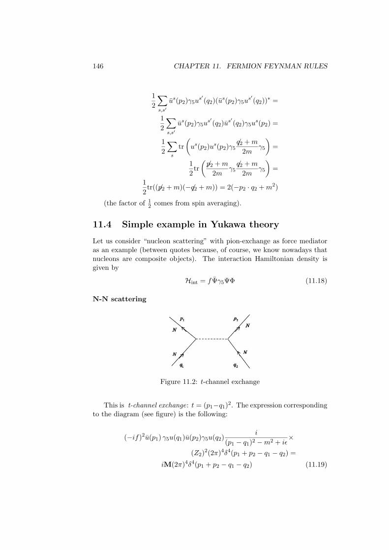
146 CHAPTER 11. FERMION FEYNMAN RULES
12
∑s,s′
us(p2)γ5us′(q2)(us(p2)γ5u
s′(q2))∗ =
12
∑s,s′
us(p2)γ5us′(q2)us
′(q2)γ5u
s(p2) =
12
∑s
tr(us(p2)us(p2)γ5
6q2 +m
2mγ5
)=
12tr(6p2 +m
2mγ56q2 +m
2mγ5
)=
12tr(( 6p2 +m)(−6q2 +m)) = 2(−p2 · q2 +m2)
(the factor of 12 comes from spin averaging).
11.4 Simple example in Yukawa theory
Let us consider “nucleon scattering” with pion-exchange as force mediatoras an example (between quotes because, of course, we know nowadays thatnucleons are composite objects). The interaction Hamiltonian density isgiven by
Hint = fΨγ5ΨΦ (11.18)
N-N scattering
Figure 11.2: t-channel exchange
This is t-channel exchange: t = (p1−q1)2. The expression correspondingto the diagram (see figure) is the following:
(−if)2u(p1) γ5u(q1)u(p2)γ5u(q2)i
(p1 − q1)2 −m2 + iε×
(Z2)2(2π)4δ4(p1 + p2 − q1 − q2) =
iM(2π)4δ4(p1 + p2 − q1 − q2) (11.19)

11.4. SIMPLE EXAMPLE IN YUKAWA THEORY 147
There is a second diagram for N-N scattering, where the two outgoing linesare exchanged. According to the above recipe, this will give a minus sign;this can also be derived from a careful evaluation of the LSZ-formula.
Figure 11.3: u-channel exchange
The Z-factors are not of great interest here; they will become importantin the discussion of renormalization. The propagator 1/(p1 − q1)2 −m2 inthe t-channel gives, after Fourier transformation of the evaluated iM (theamplitude), the Yukawa potential, which is well known in nuclear physics.
N-N scattering
Figure 11.4: s-channel exchange
This is s-channel exchange: s = (q1 + p2)2. The diagram is the same,except for the exchange of p1 and q2. The corresponding expression is
(−if)2v(−p1) γ5u(q1)u(p2)γ5v(−q2)i
(p1 − q1)2 +m2 + iε×
(Z2)2(2π)4δ4(p1 + p2 − q1 − q2) (11.20)

148 CHAPTER 11. FERMION FEYNMAN RULES
Another diagram that represents this type of scattering is shown below,and has the following expression:
(−if)2u(p1)γ5u(q1)v(−p2)γ5v(−q2)i
(p1 − q1)2 +m2 + iε× . . . (11.21)
Notes
• In Peskin & Schroder, in the spirit of time-ordered perturbation theory,outer one-particle states are directly contracted with vertex-fields:
〈p1q2| Ψγ5ΨΨγ5Ψ |q1p2〉
The required permutations give rise to extra minus signs, which includesigns related to the fermion statistics of the outer states. Altogether,this gives the u, u, v and v as above.
• A closed fermion loop gives a minus sign, as mentioned above:
〈0|T(Ψ(x1)Ψ(x1)Ψ(x2)Ψ(x2)) |0〉 →−Ψ(x1)Ψ(x2)Ψ(x2)Ψ(x1)
Figure 11.5: Closed fermion loop
Feynman approach vs. time-ordered perturbation theory
In the Feynman approach the propagators are off-shell and one has 4-momentum conservation at the vertices.
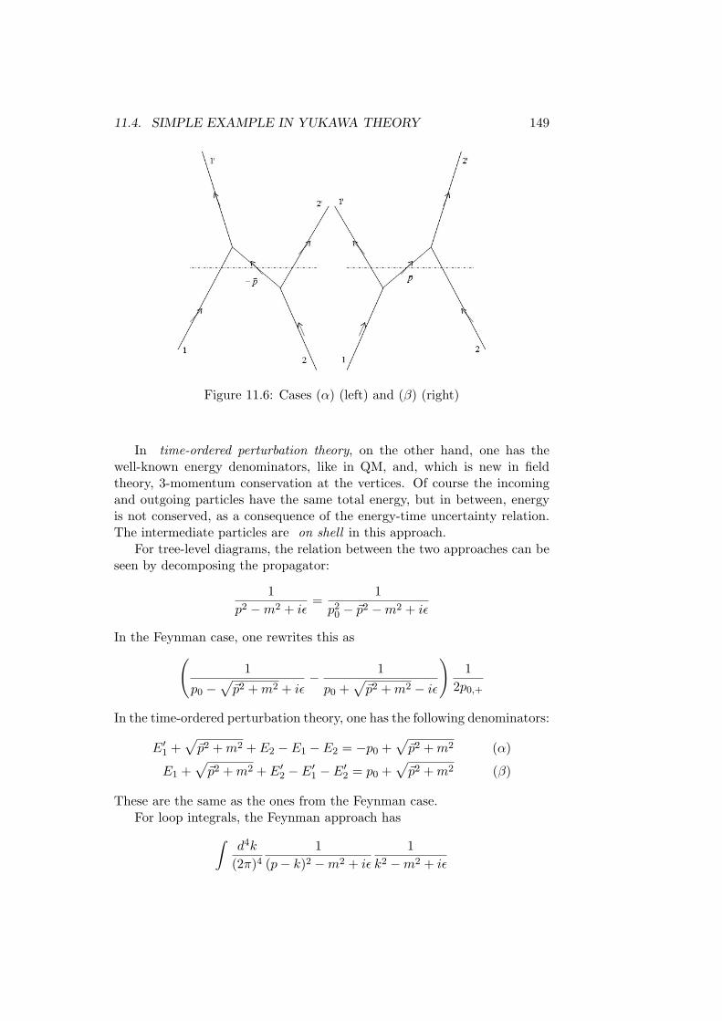
11.4. SIMPLE EXAMPLE IN YUKAWA THEORY 149
Figure 11.6: Cases (α) (left) and (β) (right)
In time-ordered perturbation theory, on the other hand, one has thewell-known energy denominators, like in QM, and, which is new in fieldtheory, 3-momentum conservation at the vertices. Of course the incomingand outgoing particles have the same total energy, but in between, energyis not conserved, as a consequence of the energy-time uncertainty relation.The intermediate particles are on shell in this approach.
For tree-level diagrams, the relation between the two approaches can beseen by decomposing the propagator:
1p2 −m2 + iε
=1
p20 − ~p2 −m2 + iε
In the Feynman case, one rewrites this as(1
p0 −√~p2 +m2 + iε
− 1
p0 +√~p2 +m2 − iε
)1
2p0,+
In the time-ordered perturbation theory, one has the following denominators:
E′1 +√~p2 +m2 + E2 − E1 − E2 = −p0 +
√~p2 +m2 (α)
E1 +√~p2 +m2 + E′2 − E′1 − E′2 = p0 +
√~p2 +m2 (β)
These are the same as the ones from the Feynman case.For loop integrals, the Feynman approach has∫
d4k
(2π)41
(p− k)2 −m2 + iε
1k2 −m2 + iε

150 CHAPTER 11. FERMION FEYNMAN RULES
Time-ordered perturbation theory has∫d3k
1energy denominators
Here, the connection between the two approaches can be seen by doingthe dk0-integration using Cauchy’s theorem (the residue theorem), closingthe integration contour in one of the two halfplanes. One gets poles in k0,yielding the required energy denominator in the residue.
For example, in Φ3 scalar theory, for the graph in figure 11.6, one has
(−iλ)2∫
d4k
(2π)4i
k2 −m2 + iε
i
(p− k)2 −m2 + iε=
(−iλ)2∫
d4k
(2π)4
(1
k0 −√~k2 +m2 + iε
− 1
k0 +√~k2 +m2 − iε
)1
2k0,+× 1
(p0 − k0)−√
(~p− ~k)2 +m2 + iε− 1
(p0 − k0) +√
(~p− ~k)2 +m2 − iε
×1
2(p0 − k0)+
(This is a rough calculation, just to see the principle; we will not worry aboutinfinities here.) Closing the integration contour in the lower half plane andapplying the residue theorem gives
(iλ)2∫
d3k
(2π)4(−2πi)
12k0,+
12(p0 − k0)+
× 1
p0 −√~k +m2 −
√(~p− ~k)2 +m2
− 1
p0 +√~k +m2 +
√(~p− ~k)2 +m2
− 1
p0 −√~k +m2 +
√(~p− ~k)2 +m2
+1
p0 −√~k +m2 +
√(~p− ~k)2 +m2
Chapter 12
Quantum mechanicalinterpretation of the Diracequation
In this chapter, we will investigate the relation between the Dirac andSchrodinger equations in the non-relativistic limit, and study the Foldy-Wouthousen transformation.
12.1 Interpretation as Schrodinger equation
If one reinserts the β- and α-matrices used in deriving the Dirac equation(chapter 10), it takes the form
i∂tΨ(~x, t) =
(mβ +
~α · ~∇i
)︸ ︷︷ ︸
H
Ψ(~x, t) (12.1)
This looks very similar to the Schrodinger equation. It is Hermitean (β = β†
and ~α = ~α†) and H2 = m2 + ~p2. Defining ρ by
ρ(~x, t) = Ψ†Ψ = Ψγ0Ψ (12.2)
one obtains a continuity equation:
∂µ(ΨγµΨ) = (∂µΨ)γµΨ + Ψ∂µγµΨ = 0 (12.3)
where in the last step, we have used the Dirac equation: (iγµ∂µ−m)Ψ = 0,and its barred couterpart ∂µΨ(−iγµ)− Ψm = 0,
All in all, it looks like we could try to interpret the Dirac equation like aSchrodinger equation without “second quantization”. However, there is oneimportant difference: the Dirac equation has negative energy solutions. The
151

152 CHAPTER 12. QM INTERPRETATION OF DIRAC EQUATION
Hamiltonian above is not bounded from below in any way; we would haveto put this in artifically, since the Schrodinger equation has only positiveenergy solutions. This means we would assume
Ψ(x) =∫
d3p
2p0(2π)3∑s
as(p)us(p)e−ipx (12.4)
without the b-term we had in chapter 10. If we do this,∫d3xΨ†Ψ =
∫d3xΨγ0Ψ =
∫d3pΨ†(p)Ψ(p) (12.5)
has a probability interpretation. Note that
Ψ(p) =∑s
as(p)us(p)((2π)32p0)1/2
(12.6)
We want to be able to calculate expectation values
〈Ψ|A |Ψ〉 =∫d3xΨ†AΨ
like in QM. Assuming an ~X which acts on Ψ(x) like a multiplication by ~x,we can calculate, by Ehrenfest’s theorem,
d
dt
∫d3xΨ† ~XΨ = i
∫d3xΨ†[H, ~X]Ψ
Writing out the commutator in the integrand, we have
[−i~α · ~∇+ βm, ~X] = − i~α sod
dt〈~x〉 = 〈~α〉 (12.7)
i.e., α acts like a velocity. Since
[H, ~α] 6= 0
we know that this “velocity” changes. Its expectation value, assuming bothpositive and negative energy solutions, is
〈~α〉 =∫
d3p
(2π)32p0
~p
p0
∑s
|as|2 + |bs|2
+ (12.8)
∫d3p
(2π)32p0
12p0
2∑s,s′=1
as
′∗(−~p)bs′∗(~p)us′(~p)~αvs(~p)e2pi0x0+
bs′(−~p)as(~p)vs′(~p)~αus(−~p)e−2ip0x0

12.1. INTERPRETATION AS SCHRODINGER EQUATION 153
The first term reproduces the usual group velocity ~p/p0; the last term mixesthe positive and negative energy solutions (more properly said, it mixes thea- and b-modes; the energies p0 are always positive). If ~α is a velocity, andα2i = 1 as we have seen before, this must be interpreted as a zitterbewegung: a
movement with the velocity of light and changing direction. This movementarises since operators corresponding to interactions, e.g. ~X, lead out ofthe space of positive frequencies. This leads to the question why radiativetransitions from positive to negative energies are impossible.
Figure 12.1: The Dirac sea, with occupied negative energy states
Here, we will introduce the concept of the Dirac sea (fig. 12.11). Diracpostulated that all states with negative energy are occupied in the groundstate of the system. In this case, the Pauli principle forbids transition tothese states, which together form the Dirac sea. In this view, the excitationof an electron with negative energy, Ee < −me, due to electromagnetic radi-ation with Eγ > 2me results in an electron with positive energy and a hole,i.e. an unoccupied negative energy level. This hole behaves like a particlewith opposite charge, i.e. a positron, and therefore, the above process isjust that of pair creation. Pair annihilation occurs when an electron emitselectromagnetic radiation and jumps down into an existing hole:
e+ + e− → 2γ (12.9)
The fact that there are two photons being produced is a consequence ofcertain conservation laws we will return to at a later time. The relationbetween positive and negative energy solutions is given by a kind of chargeconjugation. Be careful, however: in this picture, there are no anticommut-ing Fourier coefficients. It may at times pop up in old literature or in solidstate physics, but we will use the “second quantized picture”.
1Taken from http://www.phys.ualberta.ca/ gingrich/phys512/latex2html/node63.html,accessed 30-09-2007.
154 CHAPTER 12. QM INTERPRETATION OF DIRAC EQUATION
12.2 Non-relativistic limit
12.2.1 Pauli equation
In the non-relativistic limit, the Dirac-Pauli choice of γ-matrices is conve-nient. A short reminder:
Dγ0 = β =(
1 00 −1
)Dγi = βαi =
(0 σi
−σi 0
)Dusp = Susp
W =1
(p0 +m)1/2
((p0 +m)χs
~σ · ~pχs)
(12.10)
Note that this u is a factorm1/2 smaller than the last time we saw it (chapter10); this is done to ensure that u†u = 1, to preserve the analogy to QM.
In the non-relativistic limit,
p0 = m+12~p2
2m+ . . . for |~p| m (12.11)
In this limit, the upper components of u are much bigger than the lowerones. This distinction between big and small components extends to thecovariant quantities:
ΨΨ = Ψ†γ0Ψ and Ψγ0Ψ = Ψ†=1︷ ︸︸ ︷
(γ0)2 Ψ are big
Ψγ5Ψ = Ψ†γ0γ5Ψ and ΨγiΨ = Ψ†γ0γiΨ are small
Ψσ0iΨ = Ψ†=1︷︸︸︷γ0γ0 γiΨ is small
ΨσikΨ = Ψ†γ0γiγkΨ is big
As mentioned before, we write the Dirac equation as
i∂tΨ(~x, t) =
(mβ +
~α · ~∇i
)Ψ(~x, t)
We will call the “Hamiltonian” HD:(mβ +
~α · ~∇i
)=
(m ~σ · ~∇/i
~σ · ~∇/i −m
)= HD (12.12)
Introducing electromagnetic interaction, we replace ∂µ by Dµ:
∂µ → ∂µ + ieAµ = Dµ
With the ansatz
Ψ = e−imx0
(ϕ1
ϕ2
)(12.13)

12.2. NON-RELATIVISTIC LIMIT 155
we obtain two coupled equations:
i∂0ϕ1 = −i~σ · (~∇+ ie ~A)ϕ2 − eφϕ1 (12.14)
i∂0ϕ2 = −i~σ · (~∇+ ie ~A)ϕ1 − eφϕ2 − 2mϕ2
We want stationary solutions with positive energy E = E − m m andϕ ≈ e−iEx0
. This condition implies
|i∂0ϕ2| 2mϕ2 and (12.15)|eφ| m (weak potential) (12.16)
This gives for the small components ϕ2:
ϕ2 ≈ −i~σ ·(~∇+ ie ~A)
2mϕ1 (12.17)
Inserting this into the equation for ϕ1 gives
i∂0ϕ1 ≈
[−~σ(~∇+ ie ~A)~σ · (~∇+ ie ~A)
2m− eφ
]ϕ1
For the vector product between the brackets, we have the following identity:
~σ · ~a~σ~b = ~a ·~b+ i~σ · (~a×~b)
(Exercise: check this.) Plugging this in gives
i∂0ϕ1 ≈
[−(~∇+ ie ~A)2
2m+
e
2m~σ · ~B − eφ
]ϕ1
with
~A =~B × ~r
2(12.18)
and constant ~B. This is the coordinate gauge, also known as the Fock-Schwinger gauge. In this simple case, writing out the square between thebrackets and rearranging terms leads us to the Pauli-equation:
i∂0ϕ1 ≈
[−~∇2
2m+
e
2m
(~L+ 2
~σ
2
)· ~B − eφ
]ϕ1 (12.19)
The factor 2 in front of ~σ/2 should actually be g, the magnetic dipole mo-ment. In the Pauli equation, which therefore is an approximation, it isassumed to be 2.

156 CHAPTER 12. QM INTERPRETATION OF DIRAC EQUATION
Remark
The Fock-Schwinger gauge can also be formulated as follows:
xµAµ(x) = 0
Aµ(x) =∫ 1
0dη ηxνFνµ(ηx)
12.2.2 Foldy-Wouthousen transformation
It would be useful to diagonalize HD, in order to have the positive energysolution only in the upper components. This can be done by the Foldy-Wouthousen transformation:
H′FW = UHDU† (12.20)
Free Dirac equation
For the free Dirac equation, U is given by
U =(
p0
2(p0 +m)
)1/2 p0 +m− ~γ · ~pp0
(12.21)
Note that with γ0† = γ0 and ~γ† = −~γ, this means that U†U = 1. One canalso rewrite the numerator of the second fraction as −(γp−m) + γ0p0 + p0;Bjorken & Drell, and Itzykson & Zuber use yet another notation:
U = eiS with S = −i~γ ~p|~p|θ(p) (12.22)
and tan(2θ(p)) =|~p|m
The action of U on a spinor u is as follows:
Uus(p) =(
p0
2(p0 +m)
)1/2
(1 + γ0)us(p) (12.23)
Here, we have used the Dirac equation to get rid of the term with (γp−m).The factor (1 + γ0) selects the upper components, like (1 + γ5) in the Weylrepresentation (see chapter 10). The Hamiltonian itself, finally, takes theform
H′FW = UHU† =p0
2(p0 +m)1p20
(−~γ · ~p+m+ p0)(−γ0~γ · ~p+mγ0)×
(12.24)
(~γ · ~p+m+ p0) = γ0p0 = γ0(m2 + ~p2)1/2
Note that γ0 is diagonal in the Dirac-Pauli basis, so this Hamiltonian isdiagonal as well, which was the original aim of the transformation.

12.2. NON-RELATIVISTIC LIMIT 157
Remark
The action of ~XFW in x-space should be multiplication with ~x. This impliesthat it must be i~∇p; hence,
~XD = U† ~XFWU
must be given by
~XD = i~∇p −i~γ
2p0+ i
~γ · ~p ~pp0
+ i[~Σ× ~p]2p0(p0 +m)
with
Σl = εlikσik =i
2(γiγk − γkγi)εlik
Exercise: check this.With this ~XD, we have the following commutation relations:
[XiD, X
kD] = 0
[XiD, P
j ] = iδij N.b.: ~PD = ~PFW (12.25)
[H′FW, XFW] = iγ0 ~p
p0
The above relations imply
d
dt
⟨~XD
⟩= i⟨[HD, ~XD]
⟩= i⟨[H′FW,
~XFW]⟩
=⟨~p
p0
⟩(12.26)
in accordance with Ehrenfest’s theorem. With this ~XD, ~XDΨ(+) containsonly positive energy solutions. The above means that we can treat problemsin the Foldy-Wouthousen representation and then transform to the Diracrepresentation by means of U.
12.2.3 Foldy-Wouthousen representation in the presence ofa constant electromagnetic field
To evaluate the Dirac equation in the presence of a constant magnetic field,we will use the Foldy-Wouthousen representation in the notation mentionedin eq. (12.22). We expand the exponential:
HFW = eiSHDe−iS = HD + i[S,HD] +
i2
2![S, [S,HD]] +
i3
3![S, [S, [S,HD]]]

158 CHAPTER 12. QM INTERPRETATION OF DIRAC EQUATION
We want to evaluate the equation up to order O(m−2). Observe that S ∝m−1 and HD = βm+ eφ+ ~α~p ≈ m, since the mass is much larger than themomentum. With the above equation in mind, we can make the followingansatz:
HFW = mγ0 + h(0) +h(1)
m+ . . . (12.27)
Let us decompose S:
eiS = eiS2eiS1
into the following S1 and S2:
S1 =−i2m
~γ(~p− e ~A)
S2 =−im2
(14ie~α · ~E − γ0
6m(~α · (~p− e ~A))3
)Since [S1, S2] ∝ m−3, we don’t have to consider these terms. This gives forH(2):
H(2) =m+ eφ+1
2m
(~∇i− e ~A
)2
− e
2m~σ · ~B − e
gm28πρ+ (12.28)
e
4m2
1r
∂φ
∂r(~σ · ~L) +O(m−3) (12.29)
The sixth term represents the spin-orbit coupling, with the Thomas factor.The fifth term (the last one on the first line) is known as the Darwin term.ρ is the charge density, given by ρ = −eδ3(~x). The electron experiences apotential V (~r + δ~r) because of the zitterbewegung. Varying V and Taylorexpanding ∆V gives roughly this term:
∆V ≈ 12· 13
1m2
~∇2V =e
61m2
δ3(~x)
The Foldy-Wouthousen representation is fine for concrete non-relativisticcalculations. It will not do for fundamental questions concerning interac-tions, in particular since minimal coupling does not hold. That is, it worksonly for fundamental particles like e, µ, q, etc., but not for protons or neu-trons.
12.3 The hydrogen atom
For the hydrogen atom, we have
H =~α · ~∇i
+ βm− e2
rand Ψ =
(φ1
φ2
)(12.30)
~α =(
0 ~σ~σ 0
), β =
(1 00 −1
)and ~Σ =
(~σ 00 ~σ
)

12.3. THE HYDROGEN ATOM 159
Plugging all of this into the stationary Dirac equation gives(m− e2
r
)φ1 − i~σ · ~∇φ2 = Eφ1(
−m− e2
r
)φ2 − i~σ · ~∇φ1 = Eφ2
(12.31)
H commutes with ~J = ~x × ~P + 12~Σ, i.e. with ~J2 and J3. Letting the space
inversion operator Π act on Ψ gives
ΠΨ(~x) = βΨ(−~x)
So, Ψ = Ψj,m is characterized by j and m, with ~j = ~L+ 12~σ and formed out
of Y and χ±. Since j = l± 12 , and the l-term gives a parity factor (−1)l, we
introduce Φ(±)j,m. Equations (12.31) can be solved:
En,j =m
(1 + e4(n− (j + 12) + ((j + 1
2)2 − e4)1/2)−2)1/2(12.32)
with n ≤ j + 12 and j = 1
2 ,32 , . . . . Thus the degeneracy in l is partially
removed:
[figure]
Remarks
~J commutes with H, but in case ~L and ~S are coupled, ~L and ~Σ do notseparately commute with H. Therefore, it is preferable to consider thethese commutators in the Fouldy-Wouthousen representation,
~L′D = e−iS~LFWeiS
~Σ′D = e−iS~ΣFWeiS (12.33)
where ~LFW and ~ΣFW each separately commute with HFW = γ0p0. Hencewe can see that ~L′D and ~Σ′D also separately commute with HD.
The relation to the total angular momentum is given by
~L′D +12~Σ′D = ~LD +
12~LD = ~J (12.34)
~Σ′D = Σ− iγ0(~α× ~p)p0
− ~p× (~Σ× ~p)p0(p0 +m)
The helicity operator, ~Σ′D · ~p!= ~Σ · ~p commutes with HD. Normalizing it by
division by |~p|, we have (~Σ · ~p|~p|
)2
= 1

160 CHAPTER 12. QM INTERPRETATION OF DIRAC EQUATION
i.e., ~Σ · ~p/|~p| has eigenvalues ±1 with eigenvectors χ±.There also exists a split between the 2S 1
2and 2P 1
2levels; this is the
so-called Lamb shift, which one can try to explain by the zitterbewegung.We do not take this approach, but instead treat it in the context of 1-loopperturbation theory; see later.