quantum logic gates in iodine vapor using time–frequency

Molecular Physics, Vol. 104, No. 8, 20 April 2006, 1249–1266

Quantum logic gates in iodine vapor using time–frequency

resolved coherent anti-Stokes Raman scattering:a theoretical study

DAVID R. GLENN*yx, DANIEL A. LIDARy and V. ARA APKARIANz

yChemical Physics Theory Group, Chemistry Department, University of Toronto,80 St. George St., Toronto, Ontario M5S 3H6, Canada

zChemistry Department, University of California, 516 Rowland Hall,Irvine, CA 92697-2025, USA

(Received 14 July 2005; in final form 5 October 2005)

We present a numerical investigation of the implementation of quantum logic gates through

time–frequency resolved coherent anti-Stokes Raman scattering (TFRCARS) in iodine

vapour. A specific scheme is given whereby two qubits are encoded in the tensor product space

of vibrational and rotational molecular eigenstates. Single-qubit and controlled-logic gates

are applied to test the viability of this encoding scheme. Possible experimental constraints

are investigated, including the necessary precision in the timing of successive CARS pulses and

the minimum resolution of spectral components within a given pulse. It is found that these

requirements can be satisfied by current technology. The two-qubit Grover search is

performed to demonstrate the implementation of a sequence of quantum operations. The

results of our simulations suggest that TFRCARS is a promising experimental system

for simple quantum information processing applications.

Keywords: Quantum logic gates; Iodine vapour; Time–frequency resolved coherent anti-StokesRaman scattering

1. Introduction

Interest in the study of quantum information and

quantum computation has increased tremendously in

the past decade. The origin of the field is commonly

attributed to Feynman [1], who proposed that one

quantum mechanical system could be used to efficiently

simulate others. Benioff [2] and Deutsch [3] also made

important early contributions to our understanding

of the relationship between classical and quantum

computation. The recent surge in activity is due in

large part to the development of important quantum

algorithms by Shor [4] and Grover [5]. The former

provides a method for factoring large numbers into

primes that scales polynomially in the number of digits.

The latter allows a search through a list of N elements

to be conducted in O(N1/2) steps, which is provablyfaster than the best possible classical algorithm.

Numerous candidate systems have been suggested forthe physical implementation of a quantum computer.The problem is a challenging one, due to the intrinsic

trade-off between long decoherence times and the easewith which quantum states may be prepared andmeasured. The proposals that have been experimentallydemonstrated to date are liquid-state NMR [6], cavityQED [7], cold trapped ions [8] superconducting tunnel

junctions [9], and quantum dots [10]. A number of recentstudies have focussed on the possibility of encodingquantum bits into molecular states that can be manipu-lated through nonlinear optical interactions [11–14].

The present investigation explores the use oftime–frequency resolved coherent anti-Stokes Ramanscattering (TFRCARS) to create and manipulate

ro-vibronic coherences in molecular iodine vapour.It has been shown that the structure of time-resolvedCARS gives access to the operations necessary foruniversal quantum computation, namely arbitrary

*Corresponding author. Email: [email protected]

xPresent address: Department of Physics, Yale University, Sloane

Physics Lab, 217 Prospect Street, New Haven, Connecticut

06511-8499, USA.

Molecular PhysicsISSN 0026–8976 print/ISSN 1362–3028 online � 2006 Taylor & Francis

http://www.tandf.co.uk/journalsDOI: 10.1080/00268970500525713

single-qubit rotations and a two-qubit controlled-NOTgate [11]. Previous calculations have demonstratedhow a coherent computation can be carried out withTFRCARS on the vibrational states of I2 [12]. Thisresearch extends those results by developing a numer-ical simulation of the system in the full ro-vibronicHilbert space, consisting of the tensor products ofBorn–Oppenheimer separated electronic, vibrational,and rotational states.This paper is structured as follows. In section 2, we

provide a brief overview of the experimental CARSsystem, and the theoretical methodology of double-sided Feynman diagrams used to describe this system.In section 3 we describe our simulations and schemefor encoding quantum information into electronic andro-vibrational states. In section 4 we present our resultson a simple quantum algorithm implemented usingTFR-CARS in iodine. We conclude in section 5.

2. The system

Here, we give a physical description of the CARSsystem. Relevant references include [11, 15, 16], as wellas Mukamel’s text on nonlinear optics [17], severalgeneral texts on molecular spectroscopy [18–20], and anumber of other papers on modeling CARS systems[21–23].

2.1. The experiment

The numerical simulation we present later is modeledafter ongoing experiments being carried out in theApkarian group. A schematic representation of theapparatus, taken directly from one of their recent

papers [15], is shown in figure 1. The I2 vapourresides in a quartz cell at 0.3 Torr, heated to 50�C.Three phase-locked, linearly polarized optical pulsesinteract successively with the molecules over a timeinterval on the order of tens to hundreds of picoseconds.These pulses establish and manipulate the quantumcoherences used to perform the computation. In thestandard CARS nomenclature, the pulses are namedaccording to the order in which they interact with thesystem: The first is labelled P, for ‘pump’; the second S,for ‘Stokes’, because it is traditionally tuned to thered of the first pulse; and the third P0, either for‘probe’, or because it is often the same colour as thefirst pulse. These pulses are initially generated by aTi:sapphire laser, with its output compressed to 70 fsand 700 mJ/pulse by chirped pulse amplification. This issplit to two optical parametric amplifiers (OPA), theoutputs of which are up-converted by sum generationto be tuneable in the near infrared, 480–2000 nm. TheP and P0 pulses are obtained by splitting the outputof one OPA, while the second OPA generates theS pulse. The spectrum of each pulse is precisely shapedusing a spatial light modulator before it interacts withthe sample. All pulses are chosen to be resonant withthe dipole allowed X(1

P0gþ)$B(3

Q0uþ) electronic

transition.The part of the macroscopic polarization due to

the subset of iodine molecules that interact exactlyonce with each pulse generates the experimental signal.This is the so-called AS, or ‘anti-Stokes’ radiation.It is separated from the other scattered light byspatially filtering along the direction of the anti-Stokeswave-vector, kAS¼kP� kSþ kP0, which correspondsto the CARS energy conservation condition !AS¼

!P�!Sþ!P0. The anti-Stokes signal is precisely trun-cated in time by passing it through a pair of cross-polarized prisms surrounding a Kerr cell. Rotationis induced in the cell by a small fraction of the original800 nm fundamental Ti:sapphire output, which hasbeen polarized at 45� to the AS radiation and timedwith a delay line. The resulting AS pulse is dispersedin a monochromator and directed onto a CCD arrayfor detection.

2.2. Calculating the molecular polarization

Evolution of molecular states under the influenceof the applied pulses is calculated in the time domain,using the formalism of time-dependent perturbationtheory. The interaction Hamiltonian is described semi-classically and in the dipole approximation,

HIðtÞ ¼ �� EðtÞ: ð1ÞFigure 1. Experiment schematic—from [13].

1250 D. R. Glenn et al.

For the perturbative approach to be valid, the field must

be weak: mE0�� h, where E0 is the average amplitude

of the pulse and � its duration. This requirement is

satisfied in the experiment.The molecular states are written in the interaction

picture, where the usual procedure of iterative integra-

tion leads to the following time evolution operator:

Uðt,t0Þ ¼ U0ðt,t0Þ þX1n¼1

�i

�h

� �n Ztt0

d�n

Z�nt0

d�n�1 � � �

Z�2t0

d�1

ðU0ðt,�nÞHIð�nÞU0ð�n,�n�1Þ

HIð�n�1Þ � � �U0ð�2,�1ÞHIð�1ÞU0ð�1,t0ÞÞ: ð2Þ

The operator U0 describes evolution under the free

molecular Hamiltonian H0. Since we are concerned only

with states which undergo exactly three interactions

with the electromagnetic field, the sum can be truncated

at n¼ 3.The expression for the matrix elements of the

molecular polarization, at third order, is given by

Pð3ÞðtÞ ¼ ð3ÞðtÞj�j ð0ÞðtÞ� �

þ ð2ÞðtÞj�j ð1ÞðtÞ� �

þ c:c: ð3Þ

Here, j (j)(t)i is obtained by applying the jth term in

the sum from equation (2) to the initial state j (t0)i.The expression for P(3) is summed over all molecules

to obtain the macroscopic polarization, which acts as

a source in Maxwell’s equations. The observed field,

EAS, is therefore directly proportional to P(3).In the simplest case, the expression in equation (3)

contains four terms. When the dipole Hamiltonian in (1)

is substituted into (2), indices must be added to the E

field to distinguish the three pulses: EP, ES, EP0. Because

of the spatial filtering in the experiment, it is guaranteed

that the system will interact with each pulse exactly

once. However, if the pulses overlap temporally, multi-

ple time orderings may be possible in the evaluation

of (2). In principle, all permutations of the three pulse

indices must be calculated, increasing the total number

of terms in (3) to 24. Practically, most of these terms

will be almost zero except where, for instance, EP(t) and

ES(t) both have non-negligible amplitudes for the

same value of t.It is common to use time circuit diagrams to depict

each of the terms of equation (3). Examples of such

diagrams are illustrated in figure 2. The horizontal

direction represents time, while the vertical describes the

energy of the state. In the Born–Oppenheimer approx-

imation, states shown above the dotted line are

ro-vibrational levels in the excited (B) electronic state,

while those below the line are in the ground (X)

electronic state. Each diagram illustrates the interac-

tions undergone by both the bra j (j)i and the ket

h (j�3)j. Figure 2(b), for instance, describes the following

sequence. (i) The ket interacts with the P pulse at t1and is excited from the X to the B electronic state.

(ii) The bra interacts successively with the S pulse at t2and the P0 pulse at t3, remaining on the B surface during

the interval between those pulses. (iii) At some later time

t the coherence between the bra and ket spontaneously

collapses, and a photon is emitted which will contribute

to the AS radiation. This contribution adds to the term

denoted h (2)(t)jmj (1)(t)i in equation (3).Of the three diagrams displayed, only the one in

figure 2(a) typically makes a significant contribution to

the macroscopic polarization. The diagram in figure 2(b)

is suppressed because it begins from an excited initial

level, which will have a smaller amplitude than the

vibrational ground state in a thermal distribution.

The diagram in figure 2(c) will not contribute signifi-

cantly because the transition excited by the P0 pulse

is not resonant. The full integral expression for the

contribution from figure 2(a) is as follows [23]:

Pð0,3ÞAS ðtÞ ¼

k

�h3

Zt�1

dt3

Zt3�1

dt2

Zt2�1

dt1

eði=�hÞHXt�

j�j eð�i=�hÞHBðt�t3Þ� � EP0 ðt3Þ eð�i=�hÞHXðt3�t2Þ�

�E�Sðt2Þ e

ð�i=�hÞHBðt2�t1Þ� � EPðt1Þ eð�i=�hÞHXt1

�þ c:c: ð4Þ

(a) (b) (c)

Figure 2. Sample time-circuit diagrams.

Quantum logic gates in iodine vapor using time–frequency 1251

Evaluation of the dipole matrix elements is performedin the Franck–Condon limit, so that m in equation (4)may effectively be replaced by the product of the spatialoverlap of the initial and final vibrational wavefunctionsand a constant associated with the X and B electronicstates. This must be multiplied by a rotational matrixelement [20] to account for all possible magneticquantum numbers when the interaction with a linearlypolarized field changes the total angular momentumof the state by �1. Thus, the complete expression forthe dipole matrix element between Born–Oppenheimerseparated states of the form �e,v,J is given by

�e,v,Jj�j�e0,v0,J�1

� �¼ �e,e0 �ðrÞj�

0ðrÞ� �

Dj, j�1, ð5Þ

where the rotational matrix element is the sum overClebsch–Gordan coefficients

Dj, j�1 ¼Xj

m¼�j

j,m; 1,0j j� 1,m� �

: ð6Þ

It can be shown [23] that the time domain representationof the contribution to the polarization in equation (4)is equivalent to a more commonly encountered fre-quency domain expression involving the so-calledhyperpolarizability tensor, �:

Pð3Þ� ð!z0Þ¼��E

�ð!1ÞE�ð!2ÞE

�ð!3Þð!1�!2þ!3�!0Þ:

ð7Þ

Furthermore, Mukamel shows [17] that expression (4)is equivalent, for a pure initial state, to his morecomplicated general expression involving density oper-ators evolving in Liouville space. Although the initialstate of the physical system is actually a thermaldistribution, it turns out that this simplification is stillvalid for our purposes. The reason is that, for a pumppulse with sufficient spectral selectivity, only onestate in the initial thermal distribution actually con-tributes to the evolving coherence. This is demonstratednumerically in section 4.3.It is important to note that equation (4) represents the

contribution of a single molecule to the bulk polariza-tion. A macroscopic ensemble of these moleculesproduces the anti-Stokes radiation, where each sponta-neous emission event is effectively a measurement of anindependent single-particle wavefunction. Observationof the AS pulse in the frequency domain is thereforeequivalent to complete tomography of the segmentof the molecular density matrix that describes thethird-order coherence. For quantum information pro-cessing applications, the state of the qubits is encoded

in the evolving coherence. A single pulse sequenceperforms the same quantum computation on manymolecules in parallel, and the complex amplitudes of thefinal qubit states may therefore be read directly fromthe anti-Stokes radiation.

2.3. Useful pictures: vibrational wavepacketsand interferometer diagrams

Several intuitive pictures have been used to describethe evolving molecular coherence under the action ofthe CARS pulses. The simplest of these employs thelanguage of vibrational wavepackets in the positionrepresentation, oscillating on an anharmonic potential.Figure 3 gives a diagrammatic portrayal of this picture,for the large amplitude path corresponding to equation(4) and figure 2(a). At time t1, the P pulse interacts withthe molecules in the electronic ground state (0) toproduce a vibrational wavepacket (1) on the excitedelectronic potential. The shape of this packet is deter-mined by the relevant Franck–Condon factors, andone often speaks of the Franck–Condon ‘window’ ofbond-lengths at which a vertical transition may occur.This window is located near the turning points of thepotential, where a classically oscillating object wouldspend most of its time. The excited packet evolves on theB electronic surface until the arrival of the S pulse at t2.The part of the packet overlapping with the Stokeswindow then returns to the ground electronic state (2).(Note that the position of the window is influencedto some extent by the mean frequency of the pulse,which determines the locations of the turning points.This can, of course, be understood more precisely bydecomposing the wavepackets into eigenstates of thevibrational potentials). The packet now continues toevolve until t3, when the P0 pulse again transfers theportion overlapping its Franck–Condon window to the

Figure 3. Vibrational wavepacket picture.


B electronic surface (3). The system is now in a third-

order coherence, where all pulses have acted on the

ket wavefunction and none on the bra. The excited

wavepacket oscillates on the excited potential, radiating

spontaneously every time it reaches the AS window at

the inner turning point, corresponding to the energy

conservation condition !AS¼!P�!Sþ!P0. The macro-

scopic coherence persists until all molecules have emitted

photons, or (more realistically) until it is destroyed

by collisions.The wavepacket picture assumes pulses of sufficient

spectral width to transfer large superpositions of vibra-

tional eigenstates. This situation is less than optimal

for quantum information processing in the TFRCARS

system, because it implies interference between the

information-encoding states and those outside the com-

putational space. Furthermore, wave packets become

difficult to visualize when spherical harmonics are

introduced to describe the rotational degree of freedom.

An alternative description is therefore required. Figure 4

shows one possibility, where paths through Hilbert

space involving particular pairs of vibrational states

(or rotational states) are considered separately. Such

diagrams draw attention to the phases acquired by

individual eigenstates, with each pair of doubly inter-

secting paths effectively equivalent to a Mach–Zender

interferometer in optics.

The interferometer diagram for the vibrational qubitis illustrated in figure 4(a). Solid diagonal arrowsrepresent interactions with the electromagnetic field;open horizontal ones indicate evolution under the baremolecular Hamiltonian. In general, an arbitrary phasemay be associated with each arrow, and an arbitraryamplitude with each one describing a field interaction.(In fact, in the limit of perfectly selective pulses, thephase acquired during free evolution is fixed; this willbe discussed further in section 4.1). The vibrationalquantum numbers of the states used to encode the |0ivand |1iv parts of the qubit at each step may be chosenfreely by selecting appropriate frequencies for thespectral components of the pulses. Interference occurswhenever two non-zero diagonal arrows terminate inthe same state. The total action on the vibrationalqubit is therefore equivalent to two consecutive pairs ofinterlocking Mach–Zender interferometers, with eachmirror capable of transmitting and reflecting the inputsignal at arbitrary phases, as well as freely attenuatingor amplifying it.

Figure 4(b) shows the analogous diagram for therotational qubit. Note that, in this case, dipole selectionrules limit the allowed transitions, so that a morecomplex interferometer is required to effect the trans-formations desired for quantum information processing.Once again, the diagonal arrows represent pulse inter-actions, with which an arbitrary complex amplitude maybe associated.

In the v� J tensor product representation, eachpath of the vibrational interferometer should havethe components of the rotational interferometer for therelevant time interval superimposed on it. It can beshown that the interferometers depicted contain suffi-cient degrees of freedom to implement arbitrary SU(2)transformations on each of the qubits, given thatthe spectral components of the pulses are able toresolve rotational transitions independently. Deletingthe appropriate arrows in the ‘tensor-product of inter-ferometers’ may produce controlled operations, as longas the pulses are chosen so that each arrow correspondsto an independent spectral component. An importantfeature to notice in the interferometer diagrams is thefreedom they allow in choosing the amplitude associatedwith each diagonal arrow. This underscores the fact thatthe transformations performed in the space of qubitsare fundamentally non-unitary: doubling the amplitudeof all spectral components of a given pulse will causea corresponding doubling in the total amplitude of theoutput state. Normalization of the qubits must there-fore be treated with some care. Finally, note thatthe diagrams of figure 4 illustrate the case where allthree pulse-operators (i.e. m�Ei) act on either the braor the ket, as in figures 2(a) and 3. To represent other

(a)

(b)

Figure 4. (a) Vibrational-state interferometer. (b) Rotational-state interferometer.


Liouville paths, one could replace the appropriate pulses

with zero-phase horizontal arrows.

3. Quantum logic gates using TFRCARS

We now describe how quantum information can be

manipulated and processed using TFRCARS.

3.1. Encoding qubits and quantum gates

At the highest level of abstraction, the quantum com-

putation consists of collection of three-pulse sequences,

each of which represents a single quantum gate.

Following the paradigm described in [11], the P pulseprepares the initial states of the qubits in the quantum

register, the S pulse performs the desired transforma-

tion, and the P0 pulse prepares the system for readout.

This procedure is repeated for each gate, until the full

quantum algorithm has been implemented.The P pulse consists of up to four spectral compo-

nents, each of which excites a transition from some

chosen original eigenstate in the thermal ensemble to aneigenstate encoding one of the tensor-product compu-

tational basis states. The original level on the ground

electronic surface from which the computation is initi-

ated may be chosen freely; the most common choice in

our simulations has been |X, v0¼ 0, J0¼ 52i, which

has the maximum amplitude in a thermal distribution at

298K. The vibrational quantum numbers of the encod-

ing states are also arbitrary, although the rotational

levels must be related to the original eigenstateby �J¼�1. By convention the |J0þ 1i states encode

the |1iJ part of the rotational qubit, and the |J0� 1i

states the |0iJ part. Likewise, the higher vibrational level

typically encodes the |1iv part of the vibrational qubit.

The amplitude and phase of each component of the

initial state are determined by the amplitude and phase

of the corresponding P pulse component. In order to

avoid contaminating the calculation by exciting transi-tions from initial thermal eigenstates other than the

desired one (i.e. other than |X, 0, 52i), the spectral

components of the P pulse should be fairly narrow. In

practice, it seems to be sufficient to choose the width of

each component to be less than one-tenth the energy

difference between the desired transition and the one

connecting neighbouring rotational states. For instance,

if the transition to be excited is |X, v, Ji!|B, v0, Jþ1i,then the width of the pulse component, �, is chosen

to satisfy

10 �h� < ðEB,v0,Jþ1 � EX,v,JÞ � ðEB,v0,Jþ2 � EX,v,Jþ1Þ�� : ð8Þ

This typically results in a value for � on the orderof 0.16 cm�1, corresponding to a transform-limited pulse

duration of about 200 ps in the time domain. The twotransitions |v, Ji!|v0, Jþ1i and |vþ1, Ji!|v0þ1,

Jþ1i are not degenerate, primarily due to the anharmo-nicity of the vibrational potential. Note condition (8) isconsiderably more stringent than merely requiring the

spectral component not to overlap with the nearestdipole-allowed rotational state, i.e. �h�<|EX, v0, Jþ1�

EX, v0, J–1|. Adherence to (8) does not eliminate allundesired transitions, but empirically seems to keep the

number small enough that most extraneous paths areremoved by the selectivity of the S and P0 pulses.

In the most successful encoding scheme the S pulsecontains 16 spectral components, roughly correspond-

ing to the elements of the 4� 4 matrix representingthe two-qubit quantum gate. The spectral width ofeach component is chosen the same way as for the

P pulse. In this scheme the selection of the next pair ofvibrational levels is again unrestricted, although it

may be helpful to choose them such that all fourpossible transitions from the first two vibrational levelshave Franck–Condon factors of comparable magnitude.

This is not strictly necessary, because the amplitudeof each spectral component can be multiplied by a

constant to compensate for the FC factor, althoughit does help to ensure that no single component is muchstronger or weaker than the others. One might suspect

that the S pulse should also include a phase correctionto compensate for the free evolution the state has

undergone since interaction with the P pulse, but thisturns out to be unnecessary (see section 4.1). Finally,recall that the S pulse temporarily splits the rotational

qubit into three separate states, which are later recom-bined by the P0 pulse (cf. figure 4(b)). The complex

amplitudes chosen for the components that perform thissplitting are such that the three levels can be recombined

equally and in phase to produce the desired gate. Thisis illustrated in figure 5, which shows the rotationalinterferometer that will perform a unitary transforma-

tion on the rotational qubit specified by the matrix

A BC D

� �:

Thus, the initial state a0|0iJþ a1|1iJ goes to (Ca1þDa0)|

0iJþ (Aa1þBa0)|1iJ, given that the component of the Spulse connecting states |J0� 1i!|J0� 2i has relativeamplitude (D–B), the one connecting |J0� 1i!|J0i has

amplitude B, and so forth. In addition, note that eachrotational transition should be multiplied by a constant

to compensate for the rotational matrix elementof that transition. The four components of figure 5


associated with the S pulse are all repeated four times,once for each possible vibrational transition. Each setof four is multiplied by a complex constant associatedwith the matrix element connecting the two states of thevibrational qubit.The P0 pulse is the simplest of the three, consisting

of eight spectral components with widths determinedby the same criteria as for the P pulse. Apart fromcorrections for FC factors and rotational matrixelements, all components have equal amplitude.Corrections are made for FC factors and rotationalmatrix elements associated both with the transitioninduced by the P pulse, and the spontaneous emissionevents which produce the anti-Stokes signal. The pulsehas only eight components because it does not performany processing, so that transitions connecting the |0iVwith the |1iV states of the vibrational qubit areunnecessary.Readout is achieved by collecting the anti-Stokes

radiation during a fixed time window, and computing itsFourier transform. It is important to ensure that thewindow begins only after the last pulse has finishedinteracting with the system, to avoid introducingerrors in the phase data. The duration of data collectionis typically 800 ps, corresponding to roughly 219 gridpoints (where the time grid spacing is set by the durationof one half of an optical period). The time domain dataare multiplied by a sinusoid at the transition frequencybetween the lowest states on the X and B electronicmanifolds. This has the effect of shifting all thefrequency components down by about 15 000 cm�1,and greatly reduces the number of points required foran accurate transform. The final amplitudes of thequbits after the gate are read off by integrating thepower spectrum over narrow intervals (0.2 cm�1)around the expected transitions. The phases can bereliably determined from the argument of the complexfrequency-domain data, the spectrum of which looks

much as one would expect for a driven oscillator nearresonance. An example of the amplitude and phasedata for the rotational qubit is shown in figure 6. Thestate depicted has equal amplitude in both compo-nents and a relative phase of roughly zero. Hence it isapproximately | i 2�1/2(|0iJþ|1iJ).

Reading the phase data in the simulation correspondsto making a heterodyne measurement in the lab.Detection of the amplitude and phase of all peaks inthe anti-Stokes spectrum gives a complete state tomog-raphy of the qubit density matrix. Thus, a singlesequence of three pulses is sufficient to test thebehaviour of the encoded gate for a given initial state.This fact is also useful when the goal is to implementa more complex quantum operation, consisting of thesequential application of multiple gates. In that case,the procedure is to apply one gate, record the resultinganti-Stokes spectrum, and then perform the followinggate on a new thermal ensemble. The P-pulse of thesecond gate prepares an initial state in the new systemexactly equal to the output state of the first gate. Inorder to properly interpret the anti-Stokes data, a cali-bration must be performed before every gate. Thisconsists of a series of pulse sequences correspondingto Iv� IJ transformations on each of the four compu-tational basis states. The calibration provides a referencewith respect to which the phase of the AS radiationfor the gate pulse sequence may be read.

4. Results and discussion

This section describes the main numerical resultsobtained with the TFRCARS simulation. Our primaryfocus has been to elucidate the experimental constraintson the optical fields required to generate, manipulate

Figure 5. Encoding rotational state transformation.

Figure 6. Simple anti-Stokes spectrum.


and detect the coherences used for encoding quantuminformation in this system. In subsection 4.1, we inves-tigate the effect of uncertainties in the arrival timesof the Raman pulses in the time domain, as well as in thetime-gated detection scheme. Subsection 4.2 examinesrequirements on the frequency widths of each spectralcomponent of a particular pulse, and hence on theresolution of the spatial light modulator used togenerate the pulses. Finally, subsection 4.3 suggestshow a multi-step quantum-processing task might be per-formed in the TFRCARS system, using the two-qubitGrover search algorithm as an illustration.Much of the data in this section is displayed in terms

of the fidelity of the observed quantum gate, plottedagainst the simulation variable of interest. For ourpurposes, fidelity is computed as the modulus of theinner product of the observed final state of the simula-tion with the output state expected from an ideal gate,given a particular input state. Symbolically,

Fj ii ¼jh’expj fij

jj fij2

, ð9Þ

where Fj ii is the fidelity given input state | ii, and |’expiand | fi are the (properly normalized) expected outputstate vector, and the (un-normalized) observedoutput state.A better description would minimize this product over

all possible input states (see [28], p. 417). Unfortunately,performing the minimization over all inputs in twoqubits would be numerically very time-consuming.Nonetheless, we expect that the present descriptionshould provide a reasonable qualitative picture. The bestway to obtain the desired transformations is to eliminateor minimize the amplitudes of all extraneous pathsthrough the state space. Empirically, the fidelitiescorresponding to the computational basis states aloneshould give a good idea as to whether this hasbeen achieved.

4.1. Requirements for pulse delaysand time-gated detection

Among the first questions one may consider using theTFRCARS simulation is that of the requirements onthe precision in arrival times of the P, S, and P0 pulsesnecessary for implementing quantum operations withhigh fidelity. We found that, for pulses with sufficientlynarrow spectral components (i.e. satisfying equation(8)), the observed anti-Stokes spectra are insensitive tochanges in the time delays between the various pulses.Initially, this observation seems counterintuitive; in theusual picture of a two level quantum system, the relative

phase between the states will oscillate in time if no

interaction is imposed. In our perturbative formalism,

however, it turns out that each pulse interaction

effectively cancels the phase accrued during the free

evolution period following the preceding pulse. As a

simple demonstration, consider the case of two popu-

lated levels that undergo a free evolution starting at

time t¼ 0, and then interact with the applied field at t1.

Assume the pulse arriving at t1 has two spectral

components, designed to excite resonant transitions

from initial states |�1i and |�2i to the final states �01��

and �02��

respectively. The frequency of level |�ji is

denoted !j. The final state | (t)i is then given by

j ðtÞi ¼

Z t

0

dt1 e�iHfreeðt�t1Þ=�h � � ðE1ðt1Þ e

�ið!01�!1Þt1

þ E2ðt1Þ e�ið!0

2�!2Þt1 þ c:c:Þ

� e�iHfreet1=�hðj’1i þ j’2iÞ

¼

Z t

0

dt1 e�iHfreeðt�t1Þ=�h � � ðE1ðt1Þ e

�ið!01�!1Þt1

þ E2ðt1Þ e�ið!0

2�!2Þt1 þ c:c:Þ

� ðe�i!1t1 j’1i þ e�i!2t1 j’2iÞ: ð10Þ

Roughly speaking, in the limit that the components

at (!01 �!1) and (!0

2 �!2) are spectrally very narrow,

the envelopes Ej(t1) may be represented as constants.

The dipole operator acts on the state |�ji to give |�0jionly, again assuming the spectral width is narrow

enough to give only one resonant transition. The

remaining free evolution between t1 and t (leftmost

exponential under the integral sign above) can be

replaced with exp(�i!j(t� t1)) when acting on the state

|�0ji, and the integration with respect to t1 at long times

t!1 will eliminate the non-resonant cross-terms, so

that the final result is

j ðtÞi ¼ ð�1e�i!0

1tj’01i þ �2e

�i!02tj’02iÞ þ c:c:, ð11Þ

where the mj are scalar coefficients determined by eval-

uating the dipole operator for the relevant transitions.

Thus, the duration of the free evolution between 0 and t1is irrelevant.

Note, however, that if the individual spectral compo-

nents are modeled as Gaussian curves with standard

deviations �>(!2�!1), then transitions |�1i!|�02i and|�2i! |�01i will also be excited. Then the analytical result

of the integration is more complex to evaluate, but it is

intuitively clear that integration of the Gaussian

envelopes E(tj) will no longer eliminate the cross-terms,

resulting in oscillations at �(!1�!2). Thus, the phase

accumulation between pairs of states during free


evolution is erased by the subsequent pulse, but onlyif the components of that pulse are sufficiently narrow.Phase accumulation does occur after the third (i.e. P0)

pulse of the sequence, since there is no succeedinginteraction to undo it, and this has significant implica-tions for reading out the result of a quantum operationin the TFRCARS system. As can be seen, for example,from equation (11), each final state of the computationoscillates in time, without further electromagneticfield interactions to cancel the phase accumulation.The contribution to the macroscopic polarization com-puted from any pair of these states (cf. equation (B.6))will also be time dependent, and it is this that producesthe observed optical field. In real experiments, phasedata will most likely be measured with a time-gateddetection scheme, as described in section 2.1. The phase-locked gate pulse must have a temporal length of severalhundred picoseconds to resolve the spectral lines repre-senting qubits from those of background transitions.As with the input pulses durations, this figure is equal to2 divided by the frequency distance to the nearestundesired rotational transition, approximated in equa-tion (8). The gate pulse used in the simulation is actually790 ps, which is probably longer than necessary,but provides a convenient number of data points fornumerical FFT calculation.The procedure for quantum information processing in

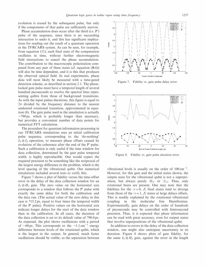
our TFRCARS simulations uses an initial calibrationpulse sequence, corresponding to the ‘do-nothing’IV� IJ operation, to measure phase offsets caused byevolution of the coherence after the end of the P0 pulse.Such a calibration is only useful if the time window fordata collection, determined by the gate pulse temporalwidth, is highly reproducible. One would expect therequired precision to be something like the reciprocal ofthe largest energy difference in the problem, which is thelevel spacing of the vibrational qubit. Our numericalsimulations included several tests to verify this.Figure 7 shows a plot of fidelity versus the time-offset

error in the delay of the data collection window for anIV�HJ gate. The zero value on the horizontal axiscorresponds to a window that follows the P0 pulse withexactly the same delay for both the calibration andthe data run. (The actual value of the zero delay in thiscase is 715.2 ps, equal to four times the temporal widthof the P0 pulse). Positive values on the horizontal axisindicate longer delays for the start of the data windowthan in the calibration. In all cases, the duration ofthe data collection is set to its default value of 790.0 ps.As expected, the plot shows oscillations with a periodof 60 ps. This corresponds to the 1.1 cm�1 energydifference between levels of the rotational qubit, whichis the largest in the output. In general, much fasteroscillations should be visible, as the separation between

vibrational levels is usually on the order of 100 cm�1.However, for this gate and the initial states shown, theoutput state for the vibrational qubit is not a superpo-sition, but always purely |0iV or |1iV. Thus, onlyrotational beats are present. One may note that thefidelities for the |v¼ 0, Ji final states tend to divergefrom those of the |v¼ 1, Ji states at large delays offsets.This is readily explained by the rotational–vibrationalcoupling in the molecular free Hamiltonian.Experimentally, gate delays on the order of hundredsof picoseconds may be controlled with femtosecondprecision. Thus, it is expected that phase informationcan be read with great accuracy, even for output statesthat involve superpositions of the vibrational qubit.

In addition to errors in the delay of the data collectionwindow, one might also anticipate uncertainty in itsduration. Figure 8 shows plots of gate fidelity, forthe same IV�HJ gate, against the error in the length

Figure 7. Fidelity vs. gate pulse delay error.

Figure 8. Fidelity vs. gate pulse duration error.


of the gate pulse. Once again the error is applied onlyto the actual gate pulse sequences, not to the calibration.The start of the gate pulse is always 715.2 ps afterthe peak of the P0 pulse, and the error is added to theend of the window. In the previous case, the shapeof the plot could be interpreted quite simply, sinceshifting the upper and lower bounds of the discreteFourier integral together is just the same as pullinga complex phase factor out of each component. Here,one integration limit is varied while the other is heldconstant, and the resulting pattern is more complex.It seems to show some periodicity at about 35 ps, but therepetition on that timescale is obviously modulated.In any case, the thing to notice is that the regionof high fidelity around zero delay is quite narrow,at less than 5 ps. Nonethless, the temporal width ofthe gate can be kept constant in experiments to within10–100 fs for a given Kerr medium, which should besufficient to avoid problems.

4.2. Pulse spectral resolution and gate fidelities

The spectral widths of the pulse components are a keyconsideration in obtaining the desired quantum gates.To the extent that spectral features are sufficientlynarrow, only the necessary transitions are excited. Nonet phase evolution then occurs for the computationalstates between pulses, and the resulting transformationcan be controlled exactly. If the widths become toolarge, however, extraneous paths begin to acquiresignificant amplitudes and can interfere with the resultof the desired computation.For this reason, a quantitative study of the influence

of component widths on gate fidelity has been under-taken. The results presented here will concentrate on therepresentative examples of HV� IJ gates, which displayfeatures characteristic of most data collected so far.Figures 9(a)–(c) show plots of fidelity versus spectral

width for HV� IJ. All four plots demonstrate fidelitiesfairly close to 1 for widths of up to about 1 cm�1.This may be significant for practical implementationsof the computing scheme, particularly in the caseof the S pulse. The reason is that, according to [24],most pulse shaping experiments are limited to ratiosof bandwidth/spectral feature size of a few hundred.Thus, resolutions of 1 cm�1 are probably attainablefor the 331 cm�1 bandwidth S pulse, while the defaultvalue of 0.2 cm�1 may not be. Limitations for theother pulses are less stringent.The high-fidelity segment of figure 9(b) is shown

on expanded axes in figure 10. For small linewidths, thecalculated fidelities are consistently between 0.999 and1.0. Because this behaviour persists to linewidthsof almost zero, such data can be used to estimate an

upper bound of about 0.001 on the numerical errorin the computed fidelities. This error likely arisesfrom integration on a finite time grid, as well asthe early truncation of some numerical constants.

(a)

(b)

(c)

Figure 9. (a) Fidelity vs. spectral width of P pulsecomponents of HV� IJ gate. (b) Fidelity vs. spectral widthof S pulse components of HV� IJ gate. (c) Fidelity vs. spectralwidth of P0 pulse components of HV� IJ gate.


Small inconsistencies in the bounds of integration for

each peak in the anti-Stokes intensity spectrum may also

contribute.Note that the normalization of final states used to

calculate fidelities in figures 9 and 10 is somewhat subtle,

due to the fact that the operations performed on the

qubits by the pulses in perturbative TFRCARS are

not unitary. (This is, of course, a result of the fact that

we are only considering the third-order coherence

at the final step of the calculation; most of the amplitude

associated with a given state before a perturbative

pulse interaction remains in that state afterwards

and does not contribute to the measured coherence.

The total molecular wavefunction still evolves unitarily,

as it must). When the frequency width of a particular

pulse spectral component is sufficient to excite multi-

ple resonant transitions from a given initial state, the

amplitude of that state is not unitarily distributed

between the final states. Paths leading out of and back

into the space of qubits thus tend to cause the ‘norm’

of the computational wavefunction, experimentally

observed as the intensity of particular lines in the anti-

Stokes spectrum, to grow as component widths increase.

Thus, in equation (9), the state vectors | fi cannotbe normalized independently, although the form of thatexpression still guarantees gate fidelities F 1.

4.3. Implementation of the Grover algorithm

The execution of multi-gate quantum algorithms onthe CARS system has been investigated in severalsimulations. Figure 11 shows the circuit diagram forthe Grover search algorithm on two qubits. The Groversearch problem concerns the identification of an elementin a randomly ordered list. For example, imagine theproblem of finding a single black ball in a box filled withN� 1 white balls, subject to the constraint of not beingallowed to look inside the box. You are allowed to takeout one ball at a time. If a white ball is drawn it is tossed,and you continue until the black ball is found. Clearly,on average, the black ball is found after N/2 attempts.Grover [5] showed that a quantum computer can solvethis task in N1/2 attempts. (For a rigorous descriptionof how the algorithm works, see [5, 28]). The algorithmconsists of the successive application of five quantumgates. Each gate is either a tensor product of single-qubitrotations or a controlled operation, and is implementedexperimentally by a sequence of three pulses. Every gateis performed on a new thermal sample of iodinemolecules. This is possible because the anti-Stokesradiation gives complete information about the qubitdensity matrix after the gate is applied. It can therefore,be recorded and used to design a P pulse that preparesan identical initial state for the next gate.

Figures 12–16 depict the pulse sequences for a two-qubit Grover algorithm as they might be observed in anexperiment. For the sake of brevity, the calibrationpulses for each gate have been omitted. The oraclefor the computation has been designed to recognizethe |1vi� |0iJ state as a solution to the search problem.The first and second plots of each panel display theamplitudes of the three CARS input pulses, in the timeand frequency domains, respectively. The amplitudeof the S pulse is scaled by a factor of 10 for easiervisibility. The S pulse is chosen to be weaker than the

Figure 10. Fidelity vs. spectral width of S pulse componentsof HV� IJ gate.

Figure 11. Circuit diagram for two-qubit Grover algorithm.


Figure 12. Data for first H�H pulse sequence.

Figure 13. Data for oracle pulse sequence (selecting |10i).

Figure 14. Data for second H�H pulse sequence.

Figure 15. Data for selective phase gate pulse sequence.


others because it connects vibrational levels withrelatively large FC factors in the present encoding.However, this is not fundamentally necessary.The pulses are constructed using the method set out

in section 3.1. Consider, for example, the pulse sequenceshown in figure 13, representing the Grover oracleoperation. The P-pulse, which is the first to arrive,consists of four spectral components, with componentamplitudes selected to prepare the two-qubit state readoff from the Anti-Stokes spectrum in figure 12. Thecomponent widths are sufficiently narrow that onlythe |X, v0¼ 0, J0¼ 52i initial state undergoes excitation.The S-pulse, which arrives approximately 400 ps later,contains up to 16 spectral components, correspondingto the second set of diagonal arrows in the productof the two interferometers shown in figure 4. Amplitudesare selected to prepare the appropriate intermediatestate for readout as illustrated in figure 5, as well asto compensate for differences in Franck–Condon factorsand rotational matrix elements among the variouspaths through the state space. Note that many of thecomponent amplitudes may turn out to be zero for agiven gate; in this case the S-pulse has only six non-zerocomponents. Finally, the P0-pulse arrives, after a delayof about 800 ps with respect to the P-pulse. It containsup to eight spectral components (although only fourwith non-zero amplitude in this case), which recombinethe existing intermediate levels into the appropriatefinal state for the gate in the manner shown in figure 5.Again, each component is scaled appropriately tocompensate for the relevant Franck–Condon factorsand rotational matrix elements.The third plot of each panel in figures 12–16 shows

the intensity spectrum of the anti-Stokes radiationgenerated by the molecules. Lines in the spectrumcorresponding to the qubits are located at 1261.7,1267.4, 1369.2, and 1374.9 cm�1 for the states|0iv�|0iJ, |0iv�|1iJ, |1iv�|0iJ, and |1iv�|1iJ, respec-tively. These are read off at each step and used togenerate the P pulse for the next gate. One could also

show corresponding phase spectra for the anti-Stokesradiation; these too must be read to obtain a completedescription of the qubits. The output spectrum at theend of the last step (third panel of figure 16) gives thefinal result of the computation. All peaks correspondingto qubits are suppressed, except the one at 1369.2 cm�1.This is the correct solution to the search problem. Notethat the doubling of the peak near 1370 cm�1 is quitedeceptive, making it seem that the |1iv� |1iJ state hasfinite amplitude. The pair has a splitting of roughly7 cm�1, and is therefore not indicative of the rotationalqubit, which would be split by about 5 cm�1. The higher-energy peak actually results from transitions betweenstates outside the computational space. Careful inspec-tion of the same region of the spectrum in figure 12shows four peaks, two arising from J� 1 splitting of the|1iv qubit, and two from transitions involving statesoutside the space.

The Grover calculation was also used to demonstratethe validity of describing the initial state of the systemwith a wave function, rather than a density matrix(c.f. section 2.2). Recall that this simplification wasjustified with the claim that, for a sufficiently selectiveP pulse, only one energy eigenstate in the thermalensemble would contribute to the computation. Thesimulation was therefore performed repeatedly on initialstates that had randomized phase relationships amongtheir components in the energy representation. If theassertion that only one eigenstate participates is correct,then the simulation should give the same result inde-pendent of the relative phases. Figure 17 shows fidelitiesobtained for each computational basis state over tenrepetitions of the Grover simulation. (Note that theactual algorithm always starts in the |0iv� |0iJ state.Fidelities for other initial states are thus not generally ofpractical interest, outside of the present demonstration).Pulse component widths were set to the default‘safe’ value of approximately 0.19 cm�1. Amplitudesof components in the initial were Maxwell–Boltzmanndistributed. From the calculated fidelities, as well as the

Figure 16. Data for final H�H pulse sequence.


numerical elements of the matrix describing the com-plete Grover transformation, it seems that the random-ization of initial state phases causes the output tofluctuate by less than about 0.3%, which is compara-ble to the calculational uncertainties in fidelitiesestimated in the previous section. Thus, the use ofwavefunctions to describe the state of the systemis justifiable for realistic pulse widths.

5. Conclusions

TFRCARS in iodine vapour is a promising systemfor applications and for testing fundamental ideas inquantum information processing. This research hasinvolved the development and simulation of a compu-tation scheme that utilizes the Born–Oppenheimerseparated tensor product space of the system. Theencoding of qubits into molecular energy eigenstates,as well as the implementation of transformations byinteraction with shaped pulses, can therefore be under-stood in terms of the standard circuit diagram repre-sentation for two-qubit quantum computation. A simplebut important quantum algorithm, namely the Groversearch algorithm, has been simulated.Numerical investigations have yielded a number

of potentially useful results. (i) It was found that forweak pulses with sufficiently narrow components, thephase evolution of computational states between pulsesis effectively cancelled. This is surprising in itself, andcan be used to compress the total time required fora computational step to the limits imposed by theeffects of Doppler and collisional broadening on theanti-Stokes pulse. (ii) A study of the data readoutprocedure showed that precise timing of the Kerr-gate

control pulse is critical to obtaining the desired trans-formations. (iii) It was confirmed that a key factor indetermining the fidelity of the two-qubit gates is thespectral width of the components comprising each pulse.For the level encoding scheme tested, it was shown thatgates have good fidelity for spectral widths of up to1 cm�1. This is much larger than the lower limitset by the Doppler absorption width. It should bean achievable resolution, even if the maximum ratioof pulse bandwidth to component spectral widthis limited by experimental considerations to a fewhundred. (iv) The example of the two-qubit Groversearch showed that the implementation of full quantumalgorithms is possible. Cascading of gates is achieved bymeasuring the anti-Stokes pulse from one computationalstep and using it to prepare the pump pulse for thenext step.

The present I2 TFRCARS system is fundamentallylimited to two qubits. It may be possible to extend this tothree qubits, if the electronic state of the wavefunctioncan be harnessed in the strong field limit. Beyond this,the prospects for scaling up in the naıve way, by findingfurther Born–Oppenheimer separated degrees of free-dom, are obviously limited. The system is thereforenot of immediate interest as a cutting-edge quantumprocessor. Nonetheless, the relevant experimental tech-nologies are already quite well developed, and thesystem has a number of favourable properties. Thissuggests that it might be useful in the short termfor simple tasks in quantum information, possibly asan element in a quantum cryptography setup, or asa repeater or intermediate processing device in an opticalquantum network. In the longer term, it may befeasible to increase the number of qubits in otherways. One idea involves changing from iodine vapour toa gaseous dimer consisting of many such symmetrictops, all weakly coupled via collective vibrations.A more promising proposal may be to imbed individualI2 molecules in a solid argon matrix, allowing them tointeract through phonons. Some experimental progresshas already been made in this regard [16].

We conclude with a few suggestions for directcontinuation of the present line of research. In prepa-ration for experimental tests of the computation scheme,it would be useful to search for an optimal set of statesfor encoding the qubits. Such a set of states should havea large initial thermal population, small ratios of totalpulse bandwidth to linewidths of individual spectralcomponents, and approximately equal Franck–Condonfactors for all transitions excited by a given pulse.Another future improvement is the analysis and reduc-tion of sources of numerical error. This will be necessaryto make very high-precision calculations of fidelities,which may be useful, for instance, in the context of

Figure 17. Grover fidelity scatter plot for random-phaseinitial states.


fault-tolerance. Finally, it will be of interest to perform

a completely new calculation, outside of the perturba-

tive regime. Strong optical pulses will give rise to

higher-order effects, which it may be possible to harness.

In addition, they will allow for coherent superpositions

of two or more electronic levels to be established. This

may afford an additional qubit, in the electronic

degree of freedom.

Appendix A: Pulse shaping

Precise control over pulse spectra is a key requirement

in obtaining the transformations necessary for quantum

computation. Experimentally, a spatial filtering appara-

tus is used to shape the pulses. The simplest case of

such a filter consists of a pair of diffraction gratings and

lenses, and a time-independent mask, as illustrated

in figure A1. (The diagram, along with much of the

discussion in this section, is condensed from Weiner’s

recent review paper [24]). The mask is located in the

common inner focal plane of the two lenses, while the

gratings are placed at the outer foci. The sequence

of elements thus translates optical frequency!

angle! position before filtering occurs, and then

performs the reverse transformation afterwards.The action of the mask can be understood in terms

of the theory of linear filters. To the extent that the input

femtosecond pulse is very short in time, the output field

is simply described by the impulse response function of

the filter. The electrical field immediately after the mask

is a function of frequency, !, and vertical position, x:

Emðx,!Þ Einð!Þ exp½�ðx� �!Þ2=w20�MðxÞ, ðA1Þ

� ¼�2f

2cd cos dð Þ, w0 ¼

cosð inÞ

cos dð Þ

f�

win

� �, ðA2Þ

for � the spatial dispersion in units of length/angular

frequency and w0 the radius of the focussed beam

impinging on the mask. The function M(x) describes the

ideal complex transmittance of the mask. The Gaussian

factor arises from the diffraction-limited finite minimum

spot size at the masking plane. In these equations, w0 is

the radius of the focussed beam at the masking plane,

win is the beam radius before the first grating, c is

the speed of light, d is the line spacing of the grating,

� is the optical wavelength, f is the focal length of the

lenses, in is the input angle at the first grating, and dis the diffracted angle from that grating.

Spatial filtering must be performed in order to

eliminate the position-frequency coupling in equation

(A1) and obtain an output beam in a single Gaussian

mode. This can be achieved by placing an iris after the

final grating, effectively truncating the Hermite–Gauss

expansion of Em(x,!) at lowest order. The following

filter function is thus obtained:

Hð!Þ ¼

ffiffiffiffiffiffiffiffi2

w20

s ZdxMðxÞ e�2ðx��!Þ2=w2

0 : ðA3Þ

Thus, the filter response is proportional to the ideal

mask function, convolved with the intensity profile of

the beam at the masking plane. For a filter consisting

of narrow transmissive slits,M(x) is a sum of -functionsand H(!) may be written as a sum of Gaussians with

FWHM resolution !¼ (ln 2)1/2w0/�.One important figure of merit in optical pulse shaping

experiments is the maximum number of distinct fea-

tures that can be encoded into the available bandwidth,

�¼B/!, where B is the bandwidth in units of angular

frequency. Substituting (A2) into the expression for the

feature size ! and writing the bandwidth as �� in

units of wavelength gives

� ¼��

�

ffiffiffiffiffiffiffiffiln 2

pwin

d cosð inÞ: ðA4Þ

Reasonable values for these parameters give � on the

order of several hundred, which is close to the accept-

able lower limit for producing the interferometers

of figure 4 in iodine vapour. Increased complexities

� could, in principle, be obtained by more elabo-

rate schemes for dispersing the pulses.

Appendix B: Simulation details

The main issues in developing the numerical model

of the TFRCARS system were: (i) the efficient storage

of information describing the evolving quantum

amplitudes of the iodine molecules in a large Hilbert

space; (ii) the description of how the states evolve underFigure A1. Basic pulse shaping apparatus (from [23]).


the free molecular Hamiltonian; (iii) the procedurefor computing the molecules’ interactions with theelectromagnetic field, as well as a proper descriptionof the field itself; and (iv) the numerical evaluation ofthe triple-integral on an appropriate time grid, giventhat the duration of the simulation can be on the orderof 106 optical periods. Complications such as multipleLiouville paths, permutation of overlapping pulses, andthe need to allow for either absorption or stimulatedemission at each interaction time, added to the overallcomplexity of the problem.The code was written in Cþþ, and most data

structures were built from Standard Template Library(STL) objects. Extensive use was also made of theMatpack Cþþ numerics package, written by BerndtGammel at Technischen Universitat Munchen [25].Matpack code was used for the evaluation of Besselfunctions and Clebsch–Gordan coefficients, for thecomputation of Fourier transforms, for finding theroots of complex polynomials, and for command-lineparsing.The perturbative calculation was performed strictly

in the energy representation, using tabulated spectro-scopic data. The main data structure used to describe therovibronic wavefunction consisted of a list of integertriplets of the form {e, v, J}, each of which denoteda combination of eigenvalues corresponding to a tensorproduct of electronic, vibrational, and rotational energyeigenstates. A complex amplitude was associated witheach triplet. The Hilbert space was limited to a slightlylarger set of states than those likely to be reachablefrom the initial thermal ensemble: e 2 {X, B}, v 2

{0, 99}, J 2 {0, 149}. To save on storage, the wavefunc-tion was implemented as a list of only those basisstates with non-zero amplitudes. The initial thermalstate was truncated to include only states with normal-ized amplitudes greater than 0.01. This meant thatthe total number of states with non-zero amplitudesrarely exceeded 103 out of the possible 3�104 in thespace, unless the molecules were made to interactwith very short (spectrally broad) optical pulses. Thus,the list implementation could be significantly moreefficient than a simple three-dimensional array ofquantum numbers.In the energy representation, time evolution of the

wavefunction was simply the traversal of the list of statesand multiplication of each by exp(–!e,v,J�t). Thespectrum, as well as Franck–Condon factors androtational matrix elements used to calculate dipolematrix elements, were stored in external data files andloaded into memory at the start of the simulation.In a preliminary calculation, Franck–Condon factors

were determined by computing the overlap integralsof vibrational states in the position representation.

The wavefunctions used for this purpose were eigen-states of four-parameter Morse potentials of thefollowing form:

VðxÞ ¼ Deð1� e��ðr�reÞÞ2þ V0: ðB1Þ

The parameters DXe ¼ 12 550 cm�1, rXe ¼ 2:666 A, �X¼

1.858A�1, VX0 ¼ 0, and DB

e ¼ 4500 cm�1, rBe ¼ 3:016 A,�B¼1.850A�1, VB

0 ¼ 15 647 cm�1 were used for theground- and excited-state electronic potentials,respectively.

Hamiltonians corresponding to each potential werediagonalized in the position representation with thesinc-DVR method [26]. This amounts to using a globalfinite-difference approximation for the spatial secondderivative, so that the kinetic energy matrix becomes

Ti,i0 ¼�h2ð�1Þi�i0

2m�x2�

2=3, i ¼ i0

2=ði� i0Þ2, i 6¼ i0

� �: ðB2Þ

The potential energy is diagonal in the position repre-sentation, and the simple form of the Hamiltonianallows for easy diagonalization.

Energy levels were for the main TFRCARS calcula-tion calculated from spectroscopic parameters tabulatedin Herzberg [18], according to the parameterizationfor a non-rigid rotator:

Eðe, v, JÞ ¼!eðvþ 1=2Þ � !exeðvþ 1=2Þ2 þ !eyeðvþ 1=2Þ3

þ BvJðJþ 1Þ þDvJ2ðJþ 1Þ2 þ E0,

ðB3aÞ

with anharmonic vibration-dependent rotationalconstant

Bv ¼ Be � �eðvþ 1=2Þ: ðB3bÞ

The values of the parameters were EX0 ¼ 0, !X

e ¼ 214:57cm�1, !X

e xXe ¼ 0:6127 cm�1, !X

e yXe ¼ �0:000815 cm�1,

BXe ¼ 0:03735 cm�1, �Xe ¼ 0:000117 cm�1, and EB

0 ¼

15 641:6 cm�1, !Be ¼ 128:0 cm�1, !B

e xBe ¼ 0:834 cm�1,

BBe ¼ 0:0292 cm�1, �Be ¼ 0:00017. These parameters are

consistent with the Morse parameters above to firstorder in (vþ 1/2), insofar as they satisfy the relation

� ¼

ffiffiffiffiffiffiffiffiffiffiffiffiffi22c�

Deh

s!e, ðB4Þ

given the above values De of the dissociation constants(c.f. equation (B1)). Thus, the Franck–Condon factorscalculated on Morse potentials in the first version ofthe simulation continued to be useful. Rotationalmatrix elements are simply sums of Clebsch–Gordan


coefficients, which were determined with the aid of aMatpack library routine.The optical pulses themselves were described as

sums of Gaussians, to reflect the simplest possiblephase mask, as outlined in the previous section.Each Gaussian was characterized by three parameters(complex amplitude, linewidth, and frequency-offset),and the pulse as a whole defined with respect to a fixedtime origin. Evaluation in the time or frequency domainwas performed by summation over the analyticalexpressions for each Gaussian. This can be slow forcomplicated pulses.The triple integral that describes the contribution

of a particular time circuit diagram to the macroscopicpolarization was evaluated by decomposing the bra andket into energy eigenstates, and integrating, startingwith a particular eigenstate, over all the resonantpaths through the Hilbert space. The results were thensummed over the possible initial states, and the anti-Stokes dipole matrix elements evaluated. As an example,consider the time circuit diagram shown in figure B1.This diagram describes the case where the ket is actedupon with the P and P0 pulse-operators at t1 and t3,respectively, and the bra by the S0 pulse at t2. Itscontribution to the polarization may be written as

Pfigure B1ðtÞ ¼

Zt�1

dt3

Zt3�1

dt2

Zt2�1

dt1 h 0�S0 ðt,t2Þj�j�P,P0

� ðt,t3,t1Þ 0i, ðB5Þ

where the operators �j denote all electromagnetic fieldinteractions and free propagations for the relevantintervals. Rewriting the initial state in terms of energyeigenstates |�e,v,Ji, applying the � operators, and eval-uating the integrals, one ends up with an expressionwhich can be evaluated with tabulated dipole-matrixdata:

Pfigure 5ðtÞ ¼Xp,q

apqh� p j�j� pi, ðB6Þ

where p and q are shorthand for an {e, v, J} triplet.The first step in the evaluation of (B5) is to find theresonant paths through the Hilbert space for the bra

and ket by evaluating the pulses in the frequencydomain, and hence determining which basis states areincluded in the sums in (B6). For example, consider thesimple case of the ket | 0i¼|�e¼X,v¼1,J¼52

i, which willbe denoted {X, 1, 52}. By doing a search throughthe spectral data for all dipole-allowed transitions, thencomparing the energy differences to the evaluationof the P pulse in the frequency domain, it might befound that this state is resonantly connected to twoothers, say {B, 2, 51}, and {B, 2, 53}. The processis repeated for both of these states with the P0 pulse.The S pulse is not considered, because it acts on thebra in this diagram. Thus one arrives at one seriesof paths through the {e, v, J} space for the ket,and another for the bra. The paths are groupedaccording to the states in which they terminate, andthen the integrals are evaluated once for each path.

Appendix C: Level encoding scheme

Unless stated otherwise, the following molecular eigen-states have been used to encode the qubits in oursimulations:

Starting state: X, v ¼ 0, J ¼ 52j i

After P pulse: 0, 0j i $ B, v ¼ 7, J ¼ 51j i

0, 1j i $ B, v ¼ 7, J ¼ 53j i

1, 0j i $ B, v ¼ 8, J ¼ 51j i

1, 1j i $ B, v ¼ 8, J ¼ 53j i

After S pulse: 0, 0j i $ X, v ¼ 3, J ¼ 52j i and

X, v ¼ 3, J ¼ 54j i

0, 1j i $ X, v ¼ 3, J ¼ 50j i and

X, v ¼ 3, J ¼ 52j i

1, 0j i $ X, v ¼ 4, J ¼ 52j i and

X, v ¼ 4, J ¼ 54j i

1, 1j i $ X, v ¼ 4, J ¼ 50j i and

X, v ¼ 4, J ¼ 52j i

After P0 pulse: 0, 0j i $ B, v ¼ 11, J ¼ 51j i

0, 1j i $ B, v ¼ 11, J ¼ 53j i

1, 0j i $ B, v ¼ 12, J ¼ 51j i

1, 1j i $ B, v ¼ 12, J ¼ 53j i: ðC1Þ

These levels give maximum linewidths for all spectralcomponents, when chosen to satisfy the criterion inequation (8), of around 0.19 cm�1. This substantiallyexceeds the Doppler absorption width of 0.013 cm�1

Figure B1. Sample time-circuit diagram.


(FWHM, obtained using a Maxwell–Boltzmann distri-bution at E0¼ 16 000 cm�1, with T¼ 323K andmI2 ¼ 253:8 amu). The Franck–Condon factors for alltransitions excited by a particular pulse are of approx-imately equal magnitude, so that no spectral componentis much stronger or weaker than the others. The meantransition frequencies are approximately 16 477 cm�1

(606.9 nm), 15 724 cm�1 (635.9 nm), and 16 180 cm�1

(618.0 nm) for the P, S, and P0 pulses respectively, withtotal bandwidths of 120 cm�1 (4.4 nm), 331 cm�1

(13.4 nm), and 105 cm�1 (4.3 nm). While these propertiesare the most favourable of those observed with severaltrial level-encoding schemes, no rigorous search wasperformed to find a set of states that was in any senseoptimal. If such a search were to be undertaken,useful criteria in selecting sets of states might include(i) large statistical amplitude of the starting state,(ii) small ratios of pulse bandwidth to the ‘safe’ spectralcomponent width, (iii) equal widths for all spectralcomponents within a given pulse, and (iv) equal (andlarge) Franck–Condon factors for all transitionsexcited by a pulse.

References

[1] R. P. Feynman, Int. J. Theor. Phys. 21, 467 (1982).[2] P. Benioff, Int. J. Theor. Phys. 21, 177 (1982).[3] D. Deutsch, Proc. R. Soc. London A 400, 97 (1985).[4] P. Shor, SIAM J. Comput. 26, 1484 (1997).[5] L. K. Grover, Phys. Rev. Lett. 79, 325 (1997); Grover,

Phys. Rev. Lett. 79, 4709 (1997).

[6] D. G. Cory, et al., Fortschr. Phys. 48, 875 (2000).[7] Q. A. Turchette, et al., Phys. Rev. Lett. 75, 4710 (1995).[8] J. I. Cirac and P. Zoller, Phys. Rev. Lett. 74, 4091 (1995).[9] D. Vion et al., Science 296, 886 (2002); Yu et al., Science

296, 889 (2002).[10] X. Li, et al., Science 301, 809 (2003).[11] R. Zadoyan, et al., Chem. Phys. 266, 323 (2001).[12] Z. Bihary, et al., Chem. Phys. Lett. 360, 459 (2002).[13] J. Vala et al., LANL, quant-ph/0107058 (2001); Amitay

et al., Chem. Phys. Lett. 359, 8 (2002).[14] V. V. Lozovoy and M. Dantus, Chem. Phys. Lett.

351, 213 (2002).[15] R. Zadoyan and V. A. Apkarian, Chem. Phys. Lett. 326, 1

(2000).[16] M. Karavitis, et al., J. chem. Phys. 114, 4131 (2001).[17] S. Mukamel, Principles of Nonlinear Optical Spectroscopy

(Oxford University Press, New York, 1999).[18] G. Herzberg,Molecular Spectra and Molecular Structure I

(Van Nostrand, Princeton, 1950).[19] H. Haken andH. C.Wolf,Molecular Physics and Elements

of Quantum Chemistry (Spinger, New York, 1995).[20] R. N. Zare, Angular Momentum (Wiley, New York, 1987).[21] G. Knopp, et al., J. Raman Spectrosc. 31, 51 (2000).[22] S. Meyer and V. Engel, J. Raman. Spectrosc. 31, 33

(2000).[23] D. J. Tannor, et al., J. Chem. Phys. 83, 6158 (1985).[24] A. M. Weiner, Rev. Scient. Instrum. 71, 1929 (2000).[25] http://www1.physik.tu-muenchen.de/gammel/matpack/

MATPACK.html.[26] D. T. Colbert and W. H. Miller, J. Chem. Phys. 96, 1982

(1992).[27] C. Leforestier et al., J. Comp. Phys. 94, 59 (1991);

R. Kosloff, A. Rev. Phys. Chem. 45, 145 (1994);R. Kosloff, J. Phys. Chem. 92, 2087 (1988).

[28] M. A. Nielsen and I. L. Chuang, Quantum Computationand Quantum Information (Cambridge University Press,Cambridge, 2000).


quantum logic gates in iodine vapor using time–frequency

Documents