quantum mechanics 2 3 chapter 5: identical particles in

Dr Juan Rojo Quantum Mechanics 2: Lecture Notes February 23, 2021

Quantum Mechanics 2

Dr Juan Rojo

VU Amsterdam and Nikhef Theory Group

http://www.juanrojo.com/ , [email protected]

Current version: February 23, 2021

3 Chapter 5: Identical Particles in Quantum Mechanics

Learning Goals

• To formulate and solve the Schroedinger equation in the case of two-particle systems.

• To determine the implications that in quantum mechanics we deal with systems of genuinely

indistinguishable particles.

• To formulate the Pauli exclusion principle and to derive its consequences for the structure

of multi-electron atoms.

• To explain fundamental properties about the general structure of solids by means of basic

quantum-mechanical properties.

• To formulate the concept of band structure in solids and use it to classify materials in terms

of their electrical conductivity properties.

In this section of the lecture notes we present the main concepts discussed in Chapter 5 (“Identical Par-

ticles”) of the course textbook. The goal of these lecture notes is to provide a self-consistent study resource

for the students, which is then complemented by the live lectures (and their recordings), the tutorial sessions,

as well as their own study of the textbook. The relevant textbook sections are indicated below, material

from other sections not listed there will not be required for the examination.

Textbook sections

• 5.1: Two-Particle Systems.

• 5.2: Atoms.

• 5.3: Solids.

Page 55 of 92


Up to now, in your study of quantum mechanics you have only considered one-particle systems (including

the hydrogen atom, which can be expressed essentially as a one-particle problem). As you know from classical

mechanics, in general the description of many-body systems ramps up quickly in di�culty: the two-body

problem in classical mechanics can be solved exactly but already the three-body problem does not admit a

closed solution. However, at the classical level, systems of non-interacting particles are trivial, in that

their solution is the combination of independent solutions of the one-particle problem.

However, the situation is completely di↵erent in the case of quantum mechanics, and the state vectors

for systems composed by more than one particle will in general be di↵erent from a trivial combination of

one-particle states. The reason for this marked di↵erence is that in quantum mechanics we often deal with

systems of indistinguishable particles: an electron is identical to any other electron anywhere in the

Universe.

This appears at first sight to be a rather minor point, but careful consideration of the implications that

dealing with identical particles has in quantum mechanics has deep consequences, from explaining what

makes a solid well, “solid”, to the allowed options in which spins can be combined in many-particle states

(which has impact in for instance in quantum technologies). And these implications are already there even

for non-interacting particles: as we will see we can obtain many interesting results even neglecting the

interactions between the particles in our system.

3.1 Two-particle systems

As mentioned above, up to now we have considered quantum systems composed by a single particle. For

example, we have solved the Schroedinger equation in three dimensions for the hydrogen atom and found

the wave functions of the electronic orbitals nlm(r, ✓,�). Note that although in this case the system was

composed by a proton and an electron, the proton did not play any role other than generating the electric

potential thus was not part of the wave function of the system (technically, it did not play any dynamical

role in the system).

We will consider now a quantum state composed by two dynamical particles. Its wave function will

now depend on the position of the two particles, (r1, r2, t) and its time evolution will be determined by

the solution of the time-dependent Schroedinger equation

i~@ (r1, r2, t)@t

= H (r1, r2, t) =

✓� ~22m1

r21 �

~22m2

r22 + V (r1, r2, t)

◆ (r1, r2, t) , (3.1)

where in general the two particles will have di↵erent masses m1 and m2, and the potential energy now

depends on the position vectors of the two particles as well as on the time, V (r1, r2, t). The generalised

statistical interpretation tells us that the square of the wave function, | (r1, r2, t)|2, will be normalised to

one when integrating over all possible values of r1 and r2.

Here we will consider time-independent potentials, such that the time evolution of the eigenfunctions of

the Hamiltonian is given as usual by

(r1, r2, t) = (r1, r2) exp

✓� iEt

~

◆, (3.2)

where the spatial component of the wave function satisfies the time-independent Schroedinger equation

✓~22m1

r21 �

~22m2

r22 + V (r1, r2)

◆ (r1, r2) = E (r1, r2) , (3.3)

Page 56 of 92


in terms of the kinetic terms for the two particles and of the potential energy. Solving a two-body Schroedinger

equation is in general much more di�cult that its one-body counterparts, but in some cases we actually can

reduce the solution of Eq. (3.3) to the solutions of separate one-body problems.

The simplest scenario for Eq. (3.3) is that of non-interacting particles, where each particle moves

in some external potential but they do not interact among them. Note that here the meaning of “non-

interacting” is not that we have two free particles, but that the two particles in the system interact only

with an external potential but not among them. In this case, the potential energy simplifies to

V (r1, r2) = V1(r1) + V2(r2) , (3.4)

and it is easy to see that Eq. (3.3) admits a solution where the total wave function factorises into two

one-particle wave functions

(r1, r2) = a(r1) b(r2) , (3.5)

where a and b indicate two di↵erent one-particle wavefunctions, each of which satisfies their a separate

one-particle Schroedinger equation:

✓� ~22m1

r21 + V1(r1)

◆ a(r1) = Ea a(r1) , (3.6)

✓� ~22m2

r22 + V2(r2)

◆ b(r2) = Eb b(r2) ,

with the total energy of the system being given by E = Ea + Eb. Note that the situation where we have

two free particles is a particular case of this, and the equations that we need to solve are:

� ~22m1

r21 a(r1) = E1 a(r1) , (3.7)

� ~22m2

r22 b(r2) = E2 b(r2) .

Note, however. that if we know the solutions of the one-particle equations, Eq. (3.6), then the case of two

particles interacting in some external potential falls on the same complexity class as that of a system com-

posed by two free particles, and it is not more di�cult to solve.

Entanglement in two-particle systems

For non-interacting particles, the two-body wave function factorises into two one-body wave functions

of the form

(r1, r2) = a(r1) b(r2) ,

which are eigenvalues of the total Hamiltonian H with energy E = Ea + Eb. However, this does not

imply that all valid quantum states of this two particle system can be described by such factorisable

state vectors. For example, if c and d are two other one-particle solutions, surely I can have

(r1, r2) =

r1

3 a(r1) b(r2) +

r2

3 c(r1) d(r2) (3.8)

which cannot be expressed as a product of one-particle wavefunctions. These states are

called entangled states and are of huge importance in quantum mechanics.

Page 57 of 92


Another situation that admits a relatively compact analytic treatment is that of central potentials, such

as the Coulomb potential that we discussed in the case of the hydrogen atom. In this case, the interaction

between the two particles depends only on their relative distance but not on their relative orientation

V (r1, r2) = V (|r1 � r2|) . (3.9)

Then the two-body Schroedinger equation

✓~22m1

r21 �

~22m2

r22 + V (|r1 � r2|)

◆ (r1, r2) = E (r1, r2) , (3.10)

can be factorised into two separate one-body equations, one for the motion around the center of mass

of the system and the other for the free motion of the center of mass.

Thus we have found that there are two situations where solving a two-particle Schroedinger equation is

relatively feasible:

• When the two particles do not interact with each other, but only with some external potential.

• When the two particles interact with each other via a central potential, but then do not interact

with any external potential.

In both cases, we can reduce the two-body system to two one-particle problems that can be solved separately.

However, in general the two particles will experience both interactions with some external force and mutual

interactions between them. An important example in this context is the helium atom, a system composed

by an atomic nucleus with two protons Z = 2 and then two electrons orbiting around it. The potential

experienced by the electrons receives contributions both from the electrical attraction with the positively

charged nucleus and from the negative repulsion between the two electrons:

V (r1, r2) =1

4⇡✏0

✓� 2e2

|r1|� 2e2

|r2+

e2

|r1 � r2|

◆. (3.11)

The Schroedinger equation for the Helium atom cannot be solved analytically in closed form. We will need

to introduce some approximations such as perturbation theory and the variational principle, which we will

introduce later in the course.

Now, as we discuss next, even for the cases where we can solve exactly the Schroedinger equation for the

two body problem (say for non-interacting particles), there remain some important issues to be addressed

in the case that the two particles that compose the system are indistinguishable. To illustrate this point,

when we wrote the factorised solution for the total wave function of a system composed by two non-interacting

particles we had

(r1, r2) = a(r1) b(r2) , (3.12)

we implicitely assumed that we could distinguish the two particles, since we assume that the first particle

occupies the one-particle state a and the second b. But this is not possible if I can tell apart the two

particles! We will see next how to quantum mechanics solves this conundrum.

Indistinguishable particles: fermions and bosons Let us assume that we have now two noninteracting

particles, the first one occupying the one-particle state a(r) and the second one in another one-particle state

b(r).10 As demonstrated above, the total wave function of the two-particle system will be the product of

10While here I work with position-representation wavefunctions, the concept is fully general and can also be formulated in

terms of the Dirac notation.

Page 58 of 92


the two one-particle states:

(r1, r2) = a(r1) b(r2) . (3.13)

Now, by writing the total wave function in this manner I am assuming that somehow we can tell apart

the “first particle” from “the second particle” (that is, that we can stick labels on them). But in quantum

mechanics particles are indistinguishable, not because of some technical limitation of our measurement

apparatus, but because every electron is identical to every other electron, and every hydrogen atom

is identical (and will always be) identical to any other hydrogen atom. In other words, in quantum mechanics

it is not possible to say “this electron” or “that electron”, but only “a electron”.

To take into account that quantum mechanics deals with particles that are indistinguishable, we need

to modify the two-body wavefunction for identical particles in a way that it does not implicitely assume

that we can tell particles apart. This can de done in two ways. First, we can write

+(r1, r2) = A [ a(r1) b(r2) + b(r1) a(r2)] . (3.14)

where the only thing that we assume is that there is “a particle” in orbital a and another of the same

particles in orbital b, and where A is an overall normalisation constant. Another possible option that

achieves the same goal is

�(r1, r2) = A [ a(r1) b(r2)� b(r1) a(r2)] . (3.15)

with the minus sign between the two terms.11

Actually, given a specific type of particle, only one of these two relations will be valid. If we assume

normalised one-particle states, then we can have only one of the following two situations:

• We denote as bosons as those elementary particles for which their two-body wave function is

1p2[ a(r1) b(r2) + b(r1) a(r2)] .

Bosons have the defining property that their total wave function is symmetric under the exchange

of the two particles: +(r1, r2) = +(r2, r1). All particles with integer spin are bosons (for example

the photon, with s = 1 or the Higgs boson, with s = 0).

• We denote as fermions those elementary particles for which their two-body wave function is

1p2[ a(r1) b(r2) +� b(r1) a(r2)] .

Fermions have the defining property that their total wave function is antisymmetric under the ex-

change of the two particles : �(r1, r2) = � �(r2, r1). All particles with half-integer spin are

fermions (for example the electron and the proton, both with s = 1/2).

Here we take this property as an axiom of quantum mechanics. The formal connection between the spin

of a particle and the symmetry properties of the total wave function under the exchange of two particles can

be demonstrated in quantum field theory and is known as the spin-statistics theorem. Here the situation

is similar as for the Heisenberg uncertainty principle, which despite its name was not a fundamental principle

but rather a consequence of the more fundamental axioms of quantum mechanics.

11Actually, there are cases where one can have also a complex phase between the two terms, leading to exotic quasi-particles

such as anyons, but we will not discuss this case further in this course.

9 of 92


The Pauli exclusion principle

A direct consequence of the of the spin-statistics axiom of quantum mechanics is that two

fermions cannot occupy the same quantum state. To see this, consider two non-interacting

fermions that occupy the same one-particle quantum state a. The combined two particle wave

function would then be:

�(r1, r2) =1p2[ a(r1) a(r2)� a(r1) a(r2)] = 0 . (3.16)

hence only when the two one-particle states are di↵erent from each other the two-particle wave

function of a fermion system will be non-zero. This central result of quantum theory is known as the

Pauli exclusion principle and as we will see later in this chapter has crucial implications for the

structure of matter.

The infinite square well with two particles. In order to illustrate how di↵erences between fermions

and bosons can have very significative consequences for the properties of quantum systems, let us consider

the following system. Assume that we have two noninteracting particles with the same mass confined

in the infinite square well potential in one dimension. For simplicity, let’s work in units where the width of

the well is L = 1 and that the particle mass is m = 1. The potential energy for this system is then

V (x) = 0 0 < x < 1 ,

V (x) = 1 x 0 , x � 1 .

The one-particle states and energies of this potential are are quantised in terms of a single principle quantum

number n and are given by

n(x) =p2 sin(n⇡x) , En =

n2⇡2~22

, n = 1, 2, 3, . . . . (3.17)

Let us consider three di↵erent scenarios for this system, and as we will see whether or not particles are

distinguishable or indistinguishable, and in the latter case whether they are fermions or bosons, has important

consequences for the resulting energy spectrum of this system.

• The two particles are distinguishable, that is, they are not identical.

If we call n1 the energy level occupied by the first particle and n2 that by the second particle, the total

wave function is just the regular product of one-particle wave functions

n1n2(x) = n1(x1) n2(x2) , En1n2 = En1 + En2 =(n2

1 + n22)⇡

2~22

⌘ (n21 + n2

2)K . (3.18)

For example, the ground state is 11(x) with energy E11 = 2K and the first excited state is double-

degenerate, with two possible two-particle states having associated the same total energy

21(x1, x2) = 2 sin(2⇡x1) sin(⇡x2) , E21 = 5K ,

12(x1, x2) = 2 sin(⇡x1) sin(2⇡x2) , E12 = 5K . (3.19)

By varying n1 and n2, we can then construct all the possible two-particle wave functions allowed for

this system.

0 of 92


Note that each two-particle state is uniquely specified by the choice of the two one-particle quantum

numbers n1 and n2. In this respect, the two-particle states are trivial combinations of one-particle

states, much in the same way as what would happen in classical physics for non-interacting particles.

• The two particles are indistinguishable, that is, they are identical, and specifically they are bosons.12

In this case, the ground state will be unchanged, since clearly the two-particle wave function

11(x1, x2) = 2 sin(⇡x1) sin(⇡x2) , (3.20)

is symmetric under the exchange of the two particles:

11(x2, x1) = 2 sin(⇡x2) sin(⇡x1) = 11(x1, x2) , (3.21)

as should be the case for the wave function of a system composed by bosons.

However, you also notice that the (degenerate) first excited states in Eq. (3.19) are not symmetric

under the exchange of the two particles. For example, if I take 21 and I exchange the particles

21(x2, x1) = 2 sin(2⇡x2) sin(⇡x1) = 12(x1, x2) 6= 21(x1, x2) , (3.22)

and hence 21(x2, x1) and 12(x2, x1) constructed as in Eq. (3.19) are not acceptable for a system

composed by two identical bosons.

Instead, we must symmetrise the two-particle wave function corresponding to the first excited state of

the system by using the appropriate prescription for bosons. In this way we find that the wave function

of the first excited state is given by

(x1, x2) =p2 [sin(2⇡x1) sin(⇡x2) + sin(⇡x1) sin(2⇡x2)] , E = 5K , (3.23)

which is obviously invariant under the exchange of the two particles, (x2, x1) = (x1, x2).

This result illustrates a first important consequence of the quantum statistics: the first excited state,

which is degenerate in the case of distinguishable particles, becomes non-degenerate in the case of

indistinguishable bosons. That is, quantum statistics breaks the degeneracy which is present in the

case of distinguishable particles.

• The two particles are indistinguishable, that is, they are identical, and specifically they are fermions.

In this case the two-particle state which corresponding to the ground state of the previous two cases is

not allowed due to the Pauli exclusion principle: two fermions cannot occupy the same one-particle

quantum state. In this case the wave function of the ground state (the state with the lowest energy) is

(x1, x2) =p2 [sin(2⇡x1) sin(⇡x2)� sin(⇡x1) sin(2⇡x2)] , E = 5K , (3.24)

which as requested for fermion systems is antisymmetric under the exchange of any two particles,

given that (x1, x2) = � (x2, x1).

Here we note another very powerful consequence of quantum statistics: as compared to the case with

distinguishable particles, or to the case with indistinguishable bosons, in the case of fermions the

12Note that the following discussion requires the two particles to be identical bosons, not only bosons. For example, a system

composed by two distinct spin-1 particles can still be treated as in the previous case, since here we do not deal with genuinely

indistinguishable particles.

Page 61 of 92


energy of the ground state is increased. In other words, keeping everything the same (mass,

potential etc) the zero-point energy of this quantum system is increases by a factor 2.5 just from

replacing bosons by fermions, which is quite a remarkable result.

Hence, to summarize we have illustrated with this relatively simple example some important consequences

of accounting for the fact that quantum mechanics deals with indistinguishable particles: as compared to

system composed by distinguishable particles, we can

• Change the energy and eigenfunctions spectrum of the system by removing degeneracies.

• Change the energy and eigenfunctions spectrum of the system by increasing the zero-point energy

of the ground state.

In the rest of this chapter, we will study other implications that systems of indistinguishable particles have

in quantum mechanics.

Exchange forces. The previous example demonstrates that the quantum statistics that apply in systems

composed by identical particles can lead to significance consequences in the properties of quantum states.

Let us investigate a bit more what is the underlying reason for this behaviour.

Consider now a one-dimensional system composed by two particles, and consider two one-particle quan-

tum states a(x) and b(x) (orthonormal between them). Following the previous discussion, the two-particle

wave function will be given in the various relevant cases by:

• Distinguishable particles: (x1, x2) = a(x1) b(x2).

• Indistinguishable particles (bosons): +(x1, x2) =1p2( a(x1) b(x2) + b(x1) a(x2)).

• Indistinguishable particles (fermions): �(x1, x2) =1p2( a(x1) b(x2)� b(x1) a(x2)).

Let us now evaluate the expectation value of the square of the separation between the two particles:

⌦(x1 � x2)

2↵=⌦x21

↵+⌦x22

↵� 2 hx1x2i , (3.25)

in the three cases under consideration, and compare their results. The reason to choose this quantity is

that, as we will demonstrate, quantum statistics leads to an e↵ect on the average distance between the two

particles which is akin to either a repulsive or attractive force, known as exchange forces. However, this

term is a bit of a misnomer since the particles are non-interacting: it will look like there is a force acting

upon them, but it is just a geometrical consequence of how wave functions of identical particles must be

constructed in quantum mechanics.

• Distinguishable particles: in this case the relevant expectation values are

⌦x21

↵=

Zdx1

Zdx2 x1| (x1, x2)|2 =

Zdx1x1| a(x1)|2

Zdx2| b(x2)|2 =

⌦x2↵a, (3.26)

where we have used that the one-particle wave functions are appropriately normalised. The result is

then the expectation value of the position squared in the one-particle state a(x). Using a similar

strategy, we can easily evaluate the other matrix elements to find:

⌦x22

↵=⌦x2↵b, hx1x2i = hxi

ahxi

b, (3.27)

Page 62 of 92


and hence the sought-for expectation value for the square of the distance between the two particles in

the system is given by ⌦(x1 � x2)

2↵=⌦x2↵a+⌦x2↵b� 2 hxi

ahxi

b. (3.28)

Note how this result is consistent with the particles being distinguishable:⌦(x1 � x2)2

↵is determined

by combining matrix elements that only involve one-particle states: the two particles don’t talk to

each other at all ( as should be the case, since these are non-interacting particles).

Let’s compare this result with the other two cases, corresponding now to indistinguishable particles.

• Indistinguishable particles: now the same calculation yields

⌦x21

↵=

Zdx1

Zdx2 x

21| ±(x1, x2)|2 =

1

2

Zdx1

Zdx2 x

21| ( a(x1) b(x2)± b(x1) a(x2)) |2

=1

2

Zdx1

Zdx2 x

21

| a(x1) b(x2)|2 + | b(x1) a(x2)|2

± ⇤

a(x1)

⇤

b(x2) b(x1) a(x2)± ⇤

b(x1)

⇤

a(x2) a(x1) b(x2)

!

=1

2

Zdx1x

21| a(x1)|2

Zdx2| b(x2)|2 +

1

2

Zdx1x

21| b(x1)|2

Zdx2| a(x2)|2 (3.29)

± 1

2

Zdx1x

21

⇤

a(x1) b(x1)

Zdx2

⇤

b(x2) a(x2)

± 1

2

Zdx1x

21

⇤

b(x1) a(x1)

Zdx2

⇤

a(x2) b(x2) =

1

2

�⌦x2↵a+⌦x2↵b

�,

where we have used that the one-particle states are normalised and orthogonal among them. Clearly,

we will get the same result for⌦x22

↵, since the two particles are indistinguishable. Now for the third

term in the calculation, it is when things become interesting:

hx1x2i =

Zdx1

Zdx2 x1x2| ±(x1, x2)|2

=1

2

Zdx1

Zdx2 x1x2| ( a(x1) b(x2)± b(x1) a(x2)) |2

=1

2

Zdx1

Zdx2 x1x2

| a(x1) b(x2)|2 + | b(x1) a(x2)|2

± ⇤

a(x1)

⇤

b(x2) b(x1) a(x2)± ⇤

b(x1)

⇤

a(x2) a(x1) b(x2)

!

which by evaluating each of the individual integrals gives

hx1x2i =1

2

Zdx1 x1| a(x1)|2

Zdx2 x2| b(x2)|2

+1

2

Zdx1 x1| b(x1)|2

Zdx2 x2| a(x2)|2 (3.30)

± 1

2

Zdx1 x1

⇤

a(x1) b(x1)

Zdx2 x2

⇤

b(x2) a(x2)

± 1

2

Zdx1 x1

⇤

b(x1) a(x1)

Zdx2 x2

⇤

a(x2) b(x2)

=1

2(2 hxi

ahxi

b± hxi

abhxi

ba± hxi

bahxi

ab) = hxi

ahxi

b± | hxi

ab|2 ,

Page 63 of 92


in terms of the overlap integral between the two one-particle states defined as

hxiab

⌘Z

dx x ⇤

a(x) b(x) . (3.31)

Note that this overlap integral arises only when we have indistinguishable particles: it it a conse-

quence of the cross-terms that we get when we square the (anti-)symmetric two-particle wave function

±(x1, x2) (so it is a direct consequence of the quantum statistics requirements).

Putting together the three terms, we obtain the counterpart of Eq. (3.28) for indistinguishable particles:

⌦(x1 � x2)

2↵=⌦x2↵a+⌦x2↵b� 2 hxi

ahxi

b⌥ 2| hxi

ab|2 , (3.32)

which is di↵erent from the case of the system composed by two distinguishable particles, and further-

more the result varies if we consider a system of bosons and a system of fermions.

Combining these results together, we therefore obtain that the distinguishability or not of the particles

that compose a two-particle quantum system has a direct physical consequence in the expectation value of

the square of their average spatial distance:

D(�x)2

E

±

=D(�x)2

E

d

⌥ | hxiab

|2 , (3.33)

which is di↵erent for bosons than for fermions:

• For identical bosons, on average the two particles will tend to be closer together as compared to the

case of two distinguishable particles.

• For identical fermions, on average the two particles will tend to be farther apart as compared to the

case of two distinguishable particles.

The exchange force for identical particles

The result of Eq. (3.33) indicates that a system of two identical bosons behaves as if there was an

attractive force between then, while a system of two identical fermions behaves on the contrary as

if there was a repulsive force between then. This putative force is often called exchange force,

which is not really accurate since there is no physical interactions between the two particles (the

system is non-interacting!), it is a consequence of the symmetry requirements on the two-particle

state vectors of indistinguishable particles without classical counterpart.

We note that there is an interesting limit of the above result which corresponds to those configurations where

the overlap integral vanishes (or becomes infinitesimally small):

hxiab

⌘Z

dx x ⇤

a(x) b(x) ! 0 . (3.34)

For instance, this would be the case in situations where the one-particle states a(x) and b(x) are only

non-zero in di↵erent regions of x, like when two electrons are really far from each other. This implies that

systems of two identical particles for which the overlap integral Eq. (3.31) can be treated as if they were

distinguishable: it makes full sense to tell two electrons apart if they are separated by kilometers (but not

if the separation is of a few nanometers!).

Page 64 of 92


The electron spin reloaded. In Sect. 2.5 we discussed how to combine the spin of two particles and to

determine the possible options for the total spin S and its z-component Sz of the system. There we saw

that we can combine the spin of two spin-1/2 fermions (such as electrons) into four states, three of them

characterised by a total spin s = 1,

|1 1i =�� " "

↵(s = 1,m = 1) ,

|1 0i =1p2

�� " #↵+�� # "

↵�(s = 1,m = 0), (3.35)

|1�1i =�� # #

↵(s = 1,m = �1) .

which are known as the triplet states, and another with vanishing total spin s = 0, the singlet state:

|0 0i = 1p2

�� " #↵�� # "

↵�.

As we discussed ,the triplet states are symmetric under the exchange of two particles, while the singlet one

is instead antisymmetric: if you exchange the two electrons you get

1p2

�� # "↵�� " #

↵�= � 1p

2

�� " #↵�� # "

↵�= �|0 0i . (3.36)

What is the connection between the spin combinations of a two-particle system and the general requirement

that the wave function of a system of two fermions must be antisymmetric upon their exchange? Well, for a

two electron system, the total wave function is the product of the spatial and the spin parts of the wave

function. For example, we could have

(r1, r2)|s mi , (3.37)

with the spin part |s mi being either one of the three triplet states or the singlet state defined above.13

In such a case, the antisymmetry requirement of the total wave function of the two-electron system then

implies:

• If the two electrons occupy the same position state, one has that (r1, r2) = (r2, r1), so then the

spin state must the antisymmetric singlet state to ensure that the total wave function is antisymmetric

upon the exchange of the two particles.

• If the two electrons have associated a symmetric singlet state, then the spatial part of the wave function

will be non-zero only if it is antisymmetric (r1, r2) = � (r2, r1) to ensure that the total wave function

is antisymmetric upon the exchange of the two particles.

The Pauli exclusion principle for electrons

We have thus demonstrated that two electrons can occupy the same position state (say, the

same electronic orbital nlm in the hydrogen atom) only if their spin state is the singlet state,

that is, only if the z-component of their spins points in opposite directions. This is why in a given

non-degenerate quantum state we can only accomodate two fermions: provided their spins are in

opposite direction, this is the only configuration that ensures an antisymmetric total wave function.

13At least, if we want tout state to have well defined s and m values: as you know, any linear superposition of valid spin

states represents also a bona fide state of the system.

Page 65 of 92


The generalised symmetrisation principle. In the previous discussion we have restricted ourselves

to systems of two non-interacting particles. However, the generalised symmetrisation principle of

quantum mechanics has associated a much stronger requirement: a system of identical particles must be

either symmetric (for bosons) or antisymmetric (for fermions) upon the exchange of any of the particles

that compose it.

Let us denote the state vector of a general two-particle system as |(1, 2)i. Then we define the exchange

operator P as follows

P |(1, 2)i = |(2, 1)i . (3.38)

The square of this operator is the identity operator 1, given that

P 2|(1, 2)i = P⇣P |(1, 2)i

⌘= P |(2, 1)i = |(1, 2)i , (3.39)

from where it follows that the eigenvalues of P are ±1. If two particles are identical, clearly the Hamiltonian

will be invariant under the exchange r1 ! r2 and therefore P and H commute and represent compatible

observables: hH, P

i= 0 . (3.40)

Now, recall the generalised Ehrenfest theorem that determined the time evolution of an observable in

terms of its commutation relations with the Hamiltonian operator:

d

dthOi = i

~

DhH, bO

iE+

*@ bO@t

+, (3.41)

This relation applied to the case of the exchange operator yields

d

dthP i = 0 (3.42)

implying that if a quantum system starts in one of the eigenstates of P (that is, it is either symmetric

hP i = 1 or antisymmetric hP i = �1 upon the exchange of the two particles), it will remain this way forever.

In other words, the symmetry properties of a quantum state upon the exchange of two particles are

time-invariant.

The generalised symmetrisation axiom of quantum mechanics tells us that these properties are the

same for n-particle system composed by indistinguishable fermions or bosons. That is, only states which

satisfy

Pij |(1, 2, . . . , i, . . . , j, . . . , n)i = |(1, 2, . . . , j, . . . , i, . . . , n)i = ±|(1, 2, . . . , i, . . . , j, . . . , n)i , (3.43)

are allowed in quantum mechanics, where Pij is the exchange operator applied to particles i and j of the

system, and the positive sign holds for bosons and the negative one for fermions.

As mentioned above, actually this generalised symmetrisation requirement is not an axiom but a con-

sequences of the principles of relativistic quantum mechanics (the spin-statistics theorem), though this

di↵erence will not have any practical implication for the discussions that we will have in the rest of the

course.

Page 66 of 92


3.2 Considerations for multi-electron atoms

Equipped with a better understanding of the quantum mechanical consequences and requirements of systems

composed by identical (indistinguishable) particles, we can extend our discussion of the hydrogen atoms to

atoms composed by more than one electron. The starting point is the Hamiltonian operator H for a

neutral atom with Z protons, A� Z neutrons, and Z electrons, which is given by

H =ZX

j=1

~22m

r2j�✓

1

4⇡✏0

Ze2

rj

◆�+

1

2

ZX

j 6=k

e2

|rj � rk|, (3.44)

which is composed by the kinetic energy term for each electron, the attractive potential between each

electron and the positive charge +Ze of the atomic nucleus, and the electric pair-wise repulsion between

electrons. Note that the factor 1/2 in the repulsive term is introduced to avoid double counting. Except for

the hydrogen case (Z = 1), this Hamiltonian is not solvable unless we introduce some approximations such

as perturbation theory, which we will do later in the course.

The simplest possible multi-electron atom is helium (Z = 2), for which the above Hamiltonian reduces

to the following operator:

H =2X

j=1

~22m

r2j�✓

1

4⇡✏0

Ze2

rj

◆�+

e2

|r1 � r2|, (3.45)

The most drastic approximation which allows us to solve the corresponding Schroedinger equation is to

completely neglect the electron repulsion. In this case, the system reduces to two non-interacting

particles (since the electrons now experience only the attractive potential from the atomic nucleus) and as

we know from the previous discussion the total two-particle wave function can now be computed exactly in

terms of the one-particle wave functions.

With this approximation, the Hamiltonian of the helium atom simplifies to

H =2X

j=1

~22m

r2j�✓

1

4⇡✏0

Ze2

rj

◆�, (3.46)

which has the same form of the Hamiltonian for a system of non-interacting particles. Therefore, we know

that in this crude approximation the Helium wave function can be factorised into the product of the

one-particle wavefunctions of a hydrogen-like atom, such that

(r1, r2) = nlm(r1) n0l0m0(r2) , (3.47)

where note that in general the quantum numbers of the two one-particle wave functions will be di↵erent.

Entangled states

However, this is certainly not the only option for the possible electronic wave functions of the Helium

atom: we can have also linear combinations of the one-body eigenstates of the form

(r1, r2) =3

5 nlm(r1) n0l0m0(r2) +

4

5 nlm

(r1) n0 l0m0(r2) . (3.48)

Note that these will be entangled states in that they cannot be written as a combination of specific

one-particle states.

Page 67 of 92


In these entangled states, the two particles are intrinsically, well, entangled: if I measure the energy (or the

angular momentum) of particle 1, I will know for sure what will be the energy (or the angular momentum)

of particle 2 without measuring it, even if the two particles are separated by a very large spatial distance.

Since the energies of hydrogen-like atoms with Z protons scale as Z2EH

nin terms of the energy levels of

the hydrogen atom, recall Eq. (2.72), we know that in this approximation the total energy of the Helium

atom system will be specified by the two principal quantum numbers n and n0 and given by

En,n0 = 4 (En + En0) , (3.49)

in terms of the energies En of the electronic orbitals of the hydrogen atom. The ground state in this

approximation for the Helium atom will now be given by

0(r1, r2) = 100(r1) 100(r2) =8

⇡a3e�2(r1+r2)/a . (3.50)

To derive this expression, we have used that the ground state wave function of the hydrogen atom is

100(r) = R10(r)Y00(✓,�) =2

a3/2e�r/a

r1

4⇡=

1

⇡a3/2e�r/a , (3.51)

and then used that from the definition of the Bohr radius, Eq. (2.58), I need to replace a by a/Z if instead

of a single proton I have Z protons in the atomic nucleus, as is the case for hydrogen-like atoms.

Since the spatial part of this Helium ground state wave function, Eq. (3.50), is symmetric, 0(r1, r2) =

0(r2, r1), then the fact that electrons are fermions implies that the spin part of the wave function must

be antisymmetric, and thus can only be the singlet configuration, with the z component of their spins

pointing in opposite directions. Hence we conclude that the total wave function of the helium atom will be

given by

0(r1, r2)|0 0i = 1p2 100(r1) 100(r2)

�� " #↵�� # "

↵�(3.52)

in terms of the tensor product of the spatial and spin states of the wavefunctions, in the approximation

where the neglect the electrostatic repulsion between the two electrons.

Neglecting the repulsive interactions between the two electrons is of course not a good approximation in

any sense (note that the strength of the mutual electron repulsion is only half of the e↵ect of the positive

attraction from the nucleus). Below we provide some strategies in which to improve our predictions for the

energies and the wave functions of the Helium atom.

Shielding and the e↵ective charge. In the very crude approximation where we completely neglect the

repulsive interaction between the two electrons, the ground state of Helium has an energy of

E0 = 4⇥ 2⇥ (�13.6 eV) = �109 eV , (3.53)

to be compared with the experimentally determined value of E0 = �78.975 eV, which is o↵ by almost 30%.

Of course, this is not unexpected: the electron repulsive interactions is by no means a subleading e↵ect, and

hence it is expected that our crude approximation is not very close to the actual result.

The basic assumption that underlies the orbital approximation that we have used is that the motion

of the two electrons in the system is uncorrelated between them: it is not a↵ected by its mutual repulsive

interaction. However, we know that this is not the case: the mutual repulsion between the two electrons will

modify their motion around the nucleus to some extent. While we cannot compute fully this e↵ect, we can

Page 68 of 92


account for it in an approximate manner:

The e↵ective electric charge

In multi-electron atoms, one electron feels the average presence of the other electron. For example,

for some configurations the two electrons will have little overlap, while for other configurations they

will be on average closer. So e↵ectively, the total positive electric charge felt by the electron will be

smaller than the value Z from the protons in the nucleus, since the presence of the other electron will

be reducing it. One then defines the e↵ective charge of the atomic nucleus as the one that one

electron experiences due to the smearing induced by the presence of the other electron.

In the case of the helium atom, we will have that this smearing will lead to an e↵ective charge Ze↵ < Z = 2

smaller than the number of protons in the nucleus. This e↵ect is also known as shielding: the positive

charge of the nucleus felt by a given electron is partially shielded by the other electrons that are also orbiting

around it. In this case, this e↵ective electric charge of the nucleus turns out to be Ze↵ = 1.62. Note that in

principle the value of Ze↵ can be di↵erent depending on the specific orbital, but for the He atom with only

two electrons it is the same for all electronic orbitals.

Hence we find that once we account for the e↵ects of shielding via the e↵ective electric charge, the spatial

wave function of the ground state of the Helium atom will be

0(r1, r2) = 100(r1) 100(r2) =Z3e↵

⇡a3e�Zeff (r1+r2)/a , (3.54)

with 1 Ze↵ 2 quantifying the strength of the shielding e↵ect. Therefore, we have shown how, within

the orbital approximation, one can construct the wave functions for the electronic orbitals of the helium

atom in terms of the wave functions that we derived in the previous chapter for the hydrogen-like atoms.

Furthermore, we know already that s-type orbitals have a higher likelihood to be found close to the

nucleus at r = 0 and therefore the e↵ective charge that they experience will be larger than that of the p-type

orbitals, which on average are further away from the protons in the nucleus. This e↵ect can be observed from

the table below, which compares the value of the e↵ective electric charge Ze↵ of Helium with that associated

to the di↵erent orbitals of Carbon (with Z = 6):

Element Z Orbital Ze↵

He 2 1s 1.6875

C 6 1s 5.67272s 3.21662p 3.1358

For similar reasons, the value of the shielding constant for d-type orbitals will also be di↵erent than for the

s- and d-type orbitals: an electron in a d-type orbital is on average more likely be found farther from the

nucleus than that of an p-type orbital, and thus one expects a more intense shielding. We can also see that

for a given type of orbital, say a s-type orbital, the shielding constant will be larger for more excited states

with larger n, which on average are found farther from the atomic nucleus.

Therefore, if we denote by �n,l the shielding constant associated to an orbital with quantum numbers

(n, l), we will have the following rules of thumb:

• For orbitals with a fixed principal quantum number n, the larger the value of l the higher the value of

Page 69 of 92


the shielding constant, for example we have that

�3,s �3,p �3,l . (3.55)

• For orbitals with a fixed angular quantum number l, the larger the value of the principal quantum

number n the higher the value of the shielding constant, for example we have that

�1,s �2,s �3,s . (3.56)

Note also that this is not a fundamental rule and that there are exceptions to the above general principle.

Therefore, we see that in a multi-electron atom the amount of shielding experienced by the electrons

will depend on the orbital that they occupy. For this reason, in order to evaluate for example the

wavelength of photons involved in the transitions between the orbitals of a multi-electron atom, we need to

use the following expression for the electron energy:

En,` = �

2

64me

2~2

0

@

⇣Z(n,`)e↵

⌘e2

4⇡✏0

1

A

23

751

n2=

⇣Z(n,`)e↵

⌘2EH

1

n2= �

(13.6 eV)⇥⇣Z(n,`)e↵

⌘2

n2, (3.57)

Note that now the energy levels depend both on the quantum numbers n and `, rather than only an n as is

the case of the hydrogen-like atoms. The reason of this di↵erence is that now the electric charge Z(n,`)e↵ will

vary with the orbital, and di↵erent values of ` will have associated di↵erent e↵ective charges.

To summarise, the e↵ective charge approximation allows us to improve our estimates of the energies

and wave functions for multi-electron atoms, as compared to the scenario where we completely neglect the

electrostatic repulsion between their electrons.

3.3 Implications for solid-state structure

The quantum mechanical theory of identical particles in general, and the associated Pauli exclusion principle

in particular, have huge implications for our understanding of the structure of solid-state matter, such as

crystalline solids. Here we will introduce two quantum-mechanical models for the solid state and highlight

the role of quantum mechanical statistics in determining its properties.

3.3.1 The free-electron gas

We can understand a crystalline solid as a three-dimensional system of atoms (or molecules) which occupy

some geometric, periodic lattice structure. The electrons in these atoms can be classified into core electrons,

that to not participate in chemical bonding, and valence electrons, which corresponding to those electrons

occupying the outermost orbitals and that are responsible to establish chemical bonds. These valence

electrons are known to be delocalized: they are not bound to their original atoms, but can rather move freely

across the whole solid, jumping their way across the di↵erent atoms in the crystalline lattice. Furthermore,

these valence electrons are known to form a electronic band, which is a region of the phase space where

the electrons can occupy any of a continuum of energy values (as opposed to the discrete energy spectrum

that characterise the electronic orbitals of individual atoms).

Here, first of all we will study the consequences of the fact that the electrons are delocalised in the solid by

means of the free electron gas model, and afterwards we will quantify the implications of the periodicity

Page 70 of 92


of the atoms in a crystal to explain the appearance of the electronic energy bands using a periodic potential

composed by Dirac delta functions.

To very first approximation, we can therefore consider a solid as an infinite square potential well in

three dimensions: an electron is free to move everywhere within the solid but cannot jump outside it. In

other words, the potential that the electron will experience in this system is given by

V (x, y, z) = 0 0 < x < lx , 0 < y < ly , 0 < z < lz (3.58)

V (x, y, z) = 1 otherwise

where lx, ly, lz are the dimensions of the solid (the potential well) across the x, y, and z directions. For

this potential, the Schroedinger equation is nothing but the free-particle Schroedinger equation in three

dimensions. Its solutions will be subject to the usual boundary condition that the wave function must

vanish at the surface of the solid, in the same way as in the infinite quantum well in one dimension:

(x = 0, y, z) = (x = lx, y, z) = (x, y = 0, z) = (x, y = ly, z) = (x, y, z = 0) = (x, y, z = lz) = 0 .

Since we have a free-particle time of equation, It is then to convince yourselves that its wave function

factorises into a product of the one-particle solutions of the infinite quantum well,

(x, y, z) = X(x)Y (y)Z(z) , (3.59)

where we have defined the individual components of the wave function as:

X(x) = Ax cos(kxx) +Bx sin(kxx) , kx =

r2mEx

~2 ,

Y (y)� = Ay cos(kyy) +By sin(kxy) , ky =

r2mEy

~2 ,

Z(z) = Az cos(kzz) +Bz sin(kxz) , kz =

r2mEz

~2 ,

which satisfy the boundary conditions if Ax = Ay = Az = 0 and kxlx = nx⇡, kyly = ny⇡ and kzlz = nz⇡

where as usual ni are positive integers and Bi are integration constants fixed by the normalisation of the

wave function.

Therefore we have demonstrated that the wave function for an electron confined into a three-dimensional

box (our model for a solid) is given by

nxnynz (x, y, z) =

s8

lxlylzsin

✓nx⇡

lxx

◆sin

✓ny⇡

lyy

◆sin

✓nz⇡

lzz

◆, (3.60)

while the corresponding electron energies will be

En1n2n3 =~2⇡2

2m

n2x

l2x

+n2y

l2y

+n2z

l2z

!=

~2k22m

, (3.61)

in terms of the magnitude of the wave vector k = (kx, ky, kz). Every possible value of the wave vector

Page 71 of 92


corresponds to a di↵erent choice of quantum numbers:

(kx, ky, kz) =

✓⇡nx

lx,⇡ny

ly,⇡nz

lz

◆, nx, ny, nz = 1, 2, 3, . . . , (3.62)

and therefore to a di↵erent electronic wavefunction. Note that the wave vector has units of 1/length, and it

is often referred as to spanning the conjugate space of position space.

In order to understand the properties of this free-electron gas system, it is useful to think in terms of

the three-dimensional vector space spanned by the wave vector k = (kx, ky, kz). If you imagine a grid at

integer values of ki, then every node in the grid represents a possible one-particle state of the system.

Since each grid point is separated by ⇡/lx, ⇡/ly, and ⇡/lz in the x, y, and z directions respectively, the

volume of each block in the grid is

Vk�block =⇡3

lxlylz=⇡3

V. (3.63)

In these discussions one must be careful, since Vk�block refers to a volume in the k-space (the conjugate

space), rather than V which is volume in position space.

If we had a single electron in this system, we would be done and we could end the discussion here. But

of course, a solid is not composed by a single electron but by a very large number of them. For example,

for a solid composed by N atoms, each atom will contribute with handful d of valence electrons, and hence

the total number of electrons that will compose our free electron gas (free, except for not being able to

jump outside the boundaries of the material) will be

Nelectrons = Nd . (3.64)

Since electrons are fermions, they must obey the Pauli exclusion principle, and hence for a given value of wave

vector k = (kx, ky, kz) (hence, for a given volume Vk�block = ⇡3/V ) we can have at most two electrons.

These electrons must form a singlet state with spins pointing in opposite directions.

Therefore, the total volume in k-space occupied by the electrons in this system will be

1

2⇥ Vk�block ⇥Nelectrons =

1

2⇥ ⇡3

V⇥Nd , (3.65)

where the 1/2 factor comes since two electrons occupy one Vk�block. Since (kx, ky, kz) is an array of positive

integer numbers, electrons will occupy first the states with lowest ki and once these are occupied they will

occupy higher wave vectors. The volume of the resulting octant of a sphere in k-space, once all electrons

have filled the available states, will be given by

1

8

✓4

3⇡k3

F

◆=

Nd

2

✓⇡3

V

◆, (3.66)

where the radius of this k-space sphere is known as the Fermi momentum:

kF =

✓3Nd⇡2

V

◆1/3

= (3⇢⇡2)1/3 (3.67)

where we have defined the free electron density as ⇢ ⌘ Nd/V , namely the number of free (valence)

electrons in the free electron gas system per (physical) unit volume. The surface of this sphere, populated

by the electrons with the highest values of the wave vector k, is known as the Fermi surface.

The electrons with wave vector k spanning the surface of the Fermi sphere will have the highest energies

Page 72 of 92


in the whole material. By recalling the dispersion relation for free particles, E = ~2k2/2m, we can determine

the energy of those electrons, which is denoted as the Fermi energy:

EF =~2k2

F

2m=

~22m

(3⇢⇡2)2/3 (3.68)

The position of the Fermi energy has a crucial impact of the properties of a solid, for example in determining

its electrical conductivity properties. From this result we observe how the denser the material, the higher

the value of its Fermi energy.

Position versus moment (wave number) space

You should be careful with the distinction between position and moment space, also denoted as x-

space and k-space. The electrons occupy only a sphere (octant) in moment (that is, in energy space),

but they remain delocalised in position space. Each electron, irrespectively of its wave vector k, has

some finite probability of being found everywhere within the solid, as indicated by the wave function

Eq. (3.60). Hence the Fermi sphere is a geometrical construct in moment space, which does not have

a counterpart in position space.

We can now evaluate the total energy of my system of Nd electrons in this free-electron gas model. Within

the Fermi sphere in k-space, a shell with (infinitesimal) thickness dk contains a volume

dV =1

8

�4⇡k2

�dk . (3.69)

Now, the density of electrons in k-space is 2/Vk�block = 2V/⇡3, since each k-block within the Fermi

sphere contains two electrons. Hence, we have that the number of electrons in this infinitesimal shell is

dNel =1

8

�4⇡k2

�dk ⇥ 2V

⇡3=

V

⇡2k2dk . (3.70)

Furthermore, a state represented by the wave vector k has associated an energy of E = ~2k2/2m, and

therefore the energy of the shell will be

dE = dNel ⇥~2k22m

=

✓V

⇡2k2dk

◆⇥✓~2k22m

◆=

V ~2k42⇡2m

dk . (3.71)

At this point, in order to evaluate the total energy of the free-electron gas system, I only need to integrate

over all available wave vectors, from k ' 0 for the ground state up to the Fermi energy kF . We obtain the

following result:

Etot =

ZkF

0

V ~2k42⇡2m

dk =~2k5

FV

10⇡2m. (3.72)

It is convenient to simplify this important result by exploiting the expression of the Fermi energy Eq. (3.68),

which remember is the energy of the electrons with the highest wave numbers k of the system. By doing

this we find that the total energy of the free electron gas is:

Etot =~2(3⇡2Nd)5/3

10⇡2mV �2/3 . (3.73)

The total energy grows with the number of free electrons as N5/3el , and decreases with the volume of the solid.

The latter result can be understood by the fact that in the V ! 1 limit and fixed number of electrons, the

Page 73 of 92


volume of the k-block vanishes and electrons occupy states with very low energies.

While we are referring of this system as a free-electron gas, this gas is very di↵erent from the usual gases

in that the electrons themselves are non-interacting, and thus their energy Eq. (3.73) is purely quantum

mechanical in origin (as opposed to a regular gas, whose energy is ultimately thermal in origin). Despite

this di↵erent origin, this quantum mechanical energy exerts a very measurable pressure on the walls of a

solid, in the same way as the pressure of a gas arises from the collisions of its constituent molecules with the

walls of the contained.

We can determine the quantum mechanical pressure exerted by our free-electron gas as follows. If the

solid (container of the electron gas) expands by an amount dV , you can see that its total energy decreases:

dEtot = �2

3

~2(3⇡2Nd)5/3

10⇡2mV �5/3dV = �2

3Etot

dV

V. (3.74)

If you recall from your thermal physics course the relation between work, pressure and volume,

dW = PdV , (3.75)

we find that the quantum mechanical pressure exerted by the electrons on the walls of the solid is given by:

P =2

3

Etot

V=

(3⇡2)2/3~25m

⇢5/3 , (3.76)

which is stronger the higher the electron density of the material.

The existence of such quantum mechanical pressure, sometimes referred to as degeneracy pressure,

provides some input to the question of why a cold solid does not collapse, demonstrating that what

(partially) ensures its “solidity” is not thermal e↵ects (which have been ignored) nor the interactions of the

electrons among them or with the atomic nuclei (which we have neglected). A cold solid does not collapse

because it is composed of identical fermions, and fermions do not like to occupy the same quantum state!

Note that it is quite remarkable how we have managed to produce a reasonably good prediction for the

properties of a solid using exclusively the fact that electrons are fermions, without saying a single word

about their interactions. This demonstrates that many of the fundamental properties of solids are dictated

by basic quantum mechanical considerations, rather than from the details of the specific interactions present

within in the system.

3.3.2 Band structure in solids

The main limitation of the free electron gas model is that it considers a solid as a collection of non-interacting

electrons restricted to the material volume, but ignores the fact that these electrons arise from the valence

orbitals of atoms that are distributed in a more or less regular manner within the solid. Thus this model

neglects the interactions of these valence electrons with the atoms that compose the solid. In order to

improve the free electron model, we need to account for, at least in an approximate way, the interactions

between the atoms in the solid and the electrons.

As in the case of the free-electron gas, it can be shown that the specific details of the atom-electron

interactions are not relevant, and that many important properties of solids can be recovered just by taking

into account the fact that the atomic nuclei are stationary and distributed regularly within the solid.

Hence, the defining feature of the model we are going to present now is that the regular arrangement of the

atoms within a crystalline solid gives rise to periodic potential, which repeats itself in the three spatial

directions.

Page 74 of 92


The discussion of quantum systems characterised by periodic potentials is greatly simplified by the

powerful Bloch’s Theorem. Consider a one-dimensional quantum system characterised by a periodic

potential, namely a potential that repeats itself after a distance a:

V (x+ a) = V (x) , (3.77)

which of course implies that V (x+ 2a) = V (x+ a) = V (x) or in general that

V (x+ na) = V (x) for n = 1, 2, 3, . . . . (3.78)

The wave function for a particle propagating through this potential energy will satisfy the one-dimensional

Schroedinger equation,

� ~22m

d2

dx2 (x) + V (x) (x) = E (x) . (3.79)

Bloch’s Theorem tells us that, given the periodic nature of the potential defined by Eq. (3.78), the solution

of the one-dimensional Schroedinger equation, must satisfy:

(x+ a) = eiqa (x) , (3.80)

with q some constant number independent of the position x. To demonstrate this property, note that if (x)

satisfies Eq. (3.79) then it will also satisfy

� ~22m

d2

dx2 (x+ a) + V (x+ a) (x+ a) = E (x+ a) , (3.81)

where I have rescaled x ! x + a. But we are dealing with a periodic potential as indicated by the

periodicity condition Eq. (3.78), and hence:

� ~22m

d2

dx2 (x+ a) + V (x) (x+ a) = E (x+ a) , (3.82)

and if now we replace

(x+ a) = eiqa (x) (3.83)

we reproduce the original equation Eq. (3.79), demonstrating Bloch’s Theorem. The overall prefactor eiqa

does not depend on x and thus cancels out in the Schroedinger equation.

Periodicity of the electron probability distribution

For the time being q is a general complex number, and thus it could change the normalisation of the

wave function. In short we will demonstrate that q 2 R and thus the eiqa prefactor is a complex

phase. This is a reassuring result, given the periodicity of the potential heavily suggests that the

probability distribution associated to the electron should also be periodic, and hence that

| (x+ a)|2 = | (x)|2 , (3.84)

which is indeed the case thanks to Bloch’s Theorem, Eq. (3.80), given that eiqa is a complex phase.

Therefore in a crystalline solid with a periodic potential the probability distribution associated to its

valence electrons will be periodic as well.

Page 75 of 92


While any real solid is finite, finite-size e↵ects associated to its boundaries can be neglected for macroscopic

solids as compared to the dominant bulk (volume) e↵ects. We can ignore them formally by imposing the

periodic boundary condition

(x+Na) = (x) , (3.85)

where N = O�1023

�is a macroscopic number of periods, which corresponds to a macroscopic number of

atoms. Taking into account the periodicity properties of the wave function, Eq. (3.80), we find that imposing

this periodic boundary conditions leads to

(x+Na) = eiqNa (x) = (x) ! qNa = 2⇡n , (3.86)

and thus the constant q is real and quantised:

qn =2⇡n

Na, n = 0,±1,±2,±3, . . . (3.87)

Note that (1/Na) ' 10�13 for a typical interatomic separation of a = O�10�10

�, and hence the values

of qn will form a quasi-continuum. Note that if we had not imposed the periodic boundary conditions

then q would indeed take continuous values, but the di↵erence between quasi-continuum actual continuum

is irrelevant in practice.

The usefulness of Bloch’s Theorem

The crucial relevance of Bloch’s theorem is that we have reduced the problem of solving the

Schroedinger equation on the whole solid to that of solving it in a unit cell, for example the

cell defined by 0 x a. Once the wave function for this unit cell is known, then Eq. (3.80)

guarantees that we can evaluate it for any other cell within the solid.

Armed with the powerful Bloch Theorem, we can now present our model for the band structure of solids.

Still restricting ourselves to the one-dimensional case, let us assume that our periodic potential is a linear

combination of Dirac delta functions:

V (x) = ↵N�1X

j=0

�(x� ja) . (3.88)

That is, we have infinite spikes localised at the nodes x = ja of the lattice with j being an integer number.

The specific details of the potential are not crucial (one could have used finite square barrier potentials,

for example), the really important property is their periodicity. Indeed, while this potential is far from

the real physical situation (we should have Coulomb-type attractive interactions between the electrons and

the positive atomic cores), it allows us to evaluate the physical consequences of a periodic potential in the

resulting properties of solids.

The potential energy defined by Eq. (3.88) is clearly a periodic potential, since V (x+ a) = V (x), as you

can check as follows

V (x+ a) = ↵N�1X

j=0

�(x� ja+ a) = ↵N�1X

j=0

�(x� (j � 1)a) , (3.89)

Page 76 of 92


but now you can redefine j0 = j � 1 to have

V (x+ a) = ↵N�1X

j=0

�(x� (j � 1)a) = ↵N�2X

j0=�1

�(x� j0a) = V (x) (3.90)

since we are imposing periodic boundary conditions for the potential, Eq. (3.85) such that the lattice

node at j0 = �1 in the sum is identified with the node with j0 = N � 1. Indeed, is we plug in x = �a in

Eq. (3.85) we get

(�a+Na) = (�a) ! j0 = N � 1 identified with j0 = �1 , (3.91)

and hence the potential is indeed periodic as required.

By virtue of Bloch’s Theorem, we only need to solve the Schroedinger equation for this potential in a

single “crystal” cell, which we take to be 0 x a. The delta function potential Eq. (3.88) is clearly zero

for 0 < x < a, and it is only non-zero for x = 0 and x = a. Therefore, for 0 x a we recover the usual

free-particle wave functions

(x) = A sin(kx) +B cos(kx) , k =p2mE/~ , 0 < x < a . (3.92)

We can now use Bloch’s Theorem,

(x+ a) = eiqa (x) ! (x) = e�iqa (x+ a) , (3.93)

to compute the wave function in the cell to the left of this one, �a < x < 0, and we find

(x) = e�iqa (A sin(k(x+ a)) +B cos(k(x+ a)) , k =p2mE/~ , �a < x < 0 . (3.94)

In order to determine the integration constants A and B, we need to impose the relevant local boundary

conditions on the wave function of this system. We will this way find the conditions to be satisfied by the

physical wave functions of this periodic system.

• The wave function must be continuous everywhere, and hence for x = 0 we must impose:

B = e�iqa (A sin(ka)) +B cos(ka)) (3.95)

which is a transcendental equation similar to the one that arises in the finite potential barrier and

related problems (which can only be solved numerically).

• The derivative of the wave function is discontinuous across infinite potentials, such as the Dirac

delta function of this system, with the value of the discontinuity given by

d (x)

dx

��+✏

� d (x)

dx

��x=�✏

=2m

~2

Z✏

�✏

dxV (x) (x) . (3.96)

where I am assuming that the potential V (x) is infinite at x0 = 0. Our potential at x = 0 is a delta

function and hence the RHS reads

2m

~2

Z✏

�✏

dxV (x) (x) =2m↵

~2

Z✏

�✏

dx �(x) (x) =2m↵

~2 (0) =2m↵

~2 B . (3.97)

Page 77 of 92


Now in the original cell, x = +✏, the derivative is given by

d (x)

dx= Ak cos(kx)�Bk sin(kx) ,

d (x)

dx

��+✏

= kA (3.98)

while instead for x = �✏ the corresponding derivative is evaluated to be:

d (x)

dx= e�iqa (Ak cos(k(x+ a))�Bk sin(k(x+ a)) ,

d (x)

dx

��✏

= e�iqa (Ak cos(ka))�Bk sin(ka)) (3.99)

and thus the boundary condition for the derivate of the wave function reads:

⇥kA� e�iqak (A cos(ka))�B sin(ka))

⇤=

2m↵

~2 B . (3.100)

Eqns. (3.95) and (3.100) provide two relations that constrain the integration constants A and B and the

allowed values of the energy k of the particles propagating in this periodic potential.

To solve this system of equations, we can first use Eq. (3.95) to determine A in terms of B

A = B

�eiqa � cos(ka)

�

sin(ka)(3.101)

and then insert this relation into Eq. (3.100), where the dependence on B cancels out. This indicates that B

is a normalisation constant fixed by the wave function normalisation requirement. Doing some algebra, we

end up with the following relation between the quasi-continuous parameter q and the particle wave vector k

as a function of the strength ↵ of the potential:

cos(qa) = cos(ka) +m↵

~2k sin(ka) . (3.102)

This relation illustrates how for given values of the potential strengths ↵ and of the lattice parameter a

the energies of the electrons E = ~2k2/2m in the system are related to the values of q = 2⇡n/Na, and hence

they will be quantised. Indeed, for given values of q, a. and ↵, only electron energies such that

E =~2k22m

satisfying cos(qa) = cos(ka) +m↵

~2k sin(ka) , (3.103)

are allowed solutions of the Schroedinger equation of this periodic potential. However, there is now a marked

di↵erence with previous systems that we have considered: the fact that q is essentially a continuous variable

(since N is macroscopic) implies that instead of discrete energy levels, we will have continuous energy

bands separated by gaps without any allowed states.

To determine which are the allowed values of the energy E of the electrons in this system, we can write

z = ka and � = ma↵/~2 such that Eq. (3.102) becomes

cos

✓2⇡n

N

◆= cos(z) +

�

zsin(z) = f�(z) . (3.104)

For a given value of �, which is proportional to the strength of the interaction between the electrons and the

atomic nuclei, for each value of n = 1, 2, 3, 4, . . . there will be a solution for z.

Page 78 of 92


However, N is a huge number, so for any value of cos(qa) between -1 and +1 it is essentially guaranteed

that we will find a value of n that fulfills this condition. Hence, any value of k = z/a such that |f�(z)| 1

corresponds to an allowed energy state for my system: we therefore find that the valence electrons

moving in the periodic potential of a solid cluster into bands of allowed energy separated by energy gaps

(for |f(z)| > 1). This is a rather significant di↵erence as compared to e.g. the hydrogen atom, or to any other

quantum systems: in periodic potentials, the allowed levels of the electron energies cluster into continuum

bands separated by finite gaps where no solution is possible.

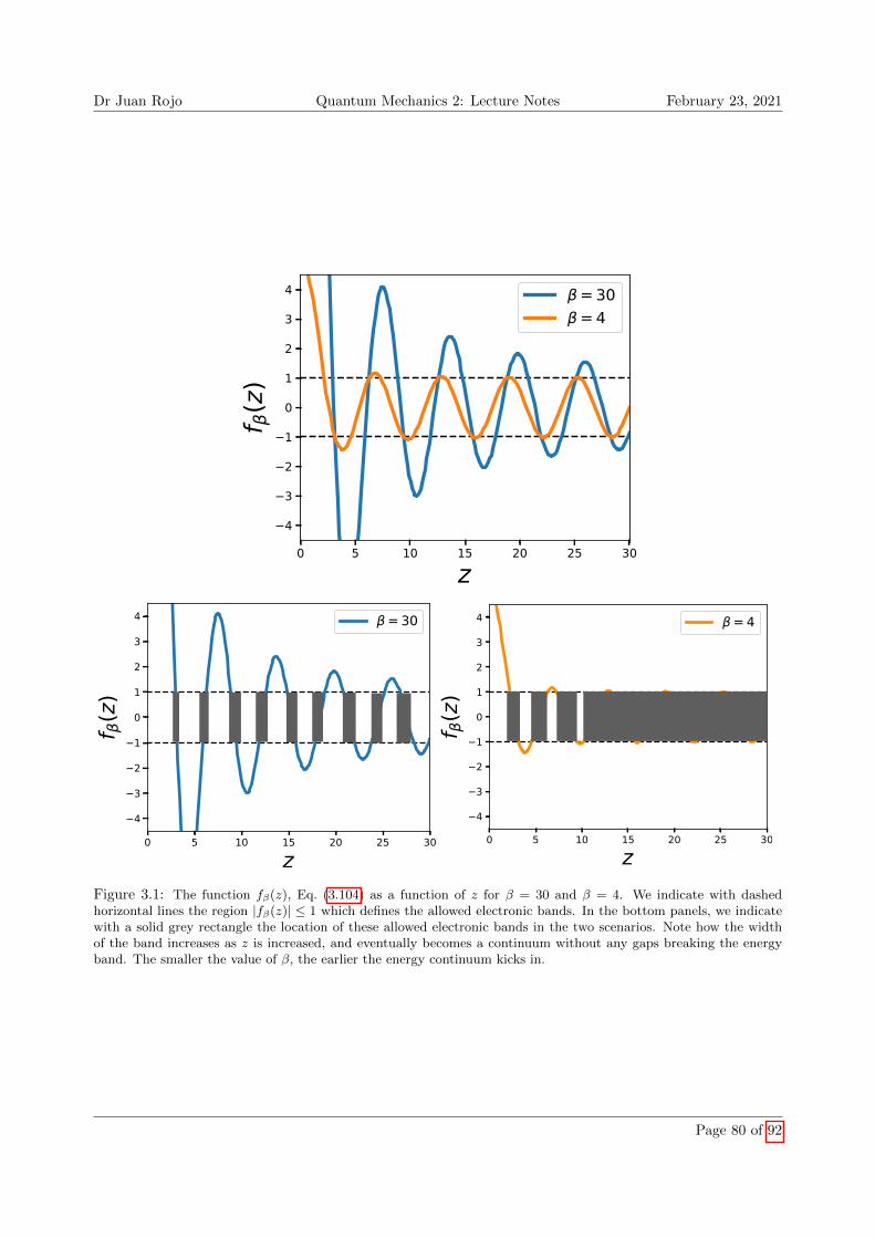
Fig. 3.1 displays the function f�(z), Eq. (3.104) as a function of z for � = 30 and � = 4. We indicate

with dashed horizontal lines the region |f�(z)| 1 which defines the allowed electronic bands. In the bottom

panels, we indicate with a solid grey rectangle the location of these allowed electronic bands in the two

scenarios. Note how the width of the band increases as z is increased, and eventually becomes a continuum

without any gaps breaking the energy band. Note also that smaller the value of �, the earlier the energy

continuum kicks in (since in � ! 0 limit the strength of the periodic potential vanishes).

Note also that in the limit � ! 0 we can always find a solution to Eq. (3.104): this means that in this

limit the energies are not quantised and can take any possible value. This is not unexpected, since for � ! 0

we recover the free particle system (subject to periodic boundary condition) and there we know that any

positive value of the energy is physically allowed.

Summary

We can now recapitulate what have we learned in this chapter concerning the quantum mechanics for systems

composed by identical particles:

I/ Quantum mechanics deals with truly indistinguishable particles: an electron is identical in all respects

to every other electron in the Universe.

II/ Systems composed by identical particles in quantum mechanics behave in a very di↵erent way as

compared to systems composed by distinguishable particles.

III/ Depending on their spin, particles can be classified into fermions and bosons. Bosons behave as if

they experienced some attractive interaction and tend to cluster together in the same quantum state.

Fermions, on the contrary, behave as if they experienced some repulsive interaction and tend to get far

for each other.

IV/ The Pauli exclusion principle for fermions tells us that a given quantum state can be occupied at most

by one fermion at the same time.

V/ The free electron gas model allows us to explain some important properties of solids, and shows how

there exists a quantum mechanical pressure from the fermion degeneracy that partially explains the

stability of solids.

VI/ The existence of continuous energy bands for the valence electrons in solids can be explained by the

presence of a periodic potential, where the electrons move, generated by the atomic cores sitting at

regularly-spaced locations within the crystalline lattice of a solid.

Page 79 of 92


Figure 3.1: The function f�(z), Eq. (3.104) as a function of z for � = 30 and � = 4. We indicate with dashedhorizontal lines the region |f�(z)| 1 which defines the allowed electronic bands. In the bottom panels, we indicatewith a solid grey rectangle the location of these allowed electronic bands in the two scenarios. Note how the widthof the band increases as z is increased, and eventually becomes a continuum without any gaps breaking the energyband. The smaller the value of �, the earlier the energy continuum kicks in.

Page 80 of 92

quantum mechanics 2 3 chapter 5: identical particles in

Documents