quantum mechanics in three dimensions - aheplphy240.ahepl.org/serway-9-qm-in-3d.pdf · quantum...

260

8Quantum Mechanicsin Three Dimensions

8.1 Particle in a Three-DimensionalBox

8.2 Central Forces and AngularMomentum

8.3 Space Quantization

8.4 Quantization of AngularMomentum and Energy(Optional)Lz Is Sharp: The Magnetic Quantum

Number

�L� Is Sharp: The Orbital QuantumNumber

E Is Sharp: The Radial WaveEquation

8.5 Atomic Hydrogen and Hydrogen-like IonsThe Ground State of Hydrogen-like AtomsExcited States of Hydrogen-like Atoms

8.6 Antihydrogen

Summary

Chapter Outline

So far we have shown how quantum mechanics can be used to describemotion in one dimension. Although the one-dimensional case illustrates suchbasic features of systems as the quantization of energy, we need a full three-dimensional treatment for the applications to atomic, solid-state, and nuclearphysics that we will meet in later chapters. In this chapter we extend the con-cepts of quantum mechanics from one to three dimensions and explore thepredictions of the theory for the simplest of real systems—the hydrogen atom.

With the introduction of new degrees of freedom (and the additionalcoordinates needed to describe them) comes a disproportionate increase inthe level of mathematical difficulty. To guide our inquiry, we shall rely on clas-sical insights to help us identify the observables that are likely candidates forquantization. These must come from the ranks of the so-called sharp observablesand, with few exceptions, are the same as the constants of the classical motion.

8.1 PARTICLE IN A THREE-DIMENSIONAL BOX

Let us explore the workings of wave mechanics in three dimensions throughthe example of a particle confined to a cubic “box.” The box has edge lengthL and occupies the region 0 � x, y, z � L, as shown in Figure 8.1. We assumethe walls of the box are smooth, so they exert forces only perpendicular to thesurface, and that collisions with the walls are elastic. A classical particle would

Copyright 2005 Thomson Learning, Inc. All Rights Reserved.

8.1 PARTICLE IN A THREE-DIMENSIONAL BOX 261

rattle around inside such a box, colliding with the walls. At each collision, thecomponent of particle momentum normal to the wall is reversed (changessign), while the other two components of momentum are unaffected (Fig.8.2). Thus, the collisions preserve the magnitude of each momentum compo-nent, in addition to the total particle energy. These four quantities—�px �, �py �,�pz �, and E —then, are constants of the classical motion, and it should be possi-ble to find quantum states for which all of them are sharp.1

The wavefunction � in three dimensions is a function of r and t. Again themagnitude of � determines the probability density P(r, t) � ��(r, t) �2, whichis now a probability per unit volume. Multiplication by the volume elementdV(�dx dy dz) gives the probability of finding the particle within the volumeelement dV at the point r at time t.

Since our particle is confined to the box, the wavefunction � must be zeroat the walls and outside. The wavefunction inside the box is found fromSchrödinger’s equation,

(8.1)

We see that �2/�x2 in the one-dimensional case is replaced in three dimen-sions by the Laplacian,

(8.2)

where U(r) is still the potential energy but is now a function of all the spacecoordinates: U(r) � U(x, y, z). Indeed, the Laplacian together with its multi-plying constant is just the kinetic energy operator of Table 6.2 extended to in-clude the contributions to kinetic energy from motion in each of three mutu-ally perpendicular directions:

(8.3)

This form is consistent with our belief that the Cartesian axes identify inde-pendent but logically equivalent directions in space. With this identification ofthe kinetic energy operator in three dimensions, the left-hand side of Equa-tion 8.1 is again the Hamiltonian operator [H ] applied to �, and the right-hand side is the energy operator [E] applied to � (see Section 6.8). As it doesin one dimension, Schrödinger’s equation asserts the equivalence of these twooperators when applied to the wavefunction of any physical system.

Stationary states are those for which all probabilities are constant in time,and are given by solutions to Schrödinger’s equation in the separable form,

� [Kx] � [Ky] � [Kz]

��2

2m�2 � ��

�2

2m

�2

�x2 � � ��2

2m

�2

�y2 � � ��2

2m

�2

�z2 �

�2 ��2

�x2 ��2

�y2 ��2

�z2

��2

2m�2� � U(r)� � i�

��

�t

z

xy

L

LL

Figure 8.1 A particle con-fined to move in a cubic box ofsides L. Inside the box U � 0.The potential energy is infiniteat the walls and outside the box.

1Recall from Section 6.7 that sharp observables are those for which there is no statistical distribu-tion of measured values. Indeed, quantum wavefunctions typically are labeled by the sharp ob-servables for that state. (For example, the oscillator states of Section 6.6 are indexed by the quan-tum number n, which specifies the sharp value of particle energy E. In this case, the sharp valuesof energy also are quantized, that is, limited to the discrete values (n � )�. It follows that anysharp observable is constant over time (unless the corresponding operator explicitly involvestime). The converse—that quantum states exist for which all constants of the classical motion aresharp—is not always true but occurs frequently enough that it can serve as a useful rule of thumb.

12

Figure 8.2 Change in particlevelocity (or momentum) dur-ing collision with a wall of thebox. For elastic collision with asmooth wall, the componentnormal to the wall is reversed,but the tangential componentsare unaffected.

v′

v

v||

v⊥

v||

–v⊥

Schrödinger equation in

three dimensions


�(r, t) � (r)e�it (8.4)

With this time dependence, the right-hand side of Equation 8.1 reduces to��, leaving (r) to satisfy the time-independent Schrödinger equation fora particle whose energy is E � �:

(8.5)

Since our particle is free inside the box, we take the potential energy U(r) � 0for 0 � x, y, z � L. In this case the spatial wavefunction also is separable; that is,solutions to Equation 8.5 with U(r) � 0 can be found in product form:

(r) � (x, y, z) � 1(x)2(y)3(z) (8.6)

Substituting Equation 8.6 into Equation 8.5 and dividing every term by thefunction (x, y, z) gives (for U(r) � 0)

In this form the independent variables are isolated: the first term on the leftdepends only on x, the second only on y, and the third only on z. To satisfythe equation everywhere inside the cube, each of these terms must reduce to aconstant:

(8.7)

The stationary states for a particle confined to a cube are obtained from thesethree separate equations. The energies E1, E2, and E3 are separation con-stants and represent the energy of motion along the three Cartesian axes x, y,and z. Consistent with this identification, the Schrödinger equation requiresthat E1 � E2 � E3 � E.

The first of Equations 8.7 is the same as that for the infinite square well in onedimension. Independent solutions to this equation are sin k1x and cos k1x, where

is the wavenumber of oscillation. Only sin k1x satisfies the condi-tion that the wavefunction must vanish at the wall x � 0, however. Requiring thewavefunction to vanish also at the opposite wall x � L implies k1L � n1�, wheren1 is any positive integer. In other words, we must be able to fit an integral num-ber of half-wavelengths into our box along the direction marked by x. It followsthat the magnitude of particle momentum along this direction must be one ofthe special values

Identical considerations applied to the remaining two equations show thatthe magnitudes of particle momentum in all three directions are similarly

� px � � �k1 � n1��

L n1 � 1, 2, � � �

k1 � √2m E1/�2

��2

2m3

d23

dz2 � E3

��2

2m2

d22

dy2 � E2

��2

2m1

d21

dx2 � E1

��2

2m1

d21

dx2 ��2

2m2

d22

dy2 ��2

2m3

d23

dz2 � E

��2

2m�2(r) � U(r)(r) � E(r)

262 CHAPTER 8 QUANTUM MECHANICS IN THREE DIMENSIONS

The time-independent

Schrödinger equation



quantized:

n1 � 1, 2, . . .

n2 � 1, 2, . . . (8.8)

n3 � 1, 2, . . .

Notice that ni � 0 is not allowed, since that choice leads to a i that is alsozero and a wavefunction (r) that vanishes everywhere. Since the momentaare restricted this way, the particle energy (all kinetic) is limited to the follow-ing discrete values:

(8.9)

Thus, confining the particle to the cube serves to quantize its momentum andenergy according to Equations 8.8 and 8.9. Note that three quantum numbersare needed to specify the quantum condition, corresponding to the threeindependent degrees of freedom for a particle in space. These quantumnumbers specify the values taken by the sharp observables for this system.

Collecting the previous results, we see that the stationary states for this par-ticle are

�(x, y, z, t) � A sin(k1x)sin(k2y)sin(k3z)e�it for 0 � x, y, z � L

� 0 otherwise(8.10)

The multiplier A is chosen to satisfy the normalization requirement. Example8.1 shows that A � (2/L)3/2 for the ground state, and this result continues tohold for the excited states as well.

E �1

2m(� px �2 � � py �2 � � pz �2) �

�2�2

2mL2 {n12 � n2

2 � n32 }

� pz � � �k3 � n3��

L

� py � � �k2 � n2��

L

� px � � �k1 � n1��

L

Using 2 sin2 � 1 � cos 2 gives

The same result is obtained for the integrations over y

and z. Thus, normalization requires

or

A � � 2

L �3/2

1 � A2 � L

2 �3

�L

0 sin2(�x/L)dx �

L

2�

L

4�sin(2�x/L) �

L

0�

L

2

EXAMPLE 8.1 Normalizing the BoxWavefunctions

Find the value of the multiplier A that normalizes the wave-function of Equation 8.10 having the lowest energy.

Solution The state of lowest energy is described byn1 � n2 � n3 � 1, or k1 � k2 � k3 � �/L. Since � isnonzero only for 0 � x, y, z � L, the probability densityintegrated over the volume of this cube must be unity:

� ��L

0 sin2(�z/L)dz�

� A2 ��L

0 sin2(�x/L)dx��L

0 sin2(�y/L)dy�

1 � �L

0dx �L

0dy �L

0dz � �(x, y, z, t) �2

Allowed values of

momentum components

for a particle in a box

Discrete energies allowed for

a particle in a box


Exercise 1 With what probability will the particle described by the wavefunction ofExample 8.1 be found in the volume 0 � x, y, z � L/4?

Answer 0.040, or about 4%

Exercise 2 Modeling a defect trap in a crystal as a three-dimensional box with edgelength 5.00 Å, find the values of momentum and energy for an electron bound to thedefect site, assuming the electron is in the ground state.

Answer �px � � �py � � �pz � � 1.24 keV/c; E � 4.51 eV

The ground state, for which n1 � n2 � n3 � 1, has energy

There are three first excited states, corresponding to the three different combi-nations of n1, n2, and n3, whose squares sum to 6. That is, we obtain the sameenergy for the three combinations n1 � 2, n2 � 1, n3 � 1, or n1 � 1, n2 � 2,n3 � 1, or n1 � 1, n2 � 1, n3 � 2. The first excited state has energy

Note that each of the first excited states is characterized by a different wave-function: 211 has wavelength L along the x-axis and wavelength 2L along they- and z-axes, but for 121 and 112 the shortest wavelength is along the y-axisand the z-axis, respectively.

Whenever different states have the same energy, this energy level is said tobe degenerate. In the example just described, the first excited level is three-fold (or triply) degenerate. This system has degenerate levels because of thehigh degree of symmetry associated with the cubic shape of the box. The de-generacy would be removed, or lifted, if the sides of the box were of unequallengths (see Example 8.3). In fact, the extent of splitting of the originally de-generate levels increases with the degree of asymmetry.

Figure 8.3 is an energy-level diagram showing the first five levels of aparticle in a cubic box; Table 8.1 lists the quantum numbers and degenera-cies of the various levels. Computer-generated plots of the probability den-sity �(x, y, z) �2 for the ground state and first excited states of a particle in abox are shown in Figure 8.4. Notice that the probabilities for the (degener-ate) first excited states differ only in their orientation with respect to thecoordinate axes, again a reflection of the cubic symmetry imposed by thebox potential.

E211 � E121 � E112 �6�2�2

2mL2

E111 �3�2�2

2mL2


Figure 8.3 An energy-level di-agram for a particle confined toa cubic box. The ground-stateenergy is E0 � 3�2�2/2mL2,and n2 � n1

2 � n22 � n3

2. Notethat most of the levels are de-generate.

12

11

9

6

3

4E0

E0

3E0

2E0

E0

11––3

None

3

3

3

None

Degeneracyn2

n2 � 2, n3 � 1 or n1 � 2, n2 � 1, n3 � 2 or n1 � 1,n2 � 2, n3 � 2. The corresponding wavefunctions insidethe box are

�221 � A sin� 2�x

L � sin� 2�y

L � sin� �z

L � e�iE221t/�

EXAMPLE 8.2 The Second Excited State

Determine the wavefunctions and energy for the secondexcited level of a particle in a cubic box of edge L. Whatis the degeneracy of this level?

Solution The second excited level corresponds tothe three combinations of quantum numbers n1 � 2,



Table 8.1 Quantum Numbers and Degeneracies

of the Energy Levels for a Particle

Confined to a Cubic Box*

n1 n2 n3 n2 Degeneracy

1 1 1 3 None

1 1 2 61 2 1 6 Threefold2 1 1 6

1 2 2 92 1 2 9 Threefold2 2 1 9

1 1 3 111 3 1 11 Threefold3 1 1 11

2 2 2 12 None

*Note : n2 � n12 � n2

2 � n32.

��

Ψ1112 Ψ2112 Ψ1212

(b)(a) (c)

xy xy xy

Figure 8.4 Probability density (unnormalized) for a particle in a box: (a) groundstate, ��111 �2; (b) and (c) first excited states, ��211 �2 and ��121 �2. Plots are for �� 2 inthe plane z � L. In this plane, ��112 �2 (not shown) is indistinguishable from ��111 �2.1

2

�122 � A sin� �x

L � sin� 2�y

L � sin� 2�z

L � e�iE122t/�

�212 � A sin� 2�x

L � sin� �y

L � sin� 2�z

L � e�iE212t/� The level is threefold degenerate, since each of thesewavefunctions has the same energy,

E221 � E212 � E122 �9�2�2

2mL2



8.2 CENTRAL FORCES AND ANGULAR MOMENTUM

The formulation of quantum mechanics in Cartesian coordinates is the nat-ural way to generalize from one to higher dimensions, but often it is not thebest suited to a given application. For instance, an atomic electron is attractedto the nucleus of the atom by the Coulomb force between opposite charges.This is an example of a central force, that is, one directed toward a fixedpoint. The nucleus is the center of force, and the coordinates of choice hereare spherical coordinates r, , � centered on the nucleus (Fig. 8.5). If thecentral force is conservative, the particle energy (kinetic plus potential) stays

The allowed energies are

The lowest energy occurs again for n1 � n2 � n3 � 1. In-creasing one of the integers by 1 gives the next-lowest, orfirst, excited level. If L1 is the largest dimension, thenn1 � 2, n2 � 1, n3 � 1 produces the smallest energy in-crement and describes the first excited state. Further, solong as both L2 and L3 are not equal to L1, the first ex-cited level is nondegenerate, that is, there is no otherstate with this energy. If L 2 or L3 equals L1, the level isdoubly degenerate; if all three are equal, the level will betriply degenerate. Thus, the higher the symmetry, themore degeneracy we find.

��2�2

2m �� n1

L1�

2

� � n2

L2�

2

� � n3

L3�

2

�E � (� px �2 � � py �2 � � pz �2)/2m

EXAMPLE 8.3 Quantization in a Rectangular Box

Obtain a formula for the allowed energies of a particleconfined to a rectangular box with edge lengths L1, L2,and L3. What is the degeneracy of the first excited state?

Solution For a box having edge length L1 in the x di-rection, will be zero at the walls if L1 is an integralnumber of half-wavelengths. Thus, the magnitude of par-ticle momentum in this direction is quantized as

Likewise, for the other two directions, we have

� pz � � �k3 � n3��

L3 n3 � 1, 2, � � �

� py � � �k2 � n2��

L2 n2 � 1, 2, � � �

� px � � �k1 � n1��

L1 n1 � 1, 2, � � �

Nucleus

Electron

z = r cosθ

φ

x

z

y

r θ

x = r sin cosθ φ

y = r sin sinθ φ

r sinθ

Figure 8.5 The central force on an atomic electron is one directed toward a fixedpoint, the nucleus. The coordinates of choice here are the spherical coordinates r, , �

centered on the nucleus.


8.2 CENTRAL FORCES AND ANGULAR MOMENTUM 267

constant and E becomes a candidate for quantization. In that case, the quan-tum states are stationary waves (r)e�it, with � E/�, where E is the sharpvalue of particle energy.

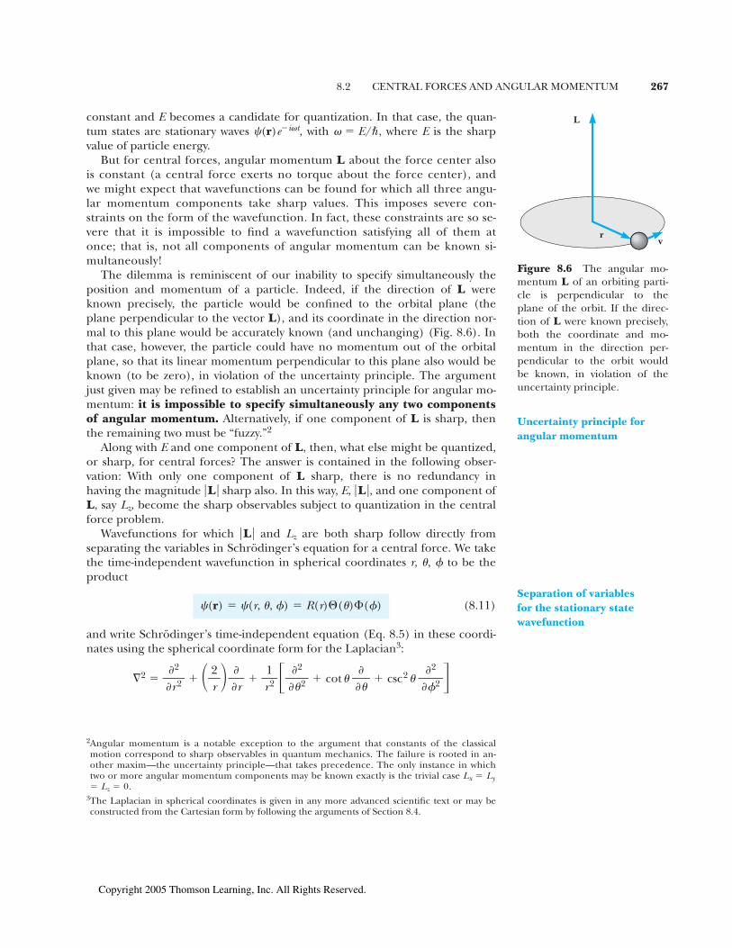
But for central forces, angular momentum L about the force center alsois constant (a central force exerts no torque about the force center), andwe might expect that wavefunctions can be found for which all three angu-lar momentum components take sharp values. This imposes severe con-straints on the form of the wavefunction. In fact, these constraints are so se-vere that it is impossible to find a wavefunction satisfying all of them atonce; that is, not all components of angular momentum can be known si-multaneously!

The dilemma is reminiscent of our inability to specify simultaneously theposition and momentum of a particle. Indeed, if the direction of L wereknown precisely, the particle would be confined to the orbital plane (theplane perpendicular to the vector L), and its coordinate in the direction nor-mal to this plane would be accurately known (and unchanging) (Fig. 8.6). Inthat case, however, the particle could have no momentum out of the orbitalplane, so that its linear momentum perpendicular to this plane also would beknown (to be zero), in violation of the uncertainty principle. The argumentjust given may be refined to establish an uncertainty principle for angular mo-mentum: it is impossible to specify simultaneously any two componentsof angular momentum. Alternatively, if one component of L is sharp, thenthe remaining two must be “fuzzy.”2

Along with E and one component of L, then, what else might be quantized,or sharp, for central forces? The answer is contained in the following obser-vation: With only one component of L sharp, there is no redundancy inhaving the magnitude �L � sharp also. In this way, E, �L �, and one component ofL, say Lz, become the sharp observables subject to quantization in the centralforce problem.

Wavefunctions for which �L � and Lz are both sharp follow directly fromseparating the variables in Schrödinger’s equation for a central force. We takethe time-independent wavefunction in spherical coordinates r, , � to be theproduct

(8.11)

and write Schrödinger’s time-independent equation (Eq. 8.5) in these coordi-nates using the spherical coordinate form for the Laplacian3:

�2 ��2

�r2 � � 2

r ��

�r�

1

r2 � �2

� 2 � cot �

� � csc2

�2

��2 �

(r) � (r, , �) � R(r)�( )�(�)

L

rv

Figure 8.6 The angular mo-mentum L of an orbiting parti-cle is perpendicular to theplane of the orbit. If the direc-tion of L were known precisely,both the coordinate and mo-mentum in the direction per-pendicular to the orbit wouldbe known, in violation of theuncertainty principle.

2Angular momentum is a notable exception to the argument that constants of the classicalmotion correspond to sharp observables in quantum mechanics. The failure is rooted in an-other maxim—the uncertainty principle—that takes precedence. The only instance in whichtwo or more angular momentum components may be known exactly is the trivial case Lx � Ly

� Lz � 0.3The Laplacian in spherical coordinates is given in any more advanced scientific text or may beconstructed from the Cartesian form by following the arguments of Section 8.4.

Uncertainty principle for

angular momentum

Separation of variables

for the stationary state

wavefunction


After dividing each term in Equation 8.5 by R��, we are left with

Notice that ordinary derivatives now replace the partials and that U(r)becomes simply U(r) for a central force seated at the origin. We can isolate thedependence on � by multiplying every term by r 2sin2 to get, after some re-arrangement,

(8.12)

In this form the left side is a function only of � while the right side dependsonly on r and . Because these are independent variables, equality of the twosides requires that each side reduce to a constant. Following convention, wewrite this separation constant as �m�

2, where m� is the magnetic quantumnumber.4

Equating the left side of Equation 8.12 to �m�

2 gives an equation for �(�):

(8.13)

A solution to Equation 8.13 is �(�) � exp(im��); this is periodic with period2� if m� is restricted to integer values. Periodicity is necessary here because allphysical properties that derive from the wavefunction should be unaffected bythe replacement � : � � 2�, both of which describe the same point in space(see Fig. 8.5).

Equating the right side of Equation 8.12 to �m�

2 gives, after some furtherrearrangement,

(8.14)

In this form the variables r and are separated, the left side being a func-tion only of r and the right side a function only of . Again, each side mustreduce to a constant. This furnishes two more equations, one for each of theremaining functions R(r) and �( ), and introduces a second separation

�m�

2

sin2

r2

R � d2R

dr2 �2

r

dR

dr � �2mr2

�2 [E � U(r)] � �1

� � d2�

d 2 � cot d�

d �

d2�

d�2 � �m�

2�(�)

�2mr2

�2 [E � U(r)]�

1

�

d2�

d�2 � �sin2 � r2

R � d2R

dr2 �2

r

dR

dr � �1

� � d2�

d 2 � cot d�

d �

��2

2m�

1

r2 sin2

d2�

d�2 � U(r) � E

��2

2mR � d2R

dr2 �2

r

dR

dr � ��2

2m�

1

r2 � d2�

d 2 � cot d�

d �


4This seemingly peculiar way of writing the constant multiplier is based on the physical signifi-cance of the function �(�) and is discussed at length in (optional) Section 8.4. The student is re-ferred there for a concise treatment of the quantum central force problem based on the operatormethods of Section 6.8.


8.2 CENTRAL FORCES AND ANGULAR MOMENTUM 269

constant, which we write as �(� � 1). Equating the right side of Equation 8.14to �(� � 1) requires �( ) to satisfy

(8.15)

� is called the orbital quantum number. For (r) to be an acceptablewavefunction, �( ) also must be bounded and single-valued, conditionswhich are met for functions satisfying Equation 8.15 only if � is a nonnega-tive integer, and then only if m� is limited to absolute values not larger than�. The resulting solutions �( ) are polynomials in cos known as associ-ated Legendre polynomials. A few of these polynomials are listed in Table8.2 for easy reference. The products �( )�(�) specify the full angular de-pendence of the central force wavefunction and are known as sphericalharmonics, denoted by . Some spherical harmonics are given inTable 8.3. The constant prefactors are chosen to normalize thesefunctions.5

Y �

m� ( , �)

d2�

d 2 � cot d�

d � m�

2 csc2 �( ) � ��(� � 1)�( )

5The normalization is such that the integral of over the surface of a sphere with unitradius is 1.

� Y �m� �2

Table 8.2 Some

Associated

Legendre

Polynomials

P�m�(cos �)

P00 � 1

P10 � 2 cos

P11 � sin

P20 � 4(3 cos2 � 1)

P21 � 4 sin cos

P 22 � sin2

P30 � 24(5 cos3 � 3 cos )

P31 � 6 sin (5 cos2 � 1)

P32 � 6 sin2 cos

P33 � sin3

Table 8.3 The Spherical Harmonics Y�m�(�, �)

Y 3�3 � �1

8 √ 35

��sin3 �e�3i�

Y 3�2

� 14 √ 105

2�� sin2 �cos � e�2i�

Y 3�1

� �18 √ 21

��sin �(5cos2 � 1) � e�i�

Y 30 � 1

4 √ 7

��(5 cos3 � 3cos )

Y 2�2

� 14 √ 15

2�� sin2 � e�2i�

Y 2�1

� �12 √ 15

2��sin �cos � e�i�

Y 20

� 14 √ 5

��(3 cos2 � 1)

Y 1�1

� �12 √ 3

2�� sin � e�i�

Y 10 � 1

2√ 3

��cos

Y 00 �

1

2√�



In keeping with our earlier remarks, the separation constants �(� � 1) andm� should relate to the sharp observables �L �, Lz, and E for central forces. Theconnection is established by the more detailed arguments of Section 8.4, withthe result

� � 0, 1, 2, . . .

Lz � m�� m� � 0, �1, �2, . . . , �� (8.16)

We see that the limitation on the magnetic quantum number m� to values be-tween �� and ��, obtained on purely mathematical grounds from separatingvariables, has an obvious physical interpretation: the z component of angularmomentum, Lz, must never exceed the magnitude of the vector, �L �! Notice,too, that � and m� are quantum numbers for angular momentum only; theirconnection with particle energy E must depend on the potential energy func-tion U(r) and is prescribed along with the radial wavefunction R(r) in the finalstage of the separation procedure.

To obtain R(r), we return to Equation 8.14 and equate the left side to�(� � 1). Rearranging terms once more, we find that R(r) must satisfy

(8.17)

This is the radial wave equation; it determines the radial part of thewavefunction � and the allowed particle energies E. As the equation containsthe orbital quantum number �, each angular momentum orbital is expectedto give rise to a different radial wave and a distinct energy. By contrast, themagnetic quantum number m� appears nowhere in this equation. Thus, theradial wave and particle energy remain the same for different m� values consis-tent with a given value of �. In particular, for a fixed � the particle energy Eis independent of m�, and so is at least 2� �1-fold degenerate. Such de-generacy—a property of all central forces—stems from the spherical symmetryof the potential and illustrates once again the deep-seated connection be-tween symmetry and the degeneracy of quantum states.

The reduction from Schrödinger’s equation to the radial wave equationrepresents enormous progress and is valid for any central force. Still, the taskof solving this equation for a specified potential U(r) is a difficult one, oftenrequiring methods of considerable sophistication. In Section 8.5 we tackle thistask for the important case of the electron in the hydrogen atom.

��2

2m � d2R

dr2 �2

r

dR

dr � ��(� � 1)�2

2mr2 R(r) � U(r)R(r) � ER(r)

� L � � √�(� � 1)�Angular momentum and its z

component are quantized

Radial wave equation

The corresponding angular momentum has magnitude

�L � � mvR � (1.00 kg)(6.28 m/s)(1.00 m)

� 6.28 kg � m2/s

But angular momentum is quantized as which is approximately �� when � is large. Then

� �� L ��

�6.28 kg�m2/s

1.055 � 10�34 kg�m2/s� 5.96 � 1034

√�(� � 1)�,

EXAMPLE 8.4 Orbital Quantum Number for a Stone

A stone with mass 1.00 kg is whirled in a horizontal circleof radius 1.00 m with a period of revolution equal to1.00 s. What value of orbital quantum number � de-scribes this motion?

Solution The speed of the stone in its orbit is

v �2R

T�

2(1.00 m)

1.00 s� 6.28 m/s


8.3 SPACE QUANTIZATION 271

8.3 SPACE QUANTIZATION

For wavefunctions satisfying Equations 8.13 and 8.15, the orbital angular mo-mentum magnitude �L �, and Lz, the projection of L along the z-axis, are bothsharp and quantized according to the restrictions imposed by the orbital andmagnetic quantum numbers, respectively. Together, � and m� specify theorientation of the angular momentum vector L. The fact that the direction ofL is quantized with respect to an arbitrary axis (the z-axis) is referred to asspace quantization.

Let us look at the possible orientations of L for a given value of orbitalquantum number �. Recall that m� can have values ranging from �� to ��. If� � 0, then m� � 0 and Lz � 0. In fact, for this case �L � � 0, so that all compo-nents of L are 0. If � � 1, then the possible values for m� are �1, 0, and �1, sothat Lz may be ��, 0, or ��. If � � 2, m� can be �2, �1, 0, �1, or �2, corre-sponding to Lz values of �2�, ��, 0, ��, or �2�, and so on. A classical visual-ization of the algebra describing space quantization for the case � � 2 isshown in Figure 8.7a. Note that L can never be aligned with the z-axis, since Lz

must be smaller than the total angular momentum L. From a three-dimen-sional perspective, L must lie on the surface of a cone that makes an angle with the z-axis, as shown in Figure 8.7b. From the figure, we see that also isquantized and that its values are specified by the relation

(8.18)

Classically, can take any value; that is, the angular momentum vector L canpoint in any direction whatsoever. According to quantum mechanics, thepossible orientations for L are those consistent with Equation 8.18. Further-more, these special directions have nothing to do with the forces acting on

cos �Lz

� L ��

m�

√�(� � 1)

In fairness to Bohr, we should point out that theBohr model makes no distinction between the quanti-zation of L and quantization of its components alongthe coordinate axes. From the classical viewpoint, thecoordinate system can always be oriented to align oneof the axes, say the z-axis, along the direction of L. Inthat case, L may be identified with �Lz�. The Bohr postu-late in this form agrees with the quantization of Lz inEquation 8.16 and indicates � � 1 for the first Bohr or-bit! This conflicting result derives from a false asser-tion, namely, that we may orient a coordinate axisalong the direction of L. The freedom to do so must beabandoned if the quantization rules of Equation 8.16are correct! This stunning conclusion is one of thegreat mysteries of quantum physics and is implicit inthe notion of space quantization that we discuss in thenext section.

Again, we see that macroscopic objects are described byenormous quantum numbers, so that quantization is notevident on this scale.

EXAMPLE 8.5 The Bohr Atom Revisited

Discuss angular momentum quantization in the Bohrmodel. What orbital quantum number describes the elec-tron in the first Bohr orbit of hydrogen?

Solution Angular momentum in the Bohr atom isquantized according to the Bohr postulate

�L � � mvr � n�

with n � 1 for the first Bohr orbit. Comparing this with thequantum mechanical result, Equation 8.14, we see that thetwo rules are incompatible! The magnitude �L� can neverbe an integral multiple of �—the smallest nonzero valueconsistent with Equation 8.16 is for � � 1.� L � � √2�

The orientations of L are

restricted (quantized)



the particle, provided only that these forces are central. Thus, the rule ofEquation 8.18 does not originate with the law of force but derives fromthe structure of space itself, hence the name space quantization.

Figure 8.7 is misleading in showing L with a specific direction, for which allthree components Lx, Ly, and Lz are known exactly. As we have mentioned,there is no quantum state for which this condition is true. If Lz is sharp, thenLx and Ly must be fuzzy. Accordingly, it is more proper to visualize the vector Lof Figure 8.7b as precessing around the z-axis so as to trace out a cone inspace. This allows the components Lx and Ly to change continually, while Lz

maintains the fixed value m��.6

Finally, we obtain the allowed values of from

Substituting the values for m� gives

cos � �0.866, �0.577, �0.289, and 0

or

� �30�, �54.8�, �73.2�, and 90�

cos �Lz

� L ��

m�

2√3

EXAMPLE 8.6 Space Quantization for anAtomic Electron

Consider an atomic electron in the � � 3 state. Calculatethe magnitude �L � of the total angular momentum andthe allowed values of Lz and .

Solution With � � 3, Equation 8.16 gives

The allowed values of Lz are m��, with m� � 0, �1, �2,and �3. This gives

Lz � �3�, �2�, ��, 0, �, 2�, 3�

� L � � √3(3 � 1)� � 2√3�

� = 2

z

Lz = 0

Lz = –2h

Lz = –h

Lz = h

Lz = 2h

|L | = 6h√

(a) (b)

Lz = 0

Lz = –2h

Lz = –h

Lz = h

Lz = 2h

z

LθLz

Figure 8.7 (a) The allowed projections of the orbital angular momentum for thecase � � 2. (b) From a three-dimensional perspective, the orbital angular momentumvector L lies on the surface of a cone. The fuzzy character of Lx and Ly is depicted byallowing L to precess about the z-axis, so that Lx and Ly change continually while Lz

maintains the fixed value m��.

6This precession of the classical vector to portray the inherent fuzziness in Lx and Ly is meant tobe suggestive only. In effect, we have identified the quantum averages Lx� and Ly� with theiraverages over time in a classical picture, but the two kinds of averaging in fact are quite distinct.


8.4 QUANTIZATION OF ANGULAR MOMENTUM AND ENERGY 273

Exercise 3 Compare the minimum angles between L and the z-axis for the electronof Example 8.6 and for the 1.00-kg stone of Example 8.4.

Answer 30� for the electron but only 2.3 � 10�16 degrees for the stone

8.4 QUANTIZATION OF ANGULARMOMENTUM AND ENERGY

We saw in Section 8.2 that angular momentum plays an essential role in the quantiza-

tion of systems with spherical symmetry. Here we develop further the properties of

angular momentum from the viewpoint of quantum mechanics and show in more

detail how angular momentum considerations facilitate the solution to Schrödinger’s

equation for central forces.

Our treatment is based on the operator methods introduced in Section 6.8,

which the reader should review at this time. In particular, the eigenvalue condition

[Q ]� � q� (8.19)

used there as a test for sharp observables becomes here a tool for discovering the

form of the unknown wavefunction �. (Recall that [Q ] denotes the operator for

some observable Q and q is the sharp value of that observable when measured for a

system described by the wavefunction �.) We look on Equation 8.19 now as a con-

straint imposed on the wavefunction � that guarantees that the observable Q will

take the sharp value q in that state. The more sharp observables we can identify for

some system, the more we can learn in advance about the wavefunction describing

that system. With few exceptions, the sharp observables are just those that areconstants of the classical motion. (See footnote 1.)

Consider the particle energy. If total energy is constant, we should be able to find

wavefunctions � for which E is a sharp observable. Otherwise, repeated measure-

ments made on identical systems would reveal a statistical distribution of values for

the particle energy, inconsistent with the idea of a quantity not changing over time.

Thus, energy conservation suggests �E � 0, which, in turn, requires � to be an

eigenfunction of the energy operator

[E]� � E �

Because [E] � i��/�t this eigenvalue condition is met by the stationary waves

(r)e�it, with E � � the sharp value of particle energy.

The argument for energy applies equally well to other constants of the classical

motion.7 If the only forces are central, angular momentum about the force center is

a constant of the motion. This is a vector quantity L � r � p, whose rectangular

components are expressed in terms of position and momentum components as

Lz � (r � p)z � xpy � ypx

and so on. In the same way, the operators for angular momentum are found from the

coordinate and momentum operators. From Chapter 6, the operator for x is just the

O P T I O N A L

7Exceptions to this rule do exist. For instance, an atomic electron cannot have all three angularmomentum components sharp at once, even though in this case all components are constantclassically. For such incompatible observables, quantum mechanics adopts the broader interpreta-tion of a conserved quantity as one whose average value does not change over time, no matter whatmay be the initial state of the system. With this definition, all components of angular momentumfor an atomic electron remain constant, but no more than one can be sharp in a given state.


coordinate itself, and the operator for momentum in this direction is (�/i) �/�x.

Similar relations should apply to the directions labeled y and z,8 so that the operator

for Lz becomes

(8.20)

Angular momentum finds its natural expression in the spherical coordinates

of Figure 8.5. A little geometry applied to Figure 8.5 shows that the spherical-to-

Cartesian coordinate transformation equations are

z � r cos

x � r sin cos� (8.21)

y � r sin sin�

The inverse transformations are

(8.22)

The procedure for transcribing operators such as [Lz ] from Cartesian to spherical

form is straightforward, but tedious. For instance, an application of the chain rule gives

for any function f. On the left we think of f expressed as a function of x, y, z, but on

the right the same function is expressed in terms of r, , �. The partial derivatives

�r/�z, and so on, are to be taken with the aid of the transformation equations, hold-

ing x and y fixed. The simplest of these is ��/�z . From the inverse transformations

in Equations 8.22, we see that � is independent of z, so that ��/�z � 0. From the

same equations we find that

To obtain � /�z we differentiate the second of Equations 8.22 implicitly to get

Converting the right-hand side back to spherical coordinates gives

or � /�z � �sin /r. Collecting the previous results, we have

�

�z�

�r

�z

�

�r�

�

�z

�

� � cos

�

�r�

sin

r

�

�

�sin �

�z� �

(r cos )2

r3 �1

r�

1 � cos2

r�

sin2

r

�sin �

�z�

�{cos }

�z� z(�1

2){x2 � y2 � z2}�3/2(2z) � {x2 � y2 � z2}�1/2

�r

�z�

1

2 {x2 � y2 � z2}�1/2(2z) �

z

r� cos

�f

�z�

�r

�z

�f

�r�

�

�z

�f

� �

��

�z

�f

��

tan� �y

x

cos �z

r� z {x2 � y2 � z2}�1/2

r � {x2 � y2 � z2}1/2

[Lz] � [x][py] � [y][px] ��

i �x�

�y� y

�

�x �


8For the momentum operator along each axis we use the one-dimensional form from Chapter6, ([px] � (�/i)�/�x, etc.), consistent with the belief that Cartesian axes identify independentbut logically equivalent directions in space.


8.4 QUANTIZATION OF ANGULAR MOMENTUM AND ENERGY 275

In like fashion, we can obtain spherical representations for �/�x, �/�y and ulti-

mately for the angular momentum operators themselves:

(8.23)

Notice that the operators for angular momentum in spherical form do not contain

the radial coordinate r—our reward for selecting the right system of coordinates! By

insisting that angular momentum be sharp in the quantum state �, and using the

differential forms (Eqs. 8.23) for the angular momentum operators, we can discover

how the wavefunction depends on the spherical angles and � without knowing the

details of the central force.

Lz Is Sharp: The Magnetic Quantum Number

For Lz to be sharp, our wavefunction � � (r)e�it must be an eigenfunction of

[L z], or

(8.24)

with Lz the eigenvalue (a number). Equation 8.24 prescribes the functional depen-

dence of on the azimuthal angle � to be

(8.25)

with C still any function of r and . The values taken by Lz must be restricted, however.

Since increasing � by 2� radians returns us to the same place in space (see Fig. 8.5),

the wavefunction also should return to its initial value, that is, the solutions repre-

sented by Equation 8.25 must be periodic in � with period 2�. This will be true if Lz/�

is any integer, say, m� or Lz � m��. The magnetic quantum number m� indicates the

(sharp) value for the z component of angular momentum in the state described by .

Because all components of L are constant for central forces, we should continue

by requiring the wavefunction of Equation 8.25 also to be an eigenfunction of the

operator for a second angular momentum component, say [Lx], so that Lz and Lx

might both be sharp in the state . For to be an eigenfunction of [Lx] with eigen-

value Lx requires

This relation must hold for all values of and �. In particular, for � � 0 the re-

quirement is

Because varies exponentially with � according to Equation 8.25, the indicated de-

rivative may be taken and evaluated at � � 0 to get

(�Lz cot ) � Lx

which can be satisfied for all only if Lx � Lz � 0 or if vanishes identically. A simi-

lar difficulty arises if we attempt to make Ly sharp together with Lz. Therefore,

i�cot �

�� Lx

i� �sin��

� � cot cos �

�

�� Lx

(r) � CeiLz�/�

�i��

�� Lz

[Lz] � �i��

��

[Ly] � �i� �cos��

� � cot sin �

�

��

[Lx] � i� �sin��

� � cot cos �

�

��


unless the angular momentum is exactly zero (all components), there is nowavefunction for which two or more components are simultaneously sharp!

�L � Is Sharp: The Orbital Quantum Number

To make further progress, we must look to other constants of the classical motion.

In addition to each component of angular momentum, the magnitude �L � of the

vector also is constant and becomes a candidate for an observable that can be made

sharp together with Lz. Consider simply the squared-magnitude L2 � L � L. The

operator for L2 is

[L]2 � [Lx]2 � [Ly]

2 � [Lz]2

Using Equation 8.23, we find the spherical coordinate form for [L2]:

(8.26)

For L2 to be sharp requires or

But from Equation 8.24, we see that differentiating with respect to � is equivalent

to multiplication by iLz/� � im�, so that the last equation reduces to

(8.27)

For wavefunctions satisfying Equation 8.27, the magnitude of angular momen-

tum will be sharp at the value �L �. The equation prescribes the dependence of on

the polar angle . The solutions are not elementary functions but can be investi-

gated with the help of more advanced techniques. The results of such an investiga-

tion are reported in Section 8.2 and repeated here for completeness: Physically

acceptable solutions to Equation 8.27 can be found provided ,

where �, the orbital quantum number, must be a nonnegative integer. Furthermore,

the magnetic quantum number, also appearing in Equation 8.27, must be limited as

�m� � � �. With these restrictions, the solutions to Equation 8.27 are the associated

Legendre polynomials in cos , denoted . Several of these polynomials are

listed in Table 8.2 for easy reference; you may verify by direct substitution that they

satisfy Equation 8.27 for the appropriate values of � and m�.

The associated Legendre polynomials may be multiplied by exp(im��) and still

satisfy the orbital equation Equation 8.27. Indeed, the products exp(im��)

satisfy both Equations 8.24 and 8.27; thus, they represent waves for which �L � and Lz

are simultaneously sharp. Except for a multiplicative constant, these are just the

spherical harmonics introduced in Section 8.2.

E Is Sharp: The Radial Wave Equation

For energy to be constant, E should be a sharp observable. The stationary state form

�(r, t) � (r)e�it results from imposing the eigenvalue condition for the energy

operator [E ]—but what of the other energy operator [H ] � [K ] � [U ] (the

Hamiltonian)? In fact, requiring [H ]� � E � is equivalent to writing the time-

independent Schrödinger equation for (r)

(8.28)��2

2m�2 � U(r) � E

Y �

m�( , �)

P�

m�(cos )

P�

m�(cos )

� L � � √�(� � 1)�

��2 � �2

� 2 � cot �

� � m�

2csc2 � � � L �2

��2 � �2

� 2 � cot �

� � csc2

�2

��2 � � � L �2

[L2] � � L �2

[L2] � ��2 � �2

� 2 � cot �

� � csc2

�2

��2 �



8.5 ATOMIC HYDROGEN AND HYDROGEN-LIKE IONS 277

because [U ] � U(r) and the kinetic energy operator [K] in three dimensions is

none other than

The spherical form of the Laplacian given in Section 8.2 may be used to write

[K ] in spherical coordinates:

Comparing this with the spherical representation for [L2] from Equation 8.26 shows

that [K ] is the sum of two terms,

(8.29)

representing the separate contributions to the kinetic energy from the orbital and

radial components of motion. The comparison also furnishes the spherical form for

[Krad]:

(8.30)

These expressions for [K ] are completely general. When applied to waves

for which �L � is sharp, however, the operator [L2] may be replaced with the number

�L�2 � �(� � 1)�2. Therefore, the Schrödinger equation (Eq. 8.28) becomes

(8.31)

For central forces, all terms in this equation, including U(r), involve only the spheri-

cal coordinate r : the angle variables and � have been eliminated from further con-

sideration by the requirement that be an eigenfunction of [L2]! It follows that the

solutions to Equation 8.31 take the form of a radial wave R(r) multiplied by a spher-

ical harmonic:

(8.32)

The spherical harmonic may be divided out of each term in Equation 8.31, in effect

replacing (r) by R(r). The result is just the radial wave equation of Section 8.2; it

determines the radial wavefunction R(r) and the allowed particle energies E, once

the potential energy function U(r) is specified.

8.5 ATOMIC HYDROGEN AND HYDROGEN-LIKE IONS

In this section we study the hydrogen atom from the viewpoint of wavemechanics. Its simplicity makes atomic hydrogen the ideal testing ground forcomparing theory with experiment. Furthermore, the hydrogen atom is theprototype system for the many complex ions and atoms of the heavierelements. Indeed, our study of the hydrogen atom ultimately will enable usto understand the periodic table of the elements, one of the greatest triumphsof quantum physics.

The object of interest is the orbiting electron, with its mass m and charge�e, bound by the force of electrostatic attraction to the nucleus, with itsmuch larger mass M and charge �Ze, where Z is the atomic number. The

(r) � R(r)Y �

m� ( , �)

[Krad](r) ��(� � 1)�2

2mr2 (r) � U(r)(r) � E(r)

[Krad] � ��2

2m � �2

�r2 �2

r

�

�r �

[K] � [Krad] � [Korb] � [Krad] �1

2mr2 [L2]

[K] � ��2

2m � �2

�r2 �2

r

�

�r�

1

r2 � �2

� 2 � cot �

� � csc2

�2

��2 ��

[K] �[px]

2 � [py]2 � [pz]

2

2m�

(�/i)2{(�/�x)2 � (�/�y)2 � (�/�z)2}

2m� �

�2

2m�2


choice Z � 1 describes the hydrogen atom, while for singly ionized helium(He�) and doubly ionized lithium (Li2�), we take Z � 2 and Z � 3, respec-tively, and so on. Ions with only one electron, like He� and Li2�, are calledhydrogen-like. Because M �� m, we will assume that the nucleus does notmove but simply exerts the attractive force that binds the electron. This forceis the coulomb force, with its associated potential energy

(8.33)

where k is the coulomb constant.The hydrogen atom constitutes a central force problem; according to Sec-

tion 8.2, the stationary states for any central force are

(8.34)

where is a spherical harmonic from Table 8.3. The radial wavefunc-tion R(r) is found from the radial wave equation of Section 8.2,

(8.17)

U(r) is the potential energy of Equation 8.33; the remaining terms on the leftof Equation 8.17 are associated with the kinetic energy of the electron. Theterm proportional to �(� � 1)�2 � (�L2 �) is the orbital contribution to kineticenergy, Korb. To see this, consider a particle in circular orbit, in which all thekinetic energy is in orbital form (since the distance from the center remainsfixed). For such a particle and �L � � mvr. Eliminating the parti-cle speed v, we get

(8.35)

Although it was derived for circular orbits, this result correctly represents theorbital contribution to kinetic energy of a mass m in general motion withangular momentum L.9

The derivative terms in Equation 8.17 are the radial contribution to thekinetic energy, that is, they represent the contribution from electron motiontoward or away from the nucleus. The leftmost term is just what we shouldwrite for the kinetic energy of a matter wave � R(r) associated with motionalong the coordinate line marked by r. But what significance should we attachto the first derivative term dR/dr? In fact, the presence of this term is evidencethat the effective one-dimensional matter wave is not R(r), but rR(r). In support ofthis claim we note that

Then the radial wave equation written for the effective one-dimensionalmatter wave g(r) � rR(r) takes the same form as Schrödinger’s equation in

d2(rR)

dr2 � r � d2R

dr2 �2

r

dR

dr �

Korb �m

2 � � L �mr �

2

�� L �2

2mr2

Korb � 12 mv2

��2

2m � d2R

dr2 �2

r

dR

dr � ��(� � 1)�2

2mr2 R(r) � U(r)R(r) � ER(r)

Y�m�( , �)

�(r, , �, t) � R(r)Y�m�( , �)e�it

U(r) �k(�Ze)(�e)

r� �

kZe2

r


9For any planar orbit we may write �L � � rp�, where p� is the component of momentum in theorbital plane that is normal to the radius vector r. The orbital part of the kinetic energy is thenKorb � p�

2/2m � �L �2/2mr 2.



one dimension,

(8.36)

but with an effective potential energy

(8.37)

The magnitude of g(r) also furnishes probabilities, as described later in thissection.

The solution of Equation 8.36 with U(r) � �kZe2/r (for one-electron atomsor ions) requires methods beyond the scope of this text. Here, as before, weshall present the results and leave their verification to the interested reader.Acceptable wavefunctions can be found only if the energy E is restricted to beone of the following special values:

n � 1, 2, 3, . . . (8.38)

This result is in exact agreement with that found from the simple Bohr theory(see Chapter 4): a0 � �2/meke2 is the Bohr radius, 0.529 Å, and ke2/2a0 is theRydberg energy, 13.6 eV. The integer n is called the principal quantum num-ber. Although n can be any positive integer, the orbital quantum number nowis limited to values less than n; that is, � can have only the values

(8.39)

The cutoff at (n � 1) is consistent with the physical significance of these quan-tum numbers: The magnitude of orbital angular momentum (fixed by �) can-not become arbitrarily large for a given energy (fixed by n). A semiclassical ar-gument expressing this idea leads to �max � n � 1 (see Problem 20). In thesame spirit, the restriction on the magnetic quantum number m� to values be-tween �� and �� guarantees that the z component of angular momentumnever exceeds the magnitude of the vector.

The radial waves R(r) for hydrogen-like atoms are products of exponentialswith polynomials in r/a0. These radial wavefunctions are tabulated as Rn�(r) inTable 8.4 for principal quantum numbers up to and including n � 3.

For hydrogen-like atoms, then, the quantum numbers are n, �, and m�, as-sociated with the sharp observables E, �L �, and Lz, respectively. Notice that theenergy E depends on n, but not at all on � or m�. The energy is independentof m� because of the spherical symmetry of the atom, and this will be true forany central force that varies only with distance r. The fact that E also is inde-pendent of � is a special consequence of the coulomb force, however, and isnot to be expected in heavier atoms, say, where the force on any one electronincludes the electrostatic repulsion of the remaining electrons in the atom, aswell as the coulombic attraction of the nucleus.

For historical reasons, all states with the same principal quantum numbern are said to form a shell. These shells are identified by the letters K, L, M,. . . , which designate the states for which n � 1, 2, 3, . . . . Likewise, states

� � 0, 1, 2, � � � , (n � 1)

En � �ke2

2a0� Z2

n2 �

Ueff �� L �2

2mr2 � U(r) ��(� � 1)�2

2mr2 � U(r)

��2

2m

d2g

dr2 � Ueff(r)g(r) � Eg(r)

Allowed energies for

hydrogen-like atoms

Allowed values of �

Principal quantum number n

n � 1, 2, 3, . . .

Orbital quantum number �

� � 0, 1, 2, . . . , (n � 1)

Magnetic quantum number m�

m� � 0, �1, �2, . . . , ��


having the same value of both n and � are said to form a subshell. The letterss, p, d, f, . . . are used to designate the states for which � � 0, 1, 2, 3, . . . .10

This spectroscopic notation is summarized in Table 8.5.The shell (and subshell) energies for several of the lowest-lying states of the

hydrogen atom are illustrated in the energy-level diagram of Figure 8.8. Thefigure also portrays a few of the many electronic transitions possible within theatom. Each such transition represents a change of energy for the atom andmust be compensated for by emission (or absorption) of energy in some otherform. For optical transitions, photons carry off the surplus energy, but notall energy-conserving optical transitions may occur. As it happens, photonsalso carry angular momentum. To conserve total angular momentum (atom �photon) in optical transitions, the angular momentum of the electron in the


Table 8.4 The Radial Wavefunctions Rn�(r) of

Hydrogen-like Atoms for n � 1, 2, and 3

n � Rn�(r)

1 0

2 0

2 1

3 0

3 1

3 2 � Z

3a0�

3/2 2√2

27√5� Zr

a0�

2

e�Zr/3a0

� Z

3a0�

3/2 4√2

3

Zr

a0�1 �

Zr

6a0� e�Zr/3a0

� Z

3a0�

3/2

2 �1 �2Zr

3a0�

2

27 � Zr

a0�

2

� e�Zr/3a0

� Z

2a0�

3/2 Zr

√3a0

e�Zr/2a0

� Z

2a0�

3/2

�2 �Zr

a0� e�Zr/2a0

� Z

a0�

3/2

2e�Zr/a0

10s, p, d, f are one-letter abbreviations for sharp, principal, diffuse, and fundamental. The nomencla-ture is a throwback to the early days of spectroscopic observations, when these terms were usedto characterize the appearance of spectral lines.

Table 8.5 Spectroscopic Notation for

Atomic Shells and Subhells

n Shell Symbol � Shell Symbol

1 K 0 s

2 L 1 p

3 M 2 d

4 N 3 f

5 O 4 g

6 P 5 h

. . . . . .



initial and final states must differ by exactly one unit, that is

��f � �i � � 1 or �� 1 (8.40)

Equation 8.40 expresses a selection rule that must be obeyed in optical transi-tions.11 As Figure 8.8 indicates, the transitions 3p : 1s and 2p : 1s areallowed by the rule (�� 1), but the 3p : 2p transition is said to beforbidden (�� 0). (Such transitions can occur, but with negligible probabil-ity compared with that of allowed transitions.) Clearly, selection rules play avital role in the interpretation of atomic spectra.

E(eV)

0–0.8

–1.5

–3.4

–13.6

Allowed

Forbidden

1s

2s

3s

4s

2p

3p 3d

4p 4d 4f

Figure 8.8 Energy-level diagram of atomic hydrogen. Allowed photon transitions arethose obeying the selection rule �� 1. The 3p : 2p transition (�� 0) is said tobe forbidden, though it may still occur (but only rarely).

11�� 0 also is allowed by angular momentum considerations but forbidden by parity conservation.Further, since the angular momentum of a photon is just ��, the z component of the atom’s angu-lar momentum cannot change by more than ��, giving rise to a second selection rule, �m� � 0, �1.

n � 2, � � 1, m� � �1

n � 2, � � 1, m� � 0

n � 2, � � 1, m� � �1

Because all of these states have the same principal quan-tum number, n � 2, they also have the same energy,which can be calculated from Equation 8.38. For Z � 1and n � 2, this gives

E2 � �(13.6 eV){12/22}� �3.4 eV

EXAMPLE 8.7 The n � 2 Level of Hydrogen

Enumerate all states of the hydrogen atom correspond-ing to the principal quantum number n � 2, giving thespectroscopic designation for each. Calculate the ener-gies of these states.

Solution When n � 2, � can have the values 0 and 1. If� � 0, m� can only be 0. If � � 1, m� can be �1, 0, or �1.Hence, we have a 2s state with quantum numbers

n � 2, � � 0, m� � 0

and three 2p states for which the quantum numbers are

Selection rule for allowed

transitions


Exercise 4 How many possible states are there for the n � 3 level of hydrogen? Forthe n � 4 level?

Answers Nine states for n � 3, and 16 states for n � 4.

The Ground State of Hydrogen-like Atoms

The ground state of a one-electron atom or ion with atomic number Z, forwhich n � 1, � � 0, and m� � 0, has energy

E1 � �(13.6 eV)Z 2 (8.41)

The wavefunction for this state is

(8.42)

The constants are such that is normalized. Notice that 100 does not dependon angle, since it is the product of a radial wave with . In fact, allthe � � 0 waves share this feature; that is, all s-state waves are sphericallysymmetric.

The electron described by the wavefunction of Equation 8.42 is found witha probability per unit volume given by

(Three-dimensional renditions of the probability per unit volume �(r) �2 —often called electron “clouds”—are constructed by making the shading atevery point proportional to �(r) �2.) The probability distribution also isspherically symmetric, as it would be for any s-state wave; that is, the likeli-hood for finding the electron in the atom is the same at all points equidis-tant from the center (nucleus). Thus, it is convenient to define anotherprobability function, called the radial probability distribution, with its as-sociated density P(r), such that P(r) dr is the probability of finding theelectron anywhere in the spherical shell of radius r and thickness dr(Fig. 8.9). The shell volume is its surface area, 4�r 2, multiplied by the shellthickness, dr. Since the probability density �100 �2 is the same everywhere inthe shell, we have

P(r)dr � � �2 4�r 2 dr

or, for the hydrogen-like 1s state,

(8.43)

The same result is obtained for P1s(r) from the intensity of the effective one-dimensional matter wave g(r) � rR(r):

(8.44)P(r) � � g(r) �2 � r2� R(r) �2

P1s(r) �4Z3

a03 r2e�2Zr/a0

� 100 �2 �Z3

�a03 e�2Zr/a0

Y 00 � 1/√4�

100 � R10(r)Y 00 � ��1/2(Z/a0)3/2e�Zr/a0


dr

r

Figure 8.9 P(r) dr is the prob-ability that the electron will befound in the volume of a spher-ical shell with radius r andthickness dr. The shell volumeis just 4�r 2 dr.

The radial probability

density for any state



In fact, Equation 8.44 gives the correct radial probability density for any state; for thespherically symmetric s-states this is the same as 4�r 2� �2, since then

.12

A plot of the function P1s(r) is presented in Figure 8.10a; Figure 8.10bshows the 1s electron “cloud” or probability per unit volume �100 �2 fromwhich P1s(r) derives. P(r) may be loosely interpreted as the probability of find-ing the electron at distance r from the nucleus, irrespective of its angular posi-tion. Thus, the peak of the curve in Figure 8.10a represents the most probabledistance of the 1s electron from the nucleus. Furthermore, the normalizationcondition becomes

(8.45)

where the integral is taken over all possible values of r. The average distance ofthe electron from the nucleus is found by weighting each possible distancewith the probability that the electron will be found at that distance:

(8.46)

In fact, the average value of any function of distance f(r) is obtained

r� � ��

0rP(r) dr

1 � ��

0P(r) dr

(r) � (1/√4�)R(r)

The average distance of an

electron from the nucleus

12From its definition, P(r) dr always may be found by integrating over thevolume of a spherical shell having radius r and thickness dr. Since the volume element in spheri-cal coordinates is dV � r 2dr sin d d�, and the integral of over angle is unity (see foot-note 5), this leaves P(r) � r 2�R(r) �2.

�Y �

m� �2

� �2 � � R(r) �2 �Y �

m� �2

P 1s

r = a0/Z r

x

y

z

(b)(a)

Z 3–––a0

3πe –2Zr/a0= 2

100

4Z 3–––a0

3r 2e –2Zr/a0=P 1s(r)

Figure 8.10 (a) The curve P1s(r) representing the probability of finding the electronas a function of distance from the nucleus in a 1s hydrogen-like state. Note that theprobability takes its maximum value when r equals a0/Z. (b) The spherical electron“cloud” for a hydrogen-like 1s state. The shading at every point is proportional to theprobability density �1s(r) �2.


by weighting the function value at every distance with the probability atthat distance:

(8.47) f � � ��

0f(r)P(r) dr


The right-hand side is zero for r � 0 and for r � a0.Since P(0) � 0, r � 0 is a minimum of P(r), not a maxi-mum. Thus, the most probable distance is

r � a0

The average distance is obtained from Equation 8.46,which in this case becomes

Again introducing z � 2r/a0, we obtain

The definite integral on the right is one of a broaderclass,

whose value n! � n(n � 1) . . . (1) is established by re-peated integration by parts. Then

The average distance and the most probable dis-tance are not the same, because the probability curveP(r) is not symmetric about the peak distance a0. In-deed, values of r greater than a0 are weighted moreheavily in Equation 8.46 than values smaller than a 0, sothe average r � actually exceeds a 0 for this probabilitydistribution.

r � �a0

4(3!) �

3

2a0

��

0zne�z dz � n!

r � �a0

4��

0z3e�z dz

r � �4

a03 ��

0r 3e�2r/a0 dr

EXAMPLE 8.8 Probabilities for the Electron in Hydrogen

Calculate the probability that the electron in the groundstate of hydrogen will be found outside the first Bohrradius.

Solution The probability is found by integrating the ra-dial probability density for this state, P1s(r), from theBohr radius a0 to �. Using Equation 8.43 with Z � 1 forhydrogen gives

We can put the integral in dimensionless form by chang-ing variables from r to z � 2r/a0. Noting that z � 2 whenr � a0, and that dr � (a0/2) dz, we get

This is about 0.677, or 67.7%.

EXAMPLE 8.9 The Electron–Proton Separation in Hydrogen

Calculate the most probable distance of the electronfrom the nucleus in the ground state of hydrogen, andcompare this with the average distance.

Solution The most probable distance is the value of r thatmakes the radial probability P(r) a maximum. The slopehere is zero, so the most probable value of r is obtained bysetting dP/dr � 0 and solving for r. Using Equation 8.43with Z � 1 for the 1s, or ground, state of hydrogen, we get

0 � � 4

a03 � d

dr{r 2e�2r/a0} � � 4

a03 � e�2r/a0 ��

2r2

a0� 2r�

P �1

2��

2z2e�z dz � �

1

2{z2 � 2z � 2}e�z �

�

2� 5e�2

P �4

a03 ��

a0

r 2e�2r/a0 dr

Excited States of Hydrogen-like Atoms

There are four first excited states for hydrogen-like atoms: 200, 210, 211,and 21�1. All have the same principal quantum number n � 2, hence thesame total energy

Accordingly, the first excited level, E2, is fourfold degenerate.

E2 � �(13.6 eV)Z2

4



The 2s state, 200, is again spherically symmetric. Plots of the radial proba-bility density for this and several other hydrogen-like states are shown in Figure8.11. Note that the plot for the 2s state has two peaks. In this case, the mostprobable distance (�5a0/Z ) is marked by the highest peak. An electron in the2s state would be much farther from the nucleus (on the average) than an elec-tron in the 1s state. Likewise, the most probable distances are even greater foran electron in any of the n � 3 states (3s, 3p, or 3d). Observations such as thesecontinue to support the old idea of a shell structure for the atom, even in theface of the uncertainties inherent in the wave nature of matter.

The remaining three first excited states, 211, 210, and 21�1, have � � 1and make up the 2p subshell. These states are not spherically symmetric. All ofthem have the same radial wavefunction R21(r), but they are multiplied by dif-ferent spherical harmonics and thus depend differently on the angles and �.For example, the wavefunction 211 is

(8.48)211 � R21(r)Y 11 � ��1/2 � Z

a0�

3/2

� Zr

8a0� e�Zr/2a 0 sin ei�

0.6

0.5

0.4

0.3

0.2

0.1

00 4 8 12 16 20 24 28 32 36 40

0.20

0.08

00 4 8 12 16 20 24 28 32 36 40

0.12

00 4 8 12 16 20 24 28 32 36 40

1s

2s

3s4s

Zr/a0

0.16

0.12

0.04

0.08

0.04

2p

3p

4p

3d

4f 4d

P(r)a0––Z 3 ⋅

P(r)a0––Z 3 ⋅

P(r)a0––Z 3 ⋅

Zr/a0

Zr/a0

Figure 8.11 The radial probability density function for several states of hydrogen-likeatoms.


Notice, however, that the probability density �211�2 is independent of � andtherefore is symmetric about the z-axis (Fig. 8.12a). Since , thesame is true for all the hydrogen-like states , as suggested by the remain-ing illustrations in Figure 8.12.

The 210 state

(8.49)

has distinct directional characteristics, as shown in Figure 8.13a, and is some-times designated [2p]z to indicate the preference for the electron in this stateto be found along the z-axis. Other highly directional states can be formed bycombining the waves with m� � �1 and m� � �1. Thus, the wavefunctions

(8.50a)[2p]x �1

√2{211 � 21�1}

210 � R21(r)Y 10

� ��1/2 � Z

2a0�

3/2

� Zr

2a0� e�Zr/2a0 cos

n�m�

� eim1� �2 � 1


z

y

x

z

z

n = 2, � = 1, m� = ±1

(a)

n = 3, � = 1, m� = 0

(b)

n = 3, � = 2, m� = 0

(c)

Figure 8.12 (a) The probability density �211 �2 for a hydrogen-like 2p state. Note theaxial symmetry about the z-axis. (b) and (c) The probability densities �(r) �2 for severalother hydrogen-like states. The electron “cloud” is axially symmetric about the z-axisfor all the hydrogen-like states .n�m�

(r)

y

2px

(b)

y

x

z

2pz

(a)

y

2py

(c)

x

z

x

z

Figure 8.13 (a) Probability distribution for an electron in the hydrogenlike 2pz state,described by the quantum numbers n � 2, � � 1, m� � 0. (b) and (c) Probability distri-butions for the 2px and 2py states. The three distributions 2px, 2py, and 2pz have thesame structure, but differ in their spatial orientation.


8.6 ANTIHYDROGEN 287

and

(8.50b)

have large probability densities along the x- and y-axes, respectively, as shownin Figures 8.13b and 8.13c. The wavefunctions of Equations 8.50, formed as su-perpositions of first excited state waves with identical energies E2, are them-selves stationary states with this same energy; indeed, the three wavefunctions[2p]z, [2p]x, and [2p]y together constitute an equally good description ofthe 2p states for hydrogenlike atoms. Wavefunctions with a highly directionalcharacter, such as these, play an important role in chemical bonding, the for-mation of molecules, and chemical properties.

The next excited level, E3, is ninefold degenerate; that is, there are nine dif-ferent wavefunctions with this energy, corresponding to all possible choices for� and m� consistent with n � 3. Together, these nine states constitute the thirdshell, with subshells 3s, 3p, and 3d composed of one, three, and five states, re-spectively. The wavefunctions for these states may be constructed from the en-tries in Tables 8.3 and 8.4. Generally, they are more complicated than theirsecond-shell counterparts because of the increasing number of nodes in theradial part of the wavefunction.

The progression to higher-lying states leads to still more degeneracy andwavefunctions of ever-increasing complexity. The nth shell has energy

and contains exactly n subshells, corresponding to � � 0, 1, . . . , n � 1.Within the �th subshell there are 2� � 1 orbitals. Altogether, the nth shellcontains a total of n2 states, all with the same energy, En; that is, the energylevel En is n2 degenerate. Equivalently, we say the nth shell can hold as manyas n2 electrons, assuming no more than one electron can occupy a given or-bital. This argument underestimates the actual shell capacity by a factor of 2,owing to the existence of electron spin, as discussed in the next chapter.

8.6 ANTIHYDROGEN

The constituents of hydrogen atoms, protons and electrons, are abundant inthe universe and among the elementary particles that make up all matteraround us. But each of these elementary particles has a partner, its antiparticle,identical to the original in all respects other than carrying charge of the oppo-site sign.13 The anti-electron, or positron, was discovered in 1932 by CarlAnderson.14 The positron has the same mass as the electron but carries charge

En � �(13.6 eV)Z2

n2

[2p]y �1

√2{211 � 21�1}

13Strictly speaking, the antiparticle also has a magnetic moment opposite that of its companionparticle. Magnetic moments are discussed in Chapter 9, and are intimately related to a new par-ticle property called spin. The spin is the same for particle and antiparticle.

14The idea of antiparticles received a solid theoretical underpinning in 1928 with P. A. M. Dirac’srelativistic theory of the electron. While furnishing an accurate quantum description of elec-trons with relativistic energies, Dirac’s theory also included mysterious “negative energy” states.Eventually Dirac realized that these “negative energy” states actually describe antiparticles withpositive energy. Dirac’s conjecture was subsequently confirmed with the discovery of thepositron in 1932. See Section 15.2.


�e. Because it cannot be produced without a powerful particle accelerator, themuch more massive antiproton was not observed until 1955. Again, the an-tiproton has the same mass as the proton but is oppositely charged. Just asatoms and ordinary matter are made up of particles, it is easy to conceive ofanti-atoms and all forms of antimatter built out of antiparticles. Indeed, on theface of it there would be no way to tell if we lived in an antimatter world andwere ourselves composed entirely of antimatter!

The simplest such anti-atom is antihydrogen, the most fundamental neu-tral unit of antimatter. Antihydrogen consists of a positron bound electricallyto an antiproton. Many physicists believe that the study of antihydrogen cananswer the question of whether there is some fundamental, heretofore un-known difference between matter and antimatter and why our Universe seemsto be composed almost exclusively of ordinary matter. For the reasons out-lined here, the production of antihydrogen is fraught with difficulties, and itwas not until the mid 1990s that two groups, one at CERN and the other atFermilab, reported success in producing antihydrogen at high energies. In2002, the CERN group reported antihydrogen production at the very low en-ergies required for precision comparison measurements with ordinary hydro-gen. Trapping the anti-atoms long enough so that experiments can be per-formed on them is much more difficult and has not yet been achieved.

When a particle and its antiparticle collide, both disappear in a burst ofelectromagnetic energy. This is pair annihilation, the direct conversion ofmass into energy in accord with Einstein’s famous relation E � mc2. An elec-tron and a positron combine to produce two (sometimes three) gamma-rayphotons (one photon alone cannot conserve both energy and momentum).The collision of a proton and antiproton produces three or four other ele-mentary particles called pions. The problem that experimentalists face is thattheir laboratories and measuring instruments are made of ordinary matterand antiparticles will self-destruct on first contact with the apparatus. A similarproblem arises in the containment of plasmas, which are tamed using a mag-netic trap, that is, a configuration of magnetic fields that exert forces oncharged particles of the plasma to keep them confined. But neutral anti-atomsexperience only weak magnetic forces and will quickly escape the trap unlessthey are moving very slowly. Thus, the antihydrogen atom must be cold if it isto survive long enough to be useful for precision experiments, and this pre-sents yet another challenge. While positrons are readily available as decayproducts of naturally occurring radioactive species like 22Na, antiprotons mustbe created artificially in particle accelerators by bombarding heavy targets(Be) with ultra-energetic (�GeV) protons. The positrons and antiprotons soproduced are very energetic and must be slowed down enormously to formcold antihydrogen. The slowdown is achieved at the cost of lost particles inwhat is essentially an accelerator run backwards. The CERN experiment yieldsabout 50,000 antihydrogen atoms starting from some 1.5 million antiprotons.And of these, only a small fraction is actually detected.

Detecting antihydrogen is a challenge in its own right. The existence of an an-tiproton is confirmed by the decay products (pions) it produces on annihilationwith its antimatter counterpart, the proton. These decay products leave direc-tional traces in the detectors that surround the anti-atom sample. From the direc-tional traces, physicists are able to reconstruct the precise location of the annihi-lation event. To confirm the existence of antihydrogen, however, one must also



SUMMARY 289

record electron–positron annihilation in the same place at the same time. Thetell-tale gamma-ray photons produced in that annihilation can also be tracedback to a point of origination. Thus, the signature of antihydrogen is the coinci-dence of multiple distinct detection events, as illustrated in Figure 8.14.

According to the theory presented in this chapter, the energy spectrum ofantihydrogen should be identical to that of ordinary hydrogen. The hydrogenatom is the best known of all physical systems, and extremely precise measure-ments of its spectrum have been made, the best of which is accurate to about 2parts in 1014. Thus, comparing spectra of antihydrogen with ordinary hydro-gen would allow a stringent test of the symmetry expected between matter andantimatter in atomic interactions. This symmetry is rooted in so-called CPT in-variance, which states that if one were to take any lump of matter, reverse thesign of all the elementary charges (C), the direction of time’s flow (T), andanother property of particles called parity (P), the specimen would obey thesame laws of physics. CPT invariance is a very general consequence of quan-tum theory and the covariance of quantum laws under Lorentz transformationdemanded by special relativity and is the cornerstone for every modern theoryof matter. If CPT invariance is violated, the whole of physical theory at the fun-damental level will have to be rewritten. While nearly all physicists agree that isvery unlikely, the prospect of CPT violation holds tantalizing possibilities andmay shed light on one of the most perplexing problems of modern cosmol-ogy: why there is now a preponderance of matter in the Universe, when theBig Bang theory predicts that matter and antimatter should have been createdin equal amounts. Furthermore, if antihydrogen responds differently to grav-ity, the theory of relativity in its present form would be compromised, a devel-opment that could point the way to the long-sought unification of relativityand quantum theory.

SUMMARY

In three dimensions, the matter wave intensity ��(r, t) �2 represents the probability per unit volume for finding the particle at r at time t. Proba-bilities are found by integrating this probability density over the volume of interest.

The wavefunction itself must satisfy the Schrödinger equation

(8.1)

Stationary states are solutions to this equation in separable form: �(r, t) �

(r)e�it with (r) satisfying

(8.5)

This is the time-independent Schrödinger equation, from which we obtainthe time-independent wavefunction (r) and the allowed values of particleenergy E.

For a particle confined to a cubic box whose sides are L, the magnitudes ofthe components of particle momentum normal to the walls of the box can bemade sharp, as can the particle energy. The sharp momentum values arequantized as

��2

2m�2(r) � U(r)(r) � E(r)

��2

2m�2� � U(r)� � i�

��

�t

Figure 8.14 Antihydrogen isdetected through its destructionin collisions with matter parti-cles. The annihilation of the an-tiproton produces pions that,picked up in the surroundingdetectors (light colored), can betraced back (four light coloreddashed lines) to the annihila-tion point. Similarly, the annihi-lation of the positron producesa distinctive back-to-back two-photon signature (two dashedtracks at 180� to one another).Overlap of the two annihilationpoints signifies that the positronand antiproton were bound to-gether in an atom of antihydro-gen. (Adapted from Nature, 419,456–459, October 3, 2002.)


(8.8)

and the allowed energies are found to be

(8.9)

The three quantum numbers n1, n2, and n3 are all positive integers, onefor each degree of freedom of the particle. Many levels of this system aredegenerate; that is, there is more than one wavefunction with the same energy.

For particles acted on by a central force, the angular momentum L is aconstant of the classical motion and is quantized along with particle energy.Wavefunctions for which the z component Lz and magnitude �L � of angularmomentum are simultaneously sharp are the spherical harmonicsin the spherical coordinate angles and �. For any central force, angularmomentum is quantized by the rules

and

Lz � m�� (8.16)

The orbital quantum number � must be a nonnegative integer. For a fixedvalue of �, the magnetic quantum number m� is restricted to integervalues lying between �� and ��. Since �L� and Lz are quantized differently,the classical freedom to orient the z-axis in the direction of L must be aban-doned. This stunning conclusion is the essence of space quantization.Furthermore, no two components of L, such as Lz and Ly, can be sharpsimultaneously. This implies a lower limit to the uncertainty product �Lz �Ly and gives rise to an uncertainty principle for the components ofangular momentum.

A central force of considerable importance is the force on the electron in aone-electron atom or ion. This is the coulomb force, described by the poten-tial energy U(r) � �kZe2/r, where Z is the atomic number of the nucleus. Theallowed energies for this case are given by

(8.38)

This coincides exactly with the results obtained from the Bohr theory. The en-ergy depends only on the principal quantum number n. For a fixed value ofn, the orbital and magnetic quantum numbers are restricted as

� � 0, 1, 2, . . . , n � 1

m� � 0, �1, �2, . . . , �� (8.39)

En � �ke2

2a0� Z2

n2 � n � 1, 2, � � �

� L � � √�(� � 1)�

Y �

m�( , �)

E ��2�2

2mL2 {n12 � n2

2� n3

2 }

� pz � � n3��

L

� py � � n2��

L

� px � � n1��

L



QUESTIONS 291

All states with the same principal quantum number n form a shell, identifiedby the letters K, L, M, . . . (corresponding to n � 1, 2, 3, . . .). All stateswith the same values of n and � form a subshell, designated by the letters s, p,d, f, . . . (corresponding to � � 0, 1, 2, . . .).

The wavefunctions for an electron in hydrogen or a hydrogen-like ion,

depend on the three quantum numbers n, �, and m� and are products ofspherical harmonics multiplied by radial wavefunctions Rn�(r). The effectiveone-dimensional wavefunction g(r) � rRn�(r) is analogous to the wavefunc-tion (x) in one dimension; the intensity of g(r) gives the radial probabilitydensity,

P(r) � �g(r) �2 � r 2�Rn�(r) �2 (8.44)

P(r) dr is the probability that the electron will be found at a distancebetween r and r � dr from the nucleus. The most probable distance is theone that maximizes P(r) and generally differs from the average distance r�,calculated as

(8.46)

The most probable values are found to coincide with the radii of the allowedorbits in the Bohr theory.

r� � ��

0rP(r) dr

(r, , �) � Rn �(r)Y�

m�( , �)

7 of Modern Physics, 2nd ed., by Kenneth Krane, NewYork, John Wiley and Sons, Inc., 1996.

3. Illustrations in perspective of the electron “cloud”�(r) �2 for various hydrogen-like states may be found inQuantum Physics of Atoms, Molecules, Solids, Nuclei, and

Particles, 2nd ed., by R. Eisberg and R. Resnick, NewYork, John Wiley and Sons, Inc., 1985.

1. For more on the use of angular momentum to simplifythe three-dimensional Schrödinger equation in centralforce applications, see Chapter 11 of An Introduction to

Quantum Physics, by A. P. French and Edwin F. Taylor,New York, W. W. Norton and Company, Inc., 1978.

2. A discussion of the radial probability density and its usefor the lowest states of hydrogen is contained in Chapter

SUGGESTIONS FOR FURTHER READING

QUESTIONS

1. Why are three quantum numbers needed to describethe state of a one-electron atom?

2. Compare the Bohr theory with the Schrödinger treat-ment of the hydrogen atom. Comment specifically onthe total energy and orbital angular momentum.

3. How do we know whether a given 2p electron in an atomhas m� � 0, �1, or �1? What value of m� characterizes adirected orbital such as [2p]x of Equation 8.50?

4. For atomic s states, the probability density � �2 is largestat the origin, yet the probability for finding the electron

a distance r from the nucleus, given by P(r), goes to zerowith r. Explain.

5. For the electron in the ground state of hydrogen—as with many other quantum systems—the kineticand potential energies are fuzzy observables, but theirsum, the total energy, is sharp. Explain how this canbe so.

6. Discuss the relationship between space quantization andSchrödinger’s equation. If the latter were invalid, wouldspace quantization still hold?



PROBLEMS

8.1 Particle in a Three-Dimensional Box

1. A particle of mass m moves in a three-dimensional boxwith edge lengths L1, L2, and L3. Find the energies ofthe six lowest states if L1 � L, L2 � 2L, and L3 � 2L.Which of these energies are degenerate?

2. An electron moves in a cube whose sides have a lengthof 0.2 nm. Find values for the energy of (a) the groundstate and (b) the first excited state of the electron.

3. A particle of mass m moves in a three-dimensional boxwith sides L. If the particle is in the third excited level,corresponding to n2 � 11, find (a) the energy of theparticle, (b) the combinations of n1, n2, and n3 thatwould give this energy, and (c) the wavefunctions forthese different states.

4. A particle of mass m moves in a two-dimensional box ofsides L. (a) Write expressions for the wavefunctionsand energies as a function of the quantum numbers n1

and n2 (assuming the box is in the xy plane). (b) Findthe energies of the ground state and first excited state.Is either of these states degenerate? Explain.

5. Assume that the nucleus of an atom can be regarded asa three-dimensional box of width 2 � 10�14 m. If a pro-ton moves as a particle in this box, find (a) the ground-state energy of the proton in MeV and (b) the energiesof the first and second excited states. (c) What are thedegeneracies of these states?

6. Obtain the stationary states for a free particle in threedimensions by separating the variables in Schrödinger’sequation. Do this by substituting the separable form�(r, t) � 1(x)2(y)3(z)�(t) into the time-dependentSchrödinger equation and dividing each term by�(r, t). Isolate all terms depending only on x fromthose depending only on y, and so on, and argue thatfour separate equations must result, one for each of theunknown functions 1, 2, 3, and �. Solve the result-ing equations. What dynamical quantities are sharp forthe states you have found?

7. For a particle confined to a cubic box of dimension L,show that the normalizing factor is A � (2/L)3/2, thesame value for all the stationary states. How is this resultchanged if the box has edge lengths L1, L 2, and L 3, allof which are different?

8. Consider a particle of mass m confined to a three-dimensional cube of length L so small that the parti-cle motion is relativistic. Obtain an expression for theallowed particle energies in this case. Compute theground-state energy for an electron if L � 10 fm(10�5 nm), a typical nuclear dimension.

8.2 Central Forces and Angular Momentum

9. If an electron has an orbital angular momentum of4.714 � 10�34 J � s, what is the orbital quantum numberfor this state of the electron?

10. Consider an electron for which n � 4, � � 3, andm� � 3. Calculate the numerical value of (a) the orbitalangular momentum and (b) the z component of theorbital angular momentum.

11. The orbital angular momentum of the Earth in its mo-tion about the Sun is 4.83 � 1031 kg � m2/s. Assuming itis quantized according to Equation 8.16, find (a) thevalue of � corresponding to this angular momentumand (b) the fractional change in �L � as � changes from� to � � 1.

8.5 Atomic Hydrogen and Hydrogen-like Ions

12. The normalized ground-state wavefunction for theelectron in the hydrogen atom is

where r is the radial coordinate of the electron and a0

is the Bohr radius. (a) Sketch the wavefunction versusr. (b) Show that the probability of finding the elec-tron between r and r � dr is given by �(r) �24�r2 dr.(c) Sketch the probability versus r and from yoursketch find the radius at which the electron is mostlikely to be found. (d) Show that the wavefunction asgiven is normalized. (e) Find the probability of locatingthe electron between r1 � a0/2 and r2 � 3a0/2.

13. (a) Determine the quantum numbers � and m� for theHe� ion in the state corresponding to n � 3. (b) Whatis the energy of this state?

14. (a) Determine the quantum numbers � and m� for theLi2� ion in the states for which n � 1 and n � 2.(b) What are the energies of these states?

15. In obtaining the results for hydrogen-like atoms in Sec-tion 8.5, the atomic nucleus was assumed to be immo-bile due to its much larger mass compared with that ofthe electron. If this assumption is relaxed, the resultsremain valid if the electron mass m is replaced every-where by the reduced mass � of the electron–nucleuscombination:

Here M is the nuclear mass. (a) Making this replace-ment in Equation 8.38, show that a more general ex-pression for the allowed energies of a one-electronatom with atomic number Z is

(b) The wavelength for the n � 3 to n � 2 transition ofthe hydrogen atom is 656.3 nm (visible red light).What is the wavelength of this same transition in singlyionized helium? In positronium? (Note: Positronium is

En � ��k2e4

2�2 � Z2

n2 �

� �mM

m � M

(r, , �) �1

√�� 1

a0�

3/2

e�r/a0


ADDITIONAL PROBLEMS 293

an “atom” consisting of a bound positron–electronpair. A positron is a positively charged electron.)

16. Calculate the possible values of the z component of an-gular momentum for an electron in a d subshell.

17. Calculate the angular momentum for an electron in(a) the 4d state and (b) the 6f state of hydrogen.

18. A hydrogen atom is in the 6g state. (a) What is the prin-cipal quantum number? (b) What is the energy of theatom? (c) What are the values for the orbital quantumnumber and the magnitude of the electron’s orbital an-gular momentum? (d) What are the possible values forthe magnetic quantum number? For each value, findthe corresponding z component of the electron’s or-bital angular momentum and the angle that the orbitalangular momentum vector makes with the z-axis.

19. Prove that the nth energy level of an atom has degener-acy equal to n2.

20. For fixed electron energy, the orbital quantum number� is limited to n � 1. We can obtain this result from asemiclassical argument using the fact that the largestangular momentum describes circular orbits, where allthe kinetic energy is in orbital form. For hydrogen-likeatoms, U(r) � �Zke2/r, and the energy in circular or-bits becomes

Quantize this relation using the rules of Equations 8.16and 8.38, together with the Bohr result for the allowedvalues of r, to show that the largest integer value of �

consistent with the total energy is �max � n � 1.21. Suppose that a hydrogen atom is in the 2s state. Taking

r � a0, calculate values for (a) 2s(a0), (b) �2s(a0) �2,and (c) P2s(a0).

22. The radial part of the wavefunction for the hydrogenatom in the 2p state is given by

where A is a constant and a0 is the Bohr radius. Usingthis expression, calculate the average value of r for anelectron in this state.

23. A dimensionless number that often appears in atomicphysics is the fine-structure constant �, given by

� �ke2

�c

R2p(r) � Are�r/2a0

E �� L �2

2mr2 �Zke2

r

where k is the Coulomb constant. (a) Obtain a numericalvalue for 1/�. (b) In scattering experiments, the “size” ofthe electron is the classical electron radius, r0 � ke2/mec

2.In terms of �, what is the ratio of the Compton wave-length, � � h/mec, to the classical electron radius? (c) Interms of �, what is the ratio of the Bohr radius, a0, to theCompton wavelength? (d) In terms of �, what is the ratioof the Rydberg wavelength, 1/R, to the Bohr radius?

24. Calculate the average potential and kinetic energies forthe electron in the ground state of hydrogen.

25. Compare the most probable distances of the electronfrom the proton in the hydrogen 2s and 2p states withthe radius of the second Bohr orbit in hydrogen, 4a0.

26. Compute the probability that a 2s electron of hydrogenwill be found inside the Bohr radius for this state, 4a0.Compare this with the probability of finding a 2p elec-tron in the same region.

27. Use the Java applet available at our companionWeb site (http://info.brookscole.com/mp3e

: QMTools Simulations : Problem 8.27) to displaythe radial waveforms for the n � 3 level of atomichydrogen. Locate the most probable distance from thenucleus for an electron in the 3s state. Do the same foran electron in the 3p and 3d states. What does the sim-ple Bohr theory predict for this case?

28. Angular Variation of Hydrogen Wavefunctions.

Use the Java applet of the preceding problemto display the electron clouds for the n � 4 states ofatomic hydrogen. Observe the distinctly different sym-metries of the s, p, d, and f orbitals in the case m� � 0.Which of these orbitals is most extended, that is, inwhich orbital is the electron likely to be found furthestaway from the nucleus? Explore the effect of the mag-netic quantum number m� on the overall appearanceand properties of the n � 4 orbitals. Can you identifyany trends?

29. As shown in Example 8.9, the average distance of theelectron from the proton in the hydrogen ground stateis 1.5 bohrs. For this case, calculate �r, the uncertaintyin distance about the average value, and compare itwith the average itself. Comment on the significance ofyour result.

30. Calculate the uncertainty product �r�p for the 1s elec-tron of a hydrogen-like atom with atomic number Z.(Hint: Use p� � 0 by symmetry and deduce p2� fromthe average kinetic energy, calculated as in Problem 24.)

ADDITIONAL PROBLEMS

31. An electron outside a dielectric is attracted to the surfaceby a force F � �A/x2, where x is the perpendicular dis-tance from the electron to the surface and A is a con-stant. Electrons are prevented from crossing the surface,since there are no quantum states in the dielectric for

them to occupy. Assume that the surface is infinite in ex-tent, so that the problem is effectively one-dimensional.Write the Schrödinger equation for an electron outsidethe surface x � 0. What is the appropriate boundary con-dition at x � 0? Obtain a formula for the allowed energy



levels in this case. (Hint: Compare the equation for (x)with that satisfied by the effective one-dimensional wave-function g(r ) � rR(r ) for hydrogen-like atoms.)

32. The Spherical Well. The three-dimensionalanalog of the square well in one dimension,

the spherical well is commonly used to model the po-tential energy of nucleons (protons, neutrons) in anatomic nucleus. It is defined by a potential U(r) thatis zero everywhere inside a sphere and takes a large(possibly infinite) positive value outside this sphere.Use the Java applet available at our companion Website (http://info.brookscole.com/mp3e : QMToolsSimulations : Problem 8.32) to find the ground-state energy for a proton bound to a spherical well ofradius 9.00 fm and height 30.0 MeV. Is the groundstate an s state? Explain. Also report the most proba-ble distance from the center of the well for thisnucleon.

33. Use the Java applet of Problem 32 to find thefirst three excited-state energy levels for the

spherical well described there. What orbital quantumnumbers � describe these states? Determine the degen-eracy of each excited level and display the probabilityclouds for the degenerate wavefunctions.

34. Example 8.9 found the most probable value and theaverage value for the distance of the electron from theproton in the ground state of a hydrogen atom. Forcomparison, find the median value as follows. (a) Derivean expression for the probability, as a function of r,that the electron in the ground state of hydrogen willbe found outside a sphere of radius r centered on thenucleus. (b) Find the value of r for which the probabil-ity of finding the electron outside a sphere of radius r isequal to the probability of finding the electron insidethis sphere. (You will need to solve a transcendentalequation numerically.)


295

9Atomic Structure

9.1 Orbital Magnetism and the Normal Zeeman Effect

9.2 The Spinning Electron

9.3 The Spin–Orbit Interaction andOther Magnetic Effects

9.4 Exchange Symmetry and theExclusion Principle

9.5 Electron Interactions andScreening Effects (Optional)

9.6 The Periodic Table

9.7 X-ray Spectra and Moseley’s Law

Summary

Chapter Outline

Much of what we have learned about the hydrogen atom with its singleelectron can be used directly to describe such single-electron ions asHe� and Li2�, which are hydrogen-like in their electronic structure. Mul-tielectron atoms, however, such as neutral helium and lithium, introduceextra complications that stem from the interactions among the atomicelectrons. Thus, the study of the atom inevitably involves us in the com-plexities of systems consisting of many interacting electrons. In this chapterwe will learn some of the basic principles needed to treat such systemseffectively and apply these principles to describe the physics of electronsin atoms.

Being of like charge and confined to a small space, the electrons of anatom repel one another strongly through the Coulomb force. In addition,we shall discover that the atomic electrons behave like tiny bar magnets, in-teracting magnetically with one another as well as with any external mag-netic field applied to the atom. These magnetic properties derive in partfrom a new concept—electron spin—which will be explored at some lengthin this chapter.

Another new physical idea, known as the exclusion principle, is also pre-sented in this chapter. This principle is extremely important in understandingthe properties of multielectron atoms and the periodic table. In fact, the im-plications of the exclusion principle are almost as far-reaching as those of theSchrödinger equation itself.


9.1 ORBITAL MAGNETISM AND THENORMAL ZEEMAN EFFECT

An electron orbiting the nucleus of an atom should give rise to magnetic effects,much like those arising from an electric current circulating in a wire loop. Inparticular, the motion of charge generates a magnetic field within the atom, andthe atom as a whole is subject to forces and torques when it is placed in an exter-nal magnetic field. These magnetic interactions can all be described in terms ofa single property of the atom—the magnetic dipole moment.

To calculate the magnetic moment of an orbiting charge, we reason byanalogy with a current-carrying loop of wire. The moment � of such a loophas magnitude �� iA, where i is the current and A is the area bounded bythe loop. The direction of this moment is perpendicular to the plane of theloop, and its sense is given by a right-hand rule, as shown in Figure 9.1a. Thischaracterization of a current loop as a magnetic dipole implies that its mag-netic behavior is similar to that of a bar magnet with its north-south axis di-rected along � (Fig. 9.1b).

For a circulating charge q, the (time-averaged) current is simply q/T,where T is the orbital period. Furthermore, A/T is just the area swept outper unit time and equals the magnitude of the angular momentum �L � ofthe orbiting charge divided by twice the particle mass m.1 This relation is

296 CHAPTER 9 ATOMIC STRUCTURE

Figure 9.1 (a) The magnetic field in the space surrounding a current-carrying wireloop is that of a magnetic dipole with moment � perpendicular to the plane of theloop. The vector � points in the direction of the thumb if the fingers of the right handare curled in the sense of the current i (right-hand rule). (b) The magnetic field in thespace surrounding a bar magnet is also that of a magnetic dipole. The dipole momentvector � points from the south to the north pole of the magnet. (c) The magnetic mo-ment � of an orbiting electron with angular momentum L. Since the electron is nega-tively charged, � and L point in opposite directions.

(a)

i

µN

S

L

vr

µ

(b) (c)

1This is one of Kepler’s laws of planetary motion, later shown by Newton to be a consequence ofany central force.


easily verified for circular orbits, where �L � � mvr, v � 2�r/T, and A � �r 2,so that

The same result holds for orbital motion of any kind (see Problem 2), so that�� iA becomes

(9.1)

for the magnetic moment of an orbiting charge q. Since L is perpen-dicular to the orbital plane, so too is �. You may verify that the senseof the vector described by Equation 9.1 is consistent with that ex-pected from the right-hand rule. Thus, the magnetic moment vector isdirected along the angular momentum vector, and its magnitude is fixedby the proportionality constant q/2m, called the gyromagnetic ratio. Forelectrons, q � �e so the direction of � is opposite the direction of L(Fig. 9.1c).

On the atomic scale, the elemental unit of angular momentum is �. It fol-lows that the natural unit for atomic moments is the quantity e�/2me, calledthe Bohr magneton and designated by the symbol �B. Its value in SI units( joules/tesla) is

(9.2)

Because � is proportional to L, the orbital magnetic moment is subject tospace quantization, as illustrated in Figure 9.2. In particular, the z componentof the orbital magnetic moment is fixed by the value of the magnetic quantumnumber m� as

(9.3)

Just as with angular momentum, the magnetic moment vector can be visual-ized as precessing about the z-axis, thereby preserving this sharp value of �z

while depicting the remaining components �x and �y as fuzzy.The interaction of an atom with an applied magnetic field depends on the

size and orientation of the atom’s magnetic moment. Suppose an externalfield B is applied along the z-axis of an atom. According to classical electro-magnetism, the atom experiences a torque

� � � � B (9.4)

that tends to align its moment with the applied field. Instead of aligningitself with B, however, the moment actually precesses around the field direc-tion! This unexpected precession arises because � is proportional to theangular momentum L. The motion is analogous to that of a spinningtop precessing in the Earth’s gravitational field. The gravitational torqueacting to tip it over instead results in precession because of the angular

�z � �e

2meLz � �

e�

2mem� � ��Bm�

�B �e�

2me� 9.274 � 10�24 J/T

� �q

2mL

� L � � m � 2�r

T �r � 2m � �r2

T � � 2m � A

T � or A

T�

� L �2m

9.1 ORBITAL MAGNETISM AND THE NORMAL ZEEMAN EFFECT 297

Magnetic moment of an

orbiting charge

Bohr magneton

A magnetic moment

precesses in a magnetic field



momentum possessed by the spinning top. Returning to the atomic case,because � � dL/dt, we see from Equation 9.4 that the change in angularmomentum, dL, is always perpendicular to both L and B. Figure 9.3 depictsthe motion (precession) that results. For atoms in a magnetic field this isknown as Larmor precession.

From the geometry of Figure 9.3, we see that in a time dt the precession an-gle increases by d�, where

L sin d� � �dL �

But Equations 9.1 and 9.4 can be combined to give

For electrons we take q � �e and the frequency of precession, or Larmor fre-quency �L, becomes

(9.5)

It is useful to introduce the quantum of energy ��L associated with theLarmor frequency �L. This energy is related to the work required to reorientthe atomic moment against the torque of the applied field. Remembering that

�L �d�

dt�

1

L sin

� dL �dt

�e

2meB

� dL � � � � � dt � � q

2meLB sin � dt

Figure 9.3 Larmor precessionof the orbital moment � in anapplied magnetic field B. Since� is proportional to L, thetorque of the applied fieldcauses the moment vector � toprecess around the direction ofB with frequency �L � eB/2me.

µ

φ

θ

θ

B

L

dL

L sind

z

2 B

B

– B

–2 B

=

=

( + 1)

6

� � B

B

� = 2

0µ

µ

µ

µ

µ

µ

µ

µ

Figure 9.2 The orientations in space and z components of the orbital mag-netic moment for the case � � 2. There are 2� � 1 � 5 different possible orien-tations.


the work of a torque � to produce an angular displacement d is dW � � d, wehave from Equation 9.4

dW � ��B sin d � d(�B cos) � d(� B)

The minus sign signifies that the external torque must oppose that produced bythe magnetic field B. The work done is stored as orientational potential en-ergy of the dipole in the field. Writing dW � �dU, we identify the magneticpotential energy U as

(9.6)

Equation 9.6 expresses the fact that the energy of a magnetic dipole inan external magnetic field B depends on its orientation in this field. Themagnetic energy is minimal when � and B are aligned; therefore, this align-ment is the preferred orientation. Because the possible orientations for �

are restricted by space quantization, the magnetic energy is quantizedaccordingly. Taking the z-axis along B, and combining Equations 9.1, 9.3,and 9.6, we find

(9.7)

From Equation 9.7 we see that the magnetic energy of an atomic electron de-pends on the magnetic quantum number m� (so named for this dependence!)and, therefore, is quantized. The total energy of this electron is the sum of itsmagnetic energy U plus whatever energy it had in the absence of an appliedfield—say, E0. Therefore,

E � E0 � ��Lm� (9.8)

For atomic hydrogen, E0 depends only on the principal quantum number n;in more complex atoms, the atomic energy also varies according to the sub-shell label �, as discussed further in Section 9.5.

Unlike energies, the wavefunctions of atomic electrons are unaffectedby the application of a magnetic field. This somewhat surprising result can bepartly understood by recognizing that according to classical physics, the onlyeffect of the field is to cause (Larmor) precession around the direction of B.For atomic electrons, this translates into precession of L about the z-axis. How-ever, such a precession is already implicit in our semiclassical picture of elec-tron orbits in the absence of external fields, as required by the sharpness of Lz

while Lx and Ly remain fuzzy. From this viewpoint, the introduction of anapplied magnetic field merely transforms this virtual precession2 into a real oneat the Larmor frequency!

U �e

2meL B �

eB

2meLz � ��Lm�

U � �� B


2In zero magnetic field, the precession of the classical vector may be termed virtual (not real)since even though the same value may not be obtained for Lx (or Ly) in successive measurements,the average value �Lx� (or �Ly�) does not change over time. With B nonzero, however, it can beshown that (d2/dt2) �Lx� � ��L

2 �Lx� (and similarly for �Ly�), indicating that �Lx� (and �Ly�) oscil-lates at the Larmor frequency �L.

The energy of a magnetic

moment depends on its

orientation in a magnetic field



Evidence for the existence of atomic moments is the appearance of extralines in the spectrum of an atom that is placed in a magnetic field. Consider ahydrogen atom in its first excited (n � 2) state. For n � 2, � can have values 0and 1. The magnetic field has no effect on the state for which � � 0, sincethen m� � 0. For � � 1, however, m� can take values of 1, 0, and �1, and thefirst excited level is split into three levels by the magnetic field (Figure 9.4).

( + )( – )

No magnetic field Magnetic field present

Spectrum with magneticfield present

Spectrum without magnetic field

0 0 L 0 0 L

n = 2, = 1�

h

n = 1, = 0�

0

h 0 h L( – ) h 0 h L

( + )

h 0

�m = 1

�m = 0

�m = –1

�m = 0

ω

ω ω ω

ω

ω ω ω ω ωω

ω

With n � 2, � can be 0 or 1, and m� is 0(twice) and 1.Thus, the magnetic energy U can be 0, ��L, or ��L.In such applications, the energy quantum ��L is calledthe Zeeman energy. This Zeeman energy divided by � isthe Larmor frequency:

�L �5.79 � 10�5 eV

6.58 � 10�16 eVs� 8.80 � 1010 rad/s

� 9.27 � 10�24 J � 5.79 � 10�5 eV

EXAMPLE 9.1 Magnetic Energy of the Electron in Hydrogen

Calculate the magnetic energy and Larmor frequency foran electron in the n � 2 state of hydrogen, assuming theatom is in a magnetic field of strength B � 1.00 T.

Solution Taking the z -axis along B, we calculate themagnetic energy from Equation 9.7 as

For a 1.00 T field, the energy quantum ��L has the value

��L �e�

2meB � �BB � (9.27 � 10�24 J/T)(1.00 T)

U �eB

2meLz �

e�

2meBm� � ��Lm�

Figure 9.4 Level splittings for the ground and first excited states of a hydrogenatom immersed in a magnetic field B. An electron in one of the excited states decaysto the ground state with the emission of a photon, giving rise to emission lines at �0,�0 � �L, and �0 � �L. This is the normal Zeeman effect. When B � 0, only the lineat �0 is observed.



The original (Lyman) emission line is replaced by the three lines depicted inFigure 9.4. The central line appears at the same frequency �0 as it would with-out a magnetic field. This is flanked on both sides by new lines at frequencies�0 �L. Therefore, the magnetic field splits the original emission line intothree lines. Because �L is proportional to B, the amount of splitting increaseslinearly with the strength of the applied field. This effect of spectral linesplitting by a magnetic field is known as the normal Zeeman effect afterits discoverer, Pieter Zeeman.

Zeeman spectra of atoms excited to higher states should be more complex,because many more level splittings are involved. For electrons excited to then � 3 state of hydrogen, the expected Zeeman lines and the atomic transitionsthat give rise to them are shown in Figure 9.5. Accompanying each hydrogenline are anywhere from two to six satellites at frequencies removed from theoriginal by multiples of the Larmor frequency. But the observed Zeeman spec-trum is not this complicated, owing to selection rules that limit the transitions

n = 3

n = 2

n = 1

Spectrum

+ 2+ 1

0– 1

– 2

l = 2

l = 1+ 1

0

– 1

l = 00

�m

–2 L +2 L– L L–3 L +3 L

3,2 2,1 3,1ω

ω ω

ω

ω

ω

ω ω ω

Figure 9.5 Zeeman spectral lines and the underlying atomic transitions that give riseto them for an electron excited to the n � 3 state of hydrogen. Because of selectionrules, only the transitions drawn in color actually occur. Transitions from the n � 3,l � 1 orbitals (not shown) to the n � 1 state give rise to the colored lines in the illustra-tion at the bottom right.

The normal Zeeman effect


to those for which � changes by 1 and m� changes by 0, �1, or �1. The resultis that satellites appear at the Larmor frequency only and not at multiples ofthis frequency. The selection rules express conservation of angular momen-tum for the system, taking into account the angular momentum of the emittedphoton. (See Section 8.5.)

Finally, even the splitting of an emission line into a triplet of equally spacedlines as predicted here, called the normal Zeeman effect, frequently is not ob-served. More commonly, splittings into four, six, or even more unequallyspaced lines are seen. This is the anomalous Zeeman effect, which has its rootsin the existence of electron spin.

9.2 THE SPINNING ELECTRON

The anomalous Zeeman splittings are only one of several phenomena notexplained by the magnetic interactions discussed thus far. Another is theobserved doubling of many spectral lines referred to as fine structure. Botheffects are attributed to the existence of a new magnetic moment—the spinmoment—that arises from the electron spinning on its axis.

We have seen that the orbital motion of charge gives rise to magneticeffects that can be described in terms of the orbital magnetic moment � givenby Equation 9.1. Similarly, a charged object in rotation produces magneticeffects related to the spin magnetic moment �s. The spin moment is foundby noting that a rotating body of charge can be viewed as a collection ofcharge elements �q with mass �m all rotating in circular orbits about a fixedline, the axis of rotation (Fig. 9.6). To each of these we should apply Equation9.1 with L replaced by Li, the orbital angular momentum of the ith chargeelement (Fig. 9.6b). If the charge-to-mass ratio is uniform throughout the


z

x

y

∆q

S

z

x

y

∆q

Li

ripi

(a) (b)

Figure 9.6 (a) A spinning charge q may be viewed as a collection of charge elements�q orbiting a fixed line, the axis of rotation. (b) The circular path followed by one suchcharge element. The angular momentum of this charge element Li � ri � pi lies alongthe axis of rotation. The magnetic moments accompanying these orbiting charge ele-ments are summed to give the total magnetic moment of rotation, or spin magneticmoment, of the charge q.


body, then �q/�m is the ratio of total charge q to total mass me and we get forthe spin moment

(9.9)

where S, the spin angular momentum, is the total angular momentum ofrotation. The spin angular momentum S points along the axis of rotationaccording to a right-hand rule, as shown in Figure 9.6; its magnitude dependson the size and shape of the object, as well as its speed of rotation. If thecharge-to-mass ratio is not uniform, the gyromagnetic ratio in Equation 9.9,q/2me, must be multiplied by a dimensionless constant, the g factor, whosevalue reflects the detailed charge-to-mass distribution within the body. Notethat g factors different from unity imply a distribution of charge that is not

�s �q

2me� Li �

q

2meS

9.2 THE SPINNING ELECTRON 303

A rotating charge gives rise

to a spin magnetic moment

Otto Stern was one of thefinest experimental physicistsof the 20th century. Born

and educated in Germany (Ph.D. inphysical chemistry in 1912), he at firstworked with Einstein on theoreticalissues in molecular theory, in particu-lar applying the new quantum ideasto theories of the specific heat ofsolids. From about 1920, Stern de-voted himself to his real life’s work,the development of the molecularbeam method, which enabled him toinvestigate the properties of free orisolated atoms and culminated in aNobel prize in 1945. In this method, athin stream of atoms is introducedinto a high-vacuum chamber wherethe atoms are free, and hence theproperties of individual atoms maybe investigated by applying externalfields or by some other technique.

Stern first used this method toconfirm that silver atoms obey theMaxwell speed distribution. Shortlyafter, in a series of elegant and diffi-cult experiments with Walter Gerlach,Stern showed that silver atoms obeyspace quantization and succeeded inmeasuring the magnetic moment ofthe silver atom. In the period from1923 to 1933, Stern directed a re-markably productive molecular beamlaboratory at the University of Ham-burg. With his students and cowork-ers he directly demonstrated the wave

nature of helium atoms and mea-sured the magnetic moments of manyatoms. Finally, with a great deal of ef-fort, he succeeded in measuring thevery small magnetic moments of theproton and deuteron. For these lastimportant fundamental measure-ments he was awarded the Nobelprize. In connection with the mea-surement of the proton’s magneticmoment, an interesting story is toldby Victor Weisskopf, which shouldgladden the hearts of experimental-ists everywhere:

“There was a seminar held by thetheoretical group in Göttingen, andStern came down and gave a talk on

the measurements he was about tofinish of the magnetic moment of theproton. He explained his apparatus,but he did not tell us the result. Hetook a piece of paper and went toeach of us saying, ‘What is your pre-diction of the magnetic moment ofthe proton?’ Every theoretician fromMax Born down to Victor Weisskopfsaid, ‘Well, of course, the great thingabout the Dirac equation is that itpredicts a magnetic moment of oneBohr magneton for a particle of spinone-half!’ Then he asked us to writedown the prediction; everybody wrote‘one magneton.’ Then, two monthslater, he came to give again a talkabout the finished experiment, whichshowed that the value was 2.8 magne-tons. He then projected the paperwith our predictions on the screen. Itwas a sobering experience.”*

In protest over Nazi dismissals ofsome of his closest coworkers, Sternresigned his post in Hamburg andcame to the Carnegie Institute ofTechnology in the United States in1933. Here he worked on molecularbeam research until his retirementin 1946.

*From Victor F. Weisskopf, Physics in the

Twentieth Century; Selected Essays: My Life

as a Physicist, Cambridge, MA, The MITPress, 1972.

OTTO STERN

(1888–1969)


Image not available due to copyright restrictions


tightly linked to the distribution of mass, an unusual circumstance but onethat cannot be excluded.3

The existence of a spin magnetic moment for the electron was first demon-strated in 1921 in a classic experiment performed by Otto Stern and WalterGerlach. Electron spin was unknown at that time; the Stern–Gerlach experi-ment was originally conceived to demonstrate the space quantization associ-ated with orbiting electrons in atoms. In their experiment, a beam of silveratoms was passed through a nonuniform magnetic field created in the gap be-tween the pole faces of a large magnet. The beam was then detected by beingdeposited on a glass collector plate (Fig. 9.7). A nonuniform field exerts aforce on any magnetic moment, so that each atom is deflected in the gap byan amount governed by the orientation of its moment with respect to the di-rection of inhomogeneity (the z-axis), as illustrated in Figure 9.7b. If the mo-ment directions are restricted by space quantization as in Figure 9.2, so too arethe deflections. Thus, the atomic beam should split into a number of discretecomponents, one for each distinct moment orientation present in the beam.This is contrary to the classical expectation that any moment orientation (andhence any beam deflection) is possible, and all would combine to produce acontinuous fanning of the atomic beam (Fig. 9.7c).

The Stern–Gerlach experiment produced a staggering result: The silveratomic beam was clearly split—but into only two components, not the odd num-ber (2� � 1) expected from the space quantization of orbital moments! This isall the more remarkable when we realize that silver atoms in their ground statehave no orbital angular momentum (� � 0), because the outermost electron insilver normally would be in an s state. The result was so surprising that theexperiment was repeated in 1927 by T. E. Phipps and J. B. Taylor with a beam ofhydrogen atoms replacing silver, thereby eliminating any uncertainties arisingfrom the use of the more complex silver atoms. The results, however, wereunchanged. From these experiments, we are forced to conclude that there issome contribution to the atomic magnetic moment other than the orbitalmotion of electrons and that this moment is subject to space quantization.

Our present understanding of the situation dates to the 1925 paperof Samuel Goudsmit and George Uhlenbeck, then graduate students atthe University of Leiden. Goudsmit and Uhlenbeck believed that theunknown moment had its origin in the spinning motion of atomicelectrons, with the spin angular momentum obeying the same quantizationrules as orbital angular momentum. The magnetic moment seen inthe Stern – Gerlach experiment is attributed to the spin of the outermostelectron in silver. Because all allowed orientations of the spin momentshould be represented in the atomic beam, the observed splitting presents adramatic confirmation of space quantization as applied to electron spin,with the number of components (2s � 1) indicating the value of the spinquantum number s.

The spin magnetic moment suggests that the electron can be viewed as acharge in rotation, although the classical picture of a spinning body of

3It is only fair to caution the reader at this point not to take the classical view of an electron as atiny charged ball spinning on its axis too literally. Although such a picture is useful in first intro-ducing and visualizing electron spin, it is not technically correct. Several shortcomings of the clas-sical picture are discussed in detail on pp. 306 and 307.



charge must be adjusted to accommodate the wave properties of matter.The resulting semiclassical model of electron spin can be summarized asfollows:

• The spin quantum number s for the electron is ! This value is dictatedby the observation that an atomic beam passing through the Stern–Gerlach magnet is split into just two components (� 2s � 1). Accord-ingly, there are exactly two orientations possible for the spin axis,described as the “spin-up” and “spin-down” states of the electron. Thisis space quantization again, according to the quantization rules forangular momentum4 as applied to a spin of :

where or (9.10)

The two values �/2 for Sz correspond to the two possible orientationsfor S shown in Figure 9.8. The value ms � � refers to the spin-up case,sometimes designated with an up arrow (q) or simply a plus sign (�).Likewise, ms � � is the spin-down case, (p) or (�). The fact that s has anonintegral value suggests that spin is not merely another manifestationof orbital motion, as the classical picture implies.

12

12

�12ms � 1

2Sz � ms�

12

12 Properties of electron spin

Figure 9.7 The Stern–Gerlach experiment to detect space quantization. (a) A beamof silver atoms is passed through a nonuniform magnetic field and detected on acollector plate. (b) The atoms, with their magnetic moment, are equivalent to tiny barmagnets. In a nonuniform field, each atomic magnet experiences a net force thatdepends on its orientation. (c) If any moment orientation were possible, a continuousfanning of the beam would be seen at the collector. For space quantization, thefanning is replaced by a set of discrete lines, one for each distinct moment orientationpresent in the beam.

S

S N

N

S N

S

F

F

FFF

B(z1)

B(z2)

B(z2) > B(z1)N

(b)

Beam ofsilver atoms

Inhomogeneousmagnetic field

Oven

Glassplate

Classicalpattern

Actualpattern

N

S

(c)

Collector plate

Magnet

Collimator

Oven

(a)

N

S

4For integer angular momentum quantum numbers, the z component is quantized as ms � 0, 1, . . . s, which can also be written as ms � s, s �1, . . . , �s. For s � , the latter implies ms � or .�1

212

12


• The magnitude of the spin angular momentum is

(9.11)

and never changes! This angular momentum of rotation cannot bechanged in any way, but is an intrinsic property of the electron, likeits mass or charge. The notion that �S � is fixed contradicts classical laws,where a rotating charge would be slowed down by the application of amagnetic field owing to the Faraday emf that accompanies the changingmagnetic field (the diamagnetic effect). Furthermore, if the electronwere viewed as a spinning ball with angular momentum subject toclassical laws, parts of the ball near its surface would be rotating withvelocities in excess of the speed of light!5 All of this is taken to mean thatthe classical picture of the electron as a charge in rotation must not bepressed too far; ultimately, the spinning electron is a quantum entity defy-ing any simple classical description.

• The spin magnetic moment is given by Equation 9.9 with a g factor of 2;that is, the moment is twice as large as would be expected for a body with

�√3/2

� S � � √s(s � 1)� �√3

2�


Spin up

S = 3

2

ms = – 12

Spin down

–12

12

0

Sz

12

ms =h

h

h

The spin angular momentum

of an electron

5This follows from the extremely small size of the electron. The exact size of the electron is un-known, but an upper limit of 10�6 Å is deduced from experiments in which electrons are scat-tered from other electrons. According to some current theories, the electron may be a true pointobject, that is, a particle with zero size!

Figure 9.8 The spin angular mo-mentum also exhibits space quan-tization. This figure shows the twoallowed orientations of the spinvector S for a spin particle, suchas the electron.

12



spin angular momentum given by Equation 9.10. The value g � 2 isrequired by the amount of beam deflection produced by the Stern–Gerlach magnet; the larger the magnetic moment, the greater will be thedeflection of the atomic beam. As already mentioned, any g factor otherthan unity implies a nonuniform charge-to-mass ratio in the classical pic-ture. The g factor of 2 can be realized classically but suggests a bizarrepicture that cannot be taken seriously (see Problem 8). The correct g fac-tor of 2 is predicted by the relativistic quantum theory of the electron putforth by Paul Dirac in 1929.6

With the recognition of electron spin we see that an additional quantumnumber, ms, is needed to specify the internal, or spin, state of an electron.Therefore, the state of an electron in hydrogen must be described by the fourquantum numbers n, �, m�, and ms. Furthermore, the total magnetic momentnow has orbital and spin contributions:

(9.12)

Because of the electron g factor, the total moment � is no longer in the samedirection as the total (orbital plus spin) angular momentum J � L � S. Thecomponent of the total moment � along J is sometimes referred to as the ef-fective moment. When the magnetic field B applied to an atom is weak, theeffective moment determines the magnetic energy of atomic electrons accord-ing to Equation 9.6. As we shall discover in Section 9.3, the number of possibleorientations for J (and, hence, for the effective moment) is even, leading tothe even number of spectral lines seen in the anomalous Zeeman effect.

� � �0 � �s ��e

2me{L � gS}

6The g factor for the electron is not exactly 2. The best value to date is g � 2.00232. The discrep-ancy between Dirac’s predicted value and the observed value is attributed to the electron inter-acting with the “vacuum.” Such effects are the subject of quantum electrodynamics, developed byRichard Feynman in the early 1950s.

The total magnetic moment

of an electron

For the up spin state, we take the plus sign and getcos � 0.577, or � 54.7°. The down spin orientation isdescribed by the minus sign and gives cos � �0.577, or � 125.3°. Because the axis of rotation coincides withthe direction of the spin vector, these are the angles therotation axis makes with the z-axis.

While Sz is sharp in either the up or down spin orien-tation, both Sx and Sy are fuzzy. This fuzziness may be de-picted by allowing the spin vector to precess about the z -axis, as we did for the orbital angular momentum inChapter 8.

EXAMPLE 9.2 Semiclassical Model forElectron Spin

Calculate the angles between the z-axis and the spin angu-lar momentum S of the electron in the up and down spinstates. How should we portray the fuzziness inherent in thex and y components of the spin angular momentum?

Solution For the electron, the magnitude of the spinangular momentum is , and the z compo-nent of spin is Sz � �/2. Thus, the spin vector S is in-clined from the z -axis at angles given by

cos �Sz

� S ��

1

√3

� S � � �√3/2


Exercise 1 The photon is a spin 1 particle, that is, s � 1 for the photon. Calculate thepossible angles between the z-axis and the spin vector of the photon.

Answer 45�, 90�, and 135�


values 0 (twice) and 1, there is an orbital contributionto the magnetic energy U0 � m��L that introduces newlevels at E2 ��L, as discussed in Example 9.1. The pres-ence of electron spin splits each of these into a pair oflevels, the additional (spin) contribution to the energybeing Us � (gms)��L (Fig. 9.9). Because g � 2 and ms is for the electron, the spin energy in the field �Us � is

again the Zeeman energy ��L. Therefore, an electron inthis shell can have any one of the energies

E2, E2 ��L, E2 2��L

In making a downward transition to the n � 1 shell withenergy E1 � �13.6 eV, the final state of the electron mayhave energy E1 � ��L or E1 � ��L, depending on theorientation of its spin in the applied field. Therefore, theenergy of transition may be any one of the following pos-sibilities:

�E2,1, �E2,1 ��L, �E2,1 2��L, �E2,1 3��L

12

EXAMPLE 9.3 Zeeman Spectrum of HydrogenIncluding Spin

Examine the Zeeman spectrum produced by hydrogenatoms initially in the n � 2 state when electron spin istaken into account, assuming the atoms to be in a mag-netic field of magnitude B � 1.00 T.

Solution The electron energies now have a magneticcontribution from both the orbital and spin motions.Choosing the z-axis along the direction of B, we calculatethe magnetic energy from Equations 9.6 and 9.12:

The energy (e�/2me)B is the Zeeman energy �BB or ��L;its value in this example is

�BB � (9.27 � 10�24 J/T)(1.00 T) � 9.27 � 10�24 J

� 5.79 � 10�5 eV

For the n � 2 state of hydrogen, the shell energy isE2 � �(13.6 eV)/22 � �3.40 eV. Because m� takes the

U � �� B �e

2meB{Lz � gSz} �

e�

2meB(m� � gms)

Without spin With spin

Spectrum with spinSpectrum without spin

– L + L

2,1

–3 L +3 L

2,1

n = 2, m =+1

0

–1

n = 1, m = 0

l = 1

l = 0

m = 1, ms = 1/2m = 0, ms = 1/2m = 1, ms = �1/2m = 0, ms = –1/2m = –1, ms = –1/2

m = 0, ms = 1/2

m = 0, ms = –1/2

�

�

�

�

�

�

�

�

�

ω

ωω

ω

ωω

Figure 9.9 (Example 9.3) Predicted Zeeman pattern and underlying atomic transi-tions for an electron excited to the n � 2 state of hydrogen, when electron spin istaken into account. Again, selection rules prohibit all but the colored transitions.Because of the neglect of the spin–orbit interaction, the effect shown here (called thePaschen–Back effect) is observed only in very intense applied magnetic fields.


9.3 THE SPIN–ORBIT INTERACTION ANDOTHER MAGNETIC EFFECTS

The existence of both spin and orbital magnetic moments for the electron in-evitably leads to their mutual interaction. This so-called spin–orbit interac-tion is best understood from the vantage point of the orbiting electron, which“sees” the atomic nucleus circling it (Fig. 9.10). The apparent orbital motionof the nucleus generates a magnetic field at the electron site, and the electronspin moment acquires magnetic energy in this field according to Equation 9.6.This can be thought of as an internal Zeeman effect, with B arising from theorbital motion of the electron itself. The electron has a higher energy when itsspin is up, or aligned with B, than when its spin is down, or aligned oppositeto B (Fig. 9.10b).

The energy difference between the two spin orientations is responsiblefor the fine structure doubling of many atomic spectral lines. For example,the 2p : 1s transition in hydrogen is split into two lines because the 2p levelis actually a spin doublet with a level spacing of about 5 � 10�5 eV (Fig. 9.11),while the 1s level remains unsplit (there is no orbital field in a state withzero orbital angular momentum). Similarly, the spin–orbit doubling of thesodium 3p level gives rise to the well-known sodium D lines to be discussedin Example 9.4.

The coupling of spin and orbital moments implies that neither orbital an-gular momentum nor spin angular momentum is conserved separately.But total angular momentum J � L � S is conserved, so long as no externaltorques are present. Consequently, quantum states exist for which � J � and Jzare sharp observables quantized in the manner we have come to expect for an-gular momentum:

Jz � mj� with mj � j, j � 1, . . . , �j

(9.13)

Permissible values for the total angular momentum quantum number j are

j � � � s, � � s � 1, . . . , �� s � (9.14)

in terms of the orbital (�) and spin (s) quantum numbers. For an atomic elec-tron s � and � � 0, 1, 2, . . . , so j � (for � � 0) and j � � (for � � 0).1

212

12

� J � � √j( j � 1)�

9.3 THE SPIN–ORBIT INTERACTION AND OTHER MAGNETIC EFFECTS 309

eliminating the satellites at �2,1 3�L. Furthermore, thespin moment and the orbital moment of the electroninteract with each other, a circumstance not recognized inour calculation. Only when this spin–orbit interactionenergy is small compared with the Zeeman energy, ��L,do we observe the spectral lines predicted here. This isthe case for the Paschen–Back effect, in which themagnetic field applied to the atom is intense enough tomake ��L the dominant energy. Typically, to observe thePaschen–Back effect requires magnetic fields in excess ofseveral tesla.

Photons emitted with these energies have frequencies

�2,1, �2,1 �L, �2,1 2�L, �2,1 3�L

Therefore the spectrum should consist of the originalline at �2,1 flanked on both sides by satellite lines sepa-rated from the original by the Larmor frequency, twicethe Larmor frequency, and three times this frequency.Notice that the lines at �2,1 2�L and �2,1 3�L appearsolely because of electron spin.

Again, however, the observed pattern is not thepredicted one. Selection rules inhibit transitions unlessm� � ms changes by 0, �1, or �1. This has the effect of


These results can be deduced from the vector addition model shown in Figure9.12a. With j � , there are only two possibilities for mj, namely mj � . For

j � � , the number of possibilities (2j � 1) for mj becomes either 2� or2� � 2. Notice that the number of mj values is always even for a single electron,leading to an even number of orientations in the semiclassical model for J

12

12

12


+ B2p

1s

2P3/2

2P1/2

L

S

L

S

µ

µ– B

∆E

∆E ≅ 2 B = 5 × 10–5 eVµ

µ

µ

Figure 9.11 The 2p level of hydrogen is split by the spin–orbit effect into a doubletseparated by the spin–orbit energy �E � 5 � 10�5 eV. The higher energy state is theone for which the spin angular momentum of the electron is “aligned” with its orbitalangular momentum. The 1s level is unaffected, since no magnetic field arises for or-bital motion with zero angular momentum.

Figure 9.12 (a) A vector model for determining the total angular momentumJ � L � S of a single electron. (b) The allowed orientations of the total angular mo-mentum J for the states j � and j � . Notice that there are now an even numberof orientations possible, not the odd number familiar from the space quantizationof L alone.

12

32

(a)

(b)

J

Jz

j = 1–2

L

S

J

L

S

J

j = – s�

h

j = + s�

j = 3–2

0

1–2

3–2

3–2

1–2

–

–

h

h

h

0

1–2

1–2

–

h

h

Jz

J

Figure 9.10 (a) Left: An elec-tron with angular momentum Lorbiting the nucleus of an atom.In the spin-up orientation shownhere, the spin angular momen-tum S of the electron is“aligned” with L. Right: From theviewpoint of the orbiting elec-tron, the nucleus circulates asshown. (b) The apparently circu-lating nuclear charge is repre-sented by the current i andcauses a magnetic field B at thesite of the electron. In the pres-ence of B, the electron spinmoment �s acquires magneticenergy U � ��s B. The spinmoment �s is opposite the spinvector S for the negativelycharged electron. The directionof B is given by a right-handrule: With the thumb of the righthand pointing in the direction ofthe current i, the fingers give thesense in which the B field circu-lates about the orbit path. Themagnetic energy is highest forthe case shown, where S and Lare “aligned.”

S

L

B

S

(b)

(a)

r

i

r

Nucleus

Electron

µs


(Fig. 9.12b), rather than the odd number predicted for the orbital angularmomentum L alone.

A common spectroscopic notation is to use a subscript after a letter todesignate the total angular momentum of an atomic electron, where the let-ter itself (now uppercase) describes its orbital angular momentum. Forexample, the notation 1S1/2 describes the ground state of hydrogen,where the 1 indicates n � 1, the S tells us that � � 0, and the subscript

denotes j � . Likewise, the spectroscopic notations for the n � 2 states of

hydrogen are 2S1/2(� � 0, j � ), 2P3/2(� � 1, j � ), and 2P1/2(� � 1, j � ).

Again, the spin–orbit interaction splits the latter two states in energy by

about 5 � 10�5 eV.

12

32

12

12

12

9.3 THE SPIN–ORBIT INTERACTION AND OTHER MAGNETIC EFFECTS 311

For the sodium doublet, the observed wavelength differ-ence is

�2 � �1 � 589.592 nm � 588.995 nm � 0.597 nm

Using this with hc � 1240 eV nm gives

�E �(1240 eVnm)(0.597 nm)

(589.592 nm)(588.995 nm)� 2.13 � 10�3 eV

EXAMPLE 9.4 The Sodium Doublet

The famed sodium doublet arises from the spin–orbitsplitting of the sodium 3p level, and consists of theclosely spaced pair of spectral lines at wavelengths of588.995 nm and 589.592 nm. Show on an energy-level di-agram the electronic transitions giving rise to these lines,labeling the participating atomic states with their properspectroscopic designations. From the doublet spacing,determine the magnitude of the spin–orbit energy.

Solution The outer electron in sodium is the firstelectron to occupy the n � 3 shell, and it would go intothe lowest-energy subshell, the 3s or 3S1/2 level.The next-highest levels belong to the 3p subshell. The2(2� � 1) � 6 states of this subshell are grouped intothe 3P1/2 level with two states, and the 3P3/2 level withfour states. The spin – orbit effect splits these levelsby the spin – orbit energy. The outer electron, once itis excited to either of these levels by some means (suchas an electric discharge in the sodium vapor lamp),returns to the 3S1/2 level with the emission of a pho-ton. The two possible transitions 3P3/2 : 3S1/2 and3P1/2 : 3S1/2 are shown in Figure 9.13. The emittedphotons have nearly the same energy but differ bythe small amount �E representing the spin – orbit split-ting of the initial levels. Since E � hc/� for photons,�E is found as

�E �hc

�1�

hc

�2�

hc(�2 � �1)

�1�2

∆E3p

3s 3S1/2

3P1/2

3P3/2

588.995 nm 589.592 nm

Figure 9.13 (Example 9.4). The transitions 3P3/2 : 3S1/2

and 3P1/2 : 3S1/2 that give rise to the sodium doublet. The3p level of sodium is split by the spin–orbit effect, but the 3s

level is unaffected. In the sodium vapor lamp, electronsnormally in the 3s level are excited to the 3p levels by anelectric discharge.

Spectroscopic notation

extended to include spin

Exercise 2 Using the spin–orbit interaction energy calculated in Example 9.4, calcu-late the magnitude of the magnetic field at the site of the orbiting 3p electron insodium.

Answer B � 18.38 T, a large field by laboratory standards.


9.4 EXCHANGE SYMMETRY AND THEEXCLUSION PRINCIPLE

As mentioned earlier, the existence of spin requires that the state of an atomicelectron be specified with four quantum numbers. In the absence of spin–orbit effects these could be n, �, m�, and ms; if the spin–orbit interaction istaken into account, m� and ms are replaced by j and mj. In either case, fourquantum numbers are required, one for each of the four degrees of freedompossessed by a single electron.

In those systems where two or more electrons are present, we mightexpect to describe each electronic state by giving the appropriate set of fourquantum numbers. In this connection an interesting question arises,namely, “How many electrons in an atom can have the same four quantumnumbers, that is, be in the same state?” This important question wasanswered by Wolfgang Pauli in 1925 in a powerful statement known asthe exclusion principle. The exclusion principle states that no two


Wolfgang Pauli was an ex-tremely talented Austriantheoretical physicist who

made important contributions inmany areas of modern physics. At theage of 21, Pauli gained public recog-nition with a masterful review articleon relativity, which is still consideredto be one of the finest and most com-prehensive introductions to the sub-ject. Other major contributions werethe discovery of the exclusion princi-ple, the explanation of the connec-tion between particle spin and statis-tics, theories of relativistic quantumelectrodynamics, the neutrino hy-pothesis, and the hypothesis of nu-clear spin. An article entitled “TheFundamental Principles of QuantumMechanics,” written by Pauli in 1933for the Handbuch der Physik, is widelyacknowledged to be one of the besttreatments of quantum physics everwritten. Pauli was a forceful and col-orful character, well known for hiswitty and often caustic remarks di-rected at those who presented newtheories in a less than perfectly clearmanner. Pauli exerted great influ-ence on his students and colleaguesby forcing them with his sharp criti-cism to a deeper and clearer under-

standing. Victor Weisskopf, one ofPauli’s famous students, has aptlydescribed him as “the conscience oftheoretical physics.” Pauli’s sharpsense of humor was also nicely cap-tured by Weisskopf in the followinganecdote:

“In a few weeks, Pauli asked me tocome to Zurich. I came to the bigdoor of his office, I knocked, and noanswer. I knocked again and no an-swer. After about five minutes he said,rather roughly, “Who is it? Come in!”

I opened the door, and here wasPauli—it was a very big office—at theother side of the room, at his desk,writing and writing. He said, “Who isthis? First I must finish calculating.”Again he let me wait for about fiveminutes and then: “Who is that?” “Iam Weisskopf.” “Uhh, Weisskopf, ja,you are my new assistant.” Then helooked at me and said, “Now, you seeI wanted to take Bethe, but Betheworks now on the solid state. Solidstate I don’t like, although I started it.This is why I took you.” Then I said,“What can I do for you, sir?” and hesaid “I shall give you right away aproblem.” He gave me a problem,some calculation, and then he said,“Go and work.” So I went, and after10 days or so, he came and said,“Well, show me what you have done.”And I showed him. He looked at itand exclaimed: “I should have takenBethe!”*

*From Victor F. Weisskopf, Physics in the

Twentieth Century: Selected Essays: My Life

as a Physicist. Cambridge, MA, The MITPress, 1972, p. 10.

WOLFGANG PAULI

(1900–1958)


Image not available due to copyright restrictions

electrons in an atom can have the same set of quantum numbers. Weshould point out that if this principle were not valid, every electron wouldoccupy the 1s atomic state (this being the state of lowest energy), the chem-ical behavior of the elements would be drastically different, and nature aswe know it would not exist!

The exclusion principle follows from our belief that electrons are identicalparticles—that it is impossible to distinguish one electron from another. Thisseemingly innocuous statement takes on added importance in view of the wavenature of matter, and has far-reaching consequences. To gain an appreciationfor this point, let us consider a collision between two electrons, as shown inFigure 9.14. Figures 9.14a and 9.14b depict two distinct events, the scatteringeffect being much stronger in the latter where the electrons are turnedthrough a larger angle. Each event, however, arises from the same initialcondition and leads to the same outcome—both electrons are scatteredand emerge at angles relative to the axis of incidence. Had we not followedtheir paths, we could not decide which of the two collisions actually occurred,and the separate identities of the electrons would have been lost in theprocess of collision.

But paths are classical concepts, blurred by the wave properties of matteraccording to the uncertainty principle. That is, there is an inherent fuzzinessto these paths, which blends them inextricably in the collision region, wherethe electrons may be separated by only a few de Broglie wavelengths. Thequantum viewpoint is better portrayed in Figure 9.14c, where the two distinctpossibilities (from a classical standpoint) merge into a single quantumevent—the scattering of two electrons through an angle . Note that indis-tinguishability plays no role in classical physics: All particles, even identicalones, are distinguishable classically through their paths! With our acceptanceof matter waves, we must conclude that identical particles cannot be told

9.4 EXCHANGE SYMMETRY AND THE EXCLUSION PRINCIPLE 313

Figure 9.14 The scattering of two electrons as a result of their mutual repulsion.The events depicted in (a) and (b) produce the same outcome for identicalelectrons but are nonetheless distinguishable classically because the path takenby each electron is different in the two cases. In this way, the electrons retaintheir separate identities during collision. (c) According to quantum mechanics,the paths taken by the electrons are blurred by the wave properties of matter.In consequence, once they have interacted, the electrons cannot be told apart inany way!

θ

a b

1

2

(a)

a b

1

2

(b)

a b

(c)

θ

π – θ

?


apart in any way—they are truly indistinguishable. Incorporating thisremarkable fact into the quantum theory leads to the exclusion principlediscovered by Pauli.

Let us see how indistinguishability affects our mathematical descriptionof a two-electron system, say, the helium atom. Each electron has kineticenergy and the atom has electrostatic potential energy associated with theinteraction of the two electrons with the doubly charged helium nucleus.These contributions are represented in Schrödinger’s equation for oneelectron by terms

where �12 is the Laplacian in this electron’s coordinate, r1. For brevity, let us

write the sum of both terms simply as h(1)�, with the label 1 referring to r1.For the second electron, we write the same expression, except that r1 must bereplaced everywhere by r2, the coordinate of the second electron. The station-ary states for our two-electron system satisfy Schrödinger’s time-independentequation,

h(1)� � h(2)� � E� (9.15)

The fact that h(1) and h(2) are the same but for their arguments reflects theindistinguishability of the two electrons.

Equation 9.15 accounts for the electrons’ kinetic energy and the atom’spotential energy, but ignores the interaction between the two electrons. Infact, the electrons repel each other through the Coulomb force, leading to aninteraction energy that must be added to the left-hand side of Equation 9.15.For simplicity, we shall ignore this interaction and treat the electrons as inde-pendent objects, each unaffected by the other’s presence. In Section 9.5 weshow how this independent particle approximation can be improved to give a bet-ter description of reality.

The two-electron wavefunction depends on the coordinates of both parti-cles, � � �(r1, r2), with ��(r1, r2) �2 representing the probability density forfinding one electron at r1 and the other at r2. The indistinguishability of elec-trons requires that a formal interchange of particles produce no observableeffects. In particular, all probabilities are unaffected by the interchange, so thewavefunction � must be one for which

��(r1, r2) �2 � ��(r2, r1) �2

We say that such a wavefunction exhibits exchange symmetry. The wavefunc-tion itself may be either even or odd under particle exchange. The former ischaracterized by the property

(9.16)

and describes a class of particles called bosons. Photons belong to this class, asdo some more exotic particles such as pions. Electrons, as well as protons andneutrons, are examples of fermions, for which

�(r1, r2) � �(r2, r1)

��2

2me�1

2� �k(2e)(�e)

r1�


Exchange symmetry

for bosons

Electrons are truly

indistinguishable


(9.17)

Therefore, our two-electron helium wavefunction must obey Equation 9.17 toaccount for the indistinguishability of electrons.7

To recover the Pauli principle, we must examine the wavefunction moreclosely. For independent electrons, solutions to Equation 9.15 are easilyfound. Because each electron “sees” only the helium nucleus, the wavefunc-tion in each coordinate must be an atomic function of the type discussed inChapter 8. We denote these atomic functions by �a, where a is a collective la-bel for the four quantum numbers n, �, m�, and ms (or n, �, j, and mj ifspin–orbit effects are included). The products �a(r1)�b(r2) satisfy our equa-tion, because

h(1)�a(r1)�b(r2) � Ea�a(r1)�b(r2)

h(2)�a(r1)�b(r2) � Eb�a(r1)�b(r2)

Ea and Eb are hydrogen-like energies for the states labeled a and b (see Eq.8.38). Therefore,

[h(1) � h(2)]�a(r1)�b(r2) � (Ea � Eb)�a(r1)�b(r2) (9.18)

and E � Ea � Eb is the total energy of this two-electron state.Notice that the one-electron energies are simply additive, as we might have

anticipated for independent particles. Furthermore, the solution �a(r1)�b(r2)describes one electron occupying the atomic state labeled a and the other thestate labeled b. But this product is not odd under particle exchange, asrequired for identical fermions. However, you can verify that �a(r2)�b(r1) alsois a solution to Equation 9.15 with energy E � Ea � Eb, corresponding to ourtwo electrons having exchanged states. The antisymmetric combination ofthese two

�ab(r1, r2) � �a(r1)�b(r2) � �a(r2)�b(r1) (9.19)

does display the correct exchange symmetry, that is,

�ab(r2, r1) � �a(r2)�b(r1) � �a(r1)�b(r2)

� ��ab(r1, r2)

Therefore, Equation 9.19 furnishes an acceptable description of the system.Notice, however, that it is now impossible to decide which electron occupieswhich state—as it should be for identical electrons! Finally, we see that whena and b label the same state (a � b), �ab is identically zero—the theory allowsno solution (description) in this case, in agreement with the familiar state-ment of the exclusion principle.

�(r1, r2) � ��(r2, r1)

9.4 EXCHANGE SYMMETRY AND THE EXCLUSION PRINCIPLE 315

7It is an experimental fact that integer spin particles are bosons, but half-integer spin particles arefermions. This connection between spin and symmetry under particle exchange can be shown tohave a theoretical basis when the quantum theory is formulated so as to conform to the require-ments of special relativity.

Exchange symmetry

for fermions


9.5 ELECTRON INTERACTIONS ANDSCREENING EFFECTS

The preceding discussion of the helium atom exposes an issue that arises whenever

we treat a system with two or more electrons, namely, how to handle the effects of

electron–electron repulsion. Electrons confined to the small space of an atom are

expected to exert strong repulsive electrical forces on one another. To ignore these

altogether, as in the independent-particle model, is simply too crude; to include

them exactly is unmanageable, since precise descriptions even for the classical mo-

tion in this case are unknown except through numerical computation. Accordingly,

some workable approximation scheme is needed. A most fruitful approach to this

problem begins with the notion of an effective field.

Any one atomic electron is subject to the Coulomb attraction of the nucleus as

well as the Coulomb repulsion of every other electron in the atom. These influences

largely cancel each other, leaving a net effective field with potential energy Ueff(r).


describes electron 1 as having spin up and electron 2 ashaving spin down. These spin directions are reversed inthe second term. If we introduce the notation �� todescribe the two electron spins in the first term, then thesecond term becomes ��, and the total two-electronwavefunction for the helium ground state can be written

The equal admixture of the spin states �� and ��means the spin of any one of the helium electrons is justas likely to be up as it is to be down. Notice, however, thatthe spin of the remaining electron is always opposite thefirst. Such spin–spin correlations are a direct consequenceof the exclusion principle. (The valence electrons in dif-ferent orbitals of many higher-Z atoms tend to align theirspins. This tendency—known as Hund’s rule—is an-other example of spin–spin correlations induced by theexclusion principle.)

The total electronic energy of the helium atom in thisapproximation is the sum of the one-electron energies Ea

and Eb :

E � Ea � Eb � �54.4 eV � 54.4 eV � �108.8 eV

The magnitude of this number, 108.8 eV, represents theenergy (work) required to remove both electrons fromthe helium atom in the independent particle model. Themeasured value is substantially lower, about 79.0 eV,because of the mutual repulsion of the two elec-trons. Specifically, it requires less energy—only about24.6 eV—to remove the first electron from the atom,because the electron left behind screens the nuclearcharge, making it appear less positive than a bare heliumnucleus.

�(r1, r2) � ��1(2/a0)3 e�2(r1�r2)/a0 {� �� }

EXAMPLE 9.5 Ground State of the Helium Atom

Construct explicitly the two-electron ground-state wave-function for the helium atom in the independent parti-cle approximation, using the prescription of Equation9.19. Compare the predicted energy of this state with themeasured value, and account in a qualitative way for anydiscrepancy.

Solution In the independent-particle approximation,each helium electron “sees” only the doubly charged he-lium nucleus. Accordingly, the ground-state wavefunctionof the helium atom is constructed from the lowest-energyhydrogen-like wavefunctions, with atomic number Z � 2for helium. These are states for which n � 1, � � 0, andm� � 0. Referring to Equation 8.42 of Chapter 8, we find(with Z � 2)

To this orbital function we must attach a spin label ( )indicating the direction of electron spin. Thus, the one-electron state labels a and b in this example are given bya � (1, 0, 0, �), b � (1, 0, 0, �). Because there is noorbital field to interact with the electron spin, the ener-gies of these two states are identical and are just thehydrogen-like levels of Equation 8.38 with n � 1 andZ � 2:

Ea � Eb � �(22/12)(13.6 eV) � �54.4 eV

The antisymmetric two-electron wavefunction for theground state of helium is then

�(r1, r2) � �1 0 0�(r1)�1 0 0�(r2) � �1 0 0�(r1)�1 0 0�(r2)

Both terms have the same spatial dependence but differas to their spin. The first term of the antisymmetric wave

�100(r) � ��1/2(2/a0)3/2e�2r/a0

O P T I O N A L


Ueff may not be Coulombic—or even spherically symmetric—and may be different

for each atomic electron. The success of this approach hinges on how simply and

accurately we can model the effective potential. A few of the more obvious possibili-

ties are outlined here.

The outermost, or valence, electrons of an atom “see” not the bare nucleus, but

one shielded, or screened, by the intervening electrons. The attraction is more like

that arising from a nucleus with an effective atomic number Zeff somewhat less than

the actual number Z and would be described by

(9.20)

For a Z-electron atom, Zeff � Z would represent no screening whatever; at

the opposite extreme is perfect screening by the Z � 1 other electrons, giving

Zeff � Z � (Z � 1) � 1. The best choice for Zeff need not even be integral, and use-

ful values may be deduced from measurements of atomic ionization potentials (see

Example 9.6). Furthermore, the degree of screening depends on how much time an

electron spends near the nucleus, and we should expect Zeff to vary with the shell

and subshell labels of the electron in question. In particular, a 4s electron is

screened more effectively than a 3s electron, since its average distance from the

nucleus is greater. Similarly, a 3d electron is better screened than a 3s, or even a 3p

electron (lower angular momentum implies more eccentric classical orbits, with

greater penetration into the nuclear region). The use of a Zeff for valence electrons

is appropriate whenever a clear distinction exists between these and inner (core)

electrons of the atom, as in the alkali metals.

EXAMPLE 9.6 Zeff for the 3s Electron in Sodium

The outer electron of the sodium atom occupies the 3s atomic level. The observed

value for the ionization energy of this electron is 5.14 eV. From this information, de-

duce a value of Zeff for the 3s electron in sodium.

Solution Since the ionization energy, 5.14 eV, represents the amount of energy

that must be expended to remove the 3s electron from the atom, we infer that

the energy of the 3s electron in sodium is E � �5.14 eV. This should be

compared with the energy of a 3s electron in a hydrogen-like atom with atomic

number Z eff, or

Equating this to �5.14 eV and solving for Zeff gives

In principle, nuclear shielding can be better described by allowing Zeff to vary

continuously throughout the atom in a way that mimics the tighter binding accom-

panying electron penetration into the core. Two functional forms commonly are

used for this purpose. For Thomas–Fermi screening we write

(9.21)

where aTF is the Thomas–Fermi screening length. According to Equation 9.21, Zeff

is very nearly Z close to the nucleus (r � 0) but drops off quickly in the outer region,

Zeff(r) � Z e�r/aTF

Zeff � 3 √ 5.14

13.6� 1.84

E � �Zeff

2

32 (13.6 eV)

Ueff(r) �k(Zeffe)(�e)

r

9.5 ELECTRON INTERACTIONS AND SCREENING EFFECTS 317

The Thomas–Fermi atom


becoming essentially zero for r �� aTF. In this way, aTF becomes an indicator of

atomic size. The Thomas–Fermi model prescribes aTF proportional to Z �1/3; the

weak variation with Z suggests that all atoms are essentially the same size, regardless

of how many electrons they may have. Because the Thomas–Fermi potential is not

Coulombic, the one-electron energies that result from the use of Equation 9.21 vary

within a given shell; that is, they depend on the principal (n) and orbital (�) quan-

tum numbers. The study of these energies and their associated wavefunctions

requires numerical methods, or further approximation. The Thomas–Fermi

approximation improves with larger values of Z and so is especially well suited to

describe the outer electronic structure of the heavier elements.

In another approach, called the quantum-defect method, nuclear shielding is

described by

(9.22)

where b is again a kind of screening length. This form is appropriate to the alkali

metals, where a lone outer electron is responsible for the chemical properties of the

atom. From Equation 9.22, this electron “sees” Zeff � 1 for r �� b and larger values

in the core. The special virtue of Equation 9.22 is that it leads to one-electron ener-

gies and wavefunctions that can be found without further approximation. In particu-

lar, the energy levels that follow from Equation 9.22 can be shown to be

(9.23)

where D(�) is termed the quantum defect, since it measures the departure from

the simple hydrogen-atom level structure. As the notation suggests, the quantum

defect for an s electron differs from that for a p or d electron, but all s electrons

have the same quantum defect, regardless of their shell label. Table 9.1 lists some

quantum defects deduced experimentally for the sodium atom. Taking b � 0 in

Equation 9.22 causes all quantum defects to vanish, returning us to the hydrogen-

like level structure discussed in Chapter 8.

The use of a simple Zeff, or the more complicated forms of the Thomas – Fermi

or quantum-defect method, still results in a Ueff with spherical symmetry; that is,

the electrons move in a central field. The Hartree theory discards even this fea-

ture in order to achieve more accurate results. According to Hartree, the elec-

tron “cloud” in the atom should be treated as a classical body of charge distrib-

uted with some volume charge density �(r). The potential energy of any one

atomic electron is then

(9.24)

The first term is the attractive energy of the nucleus, and the second term is the re-

pulsive energy of all other atomic electrons. This Ueff gives rise to a one-electron

Schrödinger equation for the energies Ei and wavefunctions �i of this, say the i th,

atomic electron.

Ueff(r) �kZe2

r� � ke �(r�)

� r � r� � dV �

En �ke2

2a0 {n � D(�)}�2

Zeff(r) � 1 �b

r


Table 9.1 Some Quantum Defects

for the Sodium Atom

Subshell s p d f

D(�) 1.35 0.86 0.01 �0

Quantum defects


But the Hartree theory is self-consistent. That is, the charge density �(r) due

to the other atomic electrons is itself calculated from the electron wavefunc-

tions as

�(r) � �e ��j(r) �2 (9.25)

The sum in Equation 9.25 includes all occupied electron states �j except the ith

state. In this way the mathematical problem posed by Ueff is turned back on itself:

We must solve not one Schrödinger equation, but N of them in a single stroke, one

for each of the N electrons in the atom! This is accomplished using numerical

methods in an iterative solution scheme. An educated guess is made initially for

each of the N ground-state electron waves. Starting with this guess, the � and Ueff for

every electron can be computed and all N Schrödinger equations solved. The result-

ing wavefunctions are compared with the initial guesses; if discrepancies appear, the

calculation is repeated with the new set of electron wavefunctions replacing the old

ones. After several such iterations, agreement is attained between the starting

and calculated wavefunctions. The resulting N electron wavefunctions are said to be

fully self-consistent. Implementation of the Hartree method is laborious and

demands considerable skill, but the results for atomic electrons are among the

best available. Indeed, the Hartree and closely related Hartree–Fock methods

are the ones frequently used today when accurate atomic energy levels and wave-

functions are required.

9.6 THE PERIODIC TABLE

In principle, it is possible to predict the properties of all the elements byapplying the procedures of wave mechanics to each one. Because of the largenumber of interactions possible in multielectron atoms, however, approxima-tions must be used for all atoms except hydrogen. Nevertheless, the electronicstructure of even the most complex atoms can be viewed as a succession offilled levels increasing in energy, with the outermost electrons primarilyresponsible for the chemical properties of the element.

In the central field approximation, the atomic levels can be labeled bythe quantum numbers n and �. From the exclusion principle, the maximumnumber of electrons in one such subshell level is 2(2� � 1). The energyof an electron in this level depends primarily on the quantum number n,and to a lesser extent on �. The levels can be grouped according to thevalue of n (the shell label), and all those within a group have energies thatincrease with increasing �. The order of filling the subshell levels withelectrons is as follows: Once a subshell is filled, the next electron goes intothe vacant level that is lowest in energy. This minimum energy principlecan be understood by noting that if the electron were to occupy a higherlevel, it would spontaneously decay to a lower one with the emission ofenergy.

The chemical properties of atoms are determined predominantly by theleast tightly bound, or valence, electrons, which are in the subshell of high-est energy. The most important factors are the occupancy of this subshelland the energy separation between this and the next-higher (empty) sub-shell. For example, an atom tends to be chemically inert if its highest subshell is full and there is an appreciable energy gap to the next-highersubshell, since then electrons are not readily shared with other atoms to

�

9.6 THE PERIODIC TABLE 319

Hartree’s self-consistent

fields


form a molecule. The quasi-periodic recurrence of similar highest-shellstructures as Z increases is responsible for the periodic system of the chemi-cal elements.

The specification of n and � for each atomic electron is called the electronconfiguration of that atom. We are now in a position to describe the electronconfiguration of any atom in its ground state:

Hydrogen has only one electron, which, in its ground-state, is described bythe quantum numbers n � 1, � � 0. Hence, its electron configuration isdesignated as 1s1.

Helium, with its two electrons, has a ground-state electron configuration of1s2. That is, both electrons are in the same (lowest-energy) 1s subshell.Since two is the maximum occupancy for an s subshell, the subshell (and inthis case also the shell) is said to be closed, and helium is inert.

Lithium has three electrons. Two of these are assigned to the 1s subshell,and the third must be assigned to the 2s subshell, because this subshell hasslightly lower energy than the 2p subshell. Hence, the electron configura-tion of lithium is 1s22s1.

With the addition of another electron to make beryllium, the 2s subshell isclosed. The electron configuration of beryllium, with four electrons alto-gether, is 1s22s2. (Beryllium is not inert, however, because the energy gap sepa-rating the 2s level from the next available level—the 2p—is not very large.)

Boron has a configuration of 1s22s22p1. (With spin–orbit doubling, the 2pelectron in boron actually occupies the 2P1/2 sublevel, corresponding ton � 2, � � 1, and j � .)

Carbon has six electrons, and a question arises of how to assign the two 2pelectrons. Do they go into the same orbital with paired spins (qp), ordo they occupy different orbitals with unpaired spins (qq)? Experi-ments show that the energetically preferred configuration is the latter, inwhich the spins are aligned. This is one illustration of Hund’s rule,which states that electrons usually fill different orbitals with unpairedspins, rather than the same orbital with paired spins. Hund’s rule can bepartly understood by noting that electrons in the same orbital tend to becloser together, where their mutual repulsion contributes to a higher en-ergy than if they were separated in different orbitals. Some exceptions tothis rule do occur in those elements with subshells that are nearly filledor half-filled. The progressive filling of the 2p subshell illustrating Hund’srule is shown schematically in Figure 9.15. With neon, the 2p subshell isalso closed. The neon atom has ten electrons in the configuration1s22s22p6. Because the energy gap separating the 2p level from the nextavailable level — the 3s — is quite large, the neon configuration is excep-tionally stable and the atom is chemically inert.

A complete list of electron configurations for all the known elements isgiven in Table 9.2. Note that beginning with potassium (Z � 19), the 4s sub-shell starts to fill while the 3d level remains empty. Only after the 4s subshellis closed to form calcium does the 3d subshell begin to fill. We infer that the3d level has a higher energy than the 4s level, even though it belongs to alower-indexed shell. This should come as no surprise, because the energy

12



separating consecutive shells becomes smaller with increasing n (see thehydrogen-like spectrum), but the energy separating subshells is more nearlyconstant because of the screening discussed in Section 9.5. (In fact, theenergy separating the 3d and 4s levels is very small, as evidenced by theelectron configuration of chromium, in which the 3d subshell temporarilyregains an electron from the 4s.) The same phenomenon occurs againwith rubidium (Z � 37), in which the 5s subshell begins to fill at the expenseof the 4d and 4f subshells. Energetically, the electron configurationsshown in the table imply the following ordering of subshells with respect toenergy:

1s � 2s � 2p � 3s � 3p � 4s � 3d � 4p � 5s � 4d � 5p � 6s � 4f � 5d

� 6p � 7s � 6d � 5f . . .

The elements from scandium (Z � 21) to zinc (Z � 30) form the firsttransition series. These transition elements are characterized by progres-


Atom

Li

Be

B

C

N

O

F

N

1s 2s 2p

Electronconfiguration

1s22s1

1s22s2

1s22s22p1

1s22s22p2

1s22s22p3

1s22s22p4

1s22s22p5

1s22s22p6

Figure 9.15 Electronic configurations of successive elements from lithium to neon.The filling of electronic states must obey the Pauli exclusion principle and Hund’s rule.

Ordering of subshells

by energy


sive filling of the 3d subshell while the outer electron configuration isunchanged at 4s2 (except in the case of copper). Consequently, all the tran-sition elements exhibit similar chemical properties. This belated occupancyof inner d subshells is encountered again in the second and third transitionseries, marked by the progressive filling of the 4d and 5d subshells, respec-tively. The second transition series includes the elements yttrium (Z � 39)to cadmium (Z � 48); the third contains the elements lutetium (Z � 71) tomercury (Z � 80).

Related behavior is also seen as the 4f and 5f subshells are filled. The lan-thanide series, stretching from lanthanum (Z � 57) to ytterbium (Z � 70), ismarked by a common 6s2 valence configuration, with the added electronscompleting the 4f subshell (the nearby 5d levels also are occupied in someinstances). The lanthanide elements, or lanthanides, also are known as therare earths because of their low natural abundance. Cerium (Z � 58), whichforms 0.00031% by weight of the Earth’s crust, is the most abundant of thelanthanides.


Table 9.2 Electronic Configurations of the Elements

Ground Ionization Ground IonizationZ Symbol Configuration Energy (eV) Z Symbol Configuration Energy (eV)

1 H 1s1 13.595 27 Co 3d 74s2 7.862 He 1s2 24.581 28 Ni 3d 84s2 7.6333 Li [He] 2s1 5.390 29 Cu 3d104s1 7.7244 Be 2s2 9.320 30 Zn 3d104s2 9.3915 B 2s22p1 8.296 31 Ga 3d104s24p1 6.006 C 2s22p2 11.256 32 Ge 3d104s24p2 7.887 N 2s22p3 14.545 33 As 3d104s24p3 9.818 O 2s22p4 13.614 34 Se 3d104s24p4 9.759 F 2s22p5 17.418 35 Br 3d104s24p5 11.84

10 Ne 2s22p6 21.559 36 Kr 3d104s24p6 13.99611 Na [Ne] 3s1 5.138 37 Rb [Kr] 5s1 4.17612 Mg 3s2 7.644 38 Sr 5s2 5.69213 Al 3s23p1 5.984 39 Y 4d5s2 6.37714 Si 3s23p2 8.149 40 Zr 4d25s2 6.83515 P 3s23p3 10.484 41 Nb 4d 45s1 6.88116 S 3s23p4 10.357 42 Mo 4d 55s1 7.1017 Cl 3s23p5 13.01 43 Tc 4d 55s2 7.22818 Ar 3s23p6 15.755 44 Ru 4d 75s1 7.36519 K [Ar] 4s1 4.339 45 Rh 4d 85s1 7.46120 Ca 4s2 6.111 46 Pd 4d10 8.3321 Sc 3d4s2 6.54 47 Ag 4d105s1 7.57422 Ti 3d 24s2 6.83 48 Cd 4d105s2 8.99123 V 3d 34s2 6.74 49 In 4d105s25p1 5.78524 Cr 3d 54s 6.76 50 Sn 4d105s25p2 7.34225 Mn 3d 54s2 7.432 51 Sb 4d105s25p3 8.63926 Fe 3d 64s2 7.87 52 Te 4d105s25p4 9.01



Table 9.2 Electronic Configurations of the Elements

Ground Ionization Ground IonizationZ Symbol Configuration Energy (eV) Z Symbol Configuration Energy (eV)

53 I 4d105s25p5 10.454 79 Au [Xe, 4f 145d10] 6s1 9.2254 Xe 4d105s25p6 12.127 80 Hg 6s2 10.43455 Cs [Xe] 6s1 3.893 81 Tl 6s26p1 6.10656 Ba 6s2 5.210 82 Pb 6s26p2 7.41557 La 5d6s2 5.61 83 Bi 6s26p3 7.28758 Ce 4f 5d6s2 6.54 84 Po 6s26p4 8.4359 Pr 4f 36s2 5.48 85 At 6s26p5 9.5460 Nd 4f 46s2 5.51 86 Rn 6s26p6 10.74561 Pm 4f 56s2 5.60 87 Fr [Rn] 7s1 3.9462 Fm 4f 66s2 5.644 88 Ra 7s2 5.27763 Eu 4f 76s2 5.67 89 Ac 6d7s2 5.1764 Gd 4f 75d6s2 6.16 90 Th 6d27s2 6.0865 Tb 4f 96s2 6.74 91 Pa 5f 26d7s2 5.8966 Dy 4f 106s2 6.82 92 U 5f 36d 7s2 6.19467 Ho 4f 116s2 6.022 93 Np 5f 46d7s2 6.26668 Er 4f 126s2 6.108 94 Pu 5f 67s2 6.06169 Tm 4f136s2 6.185 95 Am 5f 77s2 5.9970 Yb 4f 146s2 6.22 96 Cm 5f 76d 7s2 6.0271 Lu 4f 145d6s2 6.15 97 Bk 5f 86d 7s2 6.2372 Hf 4f 145d26s2 6.83 98 Cf 5f 107s2 6.3073 Ta 4f 145d36s2 7.88 99 Es 5f 117s2 6.4274 W 4f 145d46s2 7.98 100 Fm 5f 127s1 6.5075 Re 4f 145d 56s2 7.87 101 Mv 5f 137s2 6.5876 Os 4f 145d66s2 8.71 102 No 5f 147s2 6.6577 Ir 4f 145d76s2 9.12 103 Lw 5f 146d 7s2

78 Pt 4f 145d86s2 8.88 104 Ku 5f 146d27s2

Note: The bracket notation is used as a shorthand method to avoid repetition in indicating inner-shell electrons. Thus, [He] represents1s2, [Ne] represents 1s22s22p6, [Ar] represents 1s22s22p63s23p6, and so on.

In the actinide series from actinium (Z � 89) to nobelium (Z � 102), thevalence configuration remains 7s2, as the 5f subshell progressively fills (alongwith occasional occupancy of the nearby 6d level).

Table 9.2 also lists the ionization energies of the elements. The ionizationenergy for each element is plotted against its atomic number Z in Figure9.16a. This plot shows that the ionization energy tends to increase within ashell, then drops dramatically as the filling of a new shell begins. The behaviorrepeats, and it is from this recurring pattern that the periodic table gets itsname. A similar repetitive pattern is observed in a plot of the atomic volumeper atom versus atomic number (see Fig. 9.16b).

The primary features of these plots can be understood from simple argu-ments. First, the larger nuclear charge that accompanies higher values ofZ tends to pull the electrons closer to the nucleus and binds them moretightly. Were this the only effect, the ionization energy would increaseand the atomic volume would decrease steadily with increasing Z. But theinnermost, or core, electrons screen the nuclear charge, making it lesseffective in binding the outer electrons. The screening effect varies in a



Rn

Cs

Xe

Rb

Kr

K

Ar

NaLi

Ne

He25

20

15

10

5

0 10 20 30 40 50 60 70 80 90

8 8 18 18 32

Atomic number, Z

Ion

izat

ion

en

ergy

(eV

)

(a)

10 20 30 40 50 60 70 80 900

Atomic number, Z

(b)

10

20

30

40

50

60

70

Ato

mic

vo

lum

e (m

L/

mo

le)

K

Na Ar

Kr

Rb

Ne

Xe

Rn

Cs

32181888

Hg

Tl

Figure 9.16 (a) Ionization energy of the elements versus atomic number Z . (b) Atomicvolume of the elements versus atomic number Z . The recurring pattern with increasingatomic number exemplifies the behavior from which the periodic table gets its name.

complicated way from one element to the next, but it is most pronouncedfor a lone electron outside a closed shell, as in the alkali metals (Li, Na, K,Rb, Cs, and Fr). For these configurations the ionization energy dropssharply, only to rise again as the nuclear charge intensifies at higher Z. Thevariation in ionization energy is mirrored by the behavior of atomic volume,


9.7 X-RAY SPECTRA AND MOSELEY’S LAW 325

which peaks at the alkali configurations and becomes smaller as the screen-ing effect subsides.

9.7 X-RAY SPECTRA AND MOSELEY’S LAW

Electronic transitions within the inner shells of heavier atoms are accompa-nied by large energy transfers. If the excess energy is carried off by a photon,x rays are emitted at specific wavelengths peculiar to the emitting atom. Thisexplains why discrete x-ray lines are produced when energetic electrons bom-bard a metal target, as discussed earlier in Section 3.5.

The inner electrons of high Z elements are bound tightly to the atom, be-cause they see a nuclear charge essentially unscreened by the remaining elec-trons. Consider the case of molybdenum (Mo), with atomic number Z � 42(see Table 9.2). The innermost, or K shell, electrons have n � 1 and energy(from Equation 8.38)

E1 � �ke2

2a0� Z2

12 � �(13.6 eV)(42)2 � �23990.4 eV

O

N

M

L

K

n = 5

n = 4

n = 3

n = 2

n = 1

KααKββ

K γγKδδ

K εε

LαLβ

LγLδ

MααMββ

M γγ

Nα Nβ

Figure 9.17 Origin of x-ray spectra. The K series (K�, K�, K�, . . .) originates withelectrons in higher-lying shells making a downward transition to fill a vacancy in the K

shell. In the same way, the filling of vacancies created in higher shells produces the Lseries, the M series, and so on.


Thus, approximately 24 keV must be supplied to dislodge a K shell electronfrom the Mo atom.8 Energies of this magnitude are routinely delivered viaelectron impact: electrons accelerated to kilovolt energies collide withatoms of a molybdenum target, giving up most or all of their energy to oneatom in a single collision. If large enough, the collision energy may exciteone of the K shell electrons to a higher vacant level or free it from the atomaltogether. (Recall there are two electrons in a filled K shell.) In either case,a vacancy, or hole, is left behind. This hole is quickly filled by another,higher-lying atomic electron, with the energy of transition released in theform of a photon. The exact energy (and wavelength) of the escaping pho-ton depends on the energy of the electron filling the vacancy, giving rise toan entire K series of emission lines denoted in order of increasing energy(decreasing wavelength) by K�, K�, K�, . . . . In the same way, the filling ofvacancies left in higher shells produces the L series, the M series, and so on,as illustrated in Figure 9.17.


Henry G. J. Moseley (1887 – 1915) discovered a direct way to measure Z, the atomicnumber, from the characteristic x-ray wavelength emitted by an element. Moseley’swork not only established the correct sequence of elements in the periodic tablebut also provided another confirmation of the Bohr model of the atom, in this caseat x-ray energies. One wonders what other major discoveries Moseley wouldhave made if he had not been killed in action at the age of 27 in Turkey in the firstworld war. (University of Oxford, Museum of the History of Science/Courtesy AIP Niels Bohr

Library)

8In contrast, only 7.10 eV (the ionization energy from Table 9.2) is required to free the outermost,or 5s, electron.


9.7 X-RAY SPECTRA AND MOSELEY’S LAW 327

8 6 5 4 3 2 1.5 1 0.9 0.8 0.7 0.6

Wavelength ( × 10–10 m)

6 8 10 12 14 16 18 20 22 24

Square root of frequency ( × 108 Hz)1/2

Ato

mic

nu

mb

er

K series

αK

Kβ

L series

Lα

79 Au78 Pt77 Ir76 Os7574 W73 Ta72 Lu71 Yb70 TmII69 Tm I68 Er67 Dy66 Ho65 Tb64 Gd63 Eu62 Sm6160 Nd59 Pr58 Ce57 La56 Ba55 Cs54 Xe53 I52 Te51 Sb50 Sn49 In48 Cd47 Ag

46 Pd45 Rh44 Ru4342 Mo41 Nb40 Zr39 Y38 Sr37 Rb36 Kr

34 Se35 Br

33 As32 Ge31 Ga30 Zn29 Cu28 Ni27 Co26 Fe25 Mn24 Cr23 V22 Ti21 Sc20 Ca19 K18 Ar17 Cl16 S15 P14 Si13 Al

Figure 9.18 The original data of Moseley showing the relationship between atomicnumber Z and the characteristic x-ray frequencies. The gaps at Z � 43, 61, and 75 rep-resent elements unknown at the time of Moseley’s work. (There are also several errorsin the atomic number designations for the elements.) (© From H. G. J. Moseley, Philos.Mag. (6), 27:703, 1914)


The energy of the longest-wavelength photons in a series can be estimatedfrom simple screening arguments. For the K� line, the K shell vacancy is filledby an electron from the L shell (n � 2). But an electron in the L shell is par-tially screened from the nucleus by the one remaining K shell electron and sosees a nuclear charge of only Z � 1. Thus, the energy of the K� photon can beapproximated as an n � 2 to n � 1 transition in a one-electron atom with aneffective nuclear charge of Z � 1:

(9.26)

For molybdenum (Z � 42), this is E[K�] � 17.146 keV, corresponding to awavelength

For comparison, the observed K� line of molybdenum has wavelength0.7095 Å, in reasonable agreement with our calculation.

In a series of careful experiments conducted from 1913 to 1914, the Britishphysicist H. G. J. Moseley measured the wavelength of K� lines for numerouselements and confirmed the validity of Equation 9.26, known as Moseley’slaw. According to Moseley’s law, a plot of the square root of photon frequency(E/h)1/2 versus atomic number Z should yield a straight line. Such a Moseleyplot, as it is called, is reproduced here as Figure 9.18. Before Moseley’s work,atomic numbers were mere placeholders for the elements appearing in theperiodic table, the elements being ordered according to their mass. By mea-suring their K� lines, Moseley was able to establish the correct sequence of ele-ments in the periodic table, a sequence properly based on atomic numberrather than atomic mass. The gaps in Moseley’s data at Z � 43, 61, and 75 rep-resent elements unknown at the time of his work.

SUMMARY

The magnetic behavior of atoms is characterized by their magnetic moment.The orbital moment of an atomic electron is proportional to its orbital angu-lar momentum:

(9.1)

The constant of proportionality, �e/2me, is called the gyromagnetic ratio.Since L is subject to space quantization, so too is the atomic moment �.Atomic moments are measured in Bohr magnetons, �B � e�/2me; the SIvalue of �B is 9.27 � 10�24 J/T.

An atom subjected to an external magnetic field B experiences a mag-netic torque, which results in precession of the moment vector � about thefield vector B. The frequency of precession is the Larmor frequency �L

given by

(9.5)�L �eB

2me

� ��e

2meL

�[K�] �hc

E[K�]�

12.4 keVÅ

17.146 keV� 0.723 Å

E[K�] � �ke2

2a0

(Z � 1)2

22 �ke2

2a0

(Z � 1)2

12 �ke2

2a0

3(Z � 1)2

4



SUMMARY 329

Associated with the Larmor frequency is the energy quantum ��L � �BB. The�th subshell level of an atom placed in a magnetic field is split by the field into2� � 1 sublevels separated by the Larmor energy ��L. This is the Zeemaneffect, and ��L is also known as the Zeeman energy. The magnetic contribu-tion to the energy of the atom is

U � ��Lm� (9.7)

where m� is the same magnetic quantum number discussed in Chapter 8.Equation 9.7 is a special case of the more general result

U � �� B (9.6)

for the magnetic potential energy U of any magnetic moment � in an appliedfield B.

In addition to any orbital magnetic moment, the electron possesses an in-trinsic magnetic moment called the spin moment, �s. In a classical picture,the spin moment arises from the rotation of the electron on its axis and is pro-portional to the angular momentum of rotation, or spin, S. The magnitude ofthe spin angular momentum is

(9.11)

corresponding to a spin quantum number s � , analogous to the orbitalquantum number �. The z component of S is quantized as

Sz � ms� (9.10)

where the spin magnetic quantum number ms is the analog of the orbitalmagnetic quantum number m�. For the electron, ms can be either or ,which describes the spin-up and spin-down states, respectively. Equations 9.10and 9.11 imply that electron spin also is subject to space quantization. This wasconfirmed experimentally by Stern and Gerlach, who observed that a beam ofsilver atoms passed through a nonuniform magnetic field was split into twodistinct components. The same experiment shows that the spin moment is re-lated to the spin angular momentum by

This is twice as large as the orbital moment for the same angular momentum.The anomalous factor of 2 is called the g factor of the electron. With therecognition of spin, four quantum numbers—n, �, m�, and ms —are neededto specify the state of an atomic electron.

The spin moment of the electron interacts with the magnetic field arisingfrom its orbital motion. The energy difference between the two spin orienta-tions in this orbital field is responsible for the fine structure doubling ofatomic spectral lines. With the spin–orbit interaction, atomic states arelabeled by a quantum number j for the total angular momentum J � L � S.The value of j is included as a subscript in the spectroscopic notation ofatomic states. For example, 3P1/2 specifies a state for which n � 3, � � 1, andj � . For each value of j, there are 2j � 1 possibilities for the total magneticquantum number mj.

12

�s � �e

meS

�12�1

2

12

� S � �√3

2�



3. R. Eisberg and R. Resnick, Quantum Physics of Atoms, Mol-

ecules, Solids, Nuclei, and Particles, 2nd ed., New York,John Wiley and Sons, Inc., 1985.

4. B. H. Bransden and C. J. Joachain, Physics of Atoms and

Molecules, New York, John Wiley and Sons, Inc., 1990.

1. A classic work on the physics of atoms is H. E. White, Intro-

duction to Atomic Spectra, New York, McGraw-Hill, 1934.

The following sources contain more extensive discussionsof the topics found in this chapter:

2. A. P. French and E. F. Taylor, An Introduction to Quantum

Physics, New York, W. W. Norton and Company, Inc.,1978.

SUGGESTIONS FOR FURTHER READING

QUESTIONS

1. Why is the direction of the orbital angular momen-tum of an electron opposite that of its magnetic mo-ment?

2. Why is an inhomogeneous magnetic field used in theStern–Gerlach experiment?

3. Could the Stern–Gerlach experiment be performedwith ions rather than neutral atoms? Explain.

4. Describe some experiments that would support theconclusion that the spin quantum number for elec-trons can have only the values .

5. Discuss some of the consequences of the exclusionprinciple.

6. Why do lithium, potassium, and sodium exhibit similarchemical properties?

7. From Table 9.2, we find that the ionization energiesfor Li, Na, K, Rb, and Cs are 5.390, 5.138, 4.339,4.176, and 3.893 eV, respectively. Explain why thesevalues are to be expected in terms of the atomicstructures.

12

8. Although electrons, protons, and neutrons obey the ex-clusion principle, some particles that have integralspin, such as photons (spin � 1), do not. Explain.

9. How do we know that a photon has a spin of 1?10. An energy of about 21 eV is required to excite an

electron in a helium atom from the 1s state to the 2s

state. The same transition for the He� ion requiresabout twice as much energy. Explain why this is so.

11. Discuss degeneracy as it applies to a multielectron atom.Can a one-electron atom have degeneracy? Explain.

12. The absorption or emission spectrum of a gas consistsof lines that broaden as the density of gas molecules in-creases. Why do you suppose this occurs?

13. For a one-electron atom or ion, spin–orbit couplingsplits all states except s states into doublets. Why are sstates exceptions to this rule?

14. Why is it approximately correct to neglect the screeningeffect of outer-shell electrons (for example, electrons inthe M and N shells) on an electron in the L shell?

The exclusion principle states that no two electrons can be in the samequantum state; that is, no two electrons can have the same four quantum num-bers. The exclusion principle derives from the notion that electrons are identi-cal particles called fermions. Fermions are described by wavefunctions thatare antisymmetric in the electron coordinates. Wavefunctions that are symmet-ric in the particle coordinates describe another class of objects called bosons,to which no exclusion principle applies. All known particles are either fermi-ons or bosons. An example of a boson is the photon.

Using the exclusion principle and the principle of minimum energy, onecan determine the electronic configurations of the elements. This serves as abasis for understanding atomic structure and the physical and chemical prop-erties of the elements.

One can catalog the discrete x-ray line spectra emitted by different metalsin terms of electronic transitions within inner shells. When electron bombard-ment creates a vacancy in an inner K or L shell, a higher-lying atomic electronquickly fills the vacancy, giving up its excess energy as an x-ray photon. Accord-ing to Moseley’s law, the square root of this photon frequency should be pro-portional to the atomic number of the emitting atom.


PROBLEMS 331

PROBLEMS

9.1 Orbital Magnetism and the NormalZeeman Effect

1. In the technique known as electron spin resonance(ESR), a sample containing unpaired electrons isplaced in a magnetic field. Consider the simplest situa-tion, that in which there is only one electron and there-fore only two possible energy states, corresponding toms � . In ESR, the electron’s spin magnetic momentis “flipped” from a lower energy state to a higher en-ergy state by the absorption of a photon. (The lowerenergy state corresponds to the case in which the mag-netic moment �s is aligned with the magnetic field,and the higher energy state corresponds to the casewhere �s is aligned against the field.) What is the pho-ton frequency required to excite an ESR transition in amagnetic field of 0.35 T?

2. Show that for a mass m in orbit with angular momen-tum L the rate at which area is swept out by the orbit-ing particle is

(Hint: First show that in its displacement, dr, along the

path, the particle sweeps out an area dA � �r � dr �,where r is the position vector of the particle drawnfrom some origin.)

9.2 The Spinning Electron

3. How many different sets of quantum numbers arepossible for an electron for which (a) n � 1, (b) n � 2,(c) n � 3, (d) n � 4, and (e) n � 5? Check your resultsto show that they agree with the general rule that thenumber of different sets of quantum numbers is equalto 2n2.

4. List the possible sets of quantum numbers for an elec-tron in (a) the 3d subshell and (b) the 3p subshell.

5. The force on a magnetic moment �z in a nonuniformmagnetic field Bz is given by

If a beam of silver atoms travels a horizontal distance of1 m through such a field and each atom has a speed of100 m/s, how strong must the field gradient dBz /dz bein order to deflect the beam 1 mm?

6. Consider the original Stern–Gerlach experiment em-ploying an atomic beam of silver, for which the mag-netic moment is due entirely to the spin of the singlevalence electron of the silver atom. Assuming the mag-netic field B has magnitude 0.500 T, compute theenergy difference in electron volts of the silver atomsin the two exiting beams.

Fz � �zdBz

dz

12

dA

dt�

� L �2m

12

7. When the idea of electron spin was introduced, theelectron was thought to be a tiny charged sphere(today it is considered a point object with no exten-sion in space). Find the equatorial speed under theassumption that the electron is a uniform sphere ofradius 3 � 10�6 nm, as early theorists believed, andcompare your result to the speed of light, c.

8. Consider a right circular cylinder of radius R, withmass M uniformly distributed throughout the cylindervolume. The cylinder is set into rotation with angularspeed � about its longitudinal axis. (a) Obtain anexpression for the angular momentum L of the rotat-ing cylinder. (b) If charge Q is distributed uniformlyover the curved surface only, find the magnetic mo-ment � of the rotating cylinder. Compare your ex-pressions for � and L to deduce the g factor for thisobject.

9. An exotic elementary particle called the omega minus

(symbol ��) has spin . Calculate the magnitude of thespin angular momentum for this particle and the possi-ble angles the spin angular momentum vector makeswith the z -axis. Does the �� obey the Pauli exclusionprinciple? Explain.

9.3 The Spin–Orbit Interaction and OtherMagnetic Effects

10. Consider a single-electron atom in the n � 2 state. Findall possible values for j and mj for this state.

11. Find all possible values of j and mj for a d electron.12. Give the spectroscopic notation for the following states:

(a) n � 7, � � 4, j � ; (b) all the possible states of an

electron with n � 6 and � � 5.13. An electron in an atom is in the 4F5/2 state. (a) Find the

values of the quantum numbers n, �, and j. (b) What isthe magnitude of the electron’s total angular momen-tum? (c) What are the possible values for the z compo-nent of the electron’s total angular momentum?

14. (a) Starting with the expression J � L � S for the totalangular momentum of an electron, derive an expres-sion for the scalar product L � S in terms of the quan-tum numbers j, �, and s. (b) Using L � S � �L � �S � cos,where is the angle between L and S, find the anglebetween the electron’s orbital angular momentum andspin angular momentum for the following states:(1) P1/2, P3/2 and (2) H9/2, H11/2.

15. Spin–Orbit energy in an atom. Estimate the magnitudeof the spin–orbit energy for an atomic electron inthe hydrogen 2p state. (Hint: From the vantage pointof the moving electron, the nucleus circles it in anorbit with radius equal to the Bohr radius for thisstate. Treat the orbiting nucleus as a current in acircular wire loop and use the result from classicalelectromagnetism,

92

32



for the B field at the center of loop with radius r andmagnetic moment �. Here, km � 10�7 N/A2 is themagnetic constant in SI units.)

9.4 Exchange Symmetry and the Exclusion Principle

16. Show that the symmetric combination of two singleparticle wavefunctions

�ab(r1, r2) � �a(r1)�b(r2) � �a(r2)�b(r1)

displays the exchange symmetry characteristic ofbosons, Equation 9.16. Is it possible for two bosons tooccupy the same quantum state? Explain.

17. Eight identical, noninteracting particles are placed ina cubical box of sides L � 0.200 nm. Find the lowestenergy of the system (in electron volts) and list thequantum numbers of all occupied states if (a) the par-ticles are electrons and (b) the particles have the samemass as the electron but do not obey the exclusionprinciple.

9.5 Electron Interactions and Screening Effects(Optional)

18. The claim is made in Section 9.5 that a d electron isscreened more effectively from the nuclear charge inan atom than is a p electron or an s electron. Give aclassical argument based on the definition of angularmomentum L � r � p that indicates that smaller val-ues of angular momentum are associated with orbits oflarger eccentricity. Verify this quantum mechanically bycalculating the probability that a 2p electron of hydro-gen will be found inside the n � 1 atomic shell andcomparing this with the probability of finding a hydro-gen 2s electron in this same region. For which is theprobability largest, and what effect does this have onthe degree of screening? The relevant wavefunctionsmay be found in Table 8.4 of Chapter 8.

19. Multielectron atoms. For atoms containing manyelectrons, the potential seen by the outer, or

valence, electrons is often described by the Thomas–Fermi form (see Equation 9.21)

where Z is the atomic number and a is theThomas–Fermi screening length. Use the Java appletavailable at our companion Web site (http://info.brookscole.com/mp3e QMTools Simulations : Prob-lem 9.19) to find the lowest valence energy and wave-function for gold (Au), taking Z � 79 and a � 0.39 a 0.(According to Table 9.2, gold has a valence electronconfiguration of 6s1.) How many nodes does this wave-function exhibit? Use the results of this study to esti-

U(r) � �Zke 2

re�r/a

B �2km�

r3

mate the ionization energy of gold, and compare withthe experimental value given in Table 9.2. Also reportthe most probable distance from the nucleus for the 6s

electron in gold, according to your findings. What sizewould you assign to the gold atom? How does this sizecompare with that of the hydrogen atom?

20. Quantum defects. According to Table 9.1, the p-wave quantum defect for sodium is 0.86. What

is the energy of the 2p level in sodium? the 3p level?Use the Java applet available at our companion Website (http://info.brookscole.com/mp3e QMTools Sim-ulations : Problem 9.20) to determine the screeninglength b in Equation 9.22 that reproduces the observedp-state energies for the sodium atom. Based on yourfindings, report the most probable distance from thenucleus for the 2p electrons in sodium.

9.6 The Periodic Table

21. (a) Write out the electronic configuration for oxygen(Z � 8). (b) Write out the values for the set of quan-tum numbers n, �, m�, and ms for each of the electronsin oxygen.

22. Which electronic configuration has a lower energy:[Ar]3d44s2 or [Ar]3d54s1? Identify this element anddiscuss Hund’s rule in this case. (Note: The notation[Ar] represents the filled configuration for Ar.)

23. Which electronic configuration has the lesser energyand the greater number of unpaired spins: [Kr]4d95s1

or [Kr]4d10? Identify this element and discuss Hund’srule in this case. (Note: The notation [Kr] representsthe filled configuration for Kr.)

24. Devise a table similar to that shown in Figure 9.15 foratoms with 11 through 19 electrons. Use Hund’s ruleand educated guesswork.

25. The states of matter are solid, liquid, gas, and plasma.Plasma can be described as a gas of charged particles,or a gas of ionized atoms. Most of the matter in the So-lar System is plasma (throughout the interior of theSun). In fact, most of the matter in the Universe isplasma; so is a candle flame. Use the information inFigure 9.16 to make an order-of-magnitude estimate forthe temperature to which a typical chemical elementmust be raised to turn into plasma by ionizing most ofthe atoms in a sample. Explain your reasoning.

9.7 X-ray Spectra and Moseley’s Law

26. Show that Moseley’s law for K� radiation may be ex-pressed as

where f is the x-ray frequency and Z is the atomic num-ber. (b) Check the agreement of the original 1914 datashown in Figure 9.18 with Moseley’s law. Do this by

√f � √ 3

4 � 13.6 eV

h � (Z � 1)


PROBLEMS 333

comparing the least-squares slope and intercept of theK� line in Figure 9.18 to the theoretical slope and in-tercept predicted by Moseley’s law. (c) Is the screenedcharge seen by the L shell electron equal to Z � 1?

27. (a) Derive an equation similar to that in Problem 26,but for L� x rays. Assume, as in the case of K� x rays,that electrons in the shell of origin (in this case M)

produce no screening and that all screening is attrib-uted to electrons in the inner shells (in this case L andK). (b) Test your equation by comparing its slope andintercept with that of the experimental L� line in Fig-ure 9.18. (c) From the intercept of the experimentalL� line, deduce the average screened charge seen bythe M shell electron.


quantum mechanics in three dimensions - aheplphy240.ahepl.org/serway-9-qm-in-3d.pdf · quantum...

Documents