quantum physics lecture notes (queensland university 2004)

The University of Queensland

Department of Physics

2004

Lecture notes of the undergraduate course

PHYS2041

QUANTUM PHYSICS

Lecturer: Dr. Zbigniew Ficek

Physics Annexe(6): Rm. 436

Ph: 3365 2331email: [email protected]

Contact Hours:

1. Tuesday: 11am , Rm. 7-302 (Lectures)

2. Friday: 11am , Rm. 7-302 (Tutorials)

Consultation Hours: Wednesday , 2pm − 4pm

Contents

General Bibliography 5

Assumed Background 6

Introduction 9

1 Radiation (Light) is a Wave 101.1 Wave equation . . . . . . . . . . . . . . . . . . . . . . . . . . . 101.2 Energy of the EM wave . . . . . . . . . . . . . . . . . . . . . . 12

2 Difficulties of the Wave Theory of Radiation 172.1 Discovery of the electron . . . . . . . . . . . . . . . . . . . . . 172.2 Discovery of X-rays . . . . . . . . . . . . . . . . . . . . . . . . 182.3 Photoelectric effect . . . . . . . . . . . . . . . . . . . . . . . . 202.4 Compton scattering . . . . . . . . . . . . . . . . . . . . . . . . 222.5 Discrete atomic spectra . . . . . . . . . . . . . . . . . . . . . . 23

3 Black-Body Radiation 253.1 Number of radiation modes . . . . . . . . . . . . . . . . . . . 253.2 Equipartition theorem . . . . . . . . . . . . . . . . . . . . . . 28

4 Planck’s Quantum Hypothesis 314.1 Boltzmann distribution function . . . . . . . . . . . . . . . . . 314.2 Planck’s formula for I(λ) . . . . . . . . . . . . . . . . . . . . . 324.3 Photoelectric effect . . . . . . . . . . . . . . . . . . . . . . . . 374.4 Compton scattering . . . . . . . . . . . . . . . . . . . . . . . . 37

5 The Bohr Model 415.1 The hydrogen atom . . . . . . . . . . . . . . . . . . . . . . . . 415.2 X-rays characteristic spectra . . . . . . . . . . . . . . . . . . . 445.3 Difficulties of the Bohr model . . . . . . . . . . . . . . . . . . 45

6 Duality of Light and Matter 476.1 Matter waves . . . . . . . . . . . . . . . . . . . . . . . . . . . 476.2 Matter wave interpretation of the Bohr’s model . . . . . . . . 506.3 Wave function . . . . . . . . . . . . . . . . . . . . . . . . . . . 52

2

6.4 Physical meaning of the wave function . . . . . . . . . . . . . 536.5 Phase and group velocities . . . . . . . . . . . . . . . . . . . . 556.6 The Heisenberg uncertainty principle . . . . . . . . . . . . . . 596.7 The superposition principle . . . . . . . . . . . . . . . . . . . 616.8 Wave packets . . . . . . . . . . . . . . . . . . . . . . . . . . . 62

7 Schrodinger Equation 667.1 Schrodinger equation of a free particle . . . . . . . . . . . . . 667.2 Operators . . . . . . . . . . . . . . . . . . . . . . . . . . . . . 687.3 Schrodinger equation of a particle in an external potential . . 707.4 Equation of continuity . . . . . . . . . . . . . . . . . . . . . . 73

8 Applications of the Schrodinger Equation: Potential (Quan-tum) Wells 798.1 Infinite potential quantum well . . . . . . . . . . . . . . . . . 818.2 Finite square-well potential . . . . . . . . . . . . . . . . . . . 888.3 Quantum tunneling . . . . . . . . . . . . . . . . . . . . . . . . 99

9 Multi-Dimensional Quantum Wells:Quantum Wires and Quantum Dots 1049.1 General solution of the three-dimensional

Schrodinger equation . . . . . . . . . . . . . . . . . . . . . . . 1059.2 Quantum wire and quantum dot . . . . . . . . . . . . . . . . . 107

10 Linear Operators and Their Algebra 11010.1 Algebra of operators . . . . . . . . . . . . . . . . . . . . . . . 11010.2 Hermitian operators . . . . . . . . . . . . . . . . . . . . . . . 113

10.2.1 Properties of Hermitian operators . . . . . . . . . . . . 11310.2.2 Examples of Hermitian operators . . . . . . . . . . . . 114

10.3 Scalar product and orthogonality of two eigenfunctions . . . . 11710.4 Expectation value of an operator . . . . . . . . . . . . . . . . 11910.5 The Heisenberg uncertainty principle revisited . . . . . . . . . 12410.6 Expansion of wave functions in the basis of orthonormal func-

tions . . . . . . . . . . . . . . . . . . . . . . . . . . . . . . . . 127

11 Dirac Notation 13011.1 Projection operator . . . . . . . . . . . . . . . . . . . . . . . . 132

3

11.2 Representations of linear operators . . . . . . . . . . . . . . . 133

12 Matrix Representation of Linear Operators 13512.1 Matrix representation of operators . . . . . . . . . . . . . . . . 13512.2 Matrix representation of eigenvalue equations . . . . . . . . . 137

13 First-Order Time-Independent Perturbation Theory 142

14 Quantum Harmonic Oscillator 14614.1 Algebraic operator technique . . . . . . . . . . . . . . . . . . . 14714.2 Special functions method . . . . . . . . . . . . . . . . . . . . . 155

15 Angular Momentum and Hydrogen Atom 16015.1 Angular part of the wave function: Angular momentum . . . . 16215.2 Radial part of the wave function . . . . . . . . . . . . . . . . . 168

16 Systems of Identical Particles 17416.1 Symmetrical and antisymmetrical functions . . . . . . . . . . 17516.2 Pauli principle . . . . . . . . . . . . . . . . . . . . . . . . . . . 179

Final Remark 181

Appendix A: Derivation of the Boltzmann distribution func-tion Pn 183

Appendix B: Useful mathematical formulae 185

Appendix C: Physical Constants and Conversion Factors 187

4

General Bibliography

• E. Merzbacher, Quantum Mechanics, (Wiley, New York, 1998).This is an excellent book on quantum physics, and the course is aimedat this level of treatment.

• R.A. Serway, C.J. Moses, and C.A. Moyer, Modern Physics, (Saunders,New York, 1989).This is an excellent introductory text on quantum physics.

• K. Krane, Modern Physics, (Wiley, New York, 1996).A good introductory text on quantum physics.

• R. Eisberg and R. Resnick, Quantum Physics of Atoms. Molecules,Solids, Nuclei, and Particles, (Wiley, New York, 1985).A good introductory text on quantum physics with applications toatomic, molecular, solid state, and nuclear physics.

There are many excellent books on quantum physics, a few of which are:

• L. Schiff, Quantum Mechanics, (McGraw-Hill, New York, 1968).

• A. Messiah, Quantum Mechanics, (North-Holland, Amsterdam, 1962).

• A.S. Davydov, Quantum Mechanics, (Pergamon Press, New York, 1965).

• C. Cohen-Tannoudji, B. Diu, and F. Laloe, Quantum Mechanics, (Wi-ley, New York, 1977), Vols. I and II.

• J.J. Sakurai, Modern Quantum Mechanics, (Addison-Wesley, 1994).

5

Assumed Background

Necessary prerequisites for undertaking this course include:

• Any standard introductory calculus-based course covering mechanics,electromagnetism, thermal physics and optics. In particular, PHYS1002course on special relativity and modern physics.

• Mathematical Level: Recommended background is MATH2000. An al-ternative recommended background is MATH2400. Calculus are usedextensively, and students should have some familiarity with vector alge-bra, vector calculus, series and limits, complex numbers, partial differ-entiation, multiple integrals, first- and second-order differential equa-tions, Fourier series, matrix algebra, diagonalization of matrices, eigen-vectors and eigenvalues, coordinate transformations, special functions(Hermite and Legendre polynomials).

6

”Quantum mechanics is very puzzling.A particle can be delocalized,it can be simultaneously in several energy statesand it can even have several different identities at once.”S. Haroche

7

Introduction

Quantum Physics, also known as quantum mechanics or quantum wavemechanics − born in the late 1800’s − is a study of the submicroscopicworld of atoms, the particles that compose them, and the particles thatcompose those particles. In 1800’s physicists believed that radiation is awave phenomenon, the matter is continuous, they believed in the existenceof ether and they had no ideas of what charge was.

A series of experiments performed in late 1800’s has led to the formulationof Quantum Physics:

• Discovery of the electron

• Discovery of X-rays

• Photoelectric effect

• Observation of discrete atomic spectra

The PHYS2041 lectures cover the background theory of various effectsdiscussed from first principles, and as clearly as possible, to introduce stu-dents to the main ideas of quantum physics and to teach the basic math-ematical methods and techniques used in the fields of advanced quantumphysics, atomic physics, quantum chemistry, and theoretical mathematics.Some of the key problems of quantum physics are also described, concentrat-ing on the background derivation, techniques, results and interpretations.Due to the limited number of the contact hours, no attempt has been madeat a complete exploration of all the predictions of quantum physics, but itis hoped that the predictions and problems explored here will provide a use-ful starting point for those interested in learning more. The intention is toexplore problems which have been the most influential on the developmentof quantum physics and formulation of what we now call modern quantumphysics. Many of the predictions of quantum physics appear to be contraryto our intuitive perceptions, and the goal to which this lecture notes aspires iscompact logical exposition and interpretation of these fundamental and un-usual predictions of quantum physics. Moreover, this lecture notes containsnumerous detailed derivations, proofs, worked examples and a wide rangeof exercises from simple confidence-builders to fairly challenging problems,hard to find in textbooks on quantum physics.

9

1 Radiation (Light) is a Wave

We know from classical optics that light (optical radiation) can exhibit po-larization, interference and diffraction phenomena, which are characteristicof waves, and some sort of wave theory is required for their explanation.

We begin our journey through quantum physics with a discussion of clas-sical description of the radiative field. We first briefly outline the electro-magnetic theory of radiation, and describe how the electromagnetic (EM)radiation may be understood as a wave which can be represented by a set ofharmonic oscillators. This is followed by an description of the Hamiltonianof the EM field, which determines the energy of the EM wave. In particu-lar, we will be interested in how the energy of the EM wave depends on theparameters characteristic of the wave: amplitude and frequency.

1.1 Wave equation

We start the lectures by considering the time-varying electric ( ~E) and mag-

netic ( ~B) fields that satisfy the Maxwell’s equations

∇ · ~E = ρ/ε0 , (1)

∇ · ~B = 0 , (2)

∇× ~E = − ∂

∂t~B , (3)

∇× ~B = µ0~J +

1

c2∂

∂t~E , (4)

where the parameters ε0 and µ0 are constants that determine the property ofthe vacuum and are called the electric permittivity and magnetic permeabil-ity, respectively. The parameter c is equal to the speed of light in vacuum,c = 3 × 108 [ms−1].

The symbol ∇ is called ”nabla” or ”del”. It is a vector and in the Carte-sian coordinates has the form

∇ =~i∂

∂x+~j

∂

∂y+ ~k

∂

∂z, (5)

where~i, ~j and ~k are the unit vectors in the x, y and z directions, respectively.

10

It would be more correctly to say that nabla behaves in some ways like avector. Nabla is incomplete as it stands, it needs something to operate on.The result of the operation is a vector. The dot (·) and the cross (×) symbolsappearing in the Maxwell’s equations are the standard scalar and vectorproducts between two vectors.

In the absence of currents and charges, ~J = 0, ρ = 0, and then the aboveMaxwell’s equations describe a free EM field, i.e. an EM field in vacuum.

We can reduce the Maxwell’s equations for the EM field in vacuum intotwo differential equations for ~E or ~B alone. To show this, we apply ∇× toboth sides of Eq. (3), and then using Eq. (4), we find

∇× (∇× ~E) = − ∂

∂t(∇× ~B) = − 1

c2∂2

∂t2~E . (6)

Since

∇× (∇× ~E) = −∇2 ~E + ∇(∇ · ~E) , (7)

and ∇ · ~E = 0 in the vacuum, we obtain

∇2 ~E − 1

c2∂2

∂t2~E = 0 , (8)

where the operator ∇2 = ∇ · ∇ is called Laplacian and is a scalar.Equation (8) is a very familiar differential equation in physics, called the

Helmholtz wave equation for the electric field. It is in the standard form of athree-dimensional vector wave equation.

Similarly, we can derive a wave equation for the magnetic field as

∇2 ~B − 1

c2∂2

∂t2~B = 0 . (9)

General solution of the wave equations (8) and (9) is given in a form ofplane waves

~U =∑

k

~Uk e−i(ωkt−~k·~r) , (10)

where ~U ≡ ( ~E, ~B), ωk is the frequency of the kth wave, and ~Uk is the ampli-

tude of the ~E or ~B wave propagating in the ~k direction.

11

The vector ~k is called the wave vector and describes the direction ofpropagation of the wave with respect to an observation point ~r. From therequirement that Eq. (10) is a solution of the wave equation (8), we find that

|~k| = ωk/c = 2π/λk, where λk is the wavelength of the kth wave.The solution (10) shows that the electric and magnetic fields propagate

in vacuum as plane (electromagnetic) waves. Properties of these waves aredetermined from the Maxwell’s equations.

The divergence Maxwell’s equations (1) and (2) demand that for all ~k:

~k · ~Ek = 0 and ~k · ~Bk = 0 . (11)

This means that ~E and ~B are both perpendicular to the direction of propa-gation ~k. Such a wave is called a transverse wave.The Maxwell’s equations (3) and (4) provide a further restriction on the fieldsthat

~Bk =1

c~κ× ~Ek , (12)

where ~κ = ~k/|~k| is the unit vector in the ~k direction.

Equation (12) shows that the electric ~E and magnetic ~B fields of an EMwave propagating in vacuum are mutually orthogonal.

In summary: The electromagnetic field propagates in vacuum in a formof electromagnetic transverse plane waves.

1.2 Energy of the EM wave

Consider an EM wave of the wave vector ~k confined in a space of volume V .We will find the energy carried by the EM wave and will determine how theenergy depends on the parameters characteristic of the wave (amplitude andfrequency). For simplicity, we will limit the calculations of the energy of theEM wave to one dimension only, i.e. we will assume that the wave is confinedin a length L and ~k · ~r = kz.

Take a plane wave propagating in the z direction and linearly polarizedin the x direction. The wave is determined by the electric field

~E (z, t) =~iEx (z, t) =~iq (t) sin(kz) , (13)

12

where q (t) is the amplitude of the electric field.The energy of the EM field is given by the Hamiltonian

H =1

2

∫ L

0dz

{

ε0| ~E|2 +1

µ0| ~B|2

}

, (14)

where ε0| ~E2|/2 is the energy density of the electric field, and | ~B|2/(2µ0) isthe energy density of the magnetic field.

In order to determine the energy of the EM field, we need the magneticfield ~B. Since we know the electric field, we can find the magnetic field fromthe Maxwell’s equation (4). For the EM wave, the magnetic vector ~B is

perpendicular to ~E and oriented along the y-axis. Hence, the magnitude ofthe magnetic field can be found from the following equation

∇× ~B =~i1

c2q (t) sin(kz) . (15)

Since Bx = Bz = 0 and By 6= 0, and obtain

−~i ∂By

∂z+ ~k

∂By

∂x=~i

1

c2q (t) sin(kz) . (16)

The coefficients on both sides of Eq. (16) at the same unit vectors should beequal. Hence, we find that

∂By

∂x= 0 and

∂By

∂z= − 1

c2q (t) sin(kz) . (17)

Then, integrating ∂By/∂z over z, we find

By (z, t) = − 1

c2q (t)

∫

dz sin(kz) =1

kc2q (t) cos(kz) . (18)

Thus, the energy of the EM field, given by the Hamiltonian (14), is of theform

H =1

2

∫ L

0dz

{

ε0q2 (t) sin2(kz) +

1

k2c4µ0(q (t))2 cos2(kz)

}

. (19)

Since∫ L

0dz sin2(kz) =

∫ L

0dz cos2(kz) =

1

2L , (20)

13

and µ0 = 1/c2ε0, the energy H reduces to

H =1

4ε0Lq

2 (t) +1

4

ε0

ω2L (q (t))2 . (21)

This is the familiar Hamiltonian of a harmonic oscillator. We know from theclassical mechanics that the energy of a harmonic oscillator is given by a sumof the kinetic and potential energies as

Hosc = EK + Ep =1

2m (x)2 +

1

2mω2x2

=1

2m

(

p2 +m2ω2x2)

, (22)

where p = mx is the momentum of the oscillating mass m.

Thus, the variables q(t) and q(t) can be related to the position and mo-mentum of the harmonic oscillator.

An important conclusion we can make from Eq. (21) that the energy ofthe EM wave is proportional to the square of its amplitude, q (t).

In summary of this lecture: We have learnt that

1. The EM field propagates in vacuum as transverse plane waves, whichcan be represented by a set of harmonic oscillators. Thus, according tothe Maxwell’s EM theory, the radiation (light) is a wave.

2. The energy (intensity) of the EM field is proportional to the square ofthe amplitude of the oscillation.

14

Exercise:

Show that the single mode electric field

~E = ~E0 sin (kxx) sin (kyy) sin (kzz) sin (ωt+ φ) (23)

is a solution of the wave equation (8) if k = ω/c, where k =(

k2x + k2

y + k2z

) 1

2

is the magnitude of the wave vector.

Solution:

Using Eq. (23), we find

∂2 ~E

∂t2= −ω2 ~E , (24)

and

∂2 ~E

∂x2= −k2

x~E ,

∂2 ~E

∂y2= −k2

y~E ,

∂2 ~E

∂z2= −k2

z~E . (25)

Hence, substituting Eqs. (24) and (25) into the wave equation(

∂2

∂x2+

∂2

∂y2+

∂2

∂z2

)

~E − 1

c2∂2 ~E

∂t2= 0 , (26)

we obtain

−(

k2x + k2

y + k2z

)

~E +ω2

c2~E = 0 , (27)

or[

(

k2x + k2

y + k2z

)

− ω2

c2

]

~E = 0 . (28)

Since ~E 6= 0 and k2x + k2

y + k2z = k2, we find that the lhs of Eq. (28) is equal

to zero when

k2 =ω2

c2, i.e. when k =

ω

c. (29)

15

Hence, the single mode electric field (23) is a solution of the wave equationif k = ω/c.

Exercise at home:

Using Eq. (12), show that

~Ek = −c~κ× ~Bk ,

which is the same relation one could obtain from the Maxwell equation (4).

(Hint: Use the vector identity ~A× ( ~B × ~C) = ~B( ~A · ~C) − ~C( ~A · ~B). )

16

2 Difficulties of the Wave Theory of Radia-

tion

We have already learnt that light is an electromagnetic wave. The typicalsignatures of the wave character of light are the polarization, interferenceand diffraction phenomena. However, a series of experiments performed inlate nineteenth centenary showed that the wave model predicted from theMaxwell’s equations is not the correct description of the properties of light. Inthis lecture, we will discuss some of the experiments which provided evidencethat light, which we have treated as a wave phenomenon, has propertiesthat we normally associate with particles. In particular, these experimentsindicated that the energy of light is not proportional to the amplitude of theoscillation, it is rather proportional to the frequency of the oscillation.

2.1 Discovery of the electron

Thomson in his famous e/m experiment, performed in 1896, found that theratio e/m

1. Didn’t depend on the cathode material.

2. Didn’t depend on the residual gas in the tube.

3. Didn’t depend on anything else about the experiment.

This independence showed that the particles in the cathode beam are acommon element of all materials.

Millikan in the oil-drop experiment measured electric charge of individualoil drops. He made an important observation that every drop had a chargeequal to some small integer multiple of a basic charge e (q = ne), wheree = 1.602177 × 10−19 [C].

Thus, they concluded that matter is not continuous, is composed of dis-crete particles (corpuscular theory of matter).

17

2.2 Discovery of X-rays

Rontgen, in 1895, was interested in the study of the passage of a cathodebeam through an aluminium-foil window. He noticed that a light sensitivescreen glowed brightly for no apparent reason. He called it X-rays.

In 1906, Barkla observed a partial polarization of X-rays, which indicatedthat they are transverse waves.

The X-rays are invisible, and then an obvious question arises: What arethe wavelengths of X-rays?

To answer this question let us think how we could measure the wavelengthof the X-rays. One possibility, in principle at least, would be to performYoung’s double slit experiment.

However, any attempt to measure the wavelength using the Young double-slit experiment was unsuccessful with no interference pattern observed.

In 1912, Laue explained that no interference pattern is observed becausethe wavelengths of X-rays are too small. To explore his argument, considerthe condition for observation of an interference pattern

2d sin θn = nλ , (30)

from which we have

sin θn =nλ

2d. (31)

For λ � d, we have sin θn ≈ 0 even for large n. Hence, in order to makesin θn ≈ 1 to see the interference fringes separated from each other, theseparation d between the slits should be very small.

Laue proposed to use a crystal for the interference experiment. In crystalsthe average separation between the atoms, acting as slits, is about d ≈ 0.1nm. From the experiment, he found that the wavelength of the measured X-rays was λ ≈ 0.6 nm. Typical X-ray wavelengths are in the range: 0.001− 1nm. These are very short wavelengths well outside the ultraviolet wave-lengths. For a comparison, visible light wavelengths are between: λ ≈ 410nm (violet) and λ ≈ 656 nm (red).

How the radiation of such small wavelengths is generated?

18

X-rays are generated when high-speed electrons crash into the anode andrapidly deaccelerate. It is well known from the theory of classical elec-trodynamics that electrons when deaccelerated, they emit radiation. Inother words, their kinetic energy is converted into radiation energy (brak-ing i.e. deaccelerating radiation, often referred to by the German phrasebremsstrahlung). The total instantaneous power radiated by the deacceler-ated electron is given by the Larmor formula

P =2

3

e2

4πε0c3|a|2 , (32)

where |a| is the magnitude of the deacceleration.Hence, due to the continuous deacceleration of the electrons, the spectrum

of X-rays also should be continuous. However, the experimentally observedspectrum of the X-rays was composed of two sharp lines superimposed on acontinuous background, see Fig. 1. It was observed that the position of thetwo lines depends only on the material of the anode (characteristic radiation).The origin of the two lines was unknown!

λ

λ

I( )

Figure 1: Experimentally observed spectrum of X-rays.

Moreover, the minimum wavelength λmin was observed to depend only onthe potential in the tube (λmin ∼ V ) and was the same for all target (anode)material. The reason was unknown!

19

2.3 Photoelectric effect

In 1887, Hertz discovered the photoelectric effect - emission of electrons froma surface (cathode) when light strikes on it. If a positive charged electrodeis placed near the photoemissive cathode to attract the photoelectrons, anelectric current can be made to flow in response to the incident light.

The following properties of the photoelectric effect were observed:

1. When a monochromatic light falls on the cathode, no electrons areemitted, regardless of the intensity of the light, unless the frequency (notthe intensity) of the incident light is high enough to exceed some minimumvalue, called the threshold frequency. The threshold frequency depends onthe material of the cathode.

I

V-V s

I

I

1

2

I > I21

Figure 2: Photoelectric effect for two different intensities I1 and I2 of the inci-

dent light.

2. Once the frequency of the incident light is greater than the thresholdvalue, some electrons are emitted from the cathode with a non-zero speed.The reversed potential is required to stop the electrons (stopping poten-tial: eVs = 1

2mv2).

3. When the intensity of light is increases, while its frequency is keptthe same, more electrons are emitted, but the stopping potential is thesame, see Fig. 2.

20

Conclusion: Velocity of the electrons, which is proportional to the energy,is unaffected by changes in the intensity of the incident light.

4. When the frequency of light is increased (ν2 > ν1), the stopping po-tential increased (Vs2 > Vs1), see Fig. 3.

I

V-V s -V s2 1

Figure 3: Photoelectric effect for two different frequencies of the incident light,

with (ν2 > ν1).

In summary: We have seen that the experiments on photoelectric effectsuggest that the energy of light is not proportional to its intensity, but israther proportional to the frequency:

E ∼ ν or E ∼ 1

λ,

(

ν =c

λ

)

. (33)

It is impossible to explain these observations by means of the wave the-ory of light. The wave theory of light leads one to anticipate that a longwavelength light incident on a surface could cause enough energy to be ab-sorbed for an electron to be released. Moreover, when electrons are emitted,an increase in the incident light intensity should cause an emitted electronto have more kinetic energy rather than more electrons of the same averageenergy to be emitted.

21

2.4 Compton scattering

Compton scattering experiment, performed in 1924, provided additional di-rect confirmation that energy of light is proportional to frequency, not to theamplitude. In the Compton experiment light of a wavelength λ was scatteredon free electrons, see Fig. 4.

λ

λ//

λ > λ/αΘ

E e

e

E

E−

Figure 4: Schematic diagram of the Compton scattering. An incident light of

wavelength λ is scattered on free electrons and the scattered light of wavelength λ ′

is detected in the α direction.

It was observed that during the scattering process the intensity of theincident light did not change, but the wavelength changed such that thewavelength of the scattered light was larger than the incident light, λ′ > λ.

Conclusion: From the energy conservation, we have that

E = E ′ + Ee , (34)

where Ee is the energy of the scattered electrons.Since Ee > 0, then E ′ < E, indicating that the energy of the incident light isproportional to the frequency, or equivalently, to the inverse of the wavelength

E ∼ ν or E ∼ 1

λ. (35)

22

2.5 Discrete atomic spectra

Experiments show that light emitted by a hot solid or liquid exhibits a con-tinuous spectrum, i.e. light of all wavelengths is emitted. However, lightemitted by a gas shows only a few isolated sharp lines (see Fig. 5) of thefollowing properties:

νFigure 5: Discrete radiation spectrum emitted from single atoms.

• Each line corresponds to a different frequency.

• Different gases produce different set of lines.

• When we increase temperature of the gas more lines at larger frequen-cies are emitted.

Once again, we are faced with the difficulty of explaining experimentalobservations using the wave theory of light. Evidently, the spectra show thatthe energy is proportional to frequency, E ∼ ν, not to the amplitude of theemitted light. Moreover, this shows that the structure of atoms is not con-tinuous.

Then questions arise: What is an atom composed of? How does the dis-crete spectrum relate to the internal structure of the atom?

These questions were left without answers at that time.

23

In summary of this lecture:

We have seen that a series of experiments on

1. Properties of X-rays,

2. Properties of photoelectric effect,

3. Compton scattering,

4. Atomic spectra,

suggests that energy of the radiation field (light) is not proportional to itsamplitude, as one could expect from the wave theory of light, but rather tothe frequency of the radiation field, E ∼ ν.

24

3 Black-Body Radiation

The radiation emitted by a body as a result of its temperature is calledthermal radiation. All bodies emit and absorb such radiation. Hot gases orindividual atoms emit radiation with characteristic discrete lines. Hot mat-ter in a condensate state (solid or liquid) emits radiation with a continuousdistribution of wavelengths rather than a line spectrum.

Consider spectral distribution of the radiation emitted by a black body. First,we will define what we mean by a black body.

Black-body - an object which absorbs completely all radiation falling on it,independent of its frequency, wavelength and intensity.

Examples: a box with perfectly reflecting sides and with a small hole. Thesmall hole can be treated as a black-body.

3.1 Number of radiation modes

In 1900, Rayleigh and Jeans calculated the energy density distribution I(λ)of the radiation emitted by the black-body box at absolute temperature T .The energy density distribution is given by

I(λ) = N〈E〉 , (36)

where N is the number of modes (per unit volume and unit wavelength)inside the box

N =8π

λ4, (37)

and 〈E〉 is the average energy of each mode.

Proof of Eq. (37): Number of modes inside the box

Consider an EM wave confined in the volume V . We take a plane wavepropagating in ~r direction, which in terms of x, y, z components can be writ-ten as

~E = ~E0 sin (kxx) sin (kyy) sin (kzz) sin (ωt+ φ) . (38)

25

The wave propagating in the box interfere with waves reflected from thewalls. The interference will destroy the wave unless it forms a standing waveinside the box. The wave forms a standing wave when the amplitude of thewave vanishes at the walls. This happens when

sin (kxx) = 0 , sin (kyy) = 0 , sin (kzz) = 0 , (39)

i.e. when kx = nπ/x, ky = mπ/y, kz = lπ/z, where n,m, l are integernumbers (n,m, l = 1, 2, 3, . . .).

The condition (39) are called the boundary condition, i.e. conditionimposed on the wave at the walls to form standing waves inside the box.The standing wave condition is common to all confined waves. In vibratingviolin strings or organ pipes, for example, it also happens that only thosefrequencies which satisfy the boundary condition are permitted.

Since k = 2π/λ, we have the following the condition for a standing waveinside the box

x =nλ

2, y =

mλ

2, z =

lλ

2, (40)

We see that each set of the numbers (n,m, l) corresponds to a particularwave, which we call mode.

In the k space of the components kx, ky, kz, a single mode, say (n,m, l) =(1, 1, 1) occupies a volume

Vk =π3

xyz=π3

V, (41)

where V = xyz is the volume of the box.Since kx, ky, kz are positive numbers, the modes propagate only in the

positive octant of the k-space.The number of modes inside the octant, shown in Fig. 6, is given by

N(k) =1

8

43πk3

Vk

, (42)

i.e. is equal to the volume of the octant divided by the volume occupied bya single mode.

Since k = 2πν/c, we get

N(k) =8πν3

3c3V , (43)

26

k

k

k

k

x

y

z

Figure 6: Illustration of the positive octant of k-space.

where we have increased N(k) by a factor of 2. This arises from the fact thatthere are two possible perpendicular polarizations for each mode.

Hence, the number of modes in the unit volume and the unit of fre-quency is

N =1

V

dN(k)

dν=

8πν2

c3. (44)

In terms of wavelengths λ, the number of modes in the unit volume and theunit of wavelength is

N =1

V

dN(k)

dλ=

1

V

dN(k)

dν

∣

∣

∣

∣

∣

dν

dλ

∣

∣

∣

∣

∣

, (45)

which gives

N =8π

λ4, (46)

as required♦.

27

3.2 Equipartition theorem

The average energy can be found from so-called Equipartition Theorem. Thisis a rigorous theorem of classical statistical mechanics which states that, inthermodynamical equilibrium at temperature T , the average energy associ-ated with each degree of freedom of an atom (mode) is 1

2kBT , where kB is

the Boltzmann’s constant.The number of degrees of freedom is defined to be the number of squared

terms appearing in the expression for the total energy of the atom (mode).For example, consider an atom moving in three dimensions. The energy ofthe atom is given by

E =1

2mv2

x +1

2mv2

y +1

2mv2

z . (47)

There are three quadratic terms in the energy, and therefore the atom hasthree degrees of freedom, and a thermal energy 3

2kBT .

I

λ

T > T > T3

T

T

3

2

T1

THEORY

2 1

Figure 7: Energy density distribution (energy spectrum) of the black-body radi-

ation.

28

The energy of a single radiation mode is the energy of an electromagneticwave

H =1

2

∫

VdV

{

ε0| ~E|2 +1

µ0| ~B|2

}

. (48)

Because this expression contains two squared terms, Rayleigh and Jeans ar-gued that each mode has two degrees of freedom and therefore 〈E〉 = kBT .Hence

I(λ) =8π

λ4kBT . (49)

The Rayleigh−Jeans formula agreed quite well with the experiment inthe long wavelength region, but disagreed violently at short wavelengths, asit is seen from Fig. 7. The experimentally observed behavior shows that fora some reason the short wavelength modes do not contribute, i.e., they arefrozen out. As λ tends to zero, I(λ) tends to zero. The theoretical formulagoes to infinity as λ tends to zero, leading to an absurd result that is knownas the ultraviolet (uv) catastrophe. Moreover, the theoretical prediction doesnot even pass through a maximum.

We can summarize the presented experimental predictions as fol-lows:

Spectrum of X-rays, properties of photoelectric effect, Compton scattering,atomic spectra, and the spectrum of the black-body radiation indicate thatsomething is seriously wrong with the wave theory of light.

Exercise:

Show that the number of modes per unit wavelength and per unit lengthfor a string of length L is given by

1

L

∣

∣

∣

∣

∣

dN

dλ

∣

∣

∣

∣

∣

=2

λ2.

29

Solution:

Volume occupied by a single mode is

Vk =π

L. (50)

Number of modes in the volume Vk is

N(k) =k

Vk

=2π

λ

L

π=

2L

λ. (51)

Then, the number of modes per unit wavelength and per unit length is

N =1

L

∣

∣

∣

∣

∣

dN

dλ

∣

∣

∣

∣

∣

=1

L

∣

∣

∣

∣

−2L

λ2

∣

∣

∣

∣

=2

λ2. (52)

Exercise at home:

We have shown in the lecture that the number of modes in the unit vol-ume and the unit of frequency is

N = Nν =1

V

dN(k)

dν=

8πν2

c3. (53)

In terms of the wavelength λ, we have shown that the number of modes inthe unit volume and the unit of wavelength is

N = Nλ =8π

λ4. (54)

Explain, why it is not possible to obtain Nλ from Nν simply by using therelation ν = c/λ.

30

4 Planck’s Quantum Hypothesis

Shortly after the derivation of the Rayleigh−Jeans formula, Planck found asimple way to explain the experimental behavior, but in doing so he contra-dicted the wave theory of light, which had been so carefully developed overthe previous hundred years. Planck realized that the uv catastrophe couldbe eliminated by assuming that a mode of frequency ν could only take upenergy in well defined discrete portions (small packets or quanta) each havingthe energy

E = hν = hω ,

(

h =h

2π, ω = 2πν

)

, (55)

where the constant h is adjusted to fit the experimentally observed I(λ).In a paper published, Planck states: ”We consider, however − this is

the most essential point of the whole calculations − E to be composed ofa very definite number of equal parts and and use thereto the constant ofnature h”. If there are n quanta in the radiation mode, the energy of themode is En = nhν.

Contrast between the wave and Planck’s hypothesis is that in the classicalcase the mode energy can lie at any position between 0 and ∞ of the energyline, whereas in the quantum case the mode energy can only take on discrete(point) values.

The assumption of the discrete energy distribution required a modificationof the equipartition theorem. Planck introduced ”discrete portions” so thathe might apply Boltzmann’s statistical ideas to calculate the energy densitydistribution of the black-body radiation.

4.1 Boltzmann distribution function

The solution to the black-body problem may be developed from a calculationof the average energy of a harmonic oscillator of frequency ν in thermalequilibrium at temperature T .

The probability that at temperature T an arbitrary system, such as a

31

radiation mode, has an energy En is given by the Boltzmann distribution

Pn =e−En/kBT

∑

ne−En/kBT

. (56)

See Appendix A for the rigorous derivation of Eq. (56).For quantized energy En = nhω, we have

Pn =e−nx

∞∑

n=0e−nx

, (57)

where x = hω/kBT .Since the sum

∑∞n=0 e−nx is a particular example of a geometric series,

and | exp(−nx)| < 1, the sum tends to the limit

∞∑

n=0

e−nx =1

1 − e−x. (58)

Hence, we can write the Boltzmann distribution function (56) in a simpleform

Pn =(

1 − e−x)

e−nx . (59)

This is a very simple formula, which we will use in our calculations of theaverage energy 〈E〉, average number of photons 〈n〉, and higher statisticalmoments, 〈n2〉.

4.2 Planck’s formula for I(λ)

Assuming that n is a discrete variable, Planck showed that the average energyof the radiation mode is

〈E〉 =∑

n

EnPn =(

1 − e−x)

hω∞∑

n=0

ne−nx . (60)

Then, evaluating the sum in the above equation, he found

〈E〉 =hω

ex − 1, (61)

32

and finally

I(λ) =8πhc

λ5 (ehc/λkBT − 1), (62)

which is called the Planck’s formula, and the constant h, known as thePlanck constant, adjusted such that the energy density distribution (62)agrees with the experimental results, is

h = 6.626 × 10−34 [J · s] = 4.14 × 10−15 [eV · s] . (63)

Equations (49) and (62) for the radiation spectrum contrast the discreteenergy distribution with the continuous.

Since 〈E〉 = 〈n〉hω, we have from Eq. (61) that the average number ofquanta in the radiation mode is

〈n〉 =1

ehω

kBT − 1. (64)

Consider the Planck’s formula for two extreme values of λ: λ � 1and λ� 1.

For λ � 1, we can expand the exponent appearing in Eq. (62) into aTaylor series and obtain

(

ehc/λkBT − 1)

= 1 +hc

λkBT+ . . .− 1 ≈ hc

λkBT. (65)

Then

I(λ) =8πhc

λ5

(

hc

λkBT

)−1

=8π

λ4kBT . (66)

Thus, for long wavelengths (λ � 1) the Planck’s formula agrees perfectlywith the Rayleigh−Jean’s formula.

Outside this region, discreteness brings about Planck’s quantum correc-tions. For λ � 1, we can ignore 1 in the denominator of Eq. (62) as it ismuch smaller than the exponent. Then

I(λ) =8πhc

λ5ehc/λkBT. (67)

33

When λ → 0, ehc/λkBT → ∞, and λ5 → 0. However, ea/λ function goes toinfinity faster than λ5 goes to zero. Therefore, I(λ) → 0 as λ → 0, whichagrees perfectly with the observed energy density spectrum, see Fig. 7.

In addition the Planck’s formula correctly predicts theWien displacement law

λmaxT =hc

4.9651kB= constant , (68)

where λmax is the value of λ at which I(λ) is maximal. The factor 4.9651 isa solution of the equation

e−x +1

5x− 1 = 0 . (69)

The Wien law says that with increasing temperature of the radiating body,the maximum of the intensity shifts towards shorter wavelengths.

Moreover, the Planck’s formula correctly predicts theStefan−Boltzmann law

I =c

4

∫ ∞

0I(λ)dλ = σT 4 , (70)

where I is the total intensity of the emitted radiation and σ is a constant,called the Stefan−Boltzmann constant. The factor c/4, where c is the speedof light, arises from the relation between the intensity spectrum (radiance)and the energy density distribution. The relation follows from classical elec-tromagnetic theory.

Proof:

In the Planck’s formula

I(λ) =8πhc

λ5 (ehc/λkBT − 1), (71)

we substitute

x =hc

λkBT(72)

34

and change the variable from λ to x:

λ =hc

kBT

1

xso that dλ = − hc

kBT

1

x2dx . (73)

Hence, substituting for I(λ) and dλ in Eq. (70), we obtain

I =c

4

∫ ∞

0I(λ)dλ =

c

4

∫ ∞

0dx

8πhc(

hckBT

)5

x5

ex − 1

hc

kBTx2

=∫ ∞

0dx

2πhc2(

hckBT

)4

x3

ex − 1= 2πhc2

(

kBT

hc

)4∫ ∞

0dx

x3

ex − 1. (74)

Since

∫ ∞

0

x3dx

ex − 1=π4

15, (75)

we obtain

E = 2πhc2(

kBT

hc

)4π4

15= σT 4 , (76)

where

σ =2π5k4

B

15h3c2= 5.67 × 10−8 [W/m2 · K4] . (77)

The constant σ determined from experimental results agrees perfectly withthe above value derived from the Planck’s formula.

In order to explore the importance of the discrete distribution of the ra-diation energy, it is useful to compare the Planck’s formula for a discrete nwith that for a continuous n.

Thus, assume for a moment that n is a continuous rather than a discretevariable. Then the Boltzmann distribution takes the form

Pn =e−nx

∞∫

0dn e−nx

, (78)

35

and hence the average energy is given by

〈E〉 = hω

∞∫

0dn ne−nx

∞∫

0dn e−nx

= −hω (1/x)′

1/x=hω

x= kBT , (79)

where ′ denotes first derivative of 1/x with respect to x.This result is the one expected from the classical equipartition theorem.

Looking backwards with the knowledge of the quantum hypothesis, wesee that the essence of the black-body calculation is remarkably simple andprovides a dramatic illustration of the profound difference that can arise fromsumming things discretely instead of continuously, i.e. making an integration.

36

4.3 Photoelectric effect

In 1905, Einstein extended Planck’s hypothesis by postulating that thesediscrete quanta of energy hω, that can be absorbed by a mode, can be con-sidered like particles of electromagnetic radiation (particles of light) whichhe termed photons.

The energy of a single photon is E = hω, and then the photoelectric effectis given by

hω = W +1

2mv2

max , (80)

where W is the work function required to remove an electron from the plate,and vmax is the maximal velocity of the removed electrons.

Photons with frequencies less than a threshold frequency νT (a cutofffrequency) do not have enough energy to remove an electron from a particularplate. The minimum energy required to remove an electron from the plate is

hω = W . (81)

The stopping potential − the potential at which the photoelectric currentdoes drop to zero − is found from

eVs =1

2mv2

max , (82)

which gives

Vs =12mv2

max

e=hν −W

e. (83)

We may conclude that the Einstein’s photoelectric formula (80) correctlyexplains the properties of the photoelectric effect discovered by Hertz.

4.4 Compton scattering

Another support of the Planck’s hypothesis is Compton scattering.Assume that in the Compton scattering the incident photon has momen-

tum p and energy E = pc. The scattered photon has momentum p′ andenergy E ′ = p′c. The electron is initially at rest, so its energy is Ee = m0c

2,and the initial momentum is zero.

37

From the energy conservation, we have

E + Ee = E ′ +mc2 , (84)

where m is the relativistic mass

m =m0

√

1 − (v/c)2, (85)

and v is the velocity of the scattered electron. Hence,(

pc− p′c+m0c2)

= mc2 . (86)

Taking square of both sides of Eq. (86), we obtain

(

pc− p′c+m0c2)2

= (mc2)2 = (m0c2)2 + (pec)

2 , (87)

where pe is the momentum of the scattered electron.Thus

(p− p′)2+ 2m0c (p− p′) = p2

e . (88)

Since the momentum of the scattered electrons is difficult to measure inexperiments, we can eliminate pe using the momentum conservation law

~pe = ~p− ~p′ , (89)

from which we get

p2e = p2 + p′2 − 2pp′ cosα , (90)

where α is the angle between directions of the incident and scattered photons.Substituting Eq. (90) into Eq. (88), we get

2m0c (p− p′) = 2pp′ (1 − cosα) , (91)

from which, we find that

p− p′ =pp′

m0c(1 − cosα) . (92)

38

From the quantization of energy, we have

p =E

c=hν

c=h

λ, (93)

and finally

λ′ − λ =h

m0c(1 − cosα) . (94)

This is the Compton formula.The quantity h/(m0c) is called the Compton wavelength

λc =h

m0c= 2.426 × 10−12 [m] . (95)

The quantum theory predicts correctly that the scattered light has differentwavelength than the incident light. The classical (wave) theory predicts thatλ′ = λ.

We see from the Compton formula (94) that the transition from quantum(photon) to classical (wave) picture is to put h→ 0.

A significant feature of the derivation of the Compton formula is that itrelied essentially on special relativity. Thus, the Compton effect not onlyconfirms the existence of photons, it also provides a convincing proof of thevalidity of special relativity.

Exercise:

(a) A photon collides with a stationary electron.Show that in the collision the photon cannot transfer all its energy to theelectron.

(b) Show that a photon cannot produce a positron-electron pair.

39

Solution:

(a) Assume that the photon can transfer all its energy to the electron. Then,from the conservation of energy

Ef +m0c2 = mc2 =

√

m20c

4 + p2ec

2 , (96)

where Ef = hν is the energy of the photon, and pe is the momentum of theelectron.

From the conservation of momentum, we have

pf =hν

c= pe , (97)

and substituting (97) into (96), we obtain

hν +m0c2 =

√

m20c

4 + (hν)2 , (98)

which is not true, as the rhs is larger than lhs.

(b) From the conservation of momentum, we have

pf =√

m20c

2 + p2e +

√

m20c

2 + p2p , (99)

where pp is the momentum of the positron.We see from the above equation that

pf > |~pe| + |~pp| ≥ |~pe + ~pp| . (100)

Hence

~pf > ~pe + ~pp . (101)

Exercise at home:

Explain, why is it much more difficult to observe the Compton effect inthe scattering of visible light than in the scattering of X-rays?

40

”Anyone who is not shockedby quantum theory has notunderstood it”Niels Bohr

5 The Bohr Model

In 1913, the Danish scientist Niels Bohr used the Planck’s concept to proposea model of the hydrogen atom that had a spectacular success in explanationof the discrete atomic spectra. The model also correctly predicted the wave-lengths of the spectral lines. We have seen that the atomic spectra exhibitdiscrete lines unique to each atom. From this observation, Bohr concludedthat atomic electrons can have only certain discrete energies. That is, the ki-netic and potential energies of electrons are limited to only discrete particularvalues, as the energies of photons in a black body radiation.

5.1 The hydrogen atom

In the formulation of his model, Bohr assumed that the electron in the hy-drogen atom moves under the influence of the Coulomb attraction between itand the positively charged nucleus, as assumed in classical mechanics. How-ever, he postulated that the electron could only move in certain non-radiatingorbits, which he called stationary orbits (stationary states). Next, he pos-tulated that the atom radiates only when the electron makes a transitionbetween states.

Let us illustrate the Bohr model in some details. We start from theclassical equation of motion for the electron in a circular orbit, and find thatthe attractive Coulomb force provides the centripetal acceleration v2/r, suchthat

e2

4πε0r2= m

v2

r. (102)

This relation allows us to calculate kinetic energy of the electron

K =1

2mv2 =

e2

8πε0r, (103)

41

which together with the potential energy

U = − e2

4πε0r(104)

gives the total energy of the electron as

E = K + U = − e2

8πε0r. (105)

From the kinetic energy, we can find the velocity of the electron and its linearmomentum, and the angular momentum

L = mvr =

√

me2r

4πε0. (106)

In order to find the radius of the orbit, Bohr further postulated that theangular momentum is quantized. This idea came from the followingobservation:

It is seen from the Planck’s formula E = hν that h has the units ofenergy multiplied by time (J.s), or equivalently of momentum multiplied bydistance. The electron in the atom travels a distance 2πr per one turn. Sincethe momentum is p = mv, we obtain

(mv)(2πr) = nh , (107)

from which we find that the angular momentum is quantized

L = nh , n = 1, 2, 3, . . . . (108)

Comparing this quantum relation for the angular momentum with Eq. (106),we can find the radius of the orbits

me2r

4πε0

= n2 h2

4π2, (109)

from which we find

r = n2 ε0h2

πme2. (110)

42

Substituting Eq. (110) into Eq. (105), we find the energy of the electron

En = − 1

(4πε0)2

me4

2h2

1

n2. (111)

From this equation, we see that the energy of the electron varies inverselyas n2. Note also that the energy is negative and becomes less negative as nincreases. At n→ ∞, En → 0 and there is no binding energy of the electronto the nucleus. We say the atom is ionized.

How the electron makes transitions between the states?

Bohr introduced the hypothesis of quantum jumps, that the electron jumpsfrom one state to another emitting or absorbing radiation of a frequency

ν =Em − En

h=

me4

8ε20h

3

(

1

n2− 1

m2

)

, (112)

or of wavelength

1

λ=

me4

8cε20h

3

(

1

n2− 1

m2

)

= R(

1

n2− 1

m2

)

, (113)

where R is the Rydberg constant.

En n

1

2

3

4

56

-13.6

-3.4

-1.51

-0.85

-0.54

BALMER SERIES

BRACKETTSERIES

PASCHEN SERIES

(VISIBLE LIGHT)

(INFRARED)

LYMAN SERIES (UV)

Figure 8: Energy-level diagram with possible electron transitions.

43

It is convenient to represent the energies in an energy-level diagram,shown in Fig. 8. The lowest level is called the ground state, and in thehydrogen atom has the energy

E1 = − me4

8ε20h

2= −13.6 [eV] . (114)

Note that the energy levels get closer together (converge) as the n value in-creases. Moreover, there is an infinite number of possible transitions betweenthe energy levels. It is interesting that the transitions between the energylevels group into series.

5.2 X-rays characteristic spectra

In 1913, Moseley studied X-rays characteristic spectra in detail, and heshowed how the characteristic X-ray spectra can be understood on the basisof the energy levels of atoms in the anode material. His analysis was basedon the Bohr model.

e

e

eX-ray

Figure 9: X-ray emission from a multi-electron atom.

In a multi-electron atom, the fast electrons from the cathode knock elec-trons out of the inner orbits of the anode atoms, see Fig. 9. The outer elec-trons jump to these empty places emittingX-ray (short-wavelength) photons.

44

In summary:

The Planck’s hypothesis of discrete energy quanta was very successful inexplaining experimental results of the black-body radiation, photoelectric ef-fect, Compton scattering, atomic spectra, and X-rays characteristic spectra.

5.3 Difficulties of the Bohr model

The Bohr model was very successful in explaining the discrete atomic spectraof one-electron atoms.

However, there were many objections to the Bohr theory, and to completeour discussion of this theory, we indicate some of its undesirable aspects:

• The model contains both the classical (orbital) and quantum (jumps)concepts of motion.

• The model was applied with a mixed success to the structure of atomsmore complex than hydrogen.

• Classical physics does not predicts the circular Bohr orbits to be sta-ble. An electron in a circular orbit is accelerating towards the centerand according to classical electrodynamic theory should gradually loseenergy by radiation and spiral into the nucleus.

• The model does not tell us how to calculate the intensities of the spec-tral lines.

• If the electron can have only particular energies, what happens to theenergy when the electron jumps from one orbit to another.

• How the electron knows that can jump only if the energy supplied isequal to Em − En.

• The model does not explain how atoms can form different molecules.

• Experiments showed that the angular momentum cannot be nh, but

rather√

l(l + 1)h, where l = 0, 1, 2, . . . , n− 1: (Zeeman effect).

45

We see that some of these objections are really of a very fundamental na-ture, and much effort was expended in attempts to develop a quantum theorywhich would be free of these objections. As we will see later, the effort waswell rewarded and led to what we now know as quantum wave mechanics.Nevertheless, the Bohr theory is still frequently employed as the first approxi-mation to the more accurate description of quantum effects. In addition, theBohr theory is often helpful in visualizing processes which are difficult tovisualize in terms of the rather abstract language of the quantum wave me-chanics, which will be analyzed in details in next few lectures.

Exercise at home:

We usually visualize electrons and protons as spinning balls. Is it a truemodel? To answer this question, consider the following example.Suppose that the electron is represented by a spinning ball. Using the Bohr’squantization postulate, find the linear velocity of the electron’s sphere. As-sume that the radius of the electron is order of the radius of a nucleus,r ≈ 10−15 m (1 fm). What would you say about the validity of the spinningball model of the electron?

Challenging problem: Collapse of the classical atom

The classical atom has a stability problem. Let’s model the hydrogen atom asa non-relativistic electron in a classical circular orbit about a proton. Fromthe electromagnetic theory we know that a deaccelerating charge radiates en-ergy. The power radiated during the deacceleration is given by the Larmorformula (32).

(a) Show that the energy lost per cycle is small compared to the electron’skinetic energy. Hence, it is an excellent approximation to regard the orbit ascircular at any instant, even though the electron eventually spirals into theproton.

(a) How long does it take for the initial radius of r0 = 1 A to be reduced tozero? Insert appropriate numerical values for all quantities and estimate the(classical) lifetime of the hydrogen atom.

46

6 Duality of Light and Matter

We have already encountered several aspects of quantum physics, but in allthe discussions so far, we have always assumed that a particle is a small solidobject. However, quantum physics as it developed in the three decades afterPlanck’s discovery, found a need for an uncomfortable fusion of the discreteand the continuous. This applies not only to light but also to particles.Arguments about particles or waves gave way to a recognized need for bothparticles and waves in the description of radiation. Thus, we will see thatour modern view of the nature of radiation and matter is that they have adual character, behaving like a wave under some circumstances and like aparticle under other.

In last few lectures, we discussed the wave and particle properties of light,and with our current knowledge of the radiation theory, we can recognize thefollowing wave and particle aspects of radiation:

Wave character Particle character

1. Polarization Photoelectric effect

2. Interference Compton scattering

3. Diffraction Blackbody radiation

How can light be a wave and a particle at the same moment?Is a photon a particle or a wave?

An obvious question arises: Is this dual character a property of light orof material particles as well?Then, one may ask: Is an electron really a particle or is it a wave?

There is no answer to these questions!

6.1 Matter waves

An important step in the development of a satisfactory quantum theoryoccurred when Louis de Broglie postulated that:

• Nature is strikingly symmetrical.

47

• Our universe is composed entirely of light and matter.

• If light has a dual wave-particle nature, perhaps matter also has thisnature.

The dual nature of light shows up in equations

λ =h

p, E = hν . (115)

Each equation contains within its structure both a wave concept (λ, ν), anda particle (p, E).

The photon also has an energy given by the relationship from the rela-tivity theory

E = mc2 . (116)

Since E = hν = hc/λ, we find the wavelength

λ =h

mc=h

p, (117)

where p is the momentum of the photon.This does not mean that light has mass, but because mass and energy

can be interconverted, it has an energy that is equivalent to some mass.

De Broglie postulated that a particle can have a wave character, andpredicted that the wavelength of a matter wave would also be given by thesame equation that held for light, where now p would be the momentum ofthe particle

λ =h

mv=h

p, (118)

where v is the velocity of the particle.

Remember this formula! It is the fundamental matter-wave postulateand will appear very often in our journey through the developments of quan-tum physics.

48

If particles may behave as waves, could we ever observe the matter waves?

The idea was to perform a diffraction experiment with electrons. But anobvious question was: How to perform such an experiment? What wave-lengths can we expect? To answer these questions, consider first a simpleexample.

Example: What is the de Broglie wavelength of an electron whose kineticenergy is K = 100 eV?

Calculate the velocity of the electron from which we than find the de Brogliewavelength corresponding to that velocity.

The velocity of the electron of energy 100 eV is

v =

√

2K

m= 5.9 × 103 [km/s] .

Hence, the de Broglie wavelength corresponding to this velocity is

λ =h

p=

h

mv= 1.2 [A] .

The wavelength is very small, it is about the size of a typical atom. Suchsmall wavelengths can be tested in the same way that the wave nature ofX-rays was first tested: diffraction of particles on crystals.

In 1926, Davisson and Germer, and independently Thompson, performedelectron scattering experiments and they found that the wavelength calcu-lated from the diffraction relation

mλ = 2d sin θm , m = 0, 1, 2, . . . (119)

is in excellent agreement with the wavelength calculated from the de Broglierelation λ = h/p.

They repeated the experiment not only with electrons, but also with manyother particles, charged or uncharged, which also showed wave-like character.Thus, for matter as well as for light, we must face up to the existence of adual character: Matter behaves is some circumstances like a particle and inothers like a wave.

49

Exercise at home:

If, as de Broglie says, a wavelength can be associated with every movingparticle, then why are we not forcibly made aware of this property in oureveryday experience? In answering, calculate the de Broglie wavelength ofeach of the following ”particles”:

1. A car of mass 2000 kg traveling at a speed of 120 km/h.

2. A marble of mass 10 g moving with a speed of 10 cm/s.

3. A smoke particle of diameter 10−5 cm (and a density of, say, 2 g/cm3)being jostled about by air molecules at room temperature (27oC = 300K). Assume that the particle has the same translational kinetic energyas the thermal average of the air molecules

p2

2m=

3

2kBT .

6.2 Matter wave interpretation of the Bohr’s model

De Broglie’s wave-particle theory offered another interpretation of theBohr atom: The Bohr’s condition for angular momentum of the electron in ahydrogen atom is equivalent to a standing wave condition. The quantizationof angular momentum L = nh means that

mvr = nh

or

mv =nh

2πr. (120)

However, if we employ the de Broglie’s postulate that

p = mv =h

λ, (121)

then, we obtain

nλ = 2πr , n = 1, 2, 3, . . . (122)

50

r1 r22π 2π

n=1 n=2

Figure 10: Example of standing waves in the length of the electrons’ first and

second orbit of lengths 2πr1 and 2πr2, respectively.

Thus, the length of Bohr’s allowed orbits (2πr) exactly equals an integermultiple of the electron wavelength (nλ), see Fig. 10. Hence, the Bohr’squantum condition is equivalent to saying that an integer number of electronwaves must fit into the circumference of a circular orbit.

The de Broglie wavelength of an electron in the smallest orbit turns outto be exactly equal to the circumference of the orbit predicted by Bohr. Sim-ilarly, the second and third orbits are found to contain two and three deBroglie wavelengths, respectively. From this picture, it now becomes clearwhy only certain orbits are allowed.

Note that de Broglie arrived to this conclusion from the fundamental matter-wave postulate, whereas Bohr assumed this property.

We can summarize that in quantum wave mechanics:

1. The electron motion is represented by standing waves.

2. Since only certain wavelengths can now exist, the electron’s energy cantake on only certain discrete values.

51

6.3 Wave function

The idea that the electron’s orbits in atoms correspond to standing matterwaves was taken by Schrodinger in 1926 to formulate wave mechanics.

The basic quantity in wave mechanics is the wave function Ψ(~r, t), whichmeasures the wave disturbance of matter waves at time t and at a point (~r, t).

Before we explain the physical meaning of the wave function, consider anexample in which we will describe the wave function in terms of a standingwave.

Consider a free particle of mass m confined between two walls separatedby a distance a. The motion of the particle along the x axis may be repre-sented by a standing wave whose equation is

Ψ(x, t) = Ψmax sin(kx) sin(ωt+ φ) , (123)

where ω = 2πν and k = 2π/λ.The condition required for a standing wave is

a = nλ

2, n = 1, 2, 3, . . . (124)

from which we find that

k =2π

λ=nπ

a, (125)

and then

Ψ(x, t) = Ψmax sin(

nπ

ax)

sin(ωt+ φ) . (126)

The wave equation carries the information that the amplitude of the motionof the particle is quantized. Also, the linear momentum is quantized. Since

λ =2a

n, (127)

we can replace λ by h/p, and obtain

p = nh

2a. (128)

The momentum is related to the energy E, which gives

E =1

2

p2

m= n2 h2

8ma2≡ En . (129)

This indicates that the energy of the particle is also quantized.Thus, the particle cannot have any energy.

52

6.4 Physical meaning of the wave function

We can summarize what we have already learnt, that a particle can behavelike a wave, but a particle has mass and some of them have electric charge.Does this mean that the mass and charge of an electron, for example, arespread out over the extent of the wave? This would be crazy. It would meanthat if we isolate just a part of the wave, we would obtain a fraction of anelectron charge.

How then should we interpret an electron wave?

The answer is that the wave itself does not have any substance. It is aprobability wave. When we talk about a particle wave, the amplitude ofthe wave at a particular point tells us the probability of finding the particleat that point.

The wave function of a particle describes the probability distribution ofa particle in space, just as the wave function of an electromagnetic fielddescribes the distribution of the EM field in space.

From the interference and diffraction theorem, we know that the intensityof the interference pattern is proportional to the square of the field ampli-tude, or alternatively to the probability that the waves interfere positivelyor negatively at some points.

In analogy to this, Born suggested that the quantity |Ψ(~r)|2 at any point ~ris a measure of the probability density that the particle will be found nearthat point. More precisely, the quantity |Ψ(~r)|2dV is the probability thatthe particle will be found within a volume dV around the point at which|Ψ(~r)|2 is evaluated.

Since |Ψ(~r)|2dV is interpreted as the probability, it is normalized to one as∫

V|Ψ(~r)|2dV = 1 . (130)

Example:

Consider the wave function at time t = 0 of a free particle confined be-tween two walls, Eq. (126). In this case, the probability density of findingthe particle at a point x is given by

|Ψ(x, 0)|2 = |Ψmax|2 sin2(

nπ

ax)

. (131)

53

This formula shows that the probability depends on the position x and thedistance between the walls.

PP

a aa/2x x0 0

(a) (b)

Figure 11: Probability density as a function of the position x for a free particle

confined between two walls, and (a) n = 1, (b) n = 2.

The dependence of |Ψ(x)|2 on x for two different values of n is shownin Fig. 11. It is seen that for n = 1 the particle is more likely to be foundnear the center than the ends. For n = 2 the particle is most likely to befound at x = a/4, x = 3a/4, and the probability of finding the particle atthe center is zero. The strong dependence of the probability on x is in con-trast to the predictions of classical physics, where the particle has the sameprobability of being anywhere between the walls.

These ideas are not easy to grasp as they seem to contradict our intuitiveunderstanding of the physical world. It often leads people to question thephysical models developed in physics. The probabilistic nature of quantumphysics is in itself a psychological barrier for many people. Even Einstein wasinflexibly opposed to this interpretation which ”leaves so much to chance”.

”I cannot believe that God playsdice with the cosmos”Albert Einstein

Remember:Wave function Ψ(~r, t) of a particle is mathematical construct only.Only |Ψ(~r, t)|2 has physical meaning - probability density, and |Ψ(~r, t)|2dVis the probability of finding the particle in the volume dV .

54

6.5 Phase and group velocities

Is there an analogy between the matter waves and radiation?

Matter waves

λ =h

p=

h

mv, (132)

where v is the velocity of a particle of the mass m.

Particles

E = mc2 = hν . (133)

Hence, the wave-radiation relation leads to the velocity of the matter waves

u = λν =h

mv

mc2

h=c2

v. (134)

The velocity u is called a phase velocity of the matter waves. Thus, thevelocity of the matter waves is larger than speed of light in vacuum, u > c,unless v > c.

This result seems disturbing because it appears that the matter waveswould propagate faster than the speed of light and would not be able to keepup with particles whose motion they govern.

However, the phase velocity of a wave is the velocity of the wave front,not its amplitude. The maximum of the amplitude of a given wave can prop-agate at different velocity, called group velocity. At this velocity the energy(information) is transmitted. Usually, vg = u, but in the case of dispersion,u(ν), the group velocity vg < u. Thus, the matter wave should be dispersiveto match the requirement of vg < u when u > c.

Are the matter waves dispersive?

Let us answer this by first defining the phase and group velocities.

Consider two waves of slightly different k and ω, and propagating in thesame direction. Let

k1 = k0 + ∆k , ω1 = ω0 + ∆ω ,

k2 = k0 − ∆k , ω2 = ω0 − ∆ω , (135)

55

Take a linear superposition of the two waves

Ψ(~r, t) =1

2ei(~k1·~r−ω1t) +

1

2ei(~k2·~r−ω2t) . (136)

Then, using Eq. (135) and the Euler’s formula (e±ix = cos x ± i sin x), weobtain

Ψ(~r, t) =1

2ei[(k0+∆k)~κ·~r−(ω0+∆ω)t] +

1

2ei[(k0−∆k)~κ·~r−(ω0−∆ω)t]

= ei(k0~κ·~r−ω0t) cos (∆k~κ · ~r − ∆ωt) , (137)

where ~κ · ~r is the distance the wave propagated, and ~κ is the unit vector inthe ~k direction.

We see from Eq. (137) that in time t the fast varying function propagates adistance

~κ · ~r =ω0

k0t = ut , (138)

whereas the envelope propagates a distance

~κ · ~r =∆ω

∆kt =

dω

dkt = vgt . (139)

Hence, the envelope propagates at velocity vg = dω/dk, which is called thegroup velocity.

The envelope forms so called wave packets. we have already seen thatthe amplitude of the wave packet propagates with velocity vg.

Consider energy of a particle

E =1

2mp2 =

h2

2mk2 . (140)

If the energy of the particle is quantized, E = hω, and then

hdω =h2

2m2kdk , (141)

56


dω

dk=hk

m6= 0 . (142)

Hence, if E = hω then the matter waves are dispersive.

Exercise 1:

What is the group velocity of the wave packet of a particle moving withvelocity v?

Solution:

From the definition of the group velocity, we have

vg =dω

dk= 2π

dν

dk= 2π

d(hν)

d(hk)=dE

dp, (143)

where p = hk. However

E2 = m20c

4 + p2c2 . (144)

Thus

2EdE = 2pc2dp . (145)


dE

dp=pc2

E=mvc2

mc2= v . (146)

Hence, vg = v, the group velocity is equal to the velocity of the particle. Inother words, the velocity of the particle is equal to the group velocity of thecorresponding wave packet.

Exercise 2:

The dispersion relation for free relativistic electron waves is

ωk =√

c2k2 + (mc2/h)2 .

57

(a) Calculate expressions for the phase velocity u and group velocity vg

of these waves and show that their product is constant, independent of k.

(b) From the result (a), what can you conclude about vg if u > c?

Solution:

(a) From the definition of the phase velocity

u =ωk

k=

√

√

√

√c2 +

(

mc2

kh

)2

.

We see that the phase velocity u > c.From the definition of the group velocity

vg =dωk

dk=

1

2

2c2k√

c2k2 + (mc2/h)2

=c2k

ck√

1 + (mc/kh)2=

c√

1 + (mc/kh)2.

Thus, the group velocity vg < c.However, the product

uvg =c2k

ωk

ωk

k= c2

is constant independent of k.

(b) We see from (a) that in general for dispersive waves for which u > c, thegroup velocity vg < c. Only when u = c, the group velocity vg = c.

In the next step of our efforts to understand fundamentals of quantumphysics, we will show that a localized particle is represented by a super-position of wave functions (so called wave packet) rather than a single wavefunction. Important steps on the way to understand the concept of wavepackets are the uncertainty principle between the position and momentumof the particle, and the superposition principle.

58

”What the electron is doing during its journey in the interferometer?During this time the electron is a great smoky dragon,which is only sharp at its tail (at the source) and at its mouth,where it bites the detector”J.A. Wheeler

6.6 The Heisenberg uncertainty principle

In quantum physics, we usually work with the wave function Ψ, whose |Ψ|2describes a probability that a given object, e.g. a particle, is moving with avelocity v0. A non-zero probability means that we are not precisely sure thatthe velocity of the particle is v0. We may say that the velocity is v0 withsome error, ∆v0, which is called uncertainty.

Consider a typical diffraction experiment shown in Fig. 12.

A

y∆

θv0

Figure 12: Schematic diagram of a diffraction experiment. A beam of particles

emerging from the slit of width ∆y interfere to form on the observing screen an

interference pattern.

59

The position of the first minimum in the diffraction pattern is given by

sin θ =λ

∆y. (147)

In order to reach the point A, the particle has to gain a velocity in they-direction, such that

sin θ =∆vy

v0. (148)

Comparing Eqs. (147) and (148), we find

∆vy

v0

=λ

∆yor

∆vy∆y = v0λ . (149)

However, from the de Broglie postulate

λ =h

p=

h

mv0, (150)

and therefore

∆py∆y = h , (151)

where ∆py = m∆vy.The relation (151) is called the Heisenberg uncertainty principle and

states that it is impossible to measure the momentum py and position y of aparticle simultaneously with the same precision. If the particle is completelyunlocalized, ∆y → ∞, the momentum is certain, ∆py → 0.

The Heisenberg uncertainty principle is not a statement about the inaccuracyof measurement instruments, nor a reflection on the quality of experimentalmethods. It arises from the wave properties inherent in the quantum mechan-ical description of nature. Even with perfect instruments and techniques, theuncertainty is inherent in the nature of things.

Exercise:

Last year after the lecture on uncertainty principle, a student asked a ques-tion: ”If I do not move, does it mean that I am everywhere”?How would you answer to this question?

60

6.7 The superposition principle

In quantum physics, a particle is represented by a wave function

Ψ(~r, t) = Aei(~k·~r−ωt) . (152)

Since, |Ψ(~r, t)|2 = |A|2 = const., we see that the particle is completely unlo-calized in space, that can be found anywhere in space with the same proba-bility. However, we know that in practice particles are localized in space andtheir position can be given with some approximation. In other words, par-ticles are partly localized. Therefore, a wave function such as (152) cannotrepresent a real physical system.

According to the uncertainty principle, a particle partly localized (∆~r)has an uncertainty in the momentum (∆~p). Hence, if

Ψ1(~r, t) = A1ei(~p1·~r/h−ω1t) (153)

is a wave function of the particle located at ~r, then

Ψ2(~r, t) = A2ei(~p2·~r/h−ω2t) , (154)

where, |~p1 − ~p2| ≤ ∆~p, is also a wave function of the particle.Moreover, any linear combination of the two wave-functions is also a

wave-function of the particle, i.e.

Ψ(~r, t) = aΨ1(~r, t) + bΨ2(~r, t) , (155)

where a and b are complex numbers.Thus, a single wave function cannot represent a particle of a given mo-

mentum.Equation (155) is an example of the superposition principle which, in

general, holds for an arbitrary number of the wave functions.It follows from the superposition principle that the wave function of a

particle is represented by the sum of a set of sinusoidal waves exp[i(~k·~r−ωkt)].The sum is of course an integral

Ψ(~r, t) =∫

kA(~k)ei(~k·~r−ωkt)d3k , (156)

where d3k is the element of volume in ~k-space (momentum space). In otherwords, the set contains an infinite number of waves with continuously varyingwave-number k.

61

One can see from Eq. (156) that the mathematics used in carrying outthe procedure of obtaining a superposition wave function involves the Fouriertransformation (Fourier integral). If the superposition function is known, the

amplitude A(~k) can be found employing the inverse Fourier transformation

A(~k) =1√2π

∫

VΨ(~r, t)e−i(~k·~r−ωkt)d3~r . (157)

In summary:

The superposition principle is in the complete contrast with classical me-chanics. In classical mechanics a superposition of two states would be acomplete nonsense as it would imply that a particle could simultaneouslyoccupy two or more points in space. According to quantum physics, a par-ticle can exist in two or more states at the same time. If more particles areinvolved, a superposition of these particles is called entanglement. The su-perposition principle and entanglement have been exploited in recent yearsin three important applications. The first is quantum cryptography, wherea communication signal between two people can be made completely securefrom eavesdroppers. The second is quantum communication, where capacitiesof transmission lines can be increased in compare with that of classical trans-mission systems. The third is proposed device called a quantum computer,where all possible calculations could be carried out simultaneously.

6.8 Wave packets

In the superposition state (156), the particle no longer has a well definedmomentum. Such a superposition is named a free particle wave packet.The relation (156) also shows that the momentum and then also the position

distribution are roughly pictured by the behavior of |A(~k)|2.We now consider the motion of a free particle wave packet. For simplicity,

we consider the motion in one-dimension (1D). In this case

Ψ(~r, t) → Ψ(x, t) =∫ ∞

−∞A (k) ei(kx−ωkt)dk , (158)

where k = kx.

62

Let us suppose that A(k) has a maximum at k = k0 and rapidly goes tozero for k 6= k0, and ∆k is the region where A(k) 6= 0.

Firstly, we will find the shape of the wave-function at t = 0.At t = 0:

Ψ(x, 0) =∫ ∞

−∞A (k) eikxdk . (159)

At x = 0, exp(ikx) = 1, indicating that all waves have the same phase.For x 6= 0, the waves with different k have different phases. If ∆x is thedisplacement of x from x = 0, the maximal and minimal phases of the packetare

∆x(

k0 −1

2∆k

)

, minimal

∆x(

k0 +1

2∆k

)

, maximal .

Since the phases are different, the waves will interfere with each other. Themaximum of interference appears for the difference between the phases equalto 2π. Thus,

∆x∆k = 2π . (160)

Hence, the particle can be found at points for which ∆x = 2π/∆k, i.e. de-termined by the uncertainty relation.

Now, we will check how the packet moves in time.In order to do it, we expand ωk into a Taylor series about k = k0. Takingk = k0 + β, and ωk0

= ω0, we get

ωk = ωk0+β = ω0 +

(

dω

dβ

)

k0

β +1

2

(

d2ω

dβ2

)

k0

β2 + . . . (161)

If we take only first two terms of the series and substitute to Ψ(x, t), weobtain

Ψ(~r, t) = ei(k0x−ω0t)∫ ∞

−∞dβA (k0 + β) eiβ(x−vgt) , (162)

where vg =(

dωdβ

)

k0

is the group velocity of the packet.

63

If we increase x by ∆x, i.e. x→ x+ ∆x, then

eiβ(x−vgt) = eiβxeiβ(∆x−vgt) . (163)

Then, for ∆x = vgt we obtain the same packet as for t = 0, but shifted byvgt. Hence, the group velocity is the velocity of the packet moves as a whole.

If we include the third term of the Taylor expansion (161), we get

Ψ(~r, t) = ei(k0x−ω0t)∫ ∞

−∞dβA (k0 + β)

× exp iβ

[

x−(

vg +

(

dvg

dβ

)

k0

β

)

t

]

. (164)

The term vg +(

dvg

dβ

)

k0

β plays the role of the velocity of the wave packet,

which now depends on β. Thus, different parts of the wave packet will movewith different velocities, leading to a spreading of the wave packet. Thisspreading is due to dispersion, that vg depends on β.

We now can explain the connection between the group velocity and thephase velocity, and the role of dispersion.

Phase velocity u =ω

k,

Group velocity vg =dω

dk.

Hence

vg =dω

dk=

d

dk(ku) = u+ k

du

dk. (165)

Thus, vg depends on k when dudk

6= 0, i.e. when the phase velocity dependson k. The dependence of u on k is called dispersion.

Thus, we can say that the spread of the wave packet is due to the depen-dence of the phase velocity on k, [vg 6= u when du

dk6= 0].

64


1. In quantum physics, localized particles are represented by a superposi-tion of wave functions (so called wave packet) rather than a single wavefunction.

2. The maximum of a wave packet moves with the group velocity.

3. Since the matter waves are dispersive, a wave packet spreads out intime.

65

7 Schrodinger Equation

The Schrodinger equation is the basic relationship for determining wave func-tions and energy levels of a given physical system.

Consider a wave function of a particle moving along the x-axis

Ψ = Ψmaxei(kx−ωt) . (166)

We will try to find a differential equation representing the energy of theparticle, whose the solution is the wave function (166), with the followingconditions

• The equation must be linear.

• Coefficients appearing in this equation should only depend on the pa-rameters characteristic of the particle.

We will limit our considerations the the non-relativistic case only.

7.1 Schrodinger equation of a free particle

First, we will consider the case of a free particle. In this case the energy andmomentum of the particle are related by

E =1

2m|~p|2 . (167)

Since E = hω and ~p = h~k, we get

ω =h

2mk2 . (168)

Note that:

1. Taking the first derivative of Eq. (166) over x is equivalent to multiplyΨ(x, t) by ik.

2. Taking the first derivative of Eq. (166) over t is equivalent to multiplyΨ(x, t) by −iω.

66

Thus, from Eq. (168), we can conclude that the differential equationshould be the first order in t and the second order in x. The simplest equationof this form is

∂Ψ(x, t)

∂t= Γ2∂

2Ψ(x, t)

∂x2, (169)

where Γ is a parameter, which we have to find.Substituting Eq. (166) into (169), we find

−iω = −Γ2k2 , (170)

and then from Eq. (168), we find that

Γ2 =ih

2m. (171)

Thus, the wave function (166) satisfies the following differential equation

∂Ψ(x, t)

∂t=

ih

2m

∂2Ψ(x, t)

∂x2, (172)

or equivalently

ih∂Ψ(x, t)

∂t+h2

2m

∂2Ψ(x, t)

∂x2= 0 . (173)

Equation (173) is the one-dimensional Schrodinger equation for a free parti-cle.

It is easy to extend the equation to three dimensions

ih∂Ψ(~r, t)

∂t+

h2

2m∇2Ψ(~r, t) = 0 , (174)

where

Ψ(~r, t) = Ψmaxei(~k·~r−ωt) . (175)

67

7.2 Operators

We can write the Schrodinger equation as

− hi

∂

∂tΨ(~r, t) =

1

2m

(

h

i∇)(

h

i∇)

Ψ(~r, t) , (176)

which shows that the Schrodinger equation can be obtained from the energy(Hamiltonian) of the free particle (E = |~p|2/2m) simply replacing E and ~p,respectively, by

E → − hi

∂

∂t,

~p → h

i∇ . (177)

Hence, in quantum physics the physical quantities are represented by math-ematical operations, which are called operators.

∇ and ∂/∂t define operations to be carried out on the wave function Ψ.The particular operation stated in Eq. (176), ∂Ψ/∂t consists of taking apartial derivative of Ψ in terms of t, and ∇2Ψ consists of taking partialderivatives of Ψ in terms of Cartesian coordinates.

Example:

Calculate (a) ∂Ψ∂t

and (b) ∇2Ψ, where Ψ = Ψmaxei(kx−ωt).

Solution:

(a) The partial derivative of Ψ in terms of t is

∂

∂tΨ = Ψmax

∂

∂tei(kx−ωt) = −iωΨmaxe

i(kx−ωt) = −iωΨ . (178)

Thus, the operation of the operator ∂/∂t on the wave function Ψ results in aconstant −iω times the original wave function. We will see later, that sucha wave function is called in quantum physics an eigenfunction of the ∂/∂toperator.Solution of the part (b) is left to the students.

68

Important property of operators:

In classical physics the multiplication of two quantities, say x and px, isimmaterial. However, in quantum physics, where physical quantities arerepresented by operators, the order of multiplication is important and, forexample, xpx 6= pxx, where px = −ih∂/∂x. We say that the two quantities, xand px, do not commute.1

A measure of the extent to which xpx 6= pxx is given by the commutatorbracket

[x, px] = xpx − pxx , (179)

where the symbol ”ˆ” over the functions x and px indicates that these func-tions are operators.

Note that the coordinates of ~r are the same in operator and classical forms.For example, the coordinate x is simply used in operator form as x.

How to calculate the commutator [x, px]?

Since operators are ”action” operations on functions, we consider the actionof this commutator on a trial function Ψ(x):

[x, px] Ψ(x) = x

(

−ih∂Ψ∂x

)

+ ih∂

∂x(xΨ)

= −ihx∂Ψ∂x

+ ihΨ + ihx∂Ψ

∂x= ihΨ . (180)

Hence

[x, px] = ih . (181)

It is easily to show that, in general, the components of the position ~r andmomentum ~p operators satisfy the commutation relations

[rm, pn] = ihδmn , m, n = 1, 2, 3 , (182)

1Commutation consists in reversing the order of two quantities in an algebraicoperation.

69

where

r1 = x , r2 = y , r3 = z ,

p1 = px , p2 = py , p3 = pz , (183)

and δmn is called Kronecker δ function, defined as

δmn =

1 if m = n

0 if m 6= n .(184)

Using the operator representation, the Schrodinger equation is often writ-ten as

ih∂Ψ(~r, t)

∂t= HΨ(~r, t) , (185)

where H = − h2

2m∇2 is the Hamiltonian (energy operator) of the free particle.

7.3 Schrodinger equation of a particle in an external

potential

In physics, we often deal with problems in which particles are free withinsome kind of boundary, but have boundary conditions set by some externalpotentials. The particle in a box problem, discussed before, is the simplestexample.

In the presence of an external potential V (~r, t), the Hamiltonian of theparticle takes the form

H = − h2

2m∇2 + V (~r, t) . (186)

The wave function of the particle moving in the external potential can bedifferent from that of the free particle. The wave function is found solvingthe Schrodinger equation the with following conditions

1. The wave function must be determined and continuous in any point ofthe space (~r, t).

2. The wave function vanishes at ±∞.

70

We will try to solve the Schrodinger equation assuming that the Hamil-tonian H does not explicitly depend on time, i.e. V (~r, t) = V (~r). In thiscase, the Schrodinger equation (SE) contains two terms: one dependent ontime t, and the other dependent on ~r, i.e.

(

ih∂

∂t− H

)

Ψ = 0 , (187)

where H depends solely on ~r.Since the time and ~r dependent parts are separated, the solution of the

SE will be in the form of a product of two functions φ(~r) and f(t):

Ψ(~r, t) = φ(~r)f(t) . (188)

Substituting this equation into the SE, we get

ihφ(~r)df(t)

dt= f(t)Hφ(~r)

ih1

f

df

dt=

1

φHφ , (189)

where f ≡ f(t), and φ ≡ φ(~r).The left-hand side of Eq. (189) is a function of only one variable t, whereas

the right-hand side is a function of only the position ~r, i.e. each side isindependent of any changes in the other. Thus, both sides must be equal toa constant, say E:

ih1

f

df

dt= E , (190)

1

φHφ = E . (191)

We can easily solve Eq. (190), and the solution can be written directly as

f(t) = Ce−ih

Et , (192)

where C is a constant.Equation (191) can be written as

Hφ = Eφ , (193)

71

which is called the stationary (time-independent) Schrodinger equation, orthe eigenvalue equation for the Hamiltonian H.

Hence, the solution of the SE is of the form

Ψ(~r, t) = Cφ(~r)e−ih

Et , (194)

where φ(~r) satisfies the eigenvalue equation (193).

Note, that the probability density

|Ψ(~r, t)|2 = |Cφ(~r)|2 , (195)

is independent of time.Thus, when the Hamiltonian of a particle is independent of time, the

probability of finding the particle in an arbitrary point ~r is independentof time. Such a state (wave function) is called a stationary state of theparticle.

The existence of stationary states has two very useful practical conse-quences. Physically, such states have a permanence in time, which allowstheir long time experimental investigations. Mathematically, they reducethe Schrodinger equation to the eigenvalue equation for the Hamiltonian.Thus, in order to obtain specific values of energy and corresponding wavefunctions, we operate on the wave function with the Hamiltonian and solvethe resulting differential equation. However, not all mathematically possiblesolutions are accepted. Physics imposes some limits on the solutions of theSchrodinger equation.

The solution of the Schrodinger equation should satisfy the following con-ditions:

1. The wave function φ must be finite in all points of the space.

2. The wave function φ must be continuous, and should have continuousfirst derivatives.

3. The wave function φ must be a single-value function at any point ~r.

4. The wave function must be normalized.

72

When an operation on a wave function gives a constant times the originalwave function, that constant is called an eigenvalue and the wave func-tion is called an eigenfunction or eigenstate. Thus, the wave functionwhich satisfies the stationary Schrodinger equation is the eigenfunction of theHamiltonian H, and E is the eigenvalue of the Hamiltonian in the state φ.

The complete set of eigenvalues of the Hamiltonian H is termed energyspectrum. The energy spectrum can be nondegenerated (different eigen-functions have different eigenvalues), or degenerated (all or few eigenfunc-tions have the same eigenvalues), but it is not allowed that one eigenfunctioncould have few different eigenvalues.

In summary of the lecture on the Schrodinger equation:We have learnt that

1. In quantum physics, physical quantities are represented by operators.

2. The operator representing the energy of a system is the Hamiltonian H.

3. The eigenvalues of H are energies E.

4. If the potential V is independent of time, then separation of variablesis possible, and we can write the wave function as Ψ(~r, t) = φ(~r)f(t).

5. The wave function φ(~r) is the eigenfunction of the time-independentHamiltonian H and can be found by solving the stationary Schrodingerequation Hφ(~r) = Eφ(~r).

7.4 Equation of continuity

We know that the probability is normalized to one, i.e.

∫

V|Ψ(~r)|2dV = 1 . (196)

The normalization must be valid for any wave function evaluated at anypoint ~r and at any time t. We will show that the Schrodinger equation

73

guarantees the conservation of normalization of the wave function. In otherwords, if Ψ was normalized at t = 0, it will remain normalized at all times.

In addition, there is a flow of the probability density or particle currentdensity associated with a moving particle. Therefore, we will also definewhat the particle probability current density is in terms of the particle wavefunction.

Suppose we have a particle described by a wave function Ψ in a volume Venclosed by a surface S.

Consider the time evolution of the particle wave function, that is givenby the time-dependent Schrodinger equation

ih∂Ψ

∂t= − h2

2m∇2Ψ + VΨ . (197)

Take complex conjugate of the above equation

−ih∂Ψ∗

∂t= − h2

2m∇2Ψ∗ + VΨ∗ . (198)

Multiplying Eq. (197) by Ψ∗ and Eq. (198) by Ψ, and subtracting the result-ing equations, we get

ih

(

Ψ∗∂Ψ

∂t+ Ψ

∂Ψ∗

∂t

)

= − h2

2m

(

Ψ∗∇2Ψ − Ψ∇2Ψ∗)

. (199)

However

Ψ∗∂Ψ

∂t+ Ψ

∂Ψ∗

∂t=

∂

∂t|Ψ|2 , (200)

and using the relation

∇ ·(

u ~A)

= ∇u · ~A+ u∇ · ~A , (201)

we find that

∇ · (Ψ∗∇Ψ − Ψ∇Ψ∗)

= ∇Ψ∗ · ∇Ψ + Ψ∗∇ · (∇Ψ) −∇Ψ · ∇Ψ∗ − Ψ∇ · (∇Ψ∗)

= Ψ∗∇2Ψ − Ψ∇2Ψ∗ . (202)

74

Thus

∂

∂t|Ψ|2 + ∇ ·

(

h

2im(Ψ∗∇Ψ − Ψ∇Ψ∗)

)

= 0 . (203)

Introducing a notation

|Ψ|2 = ρ ,

h

2im(Ψ∗∇Ψ − Ψ∇Ψ∗) = ~J , (204)

we get the continuity equation

∂ρ

∂t+ ∇ · ~J = 0 . (205)

This equation is well known from hydrodynamics and electrodynamics andshows the conservation of matter or the conservation of charge. In our case,the continuity equation shows the conservation of the probability density ρ,and ~J is the probability current density.

J

S

dS

dS = n dS^

Figure 13: Probability current density ~J crossing a surface S, with n − the unit

vector normal to the surface.

To interpret the continuity equation, it is convenient to integrate Eq. (205)over the volume V closed by a surface S, see Fig. 13:

∂

∂t

∫

V|Ψ|2dV = −

∫

V∇ · ~JdV . (206)

75

From the Gauss’s divergence theorem∫

V∇ · ~JdV =

∮

S

~J · d~S , (207)

we get

∂

∂t

∫

V|Ψ|2dV = −

∮

S

~J · d~S . (208)

The lhs of this equation is the time rate of increase of probability of findingthe particle inside the volume V . The integral on the rhs is the probabilityper unit time of the particle leaving the volume V through the surface S.

The scalar product ~J ·d~S is the probability that the particle will cross anarea d~S on the surface. When the particle remains inside the volume for alltimes, i.e. does not cross the surface ~S, then ~J · d~S = 0, and we get that

∂

∂t

∫

V|Ψ|2dV = 0 , (209)

which shows that the Schrodinger equation guarantees the conservation ofnormalization of the wave function. In other words, if Ψ was normalized att = 0, it will remain normalized at all times.

Suppose that particles inside the surface are represented by plane waves

Ψin(~r) = Aei~k1·~r +Be−i~k1·~r , (210)

and outside the surface

Ψout(~r) = Cei~k2·~r , (211)

where ~k1 and ~k2 are the wave vectors of the particle inside and outside thesurface, respectively.

To interpret the wave functions, we calculate the probability current den-sities inside and outside the surface, and find

~Jin =h

2im(Ψ∗

in∇Ψin − Ψin∇Ψ∗in) =

h~k1

m

(

|A|2 − |B|2)

, (212)

and

~Jout =h

2im(Ψ∗

out∇Ψout − Ψout∇Ψ∗out) =

h~k2

m|C|2 . (213)

76

Inside the surface, the current density can be written as

~Jin = ~Ji + ~Jr (214)

where

~Ji =h~k1

m|A|2 (215)

is interpreted as the incident particle current, and

~Jr =h~k1

m|B|2 (216)

is interpreted as the reflected particle current. The current density out-side the surface

~Jt =h~k2

m|C|2 (217)

is interpreted as the transmitted particle current.

We can define the reflection coefficient of the surface

R =| ~Jr|| ~Ji|

, (218)

which is given by the probability current density reflected from the surfacedivided by the probability current density incident on the surface.

We can also define the transmission coefficient of the surface

T =| ~Jt|| ~Ji|

, (219)

which is given by the probability current density transmitted through thesurface divided by the probability current density incident on the surface.

77

Using Eqs. (215)−(217), we can write the reflection and transmission co-efficients as

R =|B|2|A|2 , T =

k2

k1

|C|2|A|2 , (220)

where k1 = |~k1| and k2 = |~k2|.

Thus, if |B|2 = |A|2 then R = 1, i.e. all the particles that are incidenton the surface are reflected.

Exercise at home:

It is easy to show from the definition of the probability current density,Eq. (204), that in general when the wave function Ψ of a particle in a given

region is real, the current density ~J = 0 in this region.How would you interpret this result?

78

8 Applications of the Schrodinger Equation:

Potential (Quantum) Wells

We have seen that the wave nature of particles plays an important role in theirphysical properties that, for example, particles confined into a small boundedarea can have only particular discrete energies. However, the question weare most interested in is: can we create an artificial structure which exploitsdiscrete energy levels? We can produce such structures, they involve potentialbarriers. One dimensional structures such constructed are called quantumwells, two dimensional are called quantum wires, and three dimensionalare called quantum dots.

To illustrate that particles really exhibit unusual quantum effects whenare located in such structures, we will solve the time-independent Schrodingerequation

Hφ(~r) = Eφ(~r) , (221)

to find the eigenvalues E and the eigenfunctions φ(~r) of a particle of a mass mmoving in a potential V (~r) that varies with the position ~r.

In this and the following lecture, we will limit our calculations to theone-dimensional case, in which the Hamiltonian of the particle is given by

H = − h2

2m

d2

dx2+ V (x) . (222)

With this Hamiltonian we get, from the SE, a second-order differential equa-tion for the wave function of the particle

d2φ(x)

dx2= −2m

h2 (E − V (x))φ(x) , (223)

which can be written as

d2φ(x)

dx2= −k2(x)φ(x) , (224)

where

k2(x) =2m

(

E − V (x))

h2 . (225)

79

When V (x) is independent of x, i.e. the particle is moving along the xaxis under the influence of no force because the potential is constant, theparameter k2(x) = k2, and then Eq. (224) reduces to a simple harmonicoscillator equation

d2φ(x)

dx2= −k2φ(x) . (226)

This is a linear differential equation with a constant coefficient. The solutionof Eq. (226) depends on whether k2 > 0 or k2 < 0. For k2 > 0, the generalsolution of Eq. (226) is in the form of an oscillating wave

φ(x) = Aeikx +Be−ikx , (E > V ) . (227)

where A and B are amplitudes of the particle wave moving to the right andto the left, respectively.

For k2 < 0, the general solution of Eq. (226) is in the form

φ(x) = Ce−kx +Dekx , (E < V ) , (228)

that the exponents are real and no longer represent an oscillating wave func-tion. They represent a wave function with damped amplitudes.

Important note: The general solution (227) with both constants A andB different from zero is physically acceptable. However, the general solution(228) with both constants C and D different from zero cannot be accepted.We have learnt that the wave function must vanish for x → ±∞. Thus, ifthe particle moves in the direction of positive x, then only the wave functionwith C 6= 0 and D = 0 will satisfy this condition, and vice versa, if theparticle moves in the direction of negative x, only the wave function withC = 0 and D 6= 0 will satisfy the condition of φ(x) → 0 as x → −∞.

Another important observation: The solutions (227) and (228) are singlevalue solutions for the wave function φ(x). Thus, for the particle moving inan unbounded area where the potential V is constant, there are no restric-tions on k which, according to Eq. (225), means that there are no restrictionson the energy E of the particle. Hence, the energy E of the particle can haveany value ranging from zero to +∞ (continuous spectrum). It is also validfor x-dependent potentials, where V (x) slowly changes with x.

For potentials rapidly changing with x the particle can be trapped inpotential holes, and then E can be different.

80

Consider three examples of particles moving in potentials rapidly changingwith x:

1. Infinite potential quantum well.

2. Square-well potential.

3. Tunneling through a potential barrier.

8.1 Infinite potential quantum well

Let us consider one dimensional structures, quantum wells. As the firstexample, consider an infinite potential well, shown in Fig. 14. The term”well” is a bit misleading since the particle is actually only trapped in onedirection. It is still free to move in other two directions.

x−a/2 a/2

V(x)

Figure 14: An infinite potential well.

For the infinite potential well

V (x) = 0 for − a

2≤ x ≤ a

2,

V (x) = ∞ for x < −a2

and x >a

2. (229)

According to classical physics, the particle trapped between the walls willbounce back and forth indefinitely, its energy will be constant E = mv2/2.

81

Moreover, the probability of finding the particle at any point between thewalls is constant, and anywhere outside the walls is zero. In fact, if we knowthe initial momentum and position of the particle, we can specify the locationof the particle at any time in the future. The classical case seems trivial. But,what quantum physics tells us about the behave of the particle?

According to quantum physics, the particle is described by a wave func-tion φ(x), which satisfies the Schrodinger equation and some boundary con-ditions. One of the boundary conditions says that the wave function φ(x)must be finite everywhere. Thus, in the regions x < −a/2 and x > a/2,the wave function φ(x) must be zero to satisfy this condition that V (x)φ(x)must be finite everywhere.

In the region −a2

≤ x ≤ a2, the potential V (x) = 0, and then the

Schrodinger equation for the wave function is

d2φ(x)

dx2= −k2φ(x) , (230)

where now k2 = 2mE/h2.Since k2 is positive, the Schrodinger equation (230) has a simple solution

φ(x) = Aeikx +Be−ikx , −a2≤ x ≤ a

2, (231)

where A and B are constants, that in general are complex numbers.In order to determine the unknown constants A and B, we will use the

boundary condition that the wave function must be continuous at x = −a/2and x = a/2.

Usually, we find the constant B in terms of A, and then we find the re-maining constant A from the normalization condition that the wave functionis normalized to one, i.e.

∫ ∞

−∞dx |φ(x)|2 = 1 . (232)

Since in the regions x < −a/2 and x > a/2, the wave function is equal tozero, and the wave function must be continuous at x = −a/2 and x = a/2,we have that φ(x) = 0 at these points. In other words, the wave functionsmust join smoothly at these points.

Thus, at x = −a/2, the wave function φ(x) = 0 when

Ae−ika2 +Be

ika2 = 0 . (233)

82

At x = a/2, the wave function φ(x) = 0 when

Aeika2 +Be−

ika2 = 0 . (234)

From Eq. (233), we find that

B = −Ae−ika , (235)

whereas from Eq. (234), we find that

B = −Aeika . (236)

We have obtained two different solutions for the coefficient B. Acceptingthese two different solutions, we would accept two different solutions forthe wave function. However, we cannot accept it, as one of the conditionsimposed on the wave function says that the wave function must be a singlevalue function. Therefore, we have to find a condition under which the twosolutions (235) and (236) are equal. It is easily to see from Eqs. (235) and(236) that the two solutions for B will be equal if

e−ika = eika , (237)

which will be satisfied when

e2ika = cos(2ka) + i sin(2ka) = 1 , (238)

or when

cos(2ka) = 1 , (239)

i.e. when

k = nπ

a, with n = 0, 1, 2, . . . . (240)

Thus, for a particle confined in the infinite well there is a restriction for k,that k can only take discrete values.

Since k2 = 2mE/h2, we see that the energy of the particle cannot bearbitrary, it can only takes on certain discrete values!

En =h2

2mk2 = n2 π

2h2

2ma2. (241)

83

Thus, the energy of the particle is quantized, that the energy of the particlecan have only discrete values (discrete spectrum), that depend on the integervariable n. We indicate this by writing a subscript n on E. The integernumber n is called the quantum number. The energy-level spectrum isshown in Fig. 15. Note from Eq. (241) that the energy levels in a quantumwell depend on the dimensions of the well and the mass of the particle. Thismeans that we can build artificial structures of desired quantum properties,which could be observed if the dimensions of the structures are very small.

E 2

E 1

E 3

E 4

n=2

n=1

n=3

n=4

Figure 15: Energy-level spectrum of a particle inside the infinite potential well.

Note that the separation between the energy levels increases in increasing n.

Finally, substituting one of the solutions for B, Eq. (235) or (236), intothe general solution (236), we find the wave function of the particle insidethe well

φn(x) = Aeika2 sin

[

nπ

a

(

x− a

2

)]

, n = 1, 2, 3, . . . . (242)

The solution for n = 0 is not included as in this case the wave functionφ(x) = 0 for all x inside the well. This would mean that the particle is notin the box. Thus, the minimum energy state in which the particle can beinside the well is that with the energy E1 = π2h2/2ma2. Since E1 > 0, theparticle can never have zero energy.

84

The coefficient A appearing in Eq. (242) is found from the normalizationcondition

∫ +∞

−∞|φn(x)|2dx = 1 , (243)

from which by performing the integral with φn(x) given by Eq. (242), we find

|A| =√

2/a. Details of the integration are left to the students.

a/2

a/2

−a/2

−a/2

a/2

−a/2

φ( )

n=1 n=2n=3

φ( ) φ( )

x xx

x x x

Figure 16: Plot of the wave function of the particle for the first three energy

levels.

Figure 16 shows the wave functions of the particle for the first three val-ues of n. It is seen that for n = 1 the particle is more likely to be found nearthe center than the ends. For all n’s the probability is not constant and forn > 1 has zeros for some values of x. This is in contrast to the predictionsof classical physics, where the particle has the same probability of being lo-cated anywhere between the walls. Moreover, the lowest energy (n = 1) isnon-zero, which indicates that the particle can have non-zero energy even ifthe potential energy is zero.


1. The energy of a particle in a quantum well can only take on certaindiscrete values. All other values of the energy are forbidden. We saythat the energy of the particle is quantized.

85

2. The quantization of the energy arises from the condition of the continu-ity of the particle wave function at the boundaries between two regionsof different potential.

3. The lowest energy the particle can have inside the well is not zero.

4. The probability of finding the particle at an arbitrary position x is notconstant, it even has zeros.

Exercise:

An electron is confined in an infinite potential well of width a = 0.1 nm(approximate size of an atom).(a) What is its lowest energy?(b) What is the equivalent temperature?

Solution:

(a) The lowest energy of the electron corresponds to n = 1. Using Eq. (241),we find

E1 = (1)2 π2h2

2ma2=

h2

8ma2=

(6.626 × 10−34)2

8 × 9.109 × 10−31 × (10−10)2

= 6.025 × 10−18 [J] = 37.6 [eV] .

(b) Since n = 1, we find from the formula (64) that

eE1

kBT = 2 ,

from which, we get

E1

kBT≈ 1 ,

i.e.

T ≈ E1/kB = 6.025 × 10−18/(

1.381 × 10−13)

= 43.6 [µK] .

86

Exercises at home:

(1) One may notice from Fig. 16 that the wave function for n = 2 is zeroat x = 0, i.e. at the center of the well. This means that the probability offinding the particle at the center of the well is also zero. Then, a questionarises: how does the particle move from one side of the well to the other ifthe probability of being at the center is zero?

(2) Solve the Schrodinger equation with appropriate boundary conditionsfor an infinite square well with with a centered at a/2

V (x) = 0 for 0 ≤ x ≤ a ,

V (x) = ∞ for x < 0 and x > a .

Check the the allowed energies are consistent with those derived in lecturefor an infinite well of width a centered at the origin. Confirm that the wavefunction φn(x) can be obtained from those found in lecture if one uses thesubstitution x→ x + a/2.

87

8.2 Finite square-well potential

The infinite potential well is an idealized example. More realistic problemsin physics have finite energy barriers. In such systems, one of the mostinteresting differences between classical and quantum descriptions of behaviorof particles concerns the phenomenon of barrier penetration.

Consider a particle moving in a finite square-well potential as shownin Fig. 17:

I. V (x) = V0 , x < −a2

II. V (x) = 0 , −a2≤ x ≤ a

2

III. V (x) = V0 , x >a

2. (244)

V VV=0

I II III

−a/2 a/2

0 0

x

Figure 17: Finite square-well potential.

In classical physics a particle is trapped in the well if the energy E of theparticle is less than V0. In this case, the probability of finding the particleoutside the well is zero. When the energy E is larger than V0, the particlecan freely move in all three regions. Let’s look at these situations from thepoint of view of quantum physics.

Before going into the detailed calculations of the particle wave function,we should point out that in behavior of the particle in a finite square-well

88

potential, it must be recognized that the wave function of the particle canexist in all space, that all regions in space are accessible for the particle evenif the energy E is less than V0.

In the region II, −a/2 ≤ x ≤ a/2, the potential V (x) = 0, and then theSchrodinger equation reduces to

d2φ2(x)

dx2= −k2

2φ2(x) , (245)

where k22 = 2mE/h2, and φ2(x) is the wave function of the particle in the

region II.Since k2

2 is positive, the solution of Eq. (245) is of the form

φ2(x) = Aeik2x +Be−ik2x , (246)

that is the same as for the particle in the potential well. Thus, we expectthat similar to the case of the infinite potential barrier, the energy of theparticle will be quantized in the region II.

In the regions I and III, the potential is different from zero V (x) = V0,and then

k21 = −2m

h2 (V0 − E) =2m

h2 (E − V0) . (247)

In this case, the the Schrodinger equation is given by

d2φ1(x)

dx2= −k2

1φ1(x) . (248)

Solution of the above equation depends on the relation between V0 and E.For E > V0 the parameter k2

1 is positive, and then the solution of Eq. (248)is of the form

φ1(x) = Ceik1x +De−ik1x , (249)

indicating that the probability of finding the particle in the regions I and IIIis similar to that in the region II. It is not difficult to show, (the details of thecalculations are left to the students), that in this case the energy spectrum ofthe particle is continuous in all regions. Thus, one could conclude that thereis nothing particularly interesting about the solution when E > V0. How-ever, we may obtain nonzero reflection coefficient at the boundaries, which

89

is a quantum effect. Classically, one would expect that the particle of energyE > V0 should travel from region I to region III without any reflection at theboundaries.2

More interesting is the case of E < V0. For E < V0 the parameter k21 is

a negative real number, and then the solution of Eq.(248) is in the form ofexponential functions

φ1(x) = Cek1x +De−k1x , x < −a2

φ1(x) = F ek1x +Ge−k1x , x >a

2. (250)

In order to get φ1(x) finite for each |x| > a/2, in particular at x → ±∞, wehave to choose D = F = 0. Otherwise, the wave function would be infiniteat x = ±∞. Hence, the solution (250) reduces to

I. φ1(x) = CekIx , for x < −a2

III. φ1(x) = Ge−kIx , for x >a

2. (251)

Assume for a moment that C,G 6= 0, then the probability |φ(x)|2 has inter-esting properties, shown in Fig. 18. The most striking features of the wave

x

V V0 0

-a/2 a/2

Figure 18: Probability function of the particle inside the potential well.

2I leave it as an exercise for students to show that the reflection coefficient is nonzeroat the boundaries.

90

function φ(x) are the ”tails” that extend outside the well. The non-zero val-ues of φ(x) outside the well means that there is a non-zero probability forfindings the particle in the regions I and III.

The regions I and III are forbidden by classical physics because the par-ticle would have to have negative kinetic energy. Since the total energy ofthe particle E < V0 and E = Ek + V0, we have that

Ek + V0 < V0 in the regions I and III . (252)

Therefore, the penetration of the barrier is a quantum effect that has noclassical analog. Quantum mechanical penetration of the barrier has cometo be regarded as a paradoxical, controversial, non-intuitive aspect of quan-tum physics.

How far the particle can penetrate the barrier?

This depends on V0. To show this, consider the wave function in the re-gion III. In this case

φ1(x) = Ge−k1x , x >a

2, (253)

with

k1 =1

h

√

2m (V0 − E) . (254)

Since the parameter k1 is a positive real number, it plays a role of the dampingcoefficient of the exponential function. For V0 � E, the parameter k1 � 0,and then the penetration is very small (vanishes for V0 → ∞). For V0 ≈ E,the parameter k1 ≈ 0, and then the penetration is very large. These twosituations are shown in Fig. 19.

In order to prove that the penetration effect really exist, we have to demon-strate that the constants C and G are really non-zero.

To show this, we will turn to the details, and carry out the complete so-lution for the wave function of the particle.

91

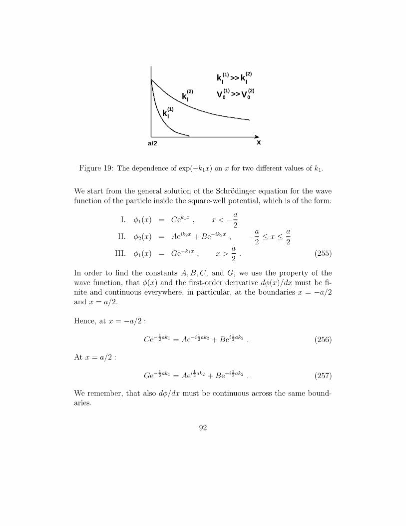
x

k

k

I

I(1)

(2)

kI(1) >> kI

(2)

V0(1) >> V0

(2)

a/2

Figure 19: The dependence of exp(−k1x) on x for two different values of k1.

We start from the general solution of the Schrodinger equation for the wavefunction of the particle inside the square-well potential, which is of the form:

I. φ1(x) = Cek1x , x < −a2

II. φ2(x) = Aeik2x +Be−ik2x , −a2≤ x ≤ a

2

III. φ1(x) = Ge−k1x , x >a

2. (255)

In order to find the constants A,B,C, and G, we use the property of thewave function, that φ(x) and the first-order derivative dφ(x)/dx must be fi-nite and continuous everywhere, in particular, at the boundaries x = −a/2and x = a/2.

Hence, at x = −a/2 :

Ce−1

2ak1 = Ae−i 1

2ak2 +Bei 1

2ak2 . (256)

At x = a/2 :

Ge−1

2ak1 = Aei 1

2ak2 +Be−i 1

2ak2 . (257)

We remember, that also dφ/dx must be continuous across the same bound-aries.

92

Since

I.dφ1

dx= Ck1e

k1x ,

II.dφ2

dx= iAk2e

ik2x − iBk2e−ik2x ,

III.dφ1

dx= −Gk1e

−k1x , (258)

we find that at x = −a/2:

Ck1e− 1

2ak1 = ik2

(

Ae−1

2iak2 − Be

1

2iak2

)

, (259)

and at x = a/2:

−Gk1e− 1

2ak1 = ik2

(

Ae1

2iak2 − Be−

1

2iak2

)

. (260)

Dividing both sides of Eq. (259) by k1, we obtain

Ce−1

2ak1 = iβ

(

Ae−1

2iak2 −Be

1

2iak2

)

, (261)

where β = k2/k1.Comparing Eqs. (256) and (261), we get

Ae−i 1

2ak2 +Bei 1

2ak2 = iβ

(

Ae−1

2iak2 −Be

1

2iak2

)

, (262)


A =(iβ + 1)

(iβ − 1)Beiak2 . (263)

Hence, substituting Eq. (263) into Eq. (256), we find that

C =2iβ

(iβ − 1)Be

1

2ak1(iβ+1) . (264)

Since B 6= 0, as the particle exists inside the well, we have that C 6= 0indicating that there is a non-zero probability of finding the particle in theregion I. The probability is given by |φ1(x)|2, that is

|φ1(x)|2 = |C|2e−2k1|x| , (265)

93

where |x| = −x for x < 0. Thus,

|φ1(x)|2 = |B|2 4β2

(β2 + 1)e−2k1(|x|−a

2) . (266)

The probability is different from zero and decreases exponentially with therate 2k1. The constant |B| is found from the normalization of φ(x).

Exercise:

Show that the particle probability current density ~J is zero in region I, anddeduce that R = 1, T = 0. This is the case of total reflection, the particlecoming towards the barrier will eventually be found moving back. ”Eventu-ally”, because the reversal of direction is not sudden. Quantum barriers are”spongy” in the sense the quantum particle may penetrate them in a waythat classical particles may not.

Consider now the continuity conditions at x = a/2. From the symmetryof the system, we expect that the constant G, similar to C, will be differ-ent from zero, and may be found in a similar way as we have found theconstant C.

From Eqs. (257) and (260), and using Eq. (263), we find two solutions forthe constant G in terms of B:

Ge−1

2ak1 = B

(

ue3

2iak2 + e−

1

2iak2

)

, (267)

Ge−1

2ak1 = −iβB

(

ue3

2iak2 − e−

1

2iak2

)

, (268)

where

u =(iβ + 1)

(iβ − 1). (269)

Here, we have two solutions for G. However, we cannot accept both of thesolutions as it would mean that there are two different probabilities of findingthe particle at a point x inside the region III. Therefore, we have to find underwhich circumstances these two solutions are equal.

Dividing Eq. (268) by (267), we obtain

iβ(

ue2iak2 − 1)

(ue2iak2 + 1)= −1 , (270)

94

from which we find that the solutions (267) and (268) are equal when

tan(ak2) =2k1k2

k22 − k2

1

. (271)

To proceed further, we introduce dimensionless parameters

ε =1

2ak2 =

1

2a

√

(

2mE

h2

)2

, (272)

√

ξ2 − ε2 =1

2ak1 , (273)

where

ξ2 =(

1

2a2mV0

h

)2

. (274)

We see from the relation ε = 12ak2 that determining ε we can get the

energy E of the particle inside the well. In order to show this, we rewriteEq. (271) in terms of ε and ξ, and find

ε tan ε =√

ξ2 − ε2 . (275)

This is a transcendental equation which, can be solved graphically as follows.Introducing the notation

p(ε) = ε tan ε ,

q(ε) =√

ξ2 − ε2 , (276)

we find solutions of the equation p(ε) = q(ε) by plotting separately p(ε) andq(ε). The functions p(ε) and q(ε) are shown in Fig. 20. The intersectionpoints of the two curves gives the solutions of the equation p(ε) = q(ε). Wesee from the figure that the equation p(ε) = q(ε) is satisfied only for discrete(finite) values of ε. Since the energy E is proportional to ε, see Eq. (272),we find that the energy of the particle is quantized in the region II, i.e. theenergy spectrum is discrete.

The number of solutions, which will give us the number of energy levels,depends on ξ, but always is finite. We see from Fig. 20 that there we have

one solution for ξ < π ,

two solutions for ξ < 2π ,

three solutions for ξ < 3π ,

95

.p( ) p( )

q( )

π 2ππ0 3π2 2

ε

ε ε

ε

p( )ε

ε = ξ

Figure 20: p(ε) and q(ε) as a function of ε.

and so on. The number of solutions determines the number of energy levelsinside the well.

We remember that

ξ2 =1

4a2(

k21 + k2

2

)

=ma2V0

2h2 . (277)

Thus, ξ is determined by the dimensions of the well.

96

Example:

Consider a potential well with ξ = 4. Since ξ < 2π, we see from Fig. 20that in this case there are two solutions for ε: ε1 = 1.25 and ε2 = 3.60.

Once we have the allowed values of ε, we can find the allowed values ofthe energy E. Since

ε =1

2ak2 ,

√

ξ2 − ε2 =1

2ak1 , (278)

and

k1 =

√

2m

h2 (V0 − E) , k2 =

√

2m

h2 E , (279)

we get

√ξ2 − ε2

ε=k1

k2=

√

V0 − E

E, (280)

from which we find

E =ε2

ξ2V0 . (281)

Hence, for ε1 = 1.25 and ε2 = 3.60, we get E1 = 0.098V0 and E2 = 0.81V0,respectively.

V0E

E 1

2

Figure 21: Energy levels inside the well with ξ = 4.

97

Exercise at home:

A rectangular potential well is bounded by a wall of infinite high on oneside and a wall of high V0 on the other, as shown in Fig. 22. The well has awidth a and a particle located inside the well has energy E < V0.

(a) Find the wave function of the particle inside the well.

V 0

0 a xregion IIIregion

Figure 22: Potential well of semi-infinite depth.

(b) Show that the energy of the particle is quantized.

(c) Discuss the dependence of the number of energy levels inside the wellon V0.

98

8.3 Quantum tunneling

When the potential barrier has a finite width, the tunneling effect can appear,that the particle with energy E < V0 can not only penetrate the barrier, it caneven pass through the barrier and appear on the other side. This phenomenonis known as quantum tunneling. This effect depends on the relation betweenV0 and E and also on the thickness of the barrier (see Fig. 23).

VI II III

0

x

Figure 23: Tunneling effect through a potential barrier of a thickness a.

How can we understand this process of a particle tunneling through aseemingly impenetrable barrier? How large is the probability that the particlepasses through the barrier? To answer these questions, we can use a wavepicture of the particle. We have already learnt that the particle wave functiondoes not terminate abruptly at the edge of the barrier, but actually leaks outthe barrier.

Let us perform the detailed calculations of the tunneling probability.

Rigorous calculations:

Consider a particle moving from the left and acting on the rectangular po-tential barrier, Fig. 23. Assume that E < V0. The solution of the Schrodingerequation for the three regions is

I. φ1(x) = Aeik1x +Be−ik1x , x < −a2

II. φ2(x) = Ce−k2x +Dek2x , −a2≤ x ≤ a

2

III. φ1(x) = F eik1x +Ge−ik1x , x >a

2(282)

99

where k1 =√

2mE/h and k2 =√

2m(V0 − E)/h.The continuity conditions for the wave function and the first-order deriva-

tive at x = −a/2 are

Ae−ik1a2 +Beik1

a2 = Cek2

a2 +De−k2

a2 ,

Ae−ik1a2 − Beik1

a2 =

ik2

k1

(

Cek2a2 −De−k2

a2

)

. (283)

The continuity conditions at x = a/2 are

Ce−k2a2 +Dek2

a2 = F eik1

a2 +Ge−ik1

a2 ,

−Ce−k2a2 +Dek2

a2 =

ik1

k2

(

F eik1a2 −Ge−ik1

a2

)

. (284)

The continuity conditions (283) and (284) can be written in matrix forms as(

AB

)

=1

2

(

1 + ik2

k1

)

ek2a2+ik1

a2

(

1 − ik2

k1

)

e−k2a2+ik1

a2

(

1 − ik2

k1

)

ek2a2−ik1

a2

(

1 + ik2

k1

)

e−k2a2−ik1

a2

(

CD

)

, (285)

and(

CD

)

=1

2

(

1 − ik1

k2

)

ek2a2+ik1

a2

(

1 + ik1

k2

)

ek2a2−ik1

a2

(

1 + ik1

k2

)

e−k2a2+ik1

a2

(

1 − ik1

k2

)

e−k2a2−ik1

a2

(

FG

)

. (286)

The relationship between the solution on the left of the barrier and thesolution on the right can now be obtained by substituting the matrix equation(286) into the right hand side of the matrix equation (285), and then weobtain

(

AB

)

=

(

cosh k2a+ iε2

sinh k2a)

eik1a iη2

sinh k2a

− iη2

sinh k2a(

cosh k2a− iε2

sinh k2a)

e−ik1a

(

FG

)

(287)

with ε = k2

k1− k1

k2and η = k2

k1+ k1

k2. The solution with G = 0 is of particular

interest as it represents the situation where no particles are incident on thebarrier from the right. In this case

F

A=

e−ik1a

cosh(k2a) + 12iε sinh(k2a)

. (288)

100

Hence, the transmission coefficient of the particle current is

T =|F |2|A|2 =

[

cosh2(k2a) +(

ε

2

)2

sinh2(k2a)

]−1

=

[

1 +

(

(

ε

2

)2

+ 1

)

sinh2(k2a)

]−1

=

[

1 +V 2

0 sinh2(k2a)

4E(V0 − E)

]−1

. (289)

When E > V0, the solution changes only in the region II, and the newsolution can be obtained from the old solution by replacing k2 by ik′2, where

k′2 =√

2m(E − V0)/h. So that the expression for T changes to

T =

[

1 +V 2

0 sin2(k′2a)

4E(E − V0)

]−1

. (290)

First, note that if there is no barrier, V0 = 0, and then there is 100% trans-mission. Thus, there is nothing particularly remarkable about the solutionwhen V0 = 0. Its physical interest lies in what happens when V0 6= 0.

For V0 6= 0, one could expect from the classical mechanics that T = 0 forE < V0, and T = 1 for E > V0. However, Eq. (289) shows that T is notzero for E < V0 (non-zero transmission), and Eq. (290) shows that T < 1 forE > V0 (non-zero reflection).

Thus, tunneling effect for E < V0 and partial reflection at the barrierfor E > V0 are quantum phenomena. In the classical limit of h → 0, theparameter k2 → ∞, and then T → 0. Hence, in the classical limit, there is nopossibility of the particle of an energy E < V0 to pass the barrier. Moreover,since that k2 is proportional to mass of the particle, the transmission coeffi-cient (289) is large for light particles and decreases with the increasing m.

There is the further interesting phenomenon for the case of E > V0. Onecan see from Eq. (290) that if k′2a = nπ, n = 1, 2, 3, . . ., there is 100% trans-mission from region I to III. This phenomenon is analogous to the behaviorof coated lenses in optics. Otherwise, quantum effect (partial reflection) ap-pears.

101

Quantum tunneling is important in the understanding of number of phys-ical phenomena such as thermonuclear reactions and conduction in metalsand semiconductors. In 1928, Gamov, Condon and Gurney used quantumtunneling to explain the α-decay of unstable nuclei, in which an alpha particle(a helium nucleus) is emitted from a radioactive nucleus. The alpha particlehas energy which is less than the high of the potential barrier keeping theparticle inside the nucleus. Nevertheless, alpha particles tunnel through thebarrier and are detected outside the nucleus.

Tunneling has also been used in a number of electronic devices. One is atunnel diode in which the current of electrons is controlled by adjusting theenergy E of the electrons. This changes the value of k2 and thus the rate theelectrons tunnel through the device.

The most advanced application of quantum tunneling is the scanningtunneling microscope. A probe needle is held very close (< 1 nm) above aconducting object and scanned across it. The object is at a positive volt-age V with respect to the probe needle. However, for electrons to pass fromthe needle to the object, they have to overcome the work function of theneedle material. This creates a potential barrier through which electrons cantunnel. As they tunnel through the potential barrier they generate a currentwhose the variation tells us about the distance between the needle and theobject.

Challenging problem: Quantum tunneling from and into a semi-finite well

In the problem discussed in lecture, we have shown there are no restrictionson the energy of a particle to tunnel through the barrier. The explanation ofthis effect is simple: The particle of an arbitrary energy can tunnel throughthe barrier because there are no restrictions on energies which the particlecan have in the region III. Lets us consider the exercise from page 98, arectangular potential well of width a bounded by a wall of infinite high onone side and a barrier of high V0 and infinite thickness on the other. Wehave learnt that inside the well, region I, a particle can have only a limitednumber of discrete energies.

102

V 0

x0 a 2aII

E

region I region region III

Figure 24: Potential well of semi-infinite depth limited by a barrier of high V0

and width a.

(a) Now imagine what happens if the thickness of the barrier (region II)is finite and the particle of energy E < V0 is inside the potential well. Doyou expect the energy levels of the particle in region I are still discrete?

(b) Suppose that the particle of energy E < V0 is in the region III onthe right of the barrier and moves towards the barrier, as shown in Fig. 24.Find the tunneling coefficient and determine whether for each E, in the range0 < E < V0, the particle can tunnel to the region I, i.e. determine whetherthe energy spectrum in the region I is discrete or continuous. Would youexpect this result without the detailed calculations?

103

9 Multi-Dimensional Quantum Wells:

Quantum Wires and Quantum Dots

We have seen that in the one-dimensional case, particles confined into asmall region can have quantized energies, can be be found in ”classicallyforbidden” region and even can tunnel through this region. Although theone-dimensional case is very useful in the illustration and understanding ofthe quantum effects, we need a full three-dimensional treatment if we wantto illustrate applications of quantum mechanics to atoms, solid state, andnuclear physics. The application to atoms will be discussed in a separatelecture on Angular Momentum and Hydrogen Atom, Chapter 15. In thislecture, we extend the concept of quantum wells from one to three dimensions.

��

��

��

�� x

y

z

a

a

L

Figure 25: A three dimensional well of sides x = a, y = a, and z = L. Inside the

well V = 0. The potential is infinite at the xy walls and can be set zero at the z

walls (quantum wire), or infinite (quantum dot).

We can picture a quantum wire as a pipe, shown in Fig. 25, and particlesmoving freely along this pipe, just like cars driving through a mountain tun-nel. However, we must be careful when using analogies to describe quantum

104

phenomena. We expect the cars to drive along the bottom of the tunnel, butwe would be surprised to see the cars driving through mid-air a few metersabove the tunnel floor. This is precisely how the particles appear to behavein a quantum wire.

9.1 General solution of the three-dimensionalSchrodinger equation

Let us find the wave function of a particle located inside the well and itsenergies. The wave function and the energies are found from the three-dimensional Schrodinger equation

− h2

2m∇2Ψ + VΨ = E . (291)

We see that in cartesian coordinates ∂2/∂x2 in the one-dimensional case isreplaced in three dimensions by the Laplacian

∇2 =∂2

∂x2+

∂2

∂y2+

∂2

∂z2. (292)

Since x, y, z are independent (separable) variables, the wave function is alsoseparable into three independent functions Ψx, Ψy, and Ψz. In this case, wecan find the solution of the Schrodinger equation in product form

Ψ(x, y, z) = Ψx(x)Ψy(y)Ψz(z) . (293)

Substituting this into the Schrodinger equation and dividing both sides byΨxΨyΨz, we obtain

− h2

2mΨx

d2Ψx

dx2− h2

2mΨy

d2Ψy

dy2− h2

2mΨz

d2Ψz

dz2= E , (294)

where, as before, we have put V = 0 inside the well, but outside the well wewill set V = ∞.

Since each term on the left-hand side of Eq. (294) is a function of only onevariable, each will be independent of any change in the other two variables.

105

Thus, Eq. (294) can be separated into three independent equations. Toillustrate this, we write this equation as

− h2

2mΨx

d2Ψx

dx2= E +

h2

2mΨy

d2Ψy

dy2+

h2

2mΨz

d2Ψz

dz2. (295)

The lhs involves all of the x dependence. If we change x any way we want, therhs is not affected. Thus, it must be that both sides are equal to a constant,say Ex:

− h2

2mΨx

d2Ψx

dx2= Ex , (296)

− h2

2mΨy

d2Ψy

dy2− h2

2mΨz

d2Ψz

dz2= E − Ex . (297)

Equation (297), that depends only on y and z variables can be written as

− h2

2mΨy

d2Ψy

dy2= E − Ex +

h2

2mΨz

d2Ψz

dz2. (298)

Again, both sides depend on different variables, the lhs depends only on yand the rhs depends only on z, thus both sides are equal to a constant,say Ey:

− h2

2mΨy

d2Ψy

dy2= Ey , (299)

− h2

2mΨz

d2Ψz

dz2= E − Ex − Ey . (300)

Hence, after the separation of the variables, one differential equation in threevariables has turned into three independent equations of one variable each

− h2

2mΨx

d2Ψx

dx2= Ex , (301)

− h2

2mΨy

d2Ψy

dy2= Ey , (302)

− h2

2mΨz

d2Ψz

dz2= Ez , (303)

106

where Ez = E − Ex − Ey.The wave function of the particle inside the well and its energies are

found from these three independent equations. The parameters Ex, Ey andEz are separation constants, and represent energies of motion along the threeCartesian axis x, y and z. It is easily to see that these three constants satisfythe equation

Ex + Ey + Ez = E . (304)

The solutions of the equations (301) and (302) are the same as that forthe infinite square well in one dimension, and are given by

Ψx = A sin(

n1π

ax)

, n1 = 1, 2, 3, . . . , (305)

Ψy = B sin(

n2π

ay)

, n2 = 1, 2, 3, . . . , (306)

with energies

Ex = n21

π2h2

2ma2and Ey = n2

2

π2h2

2ma2. (307)

9.2 Quantum wire and quantum dot

The solution for the z component of the motion, Eq. (303), depends onwhether the z sides of the well have zero or infinite potential. For zeropotential, the z direction is free for the motion of the particle (quantumwire), and is given by the wave function

Ψz = Ceikzz , (308)

where k2z = 2mEz/h

2, and Ez can have arbitrary values.If the potential at the z sides is infinite, we have an example of quantum

dot3. In this case, the solution of Eq. (303) is the same as for the x and ycomponents

Ψz = C sin(

n3π

Lz)

, n3 = 1, 2, 3, . . . , (309)

3It would be more correct to call the quantum dot a quantum box, but in many cal-culations, quantum dots that have spherical symmetries are approximated by rectangularboxes.

107

with the Ez energy taking only discrete values

Ez = n23

π2h2

2mL2. (310)

Thus, we can summarize that for a quantum wire, the wave functions ofthe particle are of the form

Ψn1,n2= D sin

(

n1π

ax)

sin(

n2π

ay)

eikzz , (311)

and the corresponding energies are given by

E =π2h2

2ma2

(

n21 + n2

2

)

+ Ez , with n1, n2 = 1, 2, 3, . . . , (312)

where D = ABC is a constant which is found from the normalization condi-tion of the wave function. It is easy to show that

D =2

a

√

2

L. (313)

The proof is left to the students.

Interesting observation:Since the energy of the particle in the y direction can never be zero, theparticle will never move at the floor of the wire. Because the motion of theparticle is restricted (quantized) in two dimensions, a quantum wire is some-times referred to as a one-dimensional system.

For a quantum dot with L = a, the wave functions of the particle insidethe well are of the form

Ψn1,n2,n3=(

2

a

)

3

2

sin(

n1π

ax)

sin(

n2π

ay)

sin(

n3π

az)

, (314)

and the corresponding energies are given by

E =π2h2

2ma2

(

n21 + n2

2 + n23

)

, with n1, n2, n3 = 1, 2, 3, . . . . (315)

108

Thus, energy of the particle in a quantum dot is quantized in all three di-rections. Because the motion of the particle is now restricted in all threedimensions (quantum confinement), a quantum dot is sometimes referred toas a zero-dimensional system. Quantum dots are also regarded as artificialatoms.

One can notice that the results obtained for the three-dimensional caseare similar to that obtained for the one-dimensional case. However, there isa significant difference between these two cases. For the three-dimensionalcase there might be few wave functions corresponding to the same energy.We can illustrate this on a simple example of energies and the correspondingwave functions of a quantum dot:The lowest energy state (the ground state), for which n1 = n2 = n3 = 1, hasenergy

E =3π2h2

2ma2, (316)

and there is only one wave function (singlet) corresponding to this energy.However, there are three wave functions corresponding to energy

E =6π2h2

2ma2, (317)

as there are three combinations of n1, n2 and n3 whose squares sum to 6.These combinations are n1 = 2, n2 = 1, n3 = 1, or n1 = 1, n2 = 2, n3 = 1, orn1 = 1, n2 = 1, n3 = 2. The three wave functions corresponding to this energyare Ψ2,1,1,Ψ1,2,1, and Ψ1,1,2. We say that the energy level is degenerate.

It is easy to see from Eq. (315) that the degeneracy of the energy levelsis characteristic of quantum wells whose the sides are of equal lengths. Thedegeneracy can be lifted, if the sides of the well were of unequal lengths.

Exercise at home:

Find the number of wave functions (energy states) of a particle in a quantumwell of the sides of equal lengths corresponding to energy

E =9π2h2

2ma2,

i.e. for the combination of n1, n2 and n3 whose squares sum to 9.

109

10 Linear Operators and Their Algebra

We have seen that in quantum physics energy and momentum appear asmathematical operations, which we call operators. We now extend the ideaof operators into arbitrary quantities, and postulate that any quantity inquantum physics is specified by a linear operator.

An operator A is linear if for arbitrary functions fi and gi, and arbitrarycomplex numbers ci, such that

Af1 = g1 and Af2 = g2 ,

the linear superposition is

A (c1f1 + c2f2) = c1Af1 + c2Af2 = c1g1 + c2g2 . (318)

10.1 Algebra of operators

The sum of two operators A and B and their product are defined as(

A+ B)

f = Af + Bf , (319)(

AB)

f = A(

Bf)

. (320)

The operators obey the following algebraic rules:

1. A+ B = B + A ,

2. A+ B + C =(

A+ B)

+ C = A+(

B + C)

,

3. ABC = A(

BC)

=(

AB)

C ,

4.(

A+ B)

C = AC + BC . (321)

The power of an operator and the sum of two operators is defined as

1. A2 = AA , A3 = AAA , etc.

2.(

A+ B)2

=(

A + B) (

A + B)

= A2 + B2 + AB + BA . (322)

In general, AB 6= BA. Thus, multiplication of operators is not necessarilycommutative.

110

We can define a commutator:[

A, B]

= AB − BA , (323)

and say, that two operators commute if[

A, B]

= 0 . (324)

We can also define anticommutator as{

A, B}

≡[

A, B]

+= AB + BA , (325)

and we say that two operators anticommute if[

A, B]

+= 0 . (326)

Inverse operator:

The inverse of an operator A, if it exists, is defined by

AA−1 = A−1A = 1 , (327)

where 1 is the unit operator defined by

1f = f . (328)

Hermitian adjoint: (Hermitian conjugate)

Operator A† is the Hermitian adjoint of an operator A if for twofunctions f and g that vanish at infinity

∫

f ∗AgdV =∫

(

A†f)∗gdV . (329)

Properties of Hermitian conjugate:

1.(

A†)†

= A . (330)

111

Proof:∫

f ∗AgdV =∫

(

A†f)∗gdV =

∫

g(

A†f)∗dV =

(∫

g∗A†fdV)∗

=(∫ (

(

A†)†g)∗fdV

)∗=∫ (

(

A†)†g)

f ∗dV

=∫

f ∗(

(

A†)†g)

dV , (331)

as required♦.

2.(

AB)†

= B†A† . (332)

Proof:∫

f ∗(

AB)†gdV =

∫

(

ABf)∗gdV =

∫

[

A(

Bf)]∗

gdV . (333)

Introducing the notation Bf = u, we get

∫

(

Au)∗gdV =

∫

u∗A†gdV =∫

(

Bf)∗A†gdV

=∫

f ∗B†A†gdV . (334)

Thus,(

AB)†

= B†A†,

as required♦.

112

10.2 Hermitian operators

Operator A is called Hermitian if

A† = A , (335)

i.e. when∫

f ∗AgdV =∫

(

Af)∗gdV . (336)

10.2.1 Properties of Hermitian operators

If A and B are Hermitian then:

1. A + B is Hermitian,

2. A2, A3, etc. are Hermitian,

3. cA is Hermitian if c is a real number.

Proof of the property 3:∫

f ∗(

cA)

gdV =∫

(

cAf)∗gdV = c∗

∫

(

Af)∗gdV , (337)

as required♦.

4. AB is Hermitian only if A and B commute.

Proof:(

AB)†

= B†A† = BA . (338)

Hence,(

AB)† 6= AB unless A and B commute,

as required♦.

113

5. From the property 4, we have that the commutator[

A, B]

is not Hermi-

tian, even if A and B are Hermitian.

Proof:[

A, B]†

=(

AB − BA)†

=(

AB)† −

(

BA)†

= B†A† − A†B† = BA− AB = −[

A, B]

, (339)

as required♦.

6. However, i[

A, B]

is Hermitian.

Proof is left for the students.

7. For an arbitrary operatorA, the product AA† is Hermitian.

Proof:(

AA†)†

=(

A†)†A† = AA† , (340)

as required♦.

8. If A is non-Hermitian, A + A† and i(

A− A†)

are Hermitian. Hence,

A can be written as a linear combination of two Hermitian operators

A =1

2

(

A + A†)

+1

2i

(

i(

A− A†))

. (341)

10.2.2 Examples of Hermitian operators

1. Position operator ~r is Hermitian.

Since |~r| is a real number and ~rg is just a multiplication of the functiong by ~r, we have

∫

f ∗~rgdV =∫

~rf ∗gdV =∫

(

~rf)∗gdV . (342)

114

2. Potential V (~r).

Since ~r is Hermitian, an arbitrary function of ~r is also Hermitian.

3. Momentum operator is Hermitian.

Proof:

∫

V

(

~pf)∗gdV =

∫

V

(

h

i∇f

)∗gdV = − h

i

∫

V(∇f ∗) gdV

= − hi

∫

V∇ (f ∗g) dV +

h

i

∫

Vf ∗ (∇g) dV

= − hi

∫

V∇ (f ∗g) dV +

∫

Vf ∗(

h

i∇g

)

dV . (343)

Using the Gauss’s divergence theorem, we get that Eq. (343) can be writtenas

= − hi

∮

Sf ∗gdS +

∫

Vf ∗(

~pg)

dV . (344)

First integral in Eq. (344) vanishes as f and g vanish at infinity, and thereforewe get

∫

V

(

~pf)∗gdV =

∫

Vf ∗(

~pg)

dV , (345)

which means that ~p is Hermitian,

as required♦.

We have defined before the eigenvalues and eigenfunctions of the Hamilto-nian of a particle, see Section 7.3. The idea of eigenvalues and eigenfunctionscan be extended to arbitrary operators. Thus, we can state:

If AΨ = αΨ, then Ψ is an eigenfunction of A with eigenvalue α.

115

Example:

Determine if the function Ψ = e2x is an eigenfunction of the operators (a)A = d/dx, (b) B = ()2, and (c) C =

∫

dx.

(a) Operating on the wave function Ψ with the operator A, we obtain

AΨ =d

dxe2x = 2e2x = 2Ψ , (346)

which is a constant times the original function. Therefore, Ψ = e2x is aneigenfunction of the operator A = d/dx with an eigenvalue α = 2.

I leave the solution of the parts (b) and (c) to the students.

Hermitian operators play the important role in quantum mechanics as theyrepresent physical quantities. This importance arises from the fact thateigenvalues of an Hermitian operator are real.

Proof:

Assume that α is an eigenvalue of an Hermitian operator A correspondingto the eigenfunction f (that vanishes at infinity). Then

α = α∫

V|f |2dV =

∫

Vf ∗αfdV =

∫

Vf ∗AfdV

∫

V

(

Af)∗fdV =

∫

Vα∗f ∗fdV = α∗

∫

V|f |2dV = α∗ , (347)

as required♦.

116

10.3 Scalar product and orthogonality of two eigen-functions

Two functions Ψ1(~r) and Ψ2(~r) are orthogonal if

∫ +∞

−∞Ψ∗

1(~r)Ψ2(~r)dV = 0 . (348)

The orthogonality of two functions is related to the orthogonality of twovectors. The vectors are orthogonal when the scalar product of the vectorsis zero. In analogy, we can write a scalar product of two functions as

(Ψi,Ψj) =∫

Ψ∗i (~r)Ψj(~r)dV = ajδij , (349)

where aj is a positive constant and δij is the Kronecker delta function.

When aj = 1, we say that the functions are orthonormal.

The complex functions Ψi form a complex linear vector space. The infinite-dimensional vector space of orthonormal functions is called Hilbert space.

The scalar product

(Ψi,Ψi) = ||Ψi|| =∫

|Ψi|2 dV , (350)

where Ψi is a square integrable function, is called the norm of the state (vec-tor) Ψ. For a state function that represents physical quantity the norm isfinite. If the functions are orthonormal, the norm ||Ψi|| = 1.

Example of orthogonal functions:

Examples of orthogonal functions are sines and cosines functions. Theirproduct with any other function of the same class gives zero when integratedover all ranges of variable, unless the two multiplied functions are identical.

∫ 2π

0sin(mφ) sin(nφ) dφ =

{

0 for m 6= nπ for m = n

(351)

117

∫ 2π

0cos(mφ) cos(nφ) dφ =

{


(352)

∫ 2π

0sin(mφ) cos(nφ) dφ = 0 for all m and n . (353)

From the orthogonality of the sines functions, we see that the eigenfunc-tions of a particle in an infinite square well potential, Eq. (242), correspondingto different energies (n 6= m) are orthogonal.

Having available the definition of orthogonal functions, we can formulatean important property of eigenfunctions of a linear Hermitian operator.

Eigenfunctions of a linear Hermitian operator belonging to dif-ferent eigenvalues are orthogonal.

Proof:

Consider a Hermitian operator A. Let f and g are two eigenfunctions ofA corresponding to two different eigenvalues αf and αg, respectively,

Af = αff ,

Ag = αgg , (354)

where αf , αg are real numbers.

Since(

Af)∗

= αff∗, we can write

∫

(

Af)∗gdV −

∫

f ∗(

Ag)

dV = (αf − αg)∫

f ∗gdV . (355)

However∫

(

Af)∗gdV =

∫

f ∗(

Ag)

dV , (356)

and therefore the lhs of Eq. (355) vanishes. Since, αf 6= αg, we have

(f, g) =∫

f ∗gdV = 0 , (357)

as required♦.

118

10.4 Expectation value of an operator

In classical physics, an expectation or average or mean value of an arbitraryquantity A is obtained by weighting each measured value Ai by the associatedprobability Pi and summing over all the measurements N . Thus,

〈A〉 =∑

i

PiAi i = 1, 2, . . . , N , (358)

where Pi is a probability of measuring the value Ai.

How do we calculate expectation values in quantum physics?

Consider an operator A acting on a function Ψi. Suppose that AΨi exists,then the scalar product

(

Ψi, AΨi

)

=∫

Ψ∗i AΨidV (359)

is called the expectation or average or mean value of the operator A in thestate Ψi.

Similarly as in classical physics, the expectation value can be calculatedfrom the probability density as

〈A〉 =∫

Aρ(~r)dV =∫

A |Ψi|2 dV =∫

Ψ∗i AΨidV , (360)

where the order of the factors under the integral is not important.

Properties of the expectation value

1. Expectation value of a Hermitian operator is real.

Proof:

〈A〉 =∫

Ψ∗i AΨidV =

∫

(

AΨi

)∗ΨidV

=∫

Ψi

(

AΨi

)∗dV =

(∫

Ψ∗i AΨidV

)∗= 〈A〉∗ , (361)

as required♦.

119

2. Expectation value of an arbitrary operator B satisfies the following equa-tion of motion

d

dt〈B〉 =

⟨

∂B

∂t

⟩

+i

h

⟨[

H, B]⟩

. (362)

Proof:

Since

〈B〉 =∫

Ψ∗i BΨidV ,

we have

d

dt〈B〉 =

∫

(

∂Ψ∗

∂t

)

BΨdV +∫

Ψ∗(

∂B

∂t

)

ΨdV +∫

Ψ∗B

(

∂Ψ

∂t

)

dV .

From the Schrodinger equation

ih∂Ψ

∂t= HΨ ,

and its complex conjugate

−ih∂Ψ∗

∂t= HΨ∗ ,

we obtain

d

dt〈B〉 =

⟨

∂B

∂t

⟩

+i

h

∫

HΨ∗BΨdV − i

h

∫

Ψ∗BHΨdV .

Since H is Hermitian, we finally get

d

dt〈B〉 =

⟨

∂B

∂t

⟩

+i

h

∫

Ψ∗(

HB − BH)

ΨdV

=

⟨

∂B

∂t

⟩

+i

h

⟨[

H, B]⟩

,

as required♦.

120

Thus, expectation value of the operator B can depend on time even if theoperator does not depend explicitly on time (∂B/∂t = 0).When [H, B] = 0, we have that d〈B〉/dt = 0, and then the expectation valueis constant in time. In analogy to classical physics, we call B a constant ofmotion.

We have already shown that expectation values of Hermitian operatorsare real. In term of the scalar product this is characterized by

(

Ψi, AΨi

)

=(

Ψi, AΨi

)∗. (363)

From this property, we have in general, that for Hermitian operators(

Ψi, AΨj

)

=(

Ψj, AΨi

)∗. (364)

Proof:(

Ψi, AΨj

)

=∫

Ψ∗i AΨjdV =

∫

(

AΨi

)∗ΨjdV =

∫

Ψj

(

AΨi

)∗dV

=(∫

Ψ∗jAΨidV

)∗=(

Ψj, AΨi

)∗,

as required♦.

The properties (363) and (364) is very often used to check whether oper-ators are Hermitian.

Example:

Consider two operators A = d/dx and B = d2/dx2 acting on two orthonor-mal wave functions Ψ1 = a sin(nx) and Ψ2 = a cos(nx), where n is a realnumber, a = 1/

√π and x ∈ 〈−π, π〉.

Are the operators A and B Hermitian?

Solution:

First, consider the operator A = d/dx. Since

AΨ1 = ad

dxsin(nx) = an cos(nx) = anΨ2 , (365)

121

and

AΨ2 = ad

dxcos(nx) = −an sin(nx) = −anΨ1 , (366)

we find the following values of the scalar products(

Ψ1, AΨ1

)

= −an (Ψ1,Ψ2) = 0 ,(

Ψ1, AΨ2

)

= −an (Ψ1,Ψ1) = −an ,(

Ψ2, AΨ2

)

= −an (Ψ2,Ψ1) = 0 ,(

Ψ2, AΨ1

)

= an (Ψ2,Ψ2) = an . (367)

Hence(

Ψ1, AΨ1

)

=(

Ψ2, AΨ2

)∗, (368)

but(

Ψ1, AΨ2

)

= −an 6=(

Ψ2, AΨ1

)∗= an . (369)

Thus, the operator A = d/dx is not Hermitian.

Consider now the operator B = d2/dx2. Since

BΨ1 = ad2

dx2sin(nx) = −an2 sin(nx) = −an2Ψ1 , (370)

and

BΨ2 = ad2

dx2cos(nx) = −an2 cos(nx) = −an2Ψ2 , (371)

we find the following values of scalar products(

Ψ1, BΨ1

)

= −an2 (Ψ1,Ψ1) = −an2 ,(

Ψ1, BΨ2

)

= −an2 (Ψ1,Ψ2) = 0 ,(

Ψ2, BΨ2

)

= −an2 (Ψ2,Ψ2) = −an2 ,(

Ψ2, BΨ1

)

= −an2 (Ψ2,Ψ1) = 0 . (372)

122

Hence(

Ψ1, BΨ1

)

= −an2 =(

Ψ2, BΨ2

)∗, (373)

and(

Ψ1, BΨ2

)

= 0 =(

Ψ2, BΨ1

)∗. (374)

Thus, the operator B = d2/dx2 is Hermitian.

Exercise at home:

Prove, using the condition (364) and the wave functions Ψ1 and Ψ2 of theabove example, that the momentum operator px = −ih∂/∂x is Hermitian.

123

10.5 The Heisenberg uncertainty principle revisited

In Section 6.6, we have shown that the uncertainties in the position andmomentum of a particle satisfy the relation

∆y∆py = h . (375)

This relation says the position and momentum of a particle cannot be mea-sured simultaneously with the same precision. This is known as the Heisen-berg uncertainty relation, or the Heisenberg uncertainty principle, andwe will show that the relation is a direct consequence of the noncommutivityof the position and momentum operators

[y, py] = ih . (376)

In fact, the Heisenberg uncertainty relation can be formulated for arbitrarytwo Hermitian operators that do not commute. In other words, if A and Bare two Hermitian operators that do not commute, the physical quantitiesrepresented by the operators cannot be measured simultaneously with thesame precision.

Theorem:

The variances 〈(∆A)2〉 = 〈A2〉 − 〈A〉2 and 〈(∆B)2〉 = 〈A2〉 − 〈A〉2 of twoHermitian operators satisfy the inequality

〈(∆A)2〉〈(∆B)2〉 ≥ −1

4〈[A, B]〉2 , (377)

which is called the Heisenberg inequality.

Proof:

First, we prove that for an arbitrary operator A the following inequalityholds

〈AA†〉 ≥ 0 . (378)

124

It is easy to prove the above inequality using the definition of the expectationvalue

〈AA†〉 =∫

Ψ∗AA†ΨdV =∫

(

A†Ψ)∗A†ΨdV =

∫

∣

∣

∣A†Ψ∣

∣

∣

2dV ≥ 0 . (379)

Now, we prove that for two Hermitian operators the following inequalityis satisfied

〈A2〉〈B2〉 ≥ −1

4〈[A, B]〉2 . (380)

To prove it, we introduce an operator

D = A+ izB , (381)

where z is an arbitrary real number.Hence, from Eq. (378), we find

〈DD†〉 = 〈(A+ izB)(A− izB)〉= 〈A2〉 − iz(〈AB − BA〉) + z2〈B2〉 ≥ 0 . (382)

This inequality is satisfied when

−〈AB − BA〉2 − 4〈A2〉〈B2〉 ≤ 0 . (383)

Hence

〈A2〉〈B2〉 ≥ −1

4〈[A, B]〉2 , (384)

as required.

Finally, since

[∆A,∆B] = [A, B] , (385)

where ∆U = U −〈U〉, (U = A, B), and replacing in Eq. (384), A→ ∆A andB → ∆B, we obtain the required Heisenberg uncertainty relation (377),as required♦.

125

Example 1. The Heisenberg uncertainty relation for the position and mo-mentum operators.

Since

[x, px] = ih , (386)

we obtain by substituting into Eq. (377), A = x and B = px

〈(∆x)2〉〈(∆px)2〉 ≥ 1

4h2 , (387)

or in terms of the standard deviations (fluctuations)

δxδpx ≥ 1

2h , (388)

where δx =√

〈(∆x)2〉 and δpx =√

〈(∆px)2〉.Similarly, we can show that for the y and z components of the position

and momentum

δyδpy ≥ 1

2h and δzδpz ≥ 1

2h . (389)

Note that the relation (375) satisfies the Heisenberg inequality as h > h/2.

Example 2. The Heisenberg uncertainty relation for the components ofthe electron spin.

Since

[σx, σy] = 2iσz , (390)

(For a poof, see Tutorial Set 8), where σx, σy, σz are the operators corre-sponding to the three components of the electron spin, we obtain

〈(∆σx)2〉〈(∆σy)

2〉 ≥ 〈σz〉2 , (391)

or

δσxδσy ≥ |〈σz〉| . (392)

The uncertainty relation (392) shows that the components of the electronspin cannot be measured simultaneously with the same precision.

126

10.6 Expansion of wave functions in the basis of or-thonormal functions

We now consider the most important property of orthonormal functions,which similar to the orthogonality, arises from the properties of vectors.

To illustrate this connection, consider a simple example:

In the Cartesian coordinates an arbitrary vector ~A can be written as a linearcombination of the orthonormal unit vectors

~A = (~i · ~A)~i+ (~j · ~A)~j + (~k · ~A)~k , (393)

where ~i, ~j and ~k are unit vectors in the directions x, y and z, respectively.

Proof:

We know from the vector analysis that in the Cartesian coordinates an ar-bitrary vector ~A may be presented in terms of components Ax, Ay, Az, andthree unit vectors oriented in the directions of the coordinate axis

~A = Ax~i + Ay

~j + Az~k . (394)

Since the components are the projections of the vector ~A on the coordinateaxis

Ax =~i · ~A , Ay = ~j · ~A , Az = ~k · ~A , (395)

we find that the vector (394) can be written in the form

~A = (~i · ~A)~i+ (~j · ~A)~j + (~k · ~A)~k , (396)

as required♦.

We can extend this property to n dimensional space and state that an ar-bitrary vector ~A can be written as a linear combination of thecoordinate (basis) unit vectors ~e as

~A =(

~e1 · ~A)

~e1 +(

~e2 · ~A)

~e2 + . . .+(

~en · ~A)

~en =m∑

n=1

(

~en · ~A)

~en , (397)

127

where(

~en · ~A)

is the scalar product of ~en and ~A, (nth component of ~A),

and ~ei · ~ej = δij.

The norm (magnitude) of the vector ~A is

|| ~A||2 = | ~A| =∑

n

(

~en · ~A)2

. (398)

Thus, we see that an arbitrary vector can be expressed as a linear combina-tion of the orthonormal vectors ~en.

In analogy, an arbitrary wave function Ψ can be expanded in termsof orthonormal wave functions Ψn as

Ψ =∑

n

cnΨn , (399)

(discrete spectrum of Ψn), or in the case of a continuous spectrum of Ψn

Ψ(~r) =∫

cn(~r)Ψn(~r)dVn , (400)

where cn are arbitrary (unknown) expansion coefficients, and dVn is the vol-ume element of the space the orthonormal functions Ψn(~r) are spanned.

We can find the coefficients cn(~r) by multiplying Eq. (400) by Ψ∗m(~r) and

integrating over all space as follows∫

Ψ∗m(~r)Ψ(~r)dV =

∫

cn(~r)∫

Ψ∗m(~r)Ψn(~r)dV dVn = cm(~r) , (401)

where we have used the orthonormality property of the Ψn functions∫

Ψ∗m(~r)Ψn(~r)dVn = δnm . (402)

In general, the coefficients cm(~r) are complex numbers and are called thecomponents of the function Ψ in the basis of the orthonormal functions Ψm.The components determine the function completely, and very often the co-efficients cm(~r) are called a representation of the wave function Ψ in thebasis Ψm.

The coefficients cm(~r) satisfy the following relation∫

V|cm(~r)|2 dV = 1 . (403)

128

Proof:

Multiplying Eq. (400) by Ψ∗(~r) and integrating over V , we obtain

∫

VΨ∗(~r)Ψ(~r)dV =

∫

V|Ψ(~r)|2 dV

=∫

V

∫

Vn

∫

Vm

c∗m(~r)cn(~r)ΨnΨmdVndVmdV

=∫

V

∫

Vn

c∗m(~r)cn(~r)δmndVndV =∫

V|cm(~r)|2 dV . (404)

Since,∫

V |Ψ|2dV = 1, we get∫

V |cm(~r)|2 dV = 1,as required♦.

From Eqs. (400) and (403), we see that |cm(~r)|2 can be interpreted asthe probability that a system, described by the wave function Ψ(~r), is in thestate described by the wave function Ψm(~r).

Example:

Let A is an operator and Ψ(~r) is an unknown wave function that is notan eigenfunction of A. Suppose, that we cannot find the explicit form ofΨ(~r) because we cannot solve the Schrodinger equation for Ψ(~r). However,we can find a form of the wave function in the basis of the eigenfunctions ofA. If Ψm(~r) is an eigenfunction of A, then

Ψ(~r) =∫

cm(~r)Ψm(~r)dVm . (405)

129

11 Dirac Notation

Dirac introduced a very useful (compact) notation of state vectors (wavefunctions) Ψi in terms of ”bra” 〈i| and ”ket” |i〉 vectors.

For example, a wave function Ψi can be expressed by a ket vector |Ψi〉,and Ψ∗

i by a bra vector 〈Ψi|. This notation can be further simplified to |i〉and 〈i|, respectively.

Let us illustrate what kind of simplifications we will get using the Diracnotation.

In the Dirac notation, a scalar product is written as

(Ψi,Ψj) = 〈Ψi|Ψj〉 = 〈i|j〉 , (406)

which is called a bracket.For orthonormal vectors we have used the notation (Ψi,Ψj) = δij, which

in the Dirac notation takes the form 〈i|j〉 = δij.Since (Ψi,Ψj) = (Ψj,Ψi)

∗, we have in the Dirac notation 〈i|j〉 = 〈j|i〉∗.In the bra-ket notation, the definition of the Hermitian adjoint becomes

〈i|A|j〉 =(

〈j|A†|i〉)∗

, (407)

or

〈j|A†|i〉 = 〈i|A|j〉∗ . (408)

Thus, for a Hermitian operator

〈i|A|j〉 = 〈j|A|i〉∗ . (409)

Expectation value of an operator A in a state |i〉 is given by 〈i|A|i〉.

We write a linear superposition of ket states as

|a〉 =∑

n

λn|n〉 , discrete states (410)

or

|a〉 =∫

λ(x)|x〉dx . continuous states (411)

130

The product ket-bra (|n〉〈n|) is called a projection operator, and the rela-tion (418) is called the completeness relation.

From Eq. (414) and 〈a|a〉 = 1, we have∑

n

|cn|2 = 1 . (419)

11.1 Projection operator

In general, we can define projection operator of two different bra-ket states as

Pmn = |m〉〈n| . (420)

This operator projects an arbitrary state vector |a〉 onto the ket state |m〉:

Pmn|a〉 = |m〉〈n|a〉 . (421)

When m = n and 〈n|n〉 = 1, the projection operator Pnn satisfies the relation

P 2nn = Pnn , (422)

which is easy to prove

P 2nn = |n〉〈n|n〉〈n| = Pnn . (423)

Thus, the square of Pnn equals itself.

Note that Pnn is a Hermitian operator, but Pmn, (m 6= n) is not Her-mitian.

Proof:

Since

〈i|Pmn|j〉 = 〈i|m〉〈n|j〉 = δimδnj , (424)

we have that, 〈m|Pmn|n〉 = 1, but 〈n|Pmn|m〉 = 0, and then

〈m|Pmn|n〉 6=(

〈n|Pmn|m〉)∗

, (425)

as required♦.

132

11.2 Representations of linear operators

Consider an arbitrary operator A. We can represent the operator A in termsof projection operators of the orthonormal states |m〉.

To show this, we use the completeness relation for the states |m〉 andmultiply the operator A on both sides by unity in the form

1 =∑

m

|m〉〈m| , (426)

and obtain

A =

(

∑

m

|m〉〈m|)

A

(

∑

n

|n〉〈n|)

=∑

m,n

|m〉〈m|A|n〉〈n|

=∑

m,n

〈m|A|n〉|m〉〈n| =∑

m,n

AmnPmn , (427)

where Amn = 〈m|A|n〉.Thus, an arbitrary operator can be written (represented) as a linear com-

bination of projection operators Pmn.Since an arbitrary state |a〉 can be expanded in terms of orthonormal

states |m〉, i.e.

|a〉 =∑

n

cn|n〉 , (428)

we can obtain the following expression for the expectation value 〈A〉 in thestate |a〉 as

〈A〉 = 〈a|A|a〉 =∑

m,n

〈n|A|m〉c∗ncm . (429)

If |m〉 is an eigenfunction of A, i.e. A|m〉 = Am|m〉, then

〈A〉 =∑

m,n

c∗ncmAmδmn =∑

n

An |cn|2 . (430)

Thus, the modulus square of the expansion coefficients is the probability thatthe quantity described by the operator A is in the state |n〉.

As 〈A〉 is a weighted sum of the eigenvalues, this suggests that the eigen-values represent the possible results of measurement, while |cn|2 is the prob-ability that the eigenvalue An will be obtained as the result of any individualmeasurement.

133

This is in contrast to classical physics. In classical physics the measure-ment of a physical quantity at any time always leads to a definite result. Inquantum physics the measurement of the physical quantity at any time leadsto a range of possible results, each occurring with a certain probability. Inthis sense quantum physics is probabilistic.

Results of any measurement in physics are real numbers. Since eigenval-ues of Hermitian operators are real, we postulate that every physical quantitythat is measurable is specified in quantum physics by a linear Hermitian op-erator A that is also called an observable.

In quantum physics the set of possible measured values for a physical quan-tity is the set of eigenvalues of a linear Hermitian operator specifying thephysical quantity.

Example:

Consider a particle specified by a wave function Ψa, or in the Dirac no-tation, by |a〉. Let H is the Hamiltonian (energy) of the particles and |n〉 areknown eigenfunctions of H.

If |a〉 is an eigenfunction of H, then

H|a〉 = Ea|a〉 , (431)

where Ea is the eigenvalue (energy) of the particle. Thus, Ea = 〈a|H|a〉.If |a〉 is not an eigenfunction of H, then we can expand |a〉 in terms of

the eigenfunctions |n〉 as

|a〉 =∑

n

cn|n〉 , (432)

and find that

〈a|H|a〉 =∑

n

En |cn|2 . (433)

Hence, the measurement of energy of the particle in the state |a〉 leads to arange of possible results, each occurring with probability |cn|2. Thus, |cn|2 isthe probability that the measurement of H will give the value En.

Since, |a〉 =∑

cn|n〉, we say that the state of the particle is a superposi-tion of the eigenfunctions of H.

134

12 Matrix Representation of Linear Opera-

tors

Using an orthonormal basis, we can represent an arbitrary state |a〉 as alinear superposition of the basis states

|a〉 =∑

n

cn|n〉 , (434)

where, in general, the coefficients cn are complex numbers, and∑

n |cn|2 = 1.The set of the expansion coefficients c1, c2, . . . defines the state |a〉 and is

called the representation of |a〉 in the basis of the orthonormal states |n〉.We can write the set of the coefficients cn as a column (ket) vector

|a〉 =

c1c2...cn

. (435)

Then, the bra state 〈a| can be written as

〈a| = (c∗1, c∗2, . . . , c

∗n) . (436)

12.1 Matrix representation of operators

Using the representation (436), we will try to write in a matrix form the rela-tionship between two ket states |a〉 and |b〉 related through a linear operatorA as

|b〉 = A|a〉 . (437)

Let

|a〉 =∑

n

cn|n〉 ,

|b〉 =∑

m

bm|m〉 . (438)

135

Then

bm = 〈m|b〉 = 〈m|A|a〉 =∑

n

cn〈m|A|n〉 =∑

n

Amncn , (439)

where Amn = 〈m|A|n〉.The right-hand side of Eq. (439) is the result of multiplication of a matrix

composed of the elements Amn and the column vector cn:

b1b2...bn

=

A11 A12 . . . A1n

A21 A22 . . . A2n

.

.

.An1 An2 . . . Ann

c1c2...cn

. (440)

Thus, the scalar product (Ψm, AΨn), or 〈m|A|n〉 represents a matrix elementof the operator A in the orthonormal basis |n〉.

Example:

Find the matrix representation of the operator A = d/dx in the basis oftwo orthonormal states Ψ1 = a sin(nx) and Ψ2 = a cos(nx), where a = 1/

√π

and x ∈ 〈−π, π〉.Since

AΨ1 =d

dxsin(nx) = nΨ2 ,

AΨ2 =d

dxcos(nx) = −nΨ1 , (441)

we find(

Ψ1, AΨ1

)

= −n (Ψ1,Ψ2) = 0 ,(

Ψ1, AΨ2

)

= −n (Ψ1,Ψ1) = −n ,(

Ψ2, AΨ2

)

= −n (Ψ2,Ψ1) = 0 ,(

Ψ2, AΨ1

)

= n (Ψ2,Ψ2) = n . (442)

136

Hence

A =

(

0 −nn 0

)

. (443)

The solution of this problem is more simple if we use the Dirac notation.

Denote

|1〉 = a sin(nx) , |2〉 = a cos(nx) . (444)

Since

A|1〉 = n|2〉 ,A|2〉 = −n|1〉 , (445)

the operator A written in the basis |1〉, |2〉, has the form

A = n (|2〉〈1| − |1〉〈2|) . (446)

Hence

〈1|A|1〉 = 0 , 〈2|A|2〉 = 0 ,

〈1|A|2〉 = −n , 〈2|A|1〉 = n . (447)

Note that the operator A is not Hermitian

A† = n (|1〉〈2| − |2〉〈1|) = −A , (448)

and therefore the states |1〉, |2〉 are not the eigenfunctions of A.

12.2 Matrix representation of eigenvalue equations

The ket vector |a〉 is an eigenvector of a linear operator A if the ket vectorA|a〉 is a constant α times |a〉, i.e.

A|a〉 = α|a〉 . (449)

137

The complex constant α is called the eigenvalue and |a〉 is the eigenvectorcorresponding to the eigenvalue α.

Eigenvectors of an operator A can be found in terms of a linear superpo-sition of orthonormal vectors |n〉.

Since |a〉 =∑

cn|n〉, we have

A|a〉 =∑

n

cnA|n〉 = α∑

m

cm|m〉 . (450)

Using the completeness relation to the lhs of Eq. (450), we get

∑

n

∑

m

cn|m〉〈m|A|n〉 = α∑

m

cm|m〉 , (451)

which can be written as

∑

m

(

∑

n

cn〈m|A|n〉)

|m〉 =∑

m

(αcm)|m〉 . (452)

Hence

∑

n

cn〈m|A|n〉 = αcm , (453)

or

∑

n

cnAmn = αcm . (454)

The lhs of Eq. (454) is the product of a column vector composed of theelements cn and a matrix composed of the elements Amn. Thus, we can writeEq. (454) in the matrix form as

A11 A12 . . . A1n

A21 A22 . . . A2n

.

.

.An1 An2 . . . Ann

c1c2...cn

= α

c1c2...cn

. (455)

This is a matrix eigenvalue equation.

138

The following conclusions arise from the matrix eigenvalue equa-tion:

1. When the matrix Amn is diagonal, i.e. Amn = 0 for m 6= n, the or-thonormal states |n〉 are the eigenstates of the operator A with eigenvaluesαn = Ann.

2. If the matrix Amn is not diagonal, then we can find the eigenvaluesand eigenvectors of A diagonalizing the matrix Amn. The eigenvalues areobtained from the characteristic equation

∣

∣

∣

∣

∣

∣

∣

∣

∣

∣

∣

∣

∣

∣

A11 − α A12 . . . A1n

A21 A22 − α . . . A2n

.

.

.An1 An2 . . . Ann − α

∣

∣

∣

∣

∣

∣

∣

∣

∣

∣

∣

∣

∣

∣

= 0 . (456)

This is of the form of a polynomial equation of degree n, and shows thatn eigenvalues can be found from the roots of the polynomial. For eacheigenvalue αi found by solving the characteristic equation, the correspondingeigenvector is found by substituting αi into the matrix equation.

Example:

Consider the example from Section. 12.1. In the matrix representation, theoperator A = d/dx has the form given in Eq. (443). Since the matrix is notdiagonal, the states Ψ1 and Ψ2 are not eigenstates of the operator A. Wecan find the eigenstates of A, in terms of linear superpositions of the statesΨ1 and Ψ2, simply by the diagonalization of the matrix (443).

We start from the eigenvalue equation, which is of the form(

0 −nn 0

)(

c1c2

)

= α

(

c1c2

)

. (457)

First, we solve the characteristic equation∣

∣

∣

∣

∣

−α −nn −α

∣

∣

∣

∣

∣

= 0 , (458)

139

from which we find two eigenvalues α1 = +in and α2 = −in.For α1 = in the eigenvalue equation takes the form

(

0 −nn 0

)(

c1c2

)

= in

(

c1c2

)

, (459)

from which, we find that

−nc2 = inc1

or

c1 = ic2 . (460)

Hence, the eigenfunction corresponding to the eigenvalue α1 is of the form

Ψα1=

(

ic2c2

)

= c2

(

i1

)

. (461)

From the normalization of Ψα1, we get

1 = (Ψα1,Ψα1

) = |c2|2 (−i, 1)

(

i1

)

= 2 |c2|2 . (462)

Thus, the normalized eigenfunction corresponding to the eigenvalue α1 isgiven by

Ψα1=

1√2

(

i1

)

, (463)

or

Ψα1=

1√2π

[i sin(nx) + cos(nx)] . (464)

Similarly, we can easily show that the normalized eigenfunction correspond-ing to the eigenvalue α2 is of the form

Ψα2=

1√2π

[−i sin(nx) + cos(nx)] . (465)

140

In the Dirac notation, the normalized eigenvectors can be written in a com-pact form as

|α1〉 =1√2

(i|1〉 + |2〉) ,

|α2〉 =1√2

(−i|1〉 + |2〉) . (466)

The physical interpretation of the superposition states (466) is as follows:The eigenfunctions |α1〉 and |α2〉 in the form of the linear superpositions tellus that e.g. with the probability 1/2 the system described by the operatorA is in the state |1〉 or in the state |2〉.


1. In quantum physics, an arbitrary wave function may be representedby a normalized column vector of expansion coefficients in the basis oforthonormal states.

2. In an orthonormal basis, an arbitrary operator A may be representedby a matrix, whose the elements Amn are given by scalar products(Ψm, AΨn).

3. Using an orthonormal basis, an eigenvalue equation of an arbitraryoperator may be written in a matrix form. In this case, the problem offinding eigenvalues and eigenvectors of the operator reduces to a simpleproblem of diagonalization of the matrix.

141

13 First-Order Time-Independent Perturba-

tion Theory

In many situations in physics, the Hamiltonian H of a given system is socomplicated that the solution of the stationary Schrodinger equation is prac-tically impossible or very difficult.

In some situations, however, the Hamiltonian can be split into two parts

H = H0 + V , (467)

such that we can solve the eigenvalue equation for H0, i.e. we can findeigenvalues E(0)

n and eigenvectors φ(0)n of the Hamiltonian H0, and we can

treat the part V as a small perturber to H0.Thus, the problem of solving the eigenvalue equation

Hφ =(

H0 + V)

φ = Eφ (468)

reduces to find E and φ when we know the eigenvalues E(0)n and the eigen-

vectors φ(0)n of H0.

Since V appears as a small perturber to H0, we will try to find E and φin the form of a series

φ = φ(0)n + φ(1)

n + . . . ,

E = E(0)n + E(1)

n + . . . , (469)

where φ(1)n is the first order correction to the unperturbed eigenstate φ(0)

n ,and E(1)

n is the first order correction to the unperturbed eigenvalue E(0)n .

The subscript n indicates that the Hamiltonian H0 can have more than oneeigenvalue and eigenvector.

Substituting the series expansion (469) into the eigenvalue equation (468),we get

(

H0 + V) (

φ(0)n + φ(1)

n

)

=(

E(0)n + E(1)

n

) (

φ(0)n + φ(1)

n

)

. (470)

Expanding both sides of Eq. (470) and equating terms of the same orderin V , we obtain

H0φ(0)n = E(0)

n φ(0)n zeroth order in V , (471)

H0φ(1)n + V φ(0)

n = E(0)n φ(1)

n + E(1)n φ(0)

n first order in V . (472)

142

We know the solution of Eq. (471). In order to solve Eq. (472), we write thisequation in the form

(

H0 − E(0)n

)

φ(1)n = E(1)

n φ(0)n − V φ(0)

n . (473)

Assume that the eigenvalues E(0)n are non-degenerated, i.e. for a given E(0)

n

there is only one eigenfunction φ(0)n .

Multiplying Eq. (473) from the left by φ(0)∗n , and integrating over dV , we

obtain(

φ(0)n , H0φ

(1)n

)

−(

φ(0)n , E(0)

n φ(1)n

)

= E(1)n

(

φ(0)n , φ(0)

n

)

−(

φ(0)n , V φ(0)

n

)

. (474)

Since(

φ(0)n , H0φ

(1)n

)

=(

H0φ(0)n , φ(1)

n

)

= E(0)n

(

φ(0)n , φ(1)

n

)

, (475)

the lhs of Eq. (474) vanishes, giving

E(1)n =

(

φ(0)n , V φ(0)

n

)

= 〈φ(0)n |V |φ(0)

n 〉 = 〈n|V |n〉 . (476)

Thus, the first order correction to the eigenvalue E(0)n is equal to the expec-

tation value of V in the state φ(0)n .

In order to find the first-order correction to the eigenstate |φ(0)n 〉, we ex-

pand |φ(1)n 〉 state in terms of |φ(0)

n 〉, using the completeness relation, as

|φ(1)n 〉 =

∑

m

|φ(0)m 〉〈φ(0)

m |φ(1)n 〉 =

∑

m

cmn|φ(0)m 〉 , (477)

where cmn = 〈φ(0)m |φ(1)

n 〉.We find the coefficients cmn from Eq. (473) by multiplying this equation

from the left by 〈φ(0)m | (m 6= n), and find

〈φ(0)m |H0|φ(1)

n 〉 − E(0)n 〈φ(0)

m |φ(1)n 〉 = E(1)

n 〈φ(0)m |φ(0)

n 〉 − 〈φ(0)m |V |φ(0)

n 〉 . (478)

Since

〈φ(0)m |φ(0)

n 〉 = 0

and

〈φ(0)m |H0|φ(1)

n 〉 = E(0)m 〈φ(0)

m |φ(1)n 〉 , (479)

143

we get

cmn = 〈φ(0)m |φ(1)

n 〉 =〈φ(0)

m |V |φ(0)n 〉

E(0)n − E

(0)m

. (480)

Hence

|φ(1)n 〉 =

∑

m6=n

〈φ(0)m |V |φ(0)

n 〉E

(0)n − E

(0)m

|φ(0)m 〉 . (481)

Since we know E(0)n and |φ(0)

n 〉, we can find E(1)n from Eq. (476) and |φ(1)

n 〉from Eq. (481).

Example:

Consider a particle in an infinite one-dimensional potential well, as shownin Fig. 26.

x−a/2

V

a/2

V

d0

1

Figure 26: Infinite potential well with a small potential (perturber) barrier V1.

Assume that inside the infinite well there is a small potential barrier ofhigh V1 and thickness d. Treating the barrier V1 as a small perturber, findthe eigenvalues and eigenstates of the particle valid to the first order in V1.

144

Solution:

We know from Section 8.1 that the eigenstates of the particle in the infi-nite well, without V1, are

φ(0)n =

√

2

asin

(

nπx

a

)

, (482)

and the corresponding eigenvalues

E(0)n = n2 π2h2

2mpa2, (483)

where mp is the mass of the particle.Thus, the first order correction to the eigenvalue E(0)

n is

E(1)n =

(

φ(0)n , V1φ

(0)n

)

=2V1

a

∫ d

0dx sin2

(

nπx

a

)

. (484)

In order to find the first order correction to the eigenstate φ(0)n , we have to

calculate the matrix element (scalar product)

Vmn =(

φ(0)m , V1φ

(0)n

)

=2V1

a

∫ d

0dx sin

(

mπx

a

)

sin(

nπx

a

)

, (485)

where m 6= n.Performing the integrations in Eqs. (484) and (485), we get

E(1)n =

V1

a

[

d− 1

2asin (2dα)

]

, (486)

Vmn =V1

a

{

1

α− βsin [(α− β) d] − 1

α + βsin [(α + β) d]

}

, (487)

where α = nπ/a and β = mπ/a.Hence, the first order correction to the eigenstate φ(0)

n is

φ(1)n =

2mpa2

π2h2

∑

m6=n

Vmn

n2 −m2φ(0)

m . (488)

145

14 Quantum Harmonic Oscillator

We have illustrated in Section 8.2 the solution of the stationary Schrodingerequation for a particle in a square-well potential, where V (x) had a specialsimple structure (step function).

Now, we will show a solution of the Schrodinger equation for a similarproblem, but with V (x) strongly dependent on x, Fig. 27, such that

V (x) =1

2mω2x2 . (489)

This is the well known potential of a harmonic oscillator.

x

V(x)

Figure 27: Potential of a harmonic oscillator.

In one dimension, the Hamiltonian of an oscillating mass m is given by

H =1

2mp2 +

1

2mω2x2 , (490)

where p2/2m is the kinetic energy and mω2x2/2 is the potential energy ofthe mass.

We will find energies (eigenvalues) and eigenfunctions of the harmonic os-cillator by solving the stationary Schrodinger equation (eigenvalue equation)for the harmonic oscillator using two different approaches.

146

In the first, we will solve the equation using algebraic operator techniquewhich is based on the Dirac notation. This approach has several definiteadvantages and exploits the commutation relations among the operators in-volved and their properties.

In the second approach, we will transform the stationary Schrodingerequation into a second-order differential equation, and will find the solutionof the equation in terms of special functions.

14.1 Algebraic operator technique

The algebraic operator technique is based on the commutation relation oftwo Hermitian operators involved in the evolution of the harmonic oscillator:position x and momentum p = px:

[x, p] = ih . (491)

We will introduce a non-Hermitian operator defined as

a =

√

mω

2hx + i

1√2mhω

p , (492)

and the adjoint of this operator

a† =

√

mω

2hx− i

1√2mhω

p . (493)

Using the commutation relation (491), we find that the operators a, a† satisfythe commutation relation

[

a, a†]

= 1 . (494)

This allows us to write the Hamiltonian H in a compact form

H =1

2hω

(

a†a+ aa†)

= hω(

a†a+1

2

)

. (495)

Hence, the eigenvalue equation

H|φ〉 = E|φ〉 , (496)

147

can be written as

hω(

a†a +1

2

)

|φ〉 = E|φ〉 . (497)

Multiplying Eq. (497) from the left by 〈φ|, and using the normalization〈φ|φ〉 = 1, we get

hω(

〈φ|a†a|φ〉 +1

2

)

= E . (498)

Since

〈φ|a†a|φ〉 = (a|φ〉, a|φ〉) ≥ 0 , (499)

we have that

E ≥ 1

2hω . (500)

Thus, the energy of the quantum harmonic oscillator can never be zero.

From Eq. (497), we can generate a new eigenvalue equation multiplying thisequation from the left by a†:

hω(

a†a†a+1

2a†)

|φ〉 = Ea†|φ〉 . (501)

Using the commutation relation (494), we can write Eq. (501) as

hω(

a†a− 1

2

)

a†|φ〉 = Ea†|φ〉 . (502)

Adding to both sides hωa†|φ〉, we obtain

hω(

a†a+1

2

)

a†|φ〉 = (E + hω) a†|φ〉 . (503)

Introducing a notation |Ψ〉 = a†|φ〉, we see that |Ψ〉 is an eigenfunction of Hwith eigenvalue E + hω.

Thus, the operator a† acting on the state |φ〉 of energy E transforms thisstate to the state |Ψ〉 of energy E + hω. Therefore, the operator a† is calledthe raising operator or creation operator.

148

Now, multiplying Eq. (503) from the left by a†, we obtain

hω(

a†a†a+1

2a†)

|Ψ〉 = (E + hω) a†|Ψ〉 . (504)

Proceeding similar as above, we get

hω(

a†a+1

2

)

a†|Ψ〉 = (E + 2hω) a†|Ψ〉 . (505)

Thus, the state a†|Ψ〉 = a†a†|φ〉 is an eigenfunction of H with an eigenvalueE + 2hω.

Similarly, we can show that the state |φn〉 = (a†)n|φ〉 is an eigenfunctionof H with an eigenvalue E + nhω.

Now, consider the action of the operator a on the eigenfunctions and eigen-values.

Consider the eigenvalue equation for |φn〉:

hω(

a†a +1

2

)

|φn〉 = (E + nhω) |φn〉 = En|φn〉 . (506)

Multiplying Eq. (506) from the left by a, we get

hω(

aa†a+1

2a)

|φn〉 = (E + nhω) a|φn〉 , (507)

and using the commutation relation (494), we obtain

hω(

a†aa+3

2a)

|φn〉 = (E + nhω) a|φn〉 . (508)

Hence

hω(

a†a +1

2

)

a|φn〉 = [E + (n− 1) hω] a|φn〉 . (509)

Thus, the state |φn−1〉 = a|φn〉 is an eigenfunction of H with an eigenvalueEn − hω. Therefore, the operator a is called the lowering operator or anni-hilation operator.

Suppose that the state |φ0〉 of energy E is the lowest (ground) state ofthe harmonic oscillator. Thus, the energy spectrum (eigenvalues), shown

149

|

|

|

|

φ

φ

φ

φ

0

1

2

3

>

>

>

>ω

ω

ω

E+3h

E+2h

E+h

E

a

a

^

^

+

Figure 28: Energy spectrum of the harmonic oscillator.

in Fig. 28, forms a ladder of equally spaced levels separated by hω, whichone ascends by the action of a† and descends by the action of a. The quantumharmonic oscillator therefore has a discrete energy spectrum.

Consider the action of a on the ground state

hω(

a†a+1

2

)

a|φ0〉 = (E − hω) a|φ0〉 . (510)

This equation cannot be satisfied. Otherwise there would exist another eigen-value E − hω lower than E. Thus, a|φ0〉 must be identically zero:

a|φ0〉 ≡ 0 . (511)

Hence, the eigenvalue equation for the ground state is

H|φ0〉 = hω(

a†a +1

2

)

|φ0〉 =1

2hω|φ0〉 . (512)

Thus, the energy (eigenvalue) of the ground state is E = hω/2.

We can summarize our findings, that the energy eigenvalues of the harmonicoscillator are discrete

En =(

n +1

2

)

hω , n = 0, 1, 2, . . . (513)

150

with corresponding eigenfunctions

|φ0〉 , |φ1〉 = a†|φ0〉 , |φ2〉 =(

a†)2 |φ0〉 , . . . , |φn〉 =

(

a†)n |φ0〉 . (514)

From the above equation, it follows that starting with |φ0〉, we may obtainthe complete set of eigenvectors of the harmonic oscillator by repeatedlyapplying the operator a† on the eigenstate |φ0〉.

However, the eigenstates found in this way are not normalized. The

normalization of φn(x) = cn(

a†)nφ0(x) gives

1 = 〈φn|φn〉 = |cn|2〈φ0|(

a†n)† (

a†)n |φ0〉

= |cn|2〈φ0|ana†n|φ0〉= |cn|2〈φ0|an−1aa†n|φ0〉 . (515)

Using the commutation relation

[

a,(

a†)n]

= n(

a†)n−1

, (516)

(Proof: by induction, leave for the students as a tutorial problem),we can continue Eq. (515) as

= |cn|2〈φ0|an−1(

na†n−1 + a†na)

|φ0〉= |cn|2n〈φ0|an−1a†n−1|φ0〉= |cn|2n〈φ0|an−2

(

(n− 1)a†n−2 + a†n−1a)

|φ0〉= |cn|2n(n− 1)〈φ0|an−2a†n−2|φ0〉 . (517)

Proceeding further, we find that Eq. (515) reduces to

1 = |cn|2n! . (518)

Thus, the normalized eigenfunctions of the harmonic oscillator are

|φn〉 =1√n!

(

a†)n |φ0〉 . (519)

Equation (519) shows that an nth eigenfunction can be generated from theground state eigenfunction by the n-times repeated action of the creation

151

operator on |φ0〉. Thus, it is enough to know the ground state eigenfunctionto find all the eigenfunctions of the harmonic oscillator.

This is the complete solution to the problem. It is remarkable that the com-mutation relation (494) was all what we needed to deal with the harmonicoscillator completely. In a very effective way, we extracted the essential struc-ture of the problem and have founded the eigenvalues and eigenvectors of theharmonic oscillator.

Using the definition of the ground state (511), we may find the explicit formof the ground state eigenfunction. Substituting for a from Eq. (492) andusing the explicit form of p = −ihd/dx, we get

√

mω

2hxφ0 + i

1√2hmω

(

−ihdφ0

dx

)

= 0 , (520)

that simplifies to

dφ0

dx+mω

hxφ0 = 0 , (521)

where φ0 ≡ |φ0〉.Hence

dφ0

φ0= −mω

hxdx . (522)

Integrating Eq. (522), we obtain

lnφ0(x)

φ0(0)= −mω

2hx2 , (523)

from which we find

φ0(x) = φ0(0) exp(

−mω2h

x2)

. (524)

We find φ0(0) from the normalization, which finally gives

φ0(x) =(

mω

πh

) 1

4

exp(

−mω2h

x2)

. (525)

152

Thus, the wave function of the ground state is a Gaussian.The wave functions φn(x) of the other states can be found from the rela-

tion

φn(x) =(

a†)nφ0(x) . (526)

Using the definition of a† (Eq. (493)), we can find φn(x) in terms of theposition x:

φ1(x) = a†φ0(x)

=

[

√

mω

2hx− i

1√2mhω

(

−ih ddx

)]

φ0(x) . (527)

From Eq. (521), we have that

dφ0

dx= −mω

hxφ0 . (528)

Hence

φ1(x) =(√

2

√

mω

hx)

φ0(x) . (529)

Similarly, we can find that

φ2(x) =1√2

[

2(

mω

h

)

x2 − 1]

φ0(x) . (530)

We can introduce a new parameter

α =

√

mω

hx , (531)

and write the wave functions as

φ1(α) =1√2H1(α)φ0(α) ,

φ2(α) =1

2√

2H2(α)φ0(α) , (532)

where Hn(α) are Hermite polynomials of degree n.

153

First few Hermite polynomials

H0(α) = 1 , H1(α) = 2α , H2(α) = 4α2 − 2 , . . . (533)

Hermite polynomials satisfy the differential equation

d2Hn(α)

dα2− 2α

dHn(α)

dα+ 2nHn(α) = 0 . (534)

x0

E=1/2

E=3/2

|

|

φ

φ

0|

1|

2

2

EωhV

x

Figure 29: First two energy eigenvalues and eigenfunctions of the harmonic oscil-

lator.

Consider the harmonic oscillator in the ground state.Using the classical representation of energy, we have

1

2hω =

p2

2m+

1

2mω2x2 . (535)

154

Since, p2 ≥ 0, the particle must be restricted to positions x, such that

1

2mω2x2 ≤ 1

2hω , (536)

i.e.

|x| ≤√

h

mω. (537)

The maximum of |x| ≡ x0 =√

h/mω is called the classical turning point.

Since the wave function ψ0(x) is not restricted to x ≤ x0, see Fig. 29,quantum mechanics predicts that the harmonic oscillator can be in the clas-sically forbidden region.

14.2 Special functions method

We will carry out the solution of the eigenvalue equation of the harmonicoscillator again, this time using the stationary Schrodinger equation in a formof a second-order differential equation.

The starting point is the stationary Schrodinger equation for the harmonicoscillator whose the Hamiltonian is of the form

H =1

2mp2 +

1

2mω2x2 . (538)

Since in one dimension, p = −ihd/dx, the Schrodinger (eigenvalue) equationtakes the form

(

− h2

2m

d2

dx2+

1

2mω2x2

)

φ = Eφ , (539)

or multiplying by −2m and dividing by h2, we obtain a second-order differ-ential equation

d2φ

dx2+

2m

h2

(

E − mω2

2x2

)

φ = 0 . (540)

155

This is not a linear differential equation, and it is not easy to obtain a solu-tion.

We can proceed in the following way. Introducing new variables

λ =2m

h2 E , β2 =m2ω2

h2 , (541)

we can write Eq. (540) in a simpler form

d2φ

dx2+(

λ− β2x2)

φ = 0 . (542)

Despite of the difficulty, we will try to solve the differential equation (542).First, we will find the solution of Eq. (542) in the asymptotic limit of largex (x � 1). In this limit, we can ignore the λ term as being small comparedto β2x2, and obtain

d2φ

dx2− β2x2φ = 0 . (543)

Solution of Eq. (543) is of the form

φ(x) = C exp(

−1

2βx2

)

, (544)

where C is a constant.

Hence, we will try to find the solution of Eq. (542) in the form

φ(x) = f(x) exp(

−1

2βx2

)

, (545)

i.e. in the form satisfying the asymptotic solution (544).

Substituting Eq. (545) into Eq. (542), we get

d2f

dx2− 2βx

df

dx+ (λ− β)f = 0 . (546)

Introducing a new variable α =√βx, and a new function f(x) → H(α), for

which

df

dx=

dH

dα

dα

dx=√

βdH

dα,

d2f

dx2=

√

βd2H

dα2

dα

dx= β

d2H

dα2, (547)

156

the differential equation (546) transforms to

d2H

dα2− 2α

dH

dα+

(

λ

β− 1

)

H = 0 . (548)

This equation is identical to the differential equation for Hermite polynomi-als, with

λ

β− 1 = 2n , (549)

where n is integer.

Thus, the wave functions of the harmonic oscillator are of the form

φn(x) = NHn(α) exp(

−1

2α2)

, (550)

where N is a normalization constant.Since n is integer, we find from Eqs. (549) and (541) that the energy

eigenvalue E is

E =(

n+1

2

)

hω . (551)

In summary, the solution of the Schrodinger equation given in the dif-ferential form agrees perfectly with the results obtained by the algebraicoperator technique.


1. The energy of a harmonic oscillator is quantized, with the sequence ofvalues

En =(

n+1

2

)

hω , n = 0, 1, 2, . . .

157

2. The energy levels are equally spaced. This is an important point toremember. The difference in energy between adjacent energy levels isequal to the energy of a single photon, hω.

3. The lowest energy the oscillator can have is E0 = 12hω, which is non-

zero. Thus, the oscillator can never be made stationary.

4. The oscillator can be found in the classically forbidden region. This isan another example of penetration of a potential barrier or quantumtunneling.

Exercise:

Assume that the Harmonic oscillator is in the ground state n = 0. Calculatethe probability that the oscillator will be found in the classically forbiddenregion, where the kinetic energy is negative.

Solution:

We have shown in lecture that the wave function of the ground state is

φ0(x) = Ae−βx2

,

where

A =(

mω

πh

) 1

4

and β =mω

2h.

Classically forbidden regions are x ≤ −x0 and x ≥ x0, where x0 =√

h/mωis the classical turning point, see Fig. 29.

Probability of finding the Harmonic Oscillator in the classically forbiddenregion is

P =∫ −x0

−∞|φ0(x)|2dx+

∫ ∞

x0

|φ0(x)|2dx

= 2A2∫ ∞

x0

e−2βx2

dx = 2A2

∞∫

1√2β

e−2βx2

dx .

158

Substituting

y2 = 2βx2 ,

we change the variable

x =1√2βy and dx =

1√2βdy .

Hence

P =2A2

√2β

∫ ∞

1e−y2

dy =2√π

∫ ∞

1e−y2

dy = 1 − Erf(1) = 0.16 ,

where Erf(x) is the error function, defined as

Erf(x) =2√π

∫ x

0e−y2

dy .

Thus, there is about a 16% chance that the oscillator will be found in theclassically forbidden region.

Exercise at home:

Use the operator approach developed in lecture to prove that the nth har-monic oscillator energy eigenfunction obeys the following uncertainty relation

δxδp =h

2(2n+ 1) ,

where δx =√

〈x2〉 − 〈x〉2 and δpx =√

〈p2x〉 − 〈px〉2 are fluctuations of the

position and momentum operators, respectively.

159

15 Angular Momentum and Hydrogen Atom

In order to explain the observed discrete atomic spectra, Bohr postulatedthat angular momentum of the electron in a hydrogen atom is quantized, i.e.

L = nh , n = 1, 2, 3, . . . . (552)

However, a careful analysis of the observed spectra showed that the angular

momentum cannot be nh, but rather√

l(l + 1), where l = 0, 1, 2, . . . , n− 1.It follows from the Bohr postulate that energy and also electron’s orbits

are quantized, that the electron can be only at some particular distancesfrom the nucleus. A question arrises, where really is the electron when itmakes a transition from one orbit to another?

Here, we will give the answer to this question analyzing the motion ofthe electron in the hydrogen atom from the point of view of quantum wavemechanics. In this approach, rather than worrying about the position andmotion of the electron, we will classify the electron in terms of the amount ofenergy that the electron has. In this description, the electron is representedby a wave function Ψ(~r), which satisfies the stationary Schrodinger equation

HΨ(~r) = EΨ(~r) , (553)

where the Hamiltonian is

H = − h2

2m∇2 + V (r) , (554)

with

V (r) = − e2

4πε0

1

r. (555)

Thus, the potential depends only on the distance r of the moving electronfrom the nucleus (central force).

Since the potential V (r) has a spherical symmetry, we will work in thespherical coordinates, shown in Fig. 30, in which

∇2 =1

r2

∂

∂r

(

r2 ∂

∂r

)

+1

r2 sin θ

∂

∂θ

(

sin θ∂

∂θ

)

+1

r2 sin2 θ

∂2

∂φ2. (556)

160

φ Y

X

Z

θr

Figure 30: Spherical coordinates representation of the position vector ~r.

In the spherical coordinates the Schrodinger equation can be written as

∂

∂r

(

r2∂Ψ

∂r

)

+2m

h2 r2 (E − V (r))Ψ

+1

sin θ

∂

∂θ

(

sin θ∂Ψ

∂θ

)

+1

sin2 θ

∂2Ψ

∂φ2= 0 . (557)

Equation (557) has two separate parts: the first part depends only on thedistance r, whereas the second part depends only on the polar angle θ andthe azimuthal angle φ. Thus, the wave function is of the separable form

Ψ(~r) = R(r)Y (θ, φ) . (558)

Hence, we can write Eq. (557) as

[

1

R

d

dr

(

r2dR

dr

)

+2mr2

h2 (E − V (r))

]

= − 1

Y

[

1

sin θ

∂

∂θ

(

sin θ∂Y

∂θ

)

+1

sin2 θ

∂2Y

∂φ2

]

. (559)

Both sides of Eq. (559) depend on different variables, thus must be equal to

161

the same constant, say −α:

1

r2

d

dr

(

r2dR

dr

)

+2m

h2 (E − V (r))R +α

r2R = 0 , (560)

1

sin θ

∂

∂θ

(

sin θ∂Y

∂θ

)

+1

sin2 θ

∂2Y

∂φ2− αY = 0 . (561)

First, we consider Eq. (561) that depends on θ, φ.

15.1 Angular part of the wave function: Angular mo-

mentum

In fact, Eq. (561) is the eigenvalue equation for the square of the angularmomentum operator

~L = ~r × ~p = −ih~r ×∇ , (562)

that in the spherical coordinates L2 is of the form

L2 = −h2

{

1

sin θ

∂

∂θ

(

sin θ∂Y

∂θ

)

+1

sin2 θ

∂2Y

∂φ2

}

. (563)

Since the eigenvalue equation for L2 can be written as

L2Y (θ, φ) = λY (θ, φ) , (564)

we have that α = −λ/h2, where λ is the eigenvalue of L2.Thus, we can write the eigenvalue equation for L2 as

sin θ∂

∂θ

(

sin θ∂Y

∂θ

)

− α sin2 θY +∂2Y

∂φ2= 0 . (565)

This equation contains two separate parts, one dependent only on θ and theother dependent only on φ. Therefore, the solution of Eq. (565) will be ofthe form

Y (θ, φ) = X(θ)Φ(φ) . (566)

162

Hence, substituting Eq. (566) into (565), and dividing both sides byX(θ)Φ(φ),we obtain

1

Xsin θ

d

dθ

(

sin θdX

dθ

)

− α sin2 θ = − 1

Φ

d2Φ

dφ2, (567)

where X ≡ X(θ) and Φ ≡ Φ(φ).As before, both sides must be equal to a constant, say m2. Thus

1

Xsin θ

d

dθ

(

sin θdX

dθ

)

− α sin2 θ = m2 , (568)

1

Φ

d2Φ

dφ2= −m2 . (569)

First, we will solve Eq. (569) for the azimuthal part of the wave function,which we can write as

d2Φ

dφ2= −m2Φ , (570)

and the solution of Eq. (570) is

Φ(φ) = A exp(imφ) , (571)

where A is a constant.Since in rotation, φ and φ+2π correspond to the same position in space:

Φ(φ) = Φ(φ+ 2π), which is satisfied when

exp(imφ) = exp[im(φ + 2π)] . (572)

From this we find that

exp(i2πm) = 1 . (573)

However, this is satisfied only when m is an integer, m = 0,±1,±2, . . ..Hence, the constant m2 is not an arbitrary number, is an integer.

Normalization of Φ(φ) gives

1 =∫ 2π

0|Φ(φ)|2 dφ = 2π|A|2 , (574)

163

which leads to the final form of Φ(φ) as

Φ(φ) =1√2π

exp(imφ) . (575)

The next step in the solution is to find X(θ), the polar component of thewave function.

From Eq. (568), if we multiply both sides of the equation by X and divideby sin2 θ, and rearrange, we obtain

1

sin θ

d

dθ

(

sin θdX

dθ

)

−(

α +m2

sin2 θ

)

X = 0 . (576)

Introducing a new variable z = cos θ, and noting that

d

dθ= −

√1 − z2

d

dz, (577)

we find(

1 − z2) d2X

dz2− 2z

dX

dz−(

α +m2

1 − z2

)

X = 0 ,

ord

dz

[

(

1 − z2) dX

dz

]

−(

α +m2

1 − z2

)

X = 0 . (578)

Equation (578) is known in mathematics as the generalized Legendre differ-ential equation, and its solutions are the associated Legendre polynomials.For m = 0, the equation is called the ordinary Legendre differential equationwhose solution is given by the Legendre polynomials.

Solution of Eq. (578), that is regular at z = 1, is assumed to be repre-sented by a power series of the form

X(z) = (1 − z)1

2|m|

∞∑

j=0

ajzj . (579)

Substituting Eq. (579) into Eq. (578), we obtain the recursion relation forthe coefficients aj:

aj+2 =(j + |m|)(j + |m| + 1) + α

(j + 1)(j + 2)aj . (580)

164

Since aj+2 > aj, the series diverges (logarithmically) for z = ±1. Therefore,in order to get the wave function finite everywhere in the space, we haveto terminate the series at some j = j0. In other words, we assume thataj0+1 = aj0+2 = . . . = 0.

The series terminating at j = j0 indicates that

(j0 + |m|)(j0 + |m| + 1) + α = 0 . (581)

Introducing

l = j0 + |m| , (582)

we see that l ≥ |m|, and

α = −l(l + 1) , l = 0, 1, 2, . . . (583)

Hence, we see that the eigenvalues of the angular momentum are quantized

L2 λ = h2l(l + 1) ,

L λ = h√

l(l + 1) . (584)

The integer number l is called the angular momentum quantum number.Since l ≥ |m|, the number m is limited to absolute values not larger than l.

Physical interpretation of the quantum number m

We have already shown that the azimuthal part of the wave function is givenby

Φ(φ) =1√2π

exp(imφ) , m = 0,±1,±2, . . . ,±l . (585)

Consider the z-component, Lz, of the angular momentum.We will try to find the eigenvalues and eigenfunctions of Lz:

LzΦ = µΦ . (586)

In the spherical coordinates

Lz = −ih ∂

∂φ, (587)

165

and then we get from Eq. (586) a simple differential equation

−ih∂Φ∂φ

= µΦ , (588)

whose solution is

Φ(φ) = A exp(

i

hµφ)

, (589)

where A is a constant.Using the same argument as before, that in rotation, φ and φ+ 2π corre-

spond to the same position in space, we find that

µ = mh , m = 0,±1,±2, . . . (590)

Thus, the azimuthal part of the wave function is the wave function of the z-component of the angular momentum, and the number m is the z-componentangular momentum quantum number.

Example:

Consider angular momentum with l = 1. In this case, the eigenvalue of

~L is√

2h, and Lz can have three values +h, 0, −h. Thus, the orientation

of ~L along the z-axis is quantized. The vector ~L processes around z axis,sweeping out cones of revolution around that axis. This is shown in Fig. 31.The quantization of the orientation of L along its z-axis is called space quan-tization.

Now we return to the analysis of the properties of the polar componentX(z) of the wave function.

After the termination of the series, we get the solution for the wave functionX(z) in terms of the associated Legendre polynomials

Xlm(z) = (1 − z)1

2|m|

l−|m|∑

j=0

ajzj . (591)

166

m=+1

m=0

m=-1

L

L

Lz

y

x

Figure 31: Angular momentum quantization for l = 1.

The first few associated Legendre polynomials are

X00(z) = a0 ,

X10(z) = a1z ,

X11(z) = a0

√1 − z2 , (592)

where the coefficients a0, a1, . . . are found from the normalization of the wavefunctions Xlm(z).

The first few angular function Y (θ, φ) = X(θ)Φ(φ) are:

Y00(θ, φ) =1√4π

,

Y10(θ, φ) =

√

3

4πcos θ ,

Y11(θ, φ) = −√

3

8πsin θeiφ ,

Y1−1(θ, φ) =

√

3

8πsin θe−iφ . (593)

167

15.2 Radial part of the wave function

In the final step of the solution of the Schrodinger equation, we consider theremaining the radial part R of the wave function, Eq.(560).

We can simplify Eq. (560) introducing new variables

β2 = −2mE

h2 , λ =me2

4πε0h2β

, ρ = 2βr , (594)

and substituting the explicit form for V (r) (Eq. (555)), and α = −l(l + 1).After this simplification, the differential equation (560) takes the form

1

ρ2

d

dρ

(

ρ2dR

dρ

)

+

[

λ

ρ− 1

4− l(l + 1)

ρ2

]

R = 0 . (595)

We will try to find the solution of Eq. (595) in the form

R(ρ) = e−1

2ρρl

∑

j

bjρj . (596)

As before, the series diverges and therefore we must terminate the series atsome j = j0 such that j0 = λ− l − 1.

Denoting j0 + l + 1 = n, we have λ = n, and n = 1, 2, 3, . . .. Moreover,we see that n > l. We call n- the principal quantum number.

We have found λ (= n), so that we have β, and from that, we find energy

E = − 1

(4πε0)2

me4

2h2

1

n2. (597)

We can introduce a constant

ao =4πε0h

2

me2, (598)

called the Bohr radius, and then

E = − 1

4πε0

e2

2aon2. (599)

Thus, the energy of the electron in the hydrogen atom is quantized. Notethat Eq. (599) agrees perfectly with the prediction of the Bohr theory of the

168

hydrogen atom (see Eq.(111)).

Since ρ = 2βr, and β = 1/(aon), the radial part of the wave function canbe written as

Rnl(r) = e−βr (2βr)l Lln(r) , (600)

where

Lln(r) =

n−l−1∑

j=0

bj (2βr)j (601)

are the associated Laquerre polynomials of order (n− l − 1).The coefficients bj are found from the normalization of the radial function

∫ ∞

0drr2|Rnl(r)|2 = 1 . (602)

Once the radial part of the wave function is known, the solution for theproblem of the hydrogen atom is completed by writing down the normalizedwave function of the electron

Ψnlm(r, θ, φ) = Rnl(r)Ylm(θ, φ) . (603)

In summary of this lecture:

The eigenvalues of the energy of the electron in the hydrogen atom are quan-tized

En = − 1

4πε0

e2

2aon2, (604)

and the corresponding eigenfunctions are

Ψnlm(r, θ, φ) = Rnl(r)Ylm(θ, φ) , (605)

where the discrete (quantum) numbers are

n = 1, 2, 3, . . . ,∞ ,

l = 0, 1, 2, . . . , n− 1 ,

m = 0,±1,±2, . . . ,±l . (606)

169

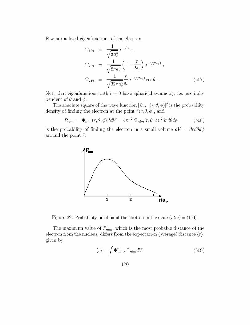
Few normalized eigenfunctions of the electron

Ψ100 =1

√

πa3o

e−r/ao ,

Ψ200 =1

√

8πa3o

(

1 − r

2ao

)

e−r/(2ao) ,

Ψ210 =1

√

32πa3o

r

aoe−r/(2ao) cos θ . (607)

Note that eigenfunctions with l = 0 have spherical symmetry, i.e. are inde-pendent of θ and φ.

The absolute square of the wave function |Ψnlm(r, θ, φ)|2 is the probabilitydensity of finding the electron at the point ~r(r, θ, φ), and

Pnlm = |Ψnlm(r, θ, φ)|2dV = 4πr2|Ψnlm(r, θ, φ)|2drdθdφ (608)

is the probability of finding the electron in a small volume dV = drdθdφaround the point ~r.

P100

1 2 r/ao

Figure 32: Probability function of the electron in the state (nlm) = (100).

The maximum value of Pnlm, which is the most probable distance of theelectron from the nucleus, differs from the expectation (average) distance 〈r〉,given by

〈r〉 =∫

Ψ∗nlmrΨnlmdV . (609)

170

Examples of the probability function Pnlm are shown in Figs. 32 and 33.

P

r/a

200

o3+ 5

Figure 33: Probability function of the electron in the state (nlm) = (200).

Interesting properties of the probability function Pnlm:

1. For n = 1, the probability has one maximum at r = ao.

2. For (n = 2, l = 0, m = 0), the probability shows two maxima locatedat r 6= n2ao.

3. Only for states such that n = l+1, the probability shows one maximumlocated at r = n2ao.

Exercise:

The normalized wave function for the ground state of a hydrogen atom hasthe form

Ψ (r) = Ae−r/ao ,

where A = 1/πa3o is a constant, ao = 4πεoh

2/me2 is the Bohr radius, and ris the distance between the electron and the nucleus. Show the following:

171

(a) The expectation value of r is 32ao.

(b) The most probable value of r is r = ao.

Solution:

(a) From the definition of expectation value, we find

〈r〉 =∫

Ψ∗ (r) rΨ (r) dV = 4πA2∫ ∞

0r3e−2βrdr ,

where β = 1/ao, and we have transformed the integral over dV into sphericalcoordinates with dV = 4πr2dr.

Performing the integration, we obtain

〈r〉 = 4πA2 6

(2β)4=

24

16

πA2

β4=

3

2π

1

πa3o

a4o =

3

2ao .

Thus, the average distance of the electron from the nucleus in the state Ψis 3/2 of the Bohr radius.

(b) The most probable value of r is that where the probability of findingthe electron is maximal.

Thus, we first calculate the probability of finding the electron at a point r:

P (r) = 4πr2|Ψ (r) |2 = 4πr2A2e−2βr =4r2

a3o

e−2βr .

Maximum of P (r) is where dP (r)/dr = 0. Hence

dP (r)

dr=

8r

a3o

e−2βr − 8βr2

a3o

e−2βr .

Thus

dP (r)

dr= 0 when βr = 1 ,

from which, we find

r =1

β= ao .

172

Note that this result agrees with the prediction of the Bohr model, that theradius of the n = 1 orbit is equal to ao.

In summary of the solution: The expectation and most probable values of rare not the same. This is because the probability curve P100(r) is not sym-metric about the maximum at ao, see Fig. 32. Thus, values of r greaterthan ao are weighted more heavily in the equation for the expectation valuethan values smaller than ao. This results in the expectation value 〈r〉 exceed-ing ao for this probability distribution.

Challenging problem: Eigenfunctions of the angular momentum

The eigenfunctions of the angular momentum L of the electron in a Hy-drogen atom for l = 1 are

Y10 (θ, φ) =

√

3

4πcos θ , Y1±1 (θ, φ) = ∓

√

3

8πsin θe±iφ .

(a) Show that the eigenfunctions are also eigenfunctions of the Lz componentof the angular momentum.

(b) Show that the eigenfunctions are not eigenfunctions of the Lx componentof the angular momentum.

(c) Find the matrix representation of Lx in the basis of the eigenfunctionsof L.

(d) Find the eigenvalues and eigenfunctions of Lx in the basis of the eigen-functions of L.

173

16 Systems of Identical Particles

Consider a system composed of N parts (subsystems), e.g. a system of Nidentical and independent particles, whose the Hamiltonian is given by

H =N∑

i=1

Hi , (610)

and the wave function is

Ψ(r) = φ1(r1)φ2(r2) . . . φN(rN) , (611)

where φi(ri) is the wave function of the ith particle located at the point rj,or equivalently we can say that φi(rj) is the wave function of the jth particlebeing in the ith state.

However, the wave function Ψ(r) is not the only eigenfunction of thesystem. For example, a wave function

Ψ(r) = φ1(r2)φ2(r1) . . . φN(rN) , (612)

is also an eigenfunction of the system with the same eigenvalue.

Proof:

Consider the eigenvalue equation with the eigenfunction (611):

HΨ(r) =N∑

i=1

HiΨ(r)

=N∑

i

Hiφ1(r1)φ2(r2) . . . φN(rN) =N∑

i=1

EiΨ(r) .

Consider now the eigenvalue equation with the eigenfunction (612)

HΨ(r) =N∑

i=1

HiΨ(r) =N∑

i

Hiφ1(r2)φ2(r1) . . . φN(rN) .

174

Since

H1φ1(r2) = E1φ1(r2) , and H2φ2(r1) = E2φ2(r1) ,

we get that HΨ(r) =∑N

i=1EiΨ(r).Even if

H1φ1(r2) = E2φ1(r2) , and H2φ2(r1) = E1φ2(r1) ,

we get that

HΨ(r) =N∑

i=1

EiΨ(r) , (613)

as required♦.

In fact there are a totalN ! permutations of φi(rj) which are eigenfunctionsof the system.

Moreover, an arbitrary linear combination of the wave functions φi(rj) isalso an eigenfunction of the system.We will illustrate this for N = 2.

16.1 Symmetrical and antisymmetrical functions

Consider an arbitrary linear combination of two wave functions

Ψ(r) =1

√

|a|2 + |b|2[aΨ(r12) + bΨ(r21)] , (614)

where Ψ(r12 = φ1(r1)φ2(r2) and Ψ(r21 = φ1(r2)φ2(r1).Then

HΨ(r) =(

H1 + H2

)

Ψ(r)

=1

√

|a|2 + |b|2[a (E1 + E2) Ψ(r12) + b (E1 + E2)Ψ(r21)]

= (E1 + E2) Ψ(r) . (615)

We know that in the linear combination |a|2/(|a|2 + |b|2) is the probabilitythat the particle ”1” is at the position r1 and the particle ”2” is at r2.

175

Equivalently, for r1 = r2, we can say that this is the probability that theparticle ”1” is in a state |1〉, and the particle ”2” is in a state |2〉.

Similarly, |b|2/(|a|2 + |b|2) is the probability that the particle ”1” is at theposition r2, and the particle ”2” is at r1.

Note, that in general, the probabilities are different. However, for twoidentical particles, the probabilities should be the same as we cannot distin-guish between two identical particles.

Thus, for two identical particles |a| = |b|. Hence, the parameters a and bcan only differ by a phase factor: b = a exp(iφ), where φ is a real number:

Ψ(r) =1√2

[

Ψ(r12) + eiφΨ(r21)]

. (616)

If we exchange the positions of the particles (r1 ↔ r2) or energy states(|1〉 ↔ |2〉), then we obtain

Ψ′(r) =1√2

[

eiφΨ(r12) + Ψ(r21)]

. (617)

Thus, the exchange of r1 ↔ r2 or |1〉 ↔ |2〉 is equivalent to multiplying Ψ(r)by eiφ and taking e2iφ = 1. Hence

eiφ = ±1 , (618)

and therefore the wave functions of identical particles are either symmetricalor antisymmetrical

Ψs(r) =1√2

[Ψ(r12) + Ψ(r21)] ,

Ψa(r) =1√2

[Ψ(r12) − Ψ(r21)] . (619)

Note that

Ψs(r12) = Ψs(r21) ,

Ψa(r12) = −Ψa(r21) . (620)

176

Properties of symmetrical and antisymmetrical functions:

1. If H = H12 = H21, i.e. the Hamiltonian is symmetrical, then HΨ(r)has the same symmetry as Ψ(r).

Proof:

Take Ψ(r) = Ψs(r). Denote f12 = H12Ψs(r12), then

f21 = H21Ψs(r21) = H12Ψs(r12) = f12 .

Take now Ψ(r) = Ψa(r). Then

f21 = H21Ψa(r21) = H12 (−Ψs(r12)) = −f12 ,

as required♦.

2. Symmetry of the wave function does not change in time, i.e. wave functioninitially symmetrical (antisymmetrical) remains symmetrical (antisymmetri-cal) for all times.

Proof:

Consider an evolution of a wave function Ψ(t) in a time dt:

Ψ(t+ dt) = Ψ(t) +∂Ψ

∂tdt .

Thus, symmetry of the wave function depends on the symmetry of ∂Ψ/∂t.From the time-dependent Schrodinger equation

ih∂Ψ

∂t= HΨ ,

we see that ∂Ψ/∂t has the same symmetry as HΨ. From the property 1, weknow that HΨ has the same symmetry as Ψ. Therefore, Ψ(t + dt) has thesame symmetry as Ψ(t),as required♦.

177

Difference between symmetric and antisymmetric functions

Antisymmetric function can be written in a form of a determinant, calledthe Slater determinant:

Ψa(r) =1√N !

∣

∣

∣

∣

∣

∣

∣

∣

∣

∣

∣

∣

∣

∣

φ1(r1) φ1(r2) . . . φ1(rN )φ2(r1) φ2(r2) . . . φ2(rN )...

φN(r1) φN(r2) . . . φN(rN)

∣

∣

∣

∣

∣

∣

∣

∣

∣

∣

∣

∣

∣

∣

, (621)

where 1/√N ! is the normalization constant.

If two particles are at the same point, r1 = r2, and then two columnsof the determinant (621) are equal, giving Ψa(r) = 0. Thus, two particlesdetermined by the antisymmetric function cannot be at the same point. Sim-ilarly, if two particles are in the same state, φ1(r1) = φ1(r2), and again twocolumns are equal giving Ψa(r) = 0.

Symmetrical function cannot be written in a form of a determinant. Thus,particles which are determined by symmetrical functions can be in the samepoint or in the same state.

Hence, particles can be divided into two types: those determined by anti-symmetric functions – called fermions, and those determined by symmetricalfunctions – called bosons.

Examples:

Fermions: electrons, protons, neutrons.Bosons: photons, π mesons, α particles.

From experiments, we know that fermions have half integer spins, whereasbosons have integer spins.

Since, an arbitrary number of bosons can be in the same state, theycan be condensated to a single state. We call this process Bose-Einsteincondensation.

178

16.2 Pauli principle

In atoms, a limited number of electrons (fermions) can occupy the same en-ergy level. How many electrons does it take to fill an energy level? Theanswer to this question is given by the Pauli principle.

Pauli principle:

No two electrons can have the same quantum numbers (n, l,m, s) ina multi-electron atom.

It is also known as the exclusion principle, for the simple reason that if anelectron has the quantum numbers (nlms) than at least one of the quantumnumbers of any further electrons must be different.

In an atom, for a given n, there are 2(2l+1) degenerate states correspondingto l = 0, 1, 2, . . ., m = −l, . . . , l, and s = − 1

2,+1

2. Thus, for a given n the

total number of electrons in the energy state Φn is

l=m∑

l=−m

2(2l + 1) = 2n2 . (622)

Following the Pauli principle, we can find numbers of electrons in theenergy states

1s , 2s , 2p , 3s , 3p , 4s , 3d , 4p , 5s , 4d , 5p

2 2 6 2 6 2 10 6 2 10 6

The Pauli principle prevents the energy states being occupied by an arbitrarynumber of electrons. The state 1s can be occupied by two electrons. Hence,as more electrons are added, the energy of the atom grows along with itssize. Thus, the Pauli principle prevents all atoms having the same size andthe same energy. This is the quantum physics explanation of atomic sizesand energies.

Since the number of electrons on given energy levels is limited, we getdifferent ground state configurations for different atoms. The ground stateof a many electron atom is that in which the electrons occupy the lowestenergy levels that they can occupy.

179

If the number of electrons for a given nl is 2(2l+ 1), we say that there isa closed shell. Examples: Helium, Beryllium, Neon.

Since the chemical properties of atoms depend on the number of electronsoutside the closed shells, the atoms with similar outer configurations will havesimilar chemical properties. Examples: The Alkali metals: Lithium (1s)22s,Sodium (1s)2(2s)2(2p)63s, and Potassium (1s)2(2s)2(2p)6(3s)2(3p)64s.This is the explanation from quantum physics of the periodic structure ofthe elements.

180

Final Remark

It is appropriate to close our lectures on quantum physics by emphasizingthe importance of quantum phenomena in the development of new areas inscience and technology. The predictions of quantum physics have turnedresearch and technology into new directions and have led to numerous tech-nological innovations and the development of a new technology on the scaleof single atoms and electrons, called quantum technology or nanotechnology.The ability to manufacture and control of the dimensions of tiny structures,such as quantum dots, allows us to engineer the unique properties of thesestructures and predict new devices such as quantum computers. The technol-ogy for creating a quantum computer is still in its infancy, but is developingvery rapidly with little sign of the progress slowing.

We have seen in our journey through the backgrounds of quantum physicsthat despite its long history, quantum physics still challenges our understand-ing, and continues to excite our imagination. Feynman in his lectures onquantum physics referred in the following way to our understanding of quan-tum physics:

”I think I can safely say that nobodyunderstands quantum mechanics.”

In summary of the subject, I think I can safely say:

”If you think you now know quantum physics,it means you do not know anything.”

Continue study of Quantum Physics with PHYS3040.

181

Appendix A

Derivation of the Boltzmann distribution function Pn

Assume that we have n identical particles (e.g. photons), each of energyE, which can occupy g identical states. The number of possible distributionsof n particles between g states is given by

t =(n+ g − 1)!

n!(g − 1)!. (623)

For example: n = 3, g = 2 gives t = 4, see Fig. 34.

We will find maximum of t with the condition that nE =const., where Eis the energy of each particle.

. .. .........Figure 34: Example of possible distributions of three particles between twostates.

Taking ln of both sides of Eq. (623), we get

ln t = ln(n+ g − 1)! − lnn! − ln(g − 1)! . (624)

Using the Sterling’s formula

lnn! = n lnn− n , (625)

and assuming that g � 1, i.e. g − 1 ≈ g, we obtain

ln t = g lnn+ g

g+ n ln

n+ g

n. (626)

183

We find maximum of ln t using the method of Lagrange undetermined multi-pliers. In this method, we construct a function

K = ln t− λnE , (627)

where λ is called a Lagrange undetermined multiplier, and find the extremum

∂K

∂n= 0 . (628)

Thus, we get

lnn

n+ g+ λE = 0 , (629)

from which, we find

n =g

eλE − 1. (630)

This is the Bose-Einstein distribution function. Since n is dimensionless, λshould be inverse of energy. We choose λ = 1/(kBT ), where kBT is theenergy of free, non-interacting particles.

When g/n� 1, we can approximate Eq. (630) by

n = ge− E

kBT , (631)

which is known in statistical physics as the Boltzmann distribution. Thisgives the number of particles n of energy E.

If there are particles, among N particles, which can have different energiesEi, then

ni

N=

g

Ne− E

kBT (632)

is the probability that ni particles of the total N particles have energy Ei.Thus, we can write

Pn = ae− E

kBT , (633)

where a is a constant.Since the probability is normalized to one (

∑

n Pn = 1), we finally get

Pn =e− E

kBT

∑

n e− E

kBT

. (634)

The sum∑

n e− E

kBT is called the partition function.

184

Appendix B: Useful mathematical formulae

Useful properties of trigonometrical functions:

sin(α± β) = sinα cos β ± sin β cosα

cos(α± β) = cosα cos β ∓ sinα sin β

sin2 α =1

2(1 − cos 2α)

cos2 α =1

2(1 + cos 2α)

∫ π

0sin3 θ dθ =

4

3

∫ 2π

0sin(mφ) sin(nφ) dφ =

{


∫ 2π

0cos(mφ) cos(nφ) dφ =

{


∫ 2π

0sin(mφ) cos(nφ) dφ = 0 for all m and n

Useful integral expressions

∫ ∞

0

x3

ex − 1dx =

π4

15

∫ ∞

−∞e−αx2

dx =

√

π

α∫ ∞

−∞xe−αx2

dx = 0

∫ ∞

−∞x2e−αx2

dx =1

2α

√

π

α

185

∫ ∞

0rne−αrdr =

n!

αn+1,

from which, we find

∫ ∞

0e−αrdr =

1

α,

∫ ∞

0re−αrdr =

1

α2,

∫ ∞

0r2e−αrdr =

2

α3,

∫ ∞

0r3e−αrdr =

6

α4

Taylor series

ωk = ωk0+β = ω0 +

(

dω

dβ

)

k0

β +1

2

(

d2ω

dβ2

)

k0

β2 + . . .

e±x = 1 ± x +x2

2!± x3

3!+ . . .

sin x = x− x3

3!+x5

5!− x7

7!+ . . .

cos x = 1 − x2

2!+x4

4!− x6

6!+ . . .

Kronecker δ function

δmn =

{

1 if m = n0 if m 6= n .

The Dirac delta function

δ(x) =

{

0 if x 6= 0∞ if x = 0 ,

such that∫ ∞

−∞f(x)δ(x)dx = f(0) ,

for any function f(x).

186

Appendix C: Physical Constants and

Conversion Factors

Bohr magneton mB = 9.724 × 10−24 [J/T]

Bohr radius ao = 5.292 × 10−11 [m]

Boltzmann constant kB = 1.381 × 10−23 [J/K]

charge of an electron e = −1.602 × 10−19 [C]

permeability of vacuum µ0 = 4π × 10−7 [H/m]

permittivity of vacuum ε0 = 8.854 × 10−12 [F/m]

Planck constant h = 6.626 × 10−34 [J.s] = 4.14 × 10−15 [eV.s]

(Planck constant)/2π h = 1.055 × 10−34 [J.s] = 6.582 × 10−16 [eV.s]

rest mass of electron me = 9.110 × 10−31 [kg]

rest mass of proton mp = 1.673 × 10−27 [kg]

Rydberg constant R = 1.097 × 107 [m−1]

speed of light in vacuum c = 2.9979 × 108 [m/s]

Stefan − Boltzmann constant σ = 5.670 × 10−8 [W/m2 · K4]

1 A = 10−10 [m] ; 1 fm = 10−15 [m] ; 1 eV = 1.602 × 10−19 [J]

1 J = 6.241 × 1018 [eV] ; π = 3.142 ; e = 2.718 .

187

quantum physics lecture notes (queensland university 2004)

Documents

good introductory

de broglie

pauli principle

potentials

heisenberg

boltzmann

algebraic

classically