quantum random access codes with shared randomness
TRANSCRIPT

Quantum Random Access Codeswith Shared Randomness
Andris Ambainisa, Debbie Leungb,
Laura Mancinskaa,b, Maris Ozolsa,b
a Department of Computing, University of Latvia,Raina bulv. 19, Riga, LV-1586, Latvia
b Department of Combinatorics and Optimization, and Institute for QuantumComputing, University of Waterloo, Waterloo, Ontario, N2L 3G1, Canada
June 12, 2009
Abstract
We consider a communication method, where the sender encodes n classical bits into 1 qubitand sends it to the receiver who performs a certain measurement depending on which of the initialbits must be recovered. This procedure is called n
p7→ 1 quantum random access code (QRAC)
where p > 1/2 is its success probability. It is known that 20.857−→ 1 and 3
0.797−→ 1 QRACs (with no
classical counterparts) exist and that 4p7→ 1 QRAC with p > 1/2 is not possible.
We extend this model with shared randomness (SR) that is accessible to both parties. Then
np7→ 1 QRAC with SR and p > 1/2 exists for any n ≥ 1. We give an upper bound on its success
probability (the known 20.857−→ 1 and 3
0.797−→ 1 QRACs match this upper bound). We discuss someparticular constructions for several small values of n.
We also study the classical counterpart of this model where n bits are encoded into 1 bit insteadof 1 qubit and SR is used. We give an optimal construction for such codes and find their successprobability exactly—it is less than in the quantum case.
Supplementary materials are available on-line athttp://home.lanet.lv/∼sd20008/racs
AA was supported by University of Latvia Grant ZP01-100 (at University of Latvia) and CIAR, NSERC, ARO,MITACS and IQC University Professorship (at University of Waterloo). DWL was funded by the CRC, ORF-RI, NSERC,CIFAR, MITACS, and Quantum-Works.
1
arX
iv:0
810.
2937
v3 [
quan
t-ph
] 1
4 Ju
n 20
09

Contents
1 Introduction 31.1 Random access codes . . . . . . . . . . . . . . . . . . . . . . . . . . . . . . . . . . . . . . 31.2 History and applications . . . . . . . . . . . . . . . . . . . . . . . . . . . . . . . . . . . . 31.3 Outline of results . . . . . . . . . . . . . . . . . . . . . . . . . . . . . . . . . . . . . . . . 4
2 Classical random access codes 42.1 Types of classical encoding-decoding strategies . . . . . . . . . . . . . . . . . . . . . . . 42.2 Yao’s principle . . . . . . . . . . . . . . . . . . . . . . . . . . . . . . . . . . . . . . . . . 52.3 Classical n 7→ 1 RAC . . . . . . . . . . . . . . . . . . . . . . . . . . . . . . . . . . . . . . 7
2.3.1 Optimal strategy . . . . . . . . . . . . . . . . . . . . . . . . . . . . . . . . . . . . 72.3.2 Asymptotic bounds . . . . . . . . . . . . . . . . . . . . . . . . . . . . . . . . . . . 8
3 Quantum random access codes 103.1 Visualizing a qubit . . . . . . . . . . . . . . . . . . . . . . . . . . . . . . . . . . . . . . . 10
3.1.1 Bloch sphere representation . . . . . . . . . . . . . . . . . . . . . . . . . . . . . . 103.1.2 Unit disk representation . . . . . . . . . . . . . . . . . . . . . . . . . . . . . . . . 12
3.2 Types of quantum encoding-decoding strategies . . . . . . . . . . . . . . . . . . . . . . . 133.3 Known quantum RACs . . . . . . . . . . . . . . . . . . . . . . . . . . . . . . . . . . . . 14
3.3.1 The 2 7→ 1 QRAC . . . . . . . . . . . . . . . . . . . . . . . . . . . . . . . . . . . 143.3.2 The 3 7→ 1 QRAC . . . . . . . . . . . . . . . . . . . . . . . . . . . . . . . . . . . 153.3.3 Impossibility of the 4 7→ 1 QRAC . . . . . . . . . . . . . . . . . . . . . . . . . . . 15
3.4 Optimal encoding for given decoding strategy . . . . . . . . . . . . . . . . . . . . . . . . 163.5 Relation to a random walk in R3 . . . . . . . . . . . . . . . . . . . . . . . . . . . . . . . 183.6 Upper bound . . . . . . . . . . . . . . . . . . . . . . . . . . . . . . . . . . . . . . . . . . 183.7 General upper bound . . . . . . . . . . . . . . . . . . . . . . . . . . . . . . . . . . . . . . 193.8 Lower bounds . . . . . . . . . . . . . . . . . . . . . . . . . . . . . . . . . . . . . . . . . . 21
3.8.1 Lower bound by random measurements . . . . . . . . . . . . . . . . . . . . . . . 213.8.2 Lower bound by orthogonal measurements . . . . . . . . . . . . . . . . . . . . . . 23
4 Constructions of QRACs with SR 234.1 Numerical results . . . . . . . . . . . . . . . . . . . . . . . . . . . . . . . . . . . . . . . . 24
4.1.1 The 2 7→ 1 and 3 7→ 1 QRACs with SR . . . . . . . . . . . . . . . . . . . . . . . . 254.1.2 The 4 7→ 1 QRAC with SR . . . . . . . . . . . . . . . . . . . . . . . . . . . . . . 254.1.3 The 5 7→ 1 QRAC with SR . . . . . . . . . . . . . . . . . . . . . . . . . . . . . . 284.1.4 The 6 7→ 1 QRAC with SR . . . . . . . . . . . . . . . . . . . . . . . . . . . . . . 304.1.5 The 9 7→ 1 QRAC with SR . . . . . . . . . . . . . . . . . . . . . . . . . . . . . . 33
4.2 Symmetric constructions . . . . . . . . . . . . . . . . . . . . . . . . . . . . . . . . . . . . 354.2.1 Symmetric great circle arrangements . . . . . . . . . . . . . . . . . . . . . . . . . 354.2.2 Symmetric 4 7→ 1 QRAC with SR . . . . . . . . . . . . . . . . . . . . . . . . . . 384.2.3 Symmetric 6 7→ 1 QRAC with SR . . . . . . . . . . . . . . . . . . . . . . . . . . 414.2.4 Symmetric 9 7→ 1 QRAC with SR . . . . . . . . . . . . . . . . . . . . . . . . . . 414.2.5 Symmetric 15 7→ 1 QRAC with SR . . . . . . . . . . . . . . . . . . . . . . . . . . 42
4.3 Discussion . . . . . . . . . . . . . . . . . . . . . . . . . . . . . . . . . . . . . . . . . . . . 42
5 Conclusion 445.1 Summary . . . . . . . . . . . . . . . . . . . . . . . . . . . . . . . . . . . . . . . . . . . . 445.2 Open problems for n 7→ 1 QRACs . . . . . . . . . . . . . . . . . . . . . . . . . . . . . . . 445.3 Possible generalizations . . . . . . . . . . . . . . . . . . . . . . . . . . . . . . . . . . . . 455.4 Acknowledgments . . . . . . . . . . . . . . . . . . . . . . . . . . . . . . . . . . . . . . . . 47
A Combinatorial interpretation of sums 47
B POVMs versus orthogonal measurements 48
2

1 Introduction
1.1 Random access codes
In general random access code (or simply RAC) stands for “encoding a long message into fewer bitswith the ability to recover (decode) any one of the initial bits (with some probability of success)”. Arandom access code can be characterized by the symbol “n
p7→ m” meaning that n bits are encoded intom and any one of the initial bits can be recovered with probability at least p. We require that p > 1/2since p = 1/2 can be achieved by guessing. In this paper we consider only the case when m = 1. So wehave the following problem:
Problem (Classical). There are two parties—Alice and Bob. Alice is asked to encode some classicaln-bit string into 1 bit and send this bit to Bob. We want Bob to be able to recover any one of the ninitial bits with high success probability.
Note that Alice does not know in advance which bit Bob will need to recover, so she cannot sendonly that bit. If they share a quantum channel then we have the quantum version of the previousproblem:
Problem (Quantum). Alice must encode her classical n-bit message into 1 qubit (quantum bit) andsend it to Bob. He performs some measurement on the received qubit to extract the required bit (themeasurement that is used depends on which bit is needed).
Both problems look similar, however the quantum version has an important feature. In the classicalcase the fact that Bob can recover any one of the initial bits implies that he can actually recover all ofthem—each with high probability of success. Surprisingly in the quantum case this is not true, becauseafter the first measurement the state of the qubit will be disturbed and further attempts to extractmore information can fail.
1.2 History and applications
As noted in [6, 8], the idea behind quantum random access codes or QRACs is very old (relative toquantum information standards). It first appeared in a paper by Stephen Wiesner [1] published in 1983and was called conjugate coding. Later these codes were re-discovered by Ambainis et al. in [2, 3]. Theyshow that there exists 2 0.857−→ 1 QRAC and mention its immediate generalization to 3 0.797−→ 1 QRAC dueto Chuang (see also [5] and [8] for more details). However, Hayashi et al. [5] show that it is impossibleto construct a 4
p7→ 1 QRAC with p > 1/2. We will discuss these results more in Sect. 3.3.There has also been work on n
p7→ m codes with m > 1, see [2, 3, 4]. Ambainis et al. [2] show that ifa n
p7→ m QRAC with p > 1/2 exists, then m = Ω(n/ log n), which was later improved by Nayak [4, 3]to m ≥ (1−H(p))n, where H(p) = −p log p− (1− p) log(1− p) is the binary entropy function. Othergeneralizations include: considering d-valued bits instead of qubits [6, 8] and recovering several ratherthan a single bit [16].
Originally quantum random access codes were studied in the context of quantum finite automata[2, 3, 4]. However, they also have applications in quantum communication complexity [6, 9, 10, 11], inparticular for network coding [5, 12] and locally decodable codes [13, 14, 15, 16]. Recently results onquantum random access codes have been applied for quantum state learning [17].
Experimental feasibility of QRACs and their relation to contextuality and non-locality has beendiscussed in [6, Chapter 7]. Recently a similar protocol called parity-oblivious multiplexing has beenconsidered in [7]. It has an additional cryptographic constraint that Alice is not allowed to transmitany information about the parity of the input string. In addition [7] also discuss the first experimentaldemonstration of 2 7→ 1 and 3 7→ 1 QRACs.
We want to emphasize the setting in which the impossibility of 4p7→ 1 QRAC with p > 1/2 was proved
in [5]: Alice is allowed to perform a locally randomized encoding of the given string into a one-qubitstate and Bob is allowed to perform different positive operator-valued measure (POVM) measurementsto recover different bits. This is the most general setting when information is encoded into a one-qubit
3

state and both parties are allowed to use randomized strategies, but only have access to local coins.However, we can consider an even more general setting—when both parties share a common coin. Thismeans that Alice and Bob are allowed to cooperate by using some shared source of randomness to agreeon which strategy to use. We will refer to this source as a shared random string or shared randomness(SR). Note that shared randomness is a more powerful resource than local randomness, since parts ofthe shared random string can be exclusively used only by Alice or Bob to simulate local coins. It turnsout that in this new setting 4
p7→ 1 QRAC is possible with p > 1/2. In fact, np7→ 1 QRACs with p > 1/2
can be constructed for all n ≥ 1 (see Sect. 3.8).
1.3 Outline of results
In Sect. 2 we study classical n 7→ 1 random access codes with shared randomness. In Sect. 2.2 weintroduce Yao’s principle that is useful for understanding both classical and quantum codes. A classicalcode that is optimal for all n is presented in Sect. 2.3.1 and the asymptotic behavior of its successprobability is considered in Sect. 2.3.2.
In Sect. 3 we study quantum random access codes with shared randomness. In Sect. 3.3 we discusswhat is known in the case when shared randomness is not allowed, i.e., 2 7→ 1 and 3 7→ 1 QRACs andthe impossibility of 4 7→ 1 QRAC. In Sect. 3.6 we give an upper bound of success probability of QRACswith SR and generalize it in Sect. 3.7 for POVM measurements. In Sect. 3.8 we give two constructionsof n
p7→ 1 QRAC with SR and p > 1/2 for all n ≥ 2 that provide a lower bound for success probability.In Sect. 4 we try to find optimal QRACs with SR for several small values of n. In particular, in
Sect. 4.1 we discuss QRACs obtained by numerical optimization, and in Sect. 4.2 we consider symmetricconstructions.
Finally, we conclude in Sect. 5 with a summary of the obtained results (Sect. 5.1), a list of openproblems (Sect. 5.2) and possible generalizations (Sect. 5.3).
2 Classical random access codes
2.1 Types of classical encoding-decoding strategies
As a synonym for random access code we will use the term strategy to refer to the joint encoding-decoding scheme used by Alice and Bob. Two measures of how good the strategy is will be used: theworst case success probability and the average success probability. Both probabilities must be calculatedover all possible pairs (x, i) where x ∈ 0, 1n is the input and i ∈ 1, . . . , n indicates which bit mustbe recovered. We are interested in the worst case success probability, but in our case according to Yao’sprinciple (introduced in Sect. 2.2) the average success probability can be used to estimate it.
Depending on the computational model considered, different types of strategies are allowed. Thesimplest type corresponds to Alice and Bob acting deterministically and independently.
Definition. A pure classical n 7→ 1 encoding-decoding strategy is an ordered tuple (E,D1, . . . , Dn) thatconsists of an encoding function E : 0, 1n 7→ 0, 1 and n decoding functions Di : 0, 1 7→ 0, 1.
These limited strategies yield RACs with poor performance. This is because Bob can recover all bitscorrectly for no more than two input strings, since he receives either 0 or 1 and acts deterministicallyin each case. For all other strings at least one bit will definitely be recovered incorrectly, thereforethe worst case success probability is 0. If we allow Alice and Bob to act probabilistically but withoutcooperation, then we get mixed strategies.
Definition. A mixed classical n 7→ 1 encoding-decoding strategy is an ordered tuple (PE , PD1 , . . . , PDn)
of probability distributions. PE is a distribution over encoding functions and PDiover decoding func-
tions.
It is obvious that in this setting the worst case probability is at least 1/2. This is obtained byguessing—we output either 0 or 1 with probability 1/2 regardless of the input. Formally this meansthat for each i, PDi
is a uniform distribution over two constant decoding functions 0 and 1. It has been
4

shown that in this setting for 2 7→ 1 case one cannot do better than guessing, i.e., there is no 2p7→ 1
RAC with worst case success probability p > 1/2 [2, 3].However, we can allow cooperation between Alice and Bob—they can use a shared random string
to agree on some joint strategy.
Definition. A classical n 7→ 1 encoding-decoding strategy with shared randomness is a probabilitydistribution over pure classical strategies.
Note that this is the most general randomized setting, since both randomized cooperation and localrandomization are possible. This is demonstrated in the following example.
Example. Consider the following strategy: randomly agree on i ∈ 1, . . . , n and send the ith bit; ifthe ith bit is requested, output the received bit, otherwise guess. This strategy can formally be specifiedas follows: uniformly choose a pure strategy from the set⋃
i∈1,...,n
(ei, c1, . . . , ci−1, d, g1, . . . , gn−i) | c ∈ d0, d1i−1
, g ∈ d0, d1n−i, (1)
where the encoding function ei is given by ei(x) = xi and decoding functions d0, d1, and d are given byd0(b) = 0, d1(b) = 1, and d(b) = b, where b is the received bit. The total amount of required randomnessis n−1+log n bits, because one out of n ·2n−1 pure strategies must be selected. Note that only log n ofthese bits must be shared among Alice and Bob, so that they can agree on the value of i. The remainingn− 1 random bits are needed only by Bob for choosing random decoding functions c ∈ d0, d1i−1 andg ∈ d0, d1n−i.
Note that the amount of randomness used in the above example can be reduced. Since only one bitmust be recovered, there is no need to choose each of the decoding functions independently. Thus Bobneeds only one random bit that he will output whenever some bit other than the ith bit is requested.This is illustrated in the next example.
Example. Alice and Bob uniformly sample a pure strategy from the following set:(ei, c, . . . , c︸ ︷︷ ︸
i−1
, d, c, . . . , c︸ ︷︷ ︸n−i
) | 1 ≤ i ≤ n, c ∈ d0, d1. (2)
This requires log n random bits to be shared among Alice and Bob and 1 private random bit for Bob,i.e., 1 + log n random bits in total.
We are interested in classical strategies with SR, because they provide a classical analogue of QRACswith SR. However, in this setting finding the optimal strategy seems to be hard, therefore we will turnto Yao’s principle for help.
2.2 Yao’s principle
When dealing with randomized algorithms, it is hard to draw general conclusions (like proving optimalityof a certain randomized algorithm) because the possible algorithms may form a continuum. In suchsituations it is very helpful to apply Yao’s principle [18]. This allows us to shift the randomness in thealgorithm to the input and consider only deterministic algorithms.
Let S be a classical strategy with SR. One can think of it as a stochastic process consisting of applyingthe encoding map E to the input x, followed by applying the decoding map Di to the ith bit. Both ofthese maps depend on the value of the shared random string. The result of S is S(x, i) = Di(E(x)),which is a stochastic variable over the set 0, 1. Let Pr[S(x, i) = xi] denote the probability that thestochastic variable S(x, i) takes value xi. Then the worst case success probability of the optimal classicalstrategy with SR is given by
maxS
minx,i
Pr[S(x, i) = xi]. (3)
5

Let µ be some distribution over the input set 0, 1n×1, . . . , n and let Prµ[P(x, i) = xi] denote theexpected success probability of a pure (deterministic) strategy P. If the “hardest” input distribution ischosen as µ, then the expected success probability of the best pure strategy for this distribution is
minµ
maxP
Prµ[P(x, i) = xi]. (4)
Yao’s principle states that the quantities given in (3) and (4) are equal [18]:
maxS
minx,i
Pr[S(x, i) = xi] = minµ
maxP
Prµ[P(x, i) = xi]. (5)
Thus Yao’s principle provides us with an upper bound for the worst case probability (3). All we haveto do is to choose an arbitrary input distribution µ0 and find the best pure strategy P0 for it. Thenaccording to Yao’s principle we have
Prµ0 [P0(x, i) = xi] ≥ maxS
minx,i
Pr[S(x, i) = xi], (6)
with equality if and only if µ0 is the “hardest” distribution. It turns out that for random access codesthe uniform distribution η is the “hardest”. To prove it, we must first consider the randomizationlemma.
Lemma 1. ∀P∃S : minx,i Pr[S(x, i) = xi] = Prη[P(x, i) = xi], where η is the uniform distribution. Inother words: the worst case success probability of S is the same as the average case success probabilityof P with uniformly distributed input.
Proof. This can be achieved by randomizing the input with the help of the shared random string.Alice’s input can be randomized by XOR-ing it with an n-bit random string r. But Bob’s input canbe randomized by adding (modulo n) a random number d ∈ 0, . . . , n− 1 to it (assume for now thatbits are numbered from 0 to n− 1). To obtain a consistent strategy, these actions must be identicallyperformed on both sides, thus a shared random string of n + log n bits1 is required. Assume that Eand Di are the encoding and decoding functions of the pure strategy P; then the new strategy S is
E′(x) = E(Shiftd(x⊕ r)), (7)D′i(b) = Di+d mod n(b)⊕ ri, (8)
where Shiftd(s) substitutes si+d mod n by si in string s. Due to input randomization, this strategy hasthe same success probability for all inputs (x, i), namely
Pr[S(x, i) = xi] =∑
y∈0,1n
n−1∑j=0
12n · n
Pr[P(y, j) = yj ] = Prη[P(y, j) = yj ], (9)
coinciding with the average success probability of the pure strategy P.
Now we will show that inequality (6) becomes an equality when µ0 = η, meaning that the uniformdistribution η is the “hardest”.
Lemma 2. The minimum of (4) is reached at the uniform distribution η, i.e.,
minµ
maxP
Prµ[P(x, i) = xi] = maxP
Prη[P(x, i) = xi]. (10)
Proof. From the previous Lemma we know that there exists a strategy with SR S0 such that
minx,i
Pr[S0(x, i) = xi] = maxP
Prη[P(x, i) = xi] (11)
1We will not worry about how Bob obtains a uniformly distributed d from a string of random bits when n 6= 2k.
6

(S0 is obtained from the best pure strategy by prepending it with input randomization). However,among all strategies with SR there might be one that is better than S0, thus
maxS
minx,i
Pr[S(x, i) = xi] ≥ maxP
Prη[P(x, i) = xi]. (12)
But if we put µ0 = η into inequality (6), we obtain
maxP
Prη[P(x, i) = xi] ≥ maxS
minx,i
Pr[S(x, i) = xi], (13)
which is the same as (12), but with reversed sign. This means that both sides are actually equal:
maxP
Prη[P(x, i) = xi] = maxS
minx,i
Pr[S(x, i) = xi]. (14)
Applying Yao’s principle to the right hand side of (14) we obtain the desired equation (10).
Theorem 1. For any pure strategy P
Prη[P(x, i) = xi] ≤ maxS
minx,i
Pr[S(x, i) = xi], (15)
with equality if and only if P is optimal for the uniform distribution η.
Proof. To obtain the required inequality, do not maximize the left hand side of equation (14), but putan arbitrary P. It is obvious that we will obtain equality if and only if P is optimal.
This theorem has important consequences—it allows us to consider pure strategies with uniformlydistributed input rather than strategies with SR. If we manage to find the optimal pure strategy, thenwe can also construct an optimal strategy with SR using input randomization2. If the pure strategy isnot optimal, then we get a lower bound for the strategy with SR.
2.3 Classical n 7→ 1 RAC
Before considering n 7→ 1 QRACs with shared randomness, we will find an optimal classical n 7→ 1RAC with shared randomness and derive bounds for it.
2.3.1 Optimal strategy
According to Theorem 1 we can consider only pure strategies. As a pure strategy is deterministic, foreach input it gives either a correct or a wrong answer. To maximize the average success probability wemust find a pure strategy that gives the correct answer for as many of the n ·2n inputs as possible—sucha strategy we will call an optimal pure strategy.
Let us first consider the problem of finding an optimal decoding strategy, when the encoding strategyis fixed. An encoding function E : 0, 1n 7→ 0, 1 divides the set of all strings into two parts:
X0 = x ∈ 0, 1n | E(x) = 0 ,X1 = x ∈ 0, 1n | E(x) = 1 .
(16)
If Bob receives bit b, he knows that the initial string was definitely from the set Xb, but there is no wayfor him to tell exactly which string it was. However, if he must recover only the ith bit, he can checkwhether there are more zeros or ones among the ith bits of strings from set Xb. More formally, we canintroduce the symbol N b
i (k) that denotes the number of strings from set Xb that have the bit k in ithposition:
N bi (k) = |x ∈ Xb | xi = k| , (17)
2If the encoding function depends only on the Hamming weight of the input string x (e.g., majority function) and thedecoding function does not depend on i, there is no need to randomize over i, so n instead of n + log n shared randombits are enough.
7

Therefore the optimal decoding strategy Di : 0, 1 7→ 0, 1 for the ith bit is
Di(b) =
0 if N b
i (0) ≥ N bi (1),
1 otherwise.(18)
Of course, if N bi (0) = N b
i (1), Bob can output 1 as well. For pure strategies there are only 4 possibledecoding functions for each bit: 0, 1, b, or NOT b. But this is still quite a lot so we will consider thetwo following lemmas. The first lemma will rule out the constant decoding functions 0 and 1.
Lemma 3. For any n there exists an optimal pure classical n 7→ 1 RAC that does not use constantdecoding functions 0 and 1 for any bits.
Proof. We will show that if there exists an optimal strategy that contains constant decoding functionsfor some bits, then there also exists an optimal strategy that does not. Let us assume that there is anoptimal strategy with constant decoding function 0 for the ith bit (the same argument goes throughfor 1 as well). Then according to equation (18) we have N0
i (0) ≥ N0i (1) and N1
i (0) ≥ N1i (1). Note that
N0i (0) + N1
i (0) = N0i (1) + N1
i (1) = 2n−1, because xi = 0 in exactly half of all 2n strings. This meansthat actually N0
i (0) = N0i (1) and N1
i (0) = N1i (1). If we take a look at (18) again, we see that in such
situation any decoding strategy is optimal and we can use any non-constant strategy instead.
Lemma 4. For any n there exists an optimal pure classical n 7→ 1 RAC that does not use decodingfunction NOT b for any bits.
Proof. We will show that for each pure strategy P that uses negation as the decoding function for theith bit, there exists a pure strategy P ′ with the same average case success probability that does not.If P consists of encoding function E and decoding functions Dj , then P ′ can be obtained from P byinverting the ith bit before encoding and after decoding:
E′(x) = E(NOTi x), (19)
D′j(b) =
NOTDj(b) if j = i,Dj(b) otherwise,
(20)
where NOTi inverts the ith bit of string. It is obvious that P and P ′ have the same average successprobabilities, because if P gives the correct answer for input (x, i) then P ′ gives the correct answer forinput (NOTi x, i). The same holds for wrong answers.
Theorem 2. The pure classical n 7→ 1 RAC with identity decoding functions and majority encodingfunction is optimal.
Proof. According to Lemma 3 and Lemma 4, there exists an optimal pure classical n 7→ 1 RAC withidentity decoding function for all bits. Now we must consider the other part—finding an optimalencoding given a particular (identity) decoding function. It is obvious that in our case optimal encodingmust return the majority of bits:
E′(x) =
0 if |x| < n/2,1 otherwise,
(21)
where |x| is the Hamming weight of string x (the number of ones in it).
2.3.2 Asymptotic bounds
Let us find the exact value of the average success probability for the optimal pure RAC suggested inTheorem 2. We will separately consider the even and odd cases.
In the odd case (n = 2m+ 1) the average success probability is given by
p(2m+ 1) =1
(2m+ 1) · 22m+1
(2
2m+1∑i=m+1
i
(2m+ 1
i
)), (22)
8

2 3 4 5 6 7 8 9 10 11 12 13 14 15n
0.6
0.7
0.8
0.9
pHnL
Figure 1: Exact probability of success p(n) for optimal pure classical n 7→ 1 RAC (black dots) accordingto (24) and its approximate value (dashed line) according to (27). Dotted lines show upper and lowerbounds of p(n) for odd and even n according to inequalities (29) and (30).
where the factor 2 stands for either zeros or ones being the majority, and(2m+1i
)stands for the number
of strings where the given symbol dominates and appears exactly i times.In the even case (n = 2m) there are a lot of strings with the same number of zeros and ones. These
strings are bad, because with majority encoding and identity decoding it is not possible to give thecorrect answer for more than half of all bits. The corresponding average success probability is given by
p(2m) =1
2m · 22m
(2
2m∑i=m+1
i
(2mi
)+m
(2mm
)), (23)
where the last term stands for the bad strings.In Appendix A we give a combinatorial interpretation of the sums in (22) and (23). Equations (143)
and (144) derived in Appendix A can be used to simplify p(2m + 1) and p(2m), respectively. It turnsout that both probabilities are equal:
p(2m) = p(2m+ 1) =12
+1
22m+1
(2mm
). (24)
These two expressions can be combined as follows:
p(n) =12
+12n
(n− 1⌊n−1
2
⌋). (25)
We can apply Stirling’s approximation [20] m! ≈(me
)m√2πm to (24) and obtain
p(2m) = p(2m+ 1) ≈ 12
+1
2√πm
. (26)
If we put m ≈ n2 , then (26) turns to
p(n) ≈ 12
+1√2πn
. (27)
9

We see that the value of (27) approaches 1/2 as n increases. Thus the obtained codes are not verygood for large n, since p = 1/2 can be obtained by guessing. We will observe a similar (but slightlybetter) behavior also in the quantum case. The exact probability (24) and its approximation (27) areshown in Fig. 1.
For odd and even cases asymptotic upper and lower bounds on p(n) can be obtained using thefollowing inequality [20]: √
2πn(ne
)ne
112n+1 < n! <
√2πn
(ne
)ne
112n . (28)
For the odd case we have
exp(
112n−11 −
26n−6
)√
2π(n− 1)< p(n)− 1
2<
exp(
112n−12 −
26n−5
)√
2π(n− 1), (29)
but for the even case
exp(
112n −
26n+1
)√
2πn< p(n)− 1
2<
exp(
112n+1 −
26n
)√
2πn. (30)
All four bounds are shown in Fig. 1.
3 Quantum random access codes
3.1 Visualizing a qubit
When dealing with quantum random access codes (at least in the qubit case), it is a good idea to tryto visualize them. We provide two ways.
3.1.1 Bloch sphere representation
A pure qubit state is a column vector |ψ〉 ∈ C2. It can be expressed as a linear combination |ψ〉 =α |0〉 + β |1〉, where |0〉 =
(10
)and |1〉 =
(01
). The coefficients α, β ∈ C must satisfy |α|2 + |β|2 = 1.
Since the physical state is not affected by the phase factor (i.e., |ψ〉 and eiφ |ψ〉 are the same states forany φ ∈ R), without the loss of generality one can write
|ψ〉 =(
cos θ2eiϕ sin θ
2
), (31)
where 0 ≤ θ ≤ π and 0 ≤ ϕ < 2π (the factor 1/2 for θ in (31) is chosen so that these ranges resemblethe ones for spherical coordinates in R3).
For almost all states |ψ〉 there is a unique way to assign the parameters θ and ϕ. The only exceptionsare states |0〉 and |1〉, that correspond to θ = 0 and θ = π, respectively. In both cases ϕ does not affectthe physical state. Note that the spherical coordinates with latitude θ and longitude ϕ have the sameproperty, namely—the longitude is not defined at poles. This suggests that the state space of a singlequbit is topologically a sphere.
Indeed, there is a one-to-one correspondence between pure qubit states and the points on a unitsphere in R3. This is called the Bloch sphere representation of a qubit state. The Bloch vector for state(31) is r = (x, y, z), where the coordinates (see Fig. 2) are given by
x = sin θ cosϕ,y = sin θ sinϕ,z = cos θ.
(32)
Given the Bloch vector r = (x, y, z), the coefficients of the corresponding state |ψ〉 = α |0〉 + β |1〉 canbe found as follows [19, pp. 102]:
α =
√z + 1
2, β =
x+ iy√2(z + 1)
(33)
10

ÈΨ\
Θ
j
x
y
z
Figure 2: Angles θ and ϕ of the Blochvector corresponding to state |ψ〉.
ÈΨ\
ÈΨ0\
ÈΨ1\
Α
d0
d1
Figure 3: Geometric interpretation of or-thogonal measurement.
with the convention that (0, 0,−1) corresponds to α = 0 and β = 1.The density matrix of a pure state |ψ〉 is defined as ρ = |ψ〉〈ψ|. For the state |ψ〉 in (31) we have
ρ =12
(1 + cos θ e−iϕ sin θeiϕ sin θ 1− cos θ
)=
12
(I + xσx + yσy + zσz) , (34)
where (x, y, z) are the coordinates of the Bloch vector r given in (32) and
I =(
1 00 1
), σx =
(0 11 0
), σy =
(0 −ii 0
), σz =
(1 00 −1
)(35)
are called Pauli matrices. We can write (34) more concisely as
ρ =12
(I + r · σ) (36)
where r = (x, y, z) and σ = (σx, σy, σz).If r1 and r2 are the Bloch vectors of two pure states |ψ1〉 and |ψ2〉, then
|〈ψ1|ψ2〉|2 = Tr(ρ1ρ2) =12
(1 + r1 · r2). (37)
This relates the inner product in C2 to the one in R3. Since r1 and r2 are unit vectors, r1 · r2 = cosα,where α is the angle between r1 and r2.
An orthogonal measurement M on a qubit can be specified by a set of two orthonormal states:M = |ψ0〉 , |ψ1〉. Orthonormality means that 〈ψi|ψj〉 = δij . If we measure a qubit that is in state |ψ〉with measurement M then the outcome will be either 0 or 1 and the state will “collapse” to |ψ0〉 or |ψ1〉with probabilities |〈ψ0|ψ〉|2 and |〈ψ1|ψ〉|2, respectively. Observe that for orthogonal states equation (37)implies r1 · r2 = −1, therefore they correspond to antipodal points on the Bloch sphere. If we denotethe angle between the Bloch vectors of |ψ〉 and |ψ0〉 by α, then according to (37) the probabilities ofthe outcomes are
p0 =12
(1 + cosα),
p1 =12
(1− cosα).(38)
There is a nice geometrical interpretation of these probabilities. If we project the Bloch vector corre-sponding to |ψ〉 on the axes spanned by the Bloch vectors of |ψ0〉 and |ψ1〉 (see Fig. 3), then p0 = d1/2
11

Figure 4: Curves of constant θ and ϕ before (on the left) and after the Hadamard transformation (onthe right). Initially the curves of constant θ are concentric circles, but after the transformation theyappear as deformed circles around both poles. The curves of constant ϕ transform form radial rays to“field lines” connecting both poles. The image on the left appears to have only the North pole |0〉, sincethe Bloch sphere is punctured at the South pole |1〉 which must be identified with the boundary of theunit disk. The “left pole” and “right pole” in the image on the right correspond to the states |1〉 and|0〉, respectively.
and p1 = d0/2 (note the different indices), where d0 is the distance between the projection and |ψ0〉,but d1 is the distance between the projection and |ψ1〉. Observe that vectors on the upper hemispherehave greater probability to collapse to |ψ0〉, but on lower hemisphere, to |ψ1〉. On the equator bothprobabilities are equal to 1
2 .
3.1.2 Unit disk representation
There is another way of visualizing a qubit. Unlike the Bloch sphere representation, this way of repre-senting a qubit is not known to have appeared elsewhere. The idea is to use only one complex numberto specify a pure qubit state |ψ〉 =
( αβ
)∈ C2. This is possible since |ψ〉 can be written in the form (31),
which is completely determined by its second component
β = eiϕ sinθ
2. (39)
The first component is just√
1− |β|2 = α. As |β| ≤ 1, the set of all possible qubit states can beidentified with a unit disk in the complex plane (the polar coordinates assigned to |ψ〉 are (r, ϕ), wherer = sin θ
2 ). The origin β = 0 corresponds to |ψ〉 = |0〉, and all points on the unit circle |β| = 1 areidentified with |ψ〉 = |1〉, since eiϕ |1〉 corresponds to the same quantum state for all ϕ ∈ R.
The relation between the unit disk representation and the Bloch sphere representation can be visu-alized as follows:
• the unit disk is obtained by puncturing the Bloch sphere at its South pole and flattening it,
• the Bloch sphere is obtained by gluing together the boundary of the unit disk.
It is much harder to visualize how a unitary transformation acts in the unit disk representation. Letus consider a simple example.
12

Example. Let us consider the action of the Hadamard gate H = 1√2
(1 11 −1
)in the unit disk represen-
tation. Note that H2 = I thus H is an involution (self-inverse). It acts on the standard basis states asfollows:
H |0〉 = 1√2|0〉+ 1√
2|1〉 = |+〉 , (40)
H |1〉 = 1√2|0〉 − 1√
2|1〉 = |−〉 . (41)
The way H transforms the curves of constant θ and ϕ is shown in Fig. 4. From equation (40) we seethat the origin β = 0 corresponding to |0〉 is mapped to the “right pole” β = 1√
2corresponding to |+〉
(and vice versa). Recall that all points on the boundary of the unit disk in Fig. 4 (on the left) areidentified with |1〉. Thus equation (41) tells us that the unit circle |β| = 1 is mapped to the “left pole”β = − 1√
2in Fig. 4 (on the right) corresponding to |−〉 (and vice versa). This means that |−〉 is mapped
to the boundary of the unit disk in Fig. 4 (on the right).
Since we use only one complex number β to represent a quantum state, a finite set of quantumstates β1, β2, . . . , βn can be represented by a polynomial
c (β − β1)(β − β2) · · · (β − βn) (42)
whose roots are βi (here c 6= 0 is arbitrary). We will use this representation in Sects. 3.3 and 4.1 todescribe the qubit states whose Bloch vectors are the vertices of certain polyhedra. It is surprising thatfor those states the values of c can be chosen so that the resulting polynomials have integer coefficients.
3.2 Types of quantum encoding-decoding strategies
Let us now consider the quantum analogue of a pure strategy.
Definition. A pure quantum n 7→ 1 encoding-decoding strategy is an ordered tuple (E,M1, . . . ,Mn) thatconsists of encoding function E : 0, 1n 7→ C2 and n orthogonal measurements: Mi =
∣∣ψi0⟩ , ∣∣ψi1⟩.
If Alice encodes the string x with function E, she obtains a pure qubit state |ψ〉 = E(x). When Bobreceives |ψ〉 and is asked to recover the ith bit of x, he performs the measurement Mi. The probabilitythat Bob recovers xi correctly is equal to
p(x, i) =∣∣⟨ψixi
∣∣ψ⟩∣∣2 . (43)
As in the classical setting, we can allow Alice and Bob to have probabilistic quantum strategieswithout cooperation. Though we will not need it, mixed quantum strategies can be defined in completeanalogy with mixed classical strategies.
Definition. A mixed quantum n 7→ 1 encoding-decoding strategy is an ordered tuple (PE , PM1 , . . . , PMn)
of probability distributions. PE is a distribution over encoding functions E and PMiare probability
distributions over orthogonal measurements of qubit.
The main objects of our research are quantum strategies with cooperation, i.e., with shared ran-domness. They are defined in complete analogy with the classical ones.
Definition. A quantum n 7→ 1 encoding-decoding strategy with shared randomness is a probabilitydistribution over pure quantum strategies.
We would like to point out two very important things about quantum strategies with shared ran-domness. The first thing is that all statements about classical strategies with SR in Sect. 2.2 are validfor quantum strategies as well (the only difference is that “pure strategy” now means “pure quantumstrategy” instead of “pure classical strategy” and “strategy with SR” means “quantum strategy withSR” instead of “classical strategy with SR”). The most important consequence of this observation isthat Theorem 1 is valid also for quantum strategies with SR. This means that the same technique ofobtaining the upper bound can be used in the quantum case, i.e., we can consider the average success
13

x
y
z
0001
1011
Figure 5: Bloch sphere representation ofencoding for 2 7→ 1 quantum random ac-cess code.
x
y
z
000
001
010
011
100
101
110
111
Figure 6: Bloch sphere representation ofencoding for 3 7→ 1 quantum random ac-cess code.
probability of a pure quantum strategy instead of the worst case success probability of the quantumstrategy with SR.
The second thing is that the quantum strategy with SR is the most powerful quantum encoding-decoding strategy when both kinds of classical randomness (local and shared) is allowed. However, it isnot the most general strategy, since it cannot be used to simulate certain classical strategies, e.g., theones with fixed output. However, it turns out that the ability to simulate such strategies does not giveany advantage (see Sect. 3.7 and Appendix B).
3.3 Known quantum RACs
In [2, 3] it has been shown that for 2 7→ 1 classical RACs in the mixed setting the decoding partycannot do better than guessing, i.e., the worst case success probability cannot exceed 1/2. However,if quantum states can be transmitted, there are pure quantum 2 7→ 1 and 3 7→ 1 schemes [2, 3]. Thisclearly indicates the advantages of quantum RACs. On the other hand, a quantum 4 7→ 1 schemecannot exist [5]. We will review these results in the next three sections.
3.3.1 The 2 7→ 1 QRAC
The 2 7→ 1 QRAC is described in [2, 3, 5]. The main idea is to use two mutually orthogonal pairs ofantipodal Bloch vectors for measurement bases. For example, let M1 and M2 be the measurements alongthe x and y axes, respectively. The corresponding Bloch vectors are v1 = (±1, 0, 0) and v2 = (0,±1, 0).The measurement bases are
M1 =
1√2
(11
),
1√2
(1−1
), (44)
M2 =
1√2
(1i
),
1√2
(1−i
). (45)
The planes orthogonal to the x and y axes cut the Bloch sphere into four parts. Note that in each partonly one definite string can be encoded (otherwise the worst case success probability will be less than 1
2 ).According to (38), all encoding points must be as far from both planes as possible in order to maximizethe worst case success probability (recall the geometrical interpretation of the measurement shown inFig. 3). In our case the best encoding states are the vertices of a square 1√
2(±1,±1, 0) inscribed in the
unit circle on the xy plane (see Fig. 5). Given a string x = x1x2, the Bloch vector of the encoding state
14

can be found as follows:
r(x) =1√2
(−1)x1
(−1)x2
0
. (46)
The corresponding encoding function is
E(x1, x2) =1√2|0〉+
(−1)x1 + i(−1)x2
2|1〉 . (47)
The success probability is the same for all input strings and all bits to be recovered:
p =12
(1 + cos
π
4
)=
12
+1
2√
2≈ 0.853553. (48)
3.3.2 The 3 7→ 1 QRAC
It is not hard to generalize the 2 7→ 1 QRAC to a 3 7→ 1 code—just take three mutually orthogonal pairsof antipodal Bloch vectors, i.e., the vertices of an octahedron [5, 8]. The third pair is v3 = (0, 0,±1)and the corresponding measurement basis is
M3 =(
10
),
(01
). (49)
In this case we have three orthogonal planes that cut the sphere into eight parts and only one stringcan be encoded into each part. In this case the optimal encoding states correspond to the vertices of acube 1√
3(±1,±1,±1) inscribed in the Bloch sphere (see Fig. 6). The Bloch vector of the encoding state
of string x = x1x2x3 is
r(x) =1√3
(−1)x1
(−1)x2
(−1)x3
. (50)
The corresponding encoding function is E(x1, x2, x3) = α |0〉+ β |1〉 with coefficients α and β explicitlygiven by
α =
√12
+(−1)x3
2√
3,
β =(−1)x1 + i(−1)x2√
6 + 2√
3(−1)x3
.
(51)
In fact, the coefficients β are exactly the eight roots of the polynomial3
36β8 + 24β4 + 1 (52)
This code also has the same success probability in all cases:
p =12
+1
2√
3≈ 0.788675. (53)
3.3.3 Impossibility of the 4 7→ 1 QRAC
Hayashi et al. [5] have shown that 2 7→ 1 and 3 7→ 1 codes discussed above cannot be generalized for 4(and hence more) encoded bits. The reason is simple—it is not possible to cut the Bloch sphere into 16parts with 4 great circles (see the proof below). Thus the number of strings will exceed the number ofparts, hence at least two strings must be encoded in the same part. This makes the worst case successprobability drop below 1
2 .
3The unit disk representation of a quantum state and the representation of a finite set of quantum states using apolynomial was discussed in Sect. 3.1.2.
15

Figure 7: Gnomonic projection transforms great circles to lines and vice versa.
Figure 8: Cutting the plane with 3 linesinto 7 parts.
Figure 9: Cutting the sphere with 4 greatcircles into 14 parts (seven diametricallyopposite parts are equal).
Let us consider how many parts can be obtained by cutting a sphere with 4 great circles. Withoutloss of generality we can assume that the first great circle coincides with the equator. We use thegnomonic projection (from the center of the sphere) to project the remaining three circles to a planetangent to the South pole. Note that great circles are transformed into lines and vice versa (see Fig. 7),thus we will obtain three lines. Also note that each region in the plane corresponds to two (diametricallyopposite) regions on the sphere. It is simple to verify that three lines cannot cut the plane into morethan 7 parts (see Fig. 8). Thus the sphere cannot be cut into more than 14 parts with four greatcircles.4 An example achieving the upper bound is shown in see Fig. 9 (see also Figs. 25 and 26). Usingessentially the same argument for generalized Bloch vectors Hayashi et al. [5] show that 22m p7→ mQRACs with p > 1/2 do not exist for all m ≥ 1. The generalized Bloch vector will be briefly introducedin Sect. 5.3.
3.4 Optimal encoding for given decoding strategy
We just reviewed the known results on pure n 7→ 1 quantum random access codes. From now on wewill consider QRACs with shared randomness. In this section we will show how to find the optimalencoding strategy for a given decoding strategy. More precisely, we will show that the measurement
4In general, if we have n great circles on the sphere, the maximal number of parts we can obtain is twice what we canobtain by cutting the plane with n− 1 lines. If each line we draw intersects all previous lines and no three lines intersectat the same point, the sphere is cut into n(n− 1) + 2 parts after the inverse gnomonic projection.
16

directions of a QRAC with SR determine the corresponding optimal encoding states in a simple way.An orthogonal measurement for the ith bit is specified by antipodal points on the Bloch sphere:
Mi = vi,−vi. Let rx be the Bloch vector that corresponds to the quantum state in which stringx ∈ 0, 1n is encoded. According to equations in (38) the success probability for input (x, i) is
p(x, i) =12(1 + (−1)xivi · rx
)(54)
and the average success probability is given by
p =1
2n · n∑
x∈0,1n
n∑i=1
12(1 + (−1)xivi · rx
)=
12
(1 +
12n · n
∑x∈0,1n
rx ·n∑i=1
(−1)xivi︸ ︷︷ ︸Sv,r
).
(55)
In order to maximize the probability p, we only need to maximize Sv,r in equation (55) over all possiblemeasurements vi and encodings rx (in total n+ 2n unit vectors in R3). We will denote the maximumof Sv,r by S(n):
S(n) = maxvi,rx
Sv,r = maxvi
∑x∈0,1n
maxrx
rx ·n∑i=1
(−1)xivi. (56)
If we define
vx =n∑i=1
(−1)xivi, (57)
then it is obvious that the scalar product rx ·vx in (56) will be maximized when rx is chosen along thesame direction as vx, i.e. rx = vx/ ‖vx‖ when ‖vx‖ 6= 0. In this case we have rx · vx = ‖vx‖ and
S(n) = maxvi
∑x∈0,1n
∥∥∥∥∥n∑i=1
(−1)xivi
∥∥∥∥∥ . (58)
Therefore we only need to maximize over all possible measurements succinctly represented by n unitvectors vi ∈ R3, because the optimal encoding is already determined by measurements (see Sect. 4.1for some numerical results obtained in this way). When the value of S(n) is found, then according to(55) the corresponding probability is
p(n) =12
(1 +
S(n)2n · n
). (59)
We can observe a connection between quantum and classical RACs with SR. Assume that Margeand Homer5 have to implement n 7→ 1 QRAC with SR and are deciding what strategies to use—Homeris responsible for choosing the measurements, but Marge has to choose how to encode the input string.Once they have decided, they have to follow the agreement and cannot cheat. Unfortunately, Homer isfoolish and he proposes to measure all bits in the same basis. Luckily Marge is clever enough to choosethe optimal encoding for Homer’s measurements. According to the discussion above, she has to use themajority encoding function. Thus the obtained QRAC is as good as an optimal classical RAC discussedin Sect. 2.3.1, Theorem 2.
It looks plausible that using the same measurement for all bits is the worst decoding strategy.However, we have not proved this, so we leave it as a conjecture:
Conjecture. For any choice of measurements there is an encoding such that the resulting n 7→ 1quantum RAC with SR is at least as good as the optimal n 7→ 1 classical one.
5In this scenario it is more convenient to replace Alice and Bob with Marge and Homer from The Simpsons.
17

3.5 Relation to a random walk in R3
QRACs with shared randomness are related to random walks in R3. This relation can be seen by suitablyinterpreting equations (58) and (59). Let us consider an n 7→ 1 QRAC with SR whose measurementdirections are given by unit vectors vi and let us assume that the corresponding optimal encodingfor these measurements is used as described in the previous section. Then we can write the successprobability p(v1, . . . ,vn) of this QRAC in the following suggestive form:
p(v1, . . . ,vn) =12
(1 +
1nd(v1, . . . ,vn)
), (60)
where
d(v1, . . . ,vn) =12n
∑a∈1,−1n
∥∥∥∥∥n∑i=1
aivi
∥∥∥∥∥ (61)
is the average distance traveled by a random walk whose ith step is vi or −vi, each with probability1/2. For example, v1 = v2 = · · · = vn corresponds to a random walk on a line and d(v1, . . . ,vn) is theaverage distance traveled after n steps of this walk. Recall from the previous section that this choice ofvi corresponds to the optimal classical RAC and we conjecture that this is the worst possible choice.Similarly, if we choose roughly one third of vectors vi along each coordinate axis, we obtain a randomwalk in a cubic lattice and d(v1, . . . ,vn) is the average distance traveled when roughly n/3 steps areperformed along each coordinate axis (see Sect. 3.8.2).
In Sects. 3.8 we will use this relation between random access codes and random walks to prove alower bound for the success probability of n 7→ 1 QRACs with SR.
3.6 Upper bound
In this section we will derive an upper bound for S(n). For this purpose we rewrite the equation (58)in the following form:
S(n) = maxvi
Sv (62)
where
Sv =∑
a∈1,−1n
∥∥∥∥∥n∑i=1
aivi
∥∥∥∥∥ (63)
(for convenience we take the sum over the set 1,−1n instead of 0, 1n).
Lemma 5. For any unit vectors v1, . . . ,vn we have∑a1,...,an∈1,−1
‖a1v1 + · · ·+ anvn‖2 = n · 2n. (64)
Proof. For n = 1 we have ∑a1∈1,−1
‖a1v1‖2 = ‖v1‖2 + ‖−v1‖2 = 2. (65)
Let us assume that equation (64) holds for n = k. Then for n = k + 1 we have∑a1,...,ak,ak+1∈1,−1
‖a1v1 + · · ·+ akvk + ak+1vk+1‖2 . (66)
If we write out the sum over ak+1 explicitly, we obtain∑a1,...,ak∈1,−1
(‖a1v1 + · · ·+ akvk + vk+1‖2 + ‖a1v1 + · · ·+ akvk − vk+1‖2
). (67)
18

We can use the parallelogram identity
‖u1 + u2‖2 + ‖u1 − u2‖2 = 2(‖u1‖2 + ‖u2‖2
), (68)
which holds for any two vectors u1 and u2, to simplify the sum as follows:∑a1,...,ak∈1,−1
2(‖a1v1 + · · ·+ akvk‖2 + ‖vk+1‖2
). (69)
We know that vk+1 is a unit vector and we have assumed that (64) holds for n = k; therefore (69)simplifies to 2
(k · 2k + 2k
)= (k + 1) · 2k+1.
We will use the previous lemma to obtain an upper bound for S2v defined in (63). According to (62)
this will give us an upper bound for S(n) as well.
Lemma 6. For any set of unit vectors vini=1, the inequality Sv ≤√n · 2n holds.
Proof. We can interpret the first sum in equation (63) as an inner product with (1, . . . , 1) ∈ R2n
. Thenthe Cauchy-Schwarz inequality x · y ≤ ‖x‖ ‖y‖ says that
Sv ≤√
2n
√√√√√ ∑a∈1,−1n
∥∥∥∥∥n∑i=1
aivi
∥∥∥∥∥2
=√
2n√n · 2n =
√n · 2n, (70)
where Lemma 5 was used to obtain the first equality.
Theorem 3. For any np7→ 1 QRAC with shared randomness, p ≤ 1
2 + 12√n
.
Proof. From Lemma 6 we have Sv ≤√n · 2n. From equation (62) we see that the same upper bound
applies to S(n). Putting this into (59) we get
p ≤ 12
+1
2√n.
In particular, this means that the known 2 7→ 1 and 3 7→ 1 QRACs discussed in Sect. 3.3 cannot beimproved even if shared randomness is allowed.
The intuition behind this upper bound is as follows. If instead of R3 the Bloch vector of a qubitstate would be in Rn, we could choose all n measurements to be mutually orthogonal. For example,we could choose the vectors forming measurement bases to be the vertices of the cross polytope, i.e., allpermutations of (±1, 0, . . . , 0). The optimal encoding corresponding to this choice are the vertices ofthe hypercube, i.e., points (±1,±1, . . . ,±1), thus all terms in equation (63) are equal to
√n and sum
to 2n√n, so the probability (59) is 1
2 (1 + 2n√n2nn ) = 1
2 + 12√n
. Since we have only three dimensions, theactual probability should not be larger.
3.7 General upper bound
Let us prove an analogue of Theorem 3 for a more general model, because quantum mechanics allows usto consider more general quantum states and measurements. Namely, Alice can encode her message intoa mixed state instead of a pure state and Bob can use a POVM measurement instead of an orthogonalmeasurement to recover information. A mixed state is just a probability distribution over pure states,so it does not provide a more general encoding model. In contrast, a POVM measurement provides amore general decoding model. In fact, there is another reason to extend the model.
Example. It is not possible to construct a pure QRAC (as defined in Sect. 3.2) that simulates thefollowing pure classical 2 7→ 1 RAC:
• encoding: encode the first bit,
19

• decoding: if the first bit is requested, output the received bit; if the second one is requested—output 0 no matter what is received.
To recover the first bit with certainty, Alice and Bob have to agree on two antipodal points on theBloch sphere, where the information is encoded. Unfortunately the second bit will cause a problem—itis not possible to choose an orthogonal measurement of a qubit in an unknown state, so that the resultis always the same.
This example suggests that the model of pure quantum encoding-decoding strategies introduced inSect. 3.2 should be extended in one way or the other. It is obvious that a constant decoding function (0or 1) can be implemented using a single-outcome POVM measurement. However, it turns out that inthe qubit case a two-outcome POVM measurement can be replaced by a probability distribution overorthogonal measurements and constant decoding functions (see appendix B). This means that bothextensions are equivalent. For simplicity we choose to extend the model by allowing constant decodingfunctions, thus Bob can either perform an orthogonal measurement or use a constant decoding function.The goal of this section is to show that constant decoding functions do not give any advantage.
Definition. An enhanced orthogonal measurement is either an orthogonal measurement or one thatalways gives the same answer.
Definition. An enhanced pure quantum n 7→ 1 encoding-decoding strategy is given by an ordered tuple(E,M1, . . . ,Mn) consisting of encoding function E : 0, 1n 7→ C2 and n decoding functions Mi thatare enhanced orthogonal measurements.
Definition. An enhanced quantum encoding-decoding strategy with SR is a probability distribution overenhanced pure quantum strategies.
Now it is straightforward to construct a pure quantum RAC for the previous example. In fact, nowany classical RAC (either pure, mixed or with SR) can be simulated by the corresponding type of aquantum RAC.
There is no need to further extend the model of enhanced QRACs with SR by adding other typesof classical randomness. For example, a probabilistic combination of POVMs does not provide a moregeneral measurement, because it can be simulated by a probabilistic combination of enhanced orthogonalmeasurements. The same holds for probabilistic post-processing of the measurement results (whichcan be simulated by a probabilistic combination of enhanced orthogonal measurements as shown inAppendix B). Therefore enhanced QRACs with SR constitute the most general model when any kindof classical randomness is allowed.
One might suspect that the upper bound obtained in Theorem 3 does not hold for this model, butthis is not the case.
Theorem 4. For any np7→ 1 enhanced QRAC with SR, p ≤ 1
2 + 12√n
.
Proof. According to Yao’s principle and Theorem 1, we can consider the average success probability ofpure enhanced QRACs instead. It suffices to rule out the constant decoding functions. More precisely,we have to show that QRACs having a constant decoding function for some bit give a smaller upperbound than those without it. In fact, we are proving a quantum analogue of Lemma 3 from Sect. 2.3.1.
We will use induction on n. The case n = 1 is trivial—a pure enhanced QRAC with a constantdecoding function has average success probability 1
2 < 1. Let us assume that for some n = k − 1 ≥ 1the constant decoding functions do not give any benefit. We now prove that the same holds for n = k.Let us assume that the constant decoding function 0 is used for the kth bit. The average case successprobability is
p(k) =1
2k · k∑
x∈0,1k
(k−1∑i=1
p(x, i) + δ0,xk
), (71)
where p(x, i) is the success probability (43) for the input (x, i) where i ≤ k−1 and δ0,xkis the probability
that the decoding function 0 gives a correct answer for the kth bit. The last bit can be ignored during
20

the encoding and decoding of other bits:
p(k) =
12k · k
∑x∈0,1k−1
2k−1∑i=1
p(x, i)
+12k
(72)
=k − 1k
12k−1 · (k − 1)
∑x∈0,1k−1
k−1∑i=1
p(x, i)
+12k. (73)
Note that the bracketed expression in (73) is the success probability p(k − 1) of a shorter QRAC.Therefore
p(k) =k − 1k· p(k − 1) +
12k. (74)
Now we can apply the inductive hypothesis:
p(k) ≤ k − 1k
(12
+1
2√k − 1
)+
12k
=12
+√k − 12k
<12
+1
2√k, (75)
completing the proof. Thus the upper bound obtained in Theorem 3 holds for the general model aswell.
Observe again that for n = 2 and n = 3 this upper bound matches equations (48) and (53),respectively. This means that the known 2 7→ 1 and 3 7→ 1 quantum random access codes with pureencoding-decoding strategies (see Sects. 3.3.1 and 3.3.2, respectively) are optimal even among enhancedstrategies with SR. For n = 4 we get p ≤ 3
4 .A similar upper bound was recently obtained by Ben-Aroya et al. [16] for n
p7→ m QRACs, where kbits must be recovered. They allow randomized strategies without shared randomness. In particular,they show that for any η > 2 ln 2 there exists a constant Cη such that for n k
p ≤ Cη(
12
+12
√ηm
n
)k. (76)
It might be possible to generalize our upper bound (75) to obtain something similar to (76).
3.8 Lower bounds
In the next two sections we will describe two constructions of n 7→ 1 QRAC with SR for all n ≥ 1.These constructions provide a lower bound on the success probability. They use random and orthogonalmeasurements, respectively. In the first case it is hard to compute the exact success probability evenfor small values of n, but we will obtain an asymptotic expression. However, in the second case we donot know the asymptotic success probability, but can easily compute the exact success probability forsmall n.
3.8.1 Lower bound by random measurements
We now turn to lower bound for p. A lower bound for QRACs with shared randomness can be obtainedby randomized encoding. Alice and Bob can use the shared random string to agree on some randomorthogonal measurement for each bit. Each of these measurement bases can be specified by antipodalpoints on the Bloch sphere (see Sect. 3.1.1). These points can be sampled by using some spherepoint picking method [21], near uniformly given enough shared randomness. The chosen measurementsdetermine the optimal encoding scheme (see Sect. 3.4) which is known to both sides.
The expected success probability of randomized n 7→ 1 QRAC similarly to (60) is given by
E(p) =12
(1 +
1n
Evi
d(v1, · · · ,vn))
(77)
21

where according to equation (61)
Evi
d(v1, · · · ,vn) = Evi
12n
∑a∈1,−1n
∥∥∥∥∥n∑i=1
aivi
∥∥∥∥∥ (78)
=12n
∑a∈1,−1n
Evi
∥∥∥∥∥n∑i=1
aivi
∥∥∥∥∥ . (79)
Each a ∈ 1,−1n influences the direction of some vectors vi, but the resulting set aivi is stilluniformly distributed. Therefore the expected value in equation (79) does not depend on a and we have
Evi
d(v1, · · · ,vn) = Evi
∥∥∥∥∥n∑i=1
vi
∥∥∥∥∥ . (80)
This expression has a very nice geometrical interpretation—it is the average distance traveled by aparticle that performs n steps of unit length each in a random direction. This distance can be foundby evaluating the following integral:
1(4π)n
∫ π
θ1=0
∫ 2π
ϕ1=0
· · ·∫ π
θn=0
∫ 2π
ϕn=0
∥∥∥∥∥∥n∑i=1
sin θi cosϕisin θi sinϕi
cos θi
∥∥∥∥∥∥n∏i=1
sin θi dθi dϕi. (81)
Unfortunately it is very hard to evaluate it even numerically, since the integrand is highly oscillatory.An alternative approach is to directly simulate a random walk by sampling points uniformly from thesphere [21]. For small values of n the success probability (77) averaged over 106 simulations is given inTable 1. Luckily, we have the following asymptotic result:
Theorem 5 (Chandrasekhar [22, pp. 14], Hughes [23, pp. 91]). The probability density to arrive atpoint R after performing n 1 steps of random walk is
W (R) ≈(
32πn
)3/2
exp
(−3 ‖R‖2
2n
). (82)
Theorem 6. For every n 1 there exists an np7→ 1 QRAC with expected success probability p ≈
12 +
√2
3πn .
Proof. Because of the spherical symmetry of the probability density in formula (82), the average distancetraveled after n 1 steps of random walk is given by
Evi
∥∥∥∥∥n∑i=1
vi
∥∥∥∥∥ ≈∫ ∞
0
R ·W (R) · 4πR2 dR = 2
√2n3π. (83)
From (80) and (77) we obtain
E(p) ≈ 12
+
√2
3πn, (84)
which gives the desired lower bound.
Formally this lower bound holds only for large n. However, if one estimates the actual value of (83)by random sampling one can see that the asymptotic expression (84) is indeed smaller than the actualvalue (see Table. 1).
22

3.8.2 Lower bound by orthogonal measurements
According to the upper bound obtained in Sect. 3.6 the known 2 7→ 1 and 3 7→ 1 QRACs (see Sect. 3.3)are optimal. This suggests that orthogonal measurements can be used to construct good codes. Un-fortunately this idea cannot be directly applied when n > 3, since in R3 there are only three mutuallyorthogonal directions. However, if we choose roughly one third of all measurements along each coordi-nate axis, we will get quite a lot of mutually orthogonal measurement pairs.
Let v1 = (1, 0, 0), v2 = (0, 1, 0), v3 = (0, 0, 1), and ∀i : vi+3 ≡ vi. According to equation (60) inSect. 3.5 the success probability of this n 7→ 1 QRAC with SR is related to the average distance (61)traveled by a random walk. For our choice of measurement directions vi the random walk takes placein a cubic lattice and consists of roughly n/3 steps along each coordinate axis. Thus we can simplifythe equation (61) for the average distance traveled to avoid having an exponential number of terms init:
d(v1, . . . ,vn) =12n
x∑i=0
y∑j=0
z∑k=0
(x
i
)(y
j
)(z
k
)√(x− 2i)2 + (y − 2j)2 + (z − 2k)2, (85)
where x+ y + z = n and each of x, y, z is roughly n/3. The corresponding success probability can beobtained by plugging this expression in equation (60).
This lower bound is better than the one obtained in the previous section using random measurementsand it also requires less shared randomness. The difference of both lower bounds is shown in Fig. 10.The periodic pattern of length 6 in this picture can be explained as follows. When n is a multiple of3, the same number of steps of a random walk is performed along each coordinate axis (this explainsthe factor 3). To explain the factor 2, let us consider a random walk on a line, i.e., one of the threecoordinate axis. The distinction between odd an even number of steps of such a walk is that theprobability distribution after an even number of steps is peaked at the origin, but this peak has nocontribution whatsoever to the average distance traveled. This intuition suggests that it should beespecially hard to beat this lower bound when n is of the form 6k + 3.
4 Constructions of QRACs with SR
It is plausible that one can do better than the lower bound obtained above, which used random mea-surements. In this section we will consider several constructions of quantum random access codes withshared randomness for some particular values of n. First, in Sect. 4.1 we will describe numericallyobtained QRACs. Then, in Sect. 4.2 we will construct new QRACs with high degree of symmetry. InSect. 4.3 we will compare both kinds of codes and draw some conclusions.
Random measurements Orthogonal measurementsn Asymptotic Sampling Numerical Exact2 0.825735 0.8333 0.853553 1
2 + 12√
2
3 0.765962 0.7708 0.788675 12 + 1
2√
3
4 0.730329 0.7333 0.741481 12 + 1+
√3
8√
2
5 0.706013 0.7082 0.711803 12 + 2+
√5
20
6 0.688063 0.6897 0.686973 12 + 1+
√3+√
616√
3
7 0.674113 0.6754 0.677458 12 + 15+6
√5+2√
13+√
17224
8 0.662868 0.6638 0.666270 12 + 12+9
√3+6√
5+6√
7+√
11256√
2
9 0.653553 0.6544 0.656893 12 + 10
√3+9√
11+3√
19384
Table 1: Comparison of n 7→ 1 QRACs with SR that use random and orthogonal measurements,respectively. For the first code we give the success probability according to the asymptotic expression(84) and a numerical value obtained by 106 random samples. For the second code we give both thenumerical and the exact value of the success probability according to equation (85).
23

à
à
à
à
à
à
à à à
à
à
à
à à àà à
àà à à à à
à à à à à à à
3 6 9 12 15 18 21 24 27 30n
0.00
0.01
0.02
0.03
0.04
Figure 10: The difference of both lower bounds for QRACs with SR. Black squares correspond to thebound obtained using measurements along coordinate axes and the horizontal line corresponds to theasymptotic bound (84) using random measurements (see Sects. 3.8.1 and 3.8.2, respectively). The firstbound is better, except for n = 6 (notice a periodic pattern of length 6).
4.1 Numerical results
n Section Probability2 4.1.1 0.8535533 4.1.1 0.7886754 4.1.2 0.7414815 4.1.3 0.7135786 4.1.4 0.6940467 0.6786388 0.6666339 4.1.5 0.656893
10 0.64820011 0.64105112 0.634871
Table 2: The success probabilities of numerical n 7→ 1 QRACs.
In this section we will discuss some particular n 7→ 1 QRACs with shared randomness for severalsmall values of n. These codes were obtained using numerical optimization. The optimization mustbe performed only over all possible measurements, because in Sect. 3.4 we showed that the choice ofmeasurements determines the optimal encoding in a simple way. Each measurement is specified by aunit vector vi ∈ R3. For n 7→ 1 QRAC there are n such vectors and one needs two angles to specify eachof them. Without loss of generality we can assume that v1 = (0, 0, 1) due to the rotational symmetryof the Bloch sphere. Thus only 2(n− 1) real parameters are required to specify all vi and therefore ann 7→ 1 QRAC. To find the best configuration of measurements vi, one needs to maximize Sv given by
24

(63). According to (59) the success probability of the corresponding QRAC is given by
pv =12
(1 +
Sv
2n · n
). (86)
This is not a convex optimization problem, since the feasible set (given by ‖vi‖ = 1 for all 1 ≤ i ≤ n)is not convex. Note that it is not convex even if we relax equalities ‖vi‖ = 1 to inequalities ‖vi‖ ≤ 1.We used the Mathematica’s general-purpose built-in function NMaximize to solve this problem.
Once the measurements vi are found, one can easily obtain the Bloch vector rx of the qubit statethat must be used to optimally encode the string x. We showed (see Sect. 3.4) that rx is a unit vectorin direction vx, where vx is given by (57). For almost all QRACs that we have found using numericaloptimization, the points rx form a symmetric pattern on the surface of the Bloch ball. Thus we wereable to guess the exact values of rx and vi. However, as in any numerical optimization, optimality ofthe resulting codes is not guaranteed.
In order to make the resulting codes more understandable, we depict them in three dimensions usingthe following conventions:
• each red point encodes the string indicated,
• each blue point defines the axis of the measurement when the indicated bit is to be output, and
• for each measurement there is a corresponding (unlabeled) blue great circle containing statesyielding 0 and 1 equiprobably.
More precisely, the blue point with label i defines the basis vector∣∣ψi0⟩ corresponding to the outcome
0 of the ith measurement (see Sect. 3.2). Note that the blue circles and blue points come in pairs—thevector
∣∣ψi0⟩ defined by the blue point is orthogonal to the corresponding circle. As a cautionary note,occasionally, the blue point for one measurement falls on the great circle of a different measurement(for example, blue points 1 and 2 in Fig. 12 lie on one another’s corresponding circles). If there are toomany red points, we omit the string labels for clarity.
Usually the codes have some symmetry; for example, the encoding points may be the vertices ofa polyhedron. In such cases we show the corresponding polyhedron instead of the Bloch sphere. Wedo not discuss 7 7→ 1 and 8 7→ 1 QRACs since the best numerical results have almost no discerniblesymmetry. We also do not discuss the numerical results for n ≥ 10 (see Table 2 for success probabilities).The numerically obtained 10 7→ 1 code is symmetric and resembles 6 7→ 1 code discussed in Sect. 4.1.4,but the 11 7→ 1 and 12 7→ 1 codes again have almost no discernible symmetry. Success probabilities ofall numerical n 7→ 1 QRACs with SR are summarized in Table 2 and Fig. 11.
4.1.1 The 2 7→ 1 and 3 7→ 1 QRACs with SR
We used numerical optimization as described above to find 2 7→ 1 and 3 7→ 1 QRACs with sharedrandomness and obtained the optimal codes discussed in Sects. 3.3.1 and 3.3.2.
The codes are shown in Fig. 12 and 13, respectively. In the first case the encoding points are thevertices of a square and the success probability is
p =12
+1
2√
2≈ 0.853553. (87)
In the second case they are the vertices of a cube. The success probability is
p =12
+1
2√
3≈ 0.788675. (88)
4.1.2 The 4 7→ 1 QRAC with SR
In Sect. 3.3.3 we discussed the impossibility of a 4 7→ 1 QRAC when Alice and Bob are not allowed tocooperate. However, a 4 7→ 1 QRAC can be obtained if they have shared randomness. The particular
25

2 3 4 5 6 7 8 9 10 11 12 13 14 15n
0.65
0.70
0.75
0.80
0.85
0.90
0.95
pHnL
Figure 11: Success probabilities p(n) of numerical n 7→ 1 QRACs with SR from Table 2. The upper
bound 12 + 1
2√n
and the lower bound 12 +
√2
3πn are indicated by dashed lines (see Sects. 3.7 and 3.8.1,respectively).
Figure 12: The 2 7→ 1 QRAC with SR.a
aFor those who are using a black-and-whiteprintout: this is how red and blue looks like.
Figure 13: The 3 7→ 1 QRAC with SR.
26

Figure 14: The 4 7→ 1 QRAC with SR.
4 7→ 1 QRAC with SR discussed here was found by a numerical optimization. It is a hybrid of the2 7→ 1 and 3 7→ 1 codes discussed in Sects. 3.3.1 and 3.3.2, respectively.
The measurements are performed in the bases (M1,M2,M3,M3), where M1, M2, and M3 are thesame as in the 3 7→ 1 case (note that the last two bits are measured in the same basis, namely M3).These bases are given by (44), (45), and (49), respectively. The points that correspond to an optimalencoding for these bases are the vertices of a regular square 1√
2(±1,±1, 0) in the xy plane and a cube
1√6(±1,±1,±2) that is stretched in the z direction (see the Bloch sphere in Fig. 14). The Bloch vector
for the string x = x1x2x3x4 is explicitly given by
r(x) =1√6
(−1)x1(1− (1−
√3) |x3 − x4|
)(−1)x2
(1− (1−
√3) |x3 − x4|
)(−1)x3 + (−1)x4
. (89)
The encoding function can be described as follows:
• if x3 = x4, use the usual 3 7→ 1 QRAC with an emphasis on x3 to encode the string x1x2x3,
• if x3 6= x4—encode only x1x2 using the usual 2 7→ 1 QRAC.
In the 3 7→ 1 scheme the probability to recover x3 must be increased by stretching the cube along thez axis, because x3 equals x4 and therefore it is of greater value than x1 or x2.
This 4 7→ 1 QRAC can also be seen as a combination of two 3 7→ 1 QRACs: the string x1x2x3 isencoded into the vertices of a smaller cube inscribed in a half of the Bloch ball (the vertices that liewithin the sphere are projected to its surface). The last bit x4 indicates in which half the smaller cubelies (the upper and lower hemispheres correspond to x4 = 0 and 1, respectively).
The qubit state is explicitly given by E(x1, x2, x3, x4) = α |0〉+ β |1〉, whereα =
√12
+(−1)x3 + (−1)x4
2√
6,
β =(−1)x1 + i(−1)x2√
4(3− 2 |x3 − x4|
)+ 2√
6((−1)x3 + (−1)x4
) . (90)
27

Figure 15: The 5 7→ 1 QRAC with SR.
The 16 values for β are exactly the sixteen roots of the polynomial (recall Sect. 3.1.2)
2304β16 + 3072β12 + 1120β8 + 128β4 + 1. (91)
If a shared random string is not available, the worst case success probability of this QRAC is 12 .
However, if shared randomness is available, input randomization (as in Lemma 1) can be used and wewill get the same success probability for all inputs, namely
p =12
+1 +√
38√
2≈ 0.741481. (92)
We do not know if this 4 7→ 1 QRAC with SR is optimal.
4.1.3 The 5 7→ 1 QRAC with SR
To obtain a 5 7→ 1 QRAC, we take the bases M1, M2, and M3, given by (44), (45), and (49), respectively,and also
M4 =
12
( √2
i+ 1
),
12
(−√
2i+ 1
), (93)
M5 =
12
( √2
i− 1
),
12
(−√
2i− 1
). (94)
The Bloch vectors v3 = (0, 0,±1) for the basis M3 are along the z axis, but the Bloch vectors of the otherfour bases form a regular octagon in the xy plane (shown in Fig. 15): v1 = (±1, 0, 0), v2 = (0,±1, 0),v4 = ± 1√
2(1, 1, 0), v5 = ± 1√
2(−1, 1, 0). The Bloch vector encoding the string x = x1x2x3x4x5 is
r(x) =1√
10 + s(x)4√
2
√2(−1)x1 + (−1)x4 − (−1)x5√
2(−1)x2 + (−1)x4 + (−1)x5√
2(−1)x3
, (95)
where s(x) ∈ −1, 1 and is given by
s(x) =(−1)x1 + (−1)x2
2(−1)x4 − (−1)x1 − (−1)x2
2(−1)x5 . (96)
28

3
1
4
2
5
Figure 16: The “preferable regions” of the measurement M2 (only the upper hemisphere is shown,the other half is symmetric). For each of the measurements the direction of the Bloch vector |ψ0〉 isindicated by the corresponding number. The white triangles correspond to x2 = 0, but the gray onesto x2 = 1.
The great circles with equiprobable outcomes of the measurements partition the Bloch sphere into16 equal spherical triangles. There are two strings encoded into each triangle. The idea for how tolocate the correct point for the given string x is as follows. Observe that the strings with x3 = 0 andx3 = 1 are encoded into the upper and lower hemisphere, respectively (this means that for all stringsthe probability that the measurement M3 gives the correct value of x3 is greater than 1
2 ). Next observethat half of all strings have s(x) = 1, but the other half have s(x) = −1 (in fact, the two strings in thesame triangle have distinct values of s).
Let us first consider the case s(x) = 1. We call such string compatible with the measurements,because it can be encoded in such a way that every measurement gives the correct value of the corre-sponding bit with probability greater than 1
2 . For the ith bit of x we can define the “preferable region”on the Bloch sphere as the hemisphere where Mi recovers xi with probability greater than 1
2 . Theintersection of these five regions is one sixteenth of the Bloch sphere—the triangle where x must beencoded. The point with the smallest absolute value of the z coordinate in this triangle must be chosen(it has smaller probability than other points in the triangle to recover x3 correctly, but the probabilitiesfor the other four bits are larger).
If s(x) = −1, the string x is incompatible with the measurements, because the intersection of the“preferable regions” is empty. Thus, no matter where the string is encoded, at least one bit will differfrom the most probable outcome of the corresponding measurement. We can take this into account andmodify the definition of the “preferable region” for the ith bit (i 6= 3). It is a union of eight triangles:four triangles where the most probable outcome of Mi equals xi, and four triangles where it does notequal xi (in either case the triangles with maximal probability of correct outcome of Mi must be taken).For example, the “preferable regions” for x2 are shown in Fig. 16. The regions for x3 remain the sameas in the previous case. The intersection of all five regions for the given string x is the triangle wherethe string must be encoded. The point in the triangle with the largest absolute value of the z coordinatemust be chosen. As a result, three of the measurements will give the correct value of the correspondingbit of the string x with probability greater than 1
2 .The corresponding qubit state is given by E(x1, x2, x3, x4, x5) = α |0〉+β |1〉 with coefficients α and
β defined as follows:
α =
√√√√12
+(−1)x3
2√
5 + s(x)2√
2,
β =(−1)x1 + i(−1)x2 + i+1√
2(−1)x4 + i−1√
2(−1)x5√
10 + s(x)4√
2 + 2(−1)x3
√5 + s(x)2
√2
.
(97)
29

12
3
4
56
Figure 17: The measurements for the 6 7→1 QRAC shown on the right.
Figure 18: The 6 7→ 1 QRAC with SR.
The coefficients β are the roots of the polynomial
1336336β32 + 961792β24 + 151432β16 + 1600β8 + 1. (98)
Again, using input randomization we obtain the same success probability for any input, namely
p =12
+120
√2(5 +
√17) ≈ 0.713578. (99)
4.1.4 The 6 7→ 1 QRAC with SR
The Bloch vectors corresponding to the 6 measurements are as follows:
v1 = ±(0,+1,+1)/√
2,
v2 = ±(0,−1,+1)/√
2,
v3 = ±(+1, 0,+1)/√
2,
v4 = ±(+1, 0,−1)/√
2,
v5 = ±(+1,+1, 0)/√
2,
v6 = ±(−1,+1, 0)/√
2.
(100)
They correspond to the 12 vertices of the cuboctahedron (or the midpoints of the 12 edges of the cube)and are shown in Fig. 17. The great circles orthogonal to these vectors form the projection of the edgesof a normalized6 tetrakis hexahedron and partition the Bloch sphere into 24 parts (see Fig. 18). Eachof these parts contains one vertex of a truncated octahedron—the dual of tetrakis hexahedron. It isinscribed in the Bloch sphere shown in Fig. 18.
6The vertices of the tetrakis hexahedron are not all at the same distance from the origin (the ones forming an octahedronare 2/
√3 times closer than those forming a cube). So the polyhedron has to be normalized to fit inside the Bloch sphere
(the vectors pointing to the vertices have to be rescaled to have a unit norm).
30

The measurement bases corresponding to vi can be found using (33):
M1 =
12
(√2 +√
2i√
2−√
2
),
12
( √2−√
2−i√
2 +√
2
),
M2 =
12
( √2 +√
2−i√
2−√
2
),
12
(√2−√
2i√
2 +√
2
),
M3 =
12
(√2 +√
2√2−√
2
),
12
( √2−√
2−√
2 +√
2
),
M4 =
12
(√2−√
2√2 +√
2
),
12
( √2 +√
2−√
2−√
2
),
M5 =
12
( √2
i+ 1
),
12
( √2
−i− 1
),
M6 =
12
( √2
i− 1
),
12
( √2
−i+ 1
).
(101)
Note that M5 and M6 are the same as (93) and (94) for the 5 7→ 1 QRAC described in the previoussection. Another way to describe these 6 bases is to consider the β coefficients for the 12 vectors thatform them. It turns out that these coefficients are exactly the roots of the polynomial
256β12 − 128β8 − 44β4 + 1. (102)
Let us consider how to determine the point where a given string should be encoded. According to(57) we have to find the sum of the vectors vi defined in (100), each taken with either a plus or a minussign. These vectors correspond to six pairs of opposite edges of a cube and the signs determine whichedge from each pair we are taking (see Fig. 17). There are only three distinct ways of doing this (seeFig. 19). Regardless of which way it is, for each of the chosen edges there is exactly one other thatshares a common face and is parallel to it. Thus we can partition the chosen edges into three pairs (inFig. 19 such pairs are joined with a thick blue line). The sum of the vectors vi for edges in a pair isalways parallel to one of the axes and its direction is indicated with an arrow in Fig. 19. From thesearrows one can see where the encoding point should lie.
Now let us classify all 26 = 64 strings of length 6 into 3 types according to the location of the encodingpoint on the Bloch sphere. Each type of string is encoded into a vertex of a specific polyhedron (seeFig. 20). These polyhedra are the cube, the truncated octahedron, and the octahedron and the numberof strings of each type are 16, 24, and 24, respectively. Let us consider them case by case:
Truncated Octahedronoctahedron∗ ∗ 1110 ∗ ∗ 1101∗ ∗ 0001 ∗ ∗ 001010 ∗ ∗11 01 ∗ ∗1101 ∗ ∗00 10 ∗ ∗001110 ∗ ∗ 1101 ∗ ∗0001 ∗ ∗ 0010 ∗ ∗
Table 3: Patterns of strings corresponding to the vertices of truncated octahedron and octahedron (“∗”stands for any value).
• The cube has 8 vertices:1√3
(±1,±1,±1) (103)
31

Figure 19: Three distinct ways of choosing one edge from each pair of opposite edges of a cube. Thechosen edges are marked with blue points. Points lying on opposite edges of the same face are connectedand the direction of the sum of the corresponding vectors is indicated with an arrow. The correspondingencoding point is shown in red. The red points obtained from all possible choices of the same kind arethe vertices of a cube, a truncated octahedron, and an octahedron, respectively (see Fig. 20).
and there are 2 strings encoded into each vertex. These 16 strings are exactly those x1x2 . . . x6 ∈0, 16 that satisfy
|x1 − x2|+ |x3 − x4|+ |x5 − x6| ∈ 0, 3 . (104)
This condition ensures that the three arrows in Fig. 19 are orthogonal.
• The truncated octahedron has 24 vertices. Their coordinates are obtained by all permutations ofthe components of
1√5
(0,±1,±2). (105)
There is just 1 string encoded into each vertex. In this case there will be two pairs of chosenedges that belong to the same face (note the “cross” in the Fig. 19 formed by pairs whose arrowsare pointing outwards of the page). The third pair (with the arrow pointing up) can be rotatedaround this face to any of the four possible positions. This corresponds to fixing four bits of thestring and choosing the remaining two bits in an arbitrary way. Since the “cross” can be on anyof the six faces of the cube, one can easily describe all 24 strings of this type (they are listed inthe first column of Table 3).
• The octahedron has 6 vertices:
(±1, 0, 0) ∪ (0,±1, 0) ∪ (0, 0,±1) (106)
and there are 4 strings encoded into each vertex. In this case two arrows in Fig. 19 are pointing toopposite directions (up and down). If we fix these arrows, we can rotate the third one (pointingoutwards) in any of four directions. Hence we can describe all 24 strings of this type in a similarway (see the second column of Table 3).
The coefficients β of the encoding states are the 64 roots of the polynomial
β4(β − 1)4(4β4 − 1)4(36β8 + 24β4 + 1)2
(25β8 − 15β4 + 1)(400β8 − 360β4 + 1)(400β8 + 56β4 + 25). (107)
32

Figure 20: Three polyhedra (cube, truncated octahedron, and octahedron) corresponding to three differ-ent types of strings for 6 7→ 1 QRAC with SR. The red points in Fig. 18 are obtained by superimposingthese three polyhedra.
The obtained success probability using input randomization is
p =12
+2 +√
3 +√
1516√
6≈ 0.694046. (108)
4.1.5 The 9 7→ 1 QRAC with SR
This QRAC is a combination of three 3 7→ 1 QRACs described in Sect. 3.3.2. It has three measurementsalong each axis:
v1 = v4 = v7 = ±(1, 0, 0),v2 = v5 = v8 = ±(0, 1, 0),v3 = v6 = v9 = ±(0, 0, 1).
(109)
The measurement bases M1, M2, and M3 corresponding to the Bloch vectors v1, v2, and v3 are givenby (44), (45), and (49), respectively.
The encoding points can be characterized as a 4×4×4 cubic lattice formed by vectors (57) projectedon the surface of the Bloch ball. Note that this lattice consists of vertices of 8 equal cubes each lyingin a different octant. Then the 7 points inside of each spherical triangle in Fig. 21 are the projection ofthe vertices of the corresponding cube.7
All 29 = 512 strings can be classified into 3 types. First consider a string a1a2a3 ∈ 0, 13 and define
s(a1, a2, a3) =|a1 − a2|+ |a2 − a3|+ |a3 − a1|
2. (110)
Notice that s(a1, a2, a3) ∈ 0, 1. Now for x = x1x2 . . . x9 ∈ 0, 19 define
t(x) = s(x1, x4, x7) + s(x2, x5, x8) + s(x3, x6, x9). (111)
Then the type of the string x can be determined as follows:
t(x) =
0, 3 cube,1 truncated cube,2 small rhombicuboctahedron.
(112)
These types are named after polyhedra, since each type of string is encoded into the vertices of thecorresponding polyhedron (see Fig. 22):
7We get 7 points instead of 8 since the projections of two diagonally opposite vertices coincide.
33

Figure 21: The 9 7→ 1 QRAC with SR.
• The cube has 8 vertices and there are 28 strings encoded into each vertex. These vertices are:
1√3
(±1,±1,±1). (113)
• The deformed8 truncated cube has 24 vertices and there are 3 strings encoded into each vertex.These vertices are:
1√19
(±1,±3,±3) ∪ 1√19
(±3,±1,±3) ∪ 1√19
(±3,±3,±1). (114)
• The deformed9 small rhombicuboctahedron also has 24 vertices and there are 9 strings encodedinto each vertex. These vertices are:
1√11
(±3,±1,±1) ∪ 1√11
(±1,±3,±1) ∪ 1√11
(±1,±1,±3). (115)
The coefficients β for the corresponding qubit states α |0〉 + β |1〉 are the roots of the followingpolynomial:
(36β8 + 24β4 + 1)28(1444β8 + 760β4 + 81)3(484β8 + 440β4 + 1)9
(52128400β16 − 21509824β12 + 26780424β8 − 372400β4 + 15625)3
(5856400β16 − 1788864β12 + 1232264β8 − 92400β4 + 15625)9. (116)
Using input randomization we get success probability
p =12
+192 + 10
√3 + 9
√11 + 3
√19
384≈ 0.656893. (117)
8The edges of the truncated cube are of the same length. In our case the eges forming triangles are√
2 times longerthan the other edges.
9The edges of the small rhombicuboctahedron are also of the same length, but in our case the edges forming trianglesagain are
√2 times longer.
34

Figure 22: Three polyhedra (cube, small rhombicuboctahedron, and truncated cube) corresponding tothree different types of strings for 9 7→ 1 QRAC with SR. The red points in Fig. 21 are obtained bysuperimposing these three polyhedra.
4.2 Symmetric constructions
In Sect. 4.1 we have discussed in great detail n 7→ 1 quantum random access codes with shared ran-domness for some particular values of n. Since these codes were obtained using numerical optimization,there are still some questions left open. Most importantly, are the codes for n ≥ 4 discussed in Sect. 4.1optimal? If this is the case, do these codes (see Figs. 12, 13, 14, 15, 18, and 21) have anything incommon that makes them so good?
The purpose of this section is to shed some light on these two questions. We will explore thepossibility that symmetry is the property that makes QRACs with SR good. In Sect. 4.2.1 we willexplore what symmetries the codes found by numerical optimization have and what other symmetriesare possible. In several subsequent sections we will use these symmetries to construct new codes andcompare them with the numerical ones (the success probabilities of the obtained codes are summarizedin Table 4). In Sect. 4.3 we will conclude that symmetric codes are not necessarily optimal and speculateabout what else could potentially be used to construct good QRACs.
n Section Probability4 4.2.2 0.7332536 4.2.3 0.6940429 4.2.4 0.656393
15 4.2.5 0.620183
Table 4: The success probabilities of symmetric n 7→ 1 QRACs with SR. See Table 7 for the comparisonwith numerically obtained codes.
4.2.1 Symmetric great circle arrangements
If we want to construct a QRAC with SR that has some sort of symmetry, we have to choose thedirections of measurements in a symmetric way. In other words, we have to symmetrically arrange thegreat circles that are orthogonal to the measurement directions.
In this section we will discuss two ways that great circles can be arranged on a sphere in a symmetricway. These arrangements come from quasiregular polyhedra and triangular symmetry groups, respec-tively. The first kind of arrangement is not directly observed in numerically obtained examples, despiteits high symmetry. However, the second one is observed in almost all numerically obtained codes. Since
35

Figure 23: Quasiregular polyhedra: cuboctahedron and icosidodecahedron.
our approach is empirical, we will not justify when an arrangement is “symmetric enough”10 to be ofinterest. We will use the term symmetric codes to refer to the codes constructed below. This is justto distinguish them from numerically obtained codes in Sect. 4.1, not because they satisfy some formalcriterion of “being symmetric”.
Quasiregular polyhedraA (convex) quasiregular polyhedron is the intersection of a Platonic solid with its dual. There are
only three possibilities:
octahedron = tetrahedron ∩ tetrahedron, (118)cuboctahedron = cube ∩ octahedron, (119)
icosidodecahedron = icosahedron ∩ dodecahedron. (120)
The tetrahedron is self-dual thus the octahedron, which is the intersection of two tetrahedrons, hasslightly different properties than the other two polyhedra (e.g., its all faces are equal). For this reasonoctahedron may be considered as a degenerate quasiregular polyhedron or not be considered quasiregularat all since it is Platonic. Thus there are only two (non-degenerate) convex quasiregular polyhedra (seeFig. 23).
These polyhedra have several nice properties. For example, all their edges are equivalent and thereare exactly two types of faces (both regular polygons), each completely surrounded by the faces ofthe other type. The most relevant property for us is that their edges form great circles. Since thearrangements of great circles formed by the edges of cuboctahedron and icosidodecahedron do notappear in the numerical codes, we will use them in Sects. 4.2.2 and 4.2.3 to construct new (symmetric)4 7→ 1 and 6 7→ 1 QRACs with SR, respectively.
Triangular symmetry groupsConsider a spherical triangle—it is enclosed by three planes that pass through its edges and the
center of the sphere. Let us imagine that these planes are mirrors that reflect our triangle. These threereflections generate a reflection group [24, 25]. For some specific choices of the triangle this group isfinite and the images of the triangle under different group operations do not overlap. Hence they forma tiling of the sphere. This tiling can also be seen as several (most likely more than three) great circlescutting the sphere into equal triangles.
We can choose any of the triangles in the tiling and repeatedly reflect it along its edges so that itmoves around one of its vertices. This means that the angles of the corners that meet at any vertex of
10Several possible criteria are: (a) any great circle can be mapped to any other by a rotation from the symmetry groupof the arrangement, (b) the sphere is cut into pieces that are regular polygons, (c) the sphere is cut into pieces of thesame form. However, not all examples we will give satisfy these three conditions. In fact, each condition is violated by atleast one of the examples we will consider.
36

Figure 24: Triangular symmetry groups. First row: (2, 2, 2), (2, 2, 3), (2, 2, 4). Second row: (2, 3, 3),(2, 3, 4), (2, 3, 5).
the tiling must be equal. Moreover, we do not want the triangle to intersect with any of the mirrors,so only an even number of triangles can meet at a vertex.11
Hence the angles of the spherical triangle must be (πp ,πq ,
πr ) for some integers p, q, r ≥ 2. The sum
of the angles of a spherical triangle is at least π, so the numbers p, q, r must satisfy
1p
+1q
+1r> 1. (121)
If p ≤ q ≤ r, the only solutions are: (2, 2, k) for any k ≥ 2, (2, 3, 3), (2, 3, 4), and (2, 3, 5). The tilingscorresponding to these solutions are shown in Fig. 24. The symmetry group of such tiling is calledtriangular symmetry group [25, pp. 158] and is denoted by (p, q, r).
We can observe these tilings in almost all numerically obtained QRACs discussed in Sect. 4.1. Theyare formed when the great circles corresponding to measurements partition the Bloch sphere into equaltriangles. All such cases are summarized in Table 5. Tilings appearing in 2 7→ 1 and 4 7→ 1 QRACsthat are not mentioned in the table can be seen as degenerate cases.
n (p, q, r) Polyhedron Section and figure3 (2, 2, 2) octahedron Sect. 4.1.1, Fig. 135 (2, 2, 4) normalized octagonal dipyramid Sect. 4.1.3, Fig. 156 (2, 3, 3) normalized tetrakis hexahedron Sect. 4.1.4, Fig. 189 (2, 2, 2) octahedron Sect. 4.1.5, Fig. 21
Table 5: Triangular symmetry groups of numerical n 7→ 1 QRACs.
The tilings corresponding to triangular symmetry groups (2, 3, 4) and (2, 3, 5) do not appear in nu-merically obtained codes. Thus we will use them to construct new (symmetric) 9 7→ 1 and 15 7→ 1QRACs with SR in Sects. 4.2.4 and 4.2.5, respectively. To each tiling one can associate a correspondingpolyhedron with equal triangular faces. The polyhedra corresponding to tilings (2, 3, 4) and (2, 3, 5) are
11Fore example, if we project the edges of an icosahedron on the sphere, we obtain arcs that form a tiling with fivetriangles meeting at each vertex. We cannot use these arcs as mirrors, since they do not form great circles (we cannotextend any of them to a great circle, without intersecting other triangles).
37

Figure 25: Symmetric 4 7→ 1 QRAC with SR.
called the normalized12 disdyakis dodecahedron and the normalized disdyakis triacontahedron, respec-tively.
Polyhedra arising from both types of symmetric great circle arrangements (quasiregular polyhedraand triangular symmetry groups) are summarized in Table 6. The great circle arrangements corre-sponding to the four marked polyhedra do not appear in numerically obtained codes, so we will usethem to construct new (symmetric) QRACs with SR.
n Faces (p, q, r) Polyhedron3 8 8 (2, 2, 2) octahedron4 14 14 QR cuboctahedron X6 32 32 QR icosidodecahedron X6 24 32 (2, 3, 3) normalized tetrakis hexahedron9 48 74 (2, 3, 4) normalized disdyakis dodecahedron X
15 120 212 (2, 3, 5) normalized disdyakis triacontahedron X
Table 6: Polyhedra whose edges form great circles. The first column indicates the number of greatcircles. The next two indicate, respectively, the number of faces of the polyhedron and the maximalnumber of pieces achievable by cutting the sphere with n great circles (see Sect. 3.3.3). The fourthcolumn indicates the triangular symmetry group (QR means quasiregular). The name of the polyhedronis given in the last column. Four marked polyhedra will be used in subsequent sections to constructsymmetric QRACs with SR.
4.2.2 Symmetric 4 7→ 1 QRAC with SR
Recall that in Sect. 3.3.3 we proved that four planes passing through the center of the Bloch spherepartition its surface into at most 14 parts. The most symmetric way to obtain 14 parts is to use thefour planes parallel to the four faces of a regular tetrahedron. The measurements are along the fourdirections given by the vertices (see Fig. 26).
The simplest way to construct a regular tetrahedron is to choose four specific vertices of the cube,i.e., from the set 1√
3(±1,±1,±1). For example, we could choose the ones with an odd number of positive
coordinates. They provide us with the following pairs of antipodal Bloch vectors as the measurement12Normalized means that all vectors pointing from the origin to the vertices of the polyhedron are rescaled to have unit
norm.
38

Figure 26: A regular tetrahedron and four great circles parallel to its faces. The circles are determinedby the measurements in the direction of the vertices of the tetrahedron. The numbers at the verticesindicate the Bloch vectors of basis states |ψ0〉 of the measurements for the 4 7→ 1 QRAC shown inFig. 25.
bases:v1 = ±(+1,−1,−1)/
√3,
v2 = ±(−1,+1,−1)/√
3,
v3 = ±(−1,−1,+1)/√
3,
v4 = ±(+1,+1,+1)/√
3.
(122)
The qubit states corresponding to these Bloch vectors are as follows:
M1 = M(+1,+1),M2 = M(+1,−1),M3 = M(−1,+1),M4 = M(−1,−1),
(123)
where
M(s1, s2) =
12
√1 +
s1√3
( √3− s1
s2(s1 − i)
),
12
√1− s1√
3
( √3 + s1
s2(i− s1)
). (124)
The great circles determined by these measurements partition the Bloch ball into 14 parts. Infact, the grid formed by these circles is a projection of the edges of a cuboctahedron (see the part onquasireglar polyhedra in Sect. 4.2.1) on the surface of the Bloch ball (see Figs. 25 and 26).
In each of the 14 parts of the Bloch sphere a definite string can be encoded so that each bit can berecovered with a probability greater than 1
2 . Strange as it may seem, the remaining 2 strings (x = 0000and x = 1111) can be encoded anywhere without affecting the success probability of this QRAC. Thisis not a surprise if we recall from Sect. 3.4 that the optimal encoding rx of the string x is a unit vectorin the direction of vx given by equation (57). In our case the Bloch vectors of the measurement basespoint to the vertices of a regular tetrahedron centered at the origin. They clearly sum to zero, sov0000 = v1111 = 0. Thus the scalar product rx · vx in (56) is also zero and the success probability doesnot depend on the vectors r0000 and r1111. Therefore, we will ignore these two strings in the followingdiscussion.
The other 14 strings are encoded into the vertices of a normalized tetrakis hexahedron (the convex hullof the cube and octahedron). The string x = x1x2x3x4 is encoded into the Bloch vector r(x) = rw(x),where
w = x1 ⊕ x2 ⊕ x3 ⊕ x4 ∈ 0, 1 (125)
39

1010
1110 1000
0010 1011
Figure 27: The relationship between the strings encoded into the spherical square and the adjacentspherical triangles according to the 4 7→ 1 QRAC shown in Fig. 25.
is the parity of the input. In the case w = 0 the encoding points are the vertices (±1, 0, 0)∪ (0,±1, 0)∪(0, 0,±1) of an octahedron:
r0(x) = (−1)x4
1− |x1 − x4|1− |x2 − x4|1− |x3 − x4|
. (126)
But for w = 1 we get the vertices (±1,±1,±1)/√
3 of a cube:
r1(x) =(−1)x1x2+x3x4
√3
(−1)x1+x4
(−1)x2+x4
(−1)x3+x4
. (127)
Note that the Bloch vectors r1(x) are the vertices of the same cube as the Bloch vectors of the 3 7→ 1QRAC discussed in Sect. 3.3.2.
One can observe the following properties of this encoding. The surface of the Bloch ball is partitionedinto 6 spherical squares and 8 spherical triangles. Strings with w = 0 and w = 1 are encoded into squaresand triangles, respectively. If w = 1 (x = 1000 or x = 0111 and their permutations), the string has onebit that differs from the other three. Such a string is encoded into the basis state of the correspondingmeasurement so that this bit can be recovered with certainty. If w = 0, the string is encoded into asquare and has the following property: each of its bits takes the value that occurs more frequently atthe same position in the strings of the four neighboring triangles (see Fig. 27 as an example).
The corresponding encoding function is E(x) = αw |0〉 + βw |1〉 with coefficients α0, β0 and α1, β1
explicitly given by α0 =
√12
+ (−1)x41− |x3 − x4|
2,
β0 = x3x4 + (−1)x41− |x1 − x4|+ i
(1− |x2 − x4|
)√
2,
(128)
and α1 =
√12
+s(x)2√
3,
β1 = (−1)x3s(x)(−1)x1 + i(−1)x2√
6 + s(x)2√
3,
(129)
where s(x) ∈ −1, 1 is given bys(x) = (−1)x1x2+x3x4+x3+x4 . (130)
The 14 coefficients β0 and β1 are the roots of the polynomial
β(β − 1)(4β4 − 1)(36β8 + 24β4 + 1). (131)
40

Figure 28: Symmetric 6 7→ 1 QRAC with SR.
Using input randomization we get the same success probability for any input:
p =12
+2 +√
316
≈ 0.733253. (132)
It is surprising that despite higher symmetry (compare Figs. 14 and 25) this QRAC has a lower successprobability than the 4 7→ 1 QRAC discussed in Sect. 4.1.2.
4.2.3 Symmetric 6 7→ 1 QRAC with SR
According to the discussion in Sect. 3.3.3, six great circles can cut the sphere into at most 32 parts.It turns out that there is a very symmetric arrangement that achieves this maximum. Observe thatthe dodecahedron has 12 faces and diametrically opposite ones are parallel. For each pair of parallelfaces we can draw a plane through the origin parallel to both faces. These six planes intersect thesphere in six great circles that define our measurements. They are the projections of the edges of theicosidodecahedron (see Fig. 23), which is one of the quasiregular polyhedra discussed in Sect 4.2.1.
There is another way to describe these measurements. Notice that the icosahedron (the dual of thedodecahedron) has 12 vertices that consist of six antipodal pairs. Our measurements are along the sixdirections defined by these pairs. The coordinates of the vertices of the icosahedron are as follows:
1√1 + τ2
(0,±τ,±1) ∪ 1√1 + τ2
(±1, 0,±τ) ∪ 1√1 + τ2
(±τ,±1, 0), (133)
where τ = 1+√
52 is the golden ratio (the positive root of x2 = x+ 1).
Each of the 64 strings is encoded either in a vertex of an icosahedron or dodecahedron. They have12 and 20 vertices, respectively, so there are two strings encoded in each vertex. The union of theicosahedron and the dodecahedron is called the pentakis dodecahedron (see the polyhedron in Fig. 28).
The success probability of this code is
p =12
+√
532
+196
√75 + 30
√5 ≈ 0.694042. (134)
4.2.4 Symmetric 9 7→ 1 QRAC with SR
This code is based on the triangular tiling of the sphere whose symmetry group is (2, 3, 4). The greatcircles corresponding to measurements coincide with the projection of the edges of the normalized
41

Figure 29: Symmetric 9 7→ 1 QRAC withSR.
Figure 30: Symmetric 15 7→ 1 QRACwith SR.
disdyakis dodecahedron. We can think of this QRAC as the union of 3 7→ 1 and 6 7→ 1 codes. The firstthree measurements are along the coordinate axis as in the 3 7→ 1 QRAC discussed in Sect. 3.3.2. Theremaining six measurements are exactly the same as for the 6 7→ 1 code discussed in Sect. 4.1.4 (seeFigs. 17 and 18), i.e., they are along the six antipodal pairs of 12 vertices of the cuboctahedron shownin Fig. 23. Note that a great circle of the first kind cannot be transformed to a great circle of the secondkind via an operation from the symmetry group of the code.13
The resulting QRAC is shown in Fig. 29 and its success probability is
p ≈ 0.656393. (135)
4.2.5 Symmetric 15 7→ 1 QRAC with SR
The triangular symmetry group of this code is (2, 3, 5) and the great circles coincide with the projectionof the edges of the normalized disdyakis triacontahedron. To understand what the measurements are inthis case, note that the icosidodecahedron (see Fig. 23) has 30 vertices. Their coordinates are:
(±1, 0, 0) ∪ (0,±1, 0) ∪ (0, 0,±1), (136)12τ
(±1,±τ,±τ2) ∪ 12τ
(±τ2,±1,±τ) ∪ 12τ
(±τ,±τ2,±1). (137)
The measurement directions are given by 15 antipodal pairs of these vertices.The obtained QRAC is shown in Fig. 30. Its success probability is
p ≈ 0.620183. (138)
4.3 Discussion
In this section we will compare and analyze the numerical and symmetric QRACs with SR describedin Sects. 4.1 and 4.2, respectively. Hopefully these observations can be used to find new n 7→ 1 QRACswith SR or to generalize the existing ones (see Sect. 5.3 for possible generalizations).
The success probabilities of numerical and symmetric QRACs with SR are given in Tables 2 and 4,respectively (see Table 7 for the comparison). We see that none of the symmetric codes discussed inSect. 4.2 is optimal. However, the success probabilities of numerical and symmetric codes do not differmuch. Moreover, recall that there are two more symmetric codes (3 7→ 1 and 6 7→ 1) that coincide with
13For the other three symmetric codes we can transform any circle to any other in this way, i.e., the symmetry groupacts transitively on the circles.
42
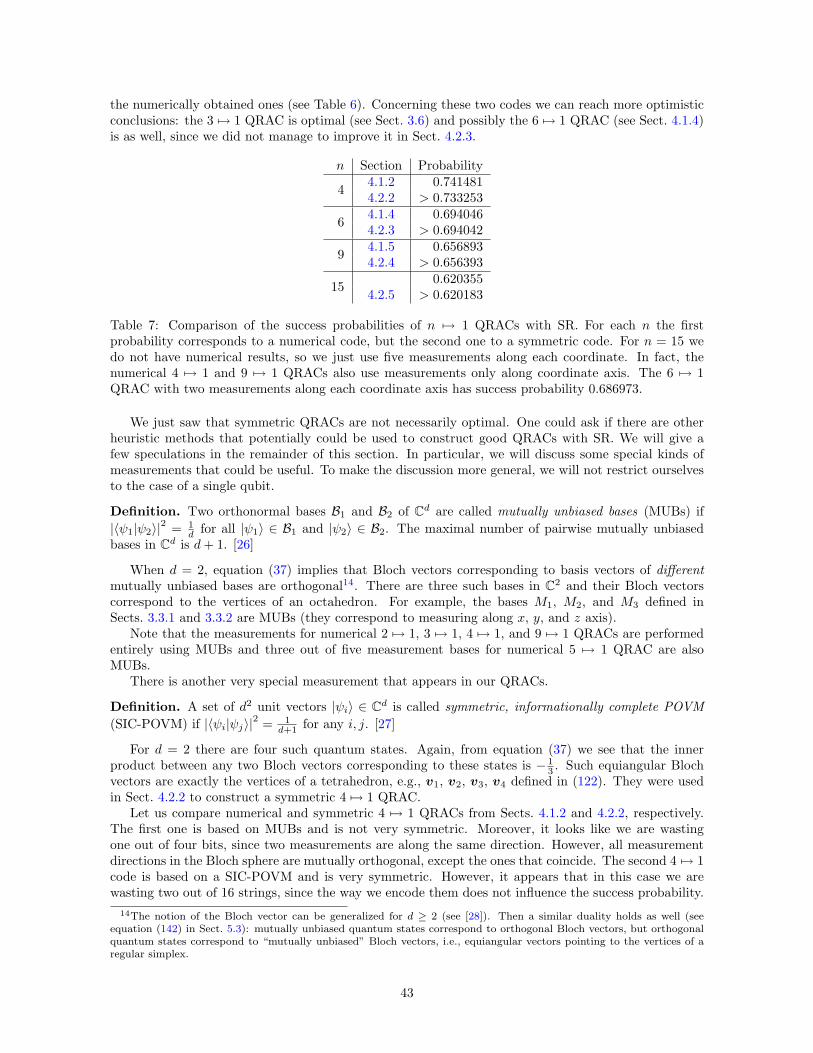
the numerically obtained ones (see Table 6). Concerning these two codes we can reach more optimisticconclusions: the 3 7→ 1 QRAC is optimal (see Sect. 3.6) and possibly the 6 7→ 1 QRAC (see Sect. 4.1.4)is as well, since we did not manage to improve it in Sect. 4.2.3.
n Section Probability
4 4.1.2 0.7414814.2.2 > 0.733253
6 4.1.4 0.6940464.2.3 > 0.694042
9 4.1.5 0.6568934.2.4 > 0.656393
15 0.6203554.2.5 > 0.620183
Table 7: Comparison of the success probabilities of n 7→ 1 QRACs with SR. For each n the firstprobability corresponds to a numerical code, but the second one to a symmetric code. For n = 15 wedo not have numerical results, so we just use five measurements along each coordinate. In fact, thenumerical 4 7→ 1 and 9 7→ 1 QRACs also use measurements only along coordinate axis. The 6 7→ 1QRAC with two measurements along each coordinate axis has success probability 0.686973.
We just saw that symmetric QRACs are not necessarily optimal. One could ask if there are otherheuristic methods that potentially could be used to construct good QRACs with SR. We will give afew speculations in the remainder of this section. In particular, we will discuss some special kinds ofmeasurements that could be useful. To make the discussion more general, we will not restrict ourselvesto the case of a single qubit.
Definition. Two orthonormal bases B1 and B2 of Cd are called mutually unbiased bases (MUBs) if|〈ψ1|ψ2〉|2 = 1
d for all |ψ1〉 ∈ B1 and |ψ2〉 ∈ B2. The maximal number of pairwise mutually unbiasedbases in Cd is d+ 1. [26]
When d = 2, equation (37) implies that Bloch vectors corresponding to basis vectors of differentmutually unbiased bases are orthogonal14. There are three such bases in C2 and their Bloch vectorscorrespond to the vertices of an octahedron. For example, the bases M1, M2, and M3 defined inSects. 3.3.1 and 3.3.2 are MUBs (they correspond to measuring along x, y, and z axis).
Note that the measurements for numerical 2 7→ 1, 3 7→ 1, 4 7→ 1, and 9 7→ 1 QRACs are performedentirely using MUBs and three out of five measurement bases for numerical 5 7→ 1 QRAC are alsoMUBs.
There is another very special measurement that appears in our QRACs.
Definition. A set of d2 unit vectors |ψi〉 ∈ Cd is called symmetric, informationally complete POVM(SIC-POVM) if |〈ψi|ψj〉|2 = 1
d+1 for any i, j. [27]
For d = 2 there are four such quantum states. Again, from equation (37) we see that the innerproduct between any two Bloch vectors corresponding to these states is − 1
3 . Such equiangular Blochvectors are exactly the vertices of a tetrahedron, e.g., v1, v2, v3, v4 defined in (122). They were usedin Sect. 4.2.2 to construct a symmetric 4 7→ 1 QRAC.
Let us compare numerical and symmetric 4 7→ 1 QRACs from Sects. 4.1.2 and 4.2.2, respectively.The first one is based on MUBs and is not very symmetric. Moreover, it looks like we are wastingone out of four bits, since two measurements are along the same direction. However, all measurementdirections in the Bloch sphere are mutually orthogonal, except the ones that coincide. The second 4 7→ 1code is based on a SIC-POVM and is very symmetric. However, it appears that in this case we arewasting two out of 16 strings, since the way we encode them does not influence the success probability.
14The notion of the Bloch vector can be generalized for d ≥ 2 (see [28]). Then a similar duality holds as well (seeequation (142) in Sect. 5.3): mutually unbiased quantum states correspond to orthogonal Bloch vectors, but orthogonalquantum states correspond to “mutually unbiased” Bloch vectors, i.e., equiangular vectors pointing to the vertices of aregular simplex.
43

Now, if we compare the success probabilities of both 4 7→ 1 codes (see Table 7), we see that the firstone is clearly better. Hence we conclude that
orthogonality of the measurement Bloch vectorsseems to be more important than symmetry.
One can come to a similar conclusion when comparing 9 7→ 1 and 15 7→ 1 codes. Thus it looks likeusing roughly n/3 measurements along each coordinate axis is quite a good heuristic for constructingn 7→ 1 QRAC with SR (see Sect. 3.8.2).
5 Conclusion
5.1 Summary
We study the worst case success probability of random access codes with shared randomness. Yao’sprinciple (see equation (5) in Sect. 2.2) and input randomization (see Theorem 1) is applied to considerthe average case success probability instead (this works in both classical and quantum cases).
In Sect. 2.3.2 we construct an optimal classical n 7→ 1 RAC with SR as follows (see Theorem 2):Alice XORs the input string with n random bits she shares with Bob, computes the majority and sendsit to Bob; if the ith bit is requested, Bob outputs the ith bit of the shared random string XORed withthe received bit. The asymptotic success probability of this code is given by equation (27) in Sect. 2.3.2:
p(n) ≈ 12
+1√2πn
. (139)
The worst case success probability of an optimal quantum RAC with SR satisfies the followinginequalities:
12
+
√2
3πn≤ p(n) ≤ 1
2+
12√n. (140)
These upper and lower bounds are obtained in Sects. 3.6 and 3.8.1, respectively.The success probabilities of classical and quantum RACs with SR are compared in Fig. 31.
5.2 Open problems for n 7→ 1 QRACs
Lower bound by orthogonal measurements. The known 2 7→ 1 and 3 7→ 1 QRACs (see Sect. 3.3) andour numerical 4 7→ 1 and 9 7→ 1 QRACs with SR (see Sects. 4.1.2 and 4.1.5) suggest that MUBs can beused to obtain good QRACs (see Sect. 4.3). Indeed, n 7→ 1 QRAC with orthogonal measurements (seeSect. 3.8.2) is better than the one with random measurements (see Sect. 3.8.1). However, we were notable to obtain an asymptotic expression for its success probability. This is equivalent to obtaining anasymptotic expression for (85), i.e., the average distance traveled by a random walk with roughly n/3steps along each coordinate axis.
In Fig. 32 we show how close both lower bounds and the success probabilities of numerical QRACsare relative to the upper bound from Sect. 3.6. Assume that Alice and Bob are given a point in thelight gray region in Fig. 32 and asked to construct a QRAC with SR whose success probability is atleast as good. Then they can use measurements along coordinate axis as in Sect. 3.8.2. If the point isin the dark gray region, they can use one of the numerical codes from Sect. 4.1. However, if it is in thewhite region, they have to solve the next open problem.
Optimality of numerical codes. Prove the optimality of any of the numerically obtained n 7→ 1QRACs with SR for n ≥ 4 discussed in Sect. 4.1. Are the optimal constructions unique (up to isomor-phism)?
Prove the “Homer conjecture” that quantum RACs with SR are at least as good as their classicalcounterparts in the sense discussed at the end of Sect. 3.4.
44

2 3 4 5 6 7 8 9 10 11 12 13 14 15n
0.6
0.7
0.8
0.9
pHnL
Figure 31: Comparison of success probabilities of classical and quantum RACs. Black dots correspondto optimal classical RACs and the dotted line shows the asymptotic behavior. Circles correspond tonumerical QRACs and dashed lines to quantum upper and lower bounds, respectively.
5.3 Possible generalizations
There are several ways that random access codes with SR can be generalized, both classically andquantumly. In particular, one can consider
• n p7→ 1 codes in base d, d > 2 (called qudits in the quantum case),
• n p7→ m codes with m > 1,
• n p7→ m codes where any k > 1 bits (qubits) must be recovered.
Of course, one can consider several of these generalizations simultaneously. In the setting withoutshared randomness such generalizations have already appeared in the literature (see Sect. 1.2). We willbriefly introduce the notion of the generalized Bloch vector which we believe can be useful to studysuch generalizations (it has been explicitly used in [5] to prove the impossibility of 2m
p7→ m QRACwith p > 1/2, when SR is not allowed).
The notion of the Bloch vector introduced in Sect. 3.1.1 can be generalized for d > 2. For example,to write down the density matrix for d = 3 one uses eight Gell-Mann matrices denoted by λi insteadof three Pauli matrices σi defined in equation (35). In general one needs d2 − 1 matrices λi that spanthe set of all traceless d× d Hermitian matrices. A convenient choice of λi are the so called generalizedGell-Mann matrices, also known as the generators of the Lie algebra of SU(d), given in [31]. We canuse them to generalize equation (36):
ρ =1d
(I +
√d(d− 1)
2r · λ
), (141)
45

2 3 4 5 6 7 8 9 10 11 12n
-0.015
-0.010
-0.005
Figure 32: Close-up of the narrow region in Fig. 31 between the quantum upper and lower bound(everything is shown relative to the upper bound that corresponds to the horizontal axis). Circlesindicate the gap between the upper bound and numerical QRACs with SR. Black squares show the gapbetween the upper bound and the lower bound by measurements along coordinate axes (see Fig. 10).Dashed line corresponds to the gap between the quantum upper bound and the lower bound by randommeasurements.
46

where λ = (λ1, . . . , λd2−1) and r ∈ Rd2−1 is the generalized Bloch vector15 or coherence vector [28, 30].Since the λi are chosen so that Trλi = 0 and Tr(λiλj) = 2δij , equation (37) generalizes to
|〈ψ1|ψ2〉|2 = Tr(ρ1ρ2) =1d
(1 + (d− 1) r1 · r2
). (142)
To recover a base d digit, we perform a measurement in an orthonormal basis |ψ1〉 , . . . , |ψd〉 of Cd.Since |〈ψi|ψj〉|2 = 0 for any pair i 6= j, the corresponding Bloch vectors must satisfy ri ·rj = − 1
d−1 . Thismeans that they are the vertices of a regular simplex that belongs to a (d− 1)-dimensional subspaceand is centered at the origin (for d = 2 this is just a line segment).
On the other hand, in Sect. 4.3 we observed that it might be advantageous to perform measurementsalong orthogonal directions in the Bloch sphere to recover different bits. Let ri ⊥ sj be two orthogonalBloch vectors. Then the corresponding quantum states |ψi〉 and |ϕj〉 must satisfy |〈ψi|ϕj〉|2 = 1
d . Thisis exactly the case when |ψi〉 and |ϕj〉 belong to different mutually unbiased bases (see Sect. 4.3).This suggests that distinct bits should be recovered using mutually unbiased measurements. Note thatthe Bloch vectors of the states from two MUBs correspond to the vertices of two regular simplices inmutually orthogonal subspaces. In general, the Bloch vectors of the states from all d+ 1 MUBs are thevectices of the so called complementarity polytope [32], which is just the octahedron when d = 2.
The conclusion of Sect. 4.3 and our discussion above suggests the use of MUBs to construct QRACsalso for d > 2. Such attempts have already been made [6, 8]. Galvao [6] gives an example of 2 0.797−→ 1QRAC for qutrits (d = 3) and Casaccino et al. [8] numerically investigate (d + 1) 7→ 1 QRACs basedon MUBs for d-level quantum systems. However, there is a significant difference between the qubit andqudit case. Recall that for d = 2 the optimal way to encode the message x is to use a unit vector inthe direction of vx (see equation (57) in Sect. 3.4). A similar expression for vx can be obtained whend > 2, but then the matrix ρ assigned to r = vx/ ‖vx‖ according to equation (141) is not necessarilypositive semidefinite and hence may not be a valid density matrix. However, it is known that for smallenough values of ‖r‖ (in our case15 ‖r‖ ≤ 1
d−1 ), all Bloch vectors correspond to valid density matrices[29]. Hence, if we cannot use the pure state corresponding to vx/ ‖vx‖, we can always use the mixedstate corresponding to 1
d−1vx/ ‖vx‖. If one knows more about the shape of the region correspondingto valid quantum states, one can make a better choice and use a longer vector, possibly in a slightlydifferent direction. Unfortunately, apart from convexity, not much is known about this shape. Alreadyfor d = 3 it is rather involved [28, 29]. In general the conditions (in terms of the coordinates of thegeneralized Bloch vector r) for ρ to have non-negative eigenvalues are given in [30, 28].
However, for proving only an upper bound, one can ignore all such details. Thus we believe itmight be possible to generalize our upper bound (see Sect. 3.6 and 3.7) using generalized Bloch vectors.It would be interesting to compare such a result with the upper bound (76) that was obtained byBen-Aroya et al. in [16].
Finally, another way of generalizing QRACs with SR is to add other resources. A good candidateis shared entanglement.
5.4 Acknowledgments
Most of these results were obtained in the summer of 2006 during the undergraduate summer researchprogram at the University of Waterloo. We would like to thank University of Waterloo and IQC for theirhospitality. We would also like to thank Andrew Childs and Ashwin Nayak for many useful commentson the preliminary version of this manuscript. In particular, the simplification of the proof of Lemma 6is due to Ashwin.
A Combinatorial interpretation of sums
In this appendix we give a combinatorial interpretation of the sums in equations (22) and (23) fromSect. 2.3.2. This interpretation is formalized in the form of equations (143) and (144). We referred to
15Our normalization follows [30], where the generalized Bloch sphere has radius 1. Another widely used convention is
to assume radiusp
2(d− 1)/d, e.g., see [28, 29].
47

these equations in Sect. 2.3.2 to obtain an exact formula (26) for the average success probability of anoptimal classical RAC.
Let us consider a set of n distinct elements and count the number of ways to choose more than halfof n elements and mark one of them as special. There are two approaches: first choose the elementsand then mark the special one or first choose the special one and then choose the others.
In the first scenario there are i(ni
)ways to choose exactly i elements and mark one of them as special.
If we have to choose more than half, we obtain the sum∑ni=m+1 i
(ni
)where m =
⌊n2
⌋.
In the second scenario there are n ways to choose the special element. Then there are l = n − 1elements left and at least m of them must be taken to have more than half of n elements in total. Thenumber of ways to do this corresponds to the number of subsets of size at least m of a set of l distinctelements. Let us consider the cases when l is odd and even separately.
If n = 2m then l = 2m − 1 is odd. To each “large” subset of size i (m ≤ i ≤ l) we can assign aunique “small” subset (the complement set) of size l− i (0 ≤ l− i ≤ m−1), and vice versa. Each subsetis either “large” or “small”, so the number of “large” and “small” subsets is the same—it is half of thenumber of all subsets, i.e., 2l/2 = 22m−2.
If n = 2m+1 then l = 2m is even. The “large” subsets have m+1 ≤ i ≤ l elements, but the “small”ones: 0 ≤ l − i ≤ m− 1. Let us call the remaining
(2mm
)subsets of size m “balanced”. In this case the
bijection between the “large” and “small” subsets holds as well, but it maps the “balanced” subsetsto themselves. Thus the total number of all subsets is “large” + “small” +
(2mm
)= 2l. The number of
“large” subsets is(2l +
(2mm
))/2 = 22m−1 + 1
2
(2mm
).
Both counting methods must give the same results, so for odd and even n we obtain, respectively:
2m+1∑i=m+1
i
(2m+ 1
i
)= (2m+ 1) ·
(22m−1 +
12
(2mm
)), (143)
2m∑i=m+1
i
(2mi
)= 2m · 22m−2. (144)
We would like to acknowledge Juris Smotrovs for providing this interpretation.
B POVMs versus orthogonal measurements
An orthogonal (or von Neumann) measurement is not the most general type of measurement of aquantum system. In general a POVM measurement [33, 34] may extract more information. In thisappendix we show that in the qubit case POVMs can be simulated using a probabilistic combination ofenhanced orthogonal measurements, as defined in Sect. 3.7 (such a measurement is either an orthogonalmeasurement or a constant function). To define a POVM we have to introduce the notion of a positivesemidefinite matrix [35].
Definition. A complex square matrix E is called positive semidefinite if 〈ψ|E |ψ〉 ≥ 0 for all |ψ〉.
An equivalent definition is that E is diagonalizable and all eigenvalues of E are real and non-negative.Thus E is Hermitian.
Definition. A positive operator-valued measure (POVM) is a set E1, . . . , Em of positive semidefinitematrices such that
∑mi=1Ei = I. [33, 34]
POVM measurements can have an arbitrary number of outcomes, but in the case of n 7→ 1 QRACswe have to consider only two-outcome single-qubit POVMs. Such a POVM can be specified by E0, E1,where E0 is positive semidefinite and E1 = I − E0. Since E0 is also Hermitian, we can find a basisB = |ψ0〉 , |ψ1〉 in which E0 is diagonal, i.e., E0 =
(a 00 b
). In this basis E1 =
(1−a 00 1−b
). Since both
E0 and E1 are positive semidefinite, 0 ≤ a ≤ 1 and 0 ≤ b ≤ 1. An arbitrary pure qubit state |ψ〉 in the
48

Orthogonal
measurement
p0
p1
0
1
a
1 - a
1 - b
b
0 P0
1 P1
Figure 33: A simulation of the POVM measurement E0, E1 on a qubit using an orthogonal measure-ment and a post-processing of the measurement result.
basis B can be specified by (31). When |ψ〉 is measured, the probabilities of the outcomes areP0 = 〈ψ|E0 |ψ〉 = a cos2
θ
2+ b sin2 θ
2,
P1 = 〈ψ|E1 |ψ〉 = (1− a) cos2θ
2+ (1− b) sin2 θ
2.
(145)
Let us consider the following process (see Fig. 33) that simulates the POVM measurement E0, E1:
1. perform an orthogonal measurement in the basis B = |ψ0〉 , |ψ1〉,
2. perform the following post-processing of the outcome of the measurement:
• if the outcome was 0: output 0 with probability a and output 1 with probability 1− a,
• if the outcome was 1: output 0 with probability b and output 1 with probability 1− b.
To see why this process is equivalent to the POVM measurement E0, E1, consider a pure qubit state|ψ〉 given by (31) in the basis B. When |ψ〉 is measured in the basis B = |ψ0〉 , |ψ1〉, the probabilitiesof the outcomes 0 and 1 are as follows (see also equation (38) in Sect. 3.1.1):
p0 = |〈ψ0|ψ〉|2 = cos2θ
2,
p1 = |〈ψ1|ψ〉|2 = sin2 θ
2.
(146)
Now it is simple to verify that the process shown in Fig. 33 has the same outcome probabilities (145)as the POVM measurement. However, this process is not a probabilistic combination of enhancedorthogonal measurements, since it involves a probabilistic post-processing of the measurement result.To obtain the desired result, we have to modify it. The key idea is that with a certain probability theoutput can be produced without performing an actual measurement.
Let µ = min a, b. Whatever state is input to the process shown in Fig. 33, the probability P0 tooutput 0 is at least µ, because
P0 = p0a+ p1b ≥ (p0 + p1)µ = µ. (147)
Note that µ does not depend on the state being measured. This means that one can output 0 withprobability µ without performing an actual measurement. A similar lower bound holds for P1 as well:
P1 = p0(1− a) + p1(1− b) ≥ (p0 + p1)(1−M) = 1−M, (148)
where M = max a, b = a + b − µ. Let us consider the following probabilistic combination of fourdecoding strategies:
• with probability c0: output 0 without performing a measurement,
49

• with probability c1: output 1 without performing a measurement,
• with probability c01: measure in the basis |ψ0〉 , |ψ1〉,
• with probability c10: measure in the opposite basis |ψ1〉 , |ψ0〉.
The resulting probabilities of outcomes for this process areP0 = c0 + c01p0 + c10p1,
P1 = c1 + c01p1 + c10p0.(149)
We can use the lower bounds (147) and (148) for P0 and P1, respectively, to assign the probabilities c0,c1, c01, and c10 in the following way:
c0 = µ,
c1 = 1− (a+ b) + µ,
c01 = a− µ,c10 = b− µ
(150)
(note that at least one of the probabilities c01 or c10 will be zero). It is not hard to verify that after theassignment (150) the probabilities P0 and P1 in (149) will match the probabilities of outcomes (145) ofthe POVM measurement.
Thus for each qubit POVM given by a and b one can find a probabilistic combination of enhancedorthogonal measurements given by c0, c1, c01, and c10, such that in both cases the probabilities ofoutcomes are the same.
Example. For a = b = 1/2 we have c0 = c1 = 1/2 and c01 = c10 = 0, corresponding to randomguessing (observe that E0 = E1 in this case).
Example. However, a = 1 and b = 0 corresponds to a projective measurement in basis |ψ0〉 , |ψ1〉,because c01 = 1 and c10 = c0 = c1 = 0.
Example. Finally, a = 1 and b = 1 corresponds to a constant function 0, because c0 = 1 andc01 = c10 = c1 = 0.
References
[1] Stephen Wiesner, “Conjugate coding,” SIGACT News, vol. 15, issue 1, pp. 78–88, 1983.
[2] Andris Ambainis, Ashwin Nayak, Amnon Ta-Shma, Umesh Vazirani, “Dense quantum coding anda lower bound for 1-way quantum automata,” Proceedings of the 31st Annual ACM Symposiumon Theory of Computing (STOC’99), pp. 376–383, 1999. arXiv:quant-ph/9804043v2
[3] Andris Ambainis, Ashwin Nayak, Amnon Ta-Shma, Umesh Vazirani, “Dense Quantum Coding andQuantum Finite Automata,” Journal of the ACM, vol. 49, no. 4, pp. 496–511, 2002.
[4] Ashwin Nayak, “Optimal lower bounds for quantum automata and random access codes,” Proceed-ings of the 40th IEEE Symposium on Foundations of Computer Science (FOCS’99), pp. 369–376,1999. arXiv:quant-ph/9904093v3
[5] Masahito Hayashi, Kazuo Iwama, Harumichi Nishimura, Rudy Raymond, Shigeru Yamashita,“(4, 1)-Quantum Random Access Coding Does Not Exist,” New J. Phys., vol. 8, no. 8, pp. 129,2006. arXiv:quant-ph/0604061v1
[6] Ernesto F. Galvao, “Foundations of quantum theory and quantum information applications,” PhDthesis, University of Oxford, 2002.
50

[7] Robert W. Spekkens, Daniel H. Buzacott, Anthony J. Keehn, Ben Toner, Geoff J. Pryde, “Prepara-tion contextuality powers parity-oblivious multiplexing,” Phys. Rev. Lett., vol. 102, no. 1, 010401,2009. arXiv:0805.1463v2
[8] Andrea Casaccino, Ernesto F. Galvao, Simone Severini, “Extrema of discrete Wigner functionsand applications,” Phys. Rev. A 78, 022310, 2008. arXiv:0805.3466v2
[9] Hartmut Klauck, “Lower bounds for quantum communication complexity,” Proceedings of the42nd IEEE Symposium on Foundations of Computer Science (FOCS’01), pp. 288, 2001.arXiv:quant-ph/0106160v3
[10] Scott Aaronson, “Limitations of Quantum Advice and One-Way Communication,” Proceedings ofthe 19th Annual IEEE Conference on Computational Complexity (CCC’04), pp. 320–332, 2004.arXiv:quant-ph/0402095v4
[11] Dmitry Gavinsky, Julia Kempe, Oded Regev, Ronald de Wolf, “Bounded-Error Quantum StateIdentification and Exponential Separations in Communication Complexity,” Proceedings of the38th Annual ACM Symposium on Theory of Computing (STOC’06), pp. 594–603, 2006.arXiv:quant-ph/0511013v1
[12] Masahito Hayashi, Kazuo Iwama, Harumichi Nishimura, Rudy Raymond, Shigeru Yamashita,“Quantum Network Coding,” Proceedings of the 24th International Symposium on TheoreticalAspects of Computer Science (STACS’07), pp. 610–621, 2007. arXiv:quant-ph/0601088v2
[13] Iordanis Kerenidis, “Quantum Encodings and Applications to Locally Decodable Codes and Com-munication Complexity,” PhD thesis, University of California at Berkeley, 2004.
[14] Iordanis Kerenidis, Ronald de Wolf, “Exponential Lower Bound for 2-Query Locally DecodableCodes via a Quantum Argument,” J. Comput. Syst. Sci., vol. 69, 3, pp. 395–420, 2004.arXiv:quant-ph/0208062v2
[15] Stephanie Wehner, Ronald de Wolf, “Improved Lower Bounds for Locally Decodable Codes andPrivate Information Retrieval,” Automata, Languages and Programming, pp. 1424–1436, 2005.arXiv:quant-ph/0403140v2
[16] Avraham Ben-Aroya, Oded Regev, Ronald de Wolf, “A Hypercontractive Inequality for Matrix-Valued Functions with Applications to Quantum Computing and LDCs,” Proceedings of the 49thAnnual IEEE Symposium on Foundations of Computer Science (FOCS’08), pp. 477–486, 2008.arXiv:0705.3806v2
[17] Scott Aaronson, “The Learnability of Quantum States”, Proc. Roy. Soc. London Ser. A, vol. 463,no. 2088, pp. 3089–3114, 2007. arXiv:quant-ph/0608142v3
[18] Andrew Chi-Chin Yao, “Probabilistic computations: Toward a unified measure of complexity,”Proceedings of the 18th Annual IEEE Symposium on Foundations of Computer Science (SFCS’77),pp. 222–227, 1977.
[19] Giuliano Benenti, Giulio Casati, Giuliano Strini, “Principles of Quantum Computation and Infor-mation,” vol. 1, World Scientific, 2004.
[20] Eric W. Weisstein, “Stirling’s Approximation,” MathWorld.http://mathworld.wolfram.com/StirlingsApproximation.html
[21] Eric W. Weisstein, “Sphere Point Picking,” MathWorld.http://mathworld.wolfram.com/SpherePointPicking.html
[22] Subrahmanyan Chandrasekhar, “Stochastic Problems in Physics and Astronomy,” Reviews of Mod-ern Physics, vol. 15, no. 1, 1943.
[23] Barry D. Hughes, “Random Walks and Random Environments,” vol. 1, Clarendon Press, 1995.
51

[24] Larry C. Grove, Clark T. Benson, “Finite Reflection Groups”, 2nd Ed., Springer, 1985.
[25] Walter W. Rouse Ball, H.S.M. Coxeter, “Mathematical Recreations and Essays,” 13th Ed., CourierDover Publications, 1987.
[26] William K. Wootters, Brian D. Fields, “Optimal State-Determination by Mutually Unbiased Mea-surements,” Annals of Physics, vol. 191, Issue 2, pp. 363–381, 1989.
[27] Joseph M. Renes, Robin Blume-Kohout, Andrew J. Scott, Carlton M. Caves, “Symmetric Infor-mationally Complete Quantum Measurements,” J. Math. Phys., vol. 45, pp. 2171–2180, 2004.arXiv:quant-ph/0310075v1
[28] Gen Kimura, “The Bloch vector for N-level systems,” Physics Letters A, vol. 314, Issues 5–6,pp. 339–349, 2003. arXiv:quant-ph/0301152v2
[29] Gen Kimura, Andrzej Kossakowski, “The Bloch-Vector Space for N-Level Systems: the Spherical-Coordinate Point of View,” Open Syst. Inf. Dyn., vol. 12, no. 3, pp. 207–229, 2005.arXiv:quant-ph/0408014v2
[30] Mark S. Byrd, Navin Khaneja, “Characterization of the Positivity of the Density Matrix in Termsof the Coherence Vector Representation,” Phys. Rev. A, vol. 68, Issue 6, 062322, 2003.arXiv:quant-ph/0302024v2
[31] Foek T. Hioe, Joseph H. Eberly, “N-Level Coherence Vector and Higher Conservation Laws inQuantum Optics and Quantum Mechanics,” Phys. Rev. Lett., vol. 47, pp. 838–841, 1981.
[32] Ingemar Bengtsson, Asa Ericsson, “Mutually Unbiased Bases and the Complementarity Polytope,”Open Syst. Inf. Dyn., vol. 12, no. 2, pp. 107–120, 2005. arXiv:quant-ph/0410120v1
[33] Michael A. Nielsen, Isaac L. Chuang, “Quantum Computation and Quantum Information,” Cam-bridge University Press, 2000.
[34] Asher Peres, “Quantum Theory: Concepts and Methods,” Kluwer Academic Publishers, 2002.
[35] Roger A. Horn, Charles R. Johnson, “Matrix Analysis,” Cambridge University Press, 1985.
52