Quantum Recurrent Networks for Simulating Stochastic Processes

Michail Zak’ & Colin P. Williams*

Ultracomputing Group, Mail Stop 126-347, Jet Propulsion Laboratory. California Institute of Technology. Pasadena, CA 91 109-8099

colin@solstice.jpl.naa.gov, zak@solstice.jpl.nasa.gov

Abstract. We introduce the concept of quantum recurrent networks by incorporating classical feedback loops into conventional quantum networks. We show that the dy- namical evolution of such networks, which interleave quantum evolution with meas- urement and reset operations, exhibit novel dynamical properties finding application in pattern recognition, optimization and simulation. Moreover, decoherence in quantum recurrent networks is less problematic than in conventional quantum net- work architectures due to the modest phase coherence times needed for network op- eration.

Introduction

Large scale classical simulations of stochastic processes require vast quantities of random numbers. However, since the pioneering work of Church, Turing, Post and G a e l , it has been known that classical computers can only computefuncrions. In other words, the class of tasks that can be accomplished with a classical computer is exactly equivalent to the class of computable functions. However, as there is nofuncrion for computing a true ran- dom number, classical computers can only feign randomness. The purported calls to the “random number generator” often seen in modem programming languages are, in reality, calls to a pseudo-random number generator. A pseudo-random number generator is a deterministic function whose successive outputs pass many of the statistical tests of ran- domness. Unfortunately, the sequence of outputs can also harbor subtle correlations that are not immediately apparent from the common statistical measures of randomness.

Supported by the JPL Information and Computing Technologies Research Section. Supported by the NASNJPL Center for Integrated Space Microsystems and by the JPL Informa- tion and Computing Technologies Research Section.

2 Michail Zak and Colin P. Williams

To illustrate this point vividly, consider the RANDU “linear congruential genera- tor”, a notoriously bad pseudo-random number generator that was common on IBM main- frames of the 1960s. A linear congruential generator is defined by:

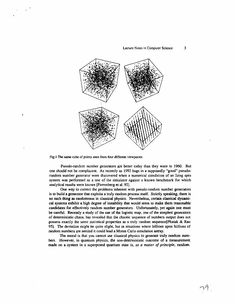
N k + , = ( C N , +m) mod n where I , m, n are fixed integers and k = 1.2.3, ... The resulting sequence of numbers, appears, superficially, to generate a set of random samples from a uniform distribution that lie in the range 0 to n - 1 inclusive. We say “superficially” in the sense that, the sequence of numbers N , , N , , ... p asses many statistical tests of randomness. However, there is a subtle correlation lurking amongst these numbers that becomes apparent if you use them to choose a set of (supposedly) random points in a high dimensional space. In particular, if, as in RANDU, C = 65539, n = 2”. m = 0 and N o = 1 then successive triples produced by the generator, N , , N,, , , Nk+* , can be taken to define the x-, y - and z-coordinates of a point in a 3-dimensional space. These points are plotted in fig.1 below from different viewing angles. From most viewing angles the points appear to be randomly distributed. But from a particular viewing angle you can see that they are not at all randomly distrib- uted. In fact they lie in a set of parallel planes. Thus the sequence of supposedly “random” numbers output from the linear congruential generator are not random at all and could give misleading results if used in a numerical simulation of a stochastic process.

Lecture Notes in Computer Science 3

Fig. 1 The same cube of points seen from four different viewpoints

Pseudo-random number generators are better today than they were in 1960. But one should not be complacent. As recently as 1992 bugs in a supposedly "good" pseudo- random number generator were discovered when a numerical simulation of an Ising spin system was performed as a test of the simulator against a known benchmark for which analytical results were known [Ferrenberg et ai. 921.

One way to correct the problems inherent with pseudo-random number generators is to build a generator that exploits a truly random process itself. Strictly speaking, there is no such thing as randomness in classical physics. Nevertheless, certain classical dynami- cal systems exhibit a high degree of instability that would seem to make them reasonable candidates for effectively random number generators. Unfortunately, yet again one must be careful. Recently a study of the use of the logistic map, one of the simplest generators of deterministic chaos, has revealed that the chaotic sequence of numbers output does not possess exactly the same statistical properties as a truly random sequence[Phatak & Rao 951. The deviation might be quite slight, but in situations where billions upon billions of random numbers are needed it could lead a Monte Carlo simulation astray.

The moral is that you cannot use classical physics to generate truly random num- bers. However, in quantum physics, the non-deterministic outcome of a measurement made on a system in a superposed quantum state is, us u murrer of principle, random.

4 Michail Zak and Colin P. Williams

Unfortunately, quantum non-determinism is generally regarded as being of lesser impor- tance than other quantum phenomena such as quantum interference and entanglement. This is partly because many people believe, mistakenly, that pseudo-random number gen- erators are “good enough” and partly because the impressive speedups exhibited by quan- tum algorithms for factoring composite integers and for finding an item in an unsorted database, are due to interference and entanglement effects rather than non-determinism. However, such a dismissal of quantum non-determinism is premature. No matter how good new pseudo-random number generators are purported to be, their adequacy can only be assessed empirically within the context of a specific application. Moreover, the key quantum effect on which quantum cryptography depends is quantum non-determinism. We argue that as quantum non-determinism is, intrinsically, a random process, it provides a much better basis for the design of a random number generator.

It is easy to define a quantum procedure for selecting random integers in the range 0 to 2” - 1 by preparing n qubits in the state I O>lO>(O)..-I 0) , applying the Walsh- Hadamard transform to each qubit separately, creating an equal superposition of all possi- ble states of the register, and then reading the memory register. Once you have a mecha- nism for generating uniformly distributed random numbers you can create a generator for any other distribution using a function transformation[Tuckwell95].

However true random number generation is not the same as true stochastic process generation. For example, in a Markov process the probability of obtaining a particular outcome for the next state depends upon the identity of the last state visited. By contrast the sequence of outcomes from a quantum random number generator are independent, identically distributed random variables. It is therefore interesting to ask whether there is a more direct way of using quantum mechanics to simulate stochastic processes?

Quantum Recurrent Networks

We can begin be asking what general features must such a simulator possess? First, we need to be able to generate a sequence of classically observable samples. This suggests that we are going to have to imagine a quantum device that allows repeated measurements. Second, we need to be able bias the probability that a given state will appear as the next output given knowledge of some or all of the previous outputs. This is because, by defini- tion, stochastic processes possess such a memory effect. The simplest way to accommo- date such a memory effect is to imagine that the device is reset in a new state that some- how takes account of the states visited so far. These considerations lead naturally to our notion of a “quantum recurrent network”.

A quantum recurrent network consists of a conventional quantum network aug- mented with a classical measurement and quantum reset operation. The design of a one dimensional quantum recurrent network is shown in Fig.2.

Lecture Notes in Computer Science 5

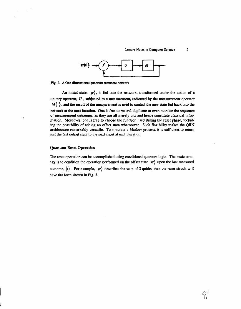
Fig. 2. A One dimensional quantum recurrent network

An initial state, Iw), is fed into the network, transformed under the action of a unitary operator, U , subjected to a measurement, indicated by the measurement operator M { } , and the result of the mequrement is used to control the new state fed back into the

network at the next iteration. One is free to record, duplicate or even monitor the sequence of measurement outcomes, as they are all merely bits and hence constitute classical infor- mation. Moreover, one is free to choose the function used during the reset phase, includ- ing the possibility of adding no offset state whatsoever. Such flexibility makes the QRN architecture remarkably versatile. To simulate a Markov process, it is sufficient to return just the last output state to the next input at each iteration.

Quantum Reset Operation

The reset operation can be accomplished using conditional quantum logic. The basic strat- egy is to condition the operation performed on the offset state I v) upon the last measured

outcome, 1'). For example, I v) describes the state of 3 qubits. then the reset circuit will have the form shown in Fig. 3.

s!

6 Michail Zak and Colin P. Williams

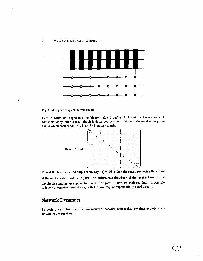
Fig. 3. Most general quantum reset circuit.

Here, a white dot represents the binary value 0 and a black dot the binary value 1. Mathematically, such a reset circuit is described by a 64 X 64 block diagonal unitary ma- trix in which each block, Si , is an 8 x 8 unitary matrix.

. . . . . . . . . . . . . ( s o ; : : : : : :

i s , ; ; I ; j ; j js,i i i i i

is, i i i :

: : : : is,; i : : : : I ;s,i

\ . . . . i i is,

.... ..>.....A" .. ..: ..... ".r. .... .:.. .. ..; ...... L.. .. . . . . . .

...... C . . ... .) ......("." .. >. ..... < ...... + ...... )."" . . . . . ......_... ............................ ....-............ . . . . . . . . . . .

Reset Circuit .... ..i.. .... .i ...... ,. ............. .,_. .... .< ...... ,- .... .............. .... ._, ..... __:.. ..?..; .... ...i ...... i... .. : : : I S : . .

. . . * . I * . . . . . * .

. . . . . . . . . . . .... .."" .......... 2. .... ..L. .......... ..- ............ . . . . . . . . . . . . . .... ..& .... .) ...... + .... "i. .... -;" .... + ...... ). .... . . . . . . . . . . . . . .

Thus if the last measured output were. say, I i ) = IO1 1) then the state re-entering the circuit

at the next iteration will be S,l y ) . An unfortunate drawback of the reset scheme is that the circuit contains an exponential number of gates. Later, we shall see that it is possible to invent alternative reset strategies that do not require exponentially sized circuits.

Network Dynamics

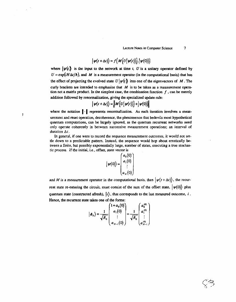
By design, we imbue the quantum recurrent network with a discrete time evolution ac- cording to the equation:

Lecture Notes in Computer Science 7

1

where Ir(r) is the input to the network at time r, U is a unitary operator defined by U = exp(iHAf/h), and M is a measurement operator (in the computational basis) that has the effect of projecting the evolved state U I V(r) into one of the eigenvectors of M . The curly brackets are intended to emphasize that M is to be taken as a measurement opera- tion not a matrix product. In the simplest case, the combination function f , can be merely addition followed by renormalization, giving the specialized update rule:

i w c ~ . a t ) ) = ) ~ { ~ l . ( ~ ) ) } + l ~ O ) ~ ~

where the notation 1 1 represents renormalization. As each iteration involves a meas- urement and reset operation, decoherence, the phenomenon that bedevils most hypothetical quantum computations, can be largely ignored, as the quantum recurrent networks need only operate coherently in between successive measurement operations; an interval of duration A t .

In general, if one were to record the sequence measurement outcomes, it would not set- tle down to a predictable pattern. Instead, the sequence would hop about erratically be- tween a finite, but possibly exponentially large, number of states, executing a true stochas- tic process. If the initial, i.e., offset, state vector is

and M is a measurement operator in the computational basis, then I ~ ( t + Af)) , the recur-

rent state re-entering the circuit, must consist of the sum of the offset state, I ~ ( 0 ) ) plus

quantum state (constructed afresh), l i) , that corresponds to the last measured outcome, i . Hence, the recurrent state takes one of the forms:

(as ’

8 Michail Zak and Colin P. Williams

"

' N - l ( O ) )

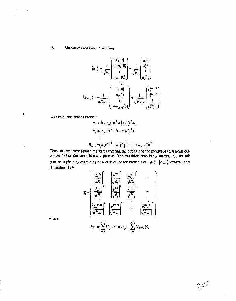
with re-normalization factors: Ro =Il+u,,(O] 2 + I uI(O)1'+ ...

I?, "uo(0)~' +II+a,(O)('+...

RN-1 =la,(O]' + 1 ~ 1 ( 0 ) ( 2 . . . ~ l + ~ N - , ( O ~ ' Thus, the recurrent (quantum) states entering the circuit and the measured (classical) out- comes follow the Same Markov process. The transition probability matrix, q , for this process is given by examining how each of the recurrent states, I m ) . . . I q 5 + , ) evolve under the action of U:

T , =

...

...

where N - l N - 1

Lecture Notes in Computer Science 9

1

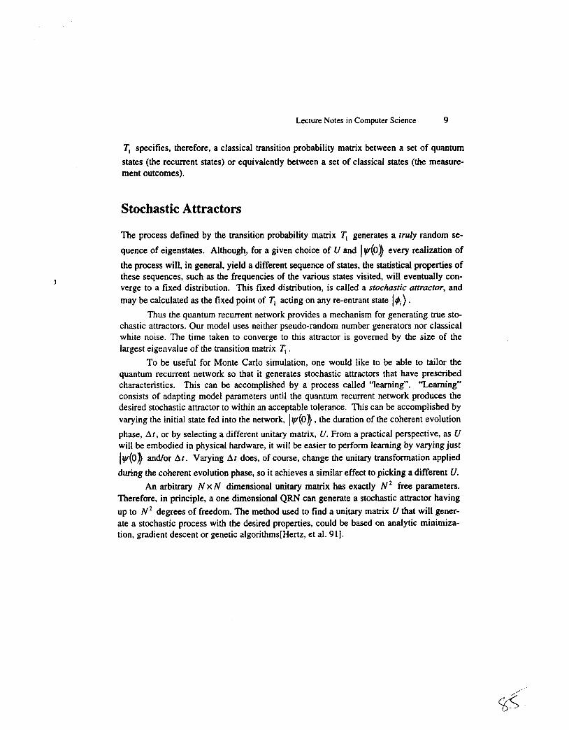
7’, specifies, therefore, a classical transition probability matrix between a set of quantum states (the recurrent states) or equivalentiy between a set of classical states (the measure- ment outcomes).

Stochastic Attractors

The process defined by the transition probability matrix T, generates a trufy random se- quence of eigenstates. Although, for a given choice of U and Iy(0) every realization of the process will, in general, yield a different sequence of states, the statistical properties of these sequences, such as the frequencies of the various states visited, will eventually con- verge to a fixed distribution. This fixed distribution, is called a stochastic utfructor, and may be calculated as the fixed point of T, acting on any re-entrant state lei).

Thus the quantum recurrent network provides a mechanism for generating true sto- chastic attractors. Our model uses neither pseudo-random number generators nor classical white noise. The time taken to converge to this attractor is governed by the size of the largest eigenvalue of the transition matrix .

To be useful for Monte Carlo simulation, one would like to be able to tailor the quantum recurrent network so that it generates stochastic attractors that have prescribed characteristics. This can be accomplished by a process called “learning”. “Learning” consists of adapting model parameters until the quantum recurrent network produces the desired stochastic attractor to within an acceptable tolerance. This can be accomplished by varying the initial state fed into the network, Iy1(0>>, the duration of the coherent evolution phase, A t , or by selecting a different unitary matrix, U. From a practical perspective, as U will be embodied in physical hardware, it will be easier to perform learning by varying just lv(O>) and/or Ar. Varying A t does, of course, change the unitary transformation applied during the coherent evolution phase, so it achieves a similar effect to picking a different U.

An arbitrary N x N dimensional unitary matrix has exactly N 2 free parameters. Therefore, in principle, a one dimensional QRN can generate a stochastic attractor having up to N 2 degrees of freedom. The method used to find a unitary matrix U that will gener- ate a stochastic process with the desired properties, could be based on analytic minimiza- tion, gradient descent or genetic algorithms[Hertz, et al. 91 I.

Lecture Notes in Computer Science 1 1

1

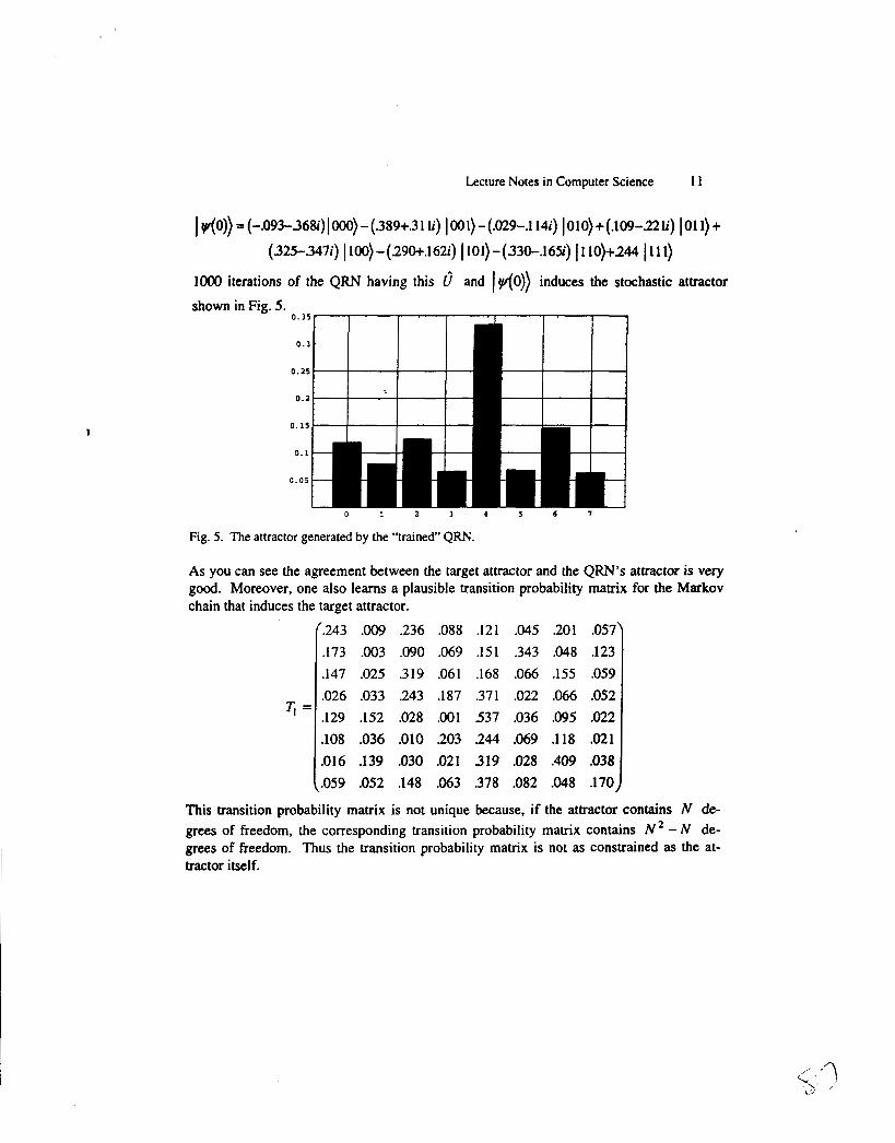
~y(O))=(-.O93-368i)~OOO)-(.389+.311i) IOOl)-(.O29-.114i) (010)+(.109-221i) loll)+

(325-371') 1100)-(290+.162i) 1101)-(330-.16Si) 1110)+244 1111)

IO00 iterations of the QRN having this and I do)) induces the stochastic attractor

shown in Fig. 5. ""

0 . 3

0.1s

0 . 2

0 . 1 5

0 . 1

0 . 0 5

0 1 2 3 4 5 6 7

Fig. 5. The attractor generated by the "trained" QRN.

As you can see the agreement between the target attractor and the QRN's attractor is very good. Moreover, one also learns a plausible transition probability matrix for the Markov chain that induces the target attractor.

.243 .009 .236

.I73 .003 .090

.147 .025 .319

.026 .033 .243

.129 .152 .028 S O 8 .036 .010 .OI6 .I39 .030 .059 .052 .I48

.088 .121 .045

.069 .151 .343

.061 .168 .066

.187 .371 .022

.001 537 .036

.203 .244 .069

.021 319 .028

.063 .378 .082

201 .057 .048 .I23 .155 .059 ,066 .052 .095 . a 2 .118 .021 .409 .038 .048 .I70

This transition probability matrix is not unique because, if the attractor contains N de- grees of freedom, the corresponding transition probability matrix contains N 2 - N de- grees of freedom. Thus the transition probability matrix is not as constrained as the at- tractor itself.

10 Michail Zak and Colin P. Williams

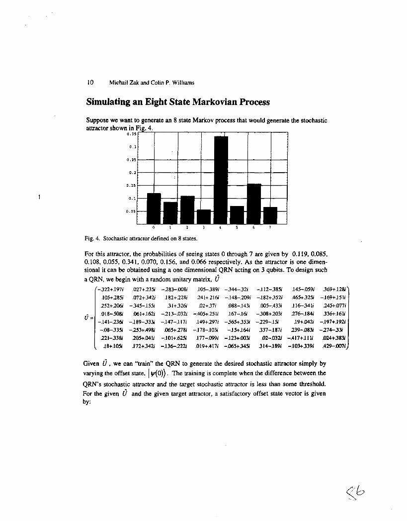
Simulating an Eight State Markovian Process

Suppose we want to generate an 8 state Markov process that would generate the stochastic attractor

Fig. 4. Stochastic attractor defined on 8 states.

For this attractor, the probabilities of seeing states 0 through 7 are given by 0.1 19.0.085, 0.108, 0.055, 0.341, 0.070, 0.156. and 0.066 respectively. As the attractor is one dimen- sional it can be obtained using a one dimensional QRN acting on 3 qubits. To design such a QRN, we begin with a random unitary matrix, C

/-322+.197i .027+.235i -283-.008i .105-389i -344-,321’ -.I 12-385 .145-.059i 369+.12% .105+285i .072+.342i .182+.228i .241+.216i -.148-.209i -.182+352i .465+325i -.169+.151i 252+206’ -345-.155i 31+326i .02+37i .088-.143i .005-.433i .I 16-341i 245tM7i .018-50% .061+.162i -213-.032i -.405+25li .167-.16i -308+203i 276.1841’ 336+.16li

-.141-238 -.189-333i -.147-.I 17i .149+.297i -565+353i -229-.15i .19+.042i -.197+.192i -.08-335i -253+.498i .065+.278i -.178-.103i -.15+.164i 337-.187i 239-.083 -274-33 221-33% 205t.041i -.101+.625i .177-.0991’ -.123+.003i .02-.032i -.417+.l1 li .024+383 , .18+.105i .l72+342i -.136-.222i .019+.417i -.065+345i 314-.189i -.103+339i AB-Mni,

6 =

Given f i , we can “train” the QRN to generate the desired stochastic attractor simply by varying the offset state, I y(0)). The training is complete when the difference between the

QRN’s stochastic attractor and the target stochastic attractor is less than some threshold. For the given C and the given target attractor, a satisfactory offset state vector is given by:

12 Michail Zak and Colin P. Williams

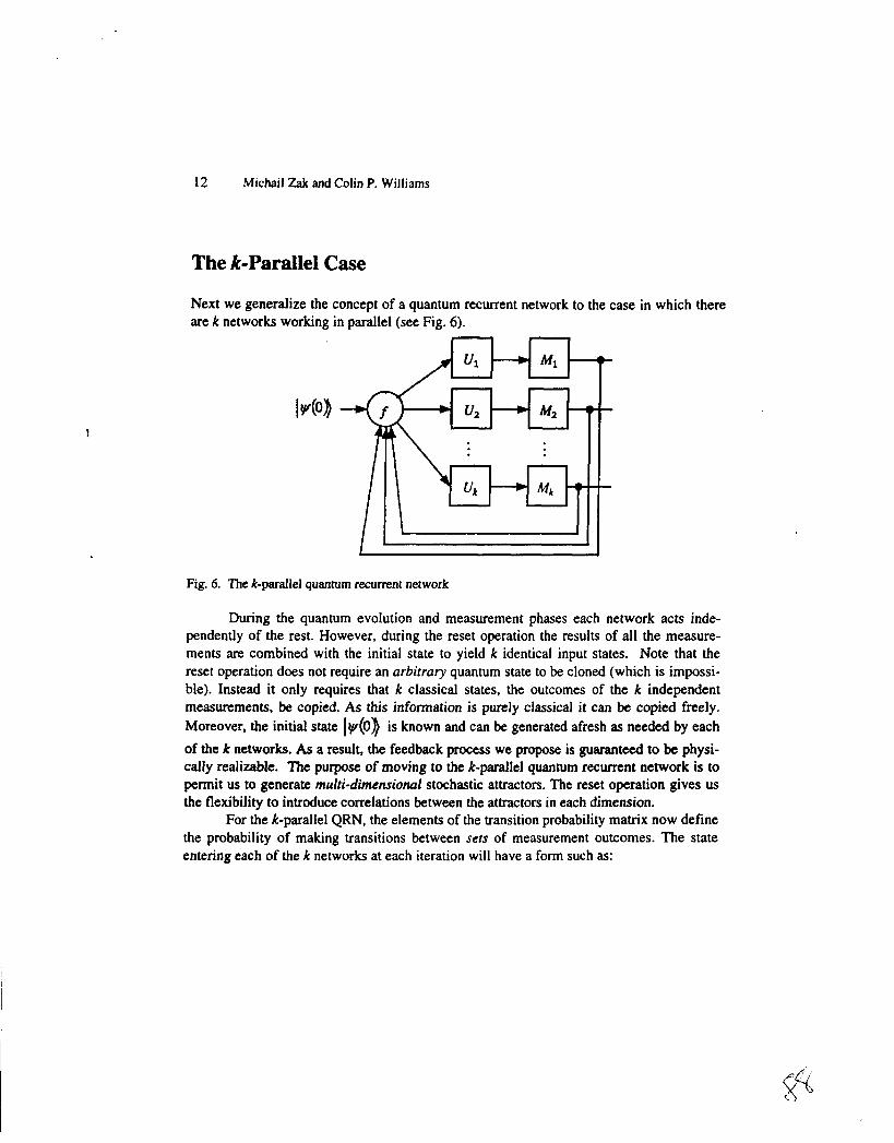
The k-Parallel Case

Next are k

we generalize the concept of a quantum recurrent network to the case networks working in parallel (see Fig. 6).

in which there

Fig. 6. The k-parallel quantum recurrent network

During the quantum evoIution and measurement phases each network acts inde- pendently of the rest. However, during the reset operation the results of all the measure- ments are combined with the initial state to yield k identical input states. Note that the reset operation does not require an arbitrary quantum state to be cloned (which is impossi- ble). Instead it only requires that k classical states, the outcomes of the k independent measurements, be copied. As this information is purely classical it can be copied freely. Moreover, the initial state Iw(0) is known and can be generated afresh as needed by each of the k networks. As a result, the feedback process we propose is guaranteed to be physi- cally realizable. The purpose of moving to the k-parallel quantum recurrent network is to permit us to generate mulri-dimensional stochastic attractors. The reset operation gives us the flexibility to introduce correlations between the attractors in each dimension.

For the k-parallel QRN, the elements of the transition probability matrix now define the probability of making transitions between sets of measurement outcomes. The state entering each of the k networks at each iteration will have a form such as:

Lecture Notes in Computer Science 13

1

1

where the sequence ili, ... it specifies the last ordered set of measurement outcomes ob- tained from the k networks and Rk.. j k is the renormalization constant given by:

The mathematical form of the Aplitude depends upon how many of the com- ponents in the k-parallel network produced the same measurement outcome at the last iteration through the QRN i.e. how many of the i , , in the sequence i l i , . . . i , were the

same. If outcome it is obtained nit times we have = nit +a, (0).

As there are k networks and each network can produce one of N outcomes (independently), the k-parallel transition matrix defines a mapping from N‘ distinct sets of input states to N‘ sets of output states. If we denote the probability of transitioning from the set of inputs ili2 ... ik to the set of outputs j l j t ... j t by p:::;’ we have:

A . ..lt

where

Thus the k-parallel transition probability matrix has a tensor structure of the form = b:;:::: kl,, where the sequences ili2 ... it and j l j z . . . j , are defined with respect

to some consistent ordering. For the k-parallel architecture, there are k N’ free parameters. Thus we ought to be able

to generate k-dimensional stochastic attractors having up to k N 2 degrees of freedom. An interesting corollary of the QRN dynamics concerns the dynamical behavior of

two k=l QRNs in comparison to a single k=2 QRN that combines them both. For simplic- ity we can set the initial (offset) state vector Iv/(O>> to be zero. Considered separately, the

resulting stochastic processes have transition probabilities p: ) and p;:’ given by:

14 Michail Zak and Colin P. Williams

By contrast the transition probability matrix of the joint QRN has components:

Clearly p:;:) f p:) x p:' in general. Thus the two dimensional stochastic attractor gen-

erated by a 2-parallel quantum. recurrent network is not simply the product of two 1- dimensional stochastic attractors.

Alternative Reset Strategies

So far, we have described the most general quantum recurrent network, i.e., one which involves an arbitrary offset state and an arbitrary unitary operator. Unfortunately, for such QRNs, the reset operation requires a circuit, like that depicted in Fig. 3, which is exponential in the number of qubits. This is because the required reset is different de- pending on which of the 2" possible outcomes was obtained at the last measurement. Moreover, to implement an arbitrary unitary matrix as a quantum circuit could, in the worst case, require an exponential number of quantum gates[Knill 951. Both these short- comings can be sidestepped, however, by a slight modification to the QRN.

Instead of allowing any multi-particle state vector to serve as the offset vector we could allow only product states. This would enable the reset operation to be achieved in only a polynomial number of operations. For example, suppose the offset vector for a 2- qubit QRN is the product state I y ) , 1 @)2, then, instead of the reset operation with expo-

nential cost, i.e., if a and b are the most recently measured classical outcomes,

lv),l42 - l l I v ) , l 4 2 + I u), I b)2 11 , we could impose a qubit-by-qubit reset operation

Iw),le)2 H I I (Iv), +1a),)(1#)2 +lb)211. Although the latter operation is conditional

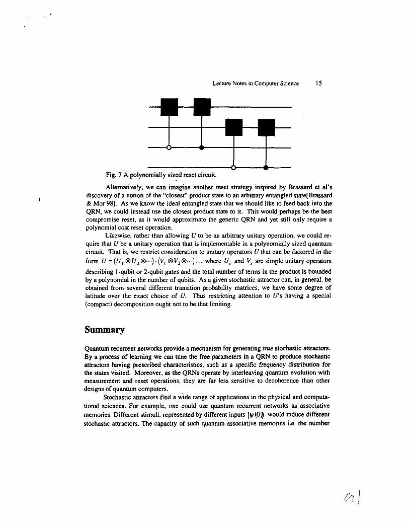
too, the conditioning is with respect to each individual qubit rather than the state of the entire multi-qubit register. Thus, the polynomial cost reset circuit would have the form shown in Fig. 7.

Lecture Notes in Computer Science 15

Fig. 7 A polynomially sized reset circuit.

Alternatively, we can imagine another reset strategy inspired by Brassard et al’s discovery of a notion of the “closest” product state to an arbitrary entangled state[Brassard & Mor 981. As we know the ideal entangled state that we should like to feed back into the QRN, we could instead use the closest product state to it. This would perhaps be the best compromise reset, as it would approximate the generic QRN and yet still only require a polynomial cost reset operation.

Likewise, rather than allowing U to be an arbitrary unitary operation, we could re- quire that U be a unitary operation that is implementable in a polynomially sized quantum circuit. That is, we restrict consideration to unitary operators (I that can be factored in the form U = ( U , @Uu,@. . . ) . (V, @V,@‘.) ... where U i and Vi are simple unitary operators describing I-qubit or 2-qubit gates and the total number of terms in the product is bounded by a polynomial in the number of qubits. As a given stochastic attractor can, in general, be obtained from several different transition probability matrices, we have some degree of latitude over the exact choice of U. Thus restricting attention to U s having a special (compact) decomposition ought not to be that limiting.

Summary

Quantum recurrent networks provide a mechanism for generating true stochastic attractors. By a process of learning we can tune the free parameters in a QRN to produce stochastic attractors having prescribed characteristics, such as a specific frequency distribution for the states visited. Moreover, as the QRNs operate by interleaving quantum evolution with measurement and reset operations, they are far less sensitive to decoherence than other designs of quantum computers.

Stochastic attractors find a wide range of applications in the physical and computa- tional sciences. For example, one could use quantum recurrent networks as associative memories. Different stimuli, represented by different inputs 1~ [ O ) would induce different stochastic attractors. The capacity of such quantum associative memories i.e. the number

16 Michail Zak and Colin P. Williams

of distinct stimuli that can be recognized without unacceptable error, is much higher than for a comparable classical network.

Acknowledgements

The authors gratefully acknowledge financial support for this work from the NASNJPL Center for Integrated Space Microsystems under contract 277-3ROUO-0 and from the JPL Information & Computing Technologies Research Section under contract 234-8AX24-0.

References [Brassard & Mor 981 G. Brassard & T. Mor, “Multi-particle Entanglement via 2-particle Entan-

glement”, in Proceedings of the First NASA International Conference on Quantum Computing & Quantum Communications, NASA QCQC’98, Lecture Notes in Computer Science, Springer- Verlag (1998).

[Ferrenberg & Landau 921 A. M. Ferrenberg & D. P. Landau, “Monte Carlo Simulations: Hidden errors from “Good” Random Number Generators”, Physical Review Letters, Vol. 69. Number 23,7” December (1992) pp3382-3384.

[Hertz et al. 911 J. Hertz, A. Krogh & R. G. Palmer, “Introduction to the Theory of Neural Com- putation”, Lecture Notes Volume I, Santa Fe Institute, Studies in Sciences of Complexity. Addison-Wesley Publishing Company (1991).

[Knill 951 E. Knill, “Approximation by Quantum Circuits “, Los Alamos preprint, htto://xxx.lanl.~ov/archive/auant-oN9508006, (1995).

[Phatak & Rao 951 S. C. Phatak & S. S. Rao, “Logistics Map: A Possible Random Number Gen- erator”, Physical review E. Volume 51, Number 4, April (1995) pp.3670-3678.

[Tuckwell 951 H. Tuckwell, “Elementary Applications of Probability Theory”, Second Edition. Chapman & Hall, Texts in Statistical Science (1995).

[Williams & Clearwater 971 C. P. Williams & S. H. Clearwater. “Explorations in Quantum Com- puting”, TELOS/Springer-Verlag, book/CD-ROM, ISBN 0-387-94768-X (1997)

[zak & Williams 981 M. Zak & C. P. Williams, ‘Quantum Neural Nets”. International Journal of Theoretical Physics, Volume 37, Number 2, (1998) pp651-684.