quantum theory: concepts and methods - fisica.net
TRANSCRIPT


Quantum Theory:
Concepts and Methods

Fundamental Theories of Physics
An International Book Series on The Fundamental Theories of Physics:Their Clarification, Development and Application
Editor: ALWYN VAN DER MERWEUniversity of Denver, U. S. A.
Editorial Advisory Board:
L. P. HORWITZ, Tel-Aviv University, IsraelBRIAN D. JOSEPHSON, University of Cambridge, U.K.CLIVE KILMISTER, University of London, U.K.GÜNTER LUDWIG, Philipps-Universität, Marburg, GermanyA. PERES, Israel Institute of Technology, IsraelNATHAN ROSEN, Israel Institute of Technology, IsraelMENDEL SACHS, State University of New York at Buffalo, U.S.A.ABDUS SALAM, International Centre for Theoretical Physics, Trieste, ItalyHANS-JÜRGEN TREDER, Zentralinstitut für Astrophysik der Akademie der
Wissenschaften, Germany
Volume 72

Quantum Theory:Concepts andMethodsby
Asher PeresDepartment of Physics,Technion-Israel Institute of Technology,Haifa, Israel
KLUWER ACADEMIC PUBLISHERSNEW YORK , BOSTON , DORDRECHT, LONDON , MOSCOW

eBook ISBN: 0-306-47120-5
Print ISBN 0-792-33632-1
©2002 Kluwer Academic PublishersNew York, Boston, Dordrecht, London, Moscow
All rights reserved
No part of this eBook may be reproduced or transmitted in any form or by any means, electronic,mechanical, recording, or otherwise, without written consent from the Publisher
Created in the United States of America
Visit Kluwer Online at: http://www.kluweronline.comand Kluwer's eBookstore at: http://www.ebooks.kluweronline.com

To Aviva

Six reviews on Quantum Theory: Concepts and Methods by Asher Peres
Peres has given us a clear and fully elaborated statement of the epistemology of quantummechanics, and a rich source of examples of how ordinary questions can be posed in the theory,and of the extraordinary answers it sometimes provides. It is highly recommended both tostudents learning the theory and to those who thought they already knew it.
A. Sudbery, Physics World (April 1994)
Asher Peres has produced an excellent graduate level text on the conceptual framework ofquantum mechanics . . . This is a well-written and stimulating book. It concentrates on thebasics, with timely and contemporary examples, is well-illustrated and has a good bibliography. . . I thoroughly enjoyed reading it and will use it in my own teaching and research . . . itis a beautiful piece of real scholarship which I recommend to anyone with an interest in thefundamentals of quantum physics. P. Knight, Contemporary Physics (May 1994)
Peres’s presentations are thorough, lucid, always scrupulously honest, and often provocative. . . the discussion of chaos and irreversibility is a gem—not because it solves the puzzle ofirreversibility, but because Peres consistently refuses to take the easy way out . . . This bookprovides a marvelous introduction to conceptual issues at the foundations of quantum theory.It is to be hoped that many physicists are able to take advantage of the opportunity.
C. Caves, Foundations of Physics (Nov. 1994)
I like that book and would recommend it to anyone teaching or studying quantum mechanics. . . Peres does an excellent job of reviewing or explaining the necessary techniques . . . thereader will find lots of interesting things in the book . . .
M. Mayer, Physics Today (Dec. 1994)
Setting the record straight on the conceptual meaning of quantum mechanics can be a periloustask . . . Peres achieves this task in a way that is refreshingly original, thought provoking, andunencumbered by the kind of doublethink that sometimes leaves onlookers more confused thanenlightened . . .the breadth of this book is astonishing: Peres touches on just about anythingone would ever want to know about the foundations of quantum mechanics . . . If you reallywant to be proficient with the theory, an honest,“no-nonsense” book like Peres’s is the perfectplace to start; for in so many places it supplants many a standard quantum theory text.
R. Clifton, Foundations of Physics (Jan. 1995)
This book provides a good introduction to many important topics in the foundations of quantummechanics . . .It would be suitable as a textbook in a graduate course or a guide to individualstudy . . . Although the boundary between physics and philosophy is blurred in this area, thisbook is definitely a work of physics. Its emphasis is on those topics that are the subjectof active research and on which considerable progress has been made on recent years . . . Toenhance its use as a textbook, the book has many problems embedded throughout the text . . .[The chapter on] information and thermodynamics contains many interesting results, not easilyfound elsewhere . . .A chapter is devoted to quantum chaos, its relation to classical chaos, andto irreversibility. These are subjects of ongoing current research, and this introduction froma single, clearly expressed point of view is very useful . . . The final chapter is devoted to themeasuring process, about which many myths have arisen, and Peres quickly dispatches manyof them . . . L. Ballentine, American Journal of Physics (March 1995)

Table of Contents
Preface
PART I: GATHERING THE TOOLS
Chapter 1: Introduction to Quantum Physics
l - 1 . The downfall of classical conceptsl -2 . The rise of randomnessl -3 . Polarized photonsl -4 . Introducing the quantum languagel -5 . What is a measurement?l -6 . Historical remarksl -7 . Bibliography
Chapter 2: Quantum Tests
2-1. What is a quantum system?2-2. Repeatable tests2-3. Maximal quantum tests2-4. Consecutive tests2-5. The principle of interference2-6. Transition amplitudes2-7. Appendix: Bayes’s rule of statistical inference2-8. Bibliography
Chapter 3: Complex Vector Space
3-1. The superposition principle3-2. Metric properties3-3. Quantum expectation rule3-4. Physical implementation3-5. Determination of a quantum state3-6. Measurements and observables3-7. Further algebraic properties
vii
x i
3
3
579
141821
24
2427293336394547
48
48
515457586267

viii Table of Contents
3-8.Quantum mixtures 72
3-9.Appendix: Dirac’s notation 773-10. Bibliography 78
Chapter 4: Continuous Variables 79
4-1.Hilbert space 79
4-2.Linear operators 844-3.Commutators and uncertainty relations 894-4.Truncated Hilbert space 954-5.Spectral theory 994-6.Classification of spectra 1034-7.Appendix: Generalized functions 1064-8.Bibliography 112
PART II: CRYPTODETERMINISM AND QUANTUM INSEPARABILITY
Chapter 5: Composite Systems 1 1 5
5 - l . Quantum correlations 115
5-2.Incomplete tests and partial traces 1215-3.The Schmidt decomposition 1235-4.Indistinguishable particles 1265-5.Parastatistics 1315-6.Fock space 1375-7.Second quantization 1425-8.Bibliography 147
Chapter 6: Bell’s Theorem 1 4 8
6-1.The dilemma of Einstein, Podolsky, and Rosen 148
6-2.Cryptodeterminism 1556-3.Bell’s inequalities 1606-4.Some fundamental issues 1676-5.Other quantum inequalities 1736-6.Higher spins 1796-7.Bibliography 185
Chapter 7: Contextuality 1 8 7
7-1. Nonlocality versus contextuality 187
7-2.Gleason’s theorem 1907-3.The Kochen-Specker theorem 1967-4. Experimental and logical aspects of contextuality 2027-5. Appendix: Computer test for Kochen-Specker contradiction 2097-6.Bibliography 211

Table of Contents
PART III: QUANTUM DYNAMICS AND INFORMATION
Chapter 8: Spacetime Symmetries
8-1. What is a symmetry?8-2. Wigner’s theorem8-3. Continuous transformations8-4. The momentum operator8-5. The Euclidean group8-6. Quantum dynamics8-7. Heisenberg and Dirac pictures8-8. Galilean invariance8-9. Relativistic invariance8-10. Forms of relativistic dynamics8-11. Space reflection and time reversal8-12. Bibliography
Chapter 9: Information and Thermodynamics
9-1. Entropy9-2. Thermodynamic equilibrium9-3. Ideal quantum gas9-4. Some impossible processes9-5. Generalized quantum tests9-6. Neumark’s theorem9-7. The limits of objectivity9-8. Quantum cryptography and teleportation9-9. Bibliography
Chapter 10: Semiclassical Methods
10-1. The correspondence principle10-2. Motion and distortion of wave packets10-3. Classical action10-4. Quantum mechanics in phase space10-5. Koopman’s theorem10-6. Compact spaces10-7. Coherent states10-8. Bibliography
Chapter 11: Chaos and Irreversibility
11-1. Discrete maps11-2. Irreversibility in classical physics11-3. Quantum aspects of classical chaos11-4. Quantum maps11-5. Chaotic quantum motion
i x
2 1 5
215217220225229237242245249254257259
2 6 0
260266270275279285289293296
2 9 8
298302307312317319323330
3 3 2
332341347351353

x Table of Contents
11-6. Evolution of pure states into mixtures 369
11-7. Appendix: POST SCRIPT code for a map 37011-8. Bibliography 371
Chapter 12: The Measuring Process 3 7 3
12-1. The ambivalent observer 37312-2. Classical measurement theory 37812-3. Estimation of a static parameter 38512-4. Time-dependent signals 38712-5. Quantum Zeno effect 39212-6. Measurements of finite duration 40012-7. The measurement of time 40512-8. Time and energy complementarity 41312-9. Incompatible observables 41712-10. Approximate reality 42312-11. Bibliography 428
Author Index 430
Subject Index 435

Preface
There are many excellent books on quantum theory from which one can learn tocompute energy levels, transition rates, cross sections, etc. The theoretical rulesgiven in these books are routinely used by physicists to compute observablequantities. Their predictions can then be compared with experimental data.There is no fundamental disagreement among physicists on how to use thetheory for these practical purposes. However, there are profound differences intheir opinions on the ontological meaning of quantum theory.
The purpose of this book is to clarify the conceptual meaning of quantumtheory, and to explain some of the mathematical methods which it utilizes.This text is not concerned with specialized topics such as atomic structure, orstrong or weak interactions, but with the very foundations of the theory. This isnot, however, a book on the philosophy of science. The approach is pragmaticand strictly instrumentalist. This attitude will undoubtedly antagonize somereaders, but it has its own logic: quantum phenomena do not occur in a Hilbertspace, they occur in a laboratory.
The level of the book is that of a graduate course. Since most universitiesdo not offer regular courses on the foundations of quantum theory, this bookwas also designed to be suitable for independent study. It contains numerousexercises and bibliographical references. Most of the exercises are “on line”with the text and should be considered as part of the text, so that the readeractively participates in the derivation of results which may be needed for futureapplications. Usually, these exercises require only a few minutes of work. Themore difficult exercises are denoted by a star . A few exercises are rated .These are little research projects, for the more ambitious students.
It is assumed that the reader is familiar with classical physics (mechanics,optics, thermodynamics, etc.) and, of course, with elementary quantum theory.To remedy possible deficiencies in these subjects, textbooks are occasionallylisted in the bibliography at the end of each chapter, together with generalrecommended reading. Any required notions of mathematical nature, such aselements of statistics or computer programs, are given in appendices to thechapters where these notions are needed.
The mathematical level of this book is not uniform. Elementary notionsof linear algebra are explained in minute detail, when a physical meaning is
xi

xii Preface
attributed to abstract mathematical objects. Then, once this is done, I assumefamiliarity with much more advanced topics, such as group theory, angularmomentum algebra, and spherical harmonics (and I supply references for readerswho might lack the necessary background).
The general layout of the book is the following. The first chapters introduce,as usual, the formal tools needed for the study of quantum theory. Here, how-ever, the primitive notions are not vectors and operators, but preparations andtests. The aim is to define the operational meaning of these physical concepts,rather than to subordinate them to an abstract formalism. At this stage, a“measurement” is considered as an ideal process which attributes a numeri-cal value to an observable, represented by a self-adjoint operator. No detaileddynamical description is proposed as yet for the measuring process. However,physical procedures are defined as precisely as possible. Vague notions such as“quantum uncertainties” are never used. There also is a brief chapter devotedto dynamical variables with continuous spectra, in which the mathematical levelis a reasonable compromise, neither sloppy (as in some elementary textbooks)nor excessively abstract and rigorous.
The central part of this book is devoted to cryptodeterministic theories,i.e., extensions of quantum theory using “hidden variables.” Nonlocal effects(related to Bell’s theorem) and contextual effects (due to the Kochen-Speckertheorem) are examined in detail. It is here that quantum phenomena departmost radically from classical physics. There has been considerable progresson these issues while I was writing the book, and I have included those newdevelopments which I expect to be of lasting value.
The third part of the book opens with a chapter on spacetime symmetries,discussing both nonrelativistic and relativistic kinematics and dynamics. Afterthat, the book penetrates into topics which belong to current research, andit presents material having hitherto appeared only in specialized journals: therelationship of quantum theory to thermodynamics and to information theory,its correspondence with classical mechanics, and the emergence of irreversibilityand quantum chaos. The latter differs in many respects from the more familiarclassical deterministic chaos. Similarities and differences between these twotypes of chaotic behavior are analyzed.
The final chapter discusses the measuring process. The measuring apparatusis now considered as a physical system, subject to imperfections. One no longerneeds to postulate that observable values of dynamical variables are eigenvaluesof the corresponding operators. This property follows from the dynamical be-havior of the measuring instrument (typically, if the latter has a pointer movingalong a dial, the final position of the pointer turns out to be close to one of theeigenvalues). The thorny point is that the measuring apparatus must accepttwo irreconcilable descriptions: it is a quantum system when it interacts withthe measured object, and a classical system when it ultimately yields a definitereading. The approximate consistency of these two conflicting descriptions isensured by the irreversibility of the measuring process.

Preface xiii
This book differs from von Neumann’s classic treatise in many respects. vonNeumann was concerned with “measurable quantities.” This is a neo-classicalattitude: supposedly, there are “physical quantities” which we measure, andtheir measurements disturb each other. Here, I merely assume that we performmacroscopic operations called tests, which have stochastic outcomes. We thenconstruct models where these macroscopic procedures are related to microscopicobjects (e.g., atoms), and we use these models to make statistical predictionson the stochastic outcomes of the macroscopic tests. This approach is not onlyconceptually different, but it also is more general than von Neumann’s. Themeasuring process is not represented by a complete set of orthogonal projectionoperators, but by a non-orthogonal positive operator valued measure (POVM).This improved technique allows to extract more information from a physicalsystem than von Neumann’s restricted measurements.
These topics are sometimes called “quantum measurement theory.” This is abad terminology: there can be no quantum measurement theory—there is onlyquantum mechanics. Either you use quantum mechanics to describe experi-mental facts, or you use another theory. A measurement is not a supernaturalevent. It is a physical process, involving ordinary matter, and subject to theordinary physical laws. Ignoring this obvious truth and treating a measurementas a primitive notion is a distortion of the facts and a travesty of physics.
Some authors, perceiving conceptual difficulties in the description of themeasuring process, have proposed new ways of “interpreting” quantum theory.These proposals are not new interpretations, but radically different theories,without experimental support. This book considers only standard quantumtheory—the one that is actually used by physicists to predict or analyze exper-imental results. Readers who are interested in deviant mutations will not beable to find them here.
While writing this book, I often employed colleagues as voluntary refereesfor verifying parts of the text in which they had more expertise than me. I amgrateful to J. Avron, C. H. Bennett, G. Brassard, M. E. Burgos, S. J. Feingold,S. Fishman, J. Ford, J. Goldberg, B. Huttner, T. F. Jordan, M. Marinov,N. D. Mermin, N. Rosen, D. Saphar, L. S. Schulman, W. K. Wootters, andJ. Zak, for their interesting and useful comments. Special thanks are due to SamBraunstein and Ady Mann, who read the entire draft, chapter after chapter,and pointed out numerous errors, from trivial typos to fundamental misconcep-tions. I am also grateful to my institution, Technion, for providing necessarysupport during the six years it took me to complete this book. Over and aboveall these, the most precious help I received was the unfailing encouragement ofmy wife Aviva, to whom this book is dedicated.
ASHER PERES
June 1993

This page intentionally left blank.

Part I
G A T H E R I N G
THE TOOLS

Plate I. This pseudorealistic instrument, designed by Bohr, records themoment at which a photon escapes from a box. A spring-balance weighsthe box both before and after its shutter is opened to let the photon pass.It can be shown by analyzing the dynamics of the spring-balance thatthe time of passage of the photon is uncertain by at least/ ∆ E , where ∆E is the uncertainty in the measurement of the energy of the photon.(Reproduced by courtesy of the Niels Bohr Archive, Copenhagen.)
2

Chapter 1
Introduction to Quantum Physics
1-1. The downfall of classical concepts
In classical physics, particles were assumed to have well defined positions andmomenta. These were considered as objective properties, whether or not theirvalues were explicitly known to a physicist. If these values were not known, butwere needed for further calculations, one would make reasonable (statistical)assumptions about them. For example, one would assume a uniform distributionfor the phases of harmonic oscillators, or a Maxwell distribution for the velocitiesof the molecules of a gas. Classical statistical mechanics could explain manyphenomena, but it was considered only as a pragmatic approximation to thetrue laws of physics. Conceptually, the position q and momentum p of eachparticle had well defined, objective, numerical values.
Classical statistical mechanics also had some resounding failures. In partic-ular, it could not explain how the walls of an empty cavity would ever reachequilibrium with the electromagnetic radiation enclosed in that cavity. Theproblem is the following: The walls of the cavity are made of atoms, whichcan absorb or emit radiation. The number of these atoms is finite, say 1025;therefore the walls have a finite number of degrees of freedom. The radiationfield, on the other hand, can be Fourier analyzed in orthogonal modes, and itsenergy is distributed among these modes. In each one of the modes, the fieldoscillates with a fixed frequency, like a harmonic oscillator. Thus, the radia-tion is dynamically equivalent to an infinite set of harmonic oscillators. Underthese circumstances, the law of equipartition of energy (E = kT per harmonicoscillator, on the average) can never be satisfied: The vacuum in the cavity,having an infinite heat capacity, would absorb all the thermal energy of thewalls. Agreement with experimental data could be obtained only by modifying,ad hoc, some laws of physics. Planck¹ assumed that energy exchanges betweenan atom and a radiation mode of frequency v could occur only in integral mul-tiples of hv, where h was a new universal constant. Soon afterwards, Einstein²
¹ M. Planck, Verh. Deut. Phys. Gesell. 2 (1900) 237; Ann. Physik 4 (1901) 553.² A. Einstein, Ann. Physik (4) 17 (1905) 132; 20 (1906) 199.
3

4 Introduction to Quantum Physics
sharpened Planck’s hypothesis in order to explain the photoelectric effect—theejection of electrons from materials irradiated by light. Einstein did not go sofar as to explicitly write that light consisted of particles, but this was stronglysuggested by his work.
Circa 1927, there was ample evidence that electromagnetic radiation of wave-length λ sometimes appeared as if it consisted of localized particles —calledphotons³—of energy E = hv and momentum p = h / λ. In particular, it hadbeen shown by Compton4 that in collisions of photons and electrons the totalenergy and momentum were conserved, just as in elastic collisions of ordinaryparticles. Since Maxwell’s equations were not in doubt, it was tempting toidentify a photon with a pulse (a wave packet) of electromagnetic radiation.However, it is an elementary theorem of Fourier analysis that, in order to makea wave packet of size ∆x, one needs a minimum bandwidth ∆ (1/ λ) of the orderof 1/ ∆ x. When this theorem is applied to photons, for which 1/λ = p /h, i tsuggests that the location of a photon in phase space should not be described bya point, but rather by a small volume satisfying (a more rigorousbound is derived in Chapter 4). This fact by itself would not have been a matterof concern to a classical physicist, because the latter would not have considereda “photon” as a genuine particle anyway— this was only a convenient namefor a bunch of radiation. However, it was pointed out by Heisenberg5 that ifwe attempt to look (literally) at a particle, that is, if we actually bombard itwith photons in order to ascertain its position q and momentum p, the latterwill not be determined with a precision better than the q and p of the photonsused as probes. Therefore any particle observed by optical means would satisfy
This limitation, together with the experimental discovery of thewave properties of electrons,6 led to the conclusion that the classical concept ofparticles which had precise q and p was pure fantasy.
This naive classical description was then replaced by another one, involvinga state vector ψ, commonly represented by a function O u rintuition, rooted in daily experience with the macroscopic world, utterly failsto visualize this complex function of 3n configuration space coordinates, andtime. Nevertheless, some physicists tend to attribute to the wave functionψthe objective status that was lost by q and p. There is a temptation to believethat each particle (or system of particles) has a wave function, which is itsobjective property. This wave function might not necessarily be known to anyphysicist; if its value is needed for further calculations, one would have to makereasonable assumptions about it, just as in classical statistical physics. However,conceptually, the state vector of any physical system would have a well defined,objective value.
Unfortunately, there is no experimental evidence whatsoever to support this
³ G. N. Lewis, Nature 118 (1926) 874.4A. H. Compton, Phys. Rev. 21 (1923) 207, 483, 715.5 W. Heisenberg, Z. Phys. 43 (1927) 172; The Physical Principles of the Quantum Theory,
Univ. of Chicago Press (1930) [reprinted by Dover] p. 21.6 C. Davisson and L. H. Germer, Phys. Rev. 30 (1927) 705.

The rise of randomness 5
naive belief. On the contrary, if this view is taken seriously, it leads to manybizarre consequences, called “quantum paradoxes” (see for example Fig. 6.1and the related discussion). These so-called paradoxes originate solely from anincorrect interpretation of quantum theory. The latter is thoroughly pragmaticand, when correctly used, never yields two contradictory answers to a well posedquestion. It is only the misuse of quantum concepts, guided by a pseudorealisticphilosophy, which leads to these paradoxical results.
1-2. The rise of randomness
Heisenberg’s uncertainty principle may seem to be only a bit of fuzziness whichblurs classical quantities. A much more radical departure from classical tenetsis the intrinsic irreproducibility of experimental results. The tacit assumptionunderlying classical physical laws is that if we exactly duplicate all the condi-tions for an experiment, the outcome must turn out to be exactly the same.This doctrine is called determinism. It is not compatible, however, with theknown behavior of photons in some elementary experiments, such as the oneillustrated in Fig. 1.1. Take a collimated light source, a birefringent crystal suchas calcite, and a filter for polarized light, such as a sheet of polaroid. Two spotsof light, usually of different brightness, appear on the screen. As the sheet ofpolaroid is rotated with respect to the crystal through an angle α, the intensitiesof the spots vary as cos² α and sin² α .
This result can easily be explained by classical electromagnetic theory. Weknow that light consists of electromagnetic waves. The polaroid absorbs thewaves having an electric vector parallel to its fibers. The resulting light beam
Fig. 1.1. Classroom demonstration with polarized photons:Light from an overhead projector passes through a crystalof calcite and a sheet of polaroid. Two bright spots appearon the screen. As the polarizer is rotated through an angleα , the brightness of these spots varies as cos² α and sin² α .

6 Introduction to Quantum Physics
Fig. 1.2. Coordinates used to describedouble refringence: The incident wavevector k is along the z-axis; the electricvector E is in plane xy; and the opticaxis of the crystal is in plane yz.
is therefore polarized. It now passes through the calcite crystal, which has ananisotropic refraction index. In order to compute the path of the light beam inthat crystal, it is convenient to set a coordinate system as shown in Fig. 1.2:the z -axis along the incident wave vector k, the x -axis perpendicular to k andto the optic axis of the crystal, and the y-axis in the remaining direction. Then,the x and y components of the electric vector E propagate independently (withdifferent velocities) in the anisotropic crystal. They correspond to the ordinaryand extraordinary rays, respectively. These components are proportional tocos α and sin α (where α is the angle between E and the x -axis). The intensities(Poynting vectors) of the refracted rays are therefore proportional to cos2 α a n dsin2 α . This is what classical theory predicts and what we indeed see.
However, this simple explanation breaks down if we want to restate it inour modern language, where light consists of particles—photons—because eachphoton is indivisible. It does not split. We do not get in each beam photonswith a reduced energy hv cos2 2α or hv sin α (this would correspond to reducedfrequencies). Rather, we get fewer photons with the full energy hv. To furtherinvestigate how this happens, let us improve the experimental setup, as shownin Fig. 1.3. Assume that the light intensity is so weak and the detectors areso fast that individual photons can be registered. Their arrivals are recordedby printing + or – on a tape, according to whether the upper or the lowerdetector was triggered, respectively. Then, the sequence of + and – appearsrandom. As the total numbers of marks, N+ and N –, become large, we findthat the corresponding probabilities, that is, the ratios N+ /(N+ + N –) andN– /( N+ + N –) tend to limits which are cos2 α and sin2 α. We can see thatempirically, this can also be explained by quantum theory, and moreover this
Fig. 1.3. Light from a thermal source S passes through a polarizer P, apinhole H, a calcite crystal C, and then it triggers one of the detectorsD. The latter register their output in a device which prints the results.

Polarized photons 7
agrees with the classical result, all of which is very satisfactory. On the otherhand, when we consider individual events, we cannot predict whether the nextprintout will be + or –. We have no explanation why a particular photon wentone way rather than the other. We can only make statements on probabilities.
Once you accept the idea that polarized light consists of photons and thatthe latter are indivisible entities, physics cannot be the same. Randomnessbecomes fundamental. Chance must be elevated to the status of an essentialfeature of physical behavior.7
Exercise 1.1 Consider a beam of photons having a wave vector k along thez-axis, and linear polarization initially along the x-axis. These photons passthrough N consecutive identical calcite crystals, with gradually increasing tilts:the direction O of the optic axis of the mth crystal (m = 1, . . . , N ) is given, withrespect to the fixed coordinate system defined above, by Ox = sin(πm / 2N) a n dO y = cos(πm / 2N ). Show that there are 2N outgoing beams. What are theirpolarizations? What are their intensities (neglecting absorption)? Show that,a s N → ∞ , nearly all the outgoing light is found in one of the beams, which ispolarized in the y-direction.
Exercise 1.2 Generalize these results to arbitrary initial linear polarizations.
1-3. Polarized photons
The experiment sketched in Fig. 1.3 requires the calcite crystal to be thickenough to separate the outgoing beams by more than the width of the beamsthemselves. What happens if the crystal is made thinner, so that the beamspartly overlap? In classical electromagnetic theory, the answer is straightfor-ward. In the separated (non-overlapping) parts of the beams, the electric fieldis
for the ordinary ray, and
for the extraordinary ray. Here, the coordinates are labelled as in Fig. 1.2; E x
and E y are vectors along the x and y directions; andδx and δ y are the phaseshifts of the ordinary and extraordinary rays, respectively, due to their passagein the birefringent crystal. The photons in the non-overlapping parts of the lightbeams are said to be linearly polarized in the x and y directions, respectively.
In the overlapping part of the beams, classical electromagnetic theory gives
7 Well, this claim is not yet proved at this stage. In fact, it will be seen in Chapter 6 thatdeterminism can be restored for very simple systems, such as polarized photons, by introducingadditional “hidden” variables which are then treated statistically. However, this leads to seriousdifficulties for more complicated systems.
(1.1)
(1.2)

8 Introduction to Quantum Physics
(1.3)
For arbitrary δ = δx – δ y , the result is called elliptically polarized light [the ellipseis the orbit drawn by the vector E( t) for fixed z]. This is the most general kindof polarization. In the special case where δ = ± π/2 and Ex = E y , one hascircularly polarized light. On the other hand, ifδ = 2πn (with integral n ) ,one has, in the overlapping region, light which is linearly polarized along thedirection of Ex + E y, exactly as in the incident beam. This is true, in particular,when the thickness of the crystal tends to zero, so that bothδx andδy vanish.
Fig. 1.4. Overlapping light beams with opposite polarizations. For simplicity,the beams have been drawn with sharp boundaries and they are supposedto have equal intensities, uniformly distributed within these boundaries. Ac-cording to the phase difference δ, one may have, in the overlapping part ofthe beams, linearly, circularly or, in general, elliptically polarized photons.
How shall we describe in terms of photons the overlapping part of the beams?There can be no doubt that, in the limiting case of a crystal of vanishing thick-ness, we have linearly polarized light, with properties identical to those of theincident beam. This must also be true wheneverδ = 2πn. We then havephotons which are linearly polarized in the direction of the original E. We donot have a mixture of photons polarized in the x and y directions. If you havedoubts about this,8 you may test this claim by using a second (thick) crystalas a polarization analyzer. The intensities of the outgoing beams will behaveas cos² α and sin² α , exactly as for the original beam.
In the general case represented by Eq. (1.3), we likewise obtain in the over-lapping beams elliptically polarized photons—not a mixture of linearly polarizedphotons. The special case where |Ex | = |E y| and δ = ±π /2 gives circularlypolarized photons. The latter can be produced by placing a quarter wave plate(qwp) with its optic axis perpendicular to k and making a 45° angle with E,so that E x = E y in Fig. 1.2. Conversely, if circularly polarized light falls on a
8You should have doubts about any claim of that kind, unless it can be supported by exper-imental facts. You will see in Chapter 6 how intuitively obvious, innocent looking assumptionsturn out to be experimentally wrong.

Introducing the quantum language 9
Exercise 1.3 Design an optical system which converts photons of given linearpolarization into photons of given elliptic polarization (i.e., with specified valuesfor δ and |Ex / Ey |).
qwp, it will become linearly polarized in a direction at ±45° to the optic axisof the qwp; the sign ± depends on the helicity of the circular polarization, i.e.,whether the vector E ( t ) moves clockwise or counterclockwise.
Exercise 1.4 Show that a device consisting of a qwp, followed by a thickcalcite crystal with its optic axis at 45° to that of the qwp, followed in turn bya second qwp orthogonal to the first one, is a selector of circular polarizations:Circularly polarized incident photons emerge from it with their original circularpolarization, but in two separate beams, depending on their helicity. Whathappens if the optic axes of the qwp are parallel, rather than orthogonal?
Exercise 1.5 Design a selector of elliptic polarizations with properties sim-ilar to those of the device described in the preceding exercise: All incomingphotons emerge in one of two beams. If the incoming photon has a specifiedelliptic polarization (i.e., given values of δ and |Ex / Ey |) it will always emergein the upper beam, and will retain its initial polarization (that means, it wouldagain emerge in the upper beam if made to pass in a subsequent, similar selec-tor). Likewise, a photon emerging in the lower beam of the first selector willagain emerge in the lower beam of a subsequent, similar selector. What is thepolarization of the photons in the lower beam? Ans.: They have the inversevalue of Ex / E y and the opposite value of e i δ (these two elliptic polarizationsare called orthogonal ).
Exercise 1.6 Redesign the system requested in Exercise 1.3 in such a waythat if two incident photons have given orthogonal linear polarizations, theoutgoing photons will have given orthogonal elliptic polarizations (see the def-inition in Exercise 1.5). Does this requirement completely specify the opticalproperties of that system? Ans.: No, a phase factor remains arbitrary.
Exercise 1.7 Design a device to measure the polarization parameters δ and| Ex / E y | of a single, elliptically polarized photon of unknown origin. Hint:First, try the simpler case δ = 0: the polarization is known to be linear. It isonly its direction that is unknown. How would you determine that direction,for a single photon?
1-4. Introducing the quantum language
Have you solved Exercise 1.7? You should try very hard to solve this exercise.Don’t give up, until you are fully convinced that an instrument measuring thepolarization parameters of a single photon cannot exist. The question “What is

10 Introduction to Quantum Physics
the polarization of that photon?” cannot be answered and has no meaning. Alegitimate question, which can be answered experimentally by a device such asthose described above, is whether or not a photon has a specified polarization.The difference between these two questions is essential and is best understoodwith the help of a geometric analogy. A question such as “In which unit cube isthis point?” is obviously meaningless. A legitimate question is whether or nota given point is inside a specified unit cube. A point can be inside some cube,and also inside some other cube, if these two cubes overlap.
The analogous “overlapping” property for photon polarizations is the fol-lowing: Suppose that a photon is prepared with a linear polarization makingan angle α with the x -axis, and then we test whether it is polarized along thex-axis itself. The answer may well be positive: this will indeed happen witha probability cos² α . Thus, if I prepare a sequence of photons with specifiedpolarizations, and then I send you these photons without disclosing what aretheir polarizations, there is no instrument whatsoever by means of which youcould sort these photons into bins for polarizations from 0° to 10°, from 10° to20°, etc., in a way agreeing with my records. In summary, while it is possibleto measure with good accuracy the polarization parameters δ and E x / Ey ofa classical electromagnetic wave which contains a huge number of photons, itis fundamentally impossible to measure those of a single photon of unknownorigin. (The case of a finite number of identically prepared photons is discussedat the end of Chapter 2.)
The notion of “physical reality” thus acquires a new meaning with quantumphenomena, different from its meaning in classical physics. We therefore needa new language. We shall still use the same words as in everyday’s life, such as“to measure,” but the meaning of these words will be different. This is similarto the use, in special relativity, of words borrowed from Newtonian mechanics,such as time, mass, energy, etc. In relativity theory, these words have meaningswhich are different from those attributed to them in Newtonian mechanics;and some grammatically correct combinations of words are meaningless, forexample, “these events occurred at the same instant at different places.”
We shall now develop a new language to describe the quantum world, and aset of syntactical rules to use that language. In the first chapters of this book,our description of the physical world is a grossly oversimplified model (whichwill be refined later). It consists of two distinct classes of objects: macroscopicones, described in classical terms—for example, they may be listed in a catalogof laboratory hardware—and microscopic objects—such as photons, electrons,etc. The latter are represented, as we shall see, by state vectors and the relatedparaphernalia. This dichotomy was repeatedly emphasized by Bohr:9
However far the [quantum] phenomena transcend the scope of classicalphysical explanation, the account of all evidence must be expressed inclassical terms. The argument is simply that by the word ‘experiment’
9N. Bohr, in Albert Einstein, Philosopher-Scientist, ed. by P. A. Schilpp, Library of LivingPhilosophers, Evanston (1949), p. 209.

Introducing the quantum language 11
we refer to a situation where we can tell others what we have done andwhat we have learned and that, therefore, the account of the experimen-tal arrangement and the results of the observations must be expressedin unambiguous language with suitable application of the terminology ofclassical physics.
To underscore this point, Bohr used to sketch caricatures of measuring instru-ments in a pseudorealistic style, such as robust clocks, built with heavy dutygears, firmly bolted to rigid supports (see for example Plate I, page 2). Themessage of these caricatures was unmistakable: They vividly illustrated thefact that such a macroscopic instrument was only a mundane piece of machin-ery, that its workings could completely be accounted for by ordinary mechanicsand, in particular, that the clock would not be affected by merely observing theposition of its hands.
There should be no misunderstanding: Bohr never claimed that differentphysical laws applied to microscopic and macroscopic systems. He only insistedon the necessity of using different modes of description for the two classes ofobjects. It must be recognized that this approach is not entirely satisfactory.The use of a specific language for describing a class of physical phenomena isa tacit acknowledgment that the theory underlying that language is valid, toa good approximation. This raises thorny issues. We may wish to extend themicroscopic (supposedly exact) theory to objects of intermediate size, such as aDNA molecule. Ultimately, we must explain how a very large number of micro-scopic entities, described by an utterly complicated vector in many dimensions,combine to form a macroscopic object endowed with classical properties. Theseissues will be discussed in Chapter 12.
A geometric analogy
When we study elementary Euclidean geometry—an ancient and noncontro-versial science—we first introduce abstract notions (points, straight lines, ...)related by axioms, e.g., two points define a straight line. Intuitively, these ab-stract notions are associated with familiar objects, such as a long and narrowstrip of ink which is called a “line.” Identifications of that kind promote Eu-clidean geometry to the status of a physical theory, which can then be testedexperimentally. For example, one may check with suitable instruments whetheror not the sum of the angles of a triangle is 180°. This experiment was ac-tually performed by Gauss,10 while he was commissioned to make a geodeticsurvey of the kingdom of Hanover, in 1821–23. With his surveying equipment,Gauss found that space was Euclidean, within the accuracy of his observations(at least, it was Euclidean for distances commensurate with the kingdom ofHanover). Yet, this was not a test the axioms of Euclid: Gauss’s experimenttested the physical properties of light rays, and could only confirm that these
10C. F. Gauss, Werke, Teubner, Leipzig (1903) vol. 9, pp. 299–319.

12 Introduction to Quantum Physics
rays were a satisfactory realization of the abstract concept of straight lines. Ahundred years later, precise astronomical tests of Einstein’s theory of gravita-tion showed that light rays are deflected by massive bodies: they are not faithfulrealizations of the straight lines of Euclidean geometry. Actually, no materialobject can precisely mimic these ideal straight lines. Nonetheless, Euclideangeometry is useful for approximate calculations in the real world. Likewise, weshall see that the real instruments in a laboratory can only approximately mimicthe fictitious instruments of the axiomatic quantum ontology.
Preparations and tests
Let us observe a physicist11 in his laboratory. We see him performing twodifferent kinds of tasks, which can be called preparations and tests. Thesepreparations and tests are the primitive, undefined notions of quantum theory.They are like the points and straight lines in the axioms of Euclidean geometry.Their intuitive meaning can be explained as follows.
A preparation is an experimental procedure that is completely specified, likea recipe in a good cookbook. For example, the hardware sketched in the lefthalf of Fig. 1.3 represents a preparation. Preparation rules should preferablybe unambiguous, but they may involve stochastic processes, such as thermalfluctuations, provided that the statistical properties of the stochastic processare known, or at least reproducible.
A test starts like a preparation, but it also includes a final step in whichinformation, previously unknown, is supplied to an observer ( i.e., the physicistwho is performing the experiment). For example, the right half of Fig. 1.3represents a sequence of tests, and the resulting information is the one printedon the tape. This information is not trivial because, as seen in the figure, teststhat follow identical preparations need not have identical outcomes.
Note that a preparation usually involves tests, followed by a selection o fspecific outcomes. For example, a mass spectrometer can prepare a certain typeof particle by measuring the masses of various incoming particles and selectingthose with the desired properties.
The foregoing statements have only suggestive value. They do not properlydefine preparations and tests, as this would require prior definitions for the no-tion of information and for related terms such as known/unknown, etc. It isobvious that the distinction between preparations and tests involves a directionfor the flow of time. The asymmetry between past and future is fundamentalin the axiomatic structure of quantum theory. It is similar to the fundamentalasymmetry between the past and future light cones in special relativity. These
11 This book sometimes refers to “physicists” who perform various experimental tasks, suchas preparing and observing quantum systems. They are similar to the ubiquitous “observers”who send and receive light signals in special relativity. Obviously, this terminology does notimply the actual presence of human beings. These fictitious physicists may as well be inanimateautomata that can perform all the required tasks, if suitably programmed. I used everywhere,for brevity, the pronoun “he” to mean “he or she or it.”
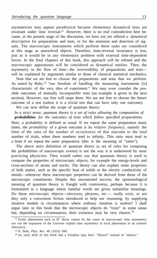
Introducing the quantum language 13
asymmetries may appear paradoxical because elementary dynamical laws areinvariant under time reversal.12 However, there is no real contradiction here be-cause, at the present stage of the discussion, we have not yet offered a dynamicaldescription for preparations and tests, or for the emission and detection of sig-nals. The macroscopic instruments which perform these tasks are consideredat this stage as unresolved objects. Therefore, time-reversal invariance is lost,just as it would be in any elementary problem with external time-dependentforces. In the final chapters of this book, this approach will be refined and themacroscopic apparatuses will be considered as dynamical entities. Then, theasymmetry in the flow of time—the irreversibility of preparations and tests—will be explained by arguments similar to those of classical statistical mechanics.
Note that we are free to choose the preparations and tests that we perform.As stated by Bohr,13 “our freedom of handling the measuring instruments [is]characteristic of the very idea of experiment.” We may even consider the pos-sible outcomes of mutually incompatible tests (an example is given in the nextsection). However, our free will stops there. We are not free to choose the futureoutcome of a test (unless it is a trivial test that can have only one outcome).
We can now define the scope of quantum theory:In a strict sense, quantum theory is a set of rules allowing the computation ofprobabilities for the outcomes of tests which follow specified preparations.
Here, a probability is defined as usual: If we repeat the same preparation manytimes, the probability of a given outcome is its relative frequency, namely thelimit of the ratio of the number of occurrences of that outcome to the totalnumber of trials, when these numbers tend to infinity. This ratio must tend toa limit if we repeat the same preparation (this is the meaning of “same”).
The above strict definition of quantum theory (a set of rules for computingthe probabilities of macroscopic events) is not the way it is understood by mostpracticing physicists. They would rather say that quantum theory is used tocompute the properties of microscopic objects, for example the energy-levels andcross-sections of atoms and nuclei. The theory can also explain some propertiesof bulk matter, such as the specific heat of solids or the electric conductivity ofmetals—whenever these macroscopic properties can be derived from those of themicroscopic constituents. Despite this uncontested success, the epistemologicalmeaning of quantum theory is fraught with controversy, perhaps because it isformulated in a language where familiar words are given unfamiliar meanings.Do these microscopic objects—electrons, photons, etc.— really exist, or arethey only a convenient fiction introduced to help our reasoning, by supplyingintuitive models in circumstances where ordinary intuition is useless? I shallargue later in this book that the microscopic objects do “exist” in some sensebut, depending on circumstances, their existence may be very elusive.14
12 Exotic phenomena such as K0 decay cannot be the cause of macroscopic time asymmetry;nor can the expansion of the Universe explain time asymmetry in local phenomena in an isolatedlaboratory.
13 N. Bohr, Phys. Rev. 48 (1935) 696.14 An early draft of this book had a Freudian typo here: “illusive” instead of “elusive.”

14 Introduction to Quantum Physics
1-5. What is a measurement?
Science is based on the observation of nature. Most scientists tend to believethat there exists an objective reality, which is partly unknown to us. We acquireknowledge about this reality by means of measurements: These are processesin which an apparatus interacts with the physical system under study, in sucha way that a property of that system affects a corresponding property of theapparatus. Since there must be an interaction between the apparatus and thesystem, measuring one property of a system necessarily causes a disturbance tosome of its other properties. This is true even in classical physics, as we shallsee in Sect. 12-2. However, classical physics assumes that the property which ismeasured objectively exists prior to the interaction of the measuring apparatuswith the observed system.
Quantum physics, on the other hand, is incompatible with the propositionthat measurements discover some unknown but preexisting reality. For example,consider the historic Stern-Gerlach experiment15 whose purpose was to deter-mine the magnetic moment of atoms, by measuring the deflection of a neutralatomic beam by an inhomogeneous magnetic field. Let us compute the trajec-tory of such an atom by classical mechanics, as Stern and Gerlach would havedone in 1922. (The reader who is not interested in the details of this calculationcan skip the next page.) The Hamiltonian of the atom is
H P2=
2m– µ · B , (1.4)
where m is the mass of the atom, p its momentum, and µ its intrinsic magnetic
Fig. 1.5. Idealized Stern-Gerlach experiment: silver atoms evaporate in anoven O, pass through a velocity selector S, an inhomogeneous magnet M,and strike a detector D. All the impacts are found in two narrow strips.
15 W. Gerlach and O. Stern Z. Phys. 8 (1922) 110; 9 (1922) 349.

What is a measurement? 15
moment. If the latter is due to some kind of internal rotational motion arounda symmetry axis, we have µ = g S , where S is the angular momentum aroundthe center of mass of the atom, and g is a constant—the gyromagnetic ratio—which depends on the mass and charge distribution around the rotation axis.The magnetic field B is a function of r , the position of the center of mass of theatom (the variation of B over the size of the atom is completely negligible).
The classical equations of motion are obtained from the Poisson brackets
= [r , H ] PB = P/ m ,
= [ p , H ]PB = ∇ ( µ · B ),
= [ µ, H ] PB= g ( µ × B ).
(1.5)
(1 .6)
(1.7)
The last equation follows from [Sx , Sy ]PB = S z and its cyclic permutations. Notethat the internal variables S have vanishing Poisson brackets with the center ofmass variables r and p.
Equation (1.7) implies that µ precesses around the direction of B . This di-rection cannot be constant in space, since this would violate Maxwell’s equation∇ · B = 0. One can however approximately solve (1.7) if , the mean value ofB in the magnet gap, is much larger than the variation of B in that gap andif, moreover, the duration of passage of the atom through the magnet is muchlonger than its precession time 2π/g B. If these conditions hold, the atom willprecess many times around the direction of , so that we can neglect, on atime average, the components of µ orthogonal to . Let us write = e 1 B,where e 1 is a unit vector and B is a constant. It then follows from (1.7) thatµ · e1 is a constant, and we can, on a time average, replace µ by µ1 e1 , where
µ1 := µ · 1e . (1.8)
(The symbol := means “is defined as”.) From Eq. (1.6) we obtain
ddt
(e 1 · p) = µ1 B' , (1.9)
where B' : =(e1 · ∇ ) ( e1 · B ) depends only on the construction of the magnet.The force (1.6) acts during a time L /v, where v is the longitudinal velocity
of the atoms, and L is the length of the magnet. The transverse momentumimparted to the atoms by this force is µ1 B'L/v, and their deflection angleis µ –11 B'L/2E, where E = mv2. All these terms, except µ2 1, are determinedby the macroscopic experimental setup (the oven, the velocity selector, themagnet, etc.) and are fixed for a given experiment. The surprising result foundby Gerlach and Stern15 was that µ 1 could take only two values, ± µ.
This result is extremely surprising from the point of view of classical physics,because Gerlach and Stern could have chosen different orientations for theirmagnet, for example e 2 and e 3 , making angles of ±120° with e 1 , as shown inFig. 1.6. They would have measured then

16 Introduction to Quantum Physics
µ2 = µ · e2 or µ3 = µ · e3 , (1.10)
respectively. As the laws of physics cannot be affected by merely rotating themagnet, they would have found, likewise,µ2 = ± µ or µ3 = ± µ. This creates,however, an apparent contradiction when we add Eqs. (1.8) and (1.10):
µ1 + µ2 + µ3 = µ · (e1 + e 2 + e3) ≡ 0. (1.11)
Obviously, µ1 , µ2 and µ3 cannot all be equal to ±µ , and also sum up to zero.Of course, it is impossible to measure in this way the values ofµ1 and µ2
a n dµ3 of the same atom—the magnet can have only one of the three positions.There is no need to invoke “quantum uncertainties” here. This is a purelyclassical impossibility, inherent in the experiment described by Fig. 1.6. (What
Fig. 1.6. Three possible orientations for the Stern-Gerlach magnet, making 120°angles with each other. The three unit vectors e1 , e 2 and e 3 sum up to zero.
quantum theory tells us is that this is not a defect of this particular experimentalmethod for measuring a magnetic moment: No experiment whatsoever candetermineµ1 and µ2 and µ3 simultaneously.) Yet, even if the three experimentalsetups sketched in Fig. 1.6 are incompatible, it is certainly possible16 to measureµ2 , or µ3, instead ofµ1. Thus, if we attribute to the word “measurement” itsordinary meaning, namely the acquisition of knowledge about some objectivepreexisting reality, we reach a contradiction.
The contradiction is fundamental. Once we associate discrete valueswith the components of a vector which can be continuously rotated,the meaning of these discrete values cannot be that of “objective” vectorcomponents, which would be independent of the measurement process.
16You may feel uneasy with this counterfactual reasoning. While we are free to imagine thepossible outcomes of unperformed experiments, Eq. (1.11) goes farther: it involves, simultane-ously, the results of three incompatible experiments. At most one of the mathematical symbolswritten on the paper can acquire an actual meaning. The two others then exist only in ourimagination. Is that equation legitimate? Can we draw from it reliable conclusions? Moreover,Eq. (1.11) assumes that, in these three possible but incompatible experiments, the magneticmoment of the silver atom has the same orientation. That is, our freedom of choice for theorientation of the magnet does not affect the silver atoms that evaporate from the oven. If youthink that this is obvious, wait until after you have read Chapter 6.

What is a measurement? 17
A measurement is not a passive acquisition of knowledge. It is an active pro-cess, making use of extremely complex equipment, usually involving irreversibleamplification mechanisms. (Irreversibility is not accidental, but essential, if wewant an objective, indelible record. The record must be objective, even if the“physical quantity” to which it refers is not. This point will be discussed inChapter 12). Moreover, we must interpret the experimental outcomes producedby our equipment. We do that by constructing a theoretical model whereby thebehavior of the macroscopic equipment is described by a few degrees of freedom,interacting with those of the microscopic system under observation. We thencall this a “measurement” of the microscopic system. The logical conclusionfrom this procedure was drawn long ago by Kemble:17
We have no satisfactory reason for ascribing objective existence to physicalquantities as distinguished from the numbers obtained when we make themeasurements which we correlate with them. There is no real reason forsupposing that a particle has at every moment a definite, but unknown,position which may be revealed by a measurement of the right kind, ora definite momentum which can be revealed by a different measurement.On the contrary, we get into a maze of contradictions as soon as we injectinto quantum mechanics such concepts carried over from the languageand philosophy of our ancestors... It would be more exact if we spoke of“making measurements” of this, that, or the other type instead of sayingthat we measure this, that, or the other “physical quantity.”
As a concrete example, consider again the Stern-Gerlach experiment sketchedin Fig. 1.5. The theoretical model corresponding to it is given by Eq. (1.4). Themicroscopic object under investigation is the magnetic moment µ of an atom—more exactly, itsµ1 component. The macroscopic degree of freedom to which itis coupled in this model is the center of mass position r (the coupling is in theterm µ·B, since B is a function of r). I call this degree of freedom macroscopicbecause different final values of r can be directly distinguished by macroscopicmeans, such as the detectors sketched in Fig. 1.5 (see Exercise 1.8). Fromhere on, the situation is simple and unambiguous, because we have entered themacroscopic world: The type of detectors and the details of their functioningare deemed irrelevant. No additional theoretical model is needed to interpretthe conspicuously macroscopic event which occurs when a particular detectoris excited. The use of these detectors is only a convenient amplification of anexisting signal, for the benefit of the experimenter.
Nevertheless, if we have doubts about this interpretation, we can displacethe arbitrary boundary between the microscopic and the macroscopic worlds.We have the right to consider the numerous atoms in the detectors as addi-tional parts of the observed system, to include all their degrees of freedom inthe Hamiltonian (with all the interactions between these atoms and those of
17E. C. Kemble, The Fundamental Principles of Quantum Mechanics, McGraw-Hill, NewYork (1937) [reprinted by Dover] pp. 243-244.

18 Introduction to Quantum Physics
the atomic beam) and to imagine an additional, larger apparatus observing thewhole thing. Consistency requires that the result of observing the detectors byanother instrument is the same as if the detectors themselves are considered asthe ultimate instrument. This is what is meant by the claim that there is anobjective record of the experiment. The role of physics is to study relationshipsbetween these objective records. Some people prefer to use the word “inter-subjectivity,” which means that all observers agree about the outcome of anyparticular experiment. Whether or not there exists an objective “reality” be-yond the intersubjective reality may be an interesting philosophical problem,18
but this is not the business of quantum theory. As explained at the end ofSect. 1-4, quantum theory, in a strict sense, is nothing more than a set of ruleswhereby physicists compute probabilities for the outcomes of macroscopic tests.
Exercise 1.8 Show that, in the Stern-Gerlach experiment, the quantum me-chanical spreading of the wave packet of a free silver atom is negligible. There-fore the motion of its center of mass can safely be treated by classical mechanics,once the magnetic moment of the atom does not interact with external fields.Hint: What is the diffraction angle of a beam with λ = h/p and aperturedetermined by the collimators in the Stern-Gerlach experiment?
Exercise 1.9 Rewrite the Stern-Gerlach calculation in quantum notations,with commutators instead of Poisson brackets, and with S represented by 2 × 2matrices. Is Eq. (1.11) still valid? Where will the classical argument which ledto a contradiction break down?
Exercise 1.10 What are the possible values of Sx , S and S for a particle ofy zspin S = –3? Can you combine these values so that S2 + S2 + S 2 = S ( S + 1)?2 x y z
1-6. Historical remarks
The interference properties of polarized light were discovered in the early 19thcentury by Arago and Fresnel.19 Decades before Maxwell, the phenomenologysketched in Fig. 1.4 was known. The crisis of classical determinism could there-fore have erupted already in 1905, as soon as it became apparent from the workof Planck¹ and Einstein² that light consisted of discrete, indivisible entities.But at that time, no one was worried by such difficulties, because too manyother facts were unexplained. Nobody knew how to compute the frequenciesof spectral lines, nor their intensities. In fact, nobody understood why atomswere stable and could exist at all.
Progress was slow. First, came the “old” quantum theory. In 1913, Bohr20
suggested that the only stable electronic orbits were those for which the angular
18B. d’Espagnat, Une incertaine réalité, Bordas, Paris (1985); English transl.: Reality andthe Physicist, Cambridge Univ. Press (1989).
19F. Arago and A. Fresnel, Ann. de Chimie et Physique 10 (1819) 288.20N. Bohr, Phil. Mag. 26 (1913) 1, 476, 857.

Historical remarks
Par MM. ARAGO et FRESNEL.
Sur l’ Action que les rayons de lumiére polarisésexercent les uns sur les autres.
AVANT de rapporter les expériences qui font l’objet dece Mémoire, il ne sera peut-être pas inutile de rappelerquelques-uns des beaux résultats que le Dr ThomasYoung avait déjà obtenus en étudiant, avec cette raro
sagacité qui le caractérise, l’influence que, dans cer-taines circonstances, les rayons de lumière exercent lesuns sur les autres.
1°. Deux rayons de lumière homogène, émanant d’uneméme source, qui parviennent en un certain point
de l’espace par deux routes différentes et légèrement
inégales, s’ajoutent ou se détruisent, forment sur l'écran
qui les reçoit un point clair ou obscur, suivant que ladifférence des routes a telle ou telle autre valeur.
2°. Denx rayons s’ajoutent constamment là où ils ont
parcouru des chemins égaux: si l’on trouve qu’ils s’a-
joutent de nouveau quand la différence des deux chemins
M É M O I R E
19
Fig. 1.7. The historic paper of Arago and Fresnel19 on the interference ofpolarized light starts by recalling “some of the beautiful results alreadyobtained by Dr. Thomas Young on the interference of light rays.”
momentum was an integral multiple of h /2π. Planck’s constant h, originallyintroduced to explain the properties of thermal radiation, was found relevant tothe mechanical properties of atoms too. Unfortunately, Bohr’s ad hoc hypoth-esis, which correctly gave the energy levels of the hydrogen atom—the simplestatom—already failed for the next simplest one, helium.
Exercise 1.11 Bohr’s model for the helium atom consists of two electronsrevolving at diametrically opposed points of a circular orbit, around a point-likenucleus at rest. Find the lowest energy level from the condition that the angularmomentum of each electron is . Compare your result with the experimentalionization energy of helium.
Bohr’s hypothesis was generalized by Wilson21 and Sommerfeld22 to dynami-cal systems with several separable degrees of freedom, and then by Einstein23 to
21W. Wilson, Phil. Mag. 29 (1915) 795.22A. Sommerfeld, Ann. Physik 51 (1916) 1.23A. Einstein, Verh. Deut. Phys. Gesell. 19 (1917) 82.

20 Introduction to Quantum Physics
systems which were not separable, but still were integrable. However, more gen-eral aperiodic phenomena, such as the scattering of atoms or their interactionin the formation of molecules, remained practically untouched.
The next progress was due to de Broglie.24 His doctoral thesis, submittedin 1924, was effectively the counterpart of the hypothesis that Einstein hadproposed in 1905 to explain the photoelectric effect. Not only were electro-magnetic waves endowed with particle-like properties, but material particlessuch as electrons could display wave-like behavior. The relationship p = h / λwas universal, and Bohr’s angular momentum postulate simply meant that thelength of an electronic orbit was an integral number of electronic wavelengths.This unified view of nature was aesthetically appealing, but it could not yet beconsidered as a consistent theory.
The following year, Heisenberg25 invented a “matrix mechanics” in whichenergy levels were the eigenvalues of infinite matrices. Lanczos26 showed thatHeisenberg’s infinite matrices could be represented as singular kernels in inte-grals and was able to derive an integral equation whose eigenvalues were the in-verse energy levels. However, Lanczos’s work attracted little attention becauseit was soon superseded by Schrödinger’s “wave mechanics” in which energy lev-els were the eigenvalues of a differential operator (which is notoriously easierto use than an integral operator). Schrödinger, who was led to his theory bya study of de Broglie’s work, also proved the mathematical equivalence of hisapproach and that of Heisenberg.27
The “new” quantum theory became known as quantum mechanics and devel-oped very rapidly. There were important contributions by Born and Jordan28
and especially by Dirac,29 who successfully guessed a relativistic wave equationfor the electron. Quantum mechanics was unambiguous and mathematicallyconsistent. It allowed to compute not only the properties of the hydrogenatom, but also those of the helium atom—in principle those of any atom, anymolecule, anything for which the potential was known. It would correctly pre-dict the probabilities for photons to go one way or the other in a calcite crystalbut, on the other hand, it could not predict the path taken by a particularphoton. Therefore that theory was essentially statistical.
Not everyone was happy with this novel feature, in particular Einstein wasnot. He clearly understood that the meaning of quantum mechanics could onlybe statistical. He wrote, near the end of his life:30
One arrives at very implausible theoretical conceptions, if one attemptsto maintain the thesis that the statistical quantum theory is in principle
24L. de Broglie, Ann. Physique (10) 3 (1925) 22.25W. Heisenberg, Z. Phys. 33 (1925) 879.26K. Lanczos, Z. Phys. 35 (1926) 812.27E. Schrödinger, Ann. Physik 79 (1926) 361, 489, 734.28M. Born and P. Jordan, Z. Phys. 34 (1925) 858.29P. A. M. Dirac, Proc. Roy. Soc. A 117 (1928) 610.30A. Einstein, in Albert Einstein, Philosopher-Scientist, ed. by P. A. Schilpp, Library of
Living Philosophers, Evanston (1949), pp. 671-672.

Bibliography 21
capable of producing a complete description of an individual physical
system. . .I am convinced that everyone who will take the trouble to carrythrough such reflections conscientiously will find himself finally driven tothis interpretation of quantum-theoretical description (the ψ-function isto be understood as the description not of a single system but of an en-semble of systems). . . There exists, however, a simple psychological reasonfor the fact that this most nearly obvious interpretation is being shunned.For if the statistical quantum theory does not pretend to describe theindividual system (and its development in time) completely, it appearsunavoidable to look elsewhere for a complete description of the individualsystem. . . Assuming the success of efforts to accomplish a complete physicaldescription, the statistical quantum theory would, within the framework offuture physics, take an approximately analogous position to the statisticalmechanics within the framework of classical mechanics. I am rather firmlyconvinced that the development of theoretical physics will be of that type;but the path will be lengthy and difficult.
Since the inception of quantum mechanics, many theorists have labored toprove, or disprove, the possible existence of theories with “hidden variables”whereby the quantum wave function would be supplemented by additional datain order to restore a neoclassical determinism. The unexpected result of theseinvestigations were proofs by Bell,31 and by Kochen and Specker,32 that hiddenvariables could actually be introduced in such a way that statistical averagesover their values reproduced the results of quantum mechanics. There washowever a heavy price to pay for this reinstatement of determinism: the hiddenvariables of two widely separated and noninteracting systems were, in somecases, inseparably entangled. Therefore determinism could be restored only atthe cost of abandoning the axiom of separability—the mutual independence ofvery distant systems—which until that time had been considered as obvious.This quantum inseparability will be discussed in Chapter 6. Its philosophicalimplications are profound. They have been the subject of a lively debate whichwill probably continue for many years to come.
1-7. Bibliography
The reader of this book is assumed to be reasonably familiar with classicalphysics. To remedy possible deficiencies, the following textbooks are suggested:
Thermal radiation
L. D. Landau and E. M. Lifshitz, Statistical Physics, 2nd ed., Pergamon,Oxford (1969) Chapt. 5.
31J. S. Bell, Physics 1 (1964) 195; Rev. Mod. Phys. 38 (1966) 447.32S. Kochen and E. P. Specker, J. Math. Mech. 17 (1967) 59.
22 Introduction to Quantum Physics
F. K. Richtmyer, E. H. Kennard, and J. N. Cooper, Introduction to ModernPhysics, 6th ed., McGraw-Hill, New York (1969) Chapt. 5.
Crystal optics
M. Born and E. Wolf, Principles of Optics, 6th ed., Pergamon, Oxford (1980)Chapt. 14.
S. G. Lipson and H. Lipson, Optical Physics, 2nd ed., Cambridge U. Press(1981) Chapt. 5.
Poisson brackets
H. Goldstein, Classical Mechanics, 2nd ed., Addison-Wesley, Reading (1980)Chapt. 9.
L. D. Landau and E. M. Lifshitz, Mechanics, 3rd ed., Pergamon, Oxford(1976) Chapt. 7.
“Old” and “new” quantum theory
M. Born, The mechanics of the atom, Bell, London (1927) [reprinted byUngar, New York (1960)].
This remarkable book was originally published in 1924 under the title “Atom-mechanik.” In the preface to the English translation, completed in January 1927,the author wrote:
Since the appearance of this book in German, the mechanics of the atomhas developed with a vehemence that could scarcely be foreseen. The newtype of theory which I was looking for as the subject matter of the projectedsecond volume has already appeared in the new quantum mechanics, whichhas been developed from two quite different points of view. I refer on theone hand to the quantum mechanics which was initiated by Heisenberg,and developed by him in collaboration with Jordan and myself in Germany,and by Dirac in England, and on the other hand to the wave mechanicssuggested by de Broglie, and brilliantly worked out by Schrödinger. Theseare not two different theories, but simply two different modes of exposition.Many of the theoretical difficulties discussed in this book are solved by thenew theory.
Born’s book is one of the best sources on canonical transformations, action-anglevariables and the Hamilton-Jacobi theory. These were the indispensable tools of the-orists who practiced the old quantum theory. Curiously, the book does not mentionPoisson brackets. The latter became of special interest only at a later stage, with theadvent of Heisenberg’s and Dirac’s formulations of the “new” quantum theory.
Another classic reference for the “old” quantum theory is
A. Sommerfeld, Atomic Structure and Spectral Lines, Methuen, London(1923).
This is a translation of the third edition of Atombau und Spektrallinien, Vieweg,Braunschweig (1922). The fourth German edition (1924) was not translated.

Bibliography 23
B. L. van der Waerden, editor, Sources of Quantum Mechanics, North-Holland, Amsterdam (1967) [reprinted by Dover].
This book contains the English text (original or translated) of 17 historic articles onquantum theory, starting with Einstein’s “Quantum Theory of Radiation” (1917), andending with the works of Heisenberg, Born, Jordan, Dirac, and Pauli. It is remarkablethat Schrödinger’s work is totally ignored. The inventors of quantum mechanics—in itsoriginal matrix form—were dismayed by the success of Schrödinger’s “wave mechanics,”which promptly superseded matrix mechanics in nearly all applications.
Recommended reading
J. B. Hartle, “Quantum mechanics of individual systems,” Am. J. Phys. 36(1968) 704.
This is a lucid explanation that a quantum “state is not an objective property of anindividual system, but is that information, obtained from a knowledge of how the systemwas prepared, which can be used for making predictions about future measurements . . .The ‘reduction of the wave packet’ does take place in the consciousness of the observer,not because of any unique physical process which takes place there, but only becausethe state is a construct of the observer and not an objective property of the physicalsystem.”
D. Finkelstein, “The physics of logic,” in Paradigms and Paradoxes, editedby R. C. Colodry, Univ. Pittsburgh Press (1971), Vol. V; reprinted in Logico-Algebraic Approach to Quantum Mechanics, edited by C. A. Hooker, Reidel,Dordrecht (1975), Vol. II, pp. 141–160.
J. M. Jauch, Are Quanta Real? A Galilean Dialogue, Indiana Univ. Press,Bloomington (1973).
L. E. Ballentine, “The statistical interpretation of quantum mechanics,”Rev. Mod. Phys. 42 (1970) 358.
H. P. Stapp, “The Copenhagen interpretation,” Am. J. Phys. 40 (1972) 1098.
The experts disagree on what is meant by “Copenhagen interpretation.” Ballentinegives this name to the claim that “a pure state provides a complete and exhaustivedescription of a single system.” The latter approach is called by Stapp the “absolute-ψinterpretation.” Stapp insists that “critics often confuse the Copenhagen interpretation,which is basically pragmatic, with the diametrically opposed absolute-ψ interpretation. . . In the Copenhagen interpretation, the notion of absolute wave function representing
the world itself is unequivocally rejected.” There is therefore no real conflict betweenBallentine and Stapp, except that one of them calls Copenhagen interpretation whatthe other considers as the exact opposite of the Copenhagen interpretation.
Chapter 2
QuantumTests
2-1. What is a quantum system?
A quantum system is a useful abstraction, which frequently appears in theliterature, but does not really exist in nature. In general, a quantum system isdefined by an equivalence class of preparations. (Recall that “preparations” and“tests” are the primitive notions of quantum theory. Their meaning is the set ofinstructions to be followed by an experimenter.) For example, there are manyequivalent macroscopic procedures for producing what we call a photon, or afree hydrogen atom, etc. The equivalence of different preparation proceduresshould be verifiable by suitable tests.
The ambiguity of these notions emerges as soon as we think of concreteexamples. Is a hydrogen atom in a 2p state the same system as one in a 1sstate? Or is it the same system as a hydrogen atom in a 1s state accompaniedby a photon? The answer depends on the problem in which we are interested:energy levels or transition rates. In a Stern-Gerlach experiment, we have seen(page 17) that the “quantum system” is not a complete silver atom. It is onlythe magnetic momentµ of that atom, because the goal of the Stern-Gerlachtest is to determine a component ofµ. The center of mass of the atom canbe treated classically. These examples show that we must be content with avague “definition”: A quantum system is whatever admits a closed dynamicaldescription within quantum theory.
While quantum systems are somewhat elusive, quantum states can be givena clear operational definition, based on the notion of test. Consider a givenpreparation and a set of tests, among which some are mutually incompatible, asin Fig. 1.6. If these tests are performed many times, after identical preparations,we find that the statistical distribution of outcomes of each test tends to a limit.Each outcome has a definite probability. We can then define a state as follows:A state is characterized by the probabilities of the various outcomes of everyconceivable test.
This definition is highly redundant. We shall soon see that these probabilitiesare not independent. One can specify—in many different ways—a restricted set
24

What is a quantum system? 25
of tests such that, if the probabilities of the outcomes of these tests are known,it is possible to predict the probabilities of the outcomes of every other test.(A geometric analogy is the definition of a vector by its projections on everyaxis. These projections are not independent: it is sufficient to specify a finitenumber of them, on a complete, linearly independent set of axes.)
Before we examine concrete examples, the notion of probability should beclarified. It means the following. We imagine that the test is performed aninfinite number of times, on an infinite number of replicas of our quantumsystem, all identically prepared. This infinite set of experiments is called astatistical ensemble. It should be clearly understood that a statistical ensembleis a conceptual notion—it exists only in our imagination, and its use is tohelp our reasoning.1 In this statistical ensemble, the occurrence of event A hasrelative frequency P A; it is this relative frequency which is called a probability.To actually measure a probability, the best we can do is to repeat the sameexperiment a large (but finite) number of times.1 The more we repeat it, thesmaller will be the expected difference between the measured relative frequencyand the true probability.
As a simple example of definition of a state, suppose that a photon is saidto have right-handed polarization. Operationally, this means that if we sub-ject that photon to a specific test (namely, a quarter wave plate followed by asuitably oriented calcite crystal) we can predict with certainty that the photonwill exit in a particular channel. For any other test, consisting of arbitrarilyarranged calcite crystals and miscellaneous optically active media, we can thenpredict probabilities for the various exit channels. (These probabilities are com-puted in the same way as the classical beam intensities.) Note that the word“state” does not refer to the photon by itself, but to an entire experimentalsetup involving macroscopic instruments. This point was emphasized by Bohr:2
There can be no unambiguous interpretation of the quantum mechanicssymbols other than that embodied in the well-known rules which allow topredict the results to be obtained by a given experimental arrangementdescribed in a totally classical way.
More generally, we may relate a quantum state to a set of equivalent experi-mental procedures—provided that it is in principle possible to verify that theseprocedures are indeed equivalent. For instance, we may use quarter wave platessupplied by different manufacturers, or we may devise an altogether differentmethod to analyze circular polarization. Occasionally, we may even renouncethe use of any equipment, and consider purely mental experiments, as long aswe are sure that a real experiment is possible in principle. For example, it isperfectly legitimate to consider the state of an electron located at the center ofthe Sun. A measurement of a spin component of that electron is undoubtedly
1 Repeating an experiment a million times does not produce an ensemble. It only makes onevery complex experiment, involving a million approximately similar elements. (In this book,the term assembly is used to denote a set of almost identical systems.)
2 N. Bohr, Phys. Rev. 48 (1935) 696.

26 Quantum Tests
very difficult, and it is ruled out for sure by budgetary constraints; but it isnot ruled out by the laws of physics—as they are known today. Therefore itis legitimate to use quantum mechanics to compute the physical properties ofa stellar plasma, just as it is used to discuss metallic conduction, or heliumsuperfluidity, that we observe in our laboratory.
The essence of quantum theory is to provide a mathematical representationof states (that is, of preparation procedures), together with rules for computingthe probabilities of the various outcomes of any test. Our first task thus is to getacquainted with the phenomenology of quantum tests. I shall start by listingsome basic empirical facts. The conceptual implications of these facts will beanalyzed, and then elevated to the status of “postulates.” However, it will not bepossible to derive the complete formal structure of quantum theory from theseempirically based postulates. Additional postulates will have to be introduced,with mathematical intuition as our only guide; and the consequences derivedfrom these new postulates will have to be tested experimentally.
Before we enter into these details, the nature of a quantum test must beclearly understood. A test is more than the mere occurrence of an unpredictableevent, such as the blackening of a grain in a photographic plate, or an electricdischarge in a particle detector. To be interesting to physicists, these macro-scopic events must be accompanied by a theoretical interpretation. As explainedabove, the latter must be partly classical.
For example, the firing of one of the photodetectors in Fig. 1.3 is interpretedas the arrival of a polarized photon, because we tacitly use the rules of classicalelectromagnetic theory, according to which a beam of light is split by a calcitecrystal into two beams with opposite polarizations. Likewise, the Stern-Gerlachexperiment is interpreted as the measurement of a magnetic moment, becauseit could indeed be such a measurement if we just sent little compass needlesthrough the Stern-Gerlach magnet, instead of sending silver atoms. When nu-clear physicists measure cross sections, they assume that the nuclear fragmenttrajectories are classical straight lines between the target and the various detec-tors. Without this assumption, the macroscopic positions of the detectors couldnot be converted into angles for the differential nuclear cross sections. And whenspectroscopists measure wavelengths by means of diffraction gratings, they useclassical diffraction theory to convert their data into wavelengths. Quantumtheory appears only at the next stage, to explain, or predict, the possible valuesof the magnetic moment, the cross sections, the wavelengths, etc.
Here, you may ask: Why can’t we describe the measuring instrument byquantum theory too? We can, and we shall indeed do that later, in order toprove the internal consistency of the theory. However, this only shifts the imagi-nary boundary between the quantum world—which is an abstract concept—andthe mundane, tangible world of everyday. If we quantize the original classicalinstrument, we need another classical instrument to measure the first one, andto record the permanent data that will remain available to us for further study.
This mental process can be repeated indefinitely. Some authors state thatthe last stage in this chain of measurements involves “consciousness,” or the

Repeatable tests 27
“intellectual inner life” of the observer, by virtue of the "principle of psycho-physical parallelism.” 3,4 Other authors introduce a wave function for the wholeUniverse.5 In this book, I shall refrain from using concepts that I do not un-derstand. The internal consistency of the theory will simply mean that if aninstrument is quantized and observed by another instrument, whose descriptionremains classical, the result obtained by the second instrument must agree withthe result that was registered by the first one, when the first one was describedclassically. More precisely, the probability for obtaining conflicting results mustbe arbitrarily low. This requirement imposes conditions on what can legiti-mately be called a measuring apparatus. It will be shown that an apparatusmust have enough degrees of freedom to behave irreversibly in a thermodynamicsense. This will establish the consistency of our approach.
2-2. Repeatable tests
Consider two consecutive identical tests, following each other with a negligibletime interval between them. If these tests always yield identical outcomes,they are called repeatable. (The term “repeatable” is used to refer to testswhose outcomes are intrinsically unpredictable, except statistically, for mostpreparations that may precede these tests. The term “reproducible” refers tophenomena having a fully predictable behavior.)
For example, consider two identical calcite crystals, arranged for testing thelinear polarizations of incoming photons, as in Fig. 2.1. There are three de-tectors. It is found empirically that only the upper and lower ones may beexcited; the central one never is. This is indeed what classical electromagnetictheory predicts for light rays: any trajectory different from those indicated bythe dotted lines is impossible to achieve. Note that we must tacitly imagine theexistence of quasi-classical paths, as indicated by the dotted lines, because thisis the only way of interpreting the outcome of the experiment. Without somekind of interpretation, experiments are meaningless.
There is, however, a delicate point here: We also tacitly assume that theroute followed by a photon, when it is tested by the first calcite crystal, does notdepend on the existence of the second calcite crystal that we placed between thefirst one and the detectors. We believe that this photon would have followed thesame route even if the second crystal had not been present. Such an assumptionis needed in order to be able to say that there are two consecutive tests here,and to compare their results, in spite of the fact that the result of the first testis not recorded, but only inferred. This assumption is natural, because of our
3J. von Neumann, Mathematische Grundlagen der Quantenmechanik, Springer, Berlin(1932) p. 223; transl. by E. T. Beyer: Mathematical Foundations of Quantum Mechanics,Princeton Univ. Press, Princeton (1955) p. 418.
4 E. P. Wigner, Symmetries and Reflections, Indiana Univ. Press, Bloomington (1967) p. 177.5 J. B. Hartle and S. W. Hawking, Phys. Rev. D 28 (1983) 2960.

28 Quantum Tests
deeply rooted classical prejudices—we have a tendency to imagine that eachphoton follows a well defined trajectory. However, this assumption is obviouslycounterfactual, and it is not verifiable. Counterfactual experiments will furtherbe discussed in Chapter 6, where it will be seen that our intuition is not at alla reliable guide in the quantum domain.
Fig. 2.1. A repeatable test: the second calcite crystalalways confirms the result given by the first one.
Not every test is repeatable. For example, if identical quarter wave plateswere affixed to the right of each calcite crystal in Fig. 2.1, there would be threeoutgoing rays, rather than two, emerging from the second crystal (the centraldetector would be excited as frequently as the two others combined). In thatcase, the photons leaving the first test would be circularly polarized. This isnot the kind of polarization that is tested by these calcite crystals—thereforethe modified tests would not be repeatable.
These tests would also not be repeatable if an optically active fluid wereintroduced between the two crystals, causing a rotation of the polarizationplane. Likewise, two consecutive identical Stern-Gerlach experiments, with theirmagnetic fields parallel, may yield conflicting results if they are separated by aregion where a perpendicular magnetic field causes a precession of the magneticmoment of the atom. The dynamical evolution of quantum systems will bediscussed in Chapter 8. In the present chapter, it is assumed that consecutivetests follow each other so rapidly that we can neglect any dynamical evolutionbetween them.
Another example of nonrepeatable test is the standard method for measuringthe momentum of a neutron, by observing the recoil of a proton in a photo-graphic emulsion or in a bubble chamber. It is obvious that the momentumof the neutron after the measurement cannot be the same as before it. Thisexample clearly shows that a good measurement is not necessarily repeatable,contrary to careless statements such as6
From physical continuity, if we make a second measurement of the samedynamical variable immediately after the first, the result of the secondmeasurement must be the same as that of the first.
6 P. A. M. Dirac, The Principles of Quantum Mechanics, Oxford Univ. Press (1947), p. 36.

Maximal quantum tests 29
This gives the impression that every correctly done test is necessarily repeatable.Actually, repeatable tests are the exception, not the rule. They exist mostly inthe imagination of theorists. They are idealizations, like rigid bodies, or Carnotengines; and like them, they are useful in theoretical discussions. The reasonwill soon be obvious, when we consider consecutive tests that differ from eachother (see Sect. 2-4).
In most of this book, I shall therefore assume that tests have been designedso as to be repeatable, and the word “test” will mean a repeatable test, unlessspecified otherwise. However, it must be emphasized that nonrepeatable testsare the most common variety. Moreover, they may yield more information thanideal repeatable tests, as you will see in Chapter 9.
2-3. Maximal quantum tests
Let N be the maximum number of different outcomes obtainable in a test ofa given quantum system. Assume N to be finite, for simplicity (the case ofinfinite N will be discussed in Chapter 4). Then, any test that has exactlyN different outcomes is called maximal or complete. For example, the Stern-Gerlach experiment sketched in Fig. 1.5 is a complete test for the value of acomponent of a magnetic moment. It always has, irrespective of the orientationof the magnet, (2s + 1) different outcomes for atoms of spin s. An incompletetest is one where some outcomes are lumped together, for example, becausethe experimental equipment has insufficient resolution. This is not necessarilya defect. We shall see (Chapter 12) that a low resolution may be advantageousin some applications, and that “fuzzy measurements” sometimes are those fromwhich we can extract the most interesting information. They should not beconfused with imperfect tests, whose outcomes are afflicted by various detectorinefficiencies (including false alarms).
The adjective maximal or complete should not be misunderstood. A linearpolarization test, such as the one sketched in Fig. 1.3, is complete only withrespect to the polarization of the photon. It yields no information about otherproperties that the photon may have, such as its position or momentum. Like-wise, the Stern-Gerlach experiment (Fig. 1.5) is a complete test for spin, whileother degrees of freedom are ignored. In practice, the result of each one of thesetests is observed by correlating the value of the internal degree of freedom (po-larization or spin) which is being tested, to the position of the outgoing particle,which can then be detected by macroscopic means.
The notion of completeness of a quantum test is radically different fromits counterpart in classical physics. For example, in classical mechanics, itis possible to specify all the components of the angular momentum J of arotating body. A complete description of the body must therefore include allof them. However, when we attempt to measure the components of J of verysmall systems such as atoms, we find empirically that the measurement of

30 Quantum Tests
one of the components of J not only precludes the measurement of the othercomponents, but it even alters the expected values of these other componentsin an uncontrollable way. An example was given in Sect. 1-5 when we discussedthe Stern-Gerlach experiment. It was shown that the atom had to precess manytimes around the direction of —the mean value of the magnetic field—so thatthe components of J perpendicular to were randomized. This result mayappear at first as an irrelevant practical difficulty, due to the limitations ofthe experimental setup chosen by Gerlach and Stern. However, this difficultybecomes a matter of principle in quantum theory. To be precise, if we choose touse quantum theory as the tool for interpreting the results of our experiments,it is impossible to exactly determine more than one component of the angularmomentum.7 We can only choose the component which we want to determine.
This limitation does not preclude the use of quantum mechanics for comput-ing the motion of a gyroscope, say, if we wish to do so. We shall see that, inthe semiclassical limit J » , it is in principle possible to reduce the uncer-tainty in each one of the components of J to a value of the order of Thisuncertainty is utterly negligible for macroscopic systems, such as gyroscopes.Quantum limitations, as mentioned above, arise only when we want to reducethe uncertainty in one of the components of J to less than
It should be clear that the interpretation of raw experimental data alwaysnecessitates the use of some theory. Concepts such as “angular momentum” areparts of the theory, not of the experiment. Moreover, correspondence rules areneeded to relate the abstract notions of the theory to our laboratory hardware.It is the theory—together with its correspondence rules—which tells us whatcan, or cannot, be measured. What does not exist in the theory cannot beobserved in any experiment to be described by that theory. Conversely, anythingdescribed by the theory is deemed to be observable, unless the theory itselfprohibits to observe it. To be acceptable, a theory must have predictive powerabout the outcomes of the experiments that it describes, so that the theory caneventually fail. A “good” theory is one which does not fail in its domain ofapplicability. Today, in our present state of knowledge, quantum theory is thebest available one for describing atomic, nuclear, and many other phenomena.
According to quantum theory, we have a choice between different, mutuallyincompatible tests. For example, we may orient the Stern-Gerlach magnet inany direction we please. Why then is such a Stern-Gerlach test called complete?The reason can be stated as the following postulate:
A. Statistical determinism. If a quantum system is preparedin such a way that it certainly yields a predictable outcome in aspecified maximal test, the various outcomes of any other test havedefinite probabilities. In particular, these probabilities do not de-pend on the details of the procedure used for preparing the quantumsystem, so that it yields a specific outcome in the given maximal test.A system prepared in such a way is said to be in a pure state.
7 There is one exception: all the components of J may vanish simultaneously.
Maximal quantum tests 31
The simplest method for producing quantum systems in a given pure state isto subject them to a complete test, and to discard all the systems that didnot yield the desired outcome. For example, perfect absorbers may be insertedin the path of the outgoing beams that we do not want. When this has beendone, all the past history of the selected quantum systems becomes irrelevant.The fact that a quantum system produces a definite outcome, if subjected to aspecific maximal test, completely identifies the state of that system, and this isthe most complete description that can be given of it.8
The next definition we need is that of equivalent tests:
B. Equivalence of maximal tests . Two maximal tests areequivalent if every preparation that yields a definite outcome forone of these tests also yields a definite outcome for the othertest. In that case, any other preparation (namely one that doesnot yield a predictable outcome for these tests) will still yield thesame probabilities for corresponding outcomes of both tests.
For example, a Stern-Gerlach experiment measuring Jz (for arbitrary spin) isequivalent to an experiment measuring (Jz )3 , or 1/(J z – , or any othersingle valued function of Jz . It is important to note that postulate B demandsthat N different preparations yield definite and different outcomes for eachone of the maximal tests. Equivalence is not guaranteed for tests that merelyyield, in some cases, identical probabilities. For example, consider two crystalswhich can test linear polarization. Each one of these crystals, regardless of itsorientation, will split an incoming beam of circularly polarized light into twobeams of equal intensities, so that both tests always agree, statistically, in thespecial case of circularly polarized light (for both circular polarizations!). Thistrivial result gives of course no information as to what would happen if a beamof linearly polarized light impinged on one of these crystals, and in particularwhether that beam would be split in the same proportions by both crystals.
In real life, most preparations do not yield pure states, but mixed ones. Afteran imperfect preparation, no maximal test has a predictable outcome. Forexample, photons originating from an incandescent lamp are in a mixed stateof polarization. In this particular case, their polarization is completely random.Any test for polarization (whether linear, circular or, in general, elliptic) shouldyield approximately equal numbers of photons with opposite polarizations, ifthe apparatus has the same efficiency for both outcomes of that test. Such anapparatus is called unbiased, and we shall henceforth consider only unbiasedtests. This example suggests the following generalization:
C. Random mixtures. Quantum systems with N states can beprepared in such a way that every unbiased maximal test has thesame probability, N –1 , for each one of its outcomes.
8Any attemp t to supplement this description by means of additional “hidden” variables leadsto serious difficulties. See discussion in Chapter 6.

32 Quantum Tests
A random mixture is the state that corresponds to a complete lack of knowledgeof the past history of the quantum system. To avoid a possible misunderstand-ing, I again emphasize that a “quantum system” is defined by the set of quantumtests under consideration. For example, if we consider experiments of the Stern-Gerlach type, which test a component of the magnetic moment, the quantumstate of a silver atom emerging from the oven involves only the magnetic mo-ment µ of that atom—its center of mass r can be treated classically (see p. 17).Obviously, that quantum state is a random mixture.
Postulate C seems innocuous, but it has far reaching consequences. First,we note that, for each quantum system, the state which is a random mixtureis unique (there cannot be several distinct types of random mixtures). Thisfollows from the very definition of a state, namely the set of probabilities forthe various outcomes of every conceivable test. All these probabilities are equalto N –1. Moreover, this unique random mixture is dynamically invariant. Thiscan be shown as follows: An unbiased maximal test may include doing nothingbut waiting, for a finite time. In that case, a quantum system, initially preparedas a random mixture, and allowed to evolve according to its internal dynamicalproperties, must remain in the state which is a random mixture. If it weren’tso, the “idle test” would yield probabilities different from N –1 , contrary to thedefinition of a random mixture. Postulate C may therefore be called the law ofconservation of ignorance. We shall see in Chapter 9 that this a special case ofthe law of conservation of entropy for an isolated system.
Note that true randomness is a much stronger property than mere “disorder,”and that total ignorance is radically different from incomplete knowledge. Thedistinction is fundamental, as the following exercises show. (Their solutionrequires a statistical assumption called Bayes’s rule, which is explained in anappendix at the end of this chapter, for readers who are not familiar with thissubject. Additional exercises can be found in that appendix.)
Exercise 2.1 One million photons, linearly polarized in the x-direction, andone million photons, linearly polarized in the y-direction, are injected into aperfectly reflecting box9 where these photons can move (in the ±z-direction)with no change of their polarizations. No record is kept of the order in whichthese photons are introduced in the box (only the total numbers are recorded).A second, similar box contains one million photons with clockwise circular po-larization, and one million photons with counter-clockwise circular polarization.You are given one of these boxes, but you are not told which one. Can you findout how that box was prepared, by testing each photon, in a way which youchoose? What is the probability that you will make a wrong guess? Ans.:About (4π × 106) –1/2, if you have perfect photodetectors (see below).*
Exercise 2.2 Repeat the preceding exercise, assuming now that the photo-detectors have “only” 99% efficiency.
9 The size of the box is much larger than the coherence length of the photons, so that youcan ignore the consequences of the Bose statistics that photons obey.

Consecutive tests 33
Exercise 2.3 Suppose that you have successfully performed an experimentwhich solves Exercise 2.1: You tested all the photons for one of the types ofpolarization, and you found unequal numbers of the two possible outcomes ofthese tests. You now hand on all these photons to another physicist, withouttelling him the result that you obtained. Can he find out which is the type ofpolarization that you tested? (Assume that all photodetectors are perfect andallow repeatable tests.)
2-4. Consecutive tests
To be acceptable, a theory must have predictive power about the outcomes ofsome experiments. We are therefore led to consider correlations between theoutcomes of consecutive tests. The simplest case, namely identical tests, wasdiscussed in Sect. 2-2. A situation more instructive than identical consecutivetests is that of different consecutive tests, such as those illustrated in Fig. 2.2,which represents a double Stern-Gerlach experiment for particles of spin 1.
Fig. 2.2. Two consecutive Stern-Gerlach experiments for particles of spin 1. Thedrawing has been compressed by a factor 10 in the longitudinal direction.
Let I m denote the intensities of the three beams leaving the first magnet. (Ifthe source of particles is unpolarized, all the Im are equal, by postulate C , butfor our present purpose we need only assume that none of the Im vanishes.) Letthe angular separation of these three beams be sufficient, so that they do notoverlap when they enter the second magnet. Yet, that separation should notbe too large, so that the second magnet performs essentially the same test foreach one of the three beams that impinge on it. If these conditions are satisfied,it becomes possible to imagine the existence of quasi-classical trajectories—aswe did for Fig. 2.1—in order to give a meaning to the experiment. We wantto consider the setup shown by Fig. 2.2 as two consecutive tests, rather than asingle test with nine possible outcomes. Therefore we imagine that each impacton the detector plate is the end point of a trajectory which is not seen, but whichcan be calculated semi-classically. The location of the impact point reveals notonly the outcome of the final test, but also the outcome of the test performed

34 Quantum Tests
with the first magnet. (Moreover, we assume that if the second magnet hadnot been there, the trajectory through the first magnet would have remainedthe same. As explained above, this is a natural, but unverifiable, counterfactualassumption.)
Taking all these assumptions for granted, the nine spots on the detector platecan be unambiguously identified as corresponding to outcomes a, b, and c of thefirst test, and outcomes α, β, and γ of the second test (Latin and Greek letterswill be used to label the outcomes of the first and second test, respectively).Let I µm be the observed intensities of the nine spots on the detector plate. Ifno particle is lost in transit, we haveΣ µ I µm = I m . Define now a new matrixP µm = I µm / Im , which therefore satisfies
Σ P µm = 1. (2.1)µ
(Matrices with nonnegative elements which satisfy the above equation are called“stochastic” in probability theory.)
In the experiment sketched in Fig. 2.2, the first test is not only complete, butalso repeatable: its different outcomes are preparations of pure states. Thereforethe matrix P µm is a probability table for the observation of outcome µ, followingthe preparation of pure state m. This probability matrix depends solely on theproperties of the two tests that are involved in the experimental setup. It doesnot depend on the properties of the source of particles.
It will now be shown that Pµm satisfies not only (2.1), but also
Σ Pµ m = 1. (2.2)m
Matrices with nonnegative elements satisfying both (2.1) and (2.2) are called“doubly stochastic.” They have remarkable properties which will soon be used.
The proof of Eq. (2.2) is based on the obvious fact that any combination ofconsecutive tests can be considered as a single test. In general, this combinedtest may be biased, even if the individual tests are not. For example, in Fig. 2.1,we could select one of the outcomes of the first test before performing the secondone, by placing an absorber in one of the beams, between the two crystals.Likewise, in Fig. 2.2, we could bias the final result by performing a selectionamong the beams which leave the first magnet or, more gently, by subjectingthem to an additional inhomogeneous magnetic field in order to cause differentprecessions of the magnetic moments of the atoms. Suppose however that weare careful not to introduce any bias by treating differently the beams whichleave the first test. Then, if the quantum systems being tested are preparedas a random mixture (see postulate C ), the probability for each one of the Ndistinct outcomes of the second test is p 'µ m
other hand, we also have
= N – 1, just as p = N – 1 was theprobability for the mth outcome, in the first part of the combined test. On the
p'µ = Σ Pµm pm ,m

Consecutive tests 35
because Pµm is the probability that outcome µ follows preparation m. Compar-ing these results, we readily obtain Eq. (2.2).
Exercise 2.4 Use your knowledge of quantum mechanics to predict the Pµ m
matrix for the experiment sketched in Fig. 2.2. Ans.: In the special case ofperpendicular magnets, one obtains P 1
±1,1 = – , P4 ±1,0 = 1 , and P2 00 = 0. Therefore,there should be no central spot on the detector plate of Fig. 2.2, if the magnetsare exactly perpendicular.
–
Finally, consider the same two complete, repeatable tests executed in reverseorder, as sketched in Fig. 2.3. We likewise define a probability table Π µm , forthe observation of outcome m, following a preparation of pure state µ. It isfound empirically that
Π mµ = P µm . (2.3)
This can be stated as the following law:
D. Law of reciprocity. Let φ and ψ denote pure states. Thenthe probability of observing outcome φ in a maximal test followinga preparation of state ψ , is equal to the probability of observingoutcome ψ in a maximal test following a preparation of state φ.
This reciprocity law has no classical analogue. The probability of observingblond hair for a person who has blue eyes is not the same as the probability ofobserving blue eyes for a person who has blond hair. Of course, none of theseclassical tests (for the color of hair or eyes) is complete. Nor are they mutuallyincompatible, as complete quantum tests may be.
Fig. 2.3. The same tests as in Fig. 2.2, performed in reverse order.
In some instances, it is possible to derive the reciprocity law from symmetryarguments, for example in the case of tests for the linear polarization of pho-tons along different directions: The probability that a photon with one of thepolarizations will pass a test for the other polarization can depend only on theangle between the two directions. However, in general, different complete testsare not related by symmetry operations. Consider, for example, the spin stateof a hydrogen atom. A complete test could be to measure sx of the proton, and

36 Quantum Tests
sy of the electron. Another complete test could be to measure the total spinS², and its component S z . These two complete tests are utterly different andunrelated by any symmetry.
Exercise 2.5 Find the probability matrix relating the four possible outcomesof these two complete tests.
The heuristic meaning of the law of reciprocity is the following: Supposethat a physical system is prepared in such a way that it will always pass a
. Then the probability that it will pass a maximaltest for pure state ψ is a measure of the “resemblance” of these two states.Therefore the law of reciprocity simply means that “state φ resembles state ψ
.” An unsuccessful attempt to derive this lawfrom thermodynamic arguments was made by Landé.10 Here, we accept it as an
procedures with maximal tests.
maximal test for pure state φ
just as state ψ resembles state φ
probabilities, pure states satisfy
P φ|ψ = P ψ |φ.
11
that each individual quantum test is a fundamentally irreversible process.12
2-5. The principle of interference
are satisfied, and if we use spin
1 0
Univ. Press, New Haven (1955).1 1 Y. Aharonov, P. G. Bergmann, and J. L. Lebowitz, Phys. Rev. 134B (1964) 1410.1 2
contradict the fact that procreating is an irreversible process.
*
empirical fact. At a later stage, the law of reciprocity will be derived from themore abstract postulates of quantum theory. However, it is important to notethat this law can be experimentally checked in a straightforward way, withoutinvoking any theory—that is, insofar as we can identify specific laboratory
An interesting consequence of the law of reciprocity is that quantum pre-diction and retrodiction are completely symmetric. In terms of conditional
(2.4)
This symmetry between past and future can be extended to any sequence ofmaximal tests. There is no contradiction between this property and the fact
One further step will now bring us to the heart of quantum physics. Considerthree consecutive repeatable maximal tests, as illustrated in Fig. 2.4. It isenough to treat the case where the first and last tests are identical. As before,it is assumed that the beams which leave each magnet are well separated, so thatthey do not overlap when they pass through the next magnet, but neverthelesstheir separation is not too large, so that the next magnet performs essentiallythe same test for each one of the beams that impinge on it. If these conditions
1–2 particles for simplicity, eight clusters of points
A. Landé, Foundations of Quantum Theory: A Study in Continuity and Symmetry, Yale
Any man carries, on the average, one quarter of the genes of his grandmother. Any grand-mother carries, on the average, one quarter of the genes of her grandchild. This does not

The principle of interference 37
appear on the detector plate (there would be 27 such clusters if particles of spin 1were used, as in the preceding figures). Each cluster can be labelled by threeindices, such as mµn, indicating that the three tests successively performed oneach particle gave outcomes m, µ, and n, repectively (the same set of Latinindices can be used to label the outcomes of the first and last tests, since thesetests are identical). If the particles are initially unpolarized (e.g., they escapedfrom an oven) the intensity of cluster mµn is proportional to
Π nµ Pµ m = Pµn Pµ m , (2.5)
where the right hand side follows from the reciprocity law (2.3).
1–2Exercise 2.6 Show by symmetry arguments that Pµm = if the second
magnet is perpendicular to the first one.
Fig. 2.4. Three consecutive Stern-Gerlach experiments for spin1–2particles. Eight clusters of points appear on the detector plate,corresponding to the two possible outcomes of each test.
Let us now gradually turn off the field of the second magnet of Fig. 2.4. Thehorizontal separation of the clusters on the detector plate will decrease but,as long as these clusters are distinguishable, their intensities remain constantand are given by Eq. (2.5). As the field continues to decrease, each one of thefour pairs of clusters begins to coalesce. One could then naively expect to get,when the second magnet is completely turned off, four clusters with intensitiesproportional toΣ µ Pµn Pµm . On the other hand, we know that it cannot be so,because this would violate the repeatability property of the first and third tests,which are identical: If the second magnet is inactive, all the particles hitting thedetector plate must be concentrated in two clusters only, those corresponding toidentical outcomes of the initial and final tests. These two clusters are equallypopulated if the initial preparation is a random mixture (Postulate C).
What actually happens in this experiment is that when the second magnet isgradually turned off, it ceases to satisfy the requirement that the beams whichleave it are well separated. As they come to overlap, two of the pairs of beamsinterfere constructively and reinforce each other, giving the double of the sum oftheir separate intensities, while the two other pairs interfere destructively and

38 Quantum Tests
annihilate each other (see Fig. 2.5). This phenomenon is one of the cornerstonesof quantum theory:
E. Principle of interference. If a quantum system can followseveral possible paths from a given preparation to a given test, the
of the separate probabilities pertaining to the various paths.
In the preceding example, the preparation was labelled by m, the various pos-sible paths by µ, and the final outcome by n.
mn = ++
mn = +–
mn = –+
mn = ––
µ = L R L R L R
Fig. 2.5. Behavior of the eight beams in the experiment of Fig. 2.4, when thefield in the middle magnet is gradually turned off. Interference effects doublethe amplitude of the beams withm = n , and annihilate those with m n.
The principle of interference implies that the rule of addition of probabilities13
P A B= P A+ P B – P A B, (2.6)
which is valid for the occurrence of two events A and B, does not apply in generalto quantum probabilities. This does not mean of course that probability theoryis wrong: the passage of a quantum system through an indeterminate path isnot the occurrence of an event, and therefore Eq. (2.6) is not applicable to it.
In classical mechanics, the situation would be different. Even in the presenceof stochastic forces (e.g., in Brownian motion), it is in principle possible tofollow the evolution of a dynamical system without in any way disturbing thatevolution. Therefore the passage of a system through one of various alternativepaths can be considered as a sequence of events which can conceptually bemonitored, so that Eq. (2.6) applies. Actually, Eq. (2.6) may be valid for a
1 3 W. Feller, An Introduction to Probability Theory and Its Applications, Wiley, New York(1968) Vol. I, p. 22.
≠
probability for each outcome of that test is not in general the sum

Transition amplitudes 39
quantum system too, in situations where it is in principle possible to determinethe path which is followed without disturbing the dynamics of that system.However, if that path cannot be determined without such a disturbance, theseparate probabilities do not add. What exactly constitutes a “path,” and whatis the criterion for deciding whether the evolution of a system is disturbed, willbe clearer after we have discussed quantum dynamics.
The experiment sketched in Fig. 1.4 would be difficult to perform, but ananalogous one, with polarized photons, is feasible. It has predictable results,because statistical properties of photons, such as the total intensity of a lightbeam, are adequately treated by classical electromagnetic theory. Instead ofthe three magnets, let there be three calcite crystals. The first and last crystals
at ±45°. If we gradually reduce the thickness of the middle crystal, the eightresulting light beams will behave as shown in Fig. 2.5. When two beams overlap,there is either constructive interference (the amplitude is double and thereforethe intensity quadruple of that of a single beam) or destructive interference (theamplitude is zero).
The principle of interference E could be made plausible by simple qualitativearguments, involving only crude conceptual experiments (on the other hand,the law of reciprocity D had to be accepted as an empirical fact). How cansuch a far reaching principle, which grossly violates our classical intuition, bederived without detailed knowledge of the dynamical laws underlying quantumphenomena? The novel feature of quantum physics which inexorably led us tothe principle of interference can be succintly stated as follows:
Quantum tests may depend on classical parameters which can be variedcontinuously, and nevertheless these tests have fixed, discrete, outcomes.
Examples of continuous classical parameters which control quantum tests arethe angle of orientation of a calcite crystal used to test the linear polarizationof a photon, or the angle of orientation of a Stern-Gerlach magnet.
2-6. Transition amplitudes
Interference effects are not peculiar to quantum physics. They also occur inacoustics, optics, and other types of classical wave motion. The amplitudes ofthese waves usually satisfy a set of linear differential equations (for instance,Maxwell’s equations for the electromagnetic field). Therefore, when severalpaths are available for the propagation of a wave, the amplitudes combinelinearly. On the other hand, the observed intensity of these wave phenomenais given by the energy flux, and the latter is quadratic in the field amplitudes.Therefore, the intensities—contrary to the amplitudes—are not additive.
In a quantum description of optical interference, the energy flux is propor-tional to the number of photons per unit area, and therefore to the probabilityof arrival of these photons. The principle of interference E, which applies to
test vertical vs horizontal polarization, and the middle crystal tests polarization

40 Quantum Tests
all quantum systems (photons, electrons, atoms, . . . ), suggests that transitionprobabilities such as P are the squares of transition amplitudes, and that theµm
latter combine in a linear fashion. Moreover, we know from classical optics thatphase relationships are essential and that polarization states are convenientlydescribed by complex numbers.14 We are thus led to postulate the existence ofa complex transition amplitude, C µ m , for obtaining outcome µ in a test thatfollows preparation m.
The postulated transition amplitude C µm satisfies
|C µm |² = P µ m .
Likewise, we define, for the inverse transition, an amplitude Γmµ , satisfying
|Γ mµ |² = Π m µ .
We know from the reciprocity law, Eq. (2.3), that |Γmµ | = |Cµm |, but we donot know the phases, as yet. Finding the phases is our next problem.
Consider consecutive tests, as in the above figures, and assume for the mo-ment that a single path can lead from the initial preparation to the final out-come. The overall probability for that path is the product of the consecutiveprobabilities for each step, as in Eq. (2.5). It is therefore natural to definethe transition amplitude for a sequence of maximal tests as the product of theconsecutive amplitudes of each step. For example, in the triple Stern-Gerlachexperiment (Fig. 2.4), the amplitude for the path labelled mµn is Γ nµC µ m .
Up to this point, nothing was assumed that had any physical consequence:The phases of the transition amplitudes C µm still are irrelevant, and we couldas well have stayed with the probabilities Pµm . It is only now that we introducea new physical hypothesis (borrowed from classical wave theory):
F. Law o f compos i t i on o f t rans i t i on ampl i tudes . T h ephases of the transition amplitudes can be chosen in such a waythat, if several paths are available from the initial state to the finaloutcome, and if the dynamical process leaves no trace allowing todistinguish which path was taken, the complete amplitude for thefinal outcome is the sum of the amplitudes for the various paths.
the last magnet) is δnm . Let us assume that the complete transition amplitudeis δnm too, without extra phase factor. We then have
For example, in the triple Stern-Gerlach experiment of Fig. 2.4, if the middlemagnet is switched off, the various amplitudes Γnµ C µm have to be summedover µ, which labels the unresolved intermediate path. On the other hand, allwe really have in that case is a pair of identical maximal tests whose resultsmust always agree. Therefore the overall transition probability, from pure statem (prepared by the first Stern-Gerlach magnet) to pure state n (obtained from
(2.8)
(2.7)
1 4H. Poincaré, Théorie mathématique de la lumière, Carré, Paris (1892) Vol. II, p. 275.

Transition amplitudes 41
(2.9)
The matrices C and Γ are the inverses of each other. Moreover, we know fromthe reciprocity law D that Therefore, if we could choose phasesin such a way that Γ nµ = Cµn , we would obtain a nice result:15
(2.10)
Matrices satisfying (2.10) are called unitary. They are the generalization tothe complex domain of the familiar orthogonal matrices, which represent realEuclidean rotations.
Exercise 2.7 Prove that Det C µm = 1.
Exercise 2.8 Prove from (2.10) that
(2.11)
Note, however, that Eqs. (2.10) and (2.11) are equivalent only for matrices offinite order. A simple counterexample, in an infinite dimensional space, is theshift operator Cµm = δµ , m+1 (µ , m = 1, . . . , ∞ ) .
We are now faced with an algebraic problem: Given Pµm , can we find its“square root,” namely a unitary matrix C µ m which satisfies Eq. (2.7)? Weshall see that this problem has solutions for a dense set of Pµ m , provided thatthese Pµm are doubly stochastic matrices, obeying both (2.1) and (2.2). Thiscondition is necessary, but it is not sufficient: the probabilities Pµm must alsosatisfy some complicated inequalities. Doubly stochastic matrices that satisfyEq. (2.7) are called orthostochastic. 16 The reader who is not interested in thisalgebraic problem may skip the next subsection.
Determination of phases of transition amplitudes
The absolute values Cµm being already given, the problem is to assign phasesto the complex numbers Cµm , in such a way that Eq. (2.10) is valid. Let us countthe number of independent equations. It is enough to consider the case m > n,because m < n corresponds to the complex conjugate equations, and, if m = n,Eq. (2.10) is automatically satisfied by virtue of (2.1). Counting separatelyreal and imaginary parts, there are N ( N –1) equations (2.10) to be satisfied.These equations, however, are not independent, because the Cµm given by (2.7)are themselves not independent. They must satisfy the N constraints (2.2),
15The complex conjugate of a number is denoted by a bar. An asterisk will denote the adjointof an operator, to be defined in Chapter 4. This is the standard practice in functional analysis.
16 Y . H. Au-Yeung and Y. T. Poon, Linear Algebra and Appl. 27 (1979) 69.

42 Quantum Tests
of which only (N – 1) are independent, because the sum of these constraintsis automatically satisfied, thanks to (2.1). The final count thus is (N – 1)2
independent algebraic conditions imposed on the phases of Cµ .m
This also is the number of unknown nonarbitrary phases that have to bedetermined. Indeed, we may, without affecting the unitary conditions (2.10),choose arbitrarily the phases of an entire row and an entire column of the matrixCµm . For example, the first row and the first column can be made real by thetransformation17
(2.12)
We are thereby left with (N–1)2 nontrivial phases, to be determined by (N–1)2
independent nonlinear algebraic conditions. These conditions are algebraic—not transcendental—because we can always replace each unknown phase eiθ bytwo unknowns, x = cosθ and y = sinθ, subject to the algebraic constraintx 2 + y2 = 1. It is therefore plausible that there is a dense, (N – 1) 2 -dimensionaldomain of values of the Pµm , in which our problem has a finite number ofsolutions, with real x and y.
Exercise 2.9 Show that, if the unitary condition (2.10) holds for Cµm , it alsoholds for C'µm , defined by (2.12).
Exercise 2.10 Show that the ratio is invariant under thetransformation (2.12).
Exercise 2.11 Solve explicitly Eq. (2.10) for the case N = 2.
The case N = 3 can be explicitly solved as follows.17 First, choose phasessuch that Cµ1 and C 1m are real. Equation (2.10) for nm = 12 then gives
(2.13)
where e i β := C 22/ C22 and ei γ := C 32/ C 32.We thereby obtain a complex equation for thetwo unknown phases β and γ. A graphicalsolution can be obtained by drawing a trian-gle with sides Cµ1 Cµ2, as shown in the figure.This can be done if, and only if, all the triangleinequalities such as
(2.14)
are satisfied by the given values of . Obviously, if β and γ are asolution of (2.13), −β and −γ are another solution. This is not, however, theonly ambiguity, as seen in the following exercise.
17If any of the C µ1 or C 1m vanishes, it may be replaced by an arbitrarily small number.

Transition amplitudes 43
Exercise 2.12 Show that the N – 1 matrices of order N
(2.15)
are unitary. Note that all these matrices correspond to the same Pµm = 1/N. IfN is prime, these matrices differ only in the ordering of their rows and columns,but, for composite N, some of them are genuinely different.
Exercise 2.13 In the case N = 3, write a computer program which generatesrandom values for four of the nine Pµm , computes the five other Pµ m by means ofEqs. (2.1) and (2.2), checks whether all the relations of type (2.14) are satisfied,and finally computes, whenever possible, the phases of the Cµm .
Exercise 2.14 Your supplier of pure quantum systems has furnished to youtwo sets, which he claims originate from two different outcomes of a maximaltest, having N outcomes. However, he does not disclose the specific test thatwas performed. Generalize Eq. (2.14) to the case of maximal tests with Noutcomes, and devise a procedure which could disprove the supplier’s claim. (Ifyou also suspect that the states are not pure, the situation is more complicatedand several tests are needed. See Exercise 3.37, page 77.)
Exercise 2.15 Show that if , and if Pµm is a 3 × 3 orthostochasticmatrix, the matrix is orthostochastic too. 17
Amplitudes, not probabilities, are fundamental
Let us proceed to the case N ≥ 4. The situation then becomes much morecomplicated.18 The space of allowed values of Pµ m has a subspace of dimension< ( N – 1) 2 , in which the various algebraic constraints are not independent, sothat there is a continuous family of solutions for the phases of Cµm .19 Thisdifficulty indicates that we ought to reverse our approach. The amplitudes Cµm
should be considered as the primary, fundamental objects, and the probabilitiesPµm should be derived from them, in spite of the fact that the Pµm are the onlyquantities that are directly observable.
We can reach the same conclusion by modifying the triple Stern-Gerlachexperiment of Fig. 2.4. Let us orient the last magnet in a direction that is notparallel to the first one. The third magnet then provides a new test, whoseoutcomes will be labelled by boldface letters, such as r, s, etc.20 When, inthe modified experiment, the central magnet is turned on, all the paths aredistinguishable, and the probability for path m µr is Π rµ Pµm . We thereforewrite the transition amplitude for that path as Γrµ Cµm , whereas usual. Let us now gradually turn off the central magnet, so that the variousµ become indistinguishable. The generalization of the sum over paths (2.9) is
18M. Roos, J. Math. Phys. 5 (1964) 1609; 6 (1965) 1354 (erratum).19G. Auberson, Phys. Letters B 216 (1989) 167.20It is good practice to use different sets of labels for characterizing the outcomes of different
tests. This helps avoid confusion.

44 Quantum Tests
(2.16)
where C = Γ C, again is a unitary matrix. Its element C r m is the transitionamplitude from preparation m to outcome r.
Note that the matrices Γ and C in (2.16) are time ordered: the earliest ison the right, the most recent on the left. This is readily generalized to caseswith additional intermediate states, and suggests that the dynamical evolutionof a quantum system is represented by a product of unitary matrices. We shallindeed derive that property in Chapter 8.
It follows from Eq. (2.16) that the probability matrix Pr m = Crm 2, whichis experimentally observable, cannot be independent of ∏rµ and Pµm . Theremust be numerous relationships between the elements of these three probabilitymatrices, which can in principle be tested experimentally. These tests have afundamental, universal character. They do not involve any dynamical assump-tions, such as those be needed to predict energy levels, cross sections, etc. Wecan really test the logical structure of quantum theory, and not only the validityof this or that Hamiltonian. Here are some examples:
Exercise 2.16 Given the transition probabilities ∏ rµ and Pµm (for any threespecified pure states m, µ, and r ), what is the range of admissible values of thetransition probability Prm ?
Exercise 2.17 Consider a source of particles, two independent scatterers anda detector. If only scatterer A (or B) is present, the detector registers intensityI A (or I B , respectively). If both scatterers are present, the detector registersintensity IAB . Show that
(2.17)
Exercise 2.18 The experimental setup described in the preceding exerciseis extended, by the introduction of a third scatterer, C. Define, as before,intensities IC , IBC and ICA . Further define a dimensionless parameter
(2.18)
and likewise MBC and MCA . Show that, if the particles emitted by the sourceare in a pure state,
(2.19)
Note that this relationship, which involves the results of six different exper-iments, does not depend on the properties of the particles (other than theirbeing in a pure state), nor on those of the scatterers. 21
21This result can be used for distinguishing experimentally quaternionic from complex quan-turn theory: A. Peres, Phys. Rev. Lett. 42 (1979) 683.

Appendix: Bayes’s rule of statistical inference 45
2-7. Appendix: Bayes’s rule of statistical inference
The essence of quantum theory is its ability to predict probabilities for theoutcomes of tests, following specified preparations. Quantum mechanics is not atheory about reality; it is a prescription for making the best possible predictionsabout the future, if we have certain information about the past.22 The quantumtheorist can tell you what the odds are, if you wish to bet23 on the occurrenceof various events, such as the firing of this or that detector. Some theoristsare indeed employed in predicting probabilities of future events: They calculatecross sections that have not yet been measured, or predict rates of transitionsthat have not yet been observed.
However, a more common activity is retrodiction: the outcomes of tests aregiven, it is their preparation that has to be guessed. Look at Fig. 1.3, wherethe two photomultipliers recorded 4 and 3 events, respectively. What can youinfer about the orientation of the polarizer? In another commonly performedexperiment, you detected and counted some C14 decays. How old is the fossil?The “inverse probability” problem is of considerable importance in many aspectsof human activity, from intelligence gathering to industrial quality control. Abrief account is given below, for the reader who is not familiar with the vast—and sometimes controversial—literature on this subject.
Consider two statistically related events, A and B. For example, B is theoutcome of the experiment in Fig. 1.3, where the upper photodetector fired fourtimes, and the lower one three times (note that this is a single experiment, nota set of seven experiments). Likewise, A is the positioning of the polarizer at anangle in the interval θ to θ + d θ, in that experiment. Recall now the notion ofstatistical ensemble, that was introduced in Sect. 2-1: in an ensemble—i.e., a ninfinite set of conceptual replicas of the same system—the relative frequenciesof events A and B define the probabilities P A and P B , respectively. Letus further introduce two notions:
P A B = P B A is the joint probability of events A and B. Th isis the relative frequency of the occurrence of both events, in the statisticalensemble under consideration.
P A B is the conditional probability of occurrence of A, when B is true; andlikewise P B A denotes the converse conditional probability.
Since all these probabilities are defined as the relative frequencies of variouscombinations of events in the given ensemble, we have
P A B = P A B P B = P B A P A, (2.20)
22G. ‘t Hooft, J. Stat. Phys. 53 (1988) 323.23No experimental evidence will convince a bad theorist that his statistical predictions are
wrong. At most, you may drive him to bankruptcy if he is serious about betting.

46 Quantum Tests
whence we obtain Bayes’s theorem,24,25
P A B = P B A P A / P B. (2.21)
In this equation, P B A is assumed known, thanks to the physical theorythat we use. For example, in the experiment of Fig. 1.3, the theory tells us thatthe probabilities for exciting the upper and lower photodetectors are cos2 θ andsin2 θ, respectively. We therefore have, from the binomial distribution,
(2.22)
Recall that the problem in Fig. 1.3 is to estimate the orientation angleθ ofthe polarizer. To make use of (2.22), we still need P A and P B . Theseprobabilities cannot be calculated from a theory, nor determined empirically.They solely depend on the statistical ensemble that we have mentally conceived.Let us consider the complete set of events of type A, and call them A1 , A2 , . . . ,etc. For example, A j represents the positioning of the polarizer at an anglebetweenθj and θj + dθj . By completeness,Σ j P Aj = 1, and therefore
(2.23)
At this stage, it is customary to introduce Bayes’s postulate (this is not thesame thing as Bayes’s theorem !). This postulate is also called the “principle ofindifference,” or the “principle of insufficient reason.” If we have no reason toexpect that the person who positioned the polarizer had a preference for someparticular orientation, we assume that all orientations are equally likely, SO thatP A = d θ/π for every θ (we can always take 0≤ θ < π , becauseθ and θ + πare equivalent). We then have, from (2.23),
(2.24)
and we obtain, from Bayes’s theorem (2.21),
(2.25)
Exercise 2.19 Check this equation and plot its right hand side as a functionof θ. Where are the maxima of this function? How sharp are they?
24 T. Bayes, Phil. Trans. Roy. Soc. 53 (1763) 370; reprinted in Biometrika 45 (1958) 293.25 Joint probabilities exist only for events which are compatible. In particular, no joint prob-
ability can be defined for the outcomes of incompatible tests. Therefore Bayes’s theorem doesnot apply to quantum conditional probabilities, like those in Eq. (2.4), because they refer todifferent experimental setups.

Bibliography 47
Exercise 2.20 Exactly 106 photons, linearly polarized in the same unknowndirection, and 106 photons, linearly polarized in the orthogonal direction, areinjected into a perfectly reflecting box 9 where they move with no change oftheir polarizations. No record is kept of the order in which these photons areintroduced in the box (only the total numbers are recorded). Can you determinealong which directions these photons are polarized? Hint: Start with just twooppositely polarized photons, then consider two pairs, and so on. You willquickly realize that if the photons are tested one by one, even with perfectphotodetectors, the result is considerably less efficient than a combined testinvolving the entire set. For further hints, see Exercise 5.27, page 141.
Exercise 2.21 A single photon of energy 1eV arrived from a distant lightsource. Assume that this source has a thermal spectrum, and give an estimate ofits temperature. Hint: You must assume some a priori probability distributionfor the temperature, and only then deduce the a posteriori probability.
Exercise 2.22 A second photon arrived from the source mentioned in thepreceding exercise. Its energy is measured as 0.01eV. Can you still believe thatthe source emits thermal radiation? Hint: What is the probability that twophotons picked at random from a Planck spectrum have energies which differby a factor 100 or more?
2-8. Bibliography
A brief account of Bayesian statistics was given in the preceding section. There is avast literature on the analysis of stochastic data. Two excellent books are
S. L. Meyer, Data Analysis for Scientists and Engineers, Wiley, New York(1975).
C. W. Helstrom, Quantum Detection and Estimation Theory, AcademicPress, New York (1976).
It is interesting to compare the approaches taken in these books. Meyer follows thecustom of experimental scientists and shows how to compute the most probable value ofa random variable, together with confidence intervals giving the likelihood of deviations
from this most probable value. On the other hand, Helstrom presents the problem fromthe point of view of a communications engineer, who must supply a single, unambiguousoutput. In that case, detection and estimation errors may occur. An arbitrary “cost”is assigned to each type of error, and the problem then is to minimize the total costincurred by the recipient of a message, due to unavoidable errors.
Recommended reading
R. T. Cox, “Probability, frequency, and reasonable expectation,” Am. J.Phys. 14 (1946) 1.
R. Giles, “Foundations for quantum mechanics,” J. Math. Phys. 11 (1970)2139.

Chapter 3
Complex Vector Space
3-1. The superposition principle
We have seen that quantum transitions are described by unitary matrices Cµm
which satisfy Eq. (2.10), repeated below for the reader’s convenience:
(3.1)
This suggests the introduction of complex vectors on which these matrices willact. The physical meaning of the complex vectors, as we shall presently see,is that of pure quantum states. We shall use sans serif letters to denote theseN-dimensional complex vectors, while boldface letters will be used, as usual,for the ordinary real vectors in Euclidean three dimensional space.
Let us examine this new kind of vectors. First, we note that, in order tosatisfy the summation rules of linear algebra, their complex components mustbe labelled by indices such as m, or µ, matching those of the unitary matrices.Recall that these indices refer to the outcomes of maximal quantum tests, andtherefore to pure quantum states (see Sect. 2-4). On the other hand, Eq. (3.1)shows that unitary matrices are an extension to the complex domain of thefamiliar orthogonal matrices, which represent real Euclidean rotations. We aretherefore led to try the following idea: The choice of a maximal test is analogousto the choice of a coordinate system in Euclidean geometry; and the pure states,which correspond to the various outcomes of a maximal test, are analogous tounit vectors along a set of orthogonal axes.
Let us denote these unit vectors by em , e µ , etc. This notation is meantto recall that e m represents the pure state corresponding to outcome m of the“Latin test,” e µ corresponds to outcome µ of the “Greek test,” and so on.An obvious role for the unitary matrices C µm would then be to express thetransformation law from one basis to the other:
(3.2)
48

The superposition principle 49
However, we are not free to postulate arbitrarily the above relationship: Theunitary matrix that appears in it represents transition amplitudes which areexperimentally accessible. Therefore Eq. (3.2) has a physical meaning and isamenable to a consistency check. Let us indeed consider a third maximal test,whose outcomes are labelled by boldface indices. We have, likewise,
and (3.3)
where Crm and Γ rµ are unitary matrices, representing the transition amplitudesfrom states m and µ, respectively, to state r. Consistency of Eqs. (3.2) and (3.3)implies that
(3.4)
This result is identical to the composition law of transition amplitudes,Eq. (2.16), that was found earlier on purely phenomenological grounds. Thisagreement indicates that we are on the right track, and that a complex vectorformalism is indeed appropriate for describing quantum phenomena.
Exercise 3.1 Prove that
(3.5)
Exercise 3.2 Consider three different Stern-Gerlach experiments for spin –12
particles, with the magnets tilted at an angle of 120° from each other, as inFig. 1.6. Find the unitary matrices for conversion from one basis to another,and check that Eq. (3.4) is satisfied.
Exercise 3.3 Repeat the preceding exercise for particles of spin 1.
Encouraged by the success of Eq. (3.2), we now define a vector, in general,as a linear combination
(3.6)
The complex coefficients vm are the components of the vector. We shall latersee that any vector represents a pure state. However, we first need some formalrules to give a mathematical meaning to expressions like (3.6).
Let u : = Σ um e m be another vector. The equality u = v means that corre-sponding components of u and v are equal, u m = v m . The addition of vectorsand their multiplication by scalars (i.e., by complex numbers, sometimes calledc-numbers in the older literature) are defined by the execution of the sameoperations on the vector components. Therefore vectors form a linear space:If u and v are vectors, and α and β are complex numbers, w = α u + βv is avector, with components w k = αuk + βvk . The null vector 0 is defined as theone that has all its components equal to zero.
A fundamental tenet of quantum theory is the following assumption:

50 Complex Vector Space
G. Principle of superposition. Any complex vector, exceptthe null vector, represents a realizable pure state.
This sweeping declaration does not tell us, unfortunately, how to design theequipment which prepares the pure state represented by a given vector. Asexplained in Sect. 1-4, quantum theory allows us to compute probabilities forthe outcomes of tests following specified preparations. However, the theory doesnot supply instructions for actually setting up the laboratory procedures thatare used as preparations and tests (just as Euclidean geometry does not tellus how to manufacture rulers and compasses). These procedures are conceivedby physicists, using whatever supplies are available, and their design can beanalyzed, a posteriori, with the help of quantum theory.
It is sometimes claimed that the principle of superposition G is not generallyvalid: Not every vector that can be written by a theorist would be realizableexperimentally. It is indeed true that some theoretical desiderata (ultrahighenergies, extremely low temperatures, etc.) appear to lie beyond any foresee-able technology. Our ability to design instruments will always be limited bymundane physical constraints, such as the finite strength of existing materials,or their ability to sustain high voltages without electric breakdown. Moreover,practical limitations on information storage and processing make it exceedinglydifficult (we say “impossible”) to realize pure states of macroscopic systems,having numerous degrees of freedom. Nevertheless, there is no convincing ar-gument indicating that the principle of superposition might fail for quantumsystems that have a finite number of states. One should never underestimatethe ingenuity of experimental physicists!
Another problem raised by the principle of superposition is the converse ofthe preceding one: How can we determine the values of the components vm thatrepresent a pure state, specified by a given experimental procedure? Here again,the analogy with Euclidean vectors is a helpful guide. Euclidean vectors mayhave a physical meaning, such as displacement, momentum, force, etc. Theircomponents are the values of the projections of these physical quantities onthree arbitrary orthogonal axes. A different choice of axes gives different valuesto the components of the same vector. It is only after we choose a set of axesthat the components of a vector acquire definite values.
In quantum theory, we can likewise represent the same vector by means ofdifferent bases. For example, the vector v, given by Eq. (3.6), can also be written
(3.7)
We then obtain, from the transformation laws (3.2) and (3.5),
and (3.8)
Note that the transformation law of vector components is the converse of thetransformation law of basis vectors, Eq. (3.2) or (3.5). It ought to be clear that

Metric properties 51
the two sets of components, vm and vµ , are two different representations of thesame physical state.
I shall now briefly outline a method for the experimental determination ofthe components vm (or vµ ). Recall that a state is defined by the probabilities ofoutcomes of arbitrary tests. Since the procedure for preparing v is specified—this was our assumption when the present problem was formulated—we canproduce as many replicas as we wish of the quantum system in state v. Thereforewe can measure, with arbitrary accuracy, the probabilities for occurrence ofoutcomes em , eµ , ..., of various maximal tests that can be performed on asystem in state v. In other words, we can obtain the transition probabilitiesPmv , ∏ µv , ..., from state v to states em , eµ , etc. With enough data of thattype, we can compute complex amplitudes, such as Cm v , from which we finallyobtain the coefficients vm in Eq. (3.6). The execution of this conceptual programrequires additional mathematical tools, which are given below.
3-2. Metric properties
Orthogonal transformations in Euclidean space preserve the length of a vector,defined by We shall likewise introduce a metric structure inthe complex vector space and define the norm of a vector by¹
(3.9)
The norm of a vector is always positive, unless it is the null vector 0. A vectorwhose norm is 1 is said to be normalized. It is always possible to normalize anonnull vector by dividing it by its norm, and it is often convenient to do so.
For a linear combination α u + βv, we have
(3.10)
The expression²
(3.11)
is called the scalar product (or inner product) of the vectors u and v. It isthe natural generalization of the scalar product of ordinary Euclidean vectors.Note that Two vectors whose scalar product vanishes are calledorthogonal. Two vectors which satisfy αu + βv = 0, for nonvanishing α and β,are called parallel.
It is easily seen that the scalar product ⟨ u , v ⟩ is linear in its second argument:
1 Some authors denote the norm by |v | instead of ||v || .2 The notation here is a compromise between the one used by mathematicians, who write
scalar products as (u,v), and Dirac’s notation ⟨u |v ⟩ , which is often convenient and is very popularamong physicists, but may be misleading, if improperly used. Dirac’s notation is explained inan appendix at the end of this chapter.

52 Complex Vector Space
It is “antilinear” in its first argument:
Moreover, the scalar product satisfies
(3.12)
(3.13)
(3.14)
Bilinear expressions having this property are called Hermitian.
Exercise 3.4 Show that the norm of a vector is invariant under unitarytransformations: 3
(3.15)
Exercise 3.5 Prove the “law of the parallelogram”:
(3.16)
Exercise 3.6 Show that the norm completely determines the scalar product:
(3.17)
This property is very handy and we shall often make use of it. For example, itreadily follows from (3.15) and (3.17) that the scalar product ⟨u,v ⟩ is invariantunder unitary transformations (this is why it is called a scalar product).
Schwarz inequality
An important property is the Schwarz inequality
which is easily proved from
(3.18)
(3.19)
The first term on the right hand side is a vector parallel to u . The other termis orthogonal to u , as can be seen by taking its scalar product with u . Thesetwo terms are therefore orthogonal to each other and we have
3It is also possible to define complex orthogonal transformations preserving a sum of squaressuch as rather than but these sums have no use in quantum theory.
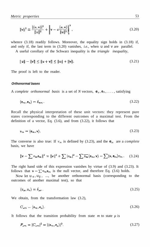
Metric properties 53
(3.20)
whence (3.18) readily follows. Moreover, the equality sign holds in (3.18) if,and only if, the last term in (3.20) vanishes, i.e., when u and v are parallel.
A useful corollary of the Schwarz inequality is the triangle inequality,
(3.21)
The proof is left to the reader.
Orthonormal bases
A complete orthonormal basis is a set of N vectors, ea , eb , . . . , satisfying
(3.22)
Recall the physical interpretation of these unit vectors: they represent purestates corresponding to the different outcomes of a maximal test. From thedefinition of a vector, Eq. (3.6), and from (3.22), it follows that
(3.23)
The converse is also true: If vm is defined by (3.23), and the em are a completebasis, we have
(3.24)
The right hand side of this expression vanishes by virtue of (3.9) and (3.23). Itfollows that is the null vector, and therefore Eq. (3.6) holds.
Now let u α , uβ , ..., be another orthonormal basis (corresponding to theoutcomes of another maximal test), so that
(3.25)
We obtain, from the transformation law (3.2),
(3.26)
It follows that the transition probability from state m to state µ is
(3.27)

54 Complex Vector Space
In particular, as shown below, it is possible to construct orthonormal baseswhich satisfy P µ m = 1/N, for all µ and m. These bases are “as different aspossible” and are called mutually unbiased. For example, in the case of polarizedphotons, a test for vertical vs horizontal linear polarization, a test for the twooblique polarizations at ±45°, and one for clockwise vs counterclockwise circularpolarization, are mutually unbiased. A photon, having passed one of these tests,and then submitted to any other one, has equal chances for yielding the twopossible outcomes of the second test. Some examples of unbiased bases weregiven in Exercise 2.12. It can be shown that, if N is prime, it is always possibleto find N +1 mutually unbiased bases.4,5
The simplest case of unbiased bases results from a discrete Fourier transform:
(3.28)
Quantum tests satisfying (3.28) are called complementary. 6 We shall see inChapter 10 that these tests are the quantum analogs of measurements of clas-sical, canonically conjugate, dynamical variables.
3-3 . Quantum expectation rule
The correspondence between complex vectors and physical pure states is notone to one: Quantum theory considers vectors that are parallel to each otheras representing the same physical state. It is often convenient to normalizevectors by dividing them by their norm, so that the new norm is 1. Therestill remains an arbitrariness of the phase, because v and e iθ v have the samenorm, for any real θ. This phase arbitrariness is an essential feature of quantumtheory. It cannot be eliminated, because of the superposition principle: Givenany two states u and v , the linear combinations u + v and u + e iθ v are physicallyrealizable states, and are not equivalent, as shown by the simple example of thepolarization states of photons, illustrated in Fig. 1.4.
If parallel vectors represent the same physical state, what is the meaning oforthogonal vectors? The latter can be members of an orthogonal basis. Thissuggests the following extrapolation of the principle of superposition G:
G*. Strong superposition principle. Any orthogonal basisrepresents a realizable maximal test.
That is, not only can any individual vector, such as v in Eq. (3.6), be exper-imentally realized, but any complete set of mutually orthogonal vectors has aphysical realization, in the form of a maximal quantum test.
4 I. D. Ivanovic, J. Phys. A 14 (1981) 3241.5 W. K. Wootters, Found. Phys. 16 (1986) 391.6 J. Schwinger, Proc. Nat. Acad. Sc. 46 (1960) 570..

Quantum expectation rule 55
Orthogonal states corresponding to different outcomes of a maximal test arethe quantum analog of “different states” in classical physics. If we definitelyknow that a system has been prepared in one of several given orthogonal states(not in a linear combination thereof) we can unambiguously identify that state,by the appropriate maximal test.
Non-orthogonal states
The generic case is a pair of vectors that are neither parallel nor orthogonal.These vectors correspond to physical states that are neither identical, nortotally different, but “partly alike.” For example, photons with linear polariza-tions tilted at an angle a from each other are partly alike. There is a probabilitycos² α that a photon prepared with one of these linear polarizations will suc-cessfully pass a test for the other linear polarization.
This partial likeness is not peculiar to quantum physics. In the classical phasespace too, we may have Liouville densities, f1 (q, p ) and f 2(q, p ), which partlyoverlap. For example, there may be two different methods for releasing a givenpendulum. In each one of these methods, the initial coordinates and momentaare not controlled with absolute precision; therefore the phase space domainscorresponding to these two different preparation procedures have a finite size.They may be disjoint, or they may partly overlap, as shown in Fig. 3.1. Notethat this figure represents our imperfect knowledge of the classical q and p of asingle pendulum. The use of Liouville densities for representing this imperfectknowledge has the following meaning: We imagine the existence of an infiniteset of identical replicas of our pendulum (that is, we imagine an ensemble, asexplained in Sect. 2-1). All these conceptual replicas are produced according
Fig. 3.1. The results of two different classical preparation procedures areshown by hatchings with opposite orientations. The size of the ellipse repre-sents the expected instrumental error. (a) If the ellipses do not overlap, anobserver can deduce with certainty which method was used. (b) If there isan overlap, it is only possible to assign probabilities to the two methods.

56 Complex Vector Space
to one of the two imperfectly controlled preparation procedures, and all theresulting q and p are therefore represented by a cloud of points in phase space.The density of points in this cloud is the Liouville density, f1 (q, p ) or f 2( q, p ),which corresponds to the preparation method that was used.
Suppose now that an observer wants to determine which one of the twopreparations was actually implemented. Even if that observer is capable ofexactly locating q and p by means of ideal measurements, he may not be ableto tell with certainty to which “cloud” the result belongs. The answer can bestated only in terms of probabilities.
The new feature introduced by quantum theory is that the probabilisticnature of the outcome of a measurement is not due to imperfections of thepreparing or measuring apparatuses. It is inherent to quantum physics. A purequantum state is similar to a classical ensemble. 7 Therefore, the meaningfulquestions are not about the values of dynamical variables, but rather about theprobability that some particular preparation was used. This is a much sounderapproach: quantum dynamical variables are abstract concepts, existing only inour mind. The experimental preparations exist in the laboratory.
Probability interpretation
In general, let us define a “test for state v ” as one which always succeeds forquantum systems prepared in state v, and always fails for those prepared inany state orthogonal to v . This need not be a maximal test, but only onethat singles out v from all the states orthogonal to v . A fundamental result ofquantum theory is the following rule:
H. Quantum expectation rule. Let u and v be two normalizedvectors. The probability that a quantum system prepared in stateu will pass successfully a test for state v is ⟨u, v⟩ ².
With the notations of Sect. 2-4, this means that
Pvu = ⟨ u, v ⟩ ²,
which is an obvious corollary of Eq. (3.27) and of the strong superpositionprinciple G*. (If we had not already assumed the validity of G*, we would haveto consider H as a new, independent postulate.)8
The law of reciprocity D , expressed by Eq. (2.4), now becomes a trivialconsequence of the Hermitian nature of the scalar product (3.14). Conversely,if the reciprocity law D were experimentally falsified, we would have to rejectthe expectation rule H , and then the entire complex vector formalism proposedhere would be devoid of physical interpretation.
(3.29)
7I. R. Senitzky, Phys. Rev. Lett. 47 (1981) 1503.8From postulate G*, together with reasonable continuity assumptions, it is possible to derive
Gleason’s theorem (see Sect. 7-2). That theorem generalizes the quantum expectation rule tostates which are not pure.

Physical implementation 57
3-4. Physical implementation
It is the probability rule H which allows us to relate the abstract mathematicalformalism of quantum theory to actual observations that may be performed ina laboratory. This rule can be derived from previously proposed postulates.Every step in its derivation is a plausible extension of preceding steps. Whenwe retrace the route that was followed in the derivation of H , the weakest linkis the law of composition of transitions amplitudes (Postulate F , page 40) whichmay be no more than an educated guess, influenced by our familiarity withclassical field theory.
Quantum theory, for which we are now collecting appropriate tools, maysome day be found unsatisfactory, and replaced by a more elaborate theory(just as Newtonian mechanics was superseded by special relativity, and then bygeneral relativity theory). The need to discard—or upgrade—quantum theorymay arise when we become able to probe smaller spacetime regions, or strongergravitational fields, or biological systems, or other phenomena yet unforeseen.However, a more urgent task is to check the theory for internal consistency.All the foregoing discussion involved ideal maximal tests, which can only beroughly approximated by real laboratory procedures. The final chapter of thisbook will be devoted to the “measurement problem.” It will give a more detaileddescription of the experimenter’s work with quantum systems. At the presentstage, I shall only propose another version of the expectation rule, with a mildoperational flavor:
I . Quantum expectation rule (operational version). For anytwo normalized vectors u and v, it is possible to design experimentaltesting procedures with the following property: a quantum systemwhich certainly passes the test for state u has a probability ⟨u,v⟩ ²to pass the test for state v , and vice versa.
This new version is more explicit than H , but not yet fully satisfactory. Aquantum test is not a supernatural event. It is a physical process, involvingordinary matter. Our testing instruments are subject to the ordinary physicallaws. If we ignore this obvious fact and treat quantum tests as a primitivenotion, as we are presently doing, we are guilty of a gross oversimplification ofphysics. We shall return to this problem in Chapter 12. Meanwhile, let us notethat the consistency of the expectation rule implies that dynamical laws musthave specific properties:
J. Dynamical description of quantum tests. Let U and Vdenote apparatuses which perform the tests for states u and v ,respectively. The dynamical laws which govern the working of theseapparatuses must have the following property: If quantum systemsare prepared in such a way that apparatus U always indicates asuccessful test, apparatus V has a probability ⟨u, v⟩ ² to yield apositive answer, and vice versa.

58 Complex Vector Space
It is not obvious that this requirement can be fulfilled for arbitrary u and v .Dynamical laws cannot be decreed by whim, without risking a violation ofphysical principles that we wish to respect, such as conservation of charge, orrelativistic invariance, or the second law of thermodynamics. More often thannot, it is impossible to satisfy condition J in a rigorous way (as will be seen inChapter 12), but it still can be satisfied to an arbitrarily good approximation.
In last resort, the fundamental question is: What distinguishes a quantumtest from any other dynamical process governed by quantum theory? Thecharacteristic property of a genuine test is that it produces a permanent record,which can be described by our ordinary language, after having been observed byordinary means, without the risk of being perturbed by the act of observation.It does not matter whether someone will actually observe this record. It issufficient to prove, by relying on known physical laws, that an observation is inprinciple possible and can be repeated at will by several independent physicistswithout giving rise to conflicting results. In summary, the outcome of a test isan objective event (some authors prefer the term intersubjective ).
The robustness of a macroscopic record—its stability with respect to smallperturbations such as those caused by repeated observations—suggests thatirreversible processes must be involved. This is a complicated issue, not yetfully understood, which will be discussed in Chapter 11.
Having thus warned the reader of the difficulties lying ahead, I now return tothe formal and naive approach where a quantum test is an unexplained event,producing a definite and repeatable outcome, in accordance with well definedprobability rules given by quantum theory.
3-5 . Determination of a quantum state
Suppose that the only information we have about a preparation procedure isthat it produces a pure state. (The more general case of mixed states will bediscussed later.) Our task is to determine the components of the correspondingstate vector, If we can prepare and test anunlimited number of systems, it follows from the expectation rule H that wecan measure, with arbitrary accuracy, the probabilities of outcomes such as
or (3.30)
There are 2(N – 1) independent experimental data in (3.30), because of theconstraints . This is exactly the number of data that weneed to determine the phases of these complex numbers. Indeed, let us write
(3.31)
where r m and φm are real. Note that the phases φm are defined only up to anarbitrary common additive constant. The N moduli r m are given by the first
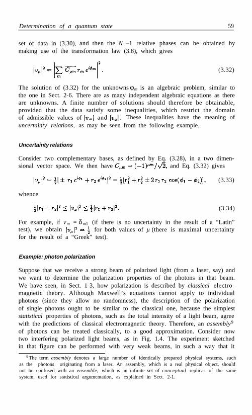
Determination of a quantum state 59
set of data in (3.30),and then the N –1 relative phases can be obtained bymaking use of the transformation law (3.8), which gives
(3.32)
The solution of (3.32) for the unknownsφm is an algebraic problem, similar tothe one in Sect. 2-6. There are as many independent algebraic equations as thereare unknowns. A finite number of solutions should therefore be obtainable,provided that the data satisfy some inequalities, which restrict the domainof admissible values of and . These inequalities have the meaning ofuncertainty relations, as may be seen from the following example.
Uncertainty relations
Consider two complementary bases, as defined by Eq. (3.28), in a two dimen-sional vector space. We then have and Eq. (3.32) gives
whence
(3.33)
(3.34)
For example, if vm = δm1 (if there is no uncertainty in the result of a “Latin”test), we obtain for both values of µ (there is maximal uncertaintyfor the result of a “Greek” test).
Example: photon polarization
Suppose that we receive a strong beam of polarized light (from a laser, say) andwe want to determine the polarization properties of the photons in that beam.We have seen, in Sect. 1-3, how polarization is described by classical electro-magnetic theory. Although Maxwell’s equations cannot apply to individualphotons (since they allow no randomness), the description of the polarizationof single photons ought to be similar to the classical one, because the simpleststatistical properties of photons, such as the total intensity of a light beam, agreewith the predictions of classical electromagnetic theory. Therefore, an assembly9
of photons can be treated classically, to a good approximation. Consider nowtwo interfering polarized light beams, as in Fig. 1.4. The experiment sketchedin that figure can be performed with very weak beams, in such a way that it
9The term assembly denotes a large number of identically prepared physical systems, suchas the photons originating from a laser. An assembly, which is a real physical object, shouldnot be confused with an ensemble, which is an infinite set of conceptual replicas of the samesystem, used for statistical argumentation, as explained in Sect. 2-1.

60 Complex Vector Space
is unlikely to have at any moment more than one photon in the apparatus;and nevertheless, the total number of photons during the entire experiment isvery large, so that the laws of classical optics must be valid. This two-sidedsituation suggests that we represent the polarization states of a single photonby a linear space, like the one used in classical electrodynamics. This conclusionis of course in complete agreement with the superposition principle G.
Note that, in the present discussion, we are concerned only with polarizationproperties. The number of photons—i.e., the beam intensity—and the locationof that beam are not considered. In other words, the “quantum system” thatwe are testing by calcite crystals and similar devices is only the polarization of aphoton. (Recall the discussion of the Stern-Gerlach experiment in Sect. l-5: the“quantum system” was the magnetic moment µ of a silver atom. The positionof the atom could be described classically.)
The linear space describing photon polarization is two-dimensional, becausethere are two distinct states corresponding to each maximal test; and it is acomplex space, because phase relationships are essential (see Fig. 1.4). We arethus led to a representation of polarization states by column vectors , withcomplex components α and β , satisfying the normalization condition
(3.35)
The two outcomes of any maximal test may be taken as a basis for this two-dimensional linear space. Different tests correspond to different bases, as wehave seen. For example, the vectors ex = and e y = can be taken torepresent linear polarizations in the x- and y -directions, respectively.
The classical superposition principle (1.3) suggests that α ∼ Ex exp(i δx )and β ~ E δy exp(i y ), with a proportionality constant which depends on theunits chosen and on the intensity of the beam, and which in any case includesthe common phase e i(kz– ωt ) . Here, E x and E y can be taken as functions of xand y , if we wish to represent beams of finite extent, rather than an infiniteplane wave. Note that the polarization of a light beam depends only on theratio of the components E x and E y , and on their relative phase. Multiplyingboth components by the same number does not change the polarization of thelight beam, but only its total intensity.
Suppose now that a photon with unknown polarization is tested forlinear polarization in a direction making an angle θ with the x-axis. We knowthat a classical electromagnetic wave will pass without reduction of intensityif E x /Ey = cos θ / sin θ . It follows that photons with that polarization state,
, always pass the test. Likewise, those having the orthogonal
polarization, namely , always fail the test. In general, we canwrite
(3.36)
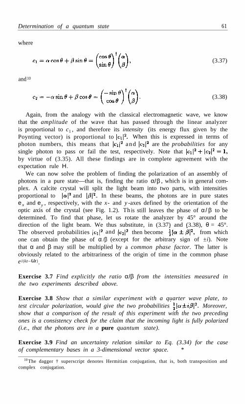
Determination of a quantum state 61
where
and10
(3.37)
(3.38)
Again, from the analogy with the classical electromagnetic wave, we knowthat the amplitude of the wave that has passed through the linear analyzeris proportional to c1 , and therefore its intensity (its energy flux given by thePoynting vector) is proportional to . When this is expressed in terms ofphoton numbers, this means that and are the probabilities for anysingle photon to pass or fail the test, respectively. Note thatby virtue of (3.35). All these findings are in complete agreement with theexpectation rule H.
We can now solve the problem of finding the polarization of an assembly ofphotons in a pure state—that is, finding the ratio α/β , which is in general com-plex. A calcite crystal will split the light beam into two parts, with intensitiesproportional to and . In these beams, the photons are in pure statese x and ey , respectively, with the x- and y -axes defined by the orientation of theoptic axis of the crystal (see Fig. 1.2). This still leaves the phase of α/ β to bedetermined. To find that phase, let us rotate the analyzer by 45° around thedirection of the light beam. We thus substitute, in (3.37) and (3.38), θ = 45°.The observed probabilities and then become from whichone can obtain the phase of α /β (except for the arbitrary sign of ±i). Notethat α and β may still be multiplied by a common phase factor. The latter isobviously related to the arbitrariness of the origin of time in the common phaseei (kz–ωt ).
Exercise 3.7 Find explicitly the ratio α/β from the intensities measured inthe two experiments described above.
Exercise 3.8 Show that a similar experiment with a quarter wave plate, totest circular polarization, would give the two probabilities Moreover,show that a comparison of the result of this experiment with the two precedingones is a consistency check for the claim that the incoming light is fully polarized(i.e., that the photons are in a pure quantum state).
Exercise 3.9 Find an uncertainty relation similar to Eq. (3.34) for the caseof complementary bases in a 3-dimensional vector space. *
10The dagger † superscript denotes Hermitian conjugation, that is, both transposition andcomplex conjugation.

62 Complex Vector Space
Exercise 3.10 Four polarization filters are introduced in a Mach-Zehnderinterferometer, as shown in the figure below. The two internal filters allow thepassage of light with vertical and horizontal polarization, respectively. The filternear the source is oblique, at 45°. The filter near the observer may be rotated,or removed. Show that no interference fringes will appear if the observer’s filteris vertical, or horizontal, or absent. On the other hand, there will be fringesif that filter is oblique. How can the existence of these fringes be explained interms of polarized photons travelling in the interferometer? What happens tothese fringes if the filter near the source is removed, or is rotated to the verticalor horizontal position?
Fig. 3.2. Mach-Zehnder interferometer with four polarizationfilters. (This experiment was suggested by M. E. Burgos.)
3-6. Measurements and observables
A meaningful quantum test must have a theoretical interpretation, usually for-mulated in the language of classical physics. For example, if a Stern-Gerlachtest is found to have three distinct outcomes for a given atomic beam, we in-terpret these outcomes as the values µ , 0, and –µ, which can be taken by acomponent of the magnetic moment of each atom. In the absence of obviousclassical values for the outcomes of a test, we may ascribe arbitrary numericallabels to these outcomes; for example, in Fig. 1.3, the two linear polarizationscan be labelled ±1. Thus, in general, we associate N real numbers, a1, . . . , a N,with the N distinct outcomes of a given maximal test.
Once this has been done, we may say that the result of a quantum testis a real number, and the test becomes similar to a classical measurement,which also yields a number. I shall therefore follow the usage and call thattest a “quantum measurement.” However, as explained in Sect. 1-5, this newtype of measurement is not a passive acquisition of knowledge, as in classicalphysics. There is no “physical quantity” whose value is unknown before the
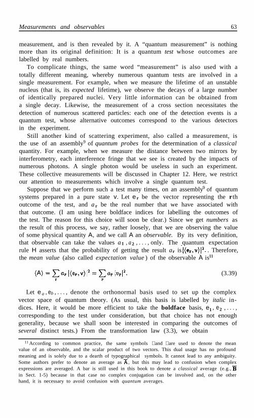
Measurements and observables 63
measurement, and is then revealed by it. A “quantum measurement” is nothingmore than its original definition: It is a quantum test whose outcomes arelabelled by real numbers.
To complicate things, the same word “measurement” is also used with atotally different meaning, whereby numerous quantum tests are involved in asingle measurement. For example, when we measure the lifetime of an unstablenucleus (that is, its expected lifetime), we observe the decays of a large numberof identically prepared nuclei. Very little information can be obtained froma single decay. Likewise, the measurement of a cross section necessitates thedetection of numerous scattered particles: each one of the detection events is aquantum test, whose alternative outcomes correspond to the various detectorsin the experiment.
Still another kind of scattering experiment, also called a measurement, isthe use of an assembly9 of quantum probes for the determination of a classicalquantity. For example, when we measure the distance between two mirrors byinterferometry, each interference fringe that we see is created by the impacts ofnumerous photons. A single photon would be useless in such an experiment.These collective measurements will be discussed in Chapter 12. Here, we restrictour attention to measurements which involve a single quantum test.
Suppose that we perform such a test many times, on an assembly9 of quantumsystems prepared in a pure state v. Let e r be the vector representing the r thoutcome of the test, and a r be the real number that we have associated withthat outcome. (I am using here boldface indices for labelling the outcomes ofthe test. The reason for this choice will soon be clear.) Since we get numbers asthe result of this process, we say, rather loosely, that we are observing the valueof some physical quantity A, and we call A an observable. By its very definition,that observable can take the values a 1 , a 2 , . . . ,only. The quantum expectationrule H asserts that the probability of getting the result ar is . Therefore,the mean value (also called expectation value ) of the observable A is11
(3.39)
Let e a , eb , . . . , denote the orthonormal basis used to set up the complexvector space of quantum theory. (As usual, this basis is labelled by italic in-dices. Here, it would be more efficient to take the boldface basis, e1 , e2 , . . . ,corresponding to the test under consideration, but that choice has not enoughgenerality, because we shall soon be interested in comparing the outcomes ofseveral distinct tests.) From the transformation law (3.3), we obtain
11According to common practice, the same symbols ⟨ and ⟩ are used to denote the meanvalue of an observable, and the scalar product of two vectors. This dual usage has no profoundmeaning and is solely due to a dearth of typographical symbols. It cannot lead to any ambiguity.Some authors prefer to denote an average as , but this may lead to confusion when complexexpressions are averaged. A bar is still used in this book to denote a classical average (e.g.,in Sect. 1-5) because in that case no complex conjugation can be involved and, on the otherhand, it is necessary to avoid confusion with quantum averages.

64 Complex Vector Space
(3.40)
This can also be written as
(3.41)
clearly showing the distinct roles of the expressionsvm vn , which refers solelyto the preparation of the quantum system being tested, and
(3.42)
which refers solely to the quantum test defining the basis er , and thereby theobservable A.
An observable is therefore represented by a matrix in our complex vectorspace. These matrices will be denoted by capital sans serif letters, such as A,to distinguish them from ordinary complex numbers, such as their componentsA mn . The Hermitian conjugate of a matrix, denoted by a superscript† , isdefined as the complex conjugate transposed matrix:
(3.43)
Since ar is real, it follows from (3.42) that Am n = An m , so that any observablematrix is Hermitian: A = A†. It will be shown later that the converse is alsotrue: any Hermitian matrix defines an observable.
Transformation properties
Note that we have now two essentially different types of matrices. There areunitary transformation matrices, such as Cµ m or C rm , whose indices belong totwo different alphabets, indicating that they refer to two different orthogonalbases; and there are Hermitian matrices, like Am n , which represent observablephysical properties, described with the use of a single basis.
It is natural to ask what is the transformation law of the components of theseobservable matrices, when we refer them to another basis. For example, we maydefine, by analogy with (3.42), the expression
(3.44)
where the transformation matrix Γ is defined by Eq. (3.3). These transformationmatrices are not independent (in mathematical parlance, they form a group) .Inserting the composition law (3.4) into (3.42), we obtain
(3.45)

Measurements and observables 65
whence, by comparing with (3.44),
(3.46)
This is the transformation law for observable matrices. It is similar to the vectortransformation law (3.8), but now both Cµm and its complex conjugate appear,because the transformed elements have two indices.12
Exercise 3.11 Derive (3.46) from (3.8) and from the requirement that
(3.47)
gives a result which agrees with Eq. (3.41).
Exercise 3.12 Show that
(3.48)
I shall now show that the N expressions w m = ∑ n Am n v n are the componentsof a vector which can be written as w = Av. This is not a trivial claim because,in general, N arbitrary numbers are not the components of a vector. Thecharacteristic property of a vector is that its components obey a well definedtransformation law (the same law for all vectors!) when these components arereferred to another basis. Simple examples of non-vectors are shown in thefollowing exercises:
Exercise 3.13 A vector x1 , x 2 in the Euclidean plane is defined by theproperty that a rotation of the axes by an angle q induces a linear mapping
(3.49)
Show that the pair of numbers y1 , y 2 = x1, –x2 also has a linear mappinglaw under a rotation of the axes, but that law has not the same form as (3.49)and therefore the pair y1 , y 2 is not a vector. On the other hand, show that u 1 , u2 = – x2, x 1 transforms according to
(3.50)
and therefore the pair u1 ,u2 is a vector.
12 If you are familiar with general relativistic notations, and in particular with spinor theoryin curved spaces, you will want to introduce here lower (covariant) and upper (contravariant)indices, as well as dotted and undotted indices for complex conjugate transformations. I refrainfrom using these exquisite notations, lest they scare the uninitiated.

66 Complex Vector Space
Exercise 3.14 Show that the pair of numbersbehaves, under the mapping (3.50), as a vector would have behaved under arotation of the axes by an angle 2θ, rather than θ. Therefore, v1 and v2 are notthe components of a vector (they are the components of a tensor ) .
Let us therefore examine whether w = Av is a vector: We must find whathappens to the equation wm = ∑ n A mn vn , when that equation is referred toanother orthonormal basis—say eµ . Sha l l we then ge t w µ = ∑ v Aµv vv , withwµ satisfying the transformation law (3.8)? The answer is positive, as may beseen from the transformation laws (3.8) and (3.46). These give
and this is indeed wm . This formally proves that the components of w transformlike those of a vector. In other words, an observable matrix is a linear operatormapping vectors into vectors.
Once this point is established, we can considerably simplify the notation anddiscard all the indices (Latin, Greek, boldface, etc.) which refer vectors tovarious orthogonal bases. For example, Eq. (3.41) becomes
(3.51)
This symbolic notation is not only aesthetically more pleasant; it will be theonly possible one for infinite dimensional vector spaces, where “indices” takecontinuous values (see Chapter 4). The index free notation is unambiguousprovided that all vectors and matrices are referred to the same basis. Explicitindexing is preferable when transformations among several bases are involved.
Projection operators
The simplest observables are those for which all the coefficients ar are either 0or 1. These observables correspond to tests which ask yes-no questions (yes = 1,no = 0). They are called projection operators , or simply projectors , for thefollowing reason: For any normalized vector v, one can define a matrix P v = vv †,with the properties Pv ² = P v and
(3.52)
The last expression is a vector parallel to v , for any u , unless ⟨ v,u ⟩ = 0. Ingeometric terms, Pvu is the projection of u along the direction of v. Projectorsof a more general type than in Eq. (3.52) will be discussed later.
These projection operators are very handy. In particular, we can write anyobservable A as a linear combination of projectors on the basis which definesthat observable:
(3.53)
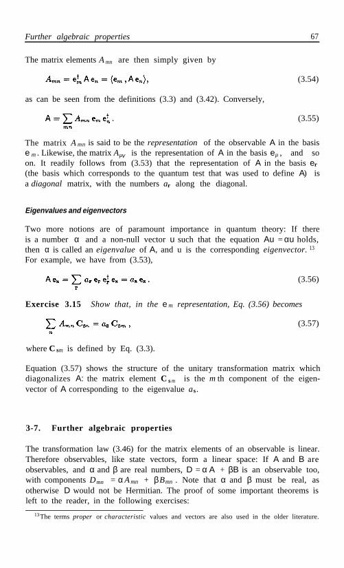
Further algebraic properties 67
The matrix elements A mn are then simply given by
(3.54)
as can be seen from the definitions (3.3) and (3.42). Conversely,
(3.55)
The matrix A mn is said to be the representation of the observable A in the basise m . Likewise, the matrix Aµv is the representation of A in the basis eµ , and soon. It readily follows from (3.53) that the representation of A in the basis er
(the basis which corresponds to the quantum test that was used to define A) isa diagonal matrix, with the numbers ar along the diagonal.
Eigenvalues and eigenvectors
Two more notions are of paramount importance in quantum theory: If thereis a number α and a non-null vector u such that the equation Au = αu holds,then α is called an eigenvalue of A, and u is the corresponding eigenvector. 13
For example, we have from (3.53),
(3.56)
Exercise 3.15 Show that, in the e m representation, Eq. (3.56) becomes
(3.57)
where C sm is defined by Eq. (3.3).
Equation (3.57) shows the structure of the unitary transformation matrix whichdiagonalizes A: the matrix element C s m is the m th component of the eigen-vector of A corresponding to the eigenvalue as.
3-7. Further algebraic properties
The transformation law (3.46) for the matrix elements of an observable is linear.Therefore observables, like state vectors, form a linear space: If A and B areobservables, and α and β are real numbers, D = α A + βB is an observable too,with components Dmn = α A mn + βBmn . Note that α and β must be real, asotherwise D would not be Hermitian. The proof of some important theorems isleft to the reader, in the following exercises:
13The terms proper or characteristic values and vectors are also used in the older literature.

68 Complex Vector Space
Exercise 3.16 Show that if C is unitary and A is Hermitian, C †AC is alsoHermitian. Likewise if U is unitary, C†UC is unitary.
Exercise 3.17 Show that any algebraic relation between matrices, suchas A + B = D, or AB = D, is invariant under a similarity transformationA → S – 1AS, B → S–1 BS (and in particular under a unitary transformation).
Nonlinear functions of an observable are defined by the natural generalizationof Eq. (3.53):
(3.58)
Their matrix elements are given as in (3.42):
(3.59)
For the integral powers of an observable, this definition coincides with raisingits matrix to the same power. For example,
(3.60)
is indeed equal to , by virtue of (3.1). However, the definition(3.58) is also applicable to functions which cannot be expanded into powerseries, such as log A. Note that if the function ƒ is bijective, the measurementsof A and ƒ(A) are equivalent, in the sense of Postulate B (page 31).
Exercise 3.18 Show that if H is Hermitian, ei H is unitary.
Exercise 3.19 Show that if U is unitary, i( – U)/( + U) is Hermitian.(Here, denotes the unit matrix.)
Next, let us consider functions of several observables—A and B, say—whichare not defined by the same complete test. While A is defined as above byassociating real numbers a r with a set of orthonormal vectors e r , one definesB by associating real numbers b µ with another set of orthonormal vectors, eµ ,corresponding to a different maximal test. (If you want a concrete example,think of A and B as angular momentum components, Jx and J y .) As before,we refer all the components of vectors and matrices to some fixed orthonormalbasis em (for example, the one in which J z is diagonal). The matrix Amn isgiven by Eq. (3.42), and likewise we have
(3.61)
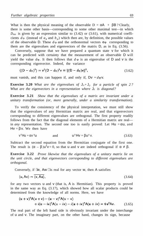
Further algebraic properties 69
What is then the physical meaning of the observable D = αA + βB ? Clearly,there is some other basis—corresponding to some other maximal test—in whichDmn is given by an expression similar to (3.42) or (3.61), with numerical coeffi-cients d (instead of a r and b µ ) which then are, by definition, the possible valuesof the observable D. These d and the orthonormal vectors e corresponding tothem are the eigenvalues and eigenvectors of the matrix D, as in Eq. (3.56).
Conversely, suppose that we have prepared a quantum state v for which itcan be predicted with certainty that the measurement of an observable D willyield the value d . It then follows that d is an eigenvalue of D and v is thecorresponding eigenvector. Indeed, the variance
(3.62)
must vanish, and this can happen if, and only if, Dv = d v.
Exercise 3.20 What are the eigenvalues of Jx + Jy for a particle of spin 2 ?What are the eigenvectors in a representation where Jz is diagonal?
Exercise 3.21 Show that the eigenvalues of a matrix are invariant under aunitary transformation (or, more generally, under a similarity transformation).
To verify the consistency of the physical interpretation, we must still showthat the eigenvalues of any Hermitian matrix are real, and that eigenvectorscorresponding to different eigenvalues are orthogonal. The first property readilyfollows from the fact that the diagonal elements of a Hermitian matrix are real—in any representation. The second one too is easily proved: Let Hu = αu, andHv = βv. We then have
v†Hu = αv †u and u†Hv = βu† v. (3.63)
Subtract the second equation from the Hermitian conjugate of the first one.The result is (α – β )u†v = 0, so that u and v are indeed orthogonal if α ≠ β.
Exercise 3.22 Prove likewise that the eigenvalues of a unitary matrix lie onthe unit circle, and that eigenvectors corresponding to different eigenvalues areorthogonal.
Conversely, if ⟨ w, Aw ⟩ is real for any vector w, then A satisfies
(3.64)
for any two vectors u and v (that is, A is Hermitian). This property is provedin the same way as Eq. (3.17), which showed how all scalar products could bedetermined from the knowledge of all norms. Here, we have
(3.65)
The real part of the left hand side is obviously invariant under the interchangeof u and v. The imaginary part, on the other hand, changes its sign, because

70 Complex Vector Space
(3.66)
and Eq. (3.64) readily follows.
Computation of eigenvalues and eigenvectors
To obtain explicitly the eigenvalues and eigenvectors of a given matrix A, wehave to solve ∑ Amn un = α u n , or ∑ ( Am n – αδm n )un = 0. These linear equa-tions have a nontrivial solution if, and only if, Det (Amn – α δmn ) = 0. This isan algebraic equation of order N, called the secular equation. If α is a simpleroot of this equation, the corresponding eigenvector is obtained by solving a setof linear equations, and it is unique, up to a normalization factor.
If the same eigenvalue occurs more than once, it is called “degenerate,” andit may have several independent eigenvectors. In particular, if A is Hermitian(or unitary), it is always possible to construct M orthonormal eigenvectorscorresponding to an M-fold root of the secular equation. This can be provedas follows. We first find one eigenvector, v say. We then perform a unitarytransformation to a new basis, such that v is the kth basis vector. This doesnot affect the eigenvalues of A (see Exercise 3.21). In the new basis, we have∑ A mn vn = α vm . However, in that basis, the only nonvanishing component ofv is v k , whence it follows that A k k = α and all the other A mk = 0, and thereforeall A km = 0 too, because A is Hermitian. Consider now a new matrix A’ whichis the same as A , but with the k th row and column removed. This matrix isdefined in the subspace of all the vectors orthogonal to v. By construction, itseigenvectors are also eigenvectors of A, with the same eigenvalues. Repeatingthis process M – 1 times, we can find M orthogonal eigenvectors pertaining tothe M -fold eigenvalue. Obviously, any linear combination of these vectors is alsoan eigenvector, corresponding to the same eigenvalue. Additional informationcan be found in texts on algebra, such as those listed in the bibliography.
Exercise 3.23 Prove that similar properties hold for unitary matrices.
Exercise 3.24 On the other hand, show that the matrix , which is
neither Hermitian nor unitary, has only a single eigenvector.
Exercise 3.25 Show that the trace (the sum of diagonal elements) of aHermitian—or unitary—matrix is equal to the sum of its eigenvalues, and thedeterminant of that matrix is equal to the product of its eigenvalues.
From the definition of f (A)—see Eq. (3.53)—it readily follows that if allthe eigenvalues a r satisfy a relationship f (ar ) = 0, then f (A ) = 0 too. Theconverse is also true, as can be seen by considering the representation where Ais diagonal. A simple example is that of projection operators (or projectors) ,for which all eigenvalues are either 0 or 1, and which therefore satisfy

Further algebraic properties 71
P² = .P (3.67)
Exercise 3.26into the sum of two orthogonal terms:
Prove that any projector P can be used to split any vector v
(3.68)
Exercise 3.27 Let u and v be normalized vectors. Show that uu† and vv†
are projectors. Moreover, show that u u† + vv† is a projector if, and only if,⟨u, v⟩ = 0. Generalize this result to an arbitrary number of vectors.
Exercise 3.28 Let eµ be a complete orthogonal basis. Show that
(3.69)
where is the unit matrix.
Commutators
The expression
(3.70)
is called the commutator of the matrices A and B. If [A, B] = 0, we say thatA and B commute. Obviously, two observables defined by means of the samemaximal test commute (there is a representation in which both are diagonal).Conversely, if A and B are Hermitian and commute, it is possible to find a basiswhere both matrices are diagonal. This can be done as follows: First, let usdiagonalize A. We then have
(3.71)
If A is nondegenerate, it follows that B mn = 0 whenever m ≠ n ( i.e. , B toois diagonal). If, on the other hand, A is degenerate, B is only block-diagonal.Each one of the blocks corresponds to a set of equal eigenvalues of A (that is,the corresponding block of A is a multiple of the unit submatrix). We can thendiagonalize each block of B separately without affecting A, so that, finally, bothA and B are diagonal.
In particular, consider two projectors P and Q. If they commute, both can bediagonalized in some basis. In that case, their product PQ = QP has diagonalelements equal to 1 only where both P and Q have such diagonal elements.Projection operators which satisfy PQ = 0 are said to be orthogonal.
Exercise 3.29 Show that if the projection operators P and Q satisfy PQ = 0,then QP = 0 too.

72 Complex Vector Space
Exercise 3.30 Show that if P and Q are orthogonal projectors, and v is anyvector, ⟨ Pv, Qv ⟩ = 0.
Exercise 3.31 Show that if P is a projector, the operator – P is also aprojector, and it is orthogonal to P.
Normal matrices and polar decomposition
To conclude this brief tour of linear algebra, here are two more definitions. Amatrix A is called normal if it commutes with its adjoint: [A, A†] = 0. Inthat case, the Hermitian matrices A + A† and i (A – A† ) commute and can besimultaneously diagonalized by a unitary transformation. Therefore A itself canbe diagonalized.
Consider now a generic matrix A, which is not normal, and therefore cannotbe diagonalized by a unitary transformation. It may still be possible to writeA in polar form, like we write a complex number z = reiθ. Indeed, the matrixA†A is Hermitian, and it has nonnegative eigenvalues, because, for any u,
(3.72)
Further assume that A†A has no zero eigenvalue (i.e., the equation Au = 0 hasno solution other than u = 0). Since A†A is Hermitian, it is possible to define,thanks to Eq. (3.58), the matrix (A†A) – ½, where, for definiteness, we choosethe positive square root of each eigenvalue of A†A. Then, the matrix product
(3.73)
is unitary, because , and we finally have
(3.74)
The reader is invited to work out an explicit example, such asand to see what happens in the limit ∈ → 0.
3-8 . Quantum mixtures
Most tests are not maximal and most preparations do not produce pure quan-tum states. We often have only partial specifications for a physical process. Wetherefore need a formalism for describing incompletely specified situations.
Imagine a procedure in which we prepare various pure states uα , with re-spective probabilities pα . The vectors u α are normalized but not necessarilyorthogonal to each other. The corresponding projectors are (a newsymbol ρα was introduced here, instead of the former Pα , to avoid confusionwith the probabilities pα ).
The average value of an observable A for the pure state uα is

Quantum mixtures 73
(3.75)
where the trace of a matrix is defined as the sum of its diagonal elements.Traces will frequently occur in our calculations. You should be familiar withtheir most important properties, which are listed in the following exercises.
Exercise 3.32 Prove that Tr (αA + βB) = α Tr (A) + β Tr (B).
Exercise 3.33 Prove that Tr(AB ) = Tr(BA ). As a corollary, prove that thetrace of a matrix is invariant under similarity transformations A → SAS-1 . Inparticular, it is invariant under unitary transformations.
Exercise 3.34 Prove that Tr( AB ) is real if A and B are Hermitian.
Returning to our stochastic preparation procedure, where the pure state uαoccurs with probability p α, we get, as the average value of the observable A:
(3.76)
which can be written as
(3.77)
where
(3.78)
is the density matrix (or statistical operator) of the quantum system. It satisfies
(3.79)
Note in particular that = 1, as it ought to be.Equation (3.77)can be considered as a generalization of (3.41) when the
preparation of a system is not completely specified. The notion of densitymatrix—just as that of state vector—describes a preparation procedure; or, ifyou prefer, it describes an ensemble of quantum systems, whose statistical prop-erties correspond to the given preparation procedure. A pure state is a specialcase of Eq. (3.78), when only one of the pα is 1, and all the other ones vanish.In that case, ρ is a projection operator and satisfies
(3.80)
Conversely, if Eqs. (3.79) and (3.80) are satisfied, ρ is a projector on somepure state w. Indeed, (3.80) implies that the eigenvalues of ρ are 0 and 1,and (3.79) that the sum of these eigenvalues is 1. Therefore, there is a singleeigenvector w satisfying ρw = w, and we have ρ = w w†.
Note that any projector satisfies

74 Complex Vector Space
(3.81)
Hence the diagonal elements of a projector are nonnegative, and so are those ofany density matrix. This property cannot be affected by choosing another basis.In particular, the eigenvalues of a density matrix are nonnegative. Moreover,none of these eigenvalues can exceed 1, because of (3.79).
Exercise 3.35 A maximal test defines an orthonormal basis eµ . Show thatthe probability of obtaining the µth outcome of that test, following a preparationρ, is Tr (ρP µ ), where
Positive operators
A positive operator A is defined by the property that ⟨w,Aw⟩ ≥ 0 for anyw (a more accurate name would have been “nonnegative operator”). Such anoperator is always Hermitian, as seen in the proof of Eq. (3.64). It satisfiesfurther interesting inequalities. Consider, for example, a vector v with only twononvanishing components, v m and vn , say. Since v†Av involves only a submatrixof A with elements labelled by the indices m or n, that submatrix itself mustbe a positive operator. In particular, its eigenvalues cannot be negative, andtherefore—see Exercise (3.25)—the corresponding subdeterminant,
, cannot be negative. It follows that if a diagonal element Am m vanishes,the entire m th row and m th column of A must vanish. More generally, if amatrix is positive, then any submatrix, obtained by keeping only the rows andcolumns labelled by a subset of the original indices, is itself a positive matrix,and in particular it has a nonnegative determinant.
Decomposition of a density matrix
An important corollary is that if we try to decompose a pure state ρ = uu† as
(3.82)
with 0 < λ < 1, we can obtain only
(3.83)
Indeed, consider any v orthogonal to u. We have
(3.84)
Since both λ and (1 – λ ) are positive, it follows thatTherefore, if we choose a representation in which both u and v are basis vectors,the entire row and column belonging to v must vanish. It follows that the onlynonvanishing components of ρ´ and ρ '' are = 1, whence weobtain Eq. (3.83).

Quantum mixtures 75
On the other hand, any density matrix which is not a pure state can bedecomposed into pure states in infinitely many ways.14 For example, we have
(3.85)
where the two matrices on the right hand side are projectors on the orthogonalpure states and , respectively. The same diagonal density matrix (3.85)can also be decomposed in an infinity of other ways, such as
(3.86)
where the last two matrices correspond to pure states and which
are orthogonal to each other, but not to or This lack of uniqueness has a remarkable consequence. Given two different
preparations represented by density matrices ρ1 and ρ2 , one can prescribe athird preparation, ρ, as follows: Let a random process have probability λ to“succeed” and probability (1 – λ ) to “fail.” In case of success, prepare thequantum system according to ρ1 . In case of failure, prepare it according to ρ2 .The result is represented by the density matrix
(3.87)
because, if the above instructions are executed a large number of times, theaverage value obtained for subsequent measurements of any observable A is
(3.88)
This property will be expressed as our final fundamental postulate:
What is truly amazing in this result is that, once ρ is given, it contains all theavailable information, and it is impossible to reconstruct from it the original ρ1
and ρ2 ! For example, we may have an experimental setup in which we preparea large number of polarized photons, and we toss a coin to decide, with equalprobabilities, whether the next photon to be prepared will have vertical or hor-izontal linear polarization; or we may have a completely different experimentalsetup, in which we randomly decide whether the next photon will have righthanded or left handed circular polarization. In both cases, we shall get the same
An observer, receiving megajoules of these photons, will never be ableto discover which one of these two methods was chosen for their preparation,notwithstanding the fact that these preparations are macroscopically different.(If he were able to do so, he could use this capability for the instantaneoustransfer of information to distant observers, in violation of relativistic causality.This will be shown in Chapter 6.)
14A quantum mixture is therefore radically different from a chemical mixture, which has aunique decomposition into pure components.
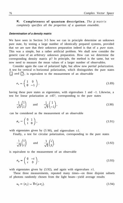
76 Complex Vector Space
K.completely specifies all the properties of a quantum ensemble.
Completeness of quantum description. The ρ matr i x
Determination of a density matrix
We have seen in Section 3-5 how we can in principle determine an unknownpure state, by testing a large number of identically prepared systems, providedthat we are sure that their unknown preparation indeed is that of a pure state.This was a simple, but a rather artificial problem. We shall now consider thegeneric case of an arbitrary unknown preparation. How can we determine thecorresponding density matrix ρ? In principle, the method is the same, but wenow need to measure the mean values of a larger number of observables.
Consider again the case of polarized light, but allow now partial polarization.A test for vertical vs horizontal polarization, which distinguishes the pure states
and , is equivalent to the measurement of an observable
(3.89)
having these pure states as eigenstates, with eigenvalues 1 and –1. Likewise, atest for linear polarization at ±45°, corresponding to the pure states
and (3.90)
can be considered as the measurement of an observable
and (3.92)
is equivalent to the measurement of an observable
(3.91)
with eigenstates given by (3.90), and eigenvalues ±1.Finally, a test for circular polarization, corresponding to the pure states
(3.93)
with eigenstates given by (3.92), and again with eigenvalues ±1.These three measurements, repeated many times—on three disjoint subsets
of photons randomly chosen from the light beam—yield average results
(3.94)

Appendix: Dirac’s notation 77
The observed values of these aj are three experimental data, which, togetherwith the trace condition (3.79), allow us to determine the unknown values ofthe four elements of the Hermitian matrix ρ. The result is
(3.95)
as can easily be verified by using the identity
(3.96)
Exercise 3.36 Show that (3.94) is a consequence of (3.95).
Exercise 3.37 For quantum systems having N orthogonal states, how manydifferent measurements are needed to determine ρ? Ans.: N + 1.
Exercise 3.38 Show that ρ in Eq. (3.95) corresponds to a pure state (thatis, to fully polarized light) if
Exercise 3.39 What are the eigenvalues of ρ in Eq. (3.95)? Ans.: The twoeigenvalues are Therefore, if an experimenter findshe’d better look for systematic errors.
3-9. Appendix: Dirac’s notation
Most notations used in this chapter are the standard ones of linear algebra.They may become awkward when complicated quantum systems have to bedescribed. For example, the state of a free hydrogen atom involves its totalmomentum p , the internal quantum numbers n, l, m, one quantum numberfor the spin of the electron, and perhaps one more for the proton spin, if youwish to discuss the atom hyperfine structure. To avoid unwieldy symbols withmultiple subscripts, like Dirac introduced the bra-ket notation. Thestate vector is written as ; this symbol is called a ket, and it has thesame algebraic meaning as a column matrix.Its Hermitian conjugate, whichis a row matrix, is written and is called a bra (this has caused notonly some bawdy jokes, but also fruitless attempts to attribute different physicalmeanings to the two types of vectors, such as preparation states and observationstates). The scalar product that was hitherto denoted2 by ⟨ u,v⟩ then becomesa complete bra-c-ket ⟨u |v⟩ .
The following table is a summary of the various notations. The two last linesshow that great care must be exercised with Hermitian conjugation if you useDirac’s notation.

78 Complex Vector Space
Table 3-l. Equivalent notations for vectors and operators.
Complex vectors Dirac’s notationVector (column, ket)Co-vector (row, bra)Scalar productDyadicHermitian conjugateLinear operatorCo-vector (linear in A,
antilinear in u)Co-vector (antilinear
in A and in u )Adjoint of operator
vu·
u · vvu·—Av
u A·
——
3-10. Bibliography
Vectors and matrices
G. Fano, Mathematical Methods of Quantum Mechanics, McGraw-Hill, NewYork (1971) Chapt. 1, 2.
P. Lancaster and M. Tismenetsky, The Theory of Matrices, Academic Press,Boston (1985).
Quantum mechanics
There are many excellent books on elementary quantum mechanics. Two of themdeserve a special mention, because they use matrix algebra, rather than wave functionsand differential equations:
H. S. Green, Matrix Mechanics, Noordhoff, Groningen (1965).
T. F. Jordan, Quantum Mechanics in Simple Matrix Form, Wiley, New York(1986).
Strong superposition principle
The strong superposition principle (p. 54) asserts that any orthogonal basis repre-sents a realizable maximal test, but it does not tell us how to actually perform thattest. The following article supplies instructions for the case of multiple optical beams.
M. Reck, A. Zeilinger, H. J. Bernstein, and P. Bertani, Phys. Rev. Lett. 73(1994) 58.

Chapter 4
Continuous Variables
4-1. Hilbert space
Most quantum systems require the use of an infinite dimensional vector space,where vectors have an infinity of components u k . The index k may even takecontinuous values, and we then write u (k ), rather than u k . It is possible to haveindices whose values are discrete in some domain, and continuous in anotherdomain. For example, if a quantum system has both bound states and unboundones, and if the energy of that system is used as an index for labelling states,that index has both discrete and continuous values.
Physicists usually have a nonchalant attitude when the number of dimensionsis extended to infinity. Optimism is the rule, and every infinite sequence is pre-sumed to be convergent, unless proven guilty. The purpose of this chapter is tohighlight some of the novel features which appear when vectors and matricesbecome infinite dimensional. This does not pretend to be an exhaustive treat-ment. I shall only guide the reader through a grand tour of common pitfalls.The selection of topics reflects my personal taste, shaped by my experience withreal problems that I have encountered. More information, at various levels ofrigor, can be found in the treatises listed at the end of this chapter.
Quantum theory uses a special kind of infinite dimensional vector space,called “Hilbert space”—usually denoted by H. To qualify as a Hilbert space, avector space must satisfy three properties. The first one is linearity : If u andv are elements of H, and if α and β are complex numbers, α u + β v too is anelement of H. For example, if the elements of H are represented by functions ofx , such as u(x ) and v ( x ), then α u(x) + β v ( ) is a function of x, and thereforexit is an element of H. In particular, H contains a null element, 0, such thatu + 0 = u for any u. Up to this point, there is nothing essentially new.
Inner product and norm
The second property that must be satisfied by a Hilbert space is the existenceof a Hermitian inner product: To any pair of elements u and v, corresponds a
79

80 Continuous Variables
complex number ⟨ u,v ⟩ = ⟨ v, u ⟩, the value of which is linear in v and antilinearin u. The rule for actually computing ⟨ u, v ⟩ need not be specified at this stage.However, that rule must be such that
(4.1)
with the equality sign holding if, and only if, u = 0. If one allows ⟨ u, u ⟩ < 0,this gives a “pseudo-Hilbert” space. Many theorems which can be proved forHilbert spaces are not valid in pseudo-Hilbert spaces, and the latter have nolegitimate use for representing states in quantum theory. (Spaces endowed withan indefinite metric, such as the Minkowski spacetime of special relativity, havemany important uses in theoretical physics. However, the space of quantumstates must have a definite metric. ) If you ignore the requirement (4.1), assome authors brashly do, Schwarz’s inequality (3.18) does not hold, and youwill soon encounter negative probabilities, or probabilities larger than 1, andother bizarre results for which I can offer no explanation.
Returning to the case where the elements of H are represented by functionsof x, a natural (but by no means unique) choice for the definition of the inner(or scalar) product is
(4.2)
This expression is obviously Hermitian, linear in v and antilinear in u, as wewant. However, there already is a difficulty here: The sum in (4.2) may divergefor some functions u (x ) and v (x ). In particular, for Eq. (4.1) to make sense,the sum must exist. Therefore only square integrable functions areadmitted in a Hilbert space whose scalar product is defined by (4.2). Again,you may find authors who feel comfortable with vectors of infinite norm. If youwant to follow their path, you will do so at your own risk. Here is an example:
Exercise 4.1 If a monochromatic wave e ikx is an acceptable state, whyshouldn't e kx be acceptable too? But if that is acceptable, you will not havediscrete energy levels in a square well. Show that a wave function cos Kxinside the well, which corresponds to any negative energy E, can always besmoothly joined to a wave function Aekx + B e– k x outside the well (with thesame arbitrary negative E).
The norm ||u || of a vector is defined as usual by
(4.3)
Many of the properties that were proved for the norm of finite dimensionalvectors remain valid. In particular, the norm completely defines the scalarproduct as in Eq. (3.17); and the Schwarz inequality (3.18) and the triangleinequality (3.21) still hold.

Hilbert space 81
Strong and weak convergence
The third property that must be satisfied by a Hilbert space is completeness,which means that any strongly convergent sequence of elements un has a limit,and that limit too is an element of H (more formally, if form, n → ∞, there is a unique u ∈ H , such that Note thatstrong convergence, as defined above, is essential. Weak convergence, definedby the property that the sequence ⟨ v, u n ⟩ tends to a limit ⟨ v, u⟩ for every v, isnot sufficient for completeness. For example, if the u n are an infinite sequence oforthonormal vectors, the scalar product ⟨ v, un ⟩ has a limit, namely zero, whileobviously the sequence un does not converge to u = 0.
Exercise 4.2 Let us try to define the square root of a delta function (thereis no such thing, as you will see). Consider the sequence of functions
(4.4)
Show that, although each function is normalized, the sequence of un weaklyconverges to zero. Moreover, show that this sequence does not strongly convergeto anything, because has no limit, when m and n tend to infinity.
The completeness requirement has no immediate physical meaning, but itis essential, because the proofs of many theorems about Hilbert spaces requiregoing to some limit, and that limit must also belong to the Hilbert space. Ifcompleteness is not satisfied, we don’t have a Hilbert space, and some theoremswhich were proved for Hilbert spaces are no longer valid.
In particular, continuous functions do not form a Hilbert space, because asequence of such functions can have, as its limit, a discontinuous function. Anelementary example is the Fourier expansion of a square wave: a finite numberof terms in this expansion is continuous, but the limit is discontinuous.
Case study: spontaneous generation of a singularity
Schrödinger equation
It is inconsistent to require Schrödinger wave functions to be always continuousand finite, even for free particles. It is not difficult to construct states whichare represented, at time t = 0, by a continuous function and which evolveinto a discontinuous, or even singular, one. Indeed, consider the free particle
(4 .5)
where units are chosen so that m = = 1. The explicit solution of (4.5), forgiven initial ψ(x, 0), is1
1E. Merzbacher, Quantum Mechanics, Wiley, New York (1970) p. 163.
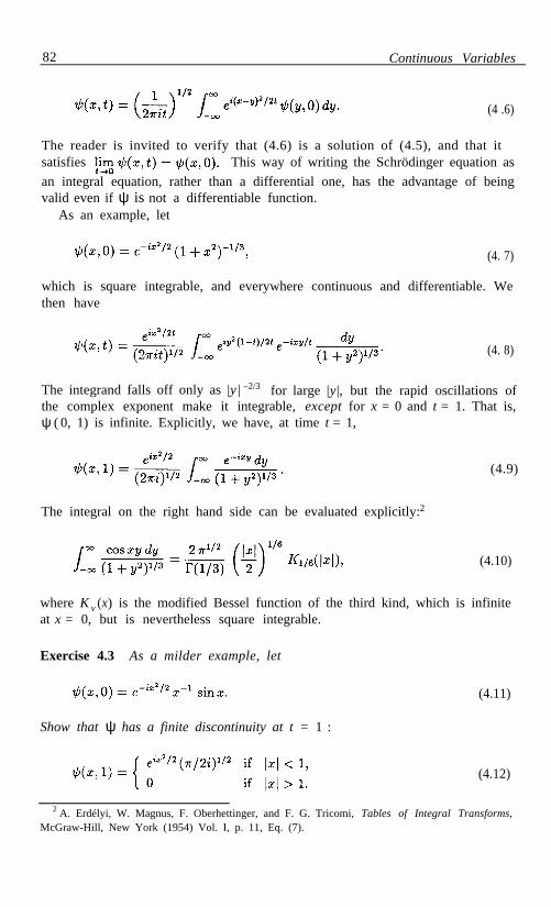
82 Continuous Variables
(4 .6)
The reader is invited to verify that (4.6) is a solution of (4.5), and that itsatisfies This way of writing the Schrödinger equation as
an integral equation, rather than a differential one, has the advantage of beingvalid even if ψ is not a differentiable function.
As an example, let
(4. 7)
which is square integrable, and everywhere continuous and differentiable. Wethen have
(4. 8)
The integrand falls off only as |y | –2/3 for large |y|, but the rapid oscillations ofthe complex exponent make it integrable, except for x = 0 and t = 1. That is,ψ ( 0, 1) is infinite. Explicitly, we have, at time t = 1,
(4.9)
The integral on the right hand side can be evaluated explicitly:2
(4.10)
where K v (x) is the modified Bessel function of the third kind, which is infiniteat x = 0, but is nevertheless square integrable.
Exercise 4.3 As a milder example, let
Show that ψ has a finite discontinuity at t = 1 :
(4.11)
(4.12)
2 A. Erdélyi, W. Magnus, F. Oberhettinger, and F. G. Tricomi, Tables of Integral Transforms,McGraw-Hill, New York (1954) Vol. I, p. 11, Eq. (7).

Hilbert space 83
Separability3
A Hilbert space is separable if there exists a countable set of vectors em suchthat any v ∈ H can be written as in Eq. (3.6),
(4.13)
with ⟨em , en ⟩ = δm n , and finite. This way of writing v as a discretesum does not preclude the possibility of representing it by means of a functionof a continuous variable, such as v (x). As a simple example of a relationshipbetween a discrete basis and a representation by continuous variables, let Hconsist of all the square integrable functions v(x) on the segment 0 ≤ x ≤ 2 π,with scalar product defined by
(4.14)
Dirichlet’s theorem asserts that any v (x) having at most a finite number ofmaxima, minima, and discontinuities, can be represented, except at isolatedpoints, by a Fourier series
(4.15)
where
(4.16)
That is, the function v(x) contains the same information as a countable set ofFourier coefficients. Note that
If you want a counterexample, a set of functions that do not satisfy Dirichlet’sconditions is These functions are everywhere continuousand differentiable, but they have infinitely many maxima and minima nearx = 0. Therefore, these ƒ (x) cannot be represented, as in Eq. (4.15), by acountable orthonormal basis, independent of the parameter a.
Nonseparable Hilbert spaces involve mathematical intricacies well beyond thescope of this book. I mentioned them because the quantization of fields (that is,of classical dynamical systems with a countable infinity of degrees of freedom)inexorably leads to nonseparable Hilbert spaces.4 It also leads to superselectionrules which restrict the validity of the superposition principle. Fortunately,ordinary quantum mechanics requires only a separable Hilbert space. It mayinvolve discontinuous wave functions, but not “pathological” ones.
3The word “separability” here has a meaning completely different from the “separability”that will be discussed in Chapter 6.
4G. Barton, Introduction to Advanced Field Theory (Interscience, New York, 1963),Chapt. 13.

84 Continuous Variables
4-2. Linear operators
Next, consider infinite dimensional matrices, which map vectors into vectors. Asbefore, I shall mention only the most important new features which result fromthe infinite dimensionality. It will be no surprise to encounter again convergenceproblems.
For example, the innocent looking matrix
(4.17)
gives, when we expand v = Au,
(4.18)
and
(4.19)
The expression Σ un which appears in (4.18)may diverge, even ifis finite (e.g., u n = 1/n). Therefore Au is not defined for every vector u .Moreover, even if Σ u n is finite, so that v1 in (4.18) has a meaning, v itself isnot an element of Hilbert space, because diverges (unless u1 = 0).
Exercise 4.4 Show that if A is defined as above, A2
does not exist.
These convergence problems lead to the notion of domain of definition of anoperator A: this is a set of elements u ∈ H, such that v = Au also is an elementof H. The domain of definition of an operator A can be the entire Hilbert spaceif, and only if, ||Au || is bounded, for any normalized u. The norm ||A|| of abounded linear operator is defined by
(4.20)
Exercise 4.5 Show that any unitary operator satisfies ||U|| = 1.
Exercise 4.6 Show that, for a bounded operator A, and normalized vectorsu and v,
and (4.21)
Local and quasilocal operators
When we use continuous indices, an expression such as v = Au becomes
(4.22)

Linear operators 85
The analog of a diagonal matrix, , becomes
(4.23)
where δ(x – y) is Dirac’s delta function, defined for any continuous ƒ by
(4.24)
Intuitively, a delta function δ(z) has an exceedingly high and narrow peak atz = 0, satisfying Actually, its structure may be much morecomplicated. These generalized functions, called distributions, are discussed inan appendix at the end of this chapter.
If Eq. (4.23) holds, Eq. (4.22) becomes v (x ) = a (x )u(x ). In that case, theoperator A is local, in the x basis: its meaning simply is multiplication by thefunction a(x). That function is called the x representation of A.
Likewise, one can define a quasilocal operator as the continuous analog of aband matrix Instead of (4.23), we have
(4.25)
Integration by parts then gives
(4.26)
This means that the x representation of the observable B is the differentialoperator b(x)d/dx. Higher derivatives of the delta function likewise correspondto higher order differential operators.
These operators are unbounded, even if they are restricted to act only oncontinuous and differentiable functions. For example, let H consist of all thesquare integrable functions v( x ), on the segment 0 ≤ x ≤ 2 π, with scalarproduct defined by (4.14). A convenient basis is the setEquations (4.15) and (4.16) show that this set is complete, if m runs over allthe integers from –∞ to ∞ . Now let A := –id/dx, so that A w m = m wm.Then is finite for every m. However the sequence isunbounded, and therefore the operator A is unbounded too.
As a further example, consider the function sin x, with–∞ < x < ∞ , which appeared in Exercise 4.3. This function is continuousand differentiable. Nevertheless, it does not belong to the domain of defini-tion of because its derivative is not square integrable. Therefore thefree particle Schrödinger equation (4.5) is, strictly speaking, meaningless in thiscase. However, the equivalent integral equation (4.6) causes no difficulty: Evenif H is unbounded, the unitary operator has unit norm, and its do-main of definition is the entire Hilbert space. This unitary evolution operatoris therefore more fundamental than the Hermitian operator H.

86 Continuous Variables
Further definitions
The product of a linear operator by a number c is defined by (cA)v = c (Av ) ;the sum A + B of two linear operators, by (A + B) v = Av + Bv; and theirproduct AB by (AB)v = A ( Bv). Note that c A, A + B, and AB, also are linearoperators. The domain of definition of cA is the same as that of A. The domainof definition of A + B is defined as the intersection of those of A and B. Thedomain of definition of AB consists of the vectors v for which the expression Bvis defined and belongs to the domain of A. It is sometimes possible to extendthese domains, in a natural way, beyond the minimal boundaries guaranteed bythe preceding definitions.
Obviously, ordinary numbers are a trivial case of bounded linear operators.Therefore I shall often make no distinction between the number 1 and the unitoperator The null operator O is defined by the property Ou = 0, for everyvector u. Some elementary lemmas, which will be useful in the sequel, are listedin the following exercises:
Exercise 4.7 If ⟨u, v ⟩ = 0 for every v, then u = 0. Hint: Let v = u.
Exercise 4.8 If ⟨ Au, v ⟩ = 0 for every u and v, it follows that A = O.
Exercise 4.9 Show that if ⟨ Av, v ⟩ = 0 for every v, then A = O.
Exercise 4.10 Show that if A is bounded,
Exercise 4.11 Show that, for any two bounded operators A and B,
and (4.27)
Adjoint operator
Let an operator A be defined over a dense set5 of vectors v in Hilbert space.The adjoint operator, A*, is then defined by the relation
(4.28)
This equation determines A* uniquely, if u also belongs to a dense set. Indeed,if (4.28) has two solutions, these satisfyand whenceit follows that (this is proved by extending the result of Exercise4.8 to dense sets). However, there is in general no guarantee that the domainof A* is dense (possibly, it may contain only the element 0).6
An operator satisfying A* = A is called self-adjoint. Note that the equalityA* = A implies that both operators have the same domain of definition. It is
5 A set of vectors is dense if every vector in H can be approximated arbitrarily well by someelement of that set.
6 F. Riesz and B. Sz.-Nagy, Functional Analysis, Ungar, New York (1955) pp. 300, 305.

Linear operators 87
not enough if they act in the same way on the common part of their domainsof definition. This requirement is essential, as the following example shows.
Consider again the Hilbert space consisting of square integrable functions onthe segment 0 ≤ x ≤ 2 π, with scalar product given by (4.14). An operatorA = –id/dx is defined over all the differentiable functions v (x). We shall seethat its adjoint A* is also written –id/dx, but A* has a smaller domain: Itis defined only over differentiable functions u (x ) which satisfy the boundarycondition u(0) = u (2π) = 0. Indeed, we have
(4.29)
(4.30)
and since v(0) and v(2π) are arbitrary, the above expression will vanish if, andonly if, the function u (x) satisfies u (0) = u (2π) = 0. Thus, in this example,the domain of A* (which acts on u ) is smaller than that of A (which acts on v ) .This is written as
A ⊃ A* or A* ⊂ A, (4.31)
and we say that A is an extension of A*, or that A* is a restriction of A. Notethat both operators coincide in the common part of their domain of definition.
Closure
An operator A, with domain D A , is called closed if every sequence vn ∈ DAhas a limit v which also belongs to DA , and moreover the sequence Avn has alimit, which is Av. Even if A is not closed, its adjoint A*, defined by Eq. (4.28),is always closed, because the scalar product is a continuous function of itsarguments. It can be proved6 that if A is closed and D A is dense in H, thedomain of A* is also dense in H, and moreover A** = A.
Symmetric operators and self-adjoint extensions
An operator satisfying ⟨ u, Bv⟩ = ⟨ Bu, v⟩ in a dense domain of H, is calledsymmetric (another way of saying that is B ⊆ B* ). For example, in Eq. (4.29),A* is symmetric, but A is not. In the physics literature, the term “Hermitian”is often indiscriminately used for either self-adjoint or symmetric.
Exercise 4.12 Prove that, if A, B, A + B, and AB, have dense domains,
and (4.32)
Also, prove that (αA)* = A*, for any complex number α.

88 Continuous Variables
It is sometimes possible to extend the domain of definition of a symmetricoperator, so as to make it self-adjoint. A symmetric operator may even havean infinity of different self-adjoint extensions. For example, let us define afamily of operators Aα = –id/dx, whose domains of definition consist of thedifferentiable functions v(x) which satisfy
(4.33)
with 0 ≤ α < 1. All these differential operators are written –id/dx a n d“look the same,” but actually they are quite different, because their domainsof definition are different (they do not even overlap). For each one of theseoperators, it follows from (4.29) that the adjoint operator is again –id/dx.Now, however, the domain of definition of is the same as that of Aα , becausethe right hand side of (4.30) vanishes if the boundary condition
(4.34)
holds, as well as Eq. (4.33). Therefore . These are self-adjointextensions of the symmetric operator A* which was defined in Eq. (4.29). Eachvalue of α generates a different extension, which represents a different physicalobservable. The difference is clearly seen in the spectra of the various Aα , givenby the eigenvalue equation Aα v = λv. The latter is, explicitly, –i dv/dx = λ v ,with the boundary condition (4.33). The solutions are wherem is an integer. Therefore the eigenvalues (that is, the observable values) ofAα are m + α , and they are different for each α .
Aharonov-Bohm effect
Differential operators like Aα can be given a simple physical interpretation.Consider an infinitely long and narrow solenoid,7 carrying a magnetic flux Φ .There is no magnetic field B outside the solenoid, but nevertheless there must bea magnetic vector potential A , whose line integral around the solenoid satisfies
A · d r = Φ. For example, if we take cylindrical coordinates r,θ, z, with thez axis along the solenoid, and if the gauge is appropriately chosen, the vectorA has only an azimuthal component Φ /2πr (note that the flux Φ is gaugeinvariant). A free particle of mass m and charge q, moving in the region outsidethe solenoid, is classically described by a Hamiltonian
(4.35)
The classical canonical transformation, can then completelyeliminate the flux term from (4.35), so that the solenoid does not influence themotion of charges outside it. This is the expected classical result, since there isno magnetic field outside the solenoid.
7 Y. Aharonov and D. Bohm, Phys. Rev. 115 (1959) 485.

Commutators and uncertainty relations 89
In quantum mechanics (where pθ becomes there is likewise aunitary transformation, similar to the above canonical transformation, whicheliminates Φ from Schrödinger’s equation. That transformation is
(4.36)
giving
(4.37)
The Schrödinger equation, when written in terms of , then looks exactly likethat of a free particle—the flux Φ nowhere appears in it—but, on the otherhand, the new wave function must satisfy a boundary condition
(4.38)
instead of simply ψ (2π) = ψ (0). It is the boundary condition which dependson the external parameter Φ, and gives it physical relevance. In a practicalproblem, such as a scattering experiment in the region encircling the solenoid,we can either work with ψ and the expressions on the left hand side of (4.37),or with , given by (4.36). In the later case, the presence of the solenoid istaken into account by the boundary condition (4.38), rather than by the waveequation itself. These two alternative ways of representing the physical situationare completely equivalent.
Radial momentum
Not every symmetric operator has a self-adjoint extension. For example, letpr = –id/dr be defined over differentiable and square integrable functions v(r),in the domain 0 ≤ r < ∞, with v (∞ ) = 0, and inner product
(4.39)
A calculation similar to Eq. (4.29) shows that pr is symmetric if its domain isrestricted by the boundary condition v(0) = 0. Then, the domain of neednot be restricted by u (0) = 0. It can be proved that no adjustment similar toEqs. (4.33) and (4.34)can make the domains of pr and coincide.
4-3. Commutators and uncertainty relations
The formal derivation of the quantum uncertainty relations provides instructiveexamples of the importance of correctly specifying the domains of definition ofunbounded operators. However, before we discuss these mathematical issues, itis desirable to clarify the physical meaning of these so-called “uncertainties.”

90 Continuous Variables
Classical measurement theory tacitly assumes that physical quantities haveobjective, albeit unknown, numerical values. Measurement errors are caused byimperfections of the experimental equipment, not to mention those of the ob-servers themselves. Thus, if we repeatedly measure the same physical quantity,such as the length or the weight of a macroscopic object, the resulting valuesare scattered around some average. The most common and naive approach todata analysis simply is to proclaim this average as the “best” value that wasobtained for the physical quantity.
In general, there are many independent sources of instrumental errors. Ifthese errors have finite first and second moments, the central limit theorem8
asserts that unbiased experimental values have a Gaussian distribution. A con-venient estimate of the uncertainty of a variable X is the standard deviation
divided by the square root of the number of experi-mental data. This uncertainty is usually listed, with a ± sign, after the “best”value, to indicate the expected accuracy of the latter. For example, the solarluminosity recorded for the year 1990 was L = (3.826 ± 0.008) × 1026 watts.
In quantum physics too, there are instrumental errors, which, if due to manyindependent causes, are Gaussian distributed. However, even if we could haveperfectly reliable instruments, the results of identical quantum tests, followingidentical preparations, would not, in general, be identical. For example, if anatomic beam of spin particles, polarized in the z direction, is sent through aStern-Gerlach magnet oriented along the x direction, the resulting distributionof the observed magnetic moments µx may appear as in Fig. 4.1.
Fig. 4.1. Simulated scatter plot of a Stern-Gerlach experiment (each clustercontains 200 impact points, produced by a random number generator).
A naive application of the “best value” formalism would then yield ⟨µ x ⟩ 0,and give no useful information on the intrinsic magnetic moment of the atomsstudied in the experiment. Moreover, the standard deviation from this “bestvalue,” namely , is not at all the result of instrumentalerrors. The correct interpretation of the data shown in Fig. 4.1 is that µ x cantake two values, µ or –µ . Each one of the two clusters of impact points must betreated separately. The distance between the centers of the two clusters is notdue to an instrumental deficiency, but is a genuine, unavoidable quantum effect.It is the spread of points within each cluster which is related to experimentalimperfections, such as a poor collimation of the atomic beam. The actual
8 W. Feller, An Introduction to Probability Theory and Its Applications, Wiley, New York(1968) Vol. I, p. 244.
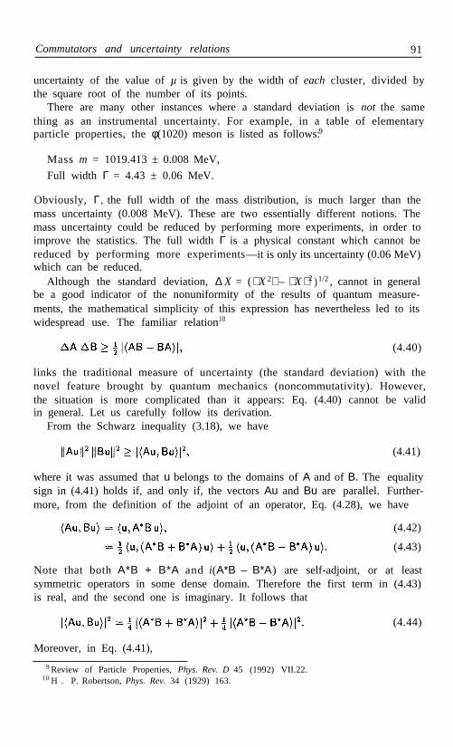
Commutators and uncertainty relations 91
uncertainty of the value of µ is given by the width of each cluster, divided bythe square root of the number of its points.
There are many other instances where a standard deviation is not the samething as an instrumental uncertainty. For example, in a table of elementaryparticle properties, the φ(1020) meson is listed as follows:9
Mass m = 1019.413 ± 0.008 MeV,
Full width Γ = 4.43 ± 0.06 MeV.
Obviously, Γ, the full width of the mass distribution, is much larger than themass uncertainty (0.008 MeV). These are two essentially different notions. Themass uncertainty could be reduced by performing more experiments, in order toimprove the statistics. The full width Γ is a physical constant which cannot bereduced by performing more experiments—it is only its uncertainty (0.06 MeV)which can be reduced.
Although the standard deviation, ∆ X = (⟨ X 2⟩ – ⟨ X ⟩ 2 )1/2, cannot in generalbe a good indicator of the nonuniformity of the results of quantum measure-ments, the mathematical simplicity of this expression has nevertheless led to itswidespread use. The familiar relation10
(4.40)
links the traditional measure of uncertainty (the standard deviation) with thenovel feature brought by quantum mechanics (noncommutativity). However,the situation is more complicated than it appears: Eq. (4.40) cannot be validin general. Let us carefully follow its derivation.
From the Schwarz inequality (3.18), we have
(4.41)
where it was assumed that u belongs to the domains of A and of B. The equalitysign in (4.41) holds if, and only if, the vectors Au and Bu are parallel. Further-more, from the definition of the adjoint of an operator, Eq. (4.28), we have
(4.42)
(4.43)
Note that both A*B + B*A and i(A*B – B*A) are self-adjoint, or at leastsymmetric operators in some dense domain. Therefore the first term in (4.43)is real, and the second one is imaginary. It follows that
(4.44)
Moreover, in Eq. (4.41),
9 Review of Particle Properties, Phys. Rev. D 45 (1992) VII.22.10H . P. Robertson, Phys. Rev. 34 (1929) 163.

92 Continuous Variables
(4.45)
(4.46)
(4.47)
Combining all these results, we obtain
Exercise 4.13 Show that
Hint: The expression behaves like a scalar product ⟨A, B⟩ , andin particular it satisfies a Schwarz inequality.11
*
In quantum theory, we are mostly interested in the case where A and B areself-adjoint operators, and (4.46) becomes
(4.48)
This equation remains valid if A is replaced by (A– a ), where a is any number,in particular a = ⟨ A⟩ . We then have
(4.49)
and likewise for ∆ B. The uncertainty relation (4.40) readily follows. Let usnow examine the conditions for attaining the equality sign in (4.40): the vectors(A – ⟨ A⟩ )u and (B– ⟨ B⟩ )u must be parallel and, moreover, the real contributionto (4.43) must vanish. The second requirement can be written as
(4.50)
It follows that, in the condition for parallelism,
(4.51)
the ratio α /ß is pure imaginary.Now, for all the foregoing mathematical manipulations to make sense, the
state vector u must belong not only to the domains of A and B , as in Eq. (4.41),but also to those of A * B, and B*A , and A*A , and B * B. Any vector u lyingoutside one of these domains (which may not even overlap!) may cause a vio-lation of the uncertainty relation (4.40).
Let us examine some examples. The simplest case is that of a Cartesian coor-dinate x and its conjugate momentum. In the x representation, these operatorsare x a n d respectively. Their commutator is
[ x, p] = (4.52)
11L. Pitaevskii and S. Stringari, J. Low Temp. Phys. 85 (1991) 377.

Commutators and uncertainty relations 93
Both operators are self-adjoint if the inner product of two vectors is
We then obtain the standard uncertainty relation
(4.53)
(4.54)
Now, since both x and p are unbounded operators, there are functions lyingoutside their domains of definition. For example, you may easily verify that thefunction (sin x
2
) /x , which is square integrable, belongs neither to the domainof x, nor to that of p. For such a function, both ∆ x and ∆ p are infinite, andEq. (4.54) is trivially satisfied—if it has any meaning.
Exercise 4.14 Show that the equality sign in (4.54) is attained only for
(4.55)
where a is real and positive, and b may be complex. Compute explicitly thenormalization constant C, and the values of ⟨x⟩ and ⟨ p⟩ for this “minimumuncertainty wave packet,” Hint: ψ must satisfy ( p – ⟨ p⟩)ψ = im ω( x – ⟨ x⟩ )ψ,where mω is a real constant with the dimensions of mass/time.
An uncertainty relation such as (4.54) is not a statement about the accuracyof our measuring instruments. On the contrary, its derivation assumes the exis-tence of perfect instruments (the experimental errors due to common laboratoryhardware are usually much larger than these quantum uncertainties). The onlycorrect interpretation of (4.54)is the following: If the same preparation proce-dure is repeated many times, and is followed either by a measurement of x, or bya measurement of p, the various results obtained for x and for p have standarddeviations, ∆ x and ∆ p, whose product cannot be less than/2. There neveris any question here that a measurement of x “disturbs” the value of p andvice-versa, as sometimes claimed. These measurements are indeed incompati-ble, but they are performed on different particles (all of which were identicallyprepared) and therefore these measurements cannot disturb each other in anyway. The uncertainty relation (4.54), or more generally (4.40), only reflects theintrinsic randomness of the outcomes of quantum tests.
Consider now an angular variable θ, with a range of values 0 ≤ θ ≤ 2π, andthe conjugate momentum . Both are self-adjoint operators if thescalar product is defined as in Eq. (4.14),and the domain of pθ is restrictedto differentiable functions which satisfy v(2π) = v (0). Shall we then have anuncertainty relation
(4.56)

94 Continuous Variables
This equation is obviously wrong. It is violated by all the eigenfunctions ofpθ , namely which trivially satisfy ∆pθ = 0, while their∆θ is about 1.8 (see next Exercise). It is not difficult to find the error. Theeigenfunctions um (θ) do not belong to the domain of the product pθ θ, because
does not satisfy the periodicity condition v(2π) = v (0), and thereforedoes not belong to the domain of pθ.
Exercise 4.15 Show that any eigenfunction of pθ gives
*
Exercise 4.16 Find three textbooks on quantum mechanics with the wronguncertainty relation (4.56), and one with the correct version.
Exercise 4.17 Find three other textbooks with the uncertainty relationRead carefully how each one of them explains the
meaning of this expression. This cannot be a special case of Eq. (4.40). Thetime t is not an operator (in classical mechanics, it is not a dynamical variable)so that ∆ t cannot be the standard deviation of the results of measurements oftime. (This issue is discussed in Sect. 12-8.) *
Case study: commutator of a product
From the well known identity,
[ A,BC ] ≡ [A,B ] C + B [A,C], (4.57)
one is tempted to infer that if A commutes with B and C, then A must alsocommute with the product BC. This conclusion is undoubtedly valid for finitematrices, but it may not be valid in an infinite dimensional Hilbert space, asthe following example shows.
Let H consist of square integrable functions of x, with a n dwith an inner product given by Eq. (4.53). Let the operators A, B, and C, begiven, in the x representation, as follows:
A = x / x ,
B = 1/x ,
C = x d/dx.
(4.58)
(4.59)
(4.60)
Then AB = BA = 1/ x , so that [A, B ] = 0. Likewise, AC = x d /dx a n d
(4.61)
The first term on the right hand side contains the derivative of the discontinuousfunction x / x |, which is 2δ(x ). It is apparently permissible to ignore this term,because xδ(x) is equal to zero when it multiplies a function ψ(x ) which is finiteat x = 0, or even a function which is infinite at the origin, as long as it is

Truncated Hilbert space 95
less singular than x – 1, for example, Now, any ψ (x) which issquare integrable must be less singular than x–1/2. Therefore, we can safelywrite AC = CA, when these operators act on functions belonging to H.
Consider now the product BC = d /dx. We have
[ A, BC] = [ x / x , d /dx ] = –2δ(x ), (4.62)
and this commutator for sure does not vanish, although A commutes with Band with C separately! Where is the error? A careful check of the foregoingcalculations shows that [A, C] = –2xδ(x ) ≠ 0 was set equal to zero, becausex δ(x ) = 0 whenever this expression is multiplied by a function belonging to H.But the operator B = 1/x, when acting on that function, makes it singular atthe origin, and then the resulting product B[A, C] = –2δ(x ) does not vanish.
This example shows the importance of being extremely careful with the do-mains of definition of unbounded operators. You will find more surprises in theexercises below.
Exercise 4.18 The scaling operator D(s ) is defined by
(4.63)
where s is a positive constant. Show that D ( s) is a unitary operator, and thatit commutes with the sign operator A defined by (4.58). Show moreover that[A, BD(s)] = 0, where B is defined by (4.59). *
From the scaling operator D(s ), defined above, one can obtainExercise 4.19a new operator,
(4.64)
Show that D' (1) = 1 + 2x d/dx = 1 + 2C, where C is the operator defined by(4.60). Thus, although A commutes with BD (s ) for all s, it does not commutewith the derivative BD' (1). *
4-4. Truncated Hilbert space
In the preceding chapter, we saw that physical observables are represented byHermitian matrices, according to the following prescription: The eigenvectorsof a matrix A form an orthonormal basis, whose elements correspond to thepure states defined by all the possible outcomes of a maximal quantum test;each one of these outcomes corresponds to one of the eigenvalues of A; thateigenvalue is then said to be the result of a measurement of A, by means of theaforementioned quantum test.
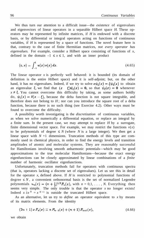
96 Continuous Variables
We thus turn our attention to a difficult issue—the existence of eigenvaluesand eigenvectors of linear operators in a separable Hilbert space H. These op-erators may be represented by infinite matrices, if H is endowed with a discretebasis, or by differential or integral operators acting on functions of continuousvariables, if H is represented by a space of functions. The novel feature here isthat, contrary to the case of finite Hermitian matrices, not every operator haseigenvalues. For example, consider a Hilbert space consisting of functions of x,defined in the domain –1 ≤ x ≤ 1, and with an inner product
(4.65)
The linear operator x is perfectly well behaved: it is bounded (its domain ofdefinition is the entire Hilbert space) and it is self-adjoint; but, on the otherhand, it has no eigenvalues. Indeed, if we try to solve to obtainan eigenvalue ξ, we find that so that wheneverx ≠ ξ. You cannot overcome this difficulty by taking, as some authors boldlydo, because the delta function is not square integrable, andtherefore does not belong to H ; nor can you introduce the square root of a deltafunction, because there is no such thing (see Exercise 4.2). Other ways must befound to overcome the difficulty.
A possibility worth investigating is the discretization of continuous variables,as when we solve numerically a differential equation, or replace an integral bya finite sum. In the present case, we may attempt to replace H by a surrogate,finite dimensional vector space. For example, we may restrict the functions v(x)to be polynomials of degree ≤ N (where N is a large integer). We then get alinear space with N +1 dimensions. Truncation methods of this type are com-monly used in chemical physics, in order to find the energy levels and transitionamplitudes of atomic and molecular systems. They are reasonably successfulfor Hamiltonians involving smooth anharmonic potentials—which may be goodapproximations to the true molecular Hamiltonians—because the exact energyeigenfunctions can be closely approximated by linear combinations of a finitenumber of harmonic oscillator eigenfunctions.
Unfortunately, truncation methods fail for operators with continuous spectra(that is, operators lacking a discrete set of eigenvalues). Let us see this in detailfor the operator x, defined above. If H is restricted to polynomial functions ofdegree ≤ N , a convenient orthonormal basis is the set of normalized Legendrepolynomials with n = 0,1, . . . , N. Everything thenseems very simple.The only trouble is that the operator x no longer exists!Indeed x Ž x N = x N +1 is outside the truncated Hilbert space.
As an alternative, let us try to define an operator equivalent to x by meansof its matrix elements. From the identity
(4.66)
we obtain

Truncated Hilbert space 97
(4.67)
(4.68)
(4.69)
whence
This matrix correctly represents the operator x if the indices m and n canrun to infinity. Here however, the matrix is truncated for m or n ≥ N. It isthis truncation which causes it to have properties different from those of theoriginal operator x. How badly different is it? This can be seen by inspectingthe eigenvalues and the eigenfunctions of the operator represented by the bandmatrix x mn . We first have to solve
(4.70)
to find the N + 1 eigenvalues ξ and the corresponding eigenvectors (this iseasily done numerically, since xmn already is in tridiagonal form). Then, foreach ξ, we may obtain the x representation of the eigenvector vn—that is, theeigenfunction v (x )—by
(4.71)
The result is shown in Fig. 4.2, for N = 100. First, we notice that theeigenvalues are not evenly distributed between –1 and 1. They are more con-centrated toward the extremities. We also see that a typical eigenfunction (the60th, in this case) has, as intuitively expected, a sharp peak at the correspond-ing eigenvalue. But it also has fringes all over the domain of x. These fringes arenecessary in order to ensure its orthogonality to the other eigenfunctions. Notein particular the overshoot (Gibbs phenomenon) at x = ±1. These propertiesare not unexpected. They resemble those of the delta functions which will bediscussed in an appendix to this chapter (see Fig. 4.4).
As a further exercise, let us examine the matrix elements of the operatorp = – i d/dx. They are
(4.72)
where as before. Integration by parts gives
(4.73)

98 Continuous Variables
because P m(±1) = (±1)m . The parity and orthogonality properties of Legendrepolynomials ensure that the integral on the left hand side vanishes, unless n =m + 1, m + 3,...; and in that case, it is the integral on the right hand side
(4.74)
that must vanish. We therefore obtain
Fig. 4.2. The 101 eigenvalues of the truncated operator x are shown by thebars at the top of the figure. The normalized eigenfunction correspondingto the 60th eigenvalue (which is 0.27497 27848) has a sharp peak there, butis also spread throughout the entire domain of x, from –1 to 1.
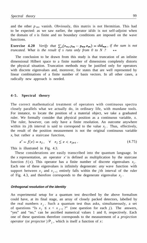
Spectral theory 99
and the other p mn vanish. Obviously, this matrix is not Hermitian. This hadto be expected: as we saw earlier, the operator id/dx is not self-adjoint whenthe domain of x is finite and no boundary conditions are imposed on the wavefunctions.
Exercise 4.20 Verify that if the sum is nottruncated. What is the result if s runs only from 0 to N ? **
The conclusion to be drawn from this study is that truncation of an infinitedimensional Hilbert space to a finite number of dimensions completely distortsthe physical situation. Truncation methods may be justified only for operatorswith discrete eigenvalues and, moreover, for states that are well represented bylinear combinations of a finite number of basis vectors. In all other cases, aradically new approach is needed.
4-5 . Spectral theory
The correct mathematical treatment of operators with continuous spectraclosely parallels what we actually do, in ordinary life, with mundane tools.For instance, to locate the position of a material object, we take a graduatedruler. We formally consider that physical position as a continuous variable, x.The ruler, however, can only have a finite resolution. An outcome anywherewithin its j th interval is said to correspond to the value xj . Thus, effectively,the result of the position measurement is not the original continuous variablex, but rather a staircase function,
(4.75)
This is illustrated in Fig. 4.3.These considerations are easily transcribed into the quantum language. In
the x representation, an operator x' is defined as multiplication by the staircasefunction ƒ ( x). This operator has a finite number of discrete eigenvalues xj .Each one of these eigenvalues is infinitely degenerate: any wave function withsupport between x j and x j +1 entirely falls within the j th interval of the rulerof Fig. 4.3, and therefore corresponds to the degenerate eigenvalue xj .
Orthogonal resolution of the identity
An experimental setup for a quantum test described by the above formalismcould have, at its final stage, an array of closely packed detectors, labelled bythe real numbers x j . Such a quantum test thus asks, simultaneously, a setof questions “Is x j ≤ x < x j +1 ?” (one question for each j ). The answers,“yes” and “no,” can be ascribed numerical values 1 and 0, respectively. Eachone of these questions therefore corresponds to the measurement of a projectionoperator (or projector ) P j , which is itself a function of x :

100 Continuous Variables
Fig. 4.3. (a) The magnifying glass shows the details of a rulerused to measure the continuous observable x. (b) The resultof the measurement is given by the staircase function ƒ(x ).
if x j ≤ x < x j +1 ,otherwise.
(4.76)
(4.77)
(4.78)
These projectors obviously satisfy
P j Pk = δjk Pk ,
and
The staircase operator x' = ƒ( x ), defined by Eq. (4.75), can then be written as
(4.79)
(4.80)
It satisfies

Spectral theory 101
so that the operator x' indeed approximates the operator x, as well as allowedby the finite resolution of the ruler in Fig. 4.3.
Exercise 4.21 Prove Eq. (4.80).
How do we proceed to the continuum limit? We could rely on Eq. (4.80),and imagine that we have an infinite sequence of rulers, divided in centimeters,millimeters, and so on, getting arbitrarily close to the abstract notion of acontinuous length. However, it is more efficient to proceed as follows.
Let us define a spectral family of operators
(4.81)
They obey the recursion relation
E( x j +1 ) = E(x j ) + P j , (4.82)
and the boundary conditions
E( xmin ) = O
) is the question “Is x < x ?” withj
answers yes = 1, and no = 0. As can be seen from Eq. (4.77), these E (xj ) areprojectors. They act like a sequence of sieves, satisfying
It is now easy to pass to the continuum limit: We define E(ξ
ξ and ξ +dξ, and define an “infinitesimal” projector,
which represents the question “Is ξ ≤ x < ξ + d ξ ?”. This d E(ξ
staircase approximation (4.79), the exact result
Note that the integration limits actually are operators, namely E(x min
and E (xmax) = , in accordance with (4.83).
of the operator x, and the operators E(ξ
the operator x in a way analogous to Eq. (3.58):
E( xmax) = . (4.83)
The physical meaning of the operator E(x j
(4.84)
) as the projectorwhich represents the question “Is x < ξ ?” and which returns, as the answer, anumerical value (yes = 1, no = 0). We can then consider two neighboring values,
(4.85)
) thus behavesas an infinitesimal increment Pj in Eq. (4.82). We then have, instead of the
(4.86)
) = O,
Equation (4.86) is called the spectral decomposition, or spectral resolution,) are the spectral family (also called
resolution of the identity) generated by x. We can now define any function of
and

102 Continuous Variables
(4.87)
The right hand sides of Eqs. (4.86) and (4.87) are called Stieltjes integrals.Consider now a small increment dξ → 0. If the limit d E( ξ) /d ξ exists, the
integration step can be taken as the c-number dξ, rather than d E(ξ ), which isan operator. We then have an operator valued Riemann integral:
(4.88)
It can be shown12 that any self-adjoint operator generates a unique resolutionof the identity. A spectral decomposition such as (4.86) applies not only tooperators with continuous spectra, but also to those having discrete spectra, oreven mixed ones, like the Hamiltonian of the hydrogen atom. For a discretespectrum, dE(ξ) = 0 if ξ lies between consecutive eigenvalues, and dE(ξ ) = Pk,namely the projector on the kth eigenstate, if the kth eigenvalue lies between ξand ξ + d ξ .
Note that in any case the projector E(ξ ) is a bounded operator, which dependson the parameter ξ . It may be a discontinuous function of ξ, but it never isinfinite, and we never actually need d E(ξ) /dξ. This is the advantage of theStieltjes integral over the more familiar Riemann integral: the left hand side of(4.88) is always meaningful, even if the right hand side is not.
Exercise 4.22 Show that, if ƒ(ξ ) is a real function, then ƒ( x), defined byEq. (4.87), is a self-adjoint operator.
Exercise 4.23 Show that two operators that have the same spectral familyare functions of each other.
Exercise 4.24 Show, directly from Eq. (4.84), that, for a given spectral familyE( λ ),
(4.89)
This is an important property, which will be used later.
Exercise 4.25 Show that, if ƒ(ξ)the spectral representation (4.86), the expression
is a unitary operator. Hint: Use the results of the preceding exercises.
1 2
p. 176.
is a real function, and x is an operator with
(4.90)
M. H. Stone, Linear Transformations in Hilbert Space, Amer. Math. Soc., New York (1932)

Classification of spectra 103
The spectral decomposition of self-adjoint operators allows one to give arigorous definition of the measurement of a continuous variable. The latter isequivalent to an infinite set of yes-no questions. Each question is represented bya bounded (but infinitely degenerate) projection operator. However, this formalapproach is unable to give a meaning to the measurement of operators that arenot self-adjoint, such as the radial momentum – i d / dr (with 0 ≤ r < ∞ )whose properties were discussed on page 89. Yet, in classical mechanics, pr is awell defined variable. It thus appears that there can be no strict correspondencebetween classical mechanics and quantum theory.
4-6. Classification of spectra
Self-adjoint operators may have a discrete spectrum—with well separated eigen-values and with a complete set of normalizable eigenvectors—or a continuousspectrum, or a mixed one. A mixed spectrum may have a finite number ofdiscrete eigenvalues, or even a denumerable infinity of them; typical examplesare the bound energy levels of a finite potential well, and those of the hydro-gen atom, respectively. In both cases, there is, above the discrete spectrum, acontinuous spectrum of unbound states.
Although an operator A with a continuous spectrum has, strictly speaking,no eigenvectors at all, each point λ of that spectrum (that is, each point wheredE( ξ) / dξ exists and is not O ) is “almost an eigenvalue” in the following sense:It is possible to construct states ψλ satisfying
(4.91)
with arbitrarily small positive ∈. Indeed, let E(ξ ) be the spectral family of A.Define a projector
(4.92)
and let ψλ be any eigenstate of Pλ with eigenvalue 1, that is to say,
(4.93)
Such a ψλ is easily constructed by taking any state φ for which P λ φ ≠ 0. Thenormalized vector will then satisfy (4.93). For example, ifA = x, the x -representation of ψλ is any function ψ (x ) with support betweenλ – ∈ and λ + ∈ .
To prove (4.91), we note that, by virtue of (4.89),
(4.94)

104 Continuous Variables
and we thus have
(4.95)
(4.96)
where (4.89) was used again. The last expression can be transformed into anordinary integral (that is, into a sum of c-numbers):
(4.97)
The integral on the right hand side simply isThis completes the proof of Eq. (4.91).
More generally, we have
If the function ƒ can be expanded into a Taylor series around λ ,
(4.99)
the right hand side of (4.98) becomes
(4.100)
Therefore, states ψλ can be constructed in such a way that, for any smoothfunction ƒ, the mean value ⟨ ƒ(A) ⟩ is arbitrarily close to ƒ(λ ). This is in sharpcontrast to the situation prevailing in the empty regions between eigenvalues ofa discrete spectrum: While it is easy to construct superpositions of eigenstatesof an operator A such that, on the average, (for any real µ betweentwo discrete eigenvalues), the variance
cannot be made arbitrarily small.
Exercise 4.26 Let λ m and λ n
let v m and vn be the corresponding eigenvectors. LetShow that θ can be chosen in such a way thatvalue between λm and λn . What is then the variance
(4.98)
(4.101)
be consecutive discrete eigenvalues of A, and
will take any desired

Classification of spectra 105
Bound states embedded in a continuum
The discrete and continuous parts of a mixed spectrum are not always disjoint.They may also overlap: discrete eigenvalues, which correspond to normalizableeigenvectors, may be embedded in a continuous spectrum (that is, the intervalsbetween these discrete eigenvalues are not empty). For example, consider twohydrogen atoms, far away from each other. Their mutual interaction is negligi-ble. If we also neglect their interaction with the quantized electromagnetic fieldvacuum, each atom has an infinite number of stable energy levels. The lowestones are E 1 = –13.6eV and E 2 = –3.4eV. Each atom also has a continuousspectrum, E ≥ 0. Therefore the two atoms together have, among their discreteeigenvalues, one at 2E 2 = –6.8eV, which is higher than the threshold of theircontinuous spectrum, namely E ≥ E 1 .
However, if we take into account the mutual interaction of the two atoms,this discrete eigenvalue (with both atoms in an excited n = 2 state) becomesmetastable: it actually is a resonance. The system will eventually undergoan autoionization transition, whereby one of the electrons falls into its n = 1ground state, and the other electron escapes to infinity.
Exercise 4.27 Estimate the mean decay time by autoionization of this H2system, as a function of the distance between the atoms.
A similar situation occurs in the Auger effect. An atom can be excited insuch a way that an electron from the innermost shell is transferred into a higher,incomplete shell. The result is an eigenstate of the Hamiltonian of the atom,13
with all the electrons bound. However, the total energy of that excited atomis compatible with other electronic configurations, where the innermost shell isoccupied and one of the electrons is free. The resulting positive ion has, like theneutral atom, discrete energy levels; but, on the other hand, the kinetic energyof the free electron has a continuous spectrum. In this way, discrete energylevels of the neutral atom are embedded in the continuous spectrum of the ion-electron system. Here too, most of these “discrete energy levels” actually arevery narrow and long lived resonances, which decay by autoionization. It is onlythe use of an approximate Hamiltonian, where some interactions are neglected,which make these levels appear discrete and stable.
Still another type of spectrum, which at first sight may seem rather bizarre,but which will actually appear in a future application (Sect. 10-5), consists ofa dense set of discrete eigenvalues. As a simple example, consider the Hilbertspace of functions ψ( x , y ), with 0 ≤ x , y < 2π. The scalar product is given by
13The Auger effect is a nonradiative rearrangement of the electrons. In the present discussion,the atomic nucleus is assumed fixed, and the Hamiltonian does not include any interaction withthe quantized electromagnetic field.
(4.102)

106 Continuous Variables
In that space let an operator,
be defined over the subset of differentiable functions ψ (x, y ) which satisfy theboundary conditions
ψ (2π, y ) = ψ (0, y)
That operator is self-adjoint. Its normalized eigenfunctions are ei( mx+ny ) /2π,corresponding to eigenvalues m + n, with m and n running over positiveand negative integers.
This spectrum looks very simple, but its physical implications are curious.Suppose that a measurement of A yields the result α , with an expected accuracy± ∈ . (The estimated error ±∈ is solely due to the finite instrumental resolution,it is not a quantum effect.) What can now be said about the correspondingeigenstates (that is, the corresponding quantum numbers m and n) ? The latterare obtained from the equation
which has, for arbitrarily small positive ∈ , an infinity of solutions m and n .This is intuitively seen by noting that (4.105) represents a narrow strip in
the mn plane. That strip, which has an irrational slope, contains an infinity ofpoints with integral coordinates m and n. The smaller ∈ , the larger the averagedistance between consecutive values of m and n. While an exact measurementof A (for example, α = 7 – 5 , exactly) would yield unambiguous values form and n, and therefore well defined eigenstates of the commuting operators–id/dx and –id/dy, the least inaccuracy ∈ leaves us with an infinite set ofwidely different m, n pairs.
Finally, one more type of pathological spectrum is worth mentioning: It isa singular continuous spectum, whose support is a Cantor set—an uncountableset which may, but need not, have zero Lebesgue measure. Spectra of this kindmay occur for Hamiltonians with an almost periodic potential.14
4-7. Appendix: Generalized functions
The use of singular δ −functions, originally introduced by Dirac, was criticizedby von Neumann, in the preface of his book:15
14 J. Avron and B. Simon, Bull. Am. Math. Soc. 6 (1982) 81.15 J. von Neumann, Mathematische Grundlagen der Quantenmechanik, Springer, Berlin
(1932); transl.: Mathematical Foundations of Quantum Mechanics, Princeton Univ. Press,Princeton (1955).
(4.103)
ψ ( x,2π) = ψ (x ,0). (4.104)
(4.105)
and

Appendix: Generalized functions 107
The method of Dirac, mentioned above, (and this is overlooked today ina great part of quantum mechanical literature, because of the clarity andelegance of the theory) in no way satisfies the requirements of mathematicalrigor—not even if these are reduced in a natural and proper fashion tothe extent common elsewhere in theoretical physics. For example, themethod adheres to the fiction that each self-adjoint operator can be put indiagonal form. In the case of those operators for which this is not actuallythe case, this requires the introduction of “improper” functions with self-contradictory properties. The insertion of such a mathematical “fiction”is frequently necessary in Dirac’s approach, even though the problem athand is merely one of calculating numerically the result of a clearly definedexperiment. There would be no objection here if these concepts, whichcannot be incorporated into the present day framework of analysis, wereintrinsically necessary for the physical theory . . . . But this is by no meansthe case . . . . It should be emphasized that the correct structure need notconsist in a mathematical refinement and explanation of the Dirac method,but rather that it requires a procedure differing from the very beginning,namely, the reliance on the Hilbert theory of operators.
In this chapter, I followed von Neumann’s approach, to give some idea ofits flavor. I did not attempt to be mathematically rigorous nor complete; moreinformation can be found in the treatises listed in the bibliography. The purposeof the present appendix is to partly rehabilitate Dirac’s delta functions, and toclarify the conditions under which their use is legitimate.
From the pure mathematician’s point of view, a space whose elements areordinary functions with regular properties may be embedded in a larger space,whose elements are of a more abstract character. In this larger space, theoperations of analysis may be carried out more freely, and the theorems takeon a simpler and more elegant form. For example, the theory of distributions,developed by Schwartz,16 is a rigorous version of Dirac’s intuitive delta functionformalism.
These distributions can often be obtained as improper limits, that I shalldenote by writing “lim” between quotation marks. However, as we shallsee, their properties are quite different from those sketched in Dirac’s graphicdescription:17
To get a picture of δ(x), take a function of the real variable x which vanisheseverywhere except inside a small domain, of length ∈ say, surrounding theorigin x = 0, and which is so large inside this domain that its integral overthis domain is unity. The exact shape of the function inside this domaindoes not matter, provided that there are no unnecessarily wild variations(for example, provided that the function is always of order ∈ – 1). Then inthe limit ∈ → 0 this function will go over into δ (x).
16 L. Schwartz, Théorie des Distributions, Hermann, Paris (1950).17P. A. M. Dirac, The Principles of Quantum Mechanics, Oxford Univ. Press (1947), p. 58.

108 Continuous Variables
A simple example will show that things are different from Dirac’s intuitivepicture. From the properties of Fourier series, Eqs. (4.15) and (4.16), we have
Let us boldly exchange the order of summation. We obtain
whence we infer
To give a meaning to this infinite sum—when it stands alone, rather than insidean integral as in (4.107)—let us try to consider it as the “limit” of a finite sum,from – M to M, when M → ∞.which is easily evaluated, with result
to have a sharp peak of height M / πnearest zeros occur at z = ± π/ M. Thus, the area of the peak is roughly unity.However, the function (4.109) does not vanish outside that narrow domain.Rather, it rapidly oscillates, with a period 2πamplitude, which is about 1/πz for |z|oscillations, we have, for any smooth function ƒ,
property of delta functions:
in the vicinity of x.
polynomials, in the domain –1 ≤ x ≤ 1. Formally, we have
(4.106)
(4.107)
(4.108)
This finite sum is a geometric progression
(4.109)
where z denotes x—y, for brevity. For large M, the right hand side is easily seenat z = 0. On each side of the peak, the
/ M, and with a slowly decreasing1. As a consequence of these rapid
(4.110)
This approximation is valid for large M, and for functions ƒ whose variation ismuch slower than that of the first factor in the integrand of (4.110). Under theseconditions, the “limit” of Eq. (4.109) for M → ∞ satisfies the fundamental
(4.111)
Note that this result is valid only for functions ƒ that are sufficiently smooth
Another example of delta function, showing a different morphology, can beobtained by using the orthogonality and completeness properties of Legendre

Appendix: Generalized functions 109
(4.112)
because, if we multiply this equation by Pn (y ) and integrate over y, both sidesgive the same result, namely Pn (x ). As the Legendre polynomials form a com-plete basis, the same property will hold for any “reasonable” function whichcan be expanded into a sum of Pn (x ). Let us however examine how the “limit”m → ∞ is attained. We have, from the Christoffel-Darboux formula,18
Figure 4.4 show a plot of this expression, as a function of x, for n = 100 andy = . There is a striking resemblance with Fig. 4.2; even the overshoot (Gibbsphenomenon) at x = ±1 looks the same. However, the vertical scales in thesefigures are completely different. The area under the curve in Fig. 4.4 is equalto 1 (see next Exercise). On the other hand, Fig. 4.2 represents a normalizedeigenfunction V (x ) of the truncated operator x, given by Eq. (4.71), and it isthe integral of |v (x )|² which is equal to 1.
Exercise 4.28 Show that if the left hand side of (4.113) is multiplied by xk ,for any k ≤ n, and then integrated over x, the result is y k .
Exercise 4.29 Use the asymptotic expansion of Pn (x ) for large n to obtain asimple estimate of the right hand side of (4.113).
Exercise 4.30 Show that
where P denotes the principal value. Hint: Consider the real and imaginaryparts of this equation.
We thus see that delta functions (or tempered distributions, as they are calledin the mathematical literature) can be given rigorous definitions, and are alegitimate computational tool. However, these are not functions, in the usualsense of this word, and one must be careful not to misuse them. In particular,they cannot represent quantum states, because they are not square integrable,and therefore not members of a Hilbert space; nor can we consistently definethe square root of a delta function, as we attempted to do in Exercise 4.2.
An essential property of delta functions is that they can safely be used onlywhen they appear in expressions in which they are multiplied by other, smooth
18I. S. Gradshteyn and I. M. Ryzhik, Table of Integrals, Series, and Products, AcademicPress, New York (1980) p. 1026.
(4.113)
(4.114)

110 Continuous Variables
Fig. 4.4. A truncated delta function: The expression in Eq. (4.113)is plotted as a function of x, for y = and n = 100.
functions. Only then is the meaning of these expressions unambiguous. In anyother case, the result is ill defined.
Quantum fields
However, these other cases do occur—they even play a central role in quantumfield theory. The latter is an extension of quantum mechanics, in which thedynamical variables are fields, such as E (r, t ) or B (r , t ). Here, the symbol rdoes not represent a dynamical variable; rather, it serves as a continuous indexfor the set of variables, E and B. We thus have an infinite number of degrees
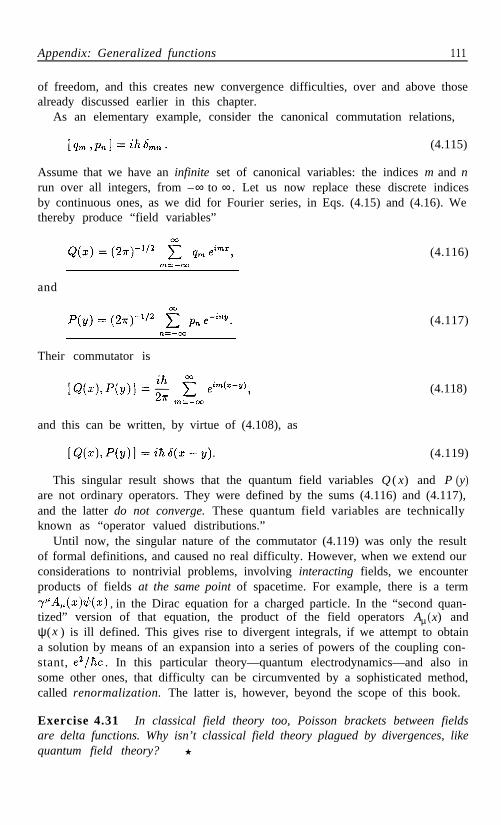
Appendix: Generalized functions 111
of freedom, and this creates new convergence difficulties, over and above thosealready discussed earlier in this chapter.
As an elementary example, consider the canonical commutation relations,
(4.115)
Assume that we have an infinite set of canonical variables: the indices m and nrun over all integers, from –∞ to ∞ . Let us now replace these discrete indicesby continuous ones, as we did for Fourier series, in Eqs. (4.15) and (4.16). Wethereby produce “field variables”
and
Their commutator is
(4.116)
(4.117)
(4.118)
(4.119)
and this can be written, by virtue of (4.108), as
This singular result shows that the quantum field variables Q ( x) and P (y)are not ordinary operators. They were defined by the sums (4.116) and (4.117),and the latter do not converge. These quantum field variables are technicallyknown as “operator valued distributions.”
Until now, the singular nature of the commutator (4.119) was only the resultof formal definitions, and caused no real difficulty. However, when we extend ourconsiderations to nontrivial problems, involving interacting fields, we encounterproducts of fields at the same point of spacetime. For example, there is a term
, in the Dirac equation for a charged particle. In the “second quan-tized” version of that equation, the product of the field operators Aµ (x) andψ(x ) is ill defined. This gives rise to divergent integrals, if we attempt to obtaina solution by means of an expansion into a series of powers of the coupling con-stant, . In this particular theory—quantum electrodynamics—and also insome other ones, that difficulty can be circumvented by a sophisticated method,called renormalization. The latter is, however, beyond the scope of this book.
Exercise 4.31 In classical field theory too, Poisson brackets between fieldsare delta functions. Why isn’t classical field theory plagued by divergences, likequantum field theory?

112 Continuous Variables
4-8. Bibliography
The purpose of this chapter was to highlight some mathematical aspects ofquantum theory, which are usually ignored in introductory texts. Only a fewselected topics were treated. More complete discussions can be found in thefollowing sources:
T. F. Jordan, Linear Operators for Quantum Mechanics, Wiley, New York(1969) [reprinted by Krieger].
This book was specifically written to be a companion to quantum mechanics texts.Its compact presentation clearly shows the logic and simplicity of the mathematicalstructure of quantum theory. Rigorous proofs are supplied, if they are reasonablyshort. Long and difficult proofs are replaced by references to more complete treatises,such as
F. Riesz and B. Sz.-Nagy, Functional Analysis, Ungar, New York (1955)[reprinted by Dover].
P. Roman, Some Modern Mathematics for Physicists and Other Outsiders,Pergamon, New York (1975). Vol. I: Algebra, topology, and measure theory;Vol. II: Functional analysis with applications.
The author, whose previous publications include well known textbooks on particlephysics and quantum theory, writes in the preface: “. . . this book may fill the needsof most theoretical physicists (especially of those interested in quantum theory, highenergy physics, relativity, modern statistical physics) . . . However, this is a book onmathematics and the student who patiently made his way through it will be ableto understand any contemporary mathematical source that is needed to enlarge theknowledge gained from this volume.”
M. Reed and B. Simon, Methods of Modern Mathematical Physics, AcademicPress, New York. Vol. I: Functional analysis (1980); Vol. II: Fourier analysis,self-adjointness (1975); Vol. III: Scattering theory (1979); Vol. IV: Analysis ofoperators (1978).
This four volume encyclopedia covers nearly every aspect of mathematics that maybe needed by a quantum theorist.
Mathematical paradoxes
C. Zhu and J. R. Klauder, “Classical symptoms of quantum illnesses,” Am.J. Phys. 61 (1993) 605.
O. E. Alon, N. Moiseyev and A. Peres, “Infinite matrices may violate theassociative law,” J. Phys. A 28 (1995) 1765.

Part II
CRYPTODETERMINISM
AND QUANTUM
INSEPARABILITY

Plate II. The Kochen-Specker theorem, discussed in Chapter 7, is of funda-mental importance for quantum theory. Its most “economical” proof makesuse of 31 rays, which form 17 orthogonal triads (see Exercise 7.20, page 211).These rays are obtained by connecting the center of the cube to the black dotson its faces and edges (the six gray dots are not used in that proof). Thisconstruction should be compared with the cube in Fig. 7.2, on page 198.
114

Chapter 5
Composite Systems
5-1. Quantum correlations
A composite system is one that includes several quantum objects (for example,a hydrogen atom consists of a proton and an electron). Our problem is toconstruct a formalism whereby the state of a composite system is expressed interms of states of its constituents.
The situation is simple if the electron and the proton are widely separated—they may possibly be in different laboratories, where they have been preparedin states u and v, respectively. (This is not, of course, what is commonly calleda hydrogen atom.) The vectors u and v belong to different Hilbert spaces. Itis possible to represent them by functions u (re ) and v (rp ), where r e and rp
are Cartesian coordinates used to describe the states of the electron and theproton, respectively. However, in order to make our first acquaintance withthis problem, it is preferable to use a discrete basis, where the components ofu and v are um and vv , with the Hilbert space of electron states labelled byLatin indices, and that of proton states by Greek indices.¹ The state of bothparticles together can then be represented as a direct product (sometimes called“tensor product”) of these two vectors, written as w = u ⊗ v. The componentsof w are w mv = u mvv . In that expression, one must consider mv as a singlevector index, whose values can conveniently be listed in alphabetical order:
and so on.Direct products can represent the state of two (or more) systems that have
been prepared independently. However, the main issue that we want to in-vestigate is the description of interacting particles—for example, of a genuinehydrogen atom. Let us tentatively assume that composite systems do not differin any essential way from “elementary” ones, and in particular that they obeythe principle of superposition G (see page 50). Namely, if u1 and u 2 are possiblestates of an electron, and v 1 and v2 possible states of a proton, the expression
is a realizable state of an electron-proton system.
¹ Here, indices taken from different alphabets are used to label different vector spaces. Inpreceding chapters, they denoted different bases in the same vector space.
115

116 Composite Systems
Note that, in this combined state w, neither the electron nor the proton is ina pure quantum state: There is no complete test for the electron alone, nor forthe proton alone, whose result is predictable with certainty. Only the pair ofparticles has a well defined pure state, in which the electron and the proton arecorrelated. Numerous examples of such situations will be encountered in thischapter and in the following ones.
A simple example of correlated states is produced when a photon passesthrough a calcite crystal. The photon has two relevant degrees of freedom: itspolarization, and the location of the path (the ray) that it follows. Althoughthese two degrees of freedom belong to the same photon, they can formally betreated as if they were two constituents of a composite system.² The Hilbertspace describing the state of the photon is the direct product of a polarizationspace and a location space. Let x and y denote the two orthogonal polarizationstates defined by the crystal orientation, and let u and v denote the locations ofthe ordinary and extraordinary rays, respectively. A complete basis for photonstates, at this level of description, may thus be: x ⊗ u, x⊗ v, y⊗ u, and y ⊗ v. Forexample, if we say that a photon state is x ⊗ u, this means that we can predictthat if the photon is subjected to a test for polarization x, and if that test islocated in the ordinary ray u, the photon will certainly pass the test. Moreover,that photon will not excite a detector located in the extraordinary ray v (forany polarization) and it will not pass a test for polarization y (at any location).These predictions are the only operational meaning of the phrase “the photonhas state x ⊗ u.”
Suppose now that the initial state of the photon, before passing throughthe crystal, is , where α and β are known complex numberssatisfying , and where w denotes the location of the incident ray.This state is a direct product: the photon can be found only in the incidentray; it will pass with certainty a test for polarization state and it iscertain to fail a test for the orthogonal polarization . Our calcitecrystal, however, does not test these two orthogonal elliptic polarizations—ittests x vs y. Therefore the only predictions that we can make are statistical:After a photon passes through the crystal, there are probabilities andto find it in the ordinary ray u with polarization x, or in the extraordinary rayv with polarization y, respectively. However, the mere probabilities do not tellus the complete story. According to quantum theory, the state of the photon,after passing through the crystal, can be written as
(5.1)
where an arbitrary phase factor was omitted (it can be included in the definitionof the basis vectors). This is called a correlated (or “entangled”) state. Thecorresponding process is sketched in Fig. 5.1.
²In classical physics too, a Hamiltonian can represent asingle particle in a plane, or two interacting particles on a line.

Quantum correlations 117
Fig. 5.1. Preparation of a photon in a correlated (or “entangled”) state.
Decorrelation of an entangled state
The superposition principle asserts that Ψ in Eq. (5.1) is a pure state. Thismeans that there exists a maximal test (having four distinct outcomes) such thata photon prepared in state Ψ will always yield the same, predictable outcome.As we shall presently see, such a test may include either a mirror to reflect thephoton through the crystal, or a second crystal which is the mirror image ofthe first and recombines the two beams. The state of the photon is therebydecorrelated—it again is a direct product—and its polarization can then betested as usual.
It is instructive to design explicitly a maximal test having the entangledstate (5.1)as one of its eigenvectors. The three other eigenvectors can be chosenarbitrarily, provided that all of them are orthogonal. Let them bewhich also is an entangled state, and x⊗ v and y ⊗ u, which are direct products.A possible experimental setup is sketched in Fig. 5.2.
The first element of the testing apparatus is a calcite crystal, which is themirror image of the one in Fig. 5.1, and therefore reverses its effect. Ideally, wehave
However, to obtain this perfect recurrence of the initial state, one needs aperfect symmetry of the two crystals. If that symmetry is only approximate,
(5.2)
Fig. 5.2. A maximal test with four distinct outcomes, one of which certifies thatthe incoming photon was prepared in the correlated state given by Eq. (5.1).

118 Composite Systems
any thickness difference generates extra phase shifts, ξ and η, in the ordinaryand extraordinary rays, respectively. Instead of (5.2), we then have
(5.3)
Note that the right hand side of Eq. (5.3) still is a pure state.We must also find out what happens to a photon prepared in one of the other
incoming states. First, we notice that Eq. (5.3) is valid for any α and β. O nits right hand side, w, ξ, and η depend on the properties of the crystal, but noton α and β, which refer to the preparation of the photon. We therefore have,separately,
a n d (5.4)
a n d
(5.5)
This result directly follows from (5.3) by substituting and . Itcould also have been derived from (5.4) by virtue of the linearity of the quantumdynamical evolution, which will be discussed in Chapter 8.
Note that the two orthogonal correlated states on the left hand sides of(5.3) and (5.5) are channeled into the same ray w. The resulting states are nolonger entangled. They are direct products of a location state w and an ellipticpolarization state, which is either
The next element of the testing apparatus is a phase shifter, converting theseelliptic polarization states, which are mutually orthogonal, into linear ones. Inthe special case of circular polarization, this phase shifter would be a quarterwave plate. In the general case, its effect is the same as that of an extra thicknessof the crystal. The phase shift has to be adjusted in such a way that
a n d (5.6)
where θ is a function of α, β, ξ, and η, which need not be known explicitly forour present purpose.³ We thereby obtain linear polarizations:
(5.7)
and
(5.8)
³The only adjustable parameter is the optical length (i.e., the thickness) of the phase shifter.The extra phases in (5.6) are proportional to that thickness. However, it is only the difference(not the sum ) of these phases which turns out to be relevant in the following calculations, andthis difference does not depend on the parameter θ.

Quantum correlations 119
Exercise 5.1 Check the last two equations and verify that the resulting linearpolarizations are orthogonal.
The final step of the test can then be performed by another calcite crystal,with its optic axis oriented in the direction appropriate for distinguishing thesetwo orthogonal linear polarizations, as shown in Fig. 5.2
We still have to examine the result of this test in the case where the initialstate of the photon is one of the two remaining orthogonal vectors, x ⊗ v o ry ⊗ u. We have already seen in Eq. (5.4) that the first crystal in Fig. 5.2 deflectsincoming photons with x polarization downwards (from u to w ), and those withy polarization upwards (from v to w). This is indeed the opposite of the effectof the symmetric crystal in Fig. 5.1. We can therefore write
and (5.9)
where any extra phase factors were absorbed in the definitions of the vectorsv’ and u’, which represent the locations of the new ordinary and extraordinaryrays, respectively. These rays are located, as shown in Fig. 5.2, below and abovethe w ray, and their distance from the latter is equal to that between the originalu and v rays. This completes the construction of a complete (maximal) test,having the entangled state (5.1) as one of its eigenstates.
Further algebraic properties
Composite systems have observables which are not trivial combinations of thoseof their constituents. In general, a system with N states has N ² – 1 linearlyindependent observables (plus the trivial observable 1, represented by the unitmatrix) because a Hermitian matrix of order N has N ² real parameters. Anyother observable is a linear combination of the preceding ones. Now, if systemshaving M and N states, respectively, are combined into a single compositesystem, the latter has MN states and therefore nontrivial linearlyindependent observables. These are obviously more numerous than the observ-ables of the separate subsystems, whose total number is onlyTherefore, a composite system involves more information than the sum of itsparts. This additional information, which resides in the quantum correlations,involves phases and has no counterpart in classical physics.
Some of the observables of a composite system may be ordinary sums. Forexample, if A and B are observables of an electron and a proton, respectively,their sum (classically A + B ) is
(5.10)
This expression involves direct products of matrices (not to be confused withtheir ordinary products). These direct products follow the standard rules ofmatrix algebra, once we remember that mµ is a single index. For example,

120 Composite Systems
(5.11)
(5.12)
(5.13)
because
Likewise
When no confusion is likely to occur, it is usual to omit the ⊗ and signs, andto write simply (A + B)uv = (Au)v + u(Bv), etc.
Exercise 5.2 L e t
be observables of an electron, and likewise let
be observables of a proton (the latter were written with square brackets, ratherthan parentheses, to emphasize that they belong to a different linear space).Write explicitly, in the four dimensional combined space of both particles, the15 matrices and
Exercise 5.3 With s j and S k defined as in the preceding exercise, let
What are the eigenvalues of these matrices? You should find that none of theseeigenvalues is degenerate, so that measuring any one of these observables is amaximal test. Hint: Show that (and cyclic permutations)and that
Exercise 5.4 With notations similar to those of Exercise 5.2, consider thesinglet state
Show that

Incomplete tests and partial traces 121
5-2. Incomplete tests and partial traces
(5.14)
(5.15)
(5.16)
Consider again the “entangled” pure state (5.1) and suppose that we want tomeasure a polarization property of the photon, regardless of where the photonis. That property is represented by a second order Hermitian matrix A, actingon the linear space spanned by the vectors x and y which correspond to twoorthogonal polarization states. For example, if x and y represent states of linear
polarization, the observable gets values ±1 for the two states of
circular polarization. Now, a complete description of photon states (includingthe labels u and v which distinguish the two outgoing rays) requires a fourdimensional vector space, as explained above. If the location of the photon isnot tested, this “non-test” can be formally represented by the trivial observable
(the unit matrix) in the subspace spanned by the vectors u and v. This isbecause the question “Is the photon in one of the rays?” is always answeredin the affirmative. We are therefore effectively measuring the observableThis is not a maximal test, because is a degenerate matrix, and there areonly two distinct outcomes, rather than four.
The mean value of A (or, if you prefer, ), expected for this incompletetest, is given by the usual rule in Eq. (3.41):
This can be written as
The result would be the same if the photon simply had probability |α|² to be instate x and probability |β|² to be in state y. These probabilities do not dependon the choice of the observable A which is being measured. In other words, ifthat experiment is repeated many times, everything happens as if we had anordinary mixture of photons, some of them prepared in state x, and some instate y. The relative phase of x and y is irrelevant.
This result is radically different from the one which would be obtained bymeasuring A (that is, ) on the incident beam whose state,is an uncorrelated direct product. In that case, we would have
The last two terms involve off-diagonal elements of the matrix A and dependon the relative phase of α and β . That phase did not appear in (5.15) because,in the entangled state Ψ of Eq. (5.1), the states x and y are correlated to therays u and v , respectively, and the unit matrix has no off-diagonal elementsconnecting u and v.

122 Composite Systems
It is convenient to rewrite (5.15) explicitly in terms of matrix elements:
This has the same form, Tr(ρA), as in Eq. (3.77), with ρ given by
Note that xx† and yy† are projection operators on the states x and y which aredetected with probabilities |α|² and |β|², respectively.
Irrelevant degrees of freedom
It is of course possible to use (5.14) instead of (5.17), and to consider explicitlythe subspace spanned by u and v, in which we “measure” the unit matrix.However, it is far more convenient to ignore the irrelevant degrees of freedomand to use directly (5.17). Moreover, we often have no real alternative tothe use of (5.17), because the irrelevant data are too numerous, or they areinaccessible. For example, the photons originating from an incandescent sourceare said to be “unpolarized” because we cannot follow all their correlations withthe microscopic variables of the source, which are in thermal motion.
Some further thought will convince you that there is no essential differencebetween the derivations of Eq. (3.77) on page 73, and Eq. (5.17) here. Inthe former, we considered a situation where the preparation procedure wasincompletely specified: it involved a stochastic process. Here, we deliberatelychoose to ignore part of the available information, by testing only the photonpolarization, irrespective of the ray where the photon is to be found. The finalresult is given by similar expressions. This is natural, because this result cannotdepend on whether the omission of “irrelevant” data was voluntary or not.
In general, let the density matrix of a composite system beρ where,mµ,nv
as usual, Latin indices refer to one of the subsystems and Greek indices to theother one. If we measure only observables of type Amn δµv (that is, if we observeonly the Latin subsystem and ignore the Greek one) we have, as in Eq. (5.17),
The matrix
obtained by a partial trace on the Greek indices, is called the reduced densitymatrix of the Latin subsystem.
(5.17)
(5.18)
(5.19)
(5.20)

The Schmidt decomposition 123
Exercise 5.5 With the same notations as in Exercise 5.2, let
(5.21)
Show that Ψ is normalized. Compute the average values of the 15 observables. If we ignore one of the two particles, what is the
reduced density matrix of the other one?
5-3. The Schmidt decomposition
In Eq. (5.21), the vector Ψ is written as the sum of two terms. The latter are
orthogonal, because and are. On the other hand, is not orthogonal
to . It will now be shown that, if a pair of correlated quantum systems are ina pure state Ψ , it is always possible to find preferred bases such that Ψ becomesa sum of bi-orthogonal terms. A simple example of bi-orthogonal sum can beseen in Eq. (5.1), where we have both ⟨x , y ⟩ = 0 and ⟨ u, v ⟩ = 0.
The representation of Ψ by a bi-orthogonal sum is called the Schmidt de-composition of Ψ. The appropriate bases can be constructed as follows: let uand v be unit vectors pertaining to the first and second subsystems, and let
(5.22)
Since |M|² is nonnegative and bounded, it attains its maximum value for somechoice of u and v. This choice is not unique because of a phase freedom, andpossibly additional degeneracies, but this nonuniqueness does not impede theconstruction given below.
Let us choose u and v so as to maximize |M|². Let u' be any state of the firstsystem, orthogonal to u. Let ∈ be an arbitrarily small complex number. Then
(5.23)
so that u + ∈ u' is a unit vector, just as u, if we neglect terms of order ∈ ². Wethen have
(5.24)
whence
(5.25)
The value of the expression on the left hand side is stationary with respect toany variation of u, by virtue of the definition of u. As the phase of v is arbitrary,it follows that, on the right hand side of (5.25),

124 Composite Systems
(5.26)
where denotes the set of all the states of the first subsystem, which areorthogonal to u. Likewise, if v' is a state of the second system, orthogonal to v,we have, with similar notations,
(5.27)
(5.28)
It is easily seen that Ψ ' satisfies the same relationships as Ψ in Eqs. (5.26) and(5.27), and, moreover, it also satisfies
(5.29)
by the definition of M. Therefore, if the bases chosen for our two subsystemsinclude u and v among their unit vectors, all the components of Ψ ' referring tothese two unit vectors shall vanish. It follows that
(5.30)
We can now repeat the same procedure in the smaller space , andproceed likewise as many times as needed, until we finally obtain
(5.31)
where the unit vectors u j and v j belong to the first and second subsystems,respectively, and satisfy
(5.32)
Note that the number of nonvanishing coefficients Mj is at most equal to thesmaller of the dimensionalities of the two subsystems. The phases of the Mj a r earbitrary—because those of u j and v j are. Moreover, if several |Mj
t h e corresponding to them can be replaced by linear combinations ofeach other, as is usual when there is a degeneracy. For example, the singletstate of a pair of spin1
2particles can be written as
as well as in an infinity of other equivalent bi-orthogonal forms.
(5.33)
Exercise 5.6 Verify Eq. (5.33) and write two more equivalent forms of thesinglet state.
Consider now the vector
| are equal,

The Schmidt decomposition 125
Exercise 5.7 Show that the density matrix of the singlet state (5.33) is
(5.34)
Hint: Show that , that this ρ is a pure state, andthat a spin singlet satisfies
Exercise 5.8 Find the Schmidt decomposition of Ψ in Exercise 5.5.
Exercise 5.9 Show that the Schmidt decomposition cannot in general beextended to more than two subsystems.
The density matrix of a pure state Ψ is, in the Schmidt basis,
(5.35)
The reduced density matrices of the two subsystems therefore are
and (5.36)
These two matrices obviously have the same eigenvalues (except for possiblydifferent multiplicities of the eigenvalue zero) and their eigenvectors are exactlythose used in the Schmidt decomposition (5.31). Thanks to this property, it isa straightforward matter to determine the Schmidt basis which corresponds toa pure state, if the latter is given in an arbitrary basis.
Exercise 5.10 Given any density matrix ρ in a Hilbert space H, show thatit is always possible to introduce a second Hilbert space H', in such a way thatρ is the reduced density matrix, in H , of a pure state in H H'.
Exercise 5.11 What are the reduced density matrices of the two particles inthe singlet state (5.33)?
Exercise 5.12 Two coupled quantum systems, each one having two states,are prepared in a correlated state Ψ , represented by the vector with components0.1, 0.3 + 0.4i , 0.5i , –0.7. (This 4-dimensional vector is written here in a basislabelled aα, a β , b α, b β , as explained at the beginning of this chapter.) Findthe Schmidt decomposition of Ψ .
Exercise 5.13 Two coupled quantum systems, having two and three states,respectively, are prepared in a correlated state Ψ, represented by the vectorwith components 0.1, 0.3 + 0.4i, –0.4, 0.7, 0.3i, 0. (As in the precedingexercise, this vector is written in a basis labelled aα, . . . , b γ.) Find the Schmidtdecomposition of Ψ .

126 Composite Systems
Another way of transforming from arbitrary bases x v andyµ to the Schmidt basis, is to diagonalize the Hermitian matrices A† A and A A†
by unitary transformations: U A † AU † = D' and V AA †V † = D". We then haveV AU † D' = D"V AU†, so that V AU † is “diagonal” too:It follows that
5-4 . Indistinguishable particles
A quantum system may include several subsystems of identical nature, whichare physically indistinguishable. Any test performed on the quantum systemtreats all these subsystems in the same way, and is indifferent to a permutationof the labels that we attribute to the identical subsystems for computationalpurposes. For example, the electrons of an atom can be arbitrarily labelled1,2, . . . (or John, Peter, and so on) and no observable property of the atom isaffected by merely exchanging these labels. The same is true for the protons inan atomic nucleus and also, separately, for the neutrons.4
As a simple example, consider a helium atom. The distance between the twoelectrons, |r1 – r 2 |, is observable, in principle; but r1 , the position of the “first”electron, is a physically meaningless concept. This is true even if the heliumatom is partly ionized, with one of its electrons removed far away. Note thatit is meaningful to ask questions about the electron closest to the nucleus, orabout the most distant one—but not about the electron labelled 1 or 2.
We have here a fundamental limitation to the realizability of quantum tests.One may toy with the idea of devising “personalized” tests, which would besensitive to individual electrons—and it is indeed easy to write down vectorbases corresponding to such tests—but this fantasy cannot be materialized inthe laboratory. We are forced to the conclusion that not every pure state isrealizable (recall that pure states were defined by means of maximal tests—seePostulate A, page 30). Our next task is to characterize the realizable states ofa quantum system which includes several indistinguishable subsystems.
Bosons and fermions
First, consider the simple case where only two identical particles are involved. Acomplete set of orthogonal states for one of them, if it is alone, will be denotedby um ; the same states of the other particle will be called vm . Then, if these twoparticles are truly indistinguishable, some states of the pair cannot be realized.For example, the state u m ⊗ v n (for m ≠ n ) cannot, because it is differentfrom the state v m ⊗ un , obtained by merely relabelling the two particles (thesetwo states are actually orthogonal). On the other hand, states that are not
4 This issue does not occur in classical physics, because classical objects have an inexhaustibleset of attributes, and therefore are always distinguishable.

Indistinguishable particles 127
forbidden by indistinguishability are
(5.37)
and
(5.38)
Vectors of type (5.37) are obviously invariant under relabelling of the particles.Those of type (5.38) merely change sign under relabelling, and therefore stillrepresent the same physical state.
Now, however, we run afoul of the superposition principle G (see page 50),because the following linear combination of (5.37) and (5.38),
(5.39)
is unphysical, as we have just seen. The only way to salvage linearity is todemand that, for any given type of particles, the allowed state vectors of a pair ofparticles are either always symmetric, as in (5.37), or always antisymmetric, asin (5.38). Particles that always have symmetric state vectors are called bosons;those having always antisymmetric states are called fermions. It is customaryto say that these particles obey Bose-Einstein or Fermi-Dirac statistics, evenif only two particles are involved, as here, and we are far from the realm ofgenuine statistical physics.
From the postulates of relativistic local quantum field theory, it can be shownthat bosons have integral spin, and fermions have half-integral spin. The as-sumptions underlying this theorem, as well as its detailed proof, are beyond thescope of this book.
It is customary to say that “only one fermion can occupy a quantum state.”This statement is not accurate. In a vector such as (5.38), both particles arepresent in each one of the two states—this is indeed a trivial consequence oftheir indistinguishability. However, fermions and bosons have different waysfor occupying their states, and that difference can be seen experimentally. Themean value of an observable A involving two identical particles is
(5.40)
where the various matrix elements are defined by
(5.41)
Since the particles are indistinguishable, the observable A must be indifferent toany interchange of the particle labels. Therefore, the value of (5.41) is invariantunder an exchange of the labels u and v that we use to indicate the “first” and“second” particles, respectively. Hence,
(5.42)
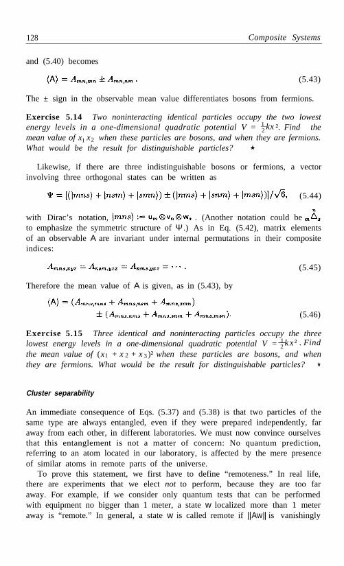
128 Composite Systems
and (5.40) becomes
(5.43)
The ± sign in the observable mean value differentiates bosons from fermions.
Exercise 5.14 Two noninteracting identical particles occupy the two lowestenergy levels in a one-dimensional quadratic potential V = 1
2 kx ². Find themean value of x1 x2 when these particles are bosons, and when they are fermions.What would be the result for distinguishable particles?
Likewise, if there are three indistinguishable bosons or fermions, a vectorinvolving three orthogonal states can be written as
(5.44)
with Dirac’s notation, . (Another notation could beto emphasize the symmetric structure of Ψ .) As in Eq. (5.42), matrix elementsof an observable A are invariant under internal permutations in their compositeindices:
(5.45)
Therefore the mean value of A is given, as in (5.43), by
(5.46)
Exercise 5.15 Three identical and noninteracting particles occupy the threelowest energy levels in a one-dimensional quadratic potential V = 1
2 k x² . Findthe mean value of (x1 + x 2 + x 3)² when these particles are bosons, and whenthey are fermions. What would be the result for distinguishable particles?
Cluster separability
An immediate consequence of Eqs. (5.37) and (5.38) is that two particles of thesame type are always entangled, even if they were prepared independently, faraway from each other, in different laboratories. We must now convince ourselvesthat this entanglement is not a matter of concern: No quantum prediction,referring to an atom located in our laboratory, is affected by the mere presenceof similar atoms in remote parts of the universe.
To prove this statement, we first have to define “remoteness.” In real life,there are experiments that we elect not to perform, because they are too faraway. For example, if we consider only quantum tests that can be performedwith equipment no bigger than 1 meter, a state w localized more than 1 meteraway is “remote.” In general, a state w is called remote if ||Aw|| is vanishingly

Indistinguishable particles 129
small, for any operator A which corresponds to a quantum test in a nearbylocation. It then follows from Schwarz’s inequality (3.18) that any matrix ele-ment involving w, such as ⟨ u, Aw⟩ = ⟨ Au, w⟩ , is vanishingly small. (There is nocontradiction with ⟨ w, w⟩ ≡ 1, because the unit operator is not restrictedto nearby locations.)
We can now show that the entanglement of a local quantum system withanother system in a remote state (as defined above) has no observable effect.Recall that if a quantum system is prepared in a state u, and if we measure anobservable A of that system, the mean value of the result predicted by quantumtheory is ⟨ A ⟩ = ⟨ u, Au⟩ . Suppose now that there is another identical quantumsystem, in a remote state w. The state of the pair is entangled:
(5.47)
where the ± sign is for bosons and fermions, respectively. The operator A,which was used to refer to the “first” system, must now be replaced by a newoperator, namely , which does not discriminate between the twosystems (since the latter are indistinguishable). Yet, we still have
(5.48)
as before, because any matrix element involving A and the remote state w mustvanish. It follows that all predictions on nearby quantum tests are insensitiveto the possible existence of the second particle, far away.
These considerations can be extended to additional particles. Suppose thattwo particles are nearby, and a third one is far away. This will cause no difficultyfor bosons or fermions, as can be seen in the following exercise:
Exercise 5.16 Show that if the state |s⟩ in Eq. (5.46) is localized far awayfrom the states |m ⟩ and |n⟩ , the resulting value of ⟨ A⟩ coincides with that givenby Eq. (5.43).
However, when there are more than two identical particles, new possibilitiesopen up, and symmetries more complicated than those of bosons or fermionsbecome compatible with the indistinguishability principle. These symmetrieswill be discussed in Section 5-5, where it will be shown that they are not com-patible with cluster separability. This will leave us with the Bose-Einstein andFermi-Dirac statistics as the only reasonable alternatives.
Composite bosons and fermions
The remarkable properties of liquid helium are due to the fact that He4 atomscontain an even number of fermions (two electrons, two protons, and two neu-trons) and therefore they behave like elementary bosons, as long as their internalstructure is not probed. Likewise, superconductivity is caused by the formation

130 Composite Systems
of Cooper pairs, whereby two loosely bound electrons behave, in some respects,as a boson. At a deeper level, a proton made of three quarks behaves as anelementary fermion, provided that its internal structure is not probed. Othersimilar examples readily come to the mind.
Let us see why these composite particles act, approximately, as if they werestructureless bosons or fermions. As a simple example, consider a crude modelof the hydrogen atom, consisting of a pointlike proton (mass M, position R )and a pointlike electron (mass m, position r ). Assume that the wave functioncan be factored as
(5.49)
where u involves only the center of mass of the atom, and v describes its internalstructure. Not every wave function has this form, but this is what we wouldobtain by a suitable preparation which selects atoms in their ground state, orin a well defined excited state.
If we now have two such atoms, arbitrarily labelled 1 and 2, their combinedwave function changes sign whenever one swaps the labels of the electrons orthose of the protons. It therefore remains invariant if we swap complete atoms.This leads to the following puzzle: If the atoms were structureless bosons, bothcould be in the same state. What happens when these bosons are made offermions, which cannot be in the same state? To clarify this point, let us writethe combined wave function (apart from a normalization factor) as
(5.50)
where
(5.51)
The wave function (5.50) has all the symmetry properties required by thefermionic nature of the protons and electrons. In particular, Ψ = 0 whenr1 = r2, or when R 1 = R 2. Yet, Ψ clearly does not vanish in general!
Further consideration of this wave function shows that, if the internal statev (R – r ) is highly localized, the first term on the right hand side of (5.50)dominates when R 1 r1 and R 2 r2 , while the second term dominates whenR1 r2 and R 2 r1. These two terms will therefore not interfere, unless thetwo atoms overlap, i.e., R 1 R 2 r1 r2 . Such an overlap of the two atomsoccurs in a region of their configuration space which is exceedingly small, if v islocalized and u is an extended wave function (only if v and u indeed have theseproperties can our four particles be called “two atoms”).
From (5.50), an observable mean value is
(5.52)

Parastatistics 131
The first term in the integrand is just what we would expect for a pair ofelementary bosons, both in the same state ψ. The second term is vanishinglysmall if the extent of u (the “uncertainty” in the position of the center of mass)is much larger than the extent of v (the "size" of each particle). This meansthat the two hydrogen atoms approximately behave as elementary bosons, aslong as they do not appreciably overlap.
Exercise 5.17 Two identical and noninteracting particles are confined to thesegment 0 ≤ x ≤ 1. Both have the same state ψ = e ikx . What is the meanvalue of ( x1 – x 2)2 ? Ans.: 1/6.
We clearly see in this exercise that two particles in the same state may be, onthe average, far away from each other.
Note that swapping the fictitious labels of two identical particles is not thesame as actually swapping their positions and other physical properties. Inthe first case, we have a passive transformation—a mere change of language,like the use of a different coordinate system for describing the same physicalsituation. In the second case, the transformation is active: objects are actuallymoved around. Even if the final conditions appear to be the same as the initialones, the swapping process may cause a phase shift (called the Berry phase5) ,which is experimentally observable. Pairs of particles whose wave function ismultiplied by a nontrivial phase when their positions are swapped have beencalled anyons. 6
5-5. Parastatistics
The symmetrized expressions on the right hand side of Eq. (5.44) representtwo possible configurations of three indistinguishable particles occupying threeorthogonal one-particle states, m ⟩ , n ⟩ , and s ⟩ . However, these two configura-tions do not exhaust all the possible ways of using this set of states. Since thereare six orthogonal three-particle states to start with, there must be four otherorthogonal combinations. The latter too can be chosen so that they have simpleproperties under permutations of the fictitious labels that we arbitrarily attachto the particles in order to perform our calculations. It will now be shown thatthese other possibilities, while mathematically well defined, are unlikely to berealized in nature. Bosons and fermions are the only acceptable types of par-ticles. The reader who is not interested in speculations about the properties ofother types of particles may skip the rest of this section.
A complete classification of all possible symmetrized states is the task ofgroup theory, which is the natural mathematical tool for investigating permu-tations of indistinguishable objects. The group of permutations of n objects is
5M. V. Berry, Proc. Roy. Soc. A 392 (1984) 45.6F. Wilczek, Phys. Rev. Lett. 49 (1982) 957.

132 Composite Systems
called the symmetric group and is denoted by Sn . In the following pages, I shallnot assume that the reader is conversant with the theory of group representa-tions, and all the necessary concepts and techniques will be explained, as theyare needed. Some textbooks on group theory are listed in the bibliography.
Hidden quantum numbers
First, let us put aside a trivial way in which the boson and fermion symmetryrules can be violated. If some physical properties are ignored because they arenot discerned by our quantum tests, the states resulting from these incompletetests are not pure. These states are represented by density matrices of ranklarger than 1, and the elementary symmetrization method used in Eq. (5.44) isnot applicable. In this case, however, it is always possible to restore the usualsymmetry rules by introducing new quantum numbers, even if the latter are(perhaps temporarily) not experimentally accessible.
For example, when the quark model was first introduced in particle physics,it had the unpleasant feature that three identical u-quarks, each one with spin
–
,were used to make one ∆+ + particle, which had spin3 . This implied that the2three u -quarks had the same spin state, in contradiction to the spin-statisticstheorem, which wants spin particles to be fermions. Likewise, three d-quarksmade one ∆ – , and three s-quarks made one Ω– , both having spin . The puzzlewas solved by attributing to quarks a new property, called “color,” with threepossible values, and assuming that the three quarks making a baryon alwayswere in an antisymmetric color state—and therefore their spin state had tobe symmetric. However, before the concept of colored quarks gained generalacceptance, serious consideration was given to the possibility that quarks mightsatisfy parastatistics, that is, permutation rules different from those of bosonsand fermions. The simplest example of such rules is discussed below, for thecase of three indistinguishable particles.
Three indistinguishable particles
The bosonic state in Eq. (5.44)is invariant under any exchange of the particlelabels. The fermionic state is invariant under cyclic permutations of the labels,and it changes sign if any two labels are swapped. These various permutationscan be visualized by attaching the fictitious labels to the vertices of an equilat-eral triangle. Cyclic permutations become rotations of the triangle around itscenter, by angles of ±2π⁄3, and label swappings are reflections of the trianglethrough one of its three medians. Our next task is to find other quantum states,besides those of Eq. (5.44), having simple transformation properties under theserotations and reflections. Let us introduce the following notations:
(5.53)
–32
–32–32
–12
–12

Parastatistics 133
Note thatA convenient pair of states, with simple transformation properties, is
Exercise 5.18 Show that Ψ+ and Ψ– are normalized, orthogonal to eachother, and orthogonal to the boson and fermion states of Eq. (5.44).
Under a cyclic permutation, , we have and. These transformations can be written as
where Ψ is a column vector with components Ψ+ and Ψ – . On the other hand,an exchange of the first two labels, , gives , or
Any other permutation of the particle labels can be obtained by combining thesetwo operations, and is therefore represented by products of these two matrices.
The set of matrices that correspond to all these permutations (includingthe unit matrix for the identity transformation) is called a representation o fthe symmetric group. Note that these matrices are unitary, and that the onlymatrix which commutes with all of them is the unit matrix (or a scalar mul-tiple thereof). The last property characterizes an irreducible representation ofa group. (Contrariwise, a reducible representation consists of block diagonalmatrices, all identically structured in submatrices of the same size, so that eachset of submatrices is by itself a representation of the group.)
Bosons correspond to a trivial unitary representation of the symmetric group:the transformation matrices are one-dimensional, and all of them are equalto 1. This representation is called D(0) . (The notations used here are those ofWigner’s book, listed in the bibliography.) Fermions also correspond to a one-
dimensional representation, which is called : the matrices corresponding toeven permutations are equal to 1, and those corresponding to odd permutationsare -1. The symmetric group has no other one-dimensional representation. Itcan be shown that all its other representations are multidimensional. Moreover,it can be shown that, for any finite group, the sum of the squares of the dimen-sions of all the inequivalent irreducible representations is equal to the numberof group elements (which is n! for the symmetric group Sn ).
In the particular case of S3 that we are investigating now, we have just found atwo-dimensional representation which consists of the matrices in Eqs. (5.55) and(5.56), and all the products of these matrices. This irreducible representationis called D(1) . There can be no further (inequivalent) representation, because
(5.54)
(5.55)
(5.56)

134 Composite Systems
1 + 1 + 2 = 3!, which is the number of group elements. On the other hand, we2
have so far used only four orthonormal states: the bosons and fermions givenby Eq. (5.44),and the Ψ + and Ψ – states in Eq. (5.54), which form a closed setunder all permutations. Therefore there must be another orthonormal pair ofstates, which also transforms under permutations with the aid of the matricesof the D (1) representation (but which does not mix with Ψ ± ).
It is not difficult to find the two missing states. They can be taken as
(5.57)
Exercise 5.19 Verify that Φ + and Φ – are orthogonal to the boson, fermion,and Ψ± states, and that they behave exactly as Ψ+ and Ψ– under permutationsof the particle labels.
Exercise 5.20 Show that, for any real a and β, the four states
and
(5.58)
(5.59)
are mutually orthogonal, and that each pair, Ξ ± and ± , has the same trans-formation properties as Ψ ± and Φ ± under permutations of the particle labels.
Exercise 5.21 Show that the pair of orthonormal states
and (5.60)
transforms according to
and
if (5.61)
if (5.62)
The last exercise shows that all six matrices of the D (1) representation can bemade real by a unitary transformation of the basis. (Different representationsof the same group, related by a unitary transformation of the basis, are said tobe equivalent. ) Since the new D (1) matrices no longer involve i, the coefficientsof i and of –i in the vectors Λ ± are not mixed by these matrices, and thereforethey transform independently. You may verify that the two pairs of vectors
(5.63)

Parastatistics 135
and
(5.64)
are mutually orthogonal, and that each pair transforms, without mixing withthe other, as in Eqs. (5.61) and (5.62).
Inequivalent bases can be experimentally distinguished
This wealth of equivalent D (1) representations raises a fundamental question:Given that the particles cannot be individually identified, are there quantumtests able to distinguish from each other the various states, , etc.?It is obvious that states which can be transformed into each other by relabellingthe particles, such as Ψ+ and Ψ – , or any linear combination thereof (for exam-ple, Λ ± ) cannot be distinguished by any test. Indeed, the mean value of anyobservable A is the same,
(5.65)
because a relabelling of the particles is represented by a unitary transformation,, under which A is invariant: A = UAU† .
On the other hand, bases that cannot be converted into each other by merelyrelabelling the particles, such as Ψ± and Φ ± , are experimentally distinguishable.For instance, the operator
(5.66)
is invariant under a relabelling of the particles; all linear combinations of theΨ± states are eigenvectors of that operator (with eigenvalue +1); those of Φ±
states also are eigenvectors (eigenvalue –1);and the boson and fermion statesin Eq. (5.44)are eigenvectors too (eigenvalue 0). A physical realization of theoperator in (5.66)would therefore allow us to verify whether triads of identicalparticles are of type Ψ , or Φ , or none of these.
As a concrete example, consider the symmetric expression
(5.67)
where x, y and z are the coordinates of three identical particles, and px , p y andpz are the conjugate momenta. Let the three states,|m ⟩ , | n ⟩ , and | s⟩ , be thoseof a harmonic oscillator, with the ground state labelled 0 (not 1). We then have(in natural units, including = 1),
(5.68)

136 Composite Systems
It follows that (xp – p x )m n = i δmn , as is well known, and
(5.69)
Therefore the operator A, given by Eq. (5.67), has a nonvanishing mean value ifthe states m ⟩, n and s ⟩ correspond to three consecutive levels—in any order.For example, let us take them as 0⟩, 1⟩ a n d 2⟩ . We have
(5.70)
(5.71)
and you are invited to verify that
and
while ⟨ A⟩ = 0 for bosonic and fermionic states.
Exercise 5.22 Find the mean value of the operator A in Eq. (5.67) for thestates Ξ ± , ± , and Λ ± , which were defined in the preceding exercises. *
These results show beyond doubt that, if there were particles which obeyedparastatistics rules, that property would have observable consequences.
Suppose now that we have three particles of the Ψ ± type. That is, we havedetermined experimentally that they are neither Φ , nor± ± , etc. On theother hand, we have no experimental way of differentiating Ψ+ from Ψ– (orfrom linear combinations thereof, such as Λ± ) because the particles are indis-tinguishable. These states can be transformed into each other by relabellingthe particles, and all mean values, such as ⟨ A ⟩ , are the same for all of them. Itfollows that the physical state of our three-particle system is an equal weightmixture of and This mixture is represented by a density matrixwhich is proportional to the unit matrix (in the subspace spanned byΨ + andΨ–), and is therefore invariant under the unitary transformations correspond-ing to permutations of the particles. We have a mixture, rather than a purestate, because of the inaccessibility of some data—namely, the conceptual labelsattached to the indistinguishable particles.
Cluster inseparability
The above considerations can be generalized to multidimensional irreduciblerepresentations of S n , for n > 3. The latter have the property that, when wedescend7 from S n to its subgroup S n –1 (for instance if one of the particles is sodistant that we ignore it and permute only the labels of the n –1 other particles),all the irreducible representations of Sn become reducible representations ofSn –1. This too has observable consequences, that will now be discussed.
7 H. Weyl, Theory of Groups and Quantum Mechanics, Methuen, London (1931) [reprintedby Dover] p. 390.

Fock space 137
Returning to the case of three particles, assume that the m ⟩ and n⟩ statesare localized in our laboratory, while the s ⟩ state is remote, localized on theMoon, say. The question may now be raised: if three particles obey the D (1)
symmetry, what happens when we swap the labels of only two particles ofthe same species (More generally, if n particles belong to a given irreducible?representation of S n , what is the representation for a subset of n – 1 particles?)We have already investigated a similar question in the case of three bosons orfermions (see Exercise 5.16) and we then found the intuitively obvious resultthat if one of the three particles is remote, the two others still behave as bosonsor fermions, respectively.
However, for three particles obeying the D (1) symmetry, the situation is morecomplicated. For example, if they are of type Ψ± , we have, instead of Eq. (5.46),
(5.72)
Exercise 5.23 Show from Eq. (5.54) that the matrix elements Amns,snm andA mns,smn are complex conjugate, and verify Eq. (5.72).
On the other hand, for three particles of type Φ ± , we have a different result,which looks like (5.72), but with Other bases, which also lead to thesame D (1) representation, or to unitarily equivalent ones, give for the observablemean value ⟨ A⟩ still other results. None of these results has the desired propertyof reducing to the boson or fermion symmetry rules, if one of the three occupiedstates is remote, and only the two others are accessible.
This leads to a paradoxical situation. We know that two indistinguishableparticles behave either as bosons, or as fermions. On the other hand, if we havesuch a pair of particles here, we can never be sure that there is no third particleof the same kind elsewhere (e.g., on the Moon). The mere existence of thatthird particle would make the trio obey D (1) statistics—which implies, for thetwo particles in our laboratory, an improperly symmetrized ⟨A⟩ , unlike that inEq. (5.43) which was valid for bosons or fermions. Since it is hardly conceivablethat observable properties of the particles in our laboratory are affected by thepossible existence on the Moon of another particle of the same species, we areforced to the conclusion that only Bose-Einstein or Fermi-Dirac statistics areadmissible for indistinguishable systems.
5-6. Fock space
An efficient way of writing completely symmetric or antisymmetric state vectorsis the use of a Fock space. This is a new notation, which also allows theintroduction of states where the number of particles is not definite. Such statesnaturally occur whenever particles can be produced or absorbed. For example,if an atom is prepared in an excited energy state from which it can decay byemission of a photon, the quantum state after a finite time will be a linear

138 Composite Systems
superposition of two components, representing an excited atom, and an atom inits ground state accompanied by a free photon; the number of photons presentin that quantum system is indefinite. We thus need a mathematical formalismwhich is able to represent situations of that kind, and is more powerful thanordinary quantum mechanics, which describes only permanent particles.
Raising and lowering operators
We now define a raising operator by the property that the vectoris normalized and represents a single particle in state eµ . (The term creationoperator and the notation are also commonly used.) The operator which isadjoint to is written and is a lowering operator, because
Assume for simplicity that there is only one kind of particle, and that thephysical system has a nondegenerate vacuum state, in which no particles arepresent.8 That state is denoted byΨ0 (or 0⟩ , in the Dirac notation). It is thenormalized ground state of the system, and it should not be confused with thenull vector 0, which does not represent a physical state.
(5.73)
and therefore
(5.74)
so that maps the one particle state eµ into the vacuum state. (The termsdestruction, or annihilation operator, and the notation a µ, without a super-script, are also commonly used for )
We shall henceforth assume that (except for normalization) the operatoradds a particle in state eµ to any state (not only to the vacuum state) andtherefore its adjoint removes such a particle. In particular,
(5.75)
is the null vector, because removing a particle from the vacuum produces anunphysical state.
Fermions
Two fermions cannot occupy the same state. We therefore writesince this expression is unphysical. More generally,
(5.76)
even when this operator acts on a non-vacuum state.8 This assumption is not as obvious as it may seem. Quantum field theory involves an infinite
number of degrees of freedom and allows, in some cases, the existence of degenerate vacua. TheFock space formalism, discussed here, is not applicable to these situations.

Fock space 139
We likewise have for any e v orthogonal to eµ , and moreover, forthe state represented by the unit vector we haveCombining all these equations, we obtain
(5.77)
which generalizes Eq. (5.76). The raising operators and are said to anti-commute. The lowering operators, which are their adjoints, also anticommute:
(5.78)
The state vector
(5.79)
represents two fermions occupying the orthogonal states eµ and e v . With thisnew notation, no fictitious labels need to be attached to the two particles.However, we can still swap the labels µ and v of the occupied states, and thenthe entire vector changes its sign, as seen in (5.79). This property is readilygeneralized to three or more fermions: the complete antisymmetrization of thestate vector is automatically included in the Fock formalism.
It is convenient to define a number operator,
(5.80)
It follows from Eqs. (5.75) and (5.74), respectively, that the eigenvalues of Nµare 0 and 1, since
and (5.81)
Exercise 5.24 Show that the operator has the same eigenvectors asNµ , but with eigenvalues 1 and 0, respectively, and therefore
(5.82)
Show, more generally, that
(5.83)
Hint: Consider the raising and lowering operators,for the normalized state eθ , with an arbitrary value of the mixing angle θ.
From (5.83), it follows that
(5.84)

140 Composite Systems
because the exchange of two anticommuting operators involves two changes ofsign, and therefore pairs of anticommuting operators commute.
Bosons
The treatment of bosons is simpler in some respects, and more complicatedin others, than that of fermions. It is simpler because the sign of the statevector does not change when occupied states are swapped. On the other hand,each state can be occupied by an arbitrary number of particles. A completeorthonormal basis can be written as where n µ is the numberof particles in state eµ . We may define a number operator N µ , for that state,b y
nα nβ ... n µ ... ⟩ ,
(5.85)
It then follows from the definition of the raising and lowering operators that
(5.86)
or, more generally,
(5.87)
The raising and lowering operators for bosons commute,
(5.88)
instead of anticommuting like those of fermions, because bosonic state vectorsdo not change sign if state labels are swapped.
Equation (5.87) can also be written as
(5.89)
Since the basis is complete, this gives the operator equation
(5.90)
from which it is easily shown thatWe have not yet normalized the raising and lowering operators The
preceding relations only say that, in the basis where Nµ is diagonal, the matriceshave their nonvanishing elements in the adjacent diagonals:
and (5.91)
Therefore, It is convenient to choose so that
(5.92)

Fock space 141
has the same form as the number operator for fermions. It also follows fromthe preceding equations that and therefore, for any pair oforthogonal states,
(5.93)
This is a commutation relation, instead of the anticommutation relation (5.83)that was valid for the fermionic raising and lowering operators.
It follows from (5.90) and (5.91), with that
Therefore, the normalized basis states in Fock space are
Exercise 5.25 Show that
(5.94)
(5.95)
(5.96)
Exercise 5.26 Show that
and (5.97)
satisfy the canonical commutation relation
Exercise 5.27 Try again to solve Exercise 2.20 (page 47) by using Fock spacemethods. Hint: Let a + and b+ be the creation operators for photons polarizedalong the x- and y-axes, respectively. The operators corresponding to axesrotated by an angle θ are and Thereforethe state with N photons polarized along θ, and N photons along θ + π / 2, i s
(5.98)
Show that, if is small and N is large, we haveso that the angular resolution attainable by an ideal measurement is about
*
Parafermions
The Fock space formalism can be adapted to represent hypothetical particleshaving a number operator with eigenvalues 0, . . . , M (ordinary fermions cor-respond to M = 1.) Indeed, any matrix of order M + 1, with nonvanishingelements given by (5.91), is a raising operator which satisfies

142 Composite Systems
(5.99)
For example, a smooth interpolation between fermions (M = 1) and quasi-bosons (M → ∞ ) is obtained from
Exercise 5.28 Show that Eq. (5.99) is satisfied by (5.100), and moreover that
and therefore
(5.100)
(5.101)
The expression on the left hand side of this equation is the number operatorNµ , with eigenvalues 0, . . . , M.
The generalization of Eq. (5.99) to products of raising operators belonging todifferent states can be obtained by considering transformations to other ortho-normal bases. The transformation law (3.2) gives
(5.102)
where C µm is an arbitrary unitary matrix. Because of this arbitrariness, wehave, in general,
(5.103)
where each term is a product of M + 1 raising operators, and the sum includesall the permutations of the indices mn . . . s. This relationship—which dependssolely on the property of postulated in Eq. (5.99), not on its particularimplementation in Eq. (5.100)—imposes an antisymmetry property on statevectors, when there are more than M particles. However, this antisymmetry isnot restrictive enough for a smaller number of particles.
This alternative approach to parastatistics is just another way of showingthe difficulties that were already mentioned in the preceding section.
5-7 . Second quantization
Some composite quantum systems contain a large number of indistinguishableparticles: heavy nuclei, solids, neutron stars, are typical examples. A methodcalled second quantization, originally devised for use in quantum field theory,allows us to treat these large assemblies of particles without having to specifyhow many particles are actually involved. This is made possible by using theFock basis given by (5.95). We shall now learn to write ordinary operators, likethose for kinetic energy, or potential energy, in that new basis.

Second quantization 143
One-particle operators
Consider an additive dynamical variable, such as kinetic energy, or angularmomentum, which is represented in quantum mechanics by an operator A(q, p)when there is a single particle. If there are N indistinguishable particles, thetotal value of that variable is
(5.104)
We are interested in the matrix elements of A between Fock states, which area complete orthonormal set labelled by occupation numbers nµ .
In ordinary quantum mechanics, where particles are not allowed to appear ordisappear (as they can do in quantum field theory) an operator acting on a statevector may change the occupation numbers n µ of individual basis states, butit cannot change In particular, A does not change the total number ofparticles. Therefore, the observable A has nonvanishing matrix elements onlybetween Fock states with the same total number of particles, because stateswith different numbers of particles are orthogonal.
Let us now choose a one-particle basis in which A (q, p) is diagonal. Withthat basis, even the individual occupation numbers nµ do not change when thediagonalized operator A acts on a Fock state, and we have
(5.105)
This can be written as an operator equationRecall that this equation holds only in the basis where A is diagonal. Its formin any other basis (denoted as usual by Latin indices) can be obtained from thetransformation law (5.102), and its Hermitian conjugate which is
(5.106)
We have
(5.107)
Since A is diagonal in the Greek basis, the parenthesis on the right hand sideof (5.107) can also be written as
(5.108)
where use was made of the transformation law for matrices (3.46). Thus, finally,
(5.109)

144 Composite Systems
The remarkable property of this expression for A is that it makes no explicitreference to the total number of particles, while that information was needed forwriting Eq. (5.104). This is the advantage of the “second quantized” notation,with respect to the ordinary, “first quantized” one.
Exercise 5.29 Show that the generalization of Eq. (5.105) to a general basiswhere Aµv is not diagonal is
(5.110)
It is instructive to verify the agreement of Eq. (5.110) with the resultthat can be obtained, laboriously, by means of the first quantized formalism.Assume for simplicity that only the two states eµ and e v are occupied. LetN = nµ + n v . The state vector Ψ is a symmetrized sum of differentterms that correspond to inequivalent ways of attributing states eµ and ev tothe particles. Since all these terms are orthogonal, the normalization factor is
From the definition of matrix elements,+ irrelevant terms), we see that the vector A Ψ contains:
1) the same terms as in Ψ, with unaltered occupation numbers, but multipliedby a coefficient
2) terms with a coefficient Aµv , in which one particle switched from ev to e µ .The number of these terms is
(5.111)
together with the coefficient (nµ + 1) on the right hand side of (5.111),exactly gives the square root in Eq. (5.110).
so that each symmetrized set of these new terms occurs (n µ + 1) times. Thenew normalization factor is Comparing the old
and new normalizations, we get an extra coefficient which,
3) and likewise for µ ↔ v .
Two-particle operators
A similar treatment applies to additive two-particle operators, such as two-bodyCoulomb interactions. In the ordinary (first quantized) notation, we have
When this operator acts on a Fock state, it may change the occupation numbersof at most two one-particle states, and it can therefore be written as
(5.112)

Second quantization 145
(5.113)
Note that the raising operators stand on the left of the lowering operators. Thisis called a normal ordering. Any other ordering can be obtained by using the(anti)commutation relations (5.83) and (5.93); the result differs from (5.113)by terms having only one raising and one lowering operator (or none at all),that is, by a one-particle operator (or a scalar). This ordering arbitrariness isrelated to a trivial ambiguity in the definition of a two-particle operator: anexpression such as B (q i p i q j p j) remains a two-particle operator if one adds, , ,to it a sum of two one-particle operators.
It will now be shown that the coefficient in (5.113) is the ordinarytwo-particle matrix element,
(5.114)
where the minus sign is for fermions, and where
(5.115)
and
(5.116)
are the symmetrized state vectors given by Eqs. (5.37) and (5.38). Consider forexample the effect of B on a two-particle state eρσ (with ρ ≠ σ ). We have
(5.117)
Repeated use of the (anti)commutation relations (5.83) and (5.93), togetherwith gives
(5.118)
whence
(5.119)
which is just another way of writing Eq. (5.114).
Exercise 5.30 Compute explicitly Hint: Use thecommutation relation (5.96).
Exercise 5.31 Compute explicitly *

146 Composite Systems
Quantum fields
Let the abstract Hilbert space vectors eµ be represented by functions uµ (r, t),which satisfy the orthonormality and completeness relations
(5.120)
and
(5.121)
Note that the same parameter t accompanies both r' and r " .Under a unitary transformation of the basis e µ , given by Eq. (3.2), we have
(5.122)
It then follows from the transformation law (5.106) that the operators
and (5.123)
are invariant under a unitary transformation of the basis, produced by thematrix C µm . They are not invariant, of course, if we choose a different set oforthonormal functions uµ (r,t) for representing the same physical state eµ .
If all the functions u µ (r, t ) happen to satisfy a partial differential equation(the same equation for all µ ), the operator ψ (r, t) also satisfies that partialdifferential equation. In that respect, it behaves like a field in classical physics,and for that reason it is called a “quantum field.” In particular, if the functionsuµ (r, t ) obey a Schrödinger equation, the field ψ (r, t ) also obeys that equation.This is the origin of the term “second quantization”: The old quantum wavefunction (for a single particle) becomes an operator, and the new state vector(for an indefinite number of particles) is given by a combination of Fock states.
The quantum fields ψ and ψ * have (anti)commutation relations9
(5.124)
and
(5.125)
by virtue of Eqs. (5.83), (5.93), and (5.121). The singular nature of this(anti)commutator is related to that of the fields themselves: The sums in (5.123)do not converge, and the quantum fields ψ and ψ* actually are operator valueddistributions, as explained at the end of Chapter 4.
Operators that were defined in Fock space, such as A and B, can now bewritten in terms of fields. We have
9 The symbol [A, B]± means AB ± BA.

Bibliography 147
(5.126)
Likewise,
(5.127)
Exercise 5.32 Take A = 1 and show that the operator for the total numberof particles is
Exercise 5.33 Check that the factor ordering in Eq. (5.127) is the correctone for fermions (it is of course irrelevant for bosons).
5-8 . Bibliography
Group theory
The theory of group representations is an essential mathematical tool in many ap-plications of quantum mechanics. The reader who is not already familiar with thissubject is urged to get acquainted with this powerful technique. The classic treatise is
E. P. Wigner, Group Theory and Its Application to the Quantum Mechanicsof Atomic Spectra, Academic Press, New York (1959).
This book is an expanded translation of Gruppentheorie und ihre Anwendung aufQuantenmechanik der Atomspektren, Vieweg, Braunschweig (1931). A more recentintroductory text, with applications to molecular and solid state physics, is
M. Tinkham, Group Theory and Quantum Mechanics, McGraw-Hill, NewYork (1964).
Schmidt’s theorem
E. Schmidt, “Zur Theorie der linearen und nichtlinearen Integralgleichun-gen,” Math. Ann. 63 (1907) 433.
A. Peres, “Higher order Schmidt decompositions,” Phys. Letters A 202 (1995)16.
Necessary and sufficient conditions are given for the existence of a Schmidt decom-position involving more than two subspaces.
Many-Body Theory
A. A. Abrikosov, L. P. Gor’kov, and I. Ye. Dzyaloshinskii, Quantum FieldTheoretical Methods in Statistical Physics, Pergamon, Oxford (1965) [transl.from the Russian].
A. L. Fetter and J. D. Walecka, Quantum Theory of Many-Particle Systems,McGraw-Hill, New York (1971).

Chapter 6
Bell’s Theorem
6 - l . The dilemma of Einstein, Podolsky, and Rosen
The entangled states introduced in Chapter 5 raise fundamental issues, whichwere exposed by Einstein, Podolsky, and Rosen (hereafter EPR) in a classicarticle1 entitled “Can Quantum Mechanical Description of Physical Reality BeConsidered Complete?”. In that article, the authors define “elements of physicalreality” by the following criterion: If, without in any way disturbing a system,we can predict with certainty . . . the value of a physical quantity, then thereexists an element of physical reality corresponding to this physical quantity. Thiscriterion is then applied by EPR to a composite quantum system consisting oftwo distant particles, with an entangled wave function
(6.1)
Here, the symbol δ does not represent a true delta function, of course, but anormalizable function with an arbitrarily high and narrow peak; and L is alarge distance—much larger that the range of mutual interaction of particles 1and 2. The physical meaning of this wave function is that the particles havebeen prepared in such a way that their relative distance is arbitrarily close to L,and their total momentum is arbitrarily close to zero. Note that the operatorsx1 – x 2 and p 1 + p2 commute.
In the state ψ, we know nothing of the positions of the individual particles(we only know their distance from each other); and we know nothing of theirindividual momenta (we only know the total momentum). However, if wemeasure x1, we shall be able to predict with certainty the value of x 2 , withouthaving in any way disturbed particle 2. At this point, EPR argue that “since atthe time of measurement the two systems no longer interact, no real change cantake place in the second system in consequence of anything that may be done tothe first system. ” Therefore, x 2 corresponds to an “element of physical reality,”as defined above.
1 A. Einstein, B. Podolsky, and N. Rosen, Phys. Rev. 47 (1935) 777.
148

The dilemma of Einstein, Podolsky, and Rosen 149
Nathan Rosen, working inhis office at Technion, 55years after he co-authoredthe famous EPR article.
On the other hand, if we prefer to perform a measurement of p1 rather than ofx 1, We shall then be able to predict with certainty the value of p2, again withouthaving in any way disturbed particle 2. Therefore, by the same argumentas above, p2 also corresponds to an “element of physical reality.” However,quantum mechanics precludes the simultaneous assignment of precise values toboth x 2 and p 2 , since these operators do not commute, and thus EPR “areforced to conclude that the quantum mechanical description of physical realitygiven by wave functions is not complete.” However, they prudently leave openthe question of whether or not a complete description exists.
Bohr’s reply
Soon after its publication, EPR’s article was criticized by Bohr.2 Let us exam-ine the points of agreement and disagreement. Bohr did not contest the validityof counterfactual reasoning. He wrote: "our freedom of handling the measur-ing instruments is characteristic of the very idea of experiment . . . we have acompletely free choice whether we want to determine the one or the other ofthese quantities . . . ” Thus, Bohr too found it perfectly legitimate to considercounterfactual alternatives. He had no doubt that the observer had free willand could arbitrarily choose his experiments.
On the other hand, Bohr disagreed with EPR’s interpretation of the notionof locality. He readily conceded that “there is no question of a mechanicaldisturbance of the system under investigation” [due to the measurement of theother, distant system], but he added: “there is essentially the question of aninfluence on the very conditions which define the possible types of predictionsregarding the future behavior of the system.”
Bohr gave to his point of view the name “principle of complementarity.”Its meaning is that some types of predictions are possible while others arenot, because they are related to mutually incompatible tests. For example, in
2N. Bohr, Phys. Rev. 48 (1935) 696.

150 Bell’s Theorem
the situation described by EPR, the choice of the experiment performed onthe first system determines the type of prediction that can be made for theresults of experiments performed on the second system. On the other hand,no experiment, performed on the second system by an observer ignorant of theabove choice, would reveal the occurrence of a “disturbance” to that system,thereby disclosing what the choice of the first experiment had been.
According to Bohr, each experimental setup must be considered separately.In particular, no conclusions can be drawn from the comparison of possibleresults of mutually incompatible experiments (i.e., those having the propertythat the execution of any one of these experiments precludes the execution ofthe others). Bohr’s argument did not convince Einstein who later wrote, in hisautobiography:3
. . . it becomes evident that the paradox forces us to relinquish one of thefollowing two assertions:
(1) the description by means of the ψ-function is complete,(2) the real states of spatially separated objects are independent of eachother.
In Einstein’s mind, the second of these assertions was indisputable. Hewrote:4 “On one supposition we should, in my opinion, absolutely hold fast:the real factual situation of the system S2 is independent of what is done withthe system S1, which is spatially separated from the former.” This physicalprinciple has received the name Einstein locality.
Spin systems
A simpler example of the same dilemma, involving only discrete variables, wasproposed by Bohm,5 and became since then the basis of most discussions ofthe so-called “EPR paradox.” Consider the decay of a spinless system into apair of spin particles, such as (this decay mode of π0 is rare, butit actually occurs). After the decay products have separated and are very farapart, we measure a component of the spin of one of them. Suppose that Sx ofthe electron is measured and found equal to Then, we can be sure that S x
of the positron will turn out equal to if we measure it; in other words, weknow that the positron is in a state with Moreover, it must havebeen in that state from the very instant the positron was free, since it did notinteract with other particles.
On the other hand, we could have measured Sy of the electron and, by thesame argument, Sy of the positron would have been definite; and likewise for Sz .
3 A. Einstein, in Albert Einstein, Philosopher-Scientist, ed. by P. A. Schilpp, Library ofLiving Philosophers, Evanston (1949) p. 682.
4 A. Einstein, ibid., p. 85.5 D. Bohm, Quantum Theory, Prentice-Hall, New York (1951) p. 614.
–12
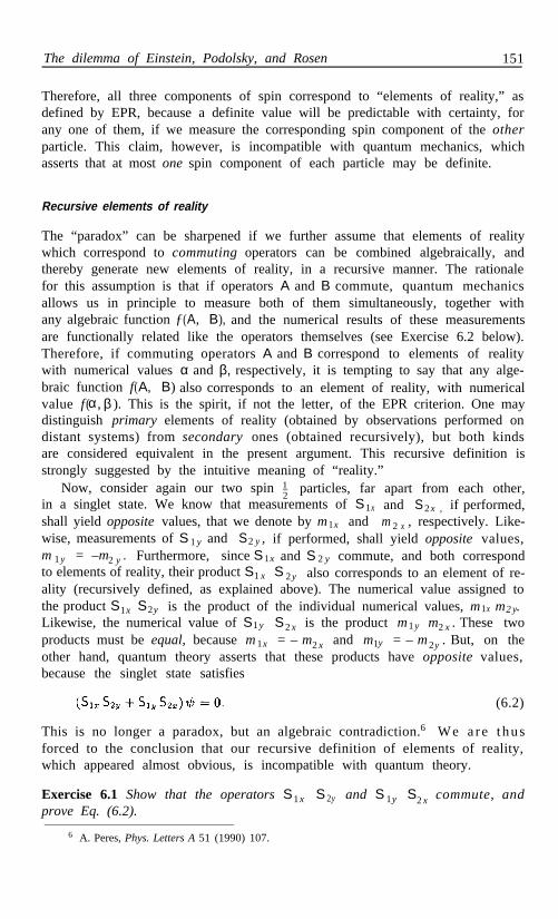
The dilemma of Einstein, Podolsky, and Rosen 151
Therefore, all three components of spin correspond to “elements of reality,” asdefined by EPR, because a definite value will be predictable with certainty, forany one of them, if we measure the corresponding spin component of the otherparticle. This claim, however, is incompatible with quantum mechanics, whichasserts that at most one spin component of each particle may be definite.
Recursive elements of reality
The “paradox” can be sharpened if we further assume that elements of realitywhich correspond to commuting operators can be combined algebraically, andthereby generate new elements of reality, in a recursive manner. The rationalefor this assumption is that if operators A and B commute, quantum mechanicsallows us in principle to measure both of them simultaneously, together withany algebraic function ƒ(A, B), and the numerical results of these measurementsare functionally related like the operators themselves (see Exercise 6.2 below).Therefore, if commuting operators A and B correspond to elements of realitywith numerical values α and β, respectively, it is tempting to say that any alge-braic function f(A, B) la so corresponds to an element of reality, with numericalvalue f (α, β ). This is the spirit, if not the letter, of the EPR criterion. One maydistinguish primary elements of reality (obtained by observations performed ondistant systems) from secondary ones (obtained recursively), but both kindsare considered equivalent in the present argument. This recursive definition isstrongly suggested by the intuitive meaning of “reality.”
Now, consider again our two spin particles, far apart from each other,in a singlet state. We know that measurements of S1x and S2x , if performed,shall yield opposite values, that we denote by m1x and m 2 x , respectively. Like-wise, measurements of S 1y and S2 y , if performed, shall yield opposite values,m 1y = –m2 y . Furthermore, sinceS 1x and S 2 y commute, and both correspondto elements of reality, their product S1 x S 2y also corresponds to an element of re-ality (recursively defined, as explained above). The numerical value assigned tothe product S1x S2y is the product of the individual numerical values, m1x m2 y.Likewise, the numerical value of S1y S2x is the product m1y m2 x . These twoproducts must be equal, because m1x = – m2x and m1y = – m2y . But, on theother hand, quantum theory asserts that these products have opposite values,because the singlet state satisfies
(6.2)
This is no longer a paradox, but an algebraic contradiction.6 We are thusforced to the conclusion that our recursive definition of elements of reality,which appeared almost obvious, is incompatible with quantum theory.
Exercise 6.1 Show that the operators S1x S 2y and S 1y S2x commute, andprove Eq. (6.2).
6 A. Peres, Phys. Letters A 51 (1990) 107.
–12

152 Bell’s Theorem
Exercise 6.2 Show that if a state ψ is prepared in such a way that A ψ = αψand Bψ = βψ, then Note that this result is valid even ifA and B do not commute, but merely happen to have a common eigenvector ψ .
Three particle model
A similar contradiction was derived by Mermin7 for a three particle system,without the use of any debatable extension of the EPR criteria. (Mermin’sargument is a simplified version of another one, with four particles, due toGreenberger, Horne, and Zeilinger.8 )
The three spin particles are prepared in an entangled state
(6.3)
where the coordinate space wave function ƒ (r 1 , r 2 , r3) has a form ensuringthat the particles are widely separated, and where the spin states u and v areeigenstates of σz , satisfying
(6.4)
It is easily seen that ψ is an eigenfunction of several operators:
(6.5)
and
(6.6)
Exercise 6.3 Verify the above equations and show that these four operatorscommute. Moreover show that
(6.7)
either σx or σ y , without disturbing the other particles. The results of these
The minus sign in (6.7)is crucial, as will soon be seen.The EPR argument now runs as follows. We may measure, on each particle,
measurements will be called mx or m y , respectively. From (6.6), we can predictwith certainty that, if the three σ x are measured, the results satisfy
(6.8)
7 N D Mermin, Physics Today 43 (June 1990) 9; Am. J. Phys. 58 (1990) 731.. .8 D. M. Greenberger, M. Horne, and A. Zeilinger, in Bell’s Theorem, Quantum Theory, and
Conceptions of the Universe, ed. by M. Kafatos, Kluwer, Dordrecht (1989) p. 69.
–12

The dilemma of Einstein, Podolsky, and Rosen 153
Therefore each one of the operators σ 1x , σ 2 x , and σ 3 x corresponds to an EPRelement of reality, because its value can be predicted with certainty by perform-ing measurements on the two other, distant particles.
However, it also follows from (6.5) that we can predict with certainty thevalue of σ 1x by measuring σ2y and σ3y rather than σ2 x and σ 3x . We have
(6.9)
and likewise, by cyclic permutation,
(6.10)
and
(6.11)
The product of the last four equations immediately gives a contradiction.There is a tacit assumption in the above argument, that m 1x in Eq. (6.8)
is the same as m 1 x in Eq. (6.9), in spite of the fact that these two ways ofobtaining m1x involve mutually exclusive experiments—measuring σ2 x a n d σ 3x ,or measuring σ 2 y and σ 3y . This tacit assumption is of counterfactual nature,and cannot be experimentally verified. It obviously adheres to the spirit ofthe EPR article—it is almost forced upon us by the intuitive meaning of theword “reality”—but it is open to the same criticism that Bohr expressed in hisresponse to Einstein, Podolsky, and Rosen.
Einstein locality and other relativistic considerations
The paradoxes—or algebraic contradictions—resulting from the apparentlyreasonable criteria proposed by EPR, prompt us to reexamine more carefullytheir argument: If . . . we can predict with certainty . . . Who are “we”?
In Bohm’s singlet model, the observer who measures S1 x and findsknows that if the other observer measures (or has measured, or will measure)S2x , she9 must find the opposite result, However, this knowledge isuseless (it is devoid of operational meaning) because the two observers are farapart. The only thing that the first observer can do is to send a message tothe second one, telling her that she can verify that S 2 x is provided thatshe has not yet disturbed her particle by measuring another component of spin,before she received that message.
Now assume that, unbeknownst to the first observer, she measures S2y andfinds the result say. Can there be any paradox here? Conceptual difficul-ties may indeed arise if you demand that every physical system, such as our pairof particles, has, at every instant, a well defined quantum state (some authors
9 When two observers are involved, I shall call the second one “she” rather than “he” (seefootnote on page 12).

154 Bell’s Theorem
would like the entire Universe to have a quantum state). To illustrate this diffi-culty, let our two observers be attached to different Lorentz frames, as shown inFig. 6.1. They recede from each other, with a constant relative velocity. Thus,in each one of the Lorentz frames, the test performed by the observer who is atrest appears to occur earlier than the test performed by the moving observer.If the first observer got a bad education in quantum theory and believes thatthe pair of particles has, at each instant, a definite wave function, he will saythat the singlet state, which existed for t 1 < 0, collapsed into an eigenstate ofS1x and of S2x , for t1 > 0. In the same vein, the second observer may say thatthe singlet state held for t2 < 0, and thereafter collapsed into an eigenstate ofS1y and of S2y , as a result of her test.
Fig. 6.1. In this spacetime diagram, the origins of the coordinate systemsare the locations of the two tests. The t1 and t axes are the world lines2
of the observers, who are receding from each other. In each Lorentz frame,the z1 and z 2 axes are isochronous: t 1 = 0 and t 2 = 0, respectively.
Statements like those of our fictitious observers are not only contradictory—they are utterly meaningless. There is no disagreement about what was actuallyobserved. However, a situation involving several observers cannot be describedby a wave function with a relativistic transformation law. No single covariantstate history may be defined which properly accounts for all the experimentalresults. 10
Exercise 6.4 Show that if the two observers cannot communicate to comparetheir results, the observations of each one of them are statistically consistentwith a random preparation, represented by the reduced density matrix
Exercise 6.5 After the first observer performs a repeatable test and finds the spin state of the pair of particles, as defined by that test, is
Transform this spin state to the Lorentz frame of the second observer,whose relative velocity is in the z direction.
1 0 Y Aharonov and D Z Albert, Phys. Rev. D 24 (1981) 359.. . .

Cryptodeterminism 155
6-2. Cryptodeterminism
The EPR claim that the description of physical reality by means of quantummechanics is not complete suggests the existence of a more detailed descriptionof nature—perhaps associated with the use of a technology more advanced thanthe current one—such that all our predictions would be unambiguous, ratherthan probabilistic. For example, we would be able to predict whether any spec-ified silver atom passing through a Stern-Gerlach magnet will be deflected upor down. This more detailed description would presumably involve additionaldata on the silver atom, and the Stern-Gerlach magnet, and perhaps also theoven from which the atom originated. These hypothetical additional data havebeen given the name “hidden variables.” The tentative goal of a hidden variabletheory is the following: In the absence of a detailed knowledge of the hiddenvariables, calculations could be based on an ensemble average over their pur-ported statistical distribution, and would then yield the statistical predictionsof quantum theory. The probabilistic character of quantum theory would thusbe due to an incomplete specification of physical data, just as in classical statis-tical mechanics; and a quantum average would have a conceptual status similarto that of a classical canonical average.
Photon pairs
There are indeed clues that the randomness of quantum phenomena is only anillusion, and what appears to be a random sequence may actually be fully de-terministic. To illustrate this, consider an atom, initially in an excited S state,undergoing two consecutive electric dipole transitions, (J = 0) → ( J = 1) →( J = 0). This process is called an atomic SPS cascade. If the two emittedphotons are detected in opposite directions, they appear to have the s a m epolarization. This is due to a symmetry property explained below.
The initial, excited state of the atom is spherically symmetric (J = 0). Itsdecay is due to an electromagnetic interaction, which is rotationally invariant.Therefore, the final state of the atom and the photon pair is also sphericallysymmetric. That final state is entangled, the various eigenstates of the atombeing correlated to those of the photons. This entanglement can partly be liftedby means of collimators which select photons moving in a given direction. Letus take that direction as the z axis. The resulting state, after collimation, stillhas rotational symmetry around that axis. Let x and y denote the states ofa photon with linear polarization along directions X and y, orthogonal to thez axis. Then, for a pair of photons, the four states and form a complete basis. Of these, only the two entangled combinations
(6.12)
and
(6.13)
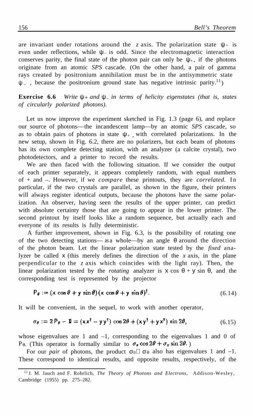
156 Bell’s Theorem
are invariant under rotations around the z axis. The polarization state ψ+ iseven under reflections, while ψ– is odd. Since the electromagnetic interactionconserves parity, the final state of the photon pair can only be ψ+, if the photonsoriginate from an atomic SPS cascade. (On the other hand, a pair of gammarays created by positronium annihilation must be in the antisymmetric stateψ – , because the positronium ground state has negative intrinsic parity.11)
Exercise 6.6 Write ψ+ and ψ– in terms of helicity eigenstates (that is, statesof circularly polarized photons).
Let us now improve the experiment sketched in Fig. 1.3 (page 6), and replaceour source of photons—the incandescent lamp—by an atomic SPS cascade, soas to obtain pairs of photons in state ψ+ , with correlated polarizations. In thenew setup, shown in Fig. 6.2, there are no polarizers, but each beam of photonshas its own complete detecting station, with an analyzer (a calcite crystal), twophotodetectors, and a printer to record the results.
We are then faced with the following situation. If we consider the outputof each printer separately, it appears completely random, with equal numbersof + and –. However, if we compare these printouts, they are correlated. I nparticular, if the two crystals are parallel, as shown in the figure, their printerswill always register identical outputs, because the photons have the same polar-ization. An observer, having seen the results of the upper printer, can predictwith absolute certainty those that are going to appear in the lower printer. Thesecond printout by itself looks like a random sequence, but actually each andeveryone of its results is fully deterministic.
A further improvement, shown in Fig. 6.3, is the possibility of rotating oneof the two detecting stations— a whole—by an angle θ around the directionas of the photon beam. Let the linear polarization state tested by the fixed ana-lyzer be called x (this merely defines the direction of the x axis, in the planeperpendicular to the z axis which coincides with the light ray). Then, thelinear polarization tested by the rotating analyzer is x cos θ + y sin θ, and thecorresponding test is represented by the projector
(6.14)
It will be convenient, in the sequel, to work with another operator,
(6.15)
whose eigenvalues are 1 and –1, corresponding to the eigenvalues 1 and 0 ofPθ. (This operator is formally similar to )
For our pair of photons, the product σ ⊗ σ0 θ also has eigenvalues 1 and –1.These correspond to identical results, and opposite results, respectively, of the
11 J. M. Jauch and F. Rohrlich, The Theory of Photons and Electrons, Addison-Wesley,Cambridge (1955) pp. 275–282.

Cryptodeterminism 157
Fig. 6.2. Photons originating in an SPS cascade, with opposite directions,have perfectly correlated linear polarizations. Here, there is a delay in thedetection of one of the photons, whose path is reflected by distant mirrors,far to the left (not shown). The lower detecting station is always activatedlater than the upper one, and its outcomes are predictable with certainty.
two analyzers. The average value of the observable σ0 ⊗ σ θ is the correlation ofthe outcomes of the two analyzers. Its value can be predicted by the standardrule for a quantum average, Eq. (3.41):
(6.16)
We obtain, as expected, a perfect correlation for θ = 0, a perfect anticorrelationfor θ = π /2, and Malus’s law for all the other angles.
Exercise 6.7 What is the correlation that has been measured in the exper-iment sketched in Fig. 6.3, until the last test recorded on that figure? Ans.:⟨ σ 0 ⊗ σ θ⟩ = 0.5.
Fig. 6.3. If one of the detecting stations is tilted byan angle θ, the correlation of the outcomes is cos 2θ .

158 Bell’s Theorem
Exercise 6.8 Show, from Eqs. (6.12) and (6.15), that if two analyzers testlinear polarizations at angles α and β from an arbitrary x axis, the correlationof their outcomes is
(6.17)
Bell’s model of hidden variables
The perfect correlation of distant and seemingly random events, illustratedin Fig. 6.2, suggests that the fundamental laws of physics are deterministic,and the apparent stochasticity of quantum phenomena is merely due to ourimperfect methods of preparing physical systems. Indeed, from the early daysof quantum theory, there were attempts to deduce its properties from those of adeterministic, yet unknown, subquantum world; and, on the other hand, therealso were numerous attempts to prove that no “hidden variable” theory couldreproduce the statistical properties of quantum theory.
In particular, von Neumann’s classic book12 contains a mathematical proofthat quantum theory is incompatible with the existence of “dispersion free en-sembles.” Namely, it is impossible to prepare an ensemble of physical systemsin such a way that every observable A satisfies ⟨ A² ⟩ = ⟨A⟩ ². The assumptionsneeded for von Neumann’s proof are that any observable A is represented by aself-adjoint operator (this is the essence of quantum theory); that if A and Bare observables, their sum A + B is also an observable; and moreover that
(6.18)
The last equation could be a trivial consequence of the trace formula (3.77), butvon Neumann does not want to use the trace formula in his proof—he ratherwants to derive it from weaker assumptions.
The difficulty, acknowledged by von Neumann himself, is that there is nophysical reason to assume the validity of Eq. (6.18), if the operators A and B donot commute and cannot be measured simultaneously. The three experimentalsetups needed for measuring A, B, and A + B, may be radically different (justthink of measuring the kinetic energy, or the potential energy, or the totalenergy of a physical system). One could therefore argue that a conventionalpreparation, which produces an ordinary quantum ensemble, satisfies (6.18),but more sophisticated preparation methods, not yet invented by us, couldcreate dispersion free ensembles, violating condition (6.18).
Following von Neumann’s questionable proof, there were other unsuccessfulattempts to derive the “no hidden variable theorem,” from different premises.All these efforts were finally laid to rest by Bell13 who explicitly constructed a
12 J. von Neumann, Mathematische Grundlagen der Quantenmechanik, Springer, Berlin(1932) p. 171; transl. by E. T. Beyer: Mathematical Foundations of Quantum Mechanics,Princeton Univ. Press, Princeton (1955) p. 324.
13J. S. Bell. Rev. Mod. Phys. 38 (1966) 447.

Cryptodeterminism 159
deterministic model, generating results whose averages were identical to thosepredicted by quantum theory.
–Bell’s model involves a spin1 particle and an observable A = m · σ, wherethe three components of m are arbitrary real numbers, and those of σ are
2
the Pauli spin matrices. According to quantum mechanics, a measurement ofA always yields one of its eigenvalues ±m (where m = m ) and the averageresult of an ensemble of measurements is . However, quantummechanics is unable to predict the specific outcome of each test. Bell’s modelassumes that this outcome is determined by m (a macroscopic parameter ofthe measuring apparatus, which we know to control), by ψ (the quantum statepreparation, which we can also control), and by an additional, hidden variablecalled λ. Conceptually, each physical system has a unique λ, but we are unableto know its value. Our present experimental techniques always end up yieldinga uniform distribution of λ, between –1 and 1. It is this uniform distributionwhich charaterizes the domain of validity of quantum theory. The model furtherspecifies that, for any given λ, the result of a measurement is:
— this occurs with probability
— this occurs with probability
Therefore the average result isin agreement with quantum mechanics.
Consider now another observable, B = n · σ , whose measurement yields ±n,according to the value of λ, by the same rule as for A. Furthermore, define athird observable, C = A + B = (m + n ) · σ. Notice that a measurement of Cwill always yield ± m + n ,and this result is not one of the four combinationsm+n, m–n, etc. Therefore, Eq. (6.18) cannot be valid for a particular value ofλ, nor in general for an arbitrary distribution of the values of λ . Nonetheless,Eq. (6.18) is valid for uniformly distributed λ, because, in that case, Bell’s modelguarantees agreement with quantum mechanics. We thus see that it is possibleto mimic all the statistical properties of quantum theory by a deterministichidden variable model.
In the same article,13 Bell also shows that this model can be extended tohigher dimensional Hilbert spaces; and then, he raises a new, cardinal question:If a quantum system consists of several disjoint subsystems, as in the EPRargument, will the hidden variables too fall into disjoint subsets? Bell showsthat his model does not satisfy this separability requirement, if the state of thequantum system is entangled:
. . . in this theory an explicit causal mechanism exists whereby the dispo-sition of one piece of apparatus affects the results obtained with a distantpiece. In fact the Einstein-Podolsky-Rosen paradox is resolved in the waywhich Einstein would have liked least.4
Finally, Bell asks whether it is possible to prove that “any hidden variableaccount of quantum mechanics must have this extraordinary character.” The

160 Bell’s Theorem
answer appears in a footnote, added at the end of this article: “Since thecompletion of this paper such a proof has been found.” (An editorial accidentcaused a two year delay in the publication of Bell’s article,13 which appearedlong after the proof mentioned at its end.14,15 That proof is Bell’s theorem onthe nonexistence of local hidden variables, discussed below.)
6-3 . Bell’s inequalities
The title of Bell’s second paper is “On the Einstein Podolsky Rosen paradox,”but, contrary to the EPR argument, Bell’s is not about quantum mechanics.Rather, it is a general proof, independent of any specific physical theory, thatthere is an upper limit to the correlation of distant events, if one just assumesthe validity of the principle of local causes. This principle (also called Einsteinlocality, but conjectured well before Einstein) asserts that events occurring ina given spacetime region are independent of external parameters that may becontrolled, at the same moment, by agents located in distant spacetime regions.Bell’s proof14 that the principle of local causes is incompatible with quantummechanics has momentous implications, and it was hailed as “the most profounddiscovery of science.”16
Here, you may object that the principle of local causes does not belong tophysics, but rather to philosophy, because it is of counterfactual nature. Theclaim that the occurrence of a particular event does not depend on some externalparameters implies a comparison between mutually exclusive scenarios, in whichthese external parameters have different values. For example, we may imaginethe existence of several replicas of the experiment of Fig. 6.3, with differentvalues of the angle θ, and we may reasonably claim that the results displayedby the upper printer should not depend on the tilt angle θ given to the lowerdetecting station. Bell’s theorem asserts that this claim—obvious as it mayappear—is incompatible with the cosine correlation law (6.17). As we shall see,that correlation is too strong.
Before discussing these quantum correlations, let us consider an elementaryclassical analog of the SPS photon cascade:1 7Imagine a bomb, initially at rest,which explodes into two asymmetric parts, carrying angular momenta J1 andJ 2 = –J1 . An observer detects the first fragment and measures the dynamicalvariable sign(α · J 1), where α is a unit vector with an arbitrary direction, chosenby that observer. The result of this measurement is called a and can only takethe values ±1. Likewise, a second observer detects the other fragment andmeasures sign(β · J 2 ), where β is another unit vector, chosen by the secondobserver. The result is b = ±1.
14 J. S. Bell, Physics 1 (1964) 195.15M. Jammer, Found. Phys. 20 (1990) 1139.16H. P. Stapp, Nuovo Cimento B 29 (1975) 270.17A. Peres, Am. J. Phys. 46 (1978) 745.

Bell’s inequalities 161
Fig. 6.4. A bomb, initially at rest, explodes into twofragments carrying opposite angular momenta.
This experiment is repeated N times. Let a j and b j be the results measuredby our observers for the jth bomb. If the directions of J 1 and J 2 are randomlydistributed, the averages obtained by each observer,
and (6.19)
are both close to zero (typically, they are of the order of 1/ ). However, ifthe observers compare their results, they find a correlation,
(6.20)
which, in general, does not vanish. For instance, if α = β, they always obtaina j = –bj , so that ⟨ ab⟩ = –1.
For arbitrary α and β, the expected correlation ⟨ ab⟩ can be computed asfollows: Consider a unit sphere, cut by an equatorial plane perpendicular toα, as shown in Fig. 6.5. We then have a = 1 if J 1 points through one of thehemispheres, and a = –1 if it points through the other hemisphere. Likewise,a second equatorial plane, perpendicular to β, determines the regions whereb = ±1. The unit sphere is thereby divided by these two equatorial planes intofour sectors, with alternating signs for the product ab. Adjacent sectors havetheir areas in the ratio of θ to π–θ, where θ is the angle between α and β .Thus, if J 1 is uniformly distributed, we obtain the classical correlation
(6.21)
Fig. 6.5. Geometric construction forobtaining the classical correlation(6.21). In the shaded areas, ab = 1;in the unshaded ones, ab = –1.

162 Bell’s Theorem
Let us now return to quantum mechanics. Consider two spin particles ina singlet state, far away from each other, like those of the Bohm model.5 Ourobservers measure the observables α · σ1 and β · σ 2 , where σ 1 and σ 2 are thePauli spin matrices pertaining to the two particles. The unit vectors α and βare freely chosen by the observers. As before, the results are called a and b, andcan have values ±1. Their mean values are predicted by quantum mechanics as⟨ a ⟩ = ⟨ b⟩ = 0, and their correlation as
(6.22)
In the singlet state, we have . Hence, with the help of the identity,we obtain
(6.23)
Figure 6.6 shows the expressions (6.20) and (6.23): the quantum correlationis always stronger than the classical one, except in the trivial cases where bothare 0 or ±1. Are you surprised? If so, this is the result of having been exposedto unfounded quantum superstitions, according to which quantum theory isafflicted by more “uncertainty” than classical mechanics. Exactly the oppositeis true: quantum phenomena are more disciplined than classical ones. We shallagain see this in Chapter 11, where quantum chaos will be found much tamerthan classical chaos.
Fig. 6.6. The quantumcorrelation (solid line)and the classical one(broken line) for a pairof spins, as functionsof the angle θ.
Bell’s theorem
Bell’s theorem is not a property of quantum theory. It applies to any physicalsystem with dichotomic variables, whose values are arbitrarily called 1 and –1.Its proof involves two distant observers and some counterfactual reasoning, justas in the EPR article.¹ However, while EPR merely pointed out a propertyof quantum theory which they found unsatisfactory, Bell derives quantitativecriteria for the existence of a realistic interpretation of any local theory.
The elementary algebraic proof below involves pairs of polarized photons,because this is the example most easily amenable to experimental verification.
–12

Bell’s inequalities 163
However, the result applies equally well to pairs of correlated spins, or indeedto any correlated systems, whether classical or quantal.
Consider a pair of photons, emitted in opposite directions in an SPS cascade.Two distant observers test their linear polarizations. The first observer has achoice between two different orientations of his polarization analyzer, makingangles α and γ with an arbitrary axis. For each orientation, his experiment hastwo possible (and unpredictable) outcomes. The hypothesis that we want totest is that the outcome which actually occurs is causally determined by localhidden variables, of unknown nature, but pertaining only to the photon andto the apparatus of the first observer. If he chooses angle α, that outcome iscalled α and may take values ±1. The measured observable thus is the onecalled σα in Eq. (6.15). Likewise, if the first observer chooses γ, he measuresσγ , and the same hidden variables determine the outcome c = ±1.
Einstein locality asserts that these outcomes cannot depend on parameterscontrolled by faraway agents. In particular, they do not depend on the orienta-tion of the analyzers used by the second observer. The latter also has a choiceof two alternative directions, β or γ (the same γ as may be chosen by the firstobserver). The outcomes of her test are b = ±1 or c = ±1, respectively, andare determined by the hidden variables of her photon and her apparatus.9
If both observers choose the same direction γ, they find the same result c, aswe already know. In any case, the results a, b, and c, identically satisfy
(6.24)
since both sides of this equation vanish if b = c, and are equal to ±2 if b ≠ c.Note that the various mathematical symbols in (6.24) refer to three tests, ofwhich any two, but only two, can actually be performed. At least one of thethree tests is counterfactual.
Suppose now that the same joint experiment is repeated many times, withmany consecutive photon pairs. Then, the three results (actual or imagined)for the j th photon pair satisfy
(6.25)
as in the preceding equation. Obviously, the hidden variables, which we do notcontrol, are different for each j. The serial number j can thus be understoodas a shorthand notation for the unknown values of these hidden variables. Inparticular, taking an average over the hidden variables is the same as taking anaverage over j, and therefore we have
a (b – c) ≡ ±(1 – b c),
(6.26)
Here, ⟨ ab⟩ is the sum of all the products a jbj , divided by the number of photonpairs. In other words, ⟨ ab⟩ is the correlation of the outcomes a and b. The result(6.26) is Bell’s inequality. (For perfectly anticorrelated pairs, as in Fig. 6.4, theright hand side of the inequality is 1 + ⟨ bc⟩ .)14
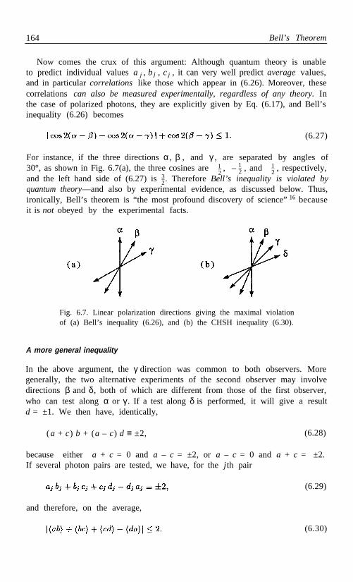
164 Bell’s Theorem
Now comes the crux of this argument: Although quantum theory is unableto predict individual values a j , b j , c j , it can very well predict average values,and in particular correlations like those which appear in (6.26). Moreover, thesecorrelations can also be measured experimentally, regardless of any theory. Inthe case of polarized photons, they are explicitly given by Eq. (6.17), and Bell’sinequality (6.26) becomes
(6.27)
For instance, if the three directions α , β , and γ , are separated by angles of30°, as shown in Fig. 6.7(a), the three cosines are , – , and , respectively,and the left hand side of (6.27) is3–2. Therefore Bell’s inequality is violated byquantum theory—and also by experimental evidence, as discussed below. Thus,ironically, Bell’s theorem is “the most profound discovery of science”16 becauseit is not obeyed by the experimental facts.
Fig. 6.7. Linear polarization directions giving the maximal violationof (a) Bell’s inequality (6.26), and (b) the CHSH inequality (6.30).
A more general inequality
In the above argument, the γ direction was common to both observers. Moregenerally, the two alternative experiments of the second observer may involvedirections β and δ, both of which are different from those of the first observer,who can test along α or γ. If a test along δ is performed, it will give a resultd = ±1. We then have, identically,
(a + c) b + (a – c) d ≡ ±2, (6.28)
because either a + c = 0 and a – c = ±2, or a – c = 0 and a + c = ±2.If several photon pairs are tested, we have, for the jth pair
(6.29)
and therefore, on the average,
(6.30)
–12
–12
–12
Bell’s inequalities 165
This result is called the CHSH inequality.18 Like Bell’s inequality (6.26), it isvalid for any set of dichotomic variables. It is an upper limit to the correlationof distant events, if the principle of local causes is valid. In the special case ofphotons with the correlation (6.17), this inequality becomes
(6.31)
For instance, if these various directions are separated by angles of 22.5°, asin Fig. 6.7(b), the first three cosines are 1/ , and the fourth one is –1Therefore the left hand side of (6.31) is 2 , which is obviously more than 2.We again reached a contradiction: there must be something wrong with ourphysical interpretation of the identity (6.30).
The theorem itself is not wrong, of course. It is based on Eq. (6.29), which istrivially true. The difficulty lies with the conceptual premises underlying thatidentity. Its physical interpretation is questionable and involves delicate pointsof logic, which will be discussed in the next section.
Exercise 6.9 Show that a linear correlation law, 1 – 2θ/ π, as in Eq. (6.21),satisfies both Bell’s inequality (6.26) and the CHSH inequality (6.30).
Exercise 6.10 Show that Bell’s inequality (6.26) is a special case of the CHSHinequality (6.30).
Exercise 6.11 Show that the maximal violation of Bell’s inequality (6.26)for polarized photons occurs when there are three angles of 30°, as in Fig. 6.7.Show likewise that the maximal violation of the CHSH inequality (6.30) occurswhen there are three angles of 22.5°.
Experimental tests
Physics is an experimental science, and theoretical predictions like Eqs. (6.26)and (6.30) must be tested in the laboratory. For correlated photons, this meansthat one must verify the cosine correlation (6.17), which was derived from thewave function ψ+ in Eq. (6.12), which was itself derived from purported sym-metry properties of atomic states and of their electromagnetic interaction. Forcorrelated fermions, it is the cosine correlation (6.23), illustrated in Fig. 6.6,which must be tested. These are difficult experiments, whose interpretation iscomplicated, because in real life one must take into account finite collimationangles and finite detector efficiencies.19
A static test like the one in Fig. 6.3, with fixed (or slowly moving) detectors,does not fully implement all the premises of Bell’s theorem. The latter involvetwo disjoint observers, who are free to choose their experiments out of mutuallyincompatible alternatives. These observers need not, of course, be humans: any
18J. F. Clauser, M. A .Horne, A Shimony, and R. A. Holt, Phys. Rev. Lett. 23 (1969) 880.19J. F. Clauser and A. Shimony, Rep. Prog. Phys. 41 (1978) 1881.

166 Bell’s Theorem
automatic devices, acting in a random fashion and independently of each other,effectively behave as these fictitious observers, endowed with free will.
An experiment20 simulating these conditions is sketched in Fig. 6.8. Thephotons, emitted by excited calcium atoms in SPS cascades, have wavelengthsλ1 = 422.7nm and λ 2 = 551.3 nm. (These photons are therefore distinguish-able, contrary to the situation in some more recent experiments21,22 which useparametric down conversion in nonlinear crystals.) Each photon that passesthrough a collimator (not shown in the figure) impinges on an acousto-opticalswitch, from where it is “randomly” directed toward one of two polarizationanalyzers. The two switches, which act like rapidly moving mirrors, are nottruly random, of course, but rather quasi-periodic. They are driven by differ-ent generators, at different frequencies, and it is plausible that they functionin uncorrelated ways. The distance between them is 12m, corresponding to asignal transit time of 40ns. This is much larger than the mean time betweenswitchings (about 10 ns), or the mean lifetime of the intermediate level of thecalcium atoms (5 ns). Therefore “the experimental settings are changed duringthe flight of the particles,” a feature that was deemed “crucial” by Bell.14
Fig. 6.8. Aspect’s experiment: Pairs of photons are emitted in SPS cascades.Optical switches O1 and O2 randomly redirect these photons toward four po-larization analyzers, symbolized by thick arrows. Each analyzer tests the linearpolarization along one of the directions indicated in Fig. 6.7(b). The detectoroutputs are checked for coincidences in order to find correlations between them.
This schematic description of Aspect’s experiment cannot do full justice tothis technical tour de force which took six years to be brought to completion.For the first time in the history of science, a physical process was controlledby two independent agents with a space-like separation, rather than a time-like one, as in every other experiment hitherto performed. The result was in
20A. Aspect, J. Dalibard, and G. Roger, Phys. Rev. Lett. 49 (1982) 1804.21 Y. H. Shih and C. O. Alley, Phys. Rev. Lett. 61 (1988) 2921.22J. G. Rarity and P.R. Tapster, Phys. Rev. Lett. 64 (1990) 2495.

Some fundamental issues 167
complete agreement with the quantum mechanical prediction, Eq. (6.17); andit violated the CHSH inequality (6.30) by five standard deviations.
6-4. Some fundamental issues
We must now find out what was wrong with the identity (6.29), which led usto conclusions inconsistent with experimental facts. There is no doubt thatcounterfactual reasoning is involved: the four numbers a j , b j , cj , dj , cannotbe simultaneously known. The first observer can measure either a j or c j , butnot both; the second one—either b j or d j . Therefore Eq. (6.29) involves at leasttwo numbers which do not correspond to any tangible data, and it cannot beexperimentally verified.
However, we do not normally demand that every number in every equationcorrespond to a tangible quantity. Counterexamples abound, even in classicalphysics (the vector potential A µ , the Hamilton-Jacobi function S, are two fa-miliar instances) Moreover, counterfactual reasoning is not illegitimate per se.It was endorsed by Bohr² in his answer to EPR; it is practiced daily, with noapparent ill effects, by people who ponder over a menu in a restaurant, or overan airline schedule in a travel agency. In the present case (correlated photonpairs) we can always imagine a table as the one below, including both actualand hypothetical results of performed and unperformed experiments. We lackthe information needed for filling the blanks in the last two rows of that table,but there are only 22N different ways of guessing the missing data cj and d j.Therefore, there are only 22 N different tables that can be imagined. The point isthat none of them obeys the cosine correlation (6.17). That correlation (whichhas been experimentally verified) is too strong to be compatible with Table 6-1.
Table 6-l. Actual and hypothetical outcomes of N quantum tests.
The tests were 1 2 3 4 5 6 . . . Nactually a j + + – + – – . . . +performed bj + – – + – – . . . +unperformed, c j ? ? ? ? ? ? . . . ?just imagined d j ? ? ? ? ? ? . . . ?
Let us see why a correlation which is too strong prevents the assignment ofconsistent values to c j and d j . Choose the various directions as in Fig. 6.7(b),so as to maximize the experimental violation of the CHSH inequality (6.30).Then, only a fraction sin² (π /8) 1/7 of the bj will not agree with the corre-sponding a j . Likewise, only 1/7 of the unknown c j will be different from b j , andonly 1/7 of the d j will differ from the corresponding c j . Thus, if we discard allthe j for which there is any disagreement among the outcomes of the above tests,we still remain with at least a fraction 1 – 3 sin² (π/8) 4/7 of the d j which

168 Bell’s Theorem
agree with the corresponding aj . On the other hand, the probability of agree-ment between a j and d j , predicted by Eq. (6.17), is only cos²(3π/8) 1/7.Therefore at least 3/7 (more precisely, – 10.4142) of the columns ofTable 6-l cannot be consistently filled. This conclusion can be succintly stated:unperformed experiments have no results.17
Exercise 6.12 Construct a similar table for the original Bell inequality (6.26).If the polarization tests are performed along the directions shown in Fig. 6.7(a),what fraction of the columns cannot be consistently filled? Ans.: 1/4.
Exercise 6.13 Show that a table like the above one is consistent with theweaker linear correlation 1 – 2θ/ π, which satisfies the CHSH inequality.
A 41% discrepancy, as in Table 6-1, is not a small effect, and calls for a fullinvestigation. Here is an exchange of opinions on this problem:23
Salviati. At the time of these measurements, the two observers are unawareof each other, e.g., they are mutually space-like. There is no possibility ofcommunication between them. It is therefore reasonable to assume, as EPRdid, that the actions of one observer do not influence the results of experimentsperformed by the other one. For example, the result a = 1 obtained by thefirst observer should not depend on whether the second one measures (or hasmeasured, or will measure) the photon polarization along β, or along δ.
Simplicio. This is obvious.
Sagredo. Your statement makes sense only if you assume that all theseevents are causally determined, even those which are unpredictable and seemto us random. Otherwise, you could not meaningfully compare the resultsthat are obtainable by the first observer under different and mutually exclusiveexternal conditions. I am seriously worried by this deterministic approach,because you have also assumed that the observers themselves have a free choiceamong the various experiments. Aren’t these observers physical systems too,and therefore subject to deterministic laws? Let us see how you solve thisapparent contradiction.
Salviati. Please, don’t detract me from my proof. The crucial point inBell’s argument is that although the individual results are unpredictable, theircorrelations, which are average values, can be computed by quantum theory, orcan simply be measured experimentally, irrespective of any theory. The amazingfact is that it is possible to prepare physical systems in such a way that theinequality (6.30) is violated, and therefore the identity (6.29) cannot be valid.
Simplicio. An identity which is not valid?
Salviati. This is of course impossible, therefore there must be a flaw in thisargument. Either it is wrong that the observers have a free choice among thealternative experiments (namely, for each pair of particles, only one of the fourexperimental setups is compatible with the laws of physics—the others are not,
23A. Peres, Found. Phys. 14 (1984) 1131.

Some fundamental issues 169
for reasons unknown to us), or it is wrong that each photon can be observedwithout disturbing the other photon. Take your choice.
Simplicio. Both alternatives are distasteful. I prefer classical physics.24
Salviati. I again insist: This difficulty is not the fault of quantum theory.Only experimental facts are involved here.20 So indeed we have a paradox.
Sagredo. There is a paradox only because you force on this physical systema description with two separate photons. These photons exist only in yourimagination. The only thing that you have really prepared is a pair of photons,in a spin zero state. That pair is a single, indivisible, nonlocal object. Now, ifyou like paradoxes, I can supply to you additional ones, at a greatly reduced costin labor and parts. You don’t have to invoke Einstein, Podolsky, and Rosen.You don’t need two photons. A single photon will do as well, in the standarddouble slit experiment. You just ask: How can the half-photon passing throughone of the slits know the position and shape of the other slit, through whichthe other half-photon is passing, so that it can interfere with it?
Simplicio. This question is meaningless! There are no half-photons. Aphoton is a single, indivisible, nonlocal object. This is why it can pass throughtwo widely separated slits and interfere with itself.
Salviati. A single photon can even originate from two different lasers.25 Wehave been since long familiar with nonlocal photons, electrons, etc.
Sagredo. And yet, you have no moral pangs in asking, in the EPR paradox,how can the first half of the pair (here) be influenced by the apparatus whichinteracts with the second half of the pair (there). After you know that eachparticle is stripped by quantum theory of all its classical attributes (it hasneither definite position, nor definite momentum, nor definite spin components),you still believe that it retains a well defined “existence,” as a separate entity.
Salviati.
Sagredo. The only paradoxical feature that I can see is that almost every-thing happens as if there were, at each instant, two distinct particles withreasonably well defined positions and momenta. It is only their polarizationstates that are inseparably entangled. That’s why you may be excused forhaving had no moral pangs, and EPR are excused too. But there is no paradox.
So, there is no paradox?
Nonlocality vs free will
In his opening statement, Sagredo admitted being worried by the fact that freewill had been granted to the two observers, in an otherwise deterministic world.Then, at the end of the dialogue, he opted for abandoning Einstein locality, andhe left the free will conundrum unsolved. As we shall now see, these two issuesare inseparably intertwined.
24G. Galileo, Discorsi e Dimostrazioni Matematiche, Intorno à Due Nuove Scienze, Elsevier,Leiden (1638).
25R . L. Pfleegor and L. Mandel, Ph7ys. Rev. 159 (1967) 1084.

170 Bell’s Theorem
Let us examine the consequences of nonlocality. Assume that the outcomea j, obtained by the first observer, depends on whether the second observerchooses to measure the polarization of her photon along β, or along δ. We shalldistinguish these two alternatives by means of more detailed notations, such asa j (β) and a j (δ) . If Einstein locality does not hold, these two numbers are notnecessarily equal. The left hand side of Eq. (6.29) then becomes
(6.32)
which can be 0, ±2, or ±4. The right hand side of the CSHS inequality (6.31)becomes 4, and there is no more any contradiction with experimental facts.
There seems to be, however, a new problem with potentially devastatingconsequences: Assuming that measurements are instantaneous (that is, verybrief), can we use these nonlocal effects to transfer information instantaneouslybetween distant observers ? For example, can the second observer find outthe orientation of the apparatus used by the first one? If this were possible,Einstein’s theory of relativity would be in jeopardy. In the present case, thereis no such danger, because, as long as the observers do not communicate andcompare their results, each one of them only sees a random sequence of + and –,carrying no information.
Exercise 6.14 Let ψ + , given by Eq. (6.12), represent the state of a pair ofcorrelated photons, and let be the corresponding density matrix.Show that if a partial trace is taken on the polarization states of one of thephotons, the other photon is described by a reduced density matrixwhich corresponds to a random polarization mixture.
Exercise 6.15 Show that if, contrary to postulate K (page 76), it were exper-imentally possible to distinguish a random mixture of photons with orthogonallinear polarizations from a random mixture of photons with opposite circularpolarizations, EPR correlations could be used for the instantaneous transferof information between arbitrarily distant observers (provided that these EPRcorrelations would be maintained for arbitrarily large distances).
The question may still be raised whether more sophisticated preparations ofcorrelated quantum systems would allow instantaneous transfer of information.Quantum theory by itself neither imposes nor precludes relativistic invariance.It only guarantees that if the dynamical laws are relativistically invariant (seeChapter 8), the particles used as information carriers cannot propagate fasterthan light over macroscopic distances—insofar as the macroscopic emitters anddetectors of these particles are themselves roughly localized.26 Therefore all thestatistical predictions (which are the only predictions) of relativistic quantumtheory necessarily satisfy Einstein locality.27
26A. Peres Ann. Phys. (NY) 37 (1966) 179.27More generally, one can define weak nonlocality, which cannot be used for information trans-
fer, and strong nonlocality, which could have such a use. For example, quantum correlationsare weakly nonlocal; the laws of rigid body motion are strongly nonlocal.

Some fundamental issues 171
On the other hand, a hidden variable theory which would predict individualevents must violate the canons of special relativity: there would be no covariantdistinction betweeen cause and effect. Yet, it is not inconceivable that a nonlocaland noncovariant hidden variable theory can be concocted in such a way that,after the hidden variables have been averaged out, the theory has only local andcovariant consequences. It must be so, indeed, if these average results coincidewith those predicted by relativistic quantum theory.
There is nothing unacceptable in the assumption that deterministic hiddenvariables underlie the statistical features of quantum theory. When Boltzmanncreated classical statistical mechanics, he assumed the existence of atoms, wellbefore anyone was able to observe—let alone manipulate—individual atoms.Boltzmann’s work was attacked by the school of “energeticists” who did not be-lieve in atoms, and wanted to base all of physical science on macroscopic energyconsiderations only. Later discoveries, relying on new experimental techniques,fully vindicated Boltzmann’s work.
One could likewise speculate that future discoveries will some day give usaccess to a subquantum world, described by these hypothetical hidden vari-ables which are purported to underlie quantum theory. It is here that Bell’stheorem comes to put a cap on science fiction. In a completely deterministictheory, which would necessarily be nonlocal, separate parts of the world wouldbe deeply and conspiratorially entangled, and our apparent free will would beentangled with them.28 (If you hesitate to include “free will” in the theory,you may replace the human observers by automatons, having random and un-correlated behaviors. Just imagine two telescopes pointing toward differentdirections in the sky and counting whether an odd or even number of photonsarrive in a predetermined time interval.) A reasonable compromise thus is toabandon Einstein locality for individual phenomena, which are fundamentallyunpredictable, but to retain it for quantum averages, which can be predictedand causally controlled.
However, once we accept this attitude, doubts about the existence of “freewill” appear again: Why can’t our pair of observers be considered as a single,indivisible, nonlocal entity? Their past histories are undeniably correlated, sincethey agreed to collaborate in a joint experiment. Consider the similar, but muchsimpler issue illustrated in Fig. 6.2, where two photons have correlated histories.Each one of the two records appears “random” (each apparatus seems to have“free will”) if we disregard the information in the other record. The latter iscrucial, because the photon pair is a single, indivisible, nonlocal object. If weignore the correlation, every outcome looks random. Likewise, when people areconsidered individually, and their past interactions with other people or thingsare ignored, they appear to behave randomly—to have “free will.”29
Can unknown correlations restrict our apparent free will? A similar questionalso bears on the experiment in Fig. 6.2, in which randomness is not completely
28J. S. Bell, J. Physique 42 (1981) C2-41.29A. Peres, Found. Phys. 16 (1986) 573.

172 Bell’s Theorem
eliminated: we can predict the second sequence after seeing the first one, butwe cannot predict the first one. Can the remaining randomness be reducedby finding further correlations? This would require to trace back the historiesof the atoms that emitted the SPS cascades. If the latter were produced bya coherent process, it may be possible to correlate these photon pairs withother observable phenomena. On the other hand, if the excitation process wasthermal, further correlations are practically lost. Turning now our attentionto considerably more complex systems, such as human beings, it is obviousthat any EPR correlation between them is swamped by myriads of irreversibleprocesses. The result is that each one of us behaves unpredictably, as if endowedwith free will; this is why the expression “each one” can be used when we talkabout people like you and me.
In our daily work as physicists, we are compelled to use only incompleteinformation on the world, because we cannot know everything. The methodthat we use in physics is the following. We divide the world into three parts,which are the system under study, the observer (or the observing apparatus),and the rest of the world (that is, most of it!) which, we pretend, is unaffectedby the two other parts. We further assume that, if the system under observationis sufficiently small, it can be perfectly isolated from everything else,30 exceptfrom the observer testing it, if and when it is tested. This makes things appearsimple. This method is what gives to physics the aura of an exact science.For example, we can compute the properties of the hydrogen atom to umpteendecimal places, because when we do these calculations, there is nothing but asingle hydrogen atom in our conceptual world.
We work as if the world could be dissected into small independent pieces.This is an illusion. The entire world is interdependent. We see that in everyexperiment where Bell’s inequality is violated. But we have no other way ofworking. The practical questions with which we are faced always are of thetype: Given a finite amount of information, what are the possible outcomes ofthe ill-defined experiments that we prepare? The answers must necessarily beprobabilistic, by the very nature of the problem.
Is quantum theory universally valid?
The proof of Bell’s theorem requires the observed system to be deterministic,while the observers are not. If observers enjoy the privilege of immunity from thelaws of a deterministic theory, we still have a logically consistent scheme, but itis not a universal one. (By way of analogy: celestial mechanics is deterministicand puts no restrictions on our ability to measure the positions of planets andasteroids, but celestial mechanics does not explain the functioning of telescopes
3 0More precisely, a microscopic system can be isolated from any unknown effects originating inthe rest of the world. That system may still interacts with a perfectly controlled environment,such as an external magnetic field, which is then treated as a known term in the system’sHamiltonian.
Other quantum inequalities 173
and photographic plates, nor was it intended to.)31
On the other hand, we believe that our apparatuses are made of atoms andthat their macroscopic behavior is reducible to that of their elementary con-stituents. There is nothing in quantum theory making it applicable to threeatoms and inapplicable to 1023. At this point, it is customary to argue thatobservers (or measuring apparatuses) are essentially different from microscopicphysical objects, such as molecules, because they are very big, and therefore it isimpossible to isolate them from unknown and uncontrollable effects originatingin the rest of the world. They are open systems. However, the mental boundarybetween our ideal quantum world and tangible reality is arbitrary and fuzzy,just like the boundary between reversible microscopic systems and irreversiblemacroscopic ones. I shall return to this problem at the end of the book.
Even if quantum theory is universal, it is not closed. A distinction must bemade between endophysical systems—those which are described by the theory—and exophysical ones, which lie outside the domain of the theory (for example,the telescopes and photographic plates used by astronomers for verifying thelaws of celestial mechanics). While quantum theory can in principle describeanything, a quantum description cannot include everything. In every physicalsituation something must remain unanalyzed. This is not a flaw of quantumtheory, but a logical necessity in a theory which is self-referential and describesits own means of verification.31 This situation reminds of Gödel’s undecidabilitytheorem:32 the consistency of a system of axioms cannot be verified becausethere are mathematical statements that can neither be proved nor disprovedby the formal rules of the theory; but they may nonetheless be verified bymetamathematical reasoning.
In summary, there is no escape from nonlocality. The experimental violationof Bell’s inequality leaves only two logical possibilities: either some simplephysical systems (such as correlated photon pairs) are essentially nonlocal, orit is forbidden to consider simultaneously the possible outcomes of mutuallyexclusive experiments, even though any one of these experiments is actuallyrealizable. The second alternative effectively rules out the introduction of exo-physical automatons with a random behavior—let alone observers endowed withfree will. If you are willing to accept that option, then it is the entire universewhich is an indivisible, nonlocal entity.
6-5. Other quantum inequalities
The stunning implications of Bell’s theorem caused an outbreak of theoreticalactivity, including wild speculations that I shall not discuss. On the seriousside, Bell’s work led to a systematic search for other universal inequalities.
31A. Peres and W. H. Zurek, Am. J. Phys. 50 (1982) 807.32K. Gödel, Monat. Math. Phys. 38 (1931) 173 [transl.: On Formally Undecidable Proposi-
tions of Principia Mathematica and Related Systems, Basic Books, New York (1962)].
174 Bell’s Theorem
Cirel'son's inequality
Cirel’son33 raised the question whether quantum theory imposed an upper limitto correlations between distant events (a limit which would of course be higherthan the classical one, given by Bell’s inequality).
Let us consider four operators, σ α , σβ , σ γ, and σδ, with algebraic propertiessimilar to those of the observables in the Aspect experiment (Fig. 6.8). Theseoperators satisfy and
(6.33)
Define an operator
(6.34)
with the same structure as the combination which appears on the left hand sideof the CHSH inequality (6.30). We have identically34
(6.35)
The identities (4.27), page 86, give, for any two bounded operators A and B,
(6.36)
and therefore, in the present case, andfollows from Eq. (6.35) that or
It thus
This is Cirel’son’s inequality. Its right hand side is exactly equal to the upperlimit that can be attained by the left hand side of the CHSH inequality (6.30).Quantum theory does not allow any stronger violation of the CHSH inequalitythan the one already achieved in Aspect’s experiment.
Further insight in this problem can be gained by choosing a basis which makesboth [σα , σ γ] and [σβ , σδ] diagonal, with eigenvalues λn and Λµ , respectively.35
In that basis, C ² is also diagonal, with eigenvalues 4 + λn Λµ . If it happensthat all the λ n (or all the Λ µ ) vanish, we have ||C || = 2 exactly, and thereis no disagreement with the CHSH inequality (6.30). None should indeed beexpected, since at least one of the observers is not involved with incompatibletests. However, in general, there are nonvanishing eigenvalues λn and Λ µ . Ifthere is a pair for which λn, Λ µ > 0, the corresponding eigenvectors representa state which violates the CHSH inequality, becauseIt can be shown35 that these violations come with both signs: if ξ > 2 is aneigenvalue of C, then –ξ also is an eigenvalue of C.
(6.37)
33B. S. Cirel’son, Lett. Math. Phys. 4 (1980) 93.34L. J. Landau, Phys. Letters A 120 (1987) 54.35S. L. Braunstein, A. Mann, and M. Revzen, Phys. Rev. Lett. 68 (1992) 3259.
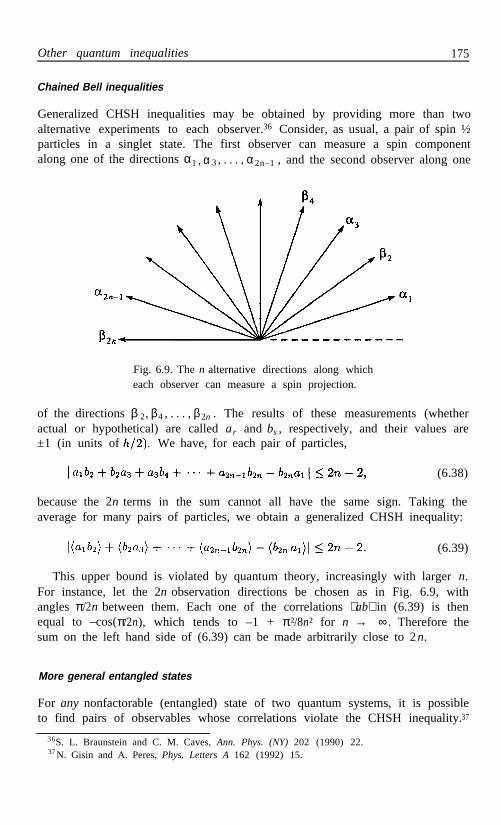
Other quantum inequalities 175
Chained Bell inequalities
Generalized CHSH inequalities may be obtained by providing more than twoalternative experiments to each observer.36 Consider, as usual, a pair of spin ½particles in a singlet state. The first observer can measure a spin componentalong one of the directions α1 , α 3, . . . , α 2n–1 , and the second observer along one
Fig. 6.9. The n alternative directions along whicheach observer can measure a spin projection.
of the directions β 2, β4 , . . . , β2n . The results of these measurements (whetheractual or hypothetical) are called ar and bs , respectively, and their values are±1 (in units of We have, for each pair of particles,
(6.38)
because the 2n terms in the sum cannot all have the same sign. Taking theaverage for many pairs of particles, we obtain a generalized CHSH inequality:
(6.39)
This upper bound is violated by quantum theory, increasingly with larger n.For instance, let the 2n observation directions be chosen as in Fig. 6.9, withangles π/2n between them. Each one of the correlations ⟨ ab⟩ in (6.39) is thenequal to –cos(π/2n), which tends to –1 + π²/8n² for n → ∞. Therefore thesum on the left hand side of (6.39) can be made arbitrarily close to 2n.
More general entangled states
For any nonfactorable (entangled) state of two quantum systems, it is possibleto find pairs of observables whose correlations violate the CHSH inequality.37
36S. L. Braunstein and C. M. Caves, Ann. Phys. (NY) 202 (1990) 22.37N. Gisin and A. Peres, Phys. Letters A 162 (1992) 15.

176 Bell’s Theorem
Indeed, any ψ ∈ H 1 ⊗ H 2 can be written as a Schmidt bi-orthogonal sumwhere ui and vi are orthonormal bases in H 1 and H 2,
respectively. It is possible to choose their phases so that all the ci are real andnon-negative, and to label them so that c1 ≥ c2≥ ··· ≥ 0. We shall now restrictour attention to the N -dimensional subspaces of H1 and H 2 which correspondto nonvanishing c j . A nonfactorable state is one for which N > 1.
With orthonormal bases defined as above, let Γx and Γ z be block-diagonalmatrices, where each block is an ordinary Pauli matrix, σ x and σ z , respectively:
(6.40)
If N is odd—which slightly complicates the proof—we take (Γ z ) N N = 0, andwe define still another matrix, Π, whose only nonvanishing element is Π N N = 1.If N is even, Π is the null matrix. It is also convenient to define a number γ by
(odd N ) and γ : = 0 (even N ). (6.41)
With the above notations, consider the observables
(6.42)
The eigenvalues of A(α ) and B (β ), denoted by a and b respectively, are ±1,and the correlation of these observables is
(6.43)
where
(6.44)
is always positive for a nonfactorable state. In particular, if we choose α = 0,α ’ = π/2 , and β = – β’ = tan–1[ K /(1 – γ)], we obtain
(6.45)
(6.46)
which contradicts the CHSH inequality (6.30).
Exercise 6.16 Verify Eqs. (6.43) and (6.45).
Exercise 6.17 Prove that γ ≥ 1/N and γ < 1 – K .
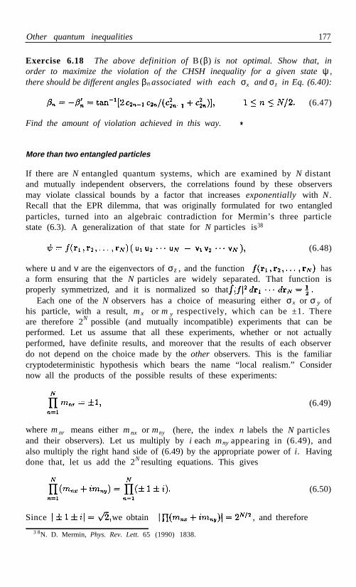
Other quantum inequalities 177
Exercise 6.18 The above definition of B(β) is not optimal. Show that, inorder to maximize the violation of the CHSH inequality for a given state ψ ,there should be different angles βn associated with each σx and σz in Eq. (6.40):
Find the amount of violation achieved in this way.
If there are N entangled quantum systems, which are examined by N distantand mutually independent observers, the correlations found by these observersmay violate classical bounds by a factor that increases exponentially with N.Recall that the EPR dilemma, that was originally formulated for two entangledparticles, turned into an algebraic contradiction for Mermin’s three particlestate (6.3). A generalization of that state for N particles is38
where u and v are the eigenvectors of σz , and the function hasa form ensuring that the N particles are widely separated. That function isproperly symmetrized, and it is normalized so that
Each one of the N observers has a choice of measuring either σx or σ y ofhis particle, with a result, m x or m y respectively, which can be ±1. Thereare therefore 2N possible (and mutually incompatible) experiments that can beperformed. Let us assume that all these experiments, whether or not actuallyperformed, have definite results, and moreover that the results of each observerdo not depend on the choice made by the other observers. This is the familiarcryptodeterministic hypothesis which bears the name “local realism.” Considernow all the products of the possible results of these experiments:
where m nr means either m nx or mny (here, the index n labels the N particlesand their observers). Let us multiply by i each mny appearing in (6.49), andalso multiply the right hand side of (6.49) by the appropriate power of i. Havingdone that, let us add the 2N resulting equations. This gives
Since we obtain , and therefore
3 8N. D. Mermin, Phys. Rev. Lett. 65 (1990) 1838.
(6.47)
(6.48)
(6.49)
(6.50)
More than two entangled particles
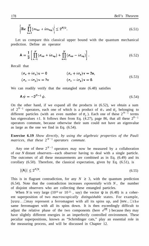
178 Bell’s Theorem
(6.51)
Let us compare this classical upper bound with the quantum mechanicalprediction. Define an operator
Recall that
We can readily verify that the entangled state (6.48) satisfies
On the other hand, if we expand all the products in (6.52), we obtain a sumof 2N –1 operators, each one of which is a product of σ x and σy belonging todifferent particles (with an even number ofσy ). Each one of these 2N– 1 terms
N– 1
operators commute, because otherwise their sum could not have an eigenvalueas large as the one we find in Eq. (6.54).
Exercise 6.19 Show directly, by using the algebraic properties of the Paulimatrices, that these 2N –1 operators commute.
Any one of these 2N –1 operators may now be measured by a collaborationof our N distant observers—each observer having to deal with a single particle.The outcomes of all these measurements are combined as in Eq. (6.49) and itscorollary (6.50). Therefore, the classical expectation, given by Eq. (6.51), is
This is in flagrant contradiction, for any N ≥ 3, with the quantum prediction(6.54). Note that the contradiction increases exponentially with N , the numberof disjoint observers who are collecting these entangled particles.
When N is very large (1010 or 1025 , say) the vector ψ in (6.48) is a coher-ent superposition of two macroscopically distinguishable states. For example,|uuu. . .⟩ may represent a ferromagnet with all its spins up, and |vvv... ⟩ t h esame ferromagnet with all its spins down. It is then exceedingly difficult toadjust the relative phase of the two components (here eiπ ) because they mayhave slightly different energies in an imperfectly controlled environment. Thesepeculiar superpositions, known as “Schrödinger cats,” play an essential role inthe measuring process, and will be discussed in Chapter 12.
(6.55)
(6.53)
(6.54)
(6.52)
has eigenvalues ±1. It follows then from Eq. (4.27), page 86, that all these 2

Higher spins 179
6-6. Higher spins
It is commonly believed that classical properties emerge in the limit of largequantum numbers. Let us examine whether there is a smooth transition fromquantum theory to classical physics. Consider a pair of spin j particles witharbitrarily large j, prepared in a singlet state as usual (rather than spinparticles as we considered until now, or polarization componenents of photonswhich have similar algebraic properties).
The EPR argument is applicable to our spin j particles, exactly as before.Separate measurements of J l z and J2z by two independent observers must giveopposite values, since the value of J1z + J 2 z is zero. More generally, we areinterested in the correlation of the results of measurements of J1 and J 2 alongnon-parallel directions, arbitrarily chosen by the two observers.
We shall need the explicit form of the vector ψ 0 that represents two spin jparticles with total angular momentum zero. For each particle, we have
where and = 1 for simplicity. In order to satisfythe singlet state must have the form
This is a Schmidt bi-orthogonal sum, as in Eq. (5.31). Therefore, the datathat can be obtained separately by each observer are given by identical densitymatrices ρ, which are diagonal, with elements |cm |² summing up to 1.
Moreover, all the probabilities |cm|² are equal. The reason simply is thata zero angular momentum state is spherically symmetric, and the z-axis hasno special status. Any other polar axis would yield the same diagonal densitymatrix ρ, with the same elements |cm |². As the choice of another axis is a mererotation of the coordinates, represented in quantum mechanics by a unitarytransformation, ρ → UρU† , it follows that ρ commutes with all the rotationmatrices U. Now, for any given j , these matrices are irreducible.39 Therefore ρis a multiple of the unit matrix, and |cm |² = (2j + 1)–1 . Only the phase of c m
remains arbitrary (because those of um and vm are).
Exercise 6.20 Show that
Exercise 6.21 Show that for the singlet state ψ0 , and for half-integral j,Eq. (6.44) gives K = 1, causing the maximal violation of the CHSH inequalityallowed by Cirel’son’s theorem. What happens for integral j ?
Exercise 6.22 Show that the standard choice for the matrices Jx (symmetricand real) and J y (antisymmetric and pure imaginary) gives
This result generalizes Eq. (5.33), which was valid for spin .
3 9E. P. Wigner, Group Theory, Academic Press, New York (1959) p. 155.
and (6.56)
(6.57)

180 Bell’s Theorem
Consider now the following experiment: The two spin j particles, prepared inthe singlet state (6.57), fly apart along the ±x directions (collimators eliminatethose going toward other directions). The two distant observers apply to eachparticle that they collect a torque around its direction of motion, for exampleby letting the particles pass through solenoids, where each observer can controlthe magnetic field. The state of the pair thus becomes
The last step follows from which holds for a singlet state.Each observer then performs a Stern-Gerlach experiment, to measure J 1z
and J 2 z , respectively. There is no fundamental limitation to the number ofdetectors involved in such an experiment (2j + 1 = 10
9detectors, say) because
it is always possible, at least in principle, to position the detectors so far awayfrom the Stern-Gerlach magnets that the 2j + 1 beams are well separated, andthe corresponding m can be precisely known. (An equivalent experiment wouldbe to apply no torque, and to rotate the Stern-Gerlach magnets, together withall their detectors, by angles θ1and θ 2 .)
Notice that a Stern-Gerlach experiment measures not only Jz, but also anyfunction as defined by Eq. (3.58), page 68. In partic-ular, a Stern-Gerlach experiment measures the dichotomic variable,
which has eigenvalues ±1. The correlation of the values obtained by the twoobservers for these dichotomic variables is the mean value of their product:
(6.60)
where θ = θ1 – θ2, for brevity. Note that and commute; that(because ψ0 is a singlet state); and that generates
a rotation by an angle π around the z -axis, so that
(6.61)
We thus obtain
(6.62)
where the last step used rotational invariance. Together with (6.57), this gives
This sum is an ordinary geometric series, and we finally have
(6.58)
(6.59)
(6.63)

Higher spins 181
(6.64)
We can now apply the CHSH inequality (6.30) in the usual way: If the firstobserver has a choice between parameters θ1 and θ3, and the second observerbetween θ2 and θ4 , that inequality becomes:
Let us take When j → ∞, the lefthand side of (6.65) tends to a constant, whose maximum value is obtained forx = 1.054:
It is possible to obtain an even stronger violation, up to which is themaximum allowed by Cirel’son’s inequality (6.37), by using particles having anelectric quadrupole moment besides their magnetic dipole moment.37
In summary, if the resolution of our instruments is sharp enough for dis-criminating between consecutive values of m, their readings violate the CHSHinequality, and therefore invalidate its classical premises. The conclusion is thatmeasurements which resolve consecutive values of m are inherently nonclassical.No matter how large j may be, there is no reason to expect the results of theseideal measurements to mimic classical behavior.40
Exercise 6.23 Generalize the preceding calculations to the case where thetorques are applied around axes that are not parallel.
Observations in a noisy environment
There is a serious practical difficulty in the ideal experiment that was justdescribed. The dissemination of all these spin j particles among a multitudeof detectors, unless accompanied by a proportional increase of the incomingbeam intensity, reduces the statistical significance of the results and makes themhighly sensitive to noise. In particular, a compromise must be sought betweendetection failures and false alarms. As the detectors are mutually independent,there are no correlations between the wrong signals that they generate, andthe noise has a white spectrum.41 This means that if we carry out a discreteFourier transform from the variable m, which labels the outgoing beams, toa frequency-like variable, the power spectrum of the noise is uniform for allfrequencies. This situation is familiar in communications engineering. The keyto noise reduction is a suitable filtering which retains only the low frequencypart of the spectrum.41
In our example, this filtering can be done as follows. First, we note that, inthe absence of noise, the probability amplitude for the pair of results m 1 andm2 is given by Eqs. (6.57) and (6.58) as
40 N. D. Mermin and G. M. Schwarz, Found. Phys. 12 (1982) 101.41 J. R. Pierce, An Introduction to Information Theory: Symbols, Signals and Noise, Dover,
New York (1980).
(6.65)
(6.66)

182 Bell’s Theorem
(6.67)
Therefore the joint probability for the results m1 and m 2 is
A discrete Fourier transform, from m 1 and m 2 to the frequency-like variables ξand η , gives
where the last inner product was obtained thanks to the definition of the adjointof an operator—see Eq. (4.28). The double sum in (6.70) can be rearranged as
To evaluate this trace, we note that each one of the exponents on the righthand side of (6.71) is a rotation operator, and therefore their product also isa rotation operator, by some angle κ that we have to determine. The crucialpoint here is that κ is a function of the separate rotation angles, ξ , η , and± θ , but not of the spin magnitude j (the latter affects only the order of therotation matrices, not their geometrical meaning). In order to compute κ , wemay simply pretend that j = , so as to handle nothing bigger than 2 by 2matrices. Moreover, we actually need only the absolute value of κ , not thedirection of the combined rotation axis. It is easily found that
Exercise 6.24 Verify Eq. (6.72) and show that it can also be written as
Exercise 6.25 Find the direction of the vector κ (the rotation axis).
We can now evaluate the trace in (6.71). As a trace is independent of thebasis used in Hilbert space, it is convenient to take the basis that diagonalizesκ ·J, whose eigenvalues areκ j, κ( j – 1), . . . , –κ j . We obtain
(6.68)
(6.69)
(6.70)
(6.71)
(6.72)
(6.73)
12–
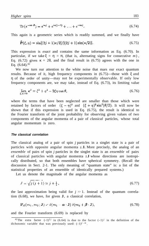
Higher spins 183
(6.74)
This again is a geometric series which is readily summed, and we finally have
(6.75)
This expression is exact and contains the same information as Eq. (6.70). Inparticular, if we takeξ = η = π, (that is, alternating signs for consecutive m ) ,Eq. (6.72) gives κ = 2θ, and the final result in (6.75) agrees with the one inEq. (6.64).42
We now turn our attention to the white noise that mars our exact quantumresults. Because of it, high frequency components in (6.75)—those with ξ andη of the order of unity—may not be experimentally observable. If only lowfrequency components are, we may take, instead of Eq. (6.73), its limiting value
(6.76)
where the terms that have been neglected are smaller than those which wereretained by factors of order and It will now beshown that if this expression is used in Eq. (6.75), the result is identical tothe Fourier transform of the joint probability for observing given values of twocomponents of the angular momenta of a pair of classical particles, whose totalangular momentum is zero.
The classical correlation
The classical analog of a pair of spin j particles in a singlet state is a pair ofparticles with opposite angular momenta± J. More precisely, the analog of anensemble of pairs of spin j particles in the singlet state is an ensemble of pairsof classical particles with angular momenta ±J whose directions are isotropi-cally distributed, so that both ensembles have spherical symmetry. (Recall thediscussion in Sect. 2-1. The only meaning of “quantum state” is: a list of thestatistical properties of an ensemble of identically prepared systems.)
Let us denote the magnitude of the angular momenta as
(6.77)
the last approximation being valid for j >> 1. Instead of the quantum correla-tion (6.68), we have, for given J , a classical correlation,
(6.78)
and the Fourier transform (6.69) is replaced by
42The extra factor (–1)2 j in (6.64) is due to the factor (–1)j in the definition of thedichotomic variable that was previously used: (–1)j – m .

184 Bell’s Theorem
(6.79)
(6.80)
where
This classical correlation must now be averaged over all possible directionsof J. As the latter are isotropically distributed, we have
(6.81)
where d Ω is the infinitesimal solid angle element in the direction of J. To performthe integration, let us take the direction of k as the polar axis, so that
J · k = J k u, (6.82)
(6.83)
where
and where u is the cosine of the angle between J and k. We can then takedΩ = 2π du by virtue of the rotational symmetry of eiJ· k around the directionof k, and Eq. (6.81) becomes
Since α ·β = cosθ (where θ has the same meaning as before) we find that
is exactly the same as the limiting value of κ in Eq. (6.76). We thus finallyhave, for large j and small k ,
(6.84)
(6.85)
(6.86)
in complete agreement with the limiting value of the quantum correlationin Eq. (6.75), for large j and small κ .
How coarse should our instruments be, in order to obtain this agreement ofclassical and quantum results? We have seen, in the derivation of Eq. (6.76),that the error made in approximating κ by its limiting value k is of the order of
and This error is then multiplied by j, in Eq. (6.75).Therefore will be well approximated by if both and
hold. In other words, the noise level must be such thatthe only detectable “frequencies” ξ and η are those for which both and
are much smaller than j –1/2. This high frequency cutoff implies

Bibliography 185
that different values of m can be experimentally distinguished only if they areseparated by much more than
This result had to be expected on intuitive grounds: In order to reduce thequantum correlation to a value similar to that of the weaker classical correlation,the minimum amount of blurring that one needs is obviously larger than theintrinsic “uncertainty” imposed by quantum mechanics on the components ofthe angular momentum vector. The latter is ( t h i swill be proved in Sect. 10-7). The minimum uncertainty is achieved by angularmomentum coherent states that satisfy n · J ψ = j ψ, for some unit vector n .For example the state uj , defined by J z u j = juz , gives
(6.87)
whence This is the minimal angular dispersion compatiblewith quantum mechanics. If the angular resolution of our instruments is muchpoorer than this limit, they cannot detect the effects of quantum nonlocality.
6-7. Bibliography
Collections of reprints
J. S. Bell, Speakable and Unspeakable in Quantum Mechanics, CambridgeUniv. Press (1987).
This is a complete anthology of John Bell’s published and unpublished articles onthe conceptual and philosophical problems of quantum mechanics.
L. E. Ballentine, editor, Foundations of Quantum Mechanics Since the BellInequalities, Amer. Assoc. Phys. Teachers, College Park (1988).
This book lists 140 recent articles on the foundations of quantum theory, with briefcomments on each one. Fifteen of these articles are also reprinted.
N. D. Mermin, Boojums All the Way Through: Communicating Science ina Prosaic Age, Cambridge Univ. Press (1990).
This is a collection of essays in which David Mermin’s wry humor is combined withhis commitment to finding simple ways of presenting complex ideas. The book includesvarious ways of demonstrating the extraordinary implications of Bell’s theorem, as wellas amusing anecdotes, such as the adventures that befell the author when he introducedthe word “boojum” into the technical lexicon of modern physics.
Conference proceedings
J. T. Cushing and E. McMullin, eds., Philosophical Consequences of Quan-tum Theory: Reflections on Bell’s Theorem, Univ. of Notre Dame Press (1989).
M. Kafatos, editor, Bell’s Theorem, Quantum Theory, and Conceptions ofthe Universe, Kluwer, Dordrecht (1989).
and

186 Bell’s Theorem
Kurt Gödel’s revolutionary paper32 challenged basic assumptions of mathematicallogic. Two nontechnical accounts of Gödel’s theorem are:
E. Nagel and J. R. Newman, Gödel’s Proof, New York Univ. Press (1958).
D. R. Hofstadter, Gödel, Escher, Bach: an Eternal Golden Braid, BasicBooks, New York (1979).
The latter book won the 1980 Pulitzer Prize for general non-fiction. The author’sremarkable achievement is the use of a entertaining style to make one of the mostabstract ideas of mathematical logic understandable by the general reader.
G. J. Chaitin, “Gödel’s theorem and information,” Int. J. Theor. Phys. 21(1982) 941.
Gödel’s theorem is demonstrated by arguments with an information-theoretic flavor:if a theorem contains more information than a set of axioms, that theorem cannotbe derived from these axioms. This suggests that the incompleteness phenomenondiscovered by Gödel’s is natural and widespread, rather than pathological and unusual.
N. Herbert, Quantum Reality, Anchor Press-Doubleday, New York (1985).
Herbert’s book is a well illustrated narrative of Bell’s discovery and its implications.
A. Garg and N. D. Mermin, “Bell’s inequalities with a range of violation thatdoes not diminish as the spin becomes arbitrary large,” Phys. Rev. Lett. 49(1982) 901, 1294 (E).
Garg and Mermin were the first to show that spin j particles in a singlet state havecorrelations which violate Bell’s inequality for measurements along nearly all directions.However, the magnitude of the violation that they found vanished exponentially forlarge j because of the use of slowly varying functions of the spin components, whichmade their method insensitive to the rapidly varying part of the quantum correlations.
W. De Baere, “Einstein-Podolsky-Rosen paradox and Bell’s inequalities,”Adv. Electronics and Electron Physics, 68 (1986) 245.
D. M. Greenberger, M. A. Horne, A. Shimony, and A. Zeilinger, “Bell’stheorem without inequalities,” Am. J. Phys. 58 (1990) 1131.
L. Hardy, “Nonlocality for two particles without inequalities for almost allentangled states,” Phys. Rev. Lett. 71 (1993) 1665; “Nonlocality of a singlephoton revisited,” ibid. 73 (1994) 2279.
Hardy derives two surprising results: states that are not maximally entangled maygive stronger effects; and a single particle is enough to violate Einstein causality.
A. Peres, “Nonlocal effects in Fock space,” Phys. Rev. Lett. (1995) in press.
Gödel’s theorem
Recommended reading
Recent progress, curiouser and curiouser

Chapter 7
Contextuality
7-1. Nonlocality versus contextuality
In the preceding chapter, it was shown that, for any nonfactorable quantumstate, it is possible to find pairs of observables whose correlations violate Bell’sinequality (see page 176). This means that, for such a state, quantum theorymakes statistical predictions which are incompatible with the demand that theoutcomes of experiments performed at a given location in space be independentof the arbitrary choice of other experiments that can be performed, simultane-ously, at distant locations (this apparently reasonable demand is the principleof local causes, also called Einstein locality) .
However, it is not easy to demonstrate experimentally a violation of Bell’sinequality. The predicted departure from classical realism appears only at thestatistical level. Even formulations of Bell’s theorem “without inequalities”cannot be verified by a single event. Therefore, any purported experimentalverification is subject to all the vagaries of nonideal quantum detectors.
In the present chapter, we shall encounter another class of “paradoxes” whichresult from counterfactual logic. These new contradictions between quantumtheory and cryptodeterminism do not depend on the choice of a particularquantum state, and therefore they are free from statistical inferences. Operatoralgebra is the only mathematical tool which is required. On the other hand,postulates stronger than the principle of local causes are needed.
Degeneracy and compatible measurements
If a matrix A is not degenerate, there is only one basis in which A is diagonal.That basis corresponds to a maximal quantum test which is equivalent to ameasurement of the physical observable represented by the matrix A. If, on theother hand, A is degenerate, there are different bases in which A is diagonal.These bases correspond to inequivalent physical procedures, that we still call“measurements of A.” Therefore the word “measurement” is ambiguous.
If two matrices A and B commute, it is possible to find at least one basis
187

188 Contextuality
in which both matrices are diagonal (see page 71). Such a basis correspondsto a maximal test, which provides a measurement of both A and B. It followsthat two commuting operators can be simultaneously measured. If, on the otherhand, A and B do not commute, there is no basis in which both are diagonal,and the measurements of A and B are mutually incompatible.
These properties are readily generalized to a larger number of commutingoperators. A set of commuting operators is called complete if there is a singlebasis in which all these operators are diagonal. Therefore, the simultaneousmeasurement of a complete set of commuting operators is equivalent to themeasurement of a single nondegenerate operator, by means of a maximal—orcomplete—quantum test.
Exercise 7.1 Give examples of complete and incomplete sets of degeneratecommuting operators.
Exercise 7.2 Show that an operator which commutes with all the operatorsof a complete set can be written as a function of these operators.
Context of a measurement
Let us now assume that, in spite of the ambiguity mentioned above, the resultof the measurement of an operator A depends solely on the choice of A andon the objective properties of the system being measured (including “hidden”properties that quantum theory does not describe). In particular, if A commuteswith other operators, B and C, so that one can measure A together with B, ortogether with C, the result of the measurement of A does not depend on itscontext, namely on whether we measure A alone, or A and B, or A and C.
This is assumed here not only for the “obvious” situation where operatorsB and C refer to some distant physical systems, but also if operators B andC belong to the same physical system as A. For example, the square of theangular momentum of a particle, , commutes with theangular momentum components J x and Jy of the same particle, but Jx does notcommute with Jy . The present assumption thus is that a measurement of J²shall yield the same value, whether it is performed alone, or together with ameasurement of Jx , or one of J y .
The hypothesis that the results of measurements are independent of theircontext is manifestly counterfactual (it is not amenable to an experimentaltest). The nature and connotations of counterfactual reasoning were discussedat great length in the preceding chapter and will not be further debated here.
Functional consistency of results of measurements
If two operators A and B commute, quantum mechanics allows us in principleto measure not only both of them simultaneously, but also any function thereof,

Nonlocality versus contextuality 189
(7.1)
ƒ(A,B ). In particular, it is easily shown that if a system is prepared in a state ψsuch that . This propertyholds even if A and B do not commute, but merely happen to have a commoneigenvector ψ. We may be tempted to extend this result and to propose thefollowing postulate:
Even if ψ is not an eigenstate of the commuting operators A, B and ƒ(A, B),and even if these operators are not actually measured, one may still assumethat the numerical results of their measurements (if these measurements wereperformed) would satisfy the same functional relationship as the operators.
For example, these results could be α, β, and ƒ (α, β), respectively.Each one of the two above assumptions (independence from context and
functional consistency) seems quite reasonable. Yet, taken together, they areincompatible with quantum theory, as the following example readily shows.¹Consider once more a pair of spin particles, but this time let them be in anystate, not necessarily a singlet. In the square array
each one of the nine operators has eigenvalues ±1. In each row and in eachcolumn, the three operators commute, and each operator is the product of thetwo others, except in the third column, where an extra minus sign is needed.
Exercise 7.3 Show that
(7.2)
(7.3)
but
Exercise 7.4 Construct an array similar to (7.1) for the operators involvedin Eq. (6.7). Hint: The array has the form of a five-pointed star, with anoperator at each intersection of two lines.
Because of the opposite signs in Eqs. (7.2) and (7.3), it is clearly impossible toattribute to the nine elements of (7.1) numerical values, 1 or –1, which would bethe results of the measurements of these operators (if these measurements wereperformed), and which would obey the same multiplication rule as the operatorsthemselves. We have therefore reached a contradiction. This simple algebraicexercise shows that what we call “the result of a measurement of A ” cannotin general depend only on the choice of A and on the system being measured(unless ψ is an eigenstate of A or, as will be seen below, A is nondegenerate).
¹N. D. Mermin, Phys. Rev. Lett. 65 (1990) 3373.

190 Contextuality
The above proof necessitated the use of a four dimensional Hilbert space.We know, on the other hand, that in a two dimensional Hilbert space, it ispossible to construct hidden variable models that reproduce all the results ofquantum theory (see page 159). Most of the remaining part of this chapter willbe devoted to the case of a three dimensional Hilbert space, which gives rise tochallenging algebraic problems, worth being investigated for their own sake.
7-2 . Gleason’s theorem
An important theorem was proved by Gleason² during the course of an investi-gation on the possible existence of new axioms for quantum theory, that wouldbe weaker than those of von Neumann, and would give statistical predictionsdifferent from the standard rule (see page 73),
(3.77)
Gleason’s theorem effectively states that there is no alternative to Eq. (3.77) ifthe dimensionality of Hilbert space is larger than 2.
The premises needed to prove that theorem are the strong superpositionprinciple G (namely, any orthogonal basis represents a realizable maximal test,see page 54), supplemented by reasonable continuity arguments. As shownbelow, these very general assumptions are sufficient to prove that the averagevalue of a projection operator P is given by
(7.4)
where ρ is a nonnegative operator with unit trace, which depends only on thepreparation of the physical system (it does not depend on the choice of theprojector P). This result is then readily generalized to obtain Eq. (3.77) whichholds for any operator A. The thrust of Gleason’s theorem is that some of thepostulates that were proposed in Chapters 2 and 3—in particular the quantumexpectation rule H, page 56—can be replaced by a smaller set of abstract def-initions and axioms, which may have more appeal to mathematically inclinedtheorists. The fundamental axioms now are:
α ) Elementary tests (yes-no questions) are represented by projectors in acomplex vector space.
β ) Compatible tests (yes-no questions that can be answered simultaneously)correspond to commuting projectors.
γ ) If Pu and Pv are orthogonal projectors, their sum , whichis itself a projector, has expectation value
²A. M. Gleason, J. Math. Mech. 6 (1957) 885.

Gleason’s theorem 191
(7.5)
The last assumption, which is readily generalized to the sum of more thantwo orthogonal projectors, is not at all trivial. A projector such as Puv , whosetrace is ≥ 2, can be split in infinitely many ways. For example, letand be projectors on the orthonormal vectors u and v, and let
and (7.6)
be another pair of orthonormal vectors. The corresponding projectorsand satisfy
(7.7)
This expression is a trivial identity in our abstract complex vector space. Onthe other hand, the assertion that
(7.8)
has a nontrivial physical content and can in principle be tested experimentally,by virtue of the strong superposition principle G.
Experimental verification
As a concrete example, consider a spin 1 particle. Let u, v, and w be eigenstatesof J z , corresponding to eigenvalues 1, –1, and 0, respectively (in natural units, = l), and likewise let x, y, and w be eigenstates of , correspondingto eigenvalues 1, —1, and 0. Let us prepare a beam of these spin 1 particles, andsend it through a beam splitter (a filter) which sorts out the particles accordingto the eigenvalues 0 and 1 of the observable
(7.9)
This can in principle be done in a Stern-Gerlach type experiment, using aninhomogeneous quadrupole field.³
An observer, far away on the left hand side of the beam splitter (seeFig. 7.1), receives the beam with state w which corresponds to the eigenvalue 0of the matrix J z ². That observer can thus measure the expectation valuewhich is the fraction of the beam intensity going toward the left.
Meanwhile, the other beam, that corresponds to the degenerate eigenvalue 1of the observable in Eq. (7.9), impinges on a second filter, which is prepared byanother observer, R, far away on the right hand side. That observer has a choiceof testing the particles either for Jz (thereby obtaining the expectation values
(to obtain . These two choicesnaturally correspond to different types of beam splitters. The two experimentalsetups that can be arbitrarily chosen by R are mutually incompatible.
The results recorded by the two observers are not independent. In the firstcase, gets a fraction
³A. R. Swift and R. Wright, J. Math. Phys. 21 (1980) 77.

192 Contextuality
Fig. 7.1. The two alternative experiments testing Eq. (7.8). If that equationdoes not hold, the values of are different in these two experiments.
(7.10)
of the initial beam, while in the second case, he gets
(7.11)
If Eq. (7.8) is valid, , and observer cannot discern whichone of the two experiments was chosen by R. Contrariwise, if Eq. (7.8) doesnot hold—which would mean that quantum theory is wrong—a measurement of
will unambiguously indicate to which one of the two setups was chosenby the distant observer R. In that case, R would have the possibility of sendingmessages to , that would be “read” instantaneously. They could even be readbefore they are sent, if the distance from the first filter to R is larger than itsdistance to , and if the particles are slow enough.
The hypothetical situation described above is essentially different from theordinary quantum nonlocality linked to the violation of Bell’s inequality. In-deed, Bell’s inequality only refers to correlations between the observations of
and R. In order to test experimentally Bell’s inequality, one must comparethe results obtained by the two distant observers, after bringing their recordsto a common analysis site.Each observer separately is unable to test Bell’sinequality. Therefore the observers have no way of using the Bell nonlocality inorder to send messages to each other. On the other hand, if Eq. (7.8) does nothold, the results observed by are sufficient to tell him which one of the twosetups was chosen (or will be chosen) by his distant colleague R.

Gleason’s theorem 193
Frame functions
Let us now return to Gleason’s original problem: Find all the real nonnegativefunctions ƒ(u) such that, for any complete orthonormal basis em , one has
(7.12)
The physical meaning of such a function ƒ(u) is the probability of finding agiven quantum system in state u. This interpretation of ƒ (u) is in accord withPostulate γ. More generally, Gleason defines a frame function by the propertythat has the same value for any choice of the complete orthonormalframe em , but this value is not necessarily 1.
The solution of Gleason’s problem, given below, involves the transformationproperties of spherical harmonics under the rotation group SO(3). The readerwho is not interested in these details may skip the rest of this section.
Two dimensions
If you haven’t followed the above option, consider a two dimensional real vectorspace. Unit vectors correspond to points on a unit circle, and can be denotedby an angle θ. Equation (7.12) becomes
Let us try a Fourier expansion, We obtain
To have a frame function, this expression must be a constant. Therefore, theonly values of n allowed in the Fourier expansion are n = 0, and those n forwhich , namely, n = ±2, ±6, ±10, etc. There is an infinity of possibleforms for frames functions in a two dimensional real vector space. This can alsobe seen intuitively: an arbitrary function ƒ(θ) can be chosen along one of thequadrants of the unit circle, and then one takes (1 – ƒ) for the next quadrant.
(7.13)
(7.14)
In more dimensions, there is less freedom, because the orthonormal bases areintertwined: a unit vector u may belong to more than one basis. However, itmust have a single expectation value, , irrespective of the choice ofthe basis in which it is included. This requirement imposes severe constraintson the possible forms of ƒ(u), as we shall presently see.
Three dimensions
Let us now consider a three dimensional real vector space, which has the samemetric properties as our ordinary Euclidean space. The unit vectors correspondto points on a unit sphere, and can be denoted by a pair of angles θ and φ. Wecan therefore write ƒ(u) as ƒ(θ, φ) and try an expansion in spherical harmonics:

194 Contextuality
(7.15)
Lemma. If ƒ is a frame function, each irreducible l-component of anexpansion in spherical harmonics is by itself a frame function.
Proof. Consider two directions, a n d , orthogonal to andto each other. We then have4
where the are unitary matrices of order (2l+1), representing a rotationwhich carries into . Likewise,
(7.16)
(7.17)
where the matrices represent a rotation which carries intoLet us interchange the indices m and r in the last two equations, and add theresulting expressions to Eq. (7.15). After some rearrangement, we obtain
This must be a constant, if we want ƒ to be a frame function. It follows that
This result must hold for each l separately. Therefore each l-component of theframe function (7.15)is by itself a frame function.
Thanks to this lemma, it is now sufficient to investigate the conditions for
(7.18)
(7.19)
(7.20)
to be a frame function. Note that l cannot be odd, because in that case ƒl wouldchange sign when the direction is replaced by its antipodeand a frame function is not allowed to do that (if one or more of the em arereversed, they still form an orthonormal basis). In general, for antipodes, wehave and4
(7.21)
4 E. P. Wigner, Group Theory, Academic Press, New York (1959) p. 154.
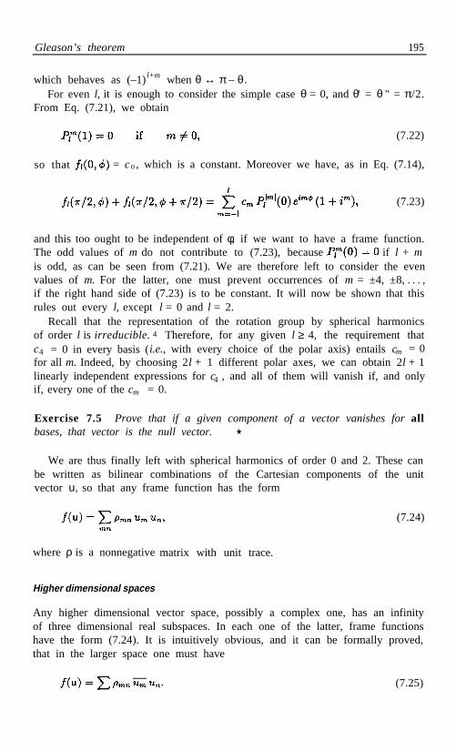
Gleason’s theorem 195
which behaves as (–1)l+m when θ ↔ π – θ.For even l, it is enough to consider the simple case θ = 0, and θ' = θ " = π/2.
From Eq. (7.21), we obtain
(7.22)
so that = co, which is a constant. Moreover we have, as in Eq. (7.14),
(7.23)
and this too ought to be independent of φ, if we want to have a frame function.The odd values of m do not contribute to (7.23), because if l + mis odd, as can be seen from (7.21). We are therefore left to consider the evenvalues of m. For the latter, one must prevent occurrences of m = ±4, ±8,. . . ,if the right hand side of (7.23) is to be constant. It will now be shown that thisrules out every l, except l = 0 and l = 2.
Recall that the representation of the rotation group by spherical harmonicsof order l is irreducible. 4 Therefore, for any given l ≥ 4, the requirement thatc4 = 0 in every basis (i.e., with every choice of the polar axis) entails cm = 0for all m. Indeed, by choosing 2l + 1 different polar axes, we can obtain 2l + 1linearly independent expressions for c4 , and all of them will vanish if, and onlyif, every one of the cm = 0.
Exercise 7.5 Prove that if a given component of a vector vanishes for allbases, that vector is the null vector.
We are thus finally left with spherical harmonics of order 0 and 2. These canbe written as bilinear combinations of the Cartesian components of the unitvector u, so that any frame function has the form
(7.24)
where ρ is a nonnegativematrix with unit trace.
Higher dimensional spaces
Any higher dimensional vector space, possibly a complex one, has an infinityof three dimensional real subspaces. In each one of the latter, frame functionshave the form (7.24). It is intuitively obvious, and it can be formally proved,that in the larger space one must have
(7.25)

196 Contextuality
A rigorous proof of this assertion involves intricate geometrical arguments, forwhich the interested reader is referred to Gleason’s original article.²
Cryptodeterminism
Gleason’s theorem is a powerful argument against the hypothesis that thestochastic behavior of quantum tests can be explained by the existence of asubquantum world, endowed with “hidden variables” whose values unambigu-ously determine the outcome of each test. If it were indeed so, then, for anyspecific value of the hidden variables, every elementary test (yes-no question)would have a unique, definite answer; and therefore every projector Pu wouldcorrespond to a definite value, 0 or 1. And therefore the functiontoo would everywhere be either 0 or 1 (its precise value depending on those ofthe hidden variables). Such a discontinuous function ƒ(u) is radically differentfrom the smooth distribution (7.25) required by Gleason’s theorem. This meansthat Eq. (7.5) cannot be valid, in general, for an arbitrary distribution of hiddenvariables; and therefore, a hidden variable theory must violate Postulate γ, aslong as the hidden variables have not been averaged over.
This conclusion was first reached by Bell.5 Soon afterwards, Kochen andSpecker6 gave a purely algebraic proof, which used only a finite number ofoperators (117 operators, to be precise). Gleason’s continuity argument, whichhad motivated the work of Bell and of Kochen and Specker, was no longer neededfor discussing the cryptodeterminism problem. More recent (and simpler) proofsof the Kochen-Specker theorem are given in the next section.
7-3. The Kochen-Specker theorem
The Kochen-Specker theorem asserts that, in a Hilbert space of dimensiond ≥ 3, it is impossible to associate definite numerical values, 1 or 0, with everyprojection operator Pm , in such a way that, if a set of commuting Pm satis-f ies , the corresponding values, namely v(Pm ) = 0 or 1, also satisfy
. The thrust of this theorem is that any cryptodeterministic theorythat would attribute a definite result to each quantum measurement, and stillreproduce the statistical properties of quantum theory, is inevitably contextual.In the present case, if three operators, Pm , P r , and P s , have commutators
and , the result of a measurement of Pm
cannot be independent of whether Pm is measured alone, or together with Pr ,or together with Ps .
Exercise 7.6 Write three projectors P m , P r , and Ps with the above algebraicproperties. Explain why this requires a vector space of dimension d ≥ 3.
5 J. S. Bell, Rev. Mod. Phys. 38 (1966) 447.6S. Kochen and E. Specker, J. Math. Mech. 17 (1967) 59.

The Kochen-Specker theorem 197
The proof of the theorem runs as follows. Let u1 , . . . , uN be a complete setof orthonormal vectors. The N matrices Pm = um u†
m are projection operatorson the vectors um . These matrices commute and satisfy There areN different ways of associating the value 1 with one of these matrices (that is,with one of the vectors u m ), and the value 0 with the N – 1 others. Considernow several distinct orthogonal bases, which may share some of their unit vec-tors. Assume that if a vector is a member of more than one basis, the value(1 or 0) associated with that vector is the same, irrespective of the choice of theother basis vectors. This assumption leads to a contradiction, as first shownby Kochen and Specker6 for a particular set of 117 vectors in 3 (the real3-dimensional vector space). The earlier proof by Bell5 involved a continuumof vector directions, but it can easily be rewritten in a way using only a finitenumber of vectors.
As this result has a fundamental importance, many attempts were made tosimplify the Kochen-Specker proof, and in particular to use fewer than 117vectors. The most economical proof known at present is due to Conway andKochen, who found a set of 31 vectors having the required property. Thedirection cosines of these vectors have ratios involving only small integers, 0,±1, and ±2 (see Plate II, page 114). Here however, we shall consider anotherset, with 33 vectors belonging to 16 distinct bases in3. That set enjoys manysymmetries which greatly simplify the proof of the theorem.7 We shall then seean even simpler proof in4, using only 20 vectors.
In these proofs, I shall use the word ray, rather than vector, because onlydirections are relevant. The length of the vectors never plays any role, and itis in fact convenient to let that length exceed 1. This does not affect orthogo-nality, and the algebra becomes easier. To further simplify the discourse, raysassociated with the values 1 and 0 will be called green and red, respectively (asin traffic lights, green = yes, red = no).
Thirty three rays in 3
The 33 rays used in the proof are shown in Fig. 7.2. They will be labelled xyz,where x, y, and z can be: 0, 1, (this symbol stands for –1), 2 (means ),and (means – ). For example the ray 02 connects the origin to the point
(–1, 0, ). Opposite rays, such as02 and 10 , are counted only once, becausethey correspond to the same projector.
Exercise 7.7 Show that the squares of the direction cosines of each ray areone of the combinations , and allpermutations thereof.
Exercise 7.8 Show that the 33 rays form 16 orthogonal triads (with each raybelonging to several triads).
7 A. Peres, J. Phys. A 24 (1991) L175.
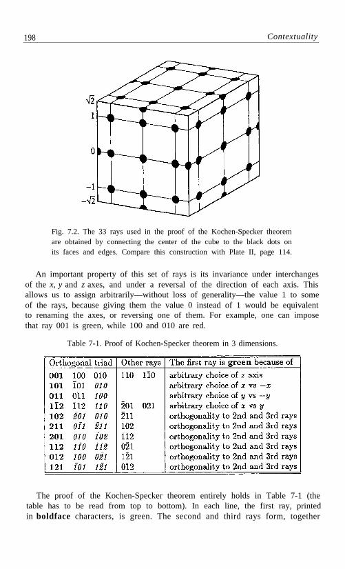
198 Contextuality
Fig. 7.2. The 33 rays used in the proof of the Kochen-Specker theoremare obtained by connecting the center of the cube to the black dots onits faces and edges. Compare this construction with Plate II, page 114.
An important property of this set of rays is its invariance under interchangesof the x, y and z axes, and under a reversal of the direction of each axis. Thisallows us to assign arbitrarily—without loss of generality—the value 1 to someof the rays, because giving them the value 0 instead of 1 would be equivalentto renaming the axes, or reversing one of them. For example, one can imposethat ray 001 is green, while 100 and 010 are red.
Table 7-1. Proof of Kochen-Specker theorem in 3 dimensions.
The proof of the Kochen-Specker theorem entirely holds in Table 7-1 (thetable has to be read from top to bottom). In each line, the first ray, printedin boldface characters, is green. The second and third rays form, together

The Kochen-Specker theorem 199
with the first one, an orthogonal triad. Therefore they are red. Additional rayslisted in the same line are also orthogonal to its first ray, therefore they too arered (only the rays that will be needed for further work are listed). When a redray is printed in italic characters, this means that it is an “old” ray, that wasalready found red in a preceding line. The choice of colors for the new raysappearing in each line is explained in the table itself.
The first, fourth and last lines contain rays 100, 021, and 0 2, respectively.These three rays are red and mutually orthogonal: this is the Kochen-Speckercontradiction. It can be shown that if a single ray is deleted from that set of33, the contradiction disappears. It is so even if the deleted ray is not explicitlylisted in Table 7-1. This is because the removal of one ray breaks the symmetryof the set and therefore necessitates the examination of alternative choices. Theproof that a contradiction can then be avoided is not as simple as in Table 7-1(the computer program in the Appendix may help).8
Physical interpretation
Since our present Hilbert space is isomorphic to ³, the abstract vectors u m be-have as ordinary Euclidean vectors. We shall therefore denote them by boldfaceletters, m, n, etc. A simple physical interpretation of the projection operatorP m can be given in terms of the angular momentum components of a spin 1particle. It is convenient to use a representation where
(7.26)
in natural units ( = 1). These matrices satisfy[J x , Jy] = i J z , and cyclicpermutations thereof. With this representation, we have
(7.27)
These three matrices commute, so that the corresponding observables can bemeasured simultaneously. One may actually consider all the J m
2 as functionsof a single nondegenerate operator,
8 The proof originally given by Kochen and Specker proceeds in two steps. The first step(which is the difficult one) is a lemma saying that two particular vectors out of a given set of8 vectors cannot both have the value 1. The second, much easier step is to replicate 15 timesthat 8-vector set, in a way leading to a contradiction. Three of the vectors appear twice in thisconstruction, making a total of 15 × 8 – 3 = 117 distinct vectors. Some authors consider thesecond step so trivial that they say that the Kochen-Specker proof necessitates only 8 vectors(and then Bell’s earlier proof would have used 10 vectors). However, the purists, includingKochen and Specker themselves, want a complete proof, not only a lemma, and their count is117 vectors.

200 Contextuality
(7.28)
Exercise 7.9 Show that , and write likewise Jy ² and J z²
as functions of K.
Exercise 7.10 Write explicitly the three matrices Jk J l + J l J k (for k ≠ l) andshow that, for any real unit vector m, the matrix
has components (P m ) rs = m r m , and therefore is a projection operator.s
A measurement of the projector P is a test of whether the spin componentm
along the unit vector m is equal to zero. The eigenvalue 1 corresponds tothe answer “yes,” and the degenerate eigenvalues 0 to the answer “no.” Notethat this test is essentially different from an ordinary Stern-Gerlach experimentwhich would measure the spin component along m, because the degeneratematrix P m makes no distinction between the eigenvalues –1 and +1 of m ⋅ ⋅ J .
A generalization of (7.28), for two orthogonal unit vectors m and n, is
This operator has eigenvalues –1, 0, and 1. A direct measurement of K (m,n)is difficult, but it is technically possible,³ and a single operation can therebydetermine the “colors” of the triad m, n and m × n.
The 33 rays that were used in the proof of the Kochen-Specker theorem form16 orthogonal triads (see Exercise 7.8). These triads correspond to 16 differentand noncommuting operators of the same type as K (m, n). Any one of them,but only one, can actually be measured. The results of the other measurementsare counterfactual—and mutually contradictory.
4
(7.29)
(7.30)
Twenty rays in
Consider again our pair of spin12 particles. Recall that in array (7.1), each rowand each column is a complete set of commuting operators. The product ofthe three operators in each row or column is , except those of the thirdcolumn, whose product is It is obviously impossible to associate, witheach one of these nine operators, numerical values 1 or –1, that would obey thesame multiplication rule as the operators themselves.
This algebraic impossibility will now be rephrased in the geometric languageof the Kochen-Specker theorem. The common eigenvectors of the commutingoperators in each row and each column of (7.1) form a complete orthogonal basis.We thus have 6 orthogonal bases, with a total of 24 vectors. The impossibleassignment is to “paint” them in such a way that one vector of each basis is
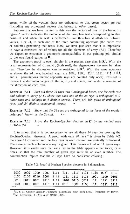
The Kochen-Specker theorem 201
green, while all the vectors thata are orthogonal to that green vector are red(including any orthogonal vectors that belong to other bases).
Suppose that we have painted in this way the vectors of one of the bases. Its“green” vector indicates the outcome of the complete test corresponding to thatbasis—if and when the test is performed—and therefore it attributes definitevalues, 1 or –1, to each one of the three commuting operators (the entire rowor column) generating that basis. Now, we have just seen that it is impossibleto have a consistent set of values for all the elements of array (7.1). Thereforewe expect to encounter a geometric incompatibility in our painting job, similarto the one found earlier in3.
The geometric proof is even simpler in the present case than in3. With theusual representation of σz and σ x (both real), the eigenvectors too may be takenreal. Therefore the discussion can be restricted to4. With the same notationsas above, the 24 rays, labelled wxyz, are 1000, 1100, 1 00, 1111, 111 11, ,and all permutations thereof (opposite rays are counted only once). This set isinvariant under interchanges of the w, x, y and z axes, and under a reversal ofthe direction of each axis.
Exercise 7.11 Sort out these 24 rays into 6 orthogonal bases, one for each rowand column in array (7.1). Show that each one of the 24 rays is orthogonal to 9other rays and belongs to 4 distinct tetrads. There are 108 pairs of orthogonalrays, and 24 distinct orthogonal tetrads.
Exercise 7.12 Show that the 24 rays are orthogonal to the faces of the regularpolytope 9 known as the 24-cell.
Exercise 7.13 Prove the Kochen-Specker theorem in 4 by the method usedin Table 7-1.
It turns out that it is not necessary to use all these 24 rays for proving theKochen-Specker theorem. A proof with only 20 rays10 is given by Table 7-2:there are 11 columns, and the four rays in each column are mutually orthogonal.Therefore in each column one ray is green. This makes a total of 11 green rays.However, it is easily seen that each ray in the table appears either twice, or 4times, so that the total number of green rays must be an even number. Thecontradiction implies that the 20 rays have no consistent coloring.
Table 7-2. Proof of Kochen-Specker theorem in 4 dimensions.
9 H. S. M. Coxeter, Regular Polytopes, Macmillan, New York (1963) [reprinted by Dover].10M. Kernaghan, J. Phys. A 27 (1994) L829.

202 Contextuality
7-4. Experimental and logical aspects of contextuality
The Kochen-Specker theorem is a geometrical statement. Like Bell’s theorem,it is independent of quantum theory, but it profoundly affects the interpretationof the latter. However, the Kochen-Specker theorem, contrary to Bell’s, doesnot involve statistical correlations in an ensemble of systems. It compares theresults of various measurements that can be performed on a single system. Thisis a radical simplification. There is no need of taking averages over unspecifiedhidden variables, or over fictitious experimental runs, as in the derivation ofthe CHSH inequality from Eq. (6.29). Moreover, the absence of statisticalconsiderations relieves us of any worries about detector efficiencies.
Yet, the problem cannot be one of pure logic. Any discussion about physicsmust ultimately make connection with experimental facts. The purpose of thissection is to analyze the empirical premises underlying the theorems of Belland of Kochen and Specker. These premises are formulated as nine distinctpropositions. Seven of them are strictly phenomenological. They can be testedexperimentally (in addition to tests for internal consistency). They can also bederived from quantum theory.
The last two propositions are of counterfactual nature: They state that it ispossible to imagine the results of unperformed experiments, and moreover, todo that in such a way that these hypothetical results have correlations whichmimic those of actual experimental results. Although this counterfactual rea-soning appears reasonable, it produces inadmissible consequences such as Bell’sinequality, which is experimentally violated, or the Kochen-Specker coloringrule for vectors, which is contradictory.
A. Elementary tests
We start with some definitions and propositions which are not controversial.
There are “elementary tests” (yes-no experiments) labelled A, B, C, . . . Theiroutcomes are labelled a, b, c, ⋅ ⋅ ⋅ = 1 (yes) or 0 (no).
In quantum theory, these elementary tests are represented by projection oper-ators. It is sufficient here to consider only a subset of quantum theory, whereprojectors are represented by real matrices of order 2 or 3.
Exercise 7.14 Show that any 3 × 3 real projector with unit trace can bewritten as in Eq. (7.29).
Exercise 7.15 Show that any 2 × 2 real projector with unit trace can bewritten as
(7.31)
A physical realization of Pθ may be a Stern-Gerlach test of spin– particles, forwhich Pθ represents the question “Is the component of spin along the θ direction
12

Experimental and logical aspects of contextuality 203
positive?” Another possible implementation may involve the linear polarizationof photons.
B. State preparation
In general the outcome of a given test cannot be predicted with certainty. Yet,the following exception holds:
For each elementary test, there are ways of preparing physical systems so thatthe outcome of that test is predictable with certainty.
In quantum theory, a preparation is represented by a density matrix ρ. Theresult of an elementary test represented by a projector P is predictable if andonly if Tr (ρP) = 0 or 1. In general, the preparation satisfying this equation isnot unique, because P may be degenerate.
C. Compatibility of elementary tests
Some tests are compatible. Compatibility is defined as follows:
If a physical system is prepared in such a way that the result of test A i spredictable and repeatable, and if a compatible test B is then performed(instead of test A) a subsequent execution of test A shall yield the same resultas if test B had not been performed.
In quantum theory, compatibility occurs when operators A and B commute.We have seen in Sect. 2-2 that not every test is repeatable but, for our presentpurpose, it is enough to consider repeatable tests, which certainly exist.
A familiar pair of commuting projectors which represent compatible tests is:
(7.32)
where m and n are arbitrary unit vectors, and σ1 and σ2 refer to two distinctspin - particles. Another example of commuting projectors is1
2
(7.33)
where J refers to a single particle of spin 1, and m · n = 0.
Remark: If we wished to extend these notions to classical physics, we wouldfind that all tests are compatible.
D. Symmetry and transitivity
Compatibility is a symmetric property, but it is not transitive.
This statement means that if A is compatible with B, then B is compatible withA (this is not obvious, but this follows from quantum theory and this can alsobe tested experimentally). However, if A is compatible with B and with C, itdoes not follow that B is compatible with C.

204 Contextuality
Exercise 7.16 For a spin 1 particle, define
(7.34)
with m · n = m · r = 0 ≠ n · r. Show that [A, B] = [A, C] = 0 ≠ [B, C].
Exercise 7.17 Show the same for two spin –1 particles, with the definitions2
(7.35)
Remark: It is implicit that compatibility is a reflexive property (this followsfrom [A, A] ≡ 0). If any test is repeated, it will give the same result. As alreadystated, the present discussion is restricted to repeatable tests.
E. Constraints
When a state preparation is such that compatible tests have predictable results,these results may be constrained.
+ p
Example (spin 1): Let m, n, r be three orthogonal unit vectors and let us define, corresponding to the question “Is m · J = 0?”. Likewise
define projectors Pn and Pr . The three corresponding tests are compatible, aswe have seen. Moreover, we have
(7.36)
Quantum theory predicts, and it can in principle be tested experimentally, thatfor state preparations such that the outcomes of these three tests are predictable,their outcomes satisfy
(7.37)
One test is positive and two are negative.
Warning: At this point, we may imagine hypothetical systems subject to con-straints that lead to logical contradictions. For example, if we have four distincttests such that any three are subject to a constraint like (7.37), we obtain
a + b + c = 1, a + b + d = 1, a + c + d = 1, b + c + d = l, (?)
whence 3(a + b + c + d ) = 4, which is obviously impossible. Of course, thereis no physical system obeying these rules! The important point to notice hereis that innocent looking postulates, such as those that we are proposing here,may lead to contradictions. We are always free to propose postulates, but wemust carefully check them for internal consistency.
Example (spin 12 ) : If the test for has a predictable outcome
p m , then pm – m = 1.

Experimental and logical aspects of contextuality 205
F. Further constraints
The preceding postulate referred to state preparations leading to predictableresults. It has the following generalization:
Even if a system is prepared in such a way that the outcomes of constrainedtests are not predictable, these outcomes will be found to satisfy the properconstraints, if the tests are actually performed.
In other words, even if the outcomes of individual tests are not predictable, theyare not completely random. There appears to be some law and order in nature.This may encourage us to think in terms of a microphysical determinism, andperhaps to attempt to introduce hidden variables. This is not, however, thepath followed here.The present discussion is strictly phenomenological (anyreference to quantum theory is merely illustrative).
This last proposition can be tested experimentally. It can also be derivedfrom quantum theory, if we wish to use the latter. A complete set of orthogonalprojectors satisfies and We then have, for thecorresponding outcomes (p i = ±1):
(7.38)
s o that ∑ pi = 1 always (this result is dispersion free).
Remark: The derivation of (7.38)assumes that, for orthogonal projectors, theaverage of a sum is the sum of averages. This rule is amenable to experimentalverification. See the discussion that follows Eq. (7.5).
Remark: Postulate F has no classical analog (if it had one, there would bean inconsistency of the Kochen-Specker type in classical physics, because allclassical tests are compatible).
G. Correlations
As an example, consider a pair of spin12
particles, prepared in a singlet state.Define projectors where α and βare unit vectors. Let p1α and p 2β be the outcomes (0 or 1) of the measurementsof P 1α and P 2β , respectively. We then have, on the average,
A weaker form of the preceding postulate is the following statement:
If an ensemble of systems is prepared in such a way that the outcomes of severalcompatible tests are neither predictable nor constrained, there may still bestatistical correlations between these outcomes.
and
(7.39)
Exercise 7.18 Show that , and that (7.39) is just another way ofwriting the spin correlation in Eq. (6.23).

206 Contextuality
Again, this refers to a purely intellectual exercise. For example, if we have apair of spin -1 particles, and we measure P
2 1α on the first one, we can measureeither P 2β or P 2δ on the second particle. These are two different (and mutuallyincompatible) setups, for which can imagine 2³= 8 different sets of outcomes.We cannot know which one of these outcomes will turn out to be true, butwe certainly can consider all eight possibilities. We can imagine that theseexperiments are repeated many times, after preparing the particle pairs in asinglet state. The hypothetical results must then be chosen so as to satisfycorrelations such as Eq. (7.39) and also
Note that we want both (7.39) and (7.40) to be satisfied, although only one ofthe two experiments can actually be performed on any given pair of particles.
We already know that this correlation violates Bell’s inequality. However, inorder to derive that inequality, or to prove the Kochen-Specker theorem, weneed two additional postulates, of a radically different nature.
In the present discussion, hidden variables are not used explicitly, nor evenimplicitly by assuming some unspecified kind of determinism. We shall onlyconsider what could have possibly been the results of unperformed experiments,had these experiments been performed.
a) It is possible to imagine hypothetical results for any unperformed test, and todo calculations where these unknown results are treated as if they were definitenumbers.
H. Counterfactual realism
This statement refers to a purely intellectual activity and there can be no doubtthat it is experimentally correct. For example, we can very well imagine thepossible results of a test Pm . The latter can only be 1 (yes) or 0 (no). We canthen perform a set of calculations assuming that the result was 1, and another,different set of calculations, assuming that the result was 0. There is nothingto prevent us from doing the same intellectual exercise for other possible tests,P n , P r , etc., even if the latter are mutually incompatible.
b) It is furthermore possible to imagine the results of any set of compatibletests, and to treat them in calculations as if these sets of results had definitevalues, satisfying the same constraints or correlations that are imposed on theresults of real tests.
Likewise, for a spin 1 particle, we can consider two orthonormal triads sharingone unit vector: m · n = m · r = n · r = 0 and m · s = m · t = s · t = 0. However,n ⋅ s ≠ 0. For example, . We can now imagine that we measure,together with , either P n and Pr , or P s and P t (theseprojectors are defined in the same way as Pm ). The results of these hypotheticalmeasurements must then obey both
(7.40)

Experimental and logical aspects of contextuality 207
(7.41)
and
(7.42)
We can for sure write these two equations, although at most one of them canmaterialize experimentally in a test performed on a given spin 1 particle.
Here however, there is a rather subtle difficulty: Is pm in (7.41) the same asp m in (7.42)? This cannot be tested experimentally, because these two setupsare mutually incompatible. We therefore propose one more postulate:
I . Counterfactual compatibility
The hypothetical result of an unperformed elementary test does not depend onthe choice of compatible tests that may be performed together with it.
This is the crucial “no-contextuality” hypothesis. For example, the result of ameasurement of P 1α on a spin 1 particle does not depend on whether one elects2to measure P
–
2β or P 2δ on a second, distant particle. Likewise, the outcome p m
is the same whether one elects to measure P n and P r , as in Eq. (7.41)‚ or P s
and P t , as in Eq. (7.42).The “psychological reason” suggesting the validity of this last postulate is
that, whenever a state preparation guarantees a predictable result for sometest, this result is not affected by performing other, compatible tests. One isnaturally tempted to generalize this property (just as Postulate F generalizedPostulate ε) to counterfactual tests whose outcome is not predictable.
Summary
Although counterfactual compatiblity cannot be tested directly, some of itslogical consequences can be shown to conflict with quantum theory—and withexperimental results. For example, it can be seen, by direct inspection, that
(7.43)
Exercise 7.19 Show that no other value is possible.
Therefore, the average value of the left hand side of (7.43) ought to be in therange [0,1]. This is just another form of Bell’s inequality.11 Nevertheless, bychoosing the directions α, β, γ and δ as in Fig. 7.3, the left hand side of (7.43)becomes, on the average, for a pair of spin1–2 particles in the singlet state,
(7.44)
11J. F. Clauser and M. A. Horne, Phys. Rev. D 10 (1974) 526.

208 Contextuality
contrary to the counterfactual prediction in (7.43).Likewise, Table 7-1 shows that it is possible to choose 33 rays in such a way
that Eqs. (7.41) and (7.42) lead to a contradiction, if it is assumed that each oneof the outcomes p m‚ p n‚ etc., has the same numerical value in all the equationswhere it appears.
Fig. 7.3. The four directionsused in Eqs. (7.43) and (7.44)make angles of 45°.
The rationale behind quantum contextuality is the following: An elementarytest such as “Is α · σ 1 = l?” or “Is m · J = 0?” has a well defined answeronly if the state preparation satisfies Tr (ρP) = 0 or 1, so that the requiredanswer is predictable. For any other state preparation, these questions, whichare represented by degenerate operators, are ambiguous. The answer dependson which other (compatible) tests are performed, for example, on whether weshall also measure n · σ2 , or r · σ2, together with m · σσ 1.
This state of affairs can be succintly summarized: The same operator maycorrespond to different observables. That is, a given Hermitian matrix Pm doesnot represent a unique “observable.”The symbol Pm has a different meaning ifPm is measured alone, or measured with Pn , or with Pr . The only exceptionis a nondegenerate variable, such as K (m, n) in Eq. (7.30), which is equivalentto a complete set of commuting observables, corresponding to compatible tests.One then effectively has a complete test, rather than an elementary one, andcontextuality effects do not appear.
This mismatch of operators and observables was first mentioned by Bell5 inhis analysis of the implications of Gleason’s theorem:
It was tacitly assumed that measurement of an observable must yield thesame value independently of what other [compatible] measurements maybe made simultaneously . . . There is no a priori reason to believe that theresults should be the same. The result of an observation may reasonablydepend not only on the state of the system (including hidden variables)but also on the complete disposition of the apparatus . . .”
The notion of contextuality appears even earlier, in the writings of Bohr12 whoemphasized “the impossibility of any sharp distinction between the behavior ofatomic objects and the interaction with the measuring instruments which serveto define the conditions under which the phenomena appear.”
1 2 N. Bohr, in Albert Einstein, Philosopher-Scientist, ed. by P. A. Schilpp, Library of LivingPhilosophers, Evanston (1949), p. 210.

Appendix: Computer test for Kochen-Specker contradiction 209
7-5. Appendix: Computer test for Kochen-Specker contradiction
The proof of the Kochen-Specker theorem given in Table 7-1 was very simple,because the rays formed a highly symmetrical pattern. It was possible to choosearbitrarily, in some of the triads, the “green” rays to which the value 1 wasassigned, because any other choice would have been equivalent to a relabellingof the coordinates.
When there is less symmetry, as in the case of the 31 rays of Plate II (p. 114),different assignments of the value 1 are not equivalent to renaming the axes.Therefore both values, 0 and 1, must be tried. If one of them leads to aninconsistency, one still has the other choice to try. The search for a consistentcoloring is similar to the search for a passage through a maze. Whenever theexplorer reaches a dead end, he has to retrace his footsteps to the last pointwhere he made an arbitrary choice, and try another choice.
The following FORTRAN code performs this search for any pattern of N rays.The input file is a list of all orthogonal pairs of rays. This list, which describesthe geometric structure of the set of rays, must be supplied by the user. Theoutput file returns a string of 0 and 1, if the N rays can be consistently colored,or a message stating that no coloring is possible.
C
CCCCCCC
C
10
C
1112
C
Kochen-Specker coloring problem for N raysPARAMETER (N= )INTEGER P(N,N), X(N), Y(N), Z(N), C(N), L(N), OC(N,N)P(I,J)=1 if rays I and J are orthogonal, else P(I,J)=0NTRIAD is number of orthogonal triadsX(NT), Y(NT), Z(NT) are the three rays in triad NTC(J) is color of ray J: 0 = red, 1 = green, 4 = unknownLVL = number of rays whose color was arbitrarily chosenL(K) is the ray whose color was assigned in Kth choiceOC(LVL,J) was color of ray J after LVL arbitrary choicesOPEN (8,FILE='INPUT.KS')OPEN (9,FILE='OUTPUT.KS')DO 10 I=1,NC(I)=4Colors are unknown as yetDO 10 J=1,NP(I,J)=0DO 11 M=1,N*NRead list of pairs of orthogonal raysREAD (8,'(2I3)',END=12) I, JP(I,J)=1P(J,I)=1NTRIAD=0Find triads of orthogonal raysDO 13 I=1, N

210 Contextul i ty
DO 13 J=I+1,NDO 13 K=J+1,NIF (P(I,J)+P(I,K)+P(J,K).NE.3) GOTO 13NTRIAD=NTRIAD+1X(NTRIAD)=IY(NTRIAD)=JZ(NTRIAD)=K
13 CONTINUELVL=0
C Choose arbitrarily next green ray, whose number is NGC All other rays that are already colored are consistent14 DO 15 NG=1,N
IF (C(NG).EQ.4) THENC(NG)=1GOTO 16
ENDIF15 CONTINUE
WRITE (9,'(40I2)') CC A consistent coloring has been found
STOP16 LVL=LVL+1
LAST=1C Last arbitrary assignment was to make a ray green
L(LVL)=NGC This arbitrary assignment was made for ray NG
DO 17 J=1,NC Record the situation after LVL arbitrary choices17 OC(LVL,J)=C(J)18 DO 19 J=1,N
C All the rays orthogonal to a green one must be red19 IF (P(NG,J).EQ.1) C(J)=020 DO 21 NT=1,NTRIADC Now check whether there are three orthogonal red rays
IF (C(X(NT))+C(Y(NT))+C(Z(NT)).EQ.0) GOTO 2221 CONTINUE
GOTO 2522 IF (LVL+LAST.GT.0) GOTO 23
WRITE (9,'(" No consistent coloring")')C All options have been exhausted
STOP23 DO 24 J=1,NC Restore status quo at preceding branching24 C(J)=OC(LVL,J)
C(L(LVL))=0LAST=0

Bibliography 211
C
C
25CC
26
27
Last arbitrary assignment was to make a ray redLVL=LVL-1Return to preceding branchingGOTO 20DO 26 NT=1,NTRIADIs there a triad with two red rays and a colorless ray?If so, the colorless ray must be painted greenIF (C(X(NT))+C(Y(NT))+C(Z(NT)).EQ.4) GOTO 27CONTINUEGOTO 14IF (C(X(NT)).EQ.4) THEN
C(X(NT))=1NG=X(NT)GOTO 18
ENDIFIF (C(Y(NT)).EQ.4) THEN
C(Y(NT))=1NG=Y(NT)GOTO 18
ENDIFIF (C(Z(NT)).EQ.4) THEN
C(Z(NT))=1NG=Z (NT)GOTO 18
ENDIFEND
Exercise 7.20 Show that the 31 rays in Plate II (p. 114) form 71 orthogonalpairs, which belong to 17 orthogonal triads.
Exercise 7.21 Show that removing any one of these 31 rays leaves a set thatcan be consistently colored.
Exercise 7.22 Write a similar program for the Kochen-Specker problem infour dimensions.
7-6. Bibliography
F. J. Belinfante, A Survey of Hidden-Variable Theories, Pergamon, Oxford(1973).
M. Redhead, Incompleteness, Nonlocality, and Realism, Clarendon Press,Oxford (1987).
These excellent books are unfortunately obsolete, because of the recent developmentsdiscussed in this chapter and the preceding one.

212 Contextuality
and (7.45)
N. D. Mermin, “Simple unified form for the major no-hidden-variablestheorems,” Phys. Rev. Lett. 65 (1990) 3373; “Hidden variables and the twotheorems of John Bell,” Rev. Mod. Phys. 65 (1993) 803.
J. Zimba and R. Penrose, “On Bell non-locality without probabilities: morecurious geometry,” Studies in History and Philosophy of Science, 24 (1993) 697.
This paper contains an elegant proof of the Kochen-Specker theorem, involving thegeometric properties of the dodecahedron. The proof is based on the following propertyof spin –3
2particles: the eigenvectors ψ and φ, satisfying
are orthogonal if m · n = 1/3. Recall that cos–1(1/3) is the angle subtended at thecenter of a dodecahedron by a pair of next-to-adjacent vertices. Thus, if we considerthe results of (mutually incompatible) spin measurements which test whether the spincomponents along the 20 directions pointing toward the vertices of a dodecahedron areequal to 1 , we obtain the following Kochen-Specker coloring rules:–
2
(a) no two next-to-adjacent vertices can be green,
(b) the six vertices adjacent to any pair of antipodal vertices cannot all be red.
Rule (a) follows from the orthogonality property mentioned above, and rule (b) can beproved by introducing 20 additional, “implicit” state vectors,8 one for each vertex of thedodecahedron, in the following way: Each vertex Vk has three adjacent vertices, whichare next-to-adjacent to each other. Therefore the three eigenvectors of type (7.45),
corresponding to these three vertices, are mutually orthogonal (in Hilbert space). Thefourth orthogonal vector (in Hilbert space) is the “implicit vector” belonging to vertexV k . It is easily shown that coloring rules (a) and (b) lead to a contradiction.13
Higher dimensions
A set of Kochen-Specker vectors for any dimension n > 3 is always obtainable froma set of dimension n–1 as follows: add to all these vectors a null n -th component, andintroduce a new vector 0. . . 01. The only consistent coloring is to make the new vectorgreen and all the others red. The latter include 10. . . 0. Now introduce more vectors byexchanging the first and n -th components of all the preceding ones. The complete sethas no consistent coloring. However, much smaller sets can be obtained in some cases:
M. Kernaghan and A. Peres, “Kochen-Specker theorem for eight-dimensionalspace,” Phys. Letters A 198 (1995) 1.
A contradiction is derived for a system of three entangled spin-1– particles (see2
page 152). The proof requires 36 vectors. This article also introduces a “state-specific”version of the Kochen-Specker theorem, valid for systems that have been prepared ina known pure state. The projection operators can then be chosen in a way adapted tothe known state, and fewer operators are needed (only 13 in the present case).
13 Penrose, who first stated that proof in an unpublished article, also showed that the 33 raysof Table 7-1 can be generated by three interpenetrating cubes, as those in Escher’s celebratedlithograph Waterfall. For further details, see Scientific American 268 (Feb. 1993) 12.

Part III
QUANTUM DYNAMICS
AND INFORMATION

Plate III. Musical notation as shown above contains information on time and onfrequency. These are complementary parameters, which satisfy the “uncertaintyrelation” ∆ t ∆ ω ≥ 1
2– (this inequality is a general property of Fourier transforms).Show that this limitation does not cause any serious difficulty in playing music,because the uncertainty area is quite small on the scale of the above figure. Yet,if you try to play very low notes, for example with a double bass, it is difficult tomake these notes very brief. Because of the way music is written, the time scale inthis figure is not linear, and the frequency scale is only approximately logarithmic.One quaver (eighth note) is about 0.22s. The figure is from a work of Mozart.*
*W. A. Mozart, Duet for violin and viola in B flat major (K. 424).
214
Chapter 8
(8.1)
Spacetime Symmetries
8-1 . What is a symmetry?
A symmetry is an equivalence of different physical situations. The hallmarkof a symmetry is the impossibility of acquiring some physical knowledge.¹ Forexample, it is impossible to distinguish a photograph depicting a right handglove from one of a left hand glove, viewed in a mirror.
The laws of nature that you observe in your laboratory are also valid inother laboratories: these laws are invariant under translations and rotationsof the scientific instruments that are used to verify them. Moreover, they areinvariant under a uniform motion of these instruments. This is a kinematicsymmetry, first postulated by Galilei for mechanical laws, and later found validby Michelson and Morley for optical phenomena in vacuum. Einstein proposedthat this symmetry applies to electromagnetism in general. This is the principleof relativity, which is today firmly established for all physical phenomena, withthe possible exception of gravitation.²
Active and passive transformations
The existence of a symmetry entails the equivalence of two types of transforma-tions, called active and passive. For example, the hand sketched in Fig. 8.1(a)is actively rotated, with no change of shape, into a new position. The newcoordinates (of the fingertip, say) are related to the old ones by
¹F. E. Low, Comm. Nucl. Particle Phys. 1 (1967) 1.²According to the general theory of relativity, the description of gravitational phenomena
necessitates the use of a non-Euclidean geometry which does not allow rigid motions of ex-tended bodies, such as laboratory instruments. Therefore general relativity, contrary to specialrelativity, is not the theory of a spacetime symmetry. (There are nevertheless exact solutionsof the Einstein gravitational field equations with restricted symmetry properties, for examplea spherically symmetric black hole.)
215

216 Spacetime Symmetries
In Fig. 8.1(b), the hand is not rotated, but the coordinates are, by the sameangle. This is a passive transformation, and the components of the fingertipalong the new axes are:
Obviously, the transformation matrix in (8.2) is the inverse of the one in (8.1).Therefore, if both transformations (active and passive) are simultaneously per-formed, as in Fig. 8.1(c), we obtain:
and (8.3)
The numerical values of the new components are the same as those of the oldcomponents. The mere knowledge of these values does not indicate whether atransformation was performed.
(8.2)
Fig. 8.1. Active and passive transformations.
This indistinguishability is due to a physical property of plane surfaces: itis possible to rigidly rotate any plane figure. On the other hand, an irregularsurface does not allow rigid motions. It still allows, of course, passive coordi-nate transformations, which are nothing more than a relabelling of its points,but there are no corresponding active transformations, which would leave thedisplaced body unaltered.2
Exercise 8.1 If we turn a right hand glove inside out, it becomes a left handglove (assume that the inside and outside textures are indistinguishable—agood approximation for some knitted gloves). This is an example of activetransformation. What is the corresponding passive transformation?
We now turn our attention to quantum symmetries. Quantum states arerepresented by vectors in a Hilbert space and can again be specified by a setof components. The indices which label these components refer to the possibleoutcomes of a maximal quantum test (see Sect. 3-l). A passive transformation

Wigner’s theorem 217
corresponds to the choice of a different basis—that is, a different maximal test—and it is represented by a unitary operator. On the other hand, an activetransformation is an actual change of the state of the quantum system.
As usual, the existence of a symmetry implies a correspondence betweenactive and passive transformations. Thus, if we choose another maximal testto define a new basis for the Hilbert space of states, we may expect that thereis an active transformation such that the new physical state, obtained afterthat transformation, has components with respect to the new basis, which areequal to the components of the original state with respect to the old basis—just as in Eq. (8.3). Actually, the situation is more complicated, because thevector space used in quantum theory is complex, and there is no one-to-onecorrespondence between physical states and sets of vector components. Thebasis vectors defined by maximal tests may be multiplied by arbitrary phases,inducing a phase arbitrariness in the components of the vector that representsa given physical state.
However, the transition probabilities Puv = ⟨ u, v ⟩ ², which are experimentallyobservable, are not affected by this phase arbitrariness. For example, vector umay represent photons in a horizontal beam, with a vertical polarization; andvector v, photons in the same beam, but with a linear polarization at an angle θfrom the vertical. Suppose that the apparatus which prepares u photons, andthen tests whether they are v photons, is rigidly moved to another location andgiven a different orientation. With respect to the original basis chosen in Hilbertspace, the photons are now prepared with a different polarization u', and testedfor a different polarization v'. Yet, the laws of optics are not affected by rigiddisplacements of optical instruments. Therefore the probability of passing thetest is invariant:
8-2. Wigner’s theorem
This invariance has far-reaching implications, because of an important theorem,due to Wigner.³ Consider a mapping of Hilbert space: , and soon. The only thing we assume about this mapping is that
(8.4)
In particular, we do not assume linearity, let alone unitarity. Wigner’s theoremstates that it is possible to redefine the phases of the new vectors (u ', v ', . . . )in such a way that, for any complex coefficients α and β , we have either
and (8.5)
or
and (8.6)
³E. P. Wigner, Group Theory, Academic Press, New York (1959) p. 233.

218 Spacetime Symmetries
In the first case, the mapping is linear and unitary, in the second case, it isantilinear and antiunitary. The proof of Wigner’s theorem follows.
Let e j be the vectors of an orthonormal basis, which are mapped into e'j .The new vectors e'j are also orthonormal, by virtue of Eq. (8.4). Consider nowthe set of vectors
(8.7)
which are mapped into f'j . We have, from (8.4),
(8.8)
and
(8.9)
Therefore, for any j > 1, we can write
(8.10)
where = 1. We then redefine the phases of the transformed vectors:
and (8.11)
(and e "1 = e'1 ) so as to obtain
(8.12)
as in (8.7). We shall henceforth work with the new phases, and write e'j insteadof e"
j. We thus have the mapping
Consider now the mapping of an arbitrary vector
(8.13)
(8.14)
We have
Moreover,
and
It then follows from Eqs. (8.4) and (8.13) that
(8.15)
(8.16)
(8.17)
Wigner’s theorem 219
(8.18)
Together with (8.15), this gives
Dividing this equation by
we obtain
which has the form
with two solutions, θ' = ± θ. Let us consider them one after another.
Unitary mapping: If θ ' = θ , we have
(8.19)
(8.20)
(8.21)
(8.22)
Redefine the phase of u' so that a'1 = a 1 . We then have and itfollows from (8.15) that a'j = a j . Therefore
(8.23)
Given another vector, , we can likewise choose the phase of v' so asto have , whence Eq. (8.5) readily follows.
Antiunitary mapping: If θ' = – θ, we have
(8.24)
Redefine the phase of u' so that . We then have and itfollows from (8.15) that . Therefore
(8.25)
Given another vector, , we can likewise choose the phase of v' so asto have v' = , which gives Eq. (8.6).
Whether a specific transformation is unitary or antiunitary depends on itsphysical nature. Transformations that belong to a continuous group, such astranslations and rotations, can only be unitary, because in that case any finitetransformation can be generated by a sequence of infinitesimal steps, where thetransformed vectors e'i are arbitrarily close to ei ; we must then choose
220 Spacetime Symmetries
(rather than ) if we want u' to be close to u. This rules out antiunitarytransformations.
On the other hand, this continuity argument is not applicable to discretetransformations, such as space reflection or time reversal. We shall later seethat a space reflection is represented by a unitary transformation, but a timereversal is antiunitary.
Finally, we note that the same results can be derived from premises weakerthan Eq. (8.4), by merely assuming that ⟨ u, v⟩ = 0 implies ⟨ u', v'⟩ = 0. In thatcase, however, the proof is much more difficult.4,5
8-3. Continuous transformations
Consider a set of unitary matrices , depending on continuous pa-rameters α j . These matrices are in one-to-one correspondence with the elementsof a continuous group of transformations, provided that the domain of definitionof the parameters α j is chosen in such a way that:
1) One, and only one, of these matrices is the unit matrixto define the parameters α j in such a way that
. It is customary
2) Every product of two matrices also is a member of that set of matrices.
3)choice of the parameters α j , there also are parameters β j , in the givendomain of definition, such that
Every matrix of the set has a unique inverse in that set, that is, for every
The fourth characteristic property of a group, which is the associative law,A(BC) = (AB)C, is automatically satisfied by matrices.
Exercise 8.2 Give examples of continuous transformations which do n o tsatisfy one or more of the above criteria, if the domain of definition of theparameters is not properly chosen.
A unitary matrix which is nearly equal to the unit matrix corresponds toan infinitesimal transformation (the unit matrix itself generates the identitytransformation). The importance of infinitesimal transformations stems fromthe fact that any finite unitary transformation can be obtained by exponentia-tion of an infinitesimal one. For example, a finite rotation in the complex planeis represented by a factor e iθ, which is the limit ofIn this case, is a trivial unitary matrix of order 1. More generally, forany Hermitian matrix H,
4 G. Emch and C. Piron, J. Math. Phys. 4 (1963) 469.5 N. Gisin, Am. J. Phys. 61 (1993) 86.

Continuous transformations 221
(8.26)
is a unitary matrix, as can easily be seen by writing this equation in the basiswhich diagonalizes H (and therefore also diagonalizes U ). Actually, it is oftenmore convenient to use the antihermitian matrix A = –i H, and to write
(8.27)
Transformations of operators
If we take a new basis for parametrizing the Hilbert space H , the componentsof the state vector ψ undergo a unitary mapping, , as we haveseen in Eq. (3.8). The corresponding transformation law of operators is
(passive transformation) (8.28)
so that the mean values remain invariant. Indeed, these average values,which are experimentally observable, cannot depend on the arbitrary choice ofa basis for H (see also page 65). More generally, any matrix element i sinvariant under a passive transformation.
Exercise 8.3 Show directly from Eq. (8.27) that the transformation law ofoperators can be written as
(8.29)
What is the next term of this expansion?
Here is an alternative proof of (8.29). Define
(8.30)
where λ is a real parameter. As a result of , we have
(8.31)
The solution of this operator valued differential equation, subject to the initialcondition Ω (0) = Ω , is
(8.32)
as you can easily verify by differentiating the right hand side of (8.32) withrespect to λ . Setting λ = 1 in this solution gives Eq. (8.29).

222
6 The term "Heisenberg picture" is usually given to the unitary transformation generated bythe passage of time. Here, I use it in a more general way for arbitrary unitary transformations.
7 To be sure, the quantum density matrix, which is ρ = ψ ψ † for a pure state, bears someanalogy to the classical Liouville density in phase space.
Spacetime Symmetries
Recall that the above equations refer to the behavior of operators (that is,of finite or infinite matrices) under passive transformations (changes of basisin Hilbert space). On the other hand, if the mapping is dueto an active transformation— i.e., an actual change of the state of the physicalsystem, while the basis for H remains the same—the matrices that we use forrepresenting physical observables remain unchanged. For example, when wedescribe the precession of a spin1
2– particle in a magnetic field, the componentsof the spinor ψ evolve in time, but the Pauli σ matrices do not. Then, obviously,the observable mean values evolve in time, as a consequence of the activetransformation imposed on the state ψ.
Heisenberg picture
There is another way of describing active transformations, which bears thename Heisenberg picture.6 Instead of transforming the vectors, one transformsthe operators,
(active transformation) (8.33)
so that the resulting mean value,
(8.34)
is the same as when we had and we kept Ω unchanged. Note thatthe transformation law (8.33) is the opposite of the one for passive transforma-tions, Eq. (8.28). The two laws are always opposite when there is a symmetry,as we have seen for the active and passive transformations (8.1) and (8.2), whichare the inverse of each other.
You may perhaps think that the Heisenberg picture, where ψ is fixed andΩ is transformed, is contrived and unnatural. Actually, the Heisenberg pictureis closer to the spirit of classical physics, where dynamical variables undergocanonical transformations. The point is that a state vector ψ, whose role is torepresent a preparation procedure, has no classical analog.7 On the other hand,quantum observables may have, under appropriate circumstances, propertiessimilar to those of classical canonical variables. The relationship between themis best seen in the Heisenberg picture, where quantum properties can sometimesbe conjectured on the basis of analogies with classical models. However, youmust be very circumspect if you want to use these semiclassical arguments, be-cause there is no formal correspondence between classical and quantum physics.This issue will be further discussed in Chapter 10.

Continuous transformations 223
Generators of continuous transformations
Consider a transformation which depends on a single parameter α, such as arotation around a fixed axis, which is defined by a single angle. The parameterα, in U (α), may be the rotation angle itself but, more generally, it could beany function of that angle. Therefore, the result of two consecutive rotationsis, in general, Obviously, it is advantageous tochoose the parameter α proportional to the rotation angle, so as to have simply
. We can then write
(8.35)
where G is independent of α . The Hermitian operator G is called the generatorof the continuous transformation U (α ). Generators of transformations thatcorrespond to symmetry properties often have a simple physical meaning, suchas energy, momentum, electric charge, and so on (these quantities must beexpressed in appropriate units, of course).
When there are several independent parameters, as in a three dimensionalrotation which depends on three angles, the choice of a good parametrizationis not trivial. Here is an example:
Exercise 8.4 Euler angles, φ, θ, and ψ , are commonly used for parametrizingthree dimensional rotations. Show that two consecutive rotations by the sameangle, around the same axis in space, are not equivalent to doubling the valuesof the Euler angles:
We see from this exercise that U (φ ,θ ,ψ) cannot be written as in (8.35), withan operator A which is a linear combination of φ, θ, and ψ . More suitableparameters, for our present purpose, are the components of an axial vector αwhose direction is that of the rotation axis, and whose magnitude is that of therotation angle. Then, by definition, . More generally, we have,as in Eq. (8.35), U = e A, with A = The physical meaning of thegenerators J m is that of angular momentum components, in units of . Thismatter will be further discussed in Sect. 8-5.
Consecutive transformations
Let us now investigate the result of two consecutive, noncommuting unitarytransformations, e A and eB . Note that if [A,B ] ≠ O , then e A and eB do not ingeneral commute, but thereare exceptions, as in the following exercise:
Exercise 8.5 Show that, if [ x,p ] = i , thenintegers m and n.
Exercise 8.6 Further show that the set of operators and , forall integral m and n, is a complete set of commuting operators.8
= O , for any
8 J. Zak, Phys. Rev. Lett. 19 (1967) 1385.

224 Spacetime Symmetries
Returning to the general case of noncommuting eA and e B, let us introducea continuous parameter λ , as in Eq. (8.30). We have, up to second order in λ ,
(8.36)
This relationship will be very useful, because it allows one to obtain the valueof the commutator [A,B ] without having to refer to the explicit form of thematrices A and B (see Sect. 8-5).
Exercise 8.7 Show that
(8.37)
Hint: Use Eq. (8.29) and the identity
(8.38)
Exercise 8.8 Show that the next term of the power expansion in (8.36) is
Correspondence with Poisson brackets
The identity (8.38) is formally the same as Jacobi's identity for Poissonbrackets.9 There are other commutator identities which are formally similarto identities for Poisson brackets, in particular
(8.39)
and
(8.40)
The factor ordering must be carefully respected in the quantum version—it isof course irrelevant for the classical Poisson brackets.
The correspondence rule suggested by these examples is
(8.41)
The rule obviously works if A and B are Cartesian coordinates and momenta,or linear or quadratic functions thereof. However, there is in general no strictcorrespondence between quantum commutators and classical Poisson brackets.For example, the null commutator in Exercise 8.5 has a nonvanishing Poissonbracket counterpart.
9 H. Goldstein, Classical Mechanics, Addison-Wesley, Reading (1980) p. 399.

The momentum operator 225
8-4. The momentum operator
Consider an active translation x → x + a. The quantum system is transportedthrough a distance a . What happens to its wave function?
To give a meaning to this question, we must first specify the basis usedfor parametrizing the Hilbert space H . Let us, for instance, represent H byfunctions of x , with inner product
(4.53)
This is called the x -representation of H. Its physical meaning is illustrated inFig. 4.3(a), page 100.
Due to translation symmetry, a displacement of the quantum system by adistance a is indistinguishable from a displacement of the origin of coordinatesby –a. The latter is a passive transformation, a mere substitution of variables,x = x' – a . We may therefore be tempted to write the transformation law ofstate vectors as v (x) → Uv( x) = v ( x – a ). For example, a Gaussian function
becomes so that its peak moves from x = 0 to x = a , and thesystem indeed moves through a distance +a. (When you deal with symmetrytransformations, you must be even more careful than usual with ± signs!)
Actually, the situation is more complicated. The state vector v(x ) is not aclassical scalar field, having at each point of space an objective numerical value,invariant under a transformation of coordinates. Quantum state vectors aredefined in a Hilbert space H . When we perform a passive transformation inthat space, each one of the new basis vectors may be multiplied by an arbitraryphase (a different phase for each vector). In the x-representation of H that weare presently using, there are, strictly speaking, no basis vectors (because thevector index x takes continuous values), but the above arbitrariness still exists.The most general expression for a shift in the coordinate x thus is:
(8.42)
which involves an arbitrary phase function φ(x).
Exercise 8.9 Show that the transformation (8.42) is unitary, and that then-th moment of the position operator x behaves as
(8.43)
Exercise 8.10 Show that, with U defined as in (8.42), x transforms as
(8.44)
Are you puzzled by the minus sign in Eq. (8.44)? It is not a misprint. Thesystem is without any doubt transported through the distance +a, as clearly

226 Spacetime Symmetries
seen in Eq. (8.43). The point is that the symbol x in (8.43) and (8.44) isnot the numerical value of the position of a classical particle. This symbolrepresents an operator (a matrix of infinite order) in Hilbert space. The physicalmeaning of x is derived from its matrix representation, or its functional form.In our present basis, labelled by x, the position observable x is represented bya multiplication by x. The meaning of Eq. (8.44) is that, if we go over to anew basis in Hilbert space, by means of the unitary transformation U, then thesame position observable is represented by a multiplication by (x – a ). And if weperform both the active transformation (8.42) and the passive transformation(8.44), observable mean values remain invariant, as they should.
Exercise 8.11 Show that the active transformation for x is
(8.45)
By now, you should be convinced that it is the Heisenberg picture for operatortransformations that is closest to the classical formalism.
Returning to Eq. (8.42), it is natural to redefine the phase of the transportedstate v'(x) so as to simply have v '(x) = v (x – a ). If we adopt this convention,and the state function v (x) can be expanded into a power series, we obtain
(8.46)
This can be symbolically written as so that we have, in U ≡ e A ,
(8.47)
We thus see that, in the x -representation, the generator of translations is theself-adjoint operator –id/dx .
Unitary equivalence
The most general unitary representation of a translation is Eq. (8.42), whichinvolves an arbitrary phase function φ(x). It can be considered as consisting oftwo successive transformations: the first one is generated by the operator A in(8.47), and the second one is a multiplication by e i φ(x ) , which also is a unitarytransformation. This second step is similar to a change of gauge in classicalelectromagnetic theory.
The most general expression for the translation generator thus is
(8.48)
Its generalization to three dimensions is
(8.49)

The momentum operator 227
Exercise 8.12 Verify that the x, y, and z components of (8.49) commute.
There can be no doubt that k φ is a bona fide translation operator, whateverwe choose as the phase function φ(x). It fulfills the canonical commutationrelation [kφ, x ] = –i, or more generally, Therefore theunitary operator satisfies , exactly as in Eq. (8.45). Onthe other hand, k φ is different from – id/dx ≡ k 0 , that appears in Eq. (8.47).More generally, for every different choice of the phase function φ(x), there is agenuinely different operator kφ . In particular, the same state vector v(x), in agiven Hilbert space H, will yield different mean values ⟨ kφ⟩ .
One may therefore be tempted to ask whether there is a “true” operatorU( a ), which represents the translation through a given distance a. Naturalas this question may seem, it is meaningless. You wouldn’t ask what is thecorrect form of the three spin matrices Jk : there would be an infinite numberof answers, depending on the choice of a basis in spin space. In the presentcase, where state vectors are represented by wave functions v(x), there is ateach point of the x axis a phase ambiguity in the definition of the Hilbertspace basis. Therefore the functional form of the translation operator cannotbe unique. Indeed, the most general definition of U( a ), namely,
(8.50)
is obviously invariant under the substitutionIt is essential to clearly distinguish two types of unitary equivalence. There
is the trivial equivalence due to a change of basis in Hilbert space (a passivetransformation). For example, the three J k matrices in Eq. (7.26), which areantisymmetric and pure imaginary, are equivalent to, and are as legitimate as,the standard form of the J k matrices found in all elementary textbooks, with Jz
diagonal, and J x real and symmetric.On the other hand, in a given Hilbert space, with a fixed basis, an active
unitary transformation, such as the one in Eq. (8.42), definitely produces anew physical situation. In that case, the formal unitary equivalence of twooperators certainly does not imply their equivalence from the point of view ofphysics.10 For example, there is a unitary transformation converting Jx into J y ,but, in the given basis, the symbols Jx and J y have different physical meanings.There also is a unitary transformation (or, for that matter, a classical canonicaltransformation) converting x into p (both defined on the real axis). Yet, thesetwo dynamical variables are of a completely different nature.
We thus see that, while there can be no unique solution to the problem offinding an operator U( a ) which satisfies (8.50), this nonuniqueness is essentiallyirrelevant. The problem is the same as if we were asked to find three Jk matriceswith the commutation relations of angular momenta: there is an infinity ofdifferent, but unitarily equivalent solutions. It may sometimes be necessary tochoose explicitly one of them, in order to perform our calculations, just as it
10R. Fong and J. Sucher, J. Math. Phys. 5 (1964) 456.

228 Spacetime Symmetries
is necessary to choose a language in order to write a book on quantum theory.However, the choice of a particular form for Jk , whether the standard one withJz diagonal, or the one used in Eq. (7.26), or any other one, can only be a matterof taste, or of momentary convenience. This arbitrary choice cannot have anyobservable consequence, unless there are other physical data which explicitlyrefer to a particular basis in Hilbert space.
To conclude this discussion: It is simplest and most natural to choose –id / dxas the generator of translations along the x axis. That is, we shall choosek 0 among all the unitarily equivalent operators kφ , if we are compelled tomake an explicit choice between them. Actually, this necessity rarely happens.In any case, the arbitrariness in this choice has no consequence on physicalobservations.
Correspondence with classical mechanics
It is customary to multiply the translation operator –id /dx b y and to callthe product momentum. The reason for this name is that if a quantum systemhas a classical analog, and if its state ψ( )x is a roughly localized wave packet,the average value of the observable –i d /dx indeed corresponds to the classicalmomentum. This may be seen from de Broglie’s formula
λ p = h . (8.51)
Planck’s constant, h ≡ 2 , which appears in de Broglie’s formula, is used forlinking classical mechanics and quantum mechanics. It never has any otherrole, and in particular it is never needed for formulating the laws of quantumtheory itself. It only is a conversion factor that we use if we wish to expressthe translation operator, –id / dx, in units of momentum rather than of inverselength, or for specifying a frequency in units of energy, and so on. The statusof is similar to that of the velocity of light c in relativity theory, where timecan be measured in units of length, and mass in units of energy.
In the SI units used in everyday’s life, c 3 × 10⁸ m/s is a fairly largenumber, and 10 –34 Js is exceedingly small.11 Therefore, a typical valueof linear momentum for a macroscopic body12 makes its λ so small that it ispractically impossible to observe the wave propagation properties of that body.And conversely, values of λ that are common on the human scale (for electro-magnetic waves, say) correspond to momenta so small that recoil effects due toindividual photons are hard to detect.
There are nonetheless borderline cases where particles are prepared with awell defined momentum (according to a classical description of the preparationprocedure) and then these particles diffract like waves, so that de Broglie’sformula λ p = h is experimentally verifiable. For example, electrons launched
11 The conversion factor hc – 2 7 × 10 –55 kg/Hz is just ridiculous.12 A. Zeilinger, Am. J. Phys. 58 (1990) 103.

The Euclidean group 229
with an energy of 100 eV have a wavelength λ = 1.23 Å, comparable to crystallattice spacings. Neutrons with energy around 0.03 eV are copiously producedin nuclear reactors (in thermal units, 0.03 eV/k B = 348 K). The correspondingwavelength is 1.65 Å. These neutrons are routinely used for solid state studies.Their wavelike diffraction by the crystalline lattice may be elastic, as for X-rays.However, the same waves may also be scattered inelastically, and then theneutrons behave just as ordinary particles, exchanging energy and momentumwith the elastic vibration modes of the lattice.
Warning: The so-called principle of correspondence, which relates classical andquantum dynamics, is tricky and elusive. Quantum mechanics is formulated in aseparable Hilbert space and it has a fundamentally discrete character. Classicalmechanics is intrinsically continuous. Therefore, any correspondence betweenthem is necessarily fuzzy. I shall return to this problem in Chapter 10.
8-5. The Euclidean group
The Euclidean group consists of all possible rigid motions (translations androtations) in the ordinary Euclidean three dimensional space R3. If we ignoredistortions of the spacetime geometry due to gravitational effects, the physicalspace in which we live has a Euclidean structure. Therefore, the Euclideangroup corresponds to a physical symmetry, and rigid motions are representedby unitary matrices in the quantum mechanical Hilbert space.
Dynamical variables vs external parameters
We have just created an exquisite fiction: a perfectly empty space which isrigorously symmetric. There is nothing in it to indicate where to put the originof a Cartesian coordinate system, and how to orient its axes. The laws ofphysics, Maxwell’s equations say, are written in the same way in all these mentalcoordinate systems. However, when we clutter our pristine space with materialobjects (buildings, magnets, particle detectors and the like) we destroy thatsymmetry. It then becomes possible to say that the origin of the xyz axes islocated at this particular corner in our laboratory, and that the axes are parallelto specified walls.
Yet the symmetry is not completely lost—it only is more complicated. If wecarefully move the entire building, with the magnets and the particle detectors,and the coordinate system which was fastened to the walls of the experimentalhall (this Herculean job is a passive transformation) and if we likewise moveall the particles for which we are writing a Schrödinger equation (this is theactive transformation) then the new form of the Schrödinger equation is thesame as the old form. It is impossible to infer, just by observing the behaviorof the quantum particles, that the building and all its equipment have been

230 Spacetime Symmetries
transported elsewhere, and the quantum particles too.We shall therefore distinguish two classes of physical objects. Those whose
behavior we are investigating are described by dynamical variables; they obeyNewton’s equations, or the Schrödinger equation, or any other appropriate equa-tions of motion. For these dynamical variables, a symmetry is represented bya canonical transformation in classical physics, or a unitary transformation inquantum theory. And, on the other hand, there are auxiliary objects (magnets,detectors, etc.) whose properties are supposedly known, and whose behaviorcan be arbitrarily prescribed. These objects are not described by dynamicalvariables and they do not obey equations of motion. Their motion, if any, isspecified by us.
Depending on the level of accuracy that we demand, the same object may beconsidered either as part of the dynamical system for which we write equationsof motion, or as something external to it, specified by nondynamical variables.For example, in the most elementary treatment of the hydrogen atom, thereis a point-like proton, located at a given position, R, and represented by afixed Coulomb potential, V = –e2 / |R – r |. Only the components of r (theposition of the electron) are considered as dynamical variables. Those of R areexternal parameters. In a more accurate treatment, the components of R tooare dynamical variables, and the proton is a full partner in the hydrogen atomdynamics. In that case, it is obvious that (R – r ) is invariant under a rigidtranslation of the atom: R → R + a and r → r + a .
However, even in the hybrid description, where only r is dynamical and Ris an externally controlled parameter, there still is a well defined meaning totranslation invariance. Namely, a translation by a vector a involves two oper-ations: a unitary transformation ψ( r ) → U(a)ψ( r) for the quantum variables,and an ordinary substitution of the classical variables, the parameter R beingreplaced by R + a . The Hamiltonian of the hydrogen atom is invariant underthis combined transformation.
Translations
The active transformation shown in Fig. 8.2,
(8.52)
is represented in quantum theory by a unitary operator U(a ) ≡ e A . Likewise,a rigid translation by a vector b (not shown in the figure) is represented byU( b) ≡ eB . The explicit form of these operators depends on the way we de-fine the Hilbert space of states, and in particular on the number and type ofparticles in the physical system. However, even without specifying A and Bexplicitly, we can obtain the commutator [A,B ] from Eq. (8.36), except for anarbitrary additive numerical constant. In the present case, the use of Eq. (8.36)is particularly simple, because translations by a and b commute. We have

The Euclidean group 231
Fig. 8.2. Equivalent active and passive rigid translations of a hand symbol.
(8.53)
This brings the point r (any point) back to its original position. It follows thatthe left hand side of Eq. (8.36) may be either 1 or, more generally, a phasefactor depending on a and b . (Recall the discussion in the preceding section:state vectors are defined only up to an arbitrary phase.)
We can therefore write [A,B] = i K(a , b) 1 , where K (a,b) = –K ( b ,a) isa numerical coefficient that we still have to specify. It is obviously simplestto postulate that K = 0. For example, if there is a single particle, and if itsstate is described in the coordinate representation by a wave function ψ(r), it isnatural to take A = –a · ∇ and B = –b · ∇ , or more general expressions as inEq. (8.49), all of which give K = 0. This is not, however, the only possibility,as the following exercise shows.
Exercise 8.13 For a single particle in three dimensional space, let
(8.54)
where V is an arbitrary constant vector, having the dimensions of an inversearea. Show that the self-adjoint operators pm defined by this equation satisfy
as any translation operator should. Show moreover that
(8.55)
where ∈ mns is the totally antisymmetric symbol defined by Eq. (8.57) below.
Exercise 8.14 With the above definition of a translation operator, show thatif a quantum system is transported along a closed loop, it will return to itsoriginal position with its state vector multiplied by a phase factor ei V·A , whereA : = 1
2– r × d r is the area enclosed by the loop.

232 Spacetime Symmetries
Note that the translation operators pm defined by Eq. (8.54) and associatedwith different vectors V are not unitarily equivalent.13 This is obvious from thefact that they have different commutators in Eq. (8.55). Therefore, these p m
correspond to genuinely different specifications for the transport process of aquantum system: the transport law explicitly involves the vector V. This obvi-ously breaks rotational symmetry, but not translational symmetry (for example,translation invariance is not broken by the presence of a uniform magnetic fieldthroughout space). We shall soon see how the additional requirement of rota-tional symmetry will formally result in V = 0.
Rotations
A rotation is a linear transformation which leaves invariant the scalar productof two vectors, r · s ≡ ∑ r m s m . A general infinitesimal linear transformationmodifies vector components by δr m = ∑ r n Ωnm and δ s m = ∑ s n Ω nm , wherethe matrix elements Ω nm are infinitesimal. We thus obtain
(8.56)
We have a rotation if the above expression vanishes for every r and s. Thisimplies that Ω m n = –Ωconvenient to introduce a totally antisymmetric symbol ∈ mns whose only non-vanishing elements are
n m . In the case of a three dimensional space, it is
and (8.57)
We can then write Ω nm = ∑ s ∈ nms α s , where the components of α s are threeindependent infinitesimal parameters. Their geometrical meaning is that ofCartesian components of an infinitesimal rotation angle (see next exercise). Wehave δrm = ∑ r n ∈ nms α s , or, in the standard vector notation,
(8.58)
Exercise 8.15 Show that a rotation by a finite angle is given by
(8.59)
The direction of the vector α is that of the rotation axis, and its magnitude αis equal to the rotation angle around that axis.
Exercise 8.16 Show that the angular velocity vector ω, which is defined bythe relationship = ω × r , is not the time derivative of the rotation vector αdefined above, but is given by14
13 They differ in that respect from the one-dimensional translation operators kφ in Eq. (8.48),which were unitarily equivalent.
1 4A. Peres, Am. J. Phys. 48 (1980) 70.

The Euclidean group 233
(8.60)
To obtain the commutation relations of rotation operators, let us considerfour successive rotations, by infinitesimal angles α , β , – α , and –β, just as wedid for consecutive translations. Any point r moves along the following path:
(8.61)
In this calculation, we have retained terms proportional to α β, but ignoredthose proportional to α 2 and β 2, because the latter do not appear in the finalresult in Eq. (8.36). We now use the vector identity
(8.62)
and we see that the final result in (8.61) is an infinitesimal rotation
(8.63)
Recall that, in all the preceding discussion, r was an ordinary geometricalpoint, not a quantum operator. In quantum theory, we assume that the unitarytransformations e A and e B , corresponding to the above rotations, are generatedby linear combinations of α m and βn :
and (8.64)
The operators J k are Hermitian, and a factor was introduced to give themthe dimensions of angular momentum components (because of their analogywith the generators of classical canonical transformations). We thus obtain, bycomparing Eqs. (8.36) and (8.63),
(8.65)
Since this relationship has to be valid for every α and β , it follows that
(8.66)
Here, you could object that the value of [B, A] which can be inferred fromthe geometrical meaning of the left hand side of Eq. (8.36) is determined onlyup to an arbitrary additive numerical constant, because of the phase ambiguityinevitably associated with any sequence of active transformations. Thereforethe right hand side of Eq. (8.66) should have been written, more generally, as

234 Spacetime Symmetries
where the w s are three c -numbers, like Vs in Eq. (8.55).However, in the present case, this ambiguity can easily be removed by adjustingthe phase of the rotation operator e – iα · J / . This is equivalent to redefiningJs + ws as a new J s , which restores the standard commutation relation (8.66).
Rotations and translations
Finally, in order to obtain the commutator [Jm , p n ], we consider infinitesimalrotations ± α , alternating with infinitesimal translations ±b, as sketched inFig. 8.3. We have (ignoring as before terms of order α 2 )
(8.67)
The result of these four successive transformations is a translation by the in-finitesimal vector –α × β.
Fig. 8.3. A rotation by a small angle α (around the origin of coordinates) isfollowed by a translation by a small vector b , then a rotation by –α , andfinally a translation by –b. The final result is a translation that is almostequal to b × α (it would be exactly equal if α and b were truly infinitesimal).
In quantum theory, these geometrical operations are represented by unitaryoperators e ±A and e±B, with
and
Invoking again Eq. (8.36), we obtain
(8.68)
(8.69)
The Euclidean group 235
Since this is valid for every αm and b n , it follows that
(8.70)
As in the previous case, we could have added an arbitrary multiple of tothe right hand side of (8.69), because of the phase arbitrariness accompanyingany active transformation. Then, on the right hand side of (8.70), we wouldhave ( ps + ws ) instead of p s . And, exactly as in the preceding case, we couldthen adjust the phase of e – ib·p/ , so as to redefine (p s + w s ) as being the newps , thereby regaining the standard commutation relation (8.70).
However, we still have to dispose of the arbitrary vector V on the right handside of Eq. (8.55). The latter cannot be eliminated by redefining phases. Itis intuitively obvious that such a fixed vector is incompatible with rotationalinvariance. This can also be shown formally, from Jacobi’s identity (8.38):
(8.71)
By virtue of Eqs. (8.55) and (8.70), this identity becomes
and one more substitution in (8.55) gives
(8.72)
(8.73)
Taking for example k = m ≠ n, we obtain V n = 0. Therefore finally,
[pm , p n ] = O. (8.74)
Remark: It is amusing that this argument would not hold in a two dimensionalspace where there is no ∈ mns symbol. In a plane, the only generators of theEuclidean group are px , p y , and J ≡ J z , with commutation relations
and (8.75)
No algebraic contradiction results from assuming that [px, py ] = i V ≠ O .There still is a difficulty with the reflection symmetry x ↔ y which changesthe sign of [ px, p y ] but cannot change the sign of iV , if this reflection isrepresented by a unitary transformation.15 This still leaves one possibility: thephysical constant V, which commutes with pm and with J , may change signunder a reflection of the Euclidean plane.
15 Don’t speculate on representing it by an antiunitary transformation. While this solution isallowed by Wigner’s theorem, it is ruled out by dynamical considerations, as will be shown atthe end of this chapter.

236 Spacetime Symmetries
Exercise 8.17 Discuss the use of the commutation relations (8.55) and (8.75)for describing the motion of a charged particle in a plane, in the presence of auniform magnetic field perpendicular to that plane.
Vector and tensor operators
We are now employing two completely different types of spaces. One of them isthe geometrical space R 3 in which we live, and which has the Euclidean groupsymmetry. The other one is an abstract infinite dimensional Hilbert space Hthat we use to formulate quantum theory. Vectors in H represent quantumstates, and Hermitian operators in H correspond to observables. A rotation inR 3 is represented in H by the unitary transformation (8.33). If that rotationis infinitesimal, namely an observable Ω changes by
(8.76)
The result depends on the geometrical nature of Ω. The most common casesare:
Scalar operators, which behave as operators in H , and as scalars in R 3 . Theseare the operators which commute with J k and therefore are invariant underrotations. For example p 2 := ∑ p2
m and J 2 := ∑ J 2m are scalars. (The word
“operator” is usually omitted in this context, if no confusion is likely to arise.)
Vector operators are triads of observables Vn having commutation relations
(8.77)
Examples of vectors (that is, of vector operators) are xn , p n , J n .
Exercise 8.18 Show that if A m and Bm are vectors, then ∑ Am Bm is a scalar.Conversely, if Am is a vector and ∑ A mBm is a scalar, then Bm is a vector.
Exercise 8.19 Show that if A m and B n are vector operators, then
(8.78)
is a vector operator.
Tensor operators behave under rotations as products of vector components. Forexample, the nine operators T r s := A r B s (r, s = 1, 2, 3) satisfy
(8.79)
Higher order tensors, with more than two indices, are occasionally needed.

Quantum dynamics 237
8-6. Quantum dynamics
A translation in time also is a symmetry: it is impossible to distinguish thedescription of an experiment performed on a given day from the descriptionof a similar experiment performed on any other day. The laws of nature areinvariant in time (though very slow changes, on a cosmological scale, cannot becompletely ruled out). An active translation in time amounts to nothing morethan waiting while the dynamical evolution proceeds. A passive transformationis a resetting of the clock, t → t' = t – τ. .
Exercise 8.20 Draw figures illustrating active and passive translations intime.
How does a quantum state evolve in time ? A reasonable extrapolation fromknown empirical facts (such as the success of long range interferometry) suggeststhe following rule:
Quantum determinism. In a perfectly reproducibleenvironment, a pure state evolves into a pure state.
This means that if at time t1 there was a maximal test for which the quantumsystem gave a predictable outcome, then at time t2 > t 1 there will also bea maximal test—usually a different one—for which that system will give apredictable outcome. For the other maximal tests that can be performed attime t2 , only the probabilities of the various outcomes are predictable.
In order to verify quantum determinism, the environment must be severelycontrolled. For instance, consider the precession, in the magnetic field of theEarth, of a silver atom moving between two consecutive Stern-Gerlach appara-tuses, as in Fig. 2.2. To obtain a pure spin state at the entrance of the secondStern-Gerlach magnet, the magnetic field between the two apparatuses mustbe stabilized with enough accuracy to ensure a reproducible precession of thesilver atom. An estimation of this accuracy is proposed as an exercise:
Exercise 8.21 Estimate the order of magnitude of the precession angle if thetwo Stern-Gerlach magnets are 10 cm apart and the magnetic field of the Earthis not shielded. How precisely must that magnetic field be controlled to makethe spin precession predictable with an accuracy of 1o?
Exercise 8.22 In the Michelson-Morley historic experiment, how preciselywas it necessary to stabilize the ambient temperature, so that the position ofthe interference fringes would not be affected by the thermal expansion of theinterferometer?
In this book, I usually consider ideal experiments, executed in a perfectlycontrolled and accurately known environment. The consequences of a nonidealenvironment on quantum dynamics will be examined in Chapter 11. It will beno surprise then to find that a pure state may evolve into a mixture.

238 Spacetime Symmetries
Unitary evolution
Quantum dynamics deals with the evolution of quantum states,You know for sure that this is a unitary transformation,
(8.80)
and that the unitary operators U(tm , t n ) satisfy the group property:
(8.81)
You perhaps have read that it must be so, because symmetries are representedby unitary transformations. However, this claim is not valid, because time isnot a dynamical variable, like position. In the dynamical formalism, whetherclassical or quantal, t appears as an ordinary number and has vanishing Poissonbrackets, or commutators, with every dynamical variable or observable.
The fundamental difference between space translations and time translationscan be seen as follows. A passive space translation, x → x – a, is a mere changeof labels, ψ (x) → ψ( x – a ), similar to a shift um → u m-n for discrete indices.The scalar product,
(8.82)
is not affected by this relabelling. Therefore this transformation is unitary. It isso because the observable values of x serve as arguments in the functions ψ( x )used to represent the Hilbert space of states. The sum in Eq. (8.82) runs overthese observable values.
None of these properties applies to a shift in time. We do not use functionsof time to represent quantum states, and we do not sum over values of timeto compute a scalar product. Therefore there is no reason to demand that atranslation in time be represented by a unitary transformation.
Canonical formalism
A similar situation exists in classical mechanics. If we start from Newton’ssecond law, d p /dt = F, there is no reason to assume that there is a Hamiltonianfunction, H (q,p), such that F = –∂H/∂q and d q/dt = ∂ H / ∂ p. Other laws ofmotion can as well be written. For example, we have
(8.83)
for a damped harmonic oscillator. If the original dynamical variables q(0) andp (0) are used to define Poisson brackets, we obtain from (8.83)

Quantum dynamics 239
(8.84)
so that q (t) and p (t) are not a pair of canonically conjugate variables. 16
Exercise 8.23 Show from (8.83) that dq/dt and dp/dt can be expressed asfunctions of q and p, without involving explicitly the time t. It follows that thereare differential equations of motion which are invariant under a translation intime, and have Eq. (8.83) as their solution.
The dissipative nature of the motion of a damped oscillator is solely dueto the incompleteness of the above description, which uses a single degree offreedom. The damping force –γp has no fundamental character. It is only aphenomenological expression, resulting from the time-averaged contributions ofan enormous number of inaccessible and “irrelevant” degrees of freedom whichbelong to the damping medium.
On the other hand, it is commonly assumed that the fundamental laws ofclassical physics are obtainable from a Lagrangian which includes all the degreesof freedom. In the Lagrangian formulation, a translation in time is a canonicaltransformation, just as a translation in space, or as a rotation. This canonicalapproach has important conceptual and computational advantages, and is alsosystematically used in classical field theory. 16
The Hamiltonian
By analogy with the classical formalism, we shall assume that the evolution ofa quantum state is given by the unitary transformation (8.80), satisfying thegroup property (8.81), in the same way that translations and rotations in thephysical R3 space are represented by unitary operators. Let us define
(8.85)
This self-adjoint operator is analogous to the Hamiltonian in classical theory,because it generates the evolution in time, as shown in the following exercises.
Exercise 8.24 Show that Combining theseresults with Eq. (8.80), derive the Schrödinger equation
(8.86)
Exercise 8.25 Show from Eq. (8.85) that
16The reader who is not familiar with the classical canonical formalism should consult thebibliography at the end of Chapter 1.
(8.87)
240 Spacetime Symmetries
It follows from Eq. (8.87) that H is independent of t0 . Moreover, if thephysical system is not subject to time dependent external forces, H is alsoindependent of t, and the solution of Schrödinger's equation is 17
(8.88)
In that case, the unitary time evolution operator is
(8.89)
which obviously satisfies the group property (8.81).Consider now the commutator [H, pn ]. From the point of view of passive
transformations (i.e., the use of new space and time coordinates) it is obviousthat t → t– τ commutes with r → r – a. We are therefore led to write
[H, pn] = O . ( )? (8.90)
However, this equation cannot be valid in general. For example, it does nothold for a harmonic oscillator described by
H = p 2 /2m + k x2 /2. (8.91)
Where is the fallacy in the reasoning that led to Eq. (8.90)?The point is that x is an operator, and we have, in the x-representation,
On the other hand, t is not an operator, and H is notAlthough the differential operators ∂/∂x a n d ∂ / ∂t commute, p need not com-mute with H. This is true even if we restrict our attention to wave functionsψ( x, t) which satisfy the Schrödinger equation We can then writethe identity
(8.92)
but the right hand side of (8.92) is not equal to H pψ, unless pψ happens to bea solution of the Schrödinger equation.
Exercise 8.26 Explain why there are opposite signs on the right hand sidesof In the firstcase, the state ψ (x, t) is transformed into a later state of the same system; inthe second case, it is translated by a distance a into another position, suchthat
17 Note that the unitary transformation (8.88) does not represent the evolution of a physicalprocess, but only the evolution of what we can predict about it. Quantum theory does not givea complete description of what is “really happening.” It only is the best description we cangive of what we actually see in nature.

Quantum dynamics 241
Let us return to the harmonic oscillator Hamiltonian (8.91). We may avoida violation of translational symmetry by introducing nondynamical externalparameters, as we have done in Sect. 8-5. Let us write the potential energyas rather than kx²/2. Here, x 1 is an operator which representsthe instantaneous position of the oscillator, and x 2 is an ordinary number—theclassical equilibrium position. The latter is an external parameter. However,we can also use a more fundamental description, in which x 2 is a full-fledgedquantum dynamical variable, associated with a particle of very large mass,m 2 >> m1 (the mass of the oscillator is m 1 ≡ m). We then have
(8.93)
where M = m l + m 2 is the total mass, is thereduced mass of the oscillator, and x = x 1 – x2 is its distance from the secondparticle. The generator of translations, obviously commutes withx and with the relative momentum
(8.94)
In this complete description, free from nondynamical external parameters, wehave [H, P ] = O. In the same manner, it can be shown that a free quantumsystem satisfies
Nonlinear variants of Schrödinger’s equation
The unitary evolution law (8.80) and the Schrödinger equation (8.86) couldnot be formally derived by using only invariance under time translation. Theywere postulated, by analogy with classical canonical dynamics. It is indeed notdifficult to invent nonlinear equations of evolution for the state vector. Thesenonlinear variants of Schrödinger’s equation are mathematically consistent, andthey can be ruled out only by introducing additional physical assumptions.
As an elementary example, let be a two component state vector,which I take here as real, to make things easier. Let where σy
and σz are the usual Pauli matrices. Schödinger’s equation becomes
(8.95)
There is no explicit time dependence in this equation; it is manifestly invariantunder time translations. Explicitly,These equations are invariant under α ↔ β. It is easily seen thatso that α ² + β ² is constant. We also have
(8.96)

242 Spacetime Symmetries
whence we obtain two families of solutions:
(8.97)
In these solutions, t0 is an integration constant which depends on the initialconditions: at time t = t0 , we have α = 0 or β = 0, respectively.
Exercise 8.27 Write explicitly the state vector at time t, and show thatits time evolution is not a unitary transformation: the scalar product of twodifferent state vectors is not conserved in time.
There is no mathematical inconsistency in these results. However, they havean unpleasant consequence: All the systems obeying Eq. (8.96), regardless oftheir initial preparation, converge to the same state, with α = β = 1/ . . . Inparticular, systems prepared as a random mixture will evolve into that purestate. The dynamical model proposed in Eq. (8.96) therefore violates the lawof conservation of ignorance (Postulate C, page 31). In the next chapter, it willbe proved quite generally that nonlinear variants of the Schrödinger equationviolate the second law of thermodynamics.
8-7. Heisenberg and Dirac pictures
In classical mechanics, the equations of motion are simplest when we use aninertial frame of reference. Nevertheless, it is sometimes more convenient touse a noninertial coordinate system, such as one which rotates with the Earth.(For instance, artillery officers don’t consider their guns and targets as beingconstantly accelerated because of the rotation of the Earth. They rather usean earthbound coordinate system, where guns and targets appear to be at rest.Coriolis and centrifugal forces must then be added to gravity and aerodynamicforces, to compute ballistic trajectories.)
Likewise, it is often convenient to use time dependent bases in quantummechanics. Two methods are noteworthy and are discussed below. They areknown as the Heisenberg picture and the Dirac picture. The approach that waspresented in the preceding section is then called the Schrödinger picture.18 Thespirit of Schrödinger’s picture is close to that of classical statistical mechanics,where the Liouville density function satisfies a first order partial differentialequation. The Heisenberg picture, on the other hand, gives equations of motionthat look like Hamilton’s equations in classical mechanics, but with commuta-tors instead of Poisson brackets. Dirac’s picture has intermediate properties,and is a useful tool in perturbation theory.
18 ln the older literature, the term representation is used instead of picture.

Heisenberg and Dirac pictures
Heisenberg picture
243
The Heisenberg picture is obtained by making each basis vector em move ac-cording to the Schrödinger equation (8.86), as if it were a state vector of thequantum system under consideration. Therefore the components ⟨em , v⟩ of thestate vector v are constant. Another way of achieving the same result is todefine a “Heisenberg state vector”
(8.98)
An ordinary state vector v, without label, is understood to be given in theSchrödinger picture.
One likewise defines Heisenberg observables
(8.99)
as in Eq. (8.33). If A does not depend explicitly on time, this gives
(8.100)
where use was made of U†U ≡ and + ≡ 0. The expression i nthe last term is reminiscent of in Eq. (8.85) and is indeed closelyrelated to the Hamiltonian. We have
(8.101)
This is the Hamiltonian in the Heisenberg picture, defined as in Eq. (8.99). Itcoincides with H, the Schrödinger picture Hamiltonian, if and only if the latteris time independent. In summary, we have
(8.102)
This is the Heisenberg equation of motion for quantum observables. It is similarto the classical equation of motion, expressed with Poisson brackets.
Note that these results are valid for operators that do not depend explicitlyon time, when written in the Schrödinger picture. For example, p = –i∂ /∂xdoes not depend explicitly on time. Therefore, in the Heisenberg picture, wehave
Constants of the motion
Operators whose matrix elements are independent of time, in the Heisenbergpicture, are called constants of the motion. Their mean values—and all theirhigher moments—are constant in time. For instance, if there are no external

244 Spacetime Symmetries
forces or torques acting on the physical system, the generators of the Euclideangroup, pn and J n , commute with H and therefore are constants of the motion.
Conversely, any constant of the motion G generates a symmetry. Indeed,let the mapping Ω → eiαG Ω e– iα G be performed on all the Heisenberg oper-ators in H This unitary mapping does not affect observable properties, suchas the eigenvalues of these operators, or scalar products of their respectiveeigenvectors, from which we obtain transition probabilities. In particular, theHeisenberg equation of motion (8.102) is not affected, since dG/dt = 0. Thetransformed situation therefore obeys exactly the same physical laws as theoriginal one—this is the hallmark of a symmetry.
Note that a constant of the motion may depend explicitly on time, when itis written in the Heisenberg picture. Consider for instance H = ωσz . TheSchrödinger operators σx and σy do not depend explicitly on time; therefore theHeisenberg operators σx H and σyH obey the equations of motion
The solution of these equations is
(8.103)
(8.104)
We can now define new operators, jH , which are constants of the motion:
(8.105)
Their Heisenberg equations of motion are
(8.106)
where the partial derivative ∂ j H /∂ t refers to the explicit time dependence inEq. (8.105). We thus see that x H and y H are constants of the motion, eventhough their definition in (8.105) explicitly involves t.
Exercise 8.28 Show that x H = σx and yH = σ y.
Exercise 8.29 Show that the validity of the Heisenberg equation of motion(8.102), without a partial time derivative as in Eq. (8.106), is the necessaryand sufficient condition for the absence of an explicit time dependence in theSchrödinger operator
Dirac picture
The Dirac picture, also called interaction picture, is useful for treating problemsin which the Hamiltonian can be written as H = H 0 + H1 , where H 0 has a simpleform and H1 is a small perturbation. As in the Heisenberg picture, one definesa unitary matrix U 0 by

Galilean invariance 245
(8.107)
with the initial condition If the form of H0 is simple enough, sothat its eigenvalues E λ and eigenvectors uλ are known, it is possible to obtainthe explicit solution of Eq. (8.107) as a sum over states,
(8.108)
This expression is called the Green’s function, or propagator of H 0 .The Dirac state vector is defined as
(8.109)
It satisfies the equation of motion
(8.110)
where is the Dirac picture of the perturbation term in theHamiltonian.
In general, any observable A becomes
(8.111)
If A is not explicitly time dependent, it satisfies the equation of motion
(8.112)
We thus see that H 0D generates the motion of observables, while H1D generatesthat of state vectors.
8-8. Galilean invariance
Consider a free particle, in one space dimension, described by the HamiltonianH = p 2/ 2 m. Its equations of motion, in the Heisenberg picture, are = 0 and
= p /m. (As fro m now, the subscript H which denotes the Heisenberg picturewill be omitted, if no confusion is likely to occur.) The dynamical variable
(8.113)
has the property that
(8.114)

246 Spacetime Symmetries
just as the matrices τ j in Eq. (8.106). Therefore G is a constant of the motionwhich depends explicitly on time in the Heisenberg picture. If we write G asa matrix of infinite order, all its elements are constant (they are equal to thematrix elements of –m x at time t = 0 ).
In spite of its explicit time dependence, G generates a symmetry, as any otherconstant of the motion. The physical meaning of the unitary transformation
is a boost of the physical system by a velocity V. This is readily seenfrom the transformation law of the canonical variables:
(8.115)
where use was made of the expansion (8.29). Note that the last expression inEq. (8.115) is exact, even for finite v, because the higher terms in Eq. (8.29)identically vanish in the present case.
Likewise,
Therefore the new Hamiltonian is
(8.117)
Contrary to translations and rotations which leave H invariant, boosts do affectthe Hamiltonian (that is, they modify the matrix which represents H) but thefunctional relationship between H and p remains of course unchanged.
(8.116)
Schrödinger’s equation in moving coordinates
The motion of a particle of mass m in a one-dimensional potential V ( x ) isdescribed by the Schrödinger equation:
(8.118)
Let us transform this equation to a uniformly moving coordinate system,x' = x + vt (and t' ≡ t ). This is a passive transformation, which is equivalentto boosting the external potential V( x) by a velocity v. In quantum mechanics,this transformation involves not only a substitution of coordinates, but also aunitary transformation of ψ. Indeed, if we try to preserve the value of ψ at eachspacetime point (that is, to treat ψ as if it were a scalar field), the transformedequation turns out to have a form essentially different from that of Eq. (8.118):it also contains a term To eliminate the latter, one has to changethe phase of ψ at each point:
(8.119)

Galilean invariance 247
which has the form of a Schrödinger equation with a moving potential.
Exercise 8.30 Work out explicitly the calculations giving Eq. (8.120).
Exercise 8.31 Carry out the same calculation for a uniformly acceleratedcoordinate system, and show that the transformed wave function,
This gives the desired result,
(8.120)
(8.121)
satisfies
(8.122)
What is the physical meaning of the last term in this equation?
The unitary transformation of ψ in Eq. (8.119) appears to be different fromthe unitary transformation that was used in Eqs. (8.115) and (8.116).The reason for this difference is that the operator G in Eq. (8.113) was written inthe Heisenberg picture, while Eqs. (8.118) and (8.120) are obviously written inthe Schrödinger picture. At time t = 0, when these two pictures coincide, bothunitary operators are the same, namely . Then, for t ≠ 0, the explicitform of the operator (8.113) results from its being a constant of the motion.On the other hand, the factor exp ) in Eq. (8.119) is only a trivialphase adjustment which defines the zero on the new energy scale.
The Galilean group
The Galilean group includes translations in space and time, three dimensionalrotations, and boosts. If the physical system consists of particles with massesmA and canonical coordinates xAk and p Ak , the boosts are generated by theHermitian operators
(8.123)
This expression is the obvious generalization of (8.113). It is easily seen that
(8.124)
This property is similar to and merely expresses the fact thatboosts in different directions commute.
We also have from (8.123)
(8.125)
which states that the generators of boosts are vector operators. Finally,
248 Spacetime Symmetries
(8.126)
The last equation displays a novel feature: its right hand side is a c-number(or, if you prefer, it is a multiple of the unit operator). It is instructive to seehow this c-number appears in a derivation of the value of based onthe geometric properties of a sequence of translations and boosts, as when wederived the value of in Eq. (8.67), by considering alternating rotationsand space translations. If we follow the same method, we find that coordinatetranslations and boosts commute. Therefore, in quantum theory, mustbe a c-number which commutes with everything, like the vector V in
(8.55)
However, there is an important difference between and Thelatter is antisymmetric in the indices kl, while there is no such antisymmetryrequirement for This gives us more flexibility for constructing an ad-missible right hand side for Eq. (8.126), because there is an invariant symmetricsymbol δk l which can take care of the indices, and there is a physical quantity,mass, with the same dimensions as The right hand side of (8.126) thusbecomes the geometric definition of the total mass of the system. The massplays an explicit role in spacetime transformation properties.
We still have to find the commutator If translations in time, whichare generated by H, are a symmetry ( i.e., there is an equivalence between activeand passive transformations) this commutator can likewise be obtained fromEq. (8.36) by considering alternating time translations and boosts. These arerepresented by the unitary transformations andrespectively, with
and (8.127)
Here, however, we must be careful when we specify the corresponding geometrictransformations. While the unitary operator eB generates the boost r → r + v tas in Eq. (8.115), the operator eA does not alter the time t, since the latter isnot a dynamical variable. What eA actually does is to modify all the dynamicalvariables in the following way: each variable is replaced by a new one, whosepresent value is equal to the value that the old variable will have a time τ later.For example, r becomes r + τ (recall that higher powers of τ are discarded).We thus have, as in Eq. (8.67),
(8.128)

Relativistic invariance 249
The result of these four successive transformations is a translation by theinfinitesimal vector –v τ . Invoking again Eq. (8.36), we obtain
(8.129)
Since this is valid for all values of τ and vk , it follows that
(8.130)
Exercise 8.32 Show that (8.130) is satisfied by any Hamiltonian of type
(8.131)
where r AB = rA – rB , so that V depends only on the distances between thevarious particles—not on their individual positions.
8-9 . Relativistic invariance
The laws of physics are not invariant under a Galilean transformation, namelyr → r' = r + v t and t' = t, even in the limit v << c. The equation t' = timplies the existence of a universal time, independent of the motion of theclocks that are used to measure it. This is an unphysical assumption: in orderto synchronize distant clocks in arbitrary motion, it is necessary to conveyinformation between them, and there is no physical agent capable of doing thatinstantaneously. The best synchronization method that is available to us is theone that uses optical signals (or equivalent electromagnetic means) because thelatter have the same, reproducible velocity in every inertial coordinate system.This implies that the times t and t', associated with coordinate systems r andr' in uniform relative motion, are related by
(8.132)
where c is the invariant signal velocity. It follows that, together with the infini-tesimal space transformation
r → r' = r + v t , (8.133)
there must be a time transformation,
t → t' = t + v · r /c² . (8.134)
These two equations define an infinitesimal Lorentz transformation. The latterdoes not reduce to a Galilean transformation for v << c, because Eq. (8.134)must hold for arbitrarily large r. When v << c, we can neglect terms of orderv ²/c², but not those of first order in v .

250 Spacetime Symmetries
Exercise 8.33 Show that the Lorentz transformation for finite v is given by
r' · v = γ ( r · v + v ² t ) and r' × v = r × v , (8.135)
and
t' = γ (t + v · r /c²), (8.136)
where Hint: Show that Eq. (8.132) is satisfied to allorders in v, and that the infinitesimal transformations (8.133) and (8.134) arerecovered when one neglects v ² /c ² and higher powers of v /c.
The time transformation law (8.136) involves explicitly the position r. Thisleads to amusing counter-intuitive phenomena, such as the “twin paradox.”On the serious side, this creates difficulties in the canonical formalism, if wewant the dynamical variables q to transform like the geometric coordinates r,so that the physical meaning of q is that of a position in space. Obviously,we cannot have, in the canonical formalism, t' = t + v · q / c ², since t and t'are numerical parameters (c-numbers) while q is a dynamical variable (or anoperator, in quantum theory). This is even more obvious if there are severalparticles, each one with its own position variable qA , while there is (in thecanonical, or Schrödinger, formalism) a single time, t or t', in each one of thetwo reference frames whose relative velocity is v.
Relativistic canonical dynamics
It is common to present the theory of relativity as the intimate union of spaceand time into a single concept—the four-dimensional spacetime of Minkowski.The dynamical laws can be written, concisely and elegantly, in terms of deriva-tives with respect to a “proper time” The relativisticinvariance of an equation can be established at once, by mere inspection of itstensorial indices.
Unfortunately, this four-dimensional formalism becomes quite awkward whencanonical quantization is contemplated, because algebraic constraints such as
are difficult to handle in a quantized formalism. Moreover,if several particles are involved, there are as many proper times as there areparticles, while a single wave function has to be used to describe the quantumcorrelations of a multiparticle system. It is therefore preferable to abandon theelegant four-dimensional formalism and to return to the old fashioned separationof the space and time variables. But then, the relativistic invariance of anequation can no longer be proved simply by inspecting its tensorial indices.More sophisticated methods are needed for deciding whether a theory is, oris not, relativistic. Remember that more than thirty years elapsed betweenthe publication of Maxwell’s equations, and the proof by Lorentz that theseequations were in ariant under the Lorentz group.

Relativistic invariance 251
Traditionally, the first step in the quantization of a classical19 system is towrite its equations of motion in canonical form. The conditions for compatibilityof these canonical equations of motion with the requirements of special relativitywere not clear for many years, until they were finally analyzed by Dirac. 20
In essence, Dirac’s argument was that if a canonical formulation is possiblein one Lorentz frame, it should be possible in every Lorentz frame (by theprinciple of relativity). Therefore a Lorentz transformation must be a canonicaltransformation of the dynamical variables—for the same reason that an ordinaryspatial rotation is a canonical transformation.
The existence of a relativistic canonical formalism thus demands that thedynamical laws be invariant under the coordinate transformations (8.135) and(8.136), and moreover that there be a canonical (or unitary) transformation ofthe dynamical variables q A and pA belonging to each particle, such that eachq A behaves as the geometric coordinate r in Eq. (8.135). It is not obviousthat all these demands can be simultaneously fulfilled (i.e., that the canonicalformalism is compatible with relativity theory).
Let us first examine the case of a single free particle, with canonical variablesq(t ) and p ( t ). The existence of a canonical (or unitary) representation of theLorentz transformation can be demonstrated as follows. Consider
(8.137)
Note that a single time t appears everywhere in this equation (there is no t' ) .Indeed, a classical19 canonical transformation, or a quantum unitary transfor-mation, does not modify the time, which is not a dynamical variable. The effectof a Lorentz transformation is, to first order in v:
(8.138)
where use was made of the infinitesimal transformation of time (8.134) and theresult expanded to first order in v. We further note that, if the dynamicalvariable q transforms as the geometric coordinate r, we have
(8.139)
by virtue of Eq. (8.133). This means that world-lines are invariant under thecanonical transformation which implements a given Lorentz transformation. Wecan therefore replace r, in Eq. (8.138), by q. We can also replace '( t ' ) by (t),because the difference is of first order in v, and is itself multiplied by v. W ethus obtain
19 The word “classical” is used here as the opposite of “quantized” (not as the opposite of“relativistic”).
20 P. A. M. Dirac, Rev. Mod. Phys. 21 (1949) 392.

252 Spacetime Symmetries
which can be written in terms of Poisson brackets as
(8.140)
(8.141)
We thus see that the infinitesimal transformation (8.137) is a canonical trans-formation, generated by v · K, where
(8.142)
is the Lorentz boost generator. The corresponding quantum expression is
(8.143)
Comparison with the Galilean boost operator (8.123) shows that, instead of themass m, we now have H /c². This is a nontrivial dynamical variable which,unlike m, does not commute with everything.
Poincaré group algebra
The Poincaré group (also called inhomogeneous Lorentz group) consists of trans-lations in space and time, rotations, and Lorentz boosts. These are generatedby p n , H, Jn , and K n , respectively.
Let us find the commutation relations between Kn and the other generators.If the physical system is invariant under spatial translations and rotations, sothat H commutes with p m and Jm , we have, from (8.143),
(8.144)
and
(8.145)
To find [H, Kn ] without the explicit knowledge of H, we proceed as in thederivation of [H, Gn ], by considering alternating time translations and boosts.The new feature here is that boosts are given by Eq. (8.140), rather than simplyδr = v t. Nevertheless, the final result is the same as in Eq. (8.128):
(8.146)
Recall that throughout this derivation, all terms proportional to τ² or v ² arediscarded. We thus obtain, as in Eq. (8.130),

Relativistic invariance 253
(8.147)
On the other hand, in the special case of a single particle, we have, from theexplicit expression for Kn , given in (8.143),
(8.148)
Comparison with (8.147) gives The same result can be obtainedby noting that
(8.149)
by virtue of (8.144) and (8.147). Since (H² – p ² c²) also commutes with H ,with p n , and with J n , it must be a Lorentz scalar (either a c-number, or anoperator which depends only on Lorentz invariant internal properties of thephysical system). We can therefore define the total mass of the system by
(8.150)
Exercise 8.34 Derive from the preceding relation.
We still have to find the [Km , K n ] commutator. Using the same method asin Eq. (8.146), we consider consecutive boosts with velocities u and v:
(8.151)
After only two steps, this partial result seems frightening. Actually it is quiteinnocuous, because most of its terms are symmetric under the exchange of uand v, and will disappear when we perform the additional boosts, by –u a n d–v. This can be seen by using Eq. (8.37) instead of Eq. (8.36). We substitutein that equation and and we obtain, for theHeisenberg operator ΩH = r ,
(8.152)
All the other terms that appeared on the right hand side of Eq. (8.151) mutuallycancel. The final result in (8.152) is the same as the variation of the Heisenbergoperator r due to a rotation by an infinitesimal angle ( u × v) / c², namely δr =
We thus have
(8.153)

254 Spacetime Symmetries
and since this is valid for every u and v, it follows that
(8.154)
You probably wonder why I gave this tedious derivation of (8.154), based onthe nonlinear transformation (8.140), while it would have been much easier toderive the Lie algebra of the Poincaré group from the linear transformations(8.133) and (8.134), and still easier to obtain these results by using a manifestlycovariant four dimensional formalism (as is done in most textbooks). The reasonfor this long derivation is that I wanted to write Lorentz boosts as canonical (orunitary) transformations, in order to show the consistency of special relativitywith the canonical formalism (or with quantum theory). This is not at all atrivial matter, as will be seen in the next section.
8-10. Forms of relativistic dynamics
If the state vector of a free spinless particle is written as ψ (q, t), the generatorsof the Poincaré group are J = q × p, andK given by Eq. (8.143). If we have several noninteracting, particles, describedby a state vector the generators are ordinary sums, namely
etc. Note that each particle has three coordinates (andthree momenta) but there is only one time in the canonical formalism.
Difficulties appear when we want to introduce interactions. If we try towrite H = H 0 + V, or more generally H ≠ Σ H A, either p or K (or both) mustchange and include an interaction term, to ensure the validity of Eq. (8.144):
This commutator expresses a kinematical relationshipbetween Lorentz boosts and translations in space and time, and it cannot beaffected by the presence of Lorentz invariant dynamical interactions.
On the other hand, if we want to interpret the dynamical variables q A asphysical positions in space, we must retain and also defineK in such a way that the Lorentz transformation law (8.140) is satisfied. Whenthere is more than one particle, this transformation law becomes
(8.155)
Exercise 8.35 Rephrase the last statement in quantum language, using wavepackets and mean values.
As already explained, this is the necessary condition for world lines to remaininvariant under a canonical Lorentz transformation (a boost by a velocity v).
The transformation law (8.155) will hold if we have, as in Eq. (8.143),
(8.156)

Forms of relativistic dynamics 255
where Z A is any vector operator commuting with q A . However, the generatorK belongs to the entire physical system, and its form cannot give a privilegedstatus to the particle labelled A. In the case of noninteracting particles, withH = Σ H A , this causes no difficulty, because we can take
(8.157)
so that, in Eq. (8.156), we have K = ΣΣ K A . If, on the other hand, H includes aninteraction, it can be shown 21,22 that this problem has no other solution thanpure contact forces (that is, H ≠ H0 only if q A = q B ).
There have been attempts to overcome this “no go theorem” by relaxingthe traditional identification of the canonical coordinates qA with the physicalpositions of the particles. At first sight, there seems to be nothing wrong if thephysical positions r A (which transform as geometrical coordinates under thePoincaré group) are complicated functions of the canonical variables q A a n dp A . Possibly, the r A may not commute with each other. After all, there areother respectable dynamical variables, such as the components of J, which donot commute, and therefore cannot be simultaneously ascribed sharp values.This has no harmful consequences, other than the impossibility of writing aclassical Lagrangian in terms of these variables and their time derivatives. Itthus seems that one can easily forego the requirement that the canonical q A
transform like geometrical coordinates.However, it is not so. If no restriction is put on how the canonical coordinates
qA behave under a Lorentz transformation, the principle of relativity becomesvacuous: Given any H, P and J satisfying the usual commutation relations,it is always possible to construct a vector operator K which also satisfies allthe required commutation relations.23 Therefore, the existence of dynamicalvariables satisfying the algebra of the Poincaré group generators is not in itself aguarantee of Lorentz invariance. Other demands, such as cluster decomposition,must be satisfied to obtain a proper physical interpretation.23
Alternative approaches
Dirac 20 attempted to overcome these difficulties by radically modifying thecanonical formalism: states would not be defined for a given value of t, buton a Lorentz invariant hypersurface, such as the hyperboloid c²t ² – r² = a ² , orthe null plane ct = z. This new approach gave to some equations a more sym-metric aspect but, contrary to Dirac’s hope, it did not allow the introductionof nontrivial interactions.
The only relativistic canonical formalism, including interactions, known atthe present time, is field theory. A field Φ (x, y, z, t) is an infinite set of dynam-ical variables. The space coordinates x, y, z are not operators, but numerical
21 D. G. Currie, T. F. Jordan, and E. C. G. Sudarshan, Rev. Mod. Phys. 35 (1963) 350.22 H. Leutwyler, Nuovo Cimento 37 (1965) 556.23 A. Peres, Phys. Rev. Lett. 27 (1971) 1666.

256 Spacetime Symmetries
parameters (c-numbers) which serve as labels for these variables. Their role issimilar to that of the labels A attached to the dynamical variables q and pA A
which describe a finite set of particles. The infinite number of dynamical fieldvariables gives rise to new difficulties: divergent sums over states, far worse thanthose appearing when there is a finite number of continuous variables. Thesenew difficulties, which were briefly discussed at the end of Chapter 4, can becircumvented by a technique called renormalization (this topic is far beyondthe scope of the present book).
The condition that a field theory must satisfy to be relativistic is the equal-time commutation relation24,25
where H (x ) is the Hamiltonian density and P ( x) is the momentum density ofk
the field. Examples are given in the following exercises:
Exercise 8.36 Verify the validity of Eq. (8.158) for a real scalar field withLagrangian density
Exercise 8.37 Verify the validity of Eq. (8.158) for the electromagnetic field,whose Lagrangian density is
There is still another formulation of relativistic quantum dynamics, whichwas first proposed by Heisenberg, and was very popular in the 1960’s. It is26
the S -matrix theory, which makes no attempt to describe a continuous timeevolution, and only relates asymptotic states, for t → ± ∞ . The elementsof the S -matrix are called scattering amplitudes. The fundamental axioms ofS-matrix theory are analyticity of the scattering amplitudes (as functions ofthe kinematical variables of the incoming and outgoing particles), unitarity,and crossing symmetry. The latter is a requirement that amplitudes for givenincoming particles be the analytic continuation of amplitudes for the corre-sponding outgoing antiparticles, and vice versa.27,28
convenient to use plane waves (momentum “eigenstates”) to label the elementsof the S -matrix, the initial and final states may be arbitrary linear superpo-sitions of these plane waves, such as wave packets prepared and observed atfinite times. It can be proved from the analytic properties of the S -matrix,29,30
in particular from its pole structure, that if the final state (the observation
P. A. M. Dirac, Rev. Mod. Phys. 34 (1962) 592.J. Schwinger, Phys. Rev. 127 (1962) 324.W. Heisenberg, Z. Phys. 120 (1943) 513, 673.G. F. Chew, S-Matrix Theory of Strong Interactions, Benjamin, New York (1962).R. J. Eden, P. V. Landshoff, D. I. Olive, and J. C. Polkinghorne, The Analytic S-Matrix,
Cambridge Univ. Press (1966).H. P. Stapp, Phys. Rev. B 139 (1965) 257.A. Peres, Ann. Phys. (NY) 37 (1966) 179.
(8.158)
The S -matrix formalism is not restricted to scattering problems. While it is
24
25
26
27
28
29
30
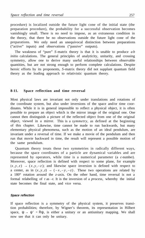
Space reflection and time reversal 257
procedure) is localized outside the future light cone of the initial state (thepreparation procedure), the probability for a successful observation becomesvanishingly small. There is no need to impose, as an extraneous condition inthe theory, that there be no observations outside the future light cone of thepreparations. We only need an unequivocal distinction between preparations(“active” inputs) and observations (“passive” outputs).
The weakness of “pure” S -matrix theory is that it is unable to produce a binitio calculations. The general principles of analyticity, unitarity, and crossingsymmetry, allow one to derive many useful relationships between observablequantities, but are not strong enough to perform complete calculations. Despiteheroic efforts by its proponents, S-matrix theory did not supplant quantum fieldtheory as the leading approach to relativistic quantum theory.
Space reflection and time reversal8-11.
Most physical laws are invariant not only under translations and rotations ofthe coordinate system, but also under inversions of the space and/or time coor-dinates. While it is in general impossible to reflect a physical object, it is oftenpossible to prepare an object which is the mirror image of the original one. Onecannot then distinguish a picture of the reflected object from one of the originalobject, viewed in a mirror. This is a symmetry, as defined at the beginningof this chapter. Likewise, time cannot be made to run backwards, but manyelementary physical phenomena, such as the motion of an ideal pendulum, areinvariant under a reversal of time. If we make a movie of the pendulum and thenrun that movie backward in time, the result will represent a possible motion ofthe same pendulum.
Quantum theory treats these two symmetries in radically different ways,because the space coordinates of a particle are dynamical variables and arerepresented by operators, while time is a numerical parameter (a c-number).Moreover, space reflection is defined with respect to some plane, for example(x , y , z ) → ( x , y , – z ); and likewise space inversion is defined with respect toa center, as in (x , y , z) → ( – x , – y , – z) . These two operations are related bya 180° rotation around the z-axis. On the other hand, time reversal is not aformal relabelling of t as –t. It is the inversion of a process, whereby the initialstate becomes the final state, and vice versa.
Space reflection
If space reflection is a symmetry of the physical system, it preserves transi-tion probabilities; therefore, by Wigner’s theorem, its representation in Hilbertspace, ψ → ψ' = Rψ, is either a unitary or an antiunitary mapping. We shallnow see that it can only be unitary.

258 Spacetime Symmetries
The simplest way of representing a reflection is ψ' (x) = ψ ( –x ). This is aunitary transformation, because
(8.159)
Exercise 8.38 Show that if p = then .
We now easily see that the antiunitary transformation law ψ' (x) =would not be acceptable. It would leave ⟨p⟩ invariant, while we expect the signof ⟨ p⟩ to change, as in the preceding exercise. Moreover, an energy eigenstate,ψ = f ( x ), would become f (– x), with the opposite sign of energy.This is impossible if the Hamiltonian has a semi-infinite spectrum, boundedbelow (that is, if the system has a ground state).
Another unitary transformation, more general than the one in Eq. (8.159), isRψ (x) = e iαψ ( – x ), where α is an arbitrary phase. If we want two consecutivereflections to restore the original state, we must have ei α = ± 1. The ± signis a characteristic property of the particle whose state is reflected. This sign iscalled the intrinsic parity of that particle, and its effect becomes manifest inreactions where particles of that type are produced or absorbed.
Exercise 8.39 Show that is invariant under inversions.
Time reversal
Time reversal (for which a better name would have been motion reversal ) isdefined as follows. Consider the unitary evolution
(8.80)
If the dynamical properties of the system are symmetric under time reversal,there exists a mapping v (t j ) → v ( t j
T ) such that the same unitary operatorU( t2 , t 1), which transforms v( t1 ) into v( t2 ), also transforms vT( t2 ) into v T( t1) :
(8.160)
We then have, from Eqs. (8.80) and (8.160),
(8.161)
Since these two inner products are antilinear in v(t1 ) and v (t 2 ) it follows thatvT( t j ) must be an antilinear function of v( t j ). Therefore time reversal is anantiunitary mapping.
This result was first derived by Wigner. 31 There have been attempts to definetime reversal in other ways,32,33 but Wigner’s definition is the one which is nowuniversally adopted.
31 E. P. Wigner, Göttinger Nachrichten, Math.-Phys. 31 (1932) 546.32 G. Racah, Nuovo Cimento 14 (1937) 322.33 J. Schwinger, Phys. Rev. 82 (1951) 914.

Bibliography 259
Exercise 8.40 Show that ⟨ p⟩ and ⟨ J ⟩ change sign under time reversal.
Another important symmetry is charge conjugation (a better name wouldhave been: particle-antiparticle exchange). A fundamental theorem of quantumfield theory states that any Lorentz invariant local field theory must be invariantunder the combined operations of space reflection, time reversal, and chargeconjugation. 34,35
8-12. Bibliography
More details on these topics can be found in specialized books, such as
F. R. Halpern, Special Relativity and Quantum Mechanics, Prentice-Hall,Englewood Cliffs (1968).
J. J. Sakurai, Invariance Principles and Elementary Particles, PrincetonUniv. Press (1964).
P. Ramond, Field Theory: A Modern Primer, Addison-Wesley, RedwoodCity (1989).
J. Wess and J. Barger, Supersymmetry and Supergravity, Princeton Univ.Press (1983).
Supersymmetry is an extension of relativistic spacetime symmetry, which incorpo-rates internal properties of particles. It allows bosons and fermions to appear in thesame supermultiplet representation.
Recommended reading
E. Wigner, “On the unitary representations of the inhomogeneous Lorentzgroup.” Ann. Math. 40 (1939) 149 [reprinted in Nucl. Phys. B (Proc. Suppl.)6 (1989) 9].
P. A. M. Dirac, “Forms of relativistic dynamics,” Rev. Mod. Phys. 21 (1949)392; “The conditions for a quantum field theory to be relativistic,” ibid. 3 4(1962) 592.
L. L. Foldy, “Synthesis of covariant particle equations,” Phys. Rev. 1 0 2(1956) 568.
R. Peierls, “Spontaneously broken symmetries,” J. Phys. A 24 (1991) 5273.
S. N. Mosley and J. E. G. Farina, “Quantum mechanics on the light cone:I. the spin zero case; II. the spin 1 case,” J. Phys. A 25 (1992) 4673, 4687.2–
34 G. Lüders, Ann. Phys. (NY) 2 (1957) 1.35 R. Jost, Helv. Phys. Acta 30 (1957) 409.

Chapter 9
Information and Thermodynamics
9-1. Entropy
Let us perform a quantum test on a physical system that was prepared in aknown way. Prior to the test, we can only predict probabilities for the possibleoutcomes. As the test is performed, one of these outcomes materializes, and wehave a certainty. A quantitative measure for the average amount of informationthat we expect to gain in this test can be defined as follows. Let p1 , . . . , p N bethe known probabilities of the various outcomes of the test that we intend toperform. Namely, if we imagine the same test applied to n identically preparedsystems, and if n is a large number, we expect about n j = n pj outcomes oftype j. From our knowledge of the preparation of the physical systems, we canpredict the relative frequencies of these outcomes, but not the order in whichindividual outcomes occur (as for example in Fig. 1.3, page 6). The number ofdifferent possibilities to arrange these n outcomes is n !/(n1 !n2!...). If n → ∞,all the n j are large and we have, by Stirling’s approximation,
(9.1)
The expression
(9.2)
is called the entropy of the probability distribution p1 , . . . , p N . It is a measureof our ignorance, prior to the test.
It is easy to see that S is maximum when all the pj are equal to 1/N. I n
order to avoid dealing with the constraint = 1, let us rewrite (9.2) as
(9.3)
260

Entropy 261
where pN is defined by
(9.4)
and all the other p j are considered as independent variables. We obtain
(9.5)
which vanishes when pk = p N = 1 / N. This is the only extremum of S.In general, the entropy S depends not only on the preparation process, but
also on the choice of the test with respect to which the probabilities pk are
preparation is called a random mixture (see Postulate C, page 31), and it isrepresented by the density matrix
(9.6)
For example, a photon coming from a thermal source is called “unpolarized,”to say that, in any unbiased polarization test, both outcomes are equally likely.
The other extreme is a pure state, with ρ² = ρ , as in Eq. (3.80), page 73.This relation implies the existence of a vector v such that
(9.7)
A pure state as in Eq. (9.7) corresponds to the maximal amount of informationwhich can be supplied on the preparation of a quantum system (Postulate A,page 30). Intermediate cases, as in Eq. (3.78), page 73, correspond to partialinformation on the preparation of a state.
Exercise 9.1 Photons are prepared by a process that has a 70% probabilityof producing right handed circular polarization, and a 30% probability of pro-ducing left handed circular polarization. What is the entropy of these photonsin a test for circular polarization? In a test for linear polarization? Ans.:0.61086 and 0.69315, respectively.
Exercise 9.2 Photons are prepared by a process that has a 70% probabilityof producing right handed circular polarization, and a 30% probability of pro-ducing them linearly polarized in the x direction. What is the entropy of thesephotons in a test for circular polarization? In a test for linear polarization inthe x direction? Ans.: 0.42271 and 0.64745, respectively.
The notion of entropy originally arose in classical thermodynamics and waslater introduced in information theory by Shannon.¹ It will be shown laterin this chapter that there is a close relationship between these two definitions
¹ C. E. Shannonon, Bell Syst. Tech. J. 27 (1948) 379, 623.
defined. If for every test we have maximal ignorance, namely pk = 1/ N, t he

262 Information and Thermodynamics
of entropy. In particular, the thermodynamic arrow of time which arises inirreversible phenomena is equivalent to the asymmetry between past and futurewhich is intrinsic in the processing of information.
Physicists usually include in the definition of entropy an extra factor equalto Boltzmann’s constant. Information theorists use logarithms with base 2. Inthe latter case, the unit of entropy (or of information) is called a bit ( f romabbreviation of binary digit).
Concave functions
An important property of entropy is that S (p) is a concave function of itsarguments p l , . . . , pN . This means that for any two probability distributions
and , and for any λ such that 0 ≤ λ ≤ 1, we have
(9.8)
The physical meaning of this inequality is that mixing different probabilitydistributions can only increase uniformity. The proof of (9.8) follows from
(9.9)
which is a sufficient condition for a function to be concave.² Moreover, thissecond derivative can vanish only if every
Exercise 9.3 Prove by induction that if λµ > 0 and = 1, and alsop µ j ≥ 0 and = 1, then
(9.10)
Suppose that the properties of a quantum system are specified by givingthe probabilities pm for the outcomes of some maximal test, T, which can beperformed on that system. The entropy of this probability distribution is ameasure of our ignorance of the actual result of test T. It will now be provedthat this entropy can never decrease if we elect to perform a different maximaltest. That other test may be performed either instead of test T, or after it, iftest T is repeatable.
Indeed, if the probabilities for test T are pm , those for a subsequent test are, where Pµ m is the doubly stochastic matrix defined in Sect. 2-4.
The new entropy thus is³
(9.11)
² R. Courant, Differential and Integral Calculus, Interscience, New York (1936) vol. II, p. 326.³ This inequality holds not only for entropy, but for any concave function. See G. H. Hardy,
J. E. Littlewood, and G. Pólya, Inequalities, Cambridge Univ. Press (1952) p. 89.

Entropy 263
The above inequality can be proved from4
(9.12)
where we used = 1. Since log x ≥ 1 – x –1 (with equality holding if,and only if, x = l), it follows that
(9.13)
where the equality sign holds if, and only if, Pµ m is a permutation matrix, sothat the sets pm and p'µ are identical.
You may find it paradoxical that no test whatsoever can decrease our igno-rance. To avoid a possible misunderstanding, I emphasize that the probabilitiesp'µ are those which are predicted before the test (after the test, there are noprobabilities—there are definite results). These p'µ always have a more uniformdistibution than the probabilities pm that were originally given (more precisely,they cannot have a less uniform distribution). Further consecutive tests canonly further increase the entropy: the more we intend to test, the less we canpredict what will be the final outcome. We can of course perform a selectionafter a test, and thereby acquire a perfect knowledge of the new state. Thisselection, however, amounts to preparing a new state, and erases all knowledgeof the original state.
Entropy of a preparation
After a given preparation whose result is represented by a density matrix ρ,different tests correspond to different sets of probabilities pm , and therefore todifferent entropies. Let us define the entropy of a preparation as the lowest valuethat can be reached by the expression (9.2) for any complete test performed afterthat preparation. It will now be shown that the optimal test, which minimizesS in Eq. (9.2), is the one that corresponds to the orthonormal basis vµ formedby the eigenvectors of the density matrix ρ:
(9.14)
In that basis, ρ is diagonal. The eigenvalues wµ satisfy
and (9.15)
Recall now that Postulate K (page 76) asserts that the density matrix ρcompletely specifies the statistical properties of an ensemble of physical systems
4 E. T. Jaynes, Phys. Rev. 108 (1957) 171.

264 Information and Thermodynamics
that were subjected to a given preparation. All the statistical predictions thatcan be obtained from ⟨ A⟩ = Tr(ρA) are the same as if we had an ordinary(classical) mixture, with a fraction wµ of the systems being with certainty instate v µ . Therefore, if the maximal test corresponding to the basis vµ is designedso as to be repeatable, the probabilities wµ remain unchanged 5 and thereforethe entropy S remains constant. The choice of any other test can only increasethe entropy, as we have just seen. This proves that the optimal test, whichminimizes the entropy, is the one corresponding to the basis vµ that diagonalizesthe density matrix. The entropy of a preparation can therefore be written as
(9.16)
where the logarithm of an operator is defined by Eq. (3.58), page 68.
Exercise 9.4 What are the eigenvalues and eigenvectors of ρ in Exercise 9.2?What is the physical meaning of these eigenvectors? What is the entropy of thepreparation? Ans.: 0.36535.
Composite systems
The entropic properties of composite systems obey numerous inequalities.6
Some of them are proved below, and will be used later in this chapter. First,we need the following lemma:
Let vm and e µ be two orthonormal bases for the same physical system,and let a n d be two different density matrices.Their relative entropy S(σ ρ) is defined by
(9.17)
Let us evaluate this expression in the vm basis, where ρ is diagonal. The diagonalelements of log σ are
(9.18)
The matrix Pµ m = is doubly stochastic, and we have, as in the proofof Eq. (9.12),
(9.19)
with equality holding if, and only if, σ = ρ. Note that the above proof holdseven though ωµ is not equal to
5 Here, one would be tempted to say that the state of each system remains unchanged.However, this claim is not experimentally verifiable. Only the probabilities wµ can be shownto remain constant.
6 A. Wehrl, Rev. Mod. Phys. 50 (1978) 221.

Entropy 265
Consider now a composite system, with density matrix ρm µ ,nv (double indiceshave the same meaning as in Chapter 5). The reduced density matrices of thetwo subsystems are
and (9.20)
It will now be shown that
(9.21)
This inequality, called subadditivity,6 means that a pair of correlated systemsinvolves more information than the two systems considered separately.
Exercise 9.5 Verify subadditivity for two spin j particles in a singlet state.Ans.: Eq. (9.21) becomes 0 < log(2j + 1).
In order to prove the inequality (9.21), we first note that
(9.22)
because
(9.23)
where w m , ω µ , and Wmµ = w m ω are the eigenvalues of ρ1 , ρ2 , and ρ1 ⊗ ρ2 ,respectively. Consider now the relative entropy
(9.24)
This is a nonnegative quantity, by virtue of (9.19). On the other hand, we have
(9.25)
and likewise for Tr (ρ log ρ2 ). The subadditive property (9.21) readily follows.It can also be shown that7
(9.26)
so that S (ρ), S (ρ1), and S (ρ2) obey a triangle inequality.
7 H. Araki and E. H. Lieb Comm. Math. Phys. 18 (1970) 160.
µ

266 Information and Thermodynamics
Information erasure
We can now see why information processing is associated with an irreversiblearrow of time. There is nothing intrinsically irreversible in the logic of the com-puting process. However, we must initially load data into a memory. Assumefor simplicity that the memory elements are built in such a way that the binarydigits 1 and 0 are represented by orthogonal states, u and v, respectively. 8
Further assume that the last computation that has been done has left thesememory elements in states u and v with equal probabilities. Therefore the stateof each memory element is represented by a density matrix, , and itsentropy is log 2.
We must first reset each memory element to a standard state, such as v ,before we can start the computation. Such an erasure or overwriting of onebit of information transfers at least one bit of entropy to the environment,9
because no unitary evolution can transform the mixed state into apure state v v †. The only way of resetting the memory to zero is to couple itwith a reservoir, which initially is in a known pure state w, and let the combinedsystem follow a unitary evolution,
(9.27)
This sets the memory element in a standard state, as we wished, but meanwhileone bit of entropy has been dumped into the reservoir which cannot be usedagain since it now is in a mixed state.
Exercise 9.6 Write explicitly the unitary operator U which produces
and (9.28)
where x is orthogonal to w.
9-2. Thermodynamic equilibrium
A Boltzmann distribution (also called Gibbs state) is one whose density matrix ρhas eigenvectors which coincide with those of the Hamiltonian, and has eigen-values w µ related to the energy levels Eµ by
(9.29)
The sum
(9.30)
8 A more realistic assumption would be the use of density matrices, rather than pure states.This would bring no change in the conclusions.
9 R. Landauer, IBM J. Res. Dev. 5 (1961) 183.

Thermodynamic equilibrium 267
is called the partition function of the system. Preparations satisfying Eq. (9.29)are said to be in thermodynamic equilibrium at temperature T = 1/β. (It isconvenient to use energy units for the temperature, so that Boltzmann’s con-stant is unity.) A random mixture satisfying Postulate C, page 31, correspondsto β = 0, namely thermal equilibrium at infinite temperature.
It readily follows from (9.29) and (9.30) that the mean energy is
(9.31)
Exercise 9.7 Show that a Gibbs state has the maximal entropy compatiblewith a given value of ⟨ E⟩.
Exercise 9.8 Show that
In a process slow enough to preserve thermodynamic equilibrium, we have
(9.32)
The term is due to a shift of the energy levels caused by variationsof the external parameters. We call it the work performed on the system, while
(9.33)
is the heat transferred to the system (the effect of heat transfer is to change theprobabilities of occurrence of the various energy levels).
On the other hand, we have from (9.29)
(9.34)
where we have used . Comparing Eqs. (9.33) and (9.34), we obtain
(9.35)
which is the familiar thermodynamic definition of entropy.10 It should be keptin mind that this definition applies only to systems in thermal equilibrium,while the more general definition (9.2) is always valid.
We must now explain why it often happens that physical systems tend tothermal equilibrium. An isolated system certainly does not. If its densitymatrix is , each v µ evolves linearly, as , but thecoefficients wµ remain constant. Therefore the entropy given by Eq. (9.16) isconstant too. (The same is also true in classical statistical mechanics, wherethe entropy is defined by the Liouville density in phase space.) The following
10 F. Reif, Fundamentals of Statistical and Thermal Physics, McGraw-Hill, New York (1965)pp. 218–219.

268 Information and Thermodynamics
argument 11 shows that thermalization of a quantum system may result frommultiple collisions with other systems which already are in thermal equilibrium.
Collisions
In a collision of two quantum systems which are initially uncorrelated, thecombined density matrix evolves as
(9.36)
The total entropy, , remains constant under this unitarytransformation. However if we consider separately the final states of the twosubsystems after the collision, these are given by the reduced density matrices
and (9.37)
and we have, by virtue of the subadditivity inequality (9.21),
(9.38)
This growth of the total entropy is caused by the replacement whereby we “forget” the correlations that were created in the collision process.This entropy growth is not a dynamical process, and is solely due to the way theproblem is formulated. There is no mysterious time-asymmetry here: if we weregiven the final reduced density matrices (after the collision) and were asked forour best estimate of the initial uncorrelated density matrix, our answer wouldalso involve more entropy than the data supplied to us.
We shall write Eq. (9.38) as
(9.39)
In general, the symbol ∆ will denote the increment of a physical quantity, dueto a collision. For example, we have
(9.40)
by energy conservation.For a system in a Gibbs state (9.29), we have
(9.41)
If that system collides with another one, its final density matrix will not, ingeneral, be a Gibbs state, but we may still consider the quantity where β refers to the initial state, before the collision. We then have
11 M. H. Partovi, Phys. Letters A 137 (1989) 440.

Thermodynamic equilibrium 269
(9.42)
This expression is the relative entropy S(ρ|ρ') which was defined by Eq. (9.17)and is nonnegative, as we have seen.
Approach to equilibrium
Consider a collision of system a, initially in any state, with system b, which isinitially in a Gibbs state at temperature β – l. We have, from Eq. (9.42),
(9.43)
Combining this result with Eqs. (9.39) and (9.40), we obtain
(9.44)
Therefore if system a, initially in any state, undergoes multiple collisionswith other systems, all initially in Gibbs states at the same temperature β– 1,the expression never decreases, and it will eventually approach alimiting value. If there are no selection rules (that is, if there are no conservationlaws inhibiting transitions between some of the energy levels Eµ of system a)this limiting value is the one which maximizes
(9.45)
subject to the constraint Using the method of Lagrange multipliers,it is easily found that the solution is the Gibbs state (9.29).
Zeroth law of thermodynamics
Consider now an interaction of two systems, a and b, initially in Gibbs statesat different temperatures and From Eq. (9.43), we have
(9.46)
and likewise
(9.47)
Together with Eqs. (9.39) and (9.40), this gives
(9.48)
which means that heat flows from the system having a higher temperature tothe system with the lower temperature.

270 Information and Thermodynamics
Second law of thermodynamics
Finally, consider multiple interactions of system a with an array of systems bn ,which initially are in Gibbs states at various temperatures . At each step,we have, from Eq. (9.44),
(9.49)
where δQ n is the energy transferred to the n -th reservoir and converted intoheat. In a cyclic process, the initial and final states of system a are identical,so that whence The total entropyof the reservoirs must not decrease while system a undergoes a cyclic process.
9-3. Ideal quantum gas
It will now be shown that the quantum entropy (9.16) is genuine entropy, fullyequivalent to that of standard thermodynamics. Let us first recall the proofthat the entropy of a mixture of dilute, inert, ideal gases is
(9.50)
where is the total number of gas molecules, and is theconcentration of the j-th species. The derivation of Eq. (9.50) is given belowfor the case of two different species, It assumes the existence of semipermeablemembranes which are transparent to molecules of type j, and opaque to allothers. These membranes are used as pistons in an ideal frictionless engineimmersed in an isothermal bath at temperature T, as sketched in Fig. 9-1.
Fig. 9.1. Ideal engine used to separate gases A (to the left) and B (to the right).The vertically and horizontally hatched semipermeable pistons are transparent togases A and B, respectively. The mechanical work supplied in order to transformthe initial state into the final state is released as heat into the thermal bath.

Ideal quantum gas 271
The first step of the separation is a motion toward the right of the pair ofpistons that are connected by a rigid rod. Gas A exerts no pressure on the leftpiston (which is transparent to it) and gas B exerts the same pressure on bothpistons. Therefore no work is needed for this reversible separation. Then, eachgas is isothermally compressed to reduce its volume by a factor cj , so that thefinal total volume is the same as the initial one. The isothermal work neededfor compressing the j-th ideal gas is
(9.51)
This work is released into the reservoir where it is converted into heat. Sincethe entire process is macroscopically reversible, the total entropy is conserved.Therefore the mixing entropy, in the initial state, is given by Eq. (9.50). Andvice versa, TS is the maximum amount of heat convertible into mechanicalwork by isothermal mixing of ideal gases. (Recall that the name heat is givento the energy randomly distributed among the many degrees of freedom of thereservoir, for which we gave up the possibility of a detailed description.)
The quantum definition of entropy closely parallels the above argument. Italso assumes the existence of semipermeable membranes which can be used forperforming quantum tests. These membranes separate orthogonal states withperfect efficiency. The fundamental problem here is whether it is legitimate totreat quantum states in the same way as varieties of classical ideal gases.
This issue was clarified by Einstein12 in the early days of the “old” quantumtheory, as follows: Consider an ensemble of quantum systems, each one enclosedin a large impenetrable box, so as to prevent any interaction between them.These boxes are enclosed in an even larger container, where they behave as anideal gas, because each box is so massive that classical mechanics is valid for itsmotion (i.e., there is no need of Bohr-Sommerfeld quantization rules—rememberthat Einstein’s argument was presented in 1914). The container itself has idealwalls and pistons which may be, according to our needs, perfectly conducting,or perfectly insulating, or with properties equivalent to those of semipermeablemembranes. The latter are endowed with automatic devices able to peek insidethe boxes and to test the state of the quantum systems enclosed therein. Theentire machine can then function like the one in Fig. 9.1.
Similar assumptions were later used by von Neumann13 who emphasized thatthe practical infeasibility of Einstein’s fantastic contraption did not impair itsdemonstrative power: “In the sense of phenomenological thermodynamics, eachconceivable process constitutes valid evidence, provided that it does not conflictwith the two fundamental laws of thermodynamics.” von Neumann showed thatthe mixing entropy (9.50) could be written as where ρ isthe density matrix representing the state of each quantum system. The cj ofEq. (9.50) are analogous to the eigenvalues of ρ.
12 A. Einstein, Verh. Deut. Phys. Gesell. 16 (1914) 820.13J. von Neumann, Mathematische Grundlagen der Quantenmechanik, Springer, Berlin
(1932) p. 191 [t ransl. by E. T. Beyer: Mathematical Foundations of Quantum Mechanics,Princeton Univ. Press (1955) p. 359].

272 Information and Thermodynamics
Quantization of Einstein’s state selector
This hybrid classical-quantal reasoning is not satisfactory, because there is noconsistent dynamical formalism for interacting classical and quantum systems. Ishall now outline a genuinely quanta1 proof of the equivalence of von Neumann’sentropy (9.16) to the ordinary entropy of classical thermodynamics.
Let q denote collectively all the internal degrees of freedom of a quantumsystem, and let R denote its center of mass. The components of R have thesame role as the coordinates of Einstein’s impenetrable classical boxes, but theyare quantum variables. The Hamiltonian of the quantum system is
(9.52)
where H0 involves only the internal variables, P is the momentum conjugateto R, and M is the mass of the system. At this stage, there is no interactionbetween the internal degrees of freedom q and the translatory ones, R and P.
We now introduce Einstein’s large container, which also plays the role of athermal reservoir. As is customary in thermodynamics, the properties of thiscontainer are extremely idealized. Its degrees of freedom fall into two classes: asmall number of macrovariables collectively denoted by X (position of the centerof mass, spatial orientation, location of the pistons, etc.) and a huge numberof microvariables, denoted by x, which describe the atomic structure of thecontainer (the symbols X and x also denote momenta). The idealization hereis the absence of “mesovariables,” such as collective excitations which involve103 or 10 9 atoms, and are neither microscopic nor macroscopic. Such an idealcontainer can exist only in our imagination. Nevertheless, as long as it does notviolate known laws of physics, it is a perfectly legitimate tool for discoveringadditional laws (see above quote from von Neumann’s book).
The characteristic property of the macrovariables is that, if their observablevalues are initially sharp, namely they remain sharp during theentire dynamical evolution. This property does not hold for microvariables suchas the positions and momenta of individual molecules, whose values quicklyacquire a large dispersion, because of multiple collisions. The molecules alsocollide with the container, but each collision has a very small effect on thelatter. Only the total effect is noticeable: it is the pressure exerted on the wallsand pistons, and the fluctuations of that pressure are small if the container isvery large and there are many quantum systems enclosed in it.
The Heisenberg equations of motion for x and X have the form
(9.53)
and
(9.54)
where Fext (a c -number) is due to external agents under the direct control ofthe experimenter who is actuating the pistons, opening and closing valves, etc.

Ideal quantum gas 273
Taking average values in the last equation, we obtain
(9.55)
Thanks to the small dispersion of the X variables, it is possible to replace, onthe right hand sides of (9.53) and (9.55), X by ⟨X ⟩ (or, if you prefer, by ⟨ X ⟩ 1 ) ,and to consider X⟨ ⟩ as a classical variable, that we shall write simply as X. W eknow that it is in general inconsistent to mix classical and quantum dynamicalvariables; however, no inconsistency arises if we treat the X variables as merenumerical parameters, having a prescribed dependence on time.
We further assume that these X parameters have a very slow motion, sothat the microvariables are at every instant in thermal equilibrium. They havea Gibbs distribution at temperature β–l :
(9.56)
where H c is the Hamiltonian of the container, which depends on x and on thenumerical parameters X. It is thanks to this thermal equilibrium that thedispersion of the X variables always remains small.
Finally, we introduce an interaction between our quantum system and thecontainer in which it is enclosed. This interaction causes multiple scatteringsof the quantum system with the walls and pistons. It is essential that ∆ H, theenergy spread of the quantum system, far exceeds the average level spacing ofthe energy spectrum of the macroscopic container, so that the quantum systemdoes not feel the discreteness of the spectrum of the container.
Two cases must now be distinguished, depending on whether the containerhas semipermeable partitions which interact with the internal variables of thequantum system, or only ordinary walls and pistons. In the latter case, theinteraction term in the Hamiltonian involves the macrovariables X (consideredas classical parameters), the microvariables x (quantized), and the positionvariables R and P of the quantum system, but not its internal variables q .The evolution of the latter thus is completely disjoint from that of the othervariables. We can now apply the results of the preceding section. The finalvalue of for the R and P variables corresponds to a Gibbs state atthe same temperature β —1 as the reservoir. That is, an ensemble of quantumsystems described by the Hamiltonian (9.52) has the same statistical propertiesas a classical ideal gas of free particles of mass M. In particular, it exertsexactly the same pressure on the walls of the container.
Selection of orthogonal states
The situation becomes more interesting if semipermeable partitions are intro-duced. The latter may be described by an interaction term involving q, R, P,and X. Recall that the classical parameters X, which include the positions ofthe movable partitions, are prescribed functions of time. Their time dependence

274 Information and Thermodynamics
must be extremely slow on time scales relevant to the x, R, and P variables, sothat the latter always are in thermal equilibrium.
If we add to the right hand side of (9.52) a term H int(q, R, X ), its effect willbe to generate an entangled state, where the variables q and R are correlated.As an extremely simplified model, take a one dimensional container. Particleswith spin up can be concentrated on one side of a partition located at positionX, and particles with spin down on the other side, by means of an interaction
(9.57)
where V 0 and K are large constants, and the symbol “tanh” stands for anysmoothed step function. This interaction produces a force acting onthe quantum system when its position is in the vicinity of X, the location ofthe semipermeable partition. The result is like a Stern-Gerlach experiment.Particles with opposite values of σz are accelerated in opposite directions. Thefinal wave function (in the coordinate representation) is the sum of two terms.In each one of them, has the same sign as
Exercise 9.9 Write an interaction which sorts out different eigenvalues of anyoperator A into different regions of a three dimensional container.
This simple abstract model demonstrates that it is possible, at least in theory,to dispatch into different regions of the R-space quantum systems in orthogonalstates. They behave exactly as if they were a mixture of classical ideal gasesof different types. Therefore there should be no doubt that von Neumann’sentropy (9.16) is equivalent to the entropy of classical thermodynamics. (Thisstatement must be understood with the same vague meaning as when we saythat the quantum notions of energy, momentum, angular momentum, etc., areequivalent to the classical notions bearing the same names.)
Free energy of a pure state
On the other hand, there also are circumstances under which an ensemble ofquantum systems displays thermodynamic properties quite different from thoseof a mixture of classical ideal gases. This is due to the existence of n o n -orthogonal states, which are essentially nonclassical. These states are partlyalike—neither identical, nor completely different from one another. They enableus to convert in a continuous way any quantum state into any other quantumstate, as shown below (for a concrete example, see Exercise 1.1, page 7).
Exercise 9.10 Let v and w be two orthogonal states of a quantum system.Show that with real λ , is a unitary matrix whichrotates the subspace spanned by v and w :
(9.58)

Some impossible processes 275
In the following discussion, it will be assumed that any unitary evolution, suchas the one in Eq. (9.58), can in principle be realized in the laboratory. It isan isentropic process, and any energy that has to be supplied can be reversiblyrecaptured (or, if you prefer, you can put the system in an environment suchthat v and w become degenerate energy eigenstates).
We shall now see that an ensemble of n quantum systems in any pure statecan extract energy from a thermal reservoir at temperature T. Indeed, takeone half of these systems, and reversibly rotate their pure state into an ortho-gonal state, as in Eq. (9.58). Then, mix these two subensembles, isothermallyand reversibly. This extracts an energy nT log 2 from the thermal reservoir.More generally, if the quantum systems used for this process have N orthogonalstates, you can divide an ensemble prepared in a pure state into N identicalsubensembles, reversibly rotate N – 1 of them into mutually orthogonal states,and finally mix them together, thereby extracting an energy nT log N from thethermal reservoir.
9-4. Some impossible processes
In the preceding section, we examined conceptual processes which would havebeen exceedingly difficult to realize in practice, but did not violate any funda-mental physical principle. I shall now describe truly impossible tasks, and showthat there is a close relationship between dynamical evolutions which violatesome fundamental principle of quantum theory (such as unitarity) and thosewhich are forbidden by the second law of thermodynamics.
It thus appears that thermodynamics imposes severe constraints on the choiceof fundamental axioms for quantum theory. However, this claim heavily relieson the equivalence of von Neumann’s entropy to the ordinary entropy of thermo-dynamics. The proof of this equivalence assumes the validity of Hamiltoniandynamics (in order to derive the existence of thermal equilibrium), and theremay be a logical error here, known as petitio principii: we invoke Hamiltoniandynamics in order to prove some theorems, and then we claim as a corollaryof these theorems that non-Hamiltonian dynamics is inconsistent. Thus, thefinal conclusion to be drawn from this discussion is that if the integrity of theaxiomatic structure of quantum theory is not strictly respected, then everyaspect of the theory must be reconsidered.
Selection of non-orthogonal states
The interaction in Eq. (9.57) and its multidimensional generalizations allow usto distinguish different eigenvalues of Hermitian operators, which correspondto orthogonal states of a quantum system. Can there be more general tests?Imagine that a wily inventor claims having produced semipermeable partitionswhich unambiguously distinguish non-orthogonal states. He can thereby convert

276 Information and Thermodynamics
into work an unlimited amount of heat extracted from an isothermal reservoir,as shown below. Will you invest your money in this new technology?
Before we examine how this marvellous invention works, let us first noticethat such a process violates the completeness postulate K , which asserts thata density matrix ρ is a complete specification of all the physical properties ofan ensemble (see page 76). Indeed, let P 1 and P 2 represent two pure statesof a quantum system, and let ρ0 be the initial state of an instrument builtfor separating them. An interaction with a properly constructed instrumentgenerates the following dynamical evolutions:
and (9.59)
where the final states ρ1 and ρ2 are orthogonal (that is, ρ1 ρ2 = O ). For example,ρ1 and ρ 2 may be located in different regions of space.14 If the initial state ofthe quantum system is a mixture, –1 (P1 + P2), the effect of the separator is
2
(9.60)
This relation follows from Postulate K, because the representation of a statisticalensemble by the expression –1 ( P
2 1 + P 2) means that this ensemble behaves as if50% of its elements are in state P1 and 50% in state P 2. There is no need hereto assume linearity, because there are no interference effects between the twocomponents if the initial state is a mixture.
The dynamical process represented by Eq. (9.60) is a separation of the P1
and P 2 components of the mixture, such that each one ends up correlated toa different final state of the instrument. Taking the squares of both sides ofEq. (9.60), we obtain, apart from a factor –1 :4
(9.61)
where use was made of P j2
1 ≡ Pj , and ρ ρ2 = O . Subtracting from Eq. (9.61)the squares of Eqs. (9.59) then gives P1P2 + P2P1 = O . Therefore Eq. (9.60) isconsistent if, and only if, states P1 and P2 are orthogonal.
Consider now the cyclic process illustrated in Fig. 9.2, which involves twonon-orthogonal photon states. Suppose that there are n photons in the vessel.One half of them are prepared with vertical linear polarization, and the otherhalf with a linear polarization at 45° from the vertical. Initially, in state (a) ,they occupy two chambers with equal volumes. The first step of the cyclicprocess is an isothermal expansion, doubling these volumes, as shown in (b) .This expansion supplies an amount of work nT log 2, where T is the temperatureof the reservoir. At that stage, the impenetrable partitions separating the twophoton gases are replaced by semipermeable membranes, as in Fig. 9.1. These
14 It is always possible to consider ρ0 as a pure state, which satisfies ρ02 = ρ 0, by introducing
an auxiliary Hilbert space, as shown in Exercise 5.10. However, that mock Hilbert space doesnot participate in the dynamical evolution, and one cannot impose that ρ1 and ρ 2 be purestates too.

Some impossible processes 277
membranes, however, have the extraordinary ability of selecting non-orthogonalstates: One of them is transparent to vertically polarized photons, and reflectsthose with polarization at 45° from the vertical; the other membrane has theopposite properties. A double frictionless piston, like the one in Fig. 9.1, canthus bring the engine to state (c), without expenditure of work or heat transfer.We have thereby obtained a mixture of the two polarization states, with densitymatrix
(9.62)
The eigenvalues of ρ are 0.854 ( corresponding to photons polarized at 22.5°from the vertical) and 0.146 (for the orthogonal polarization).
Fig. 9.2. This cyclic process extracts heat from an isothermalreservoir and converts it into work, by using a hypotheticalsemipermeable partition which separates non-orthogonal photonstates. Double arrows indicate the polarizations of the photons.
We now replace the “magic” membranes by ordinary ones, which reversiblyseparate these two orthogonal polarization states, and yield state (d ). The nextstep is an isothermal compression, leading to state (e) where both chambershave the same pressure and the same total volume as those in state (a). Thisisothermal compression requires an expenditure of work
–nT (0.146 log 0.146 + 0.854 log 0.854) = 0.416 nT, (9.63)
which is released as heat into the reservoir. This work is less than nTlog2,the amount that was gained in the isothermal expansion from (a) to ( b). Thenet gain is 0.277 nT. Finally, no work is involved in returning from (e) to (a),by suitable rotations of polarization vectors, as in Eq. (9.58). We have thusdemonstrated the existence of a closed cycle whereby an unlimited amount ofheat can be extracted from an isothermal reservoir and converted into work, inviolation of the second law of thermodynamics.
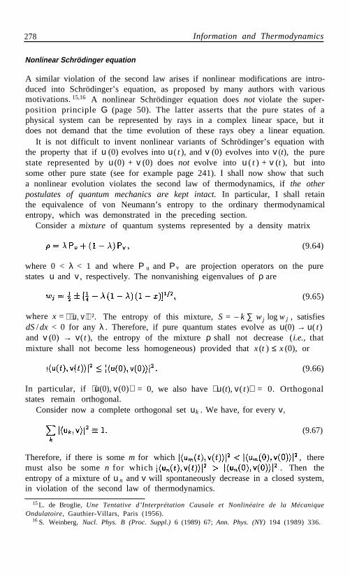
278 Information and Thermodynamics
Nonlinear Schrödinger equation
A similar violation of the second law arises if nonlinear modifications are intro-duced into Schrödinger’s equation, as proposed by many authors with variousmotivations. 15,16 A nonlinear Schrödinger equation does not violate the super-position principle G (page 50). The latter asserts that the pure states of aphysical system can be represented by rays in a complex linear space, but itdoes not demand that the time evolution of these rays obey a linear equation.
It is not difficult to invent nonlinear variants of Schrödinger’s equation withthe property that if u (0) evolves into u ( t ), and v (0) evolves into v (t), the purestate represented by u (0) + v (0) does not evolve into u ( t ) + v (t ), but intosome other pure state (see for example page 241). I shall now show that sucha nonlinear evolution violates the second law of thermodynamics, if the otherpostulates of quantum mechanics are kept intact. In particular, I shall retainthe equivalence of von Neumann’s entropy to the ordinary thermodynamicalentropy, which was demonstrated in the preceding section.
Consider a mixture of quantum systems represented by a density matrix
(9.64)
where 0 < λ < 1 and where P u and P v are projection operators on the purestates u and v , respectively. The nonvanishing eigenvalues of ρ are
(9.65)
where x = ⟨ u, v ⟩ ². The entropy of this mixture, S = – k ∑ w j log w j , satisfiesdS / dx < 0 for any λ . Therefore, if pure quantum states evolve as u(0) → u( t)and v (0) → v(t ), the entropy of the mixture ρ shall not decrease (i.e., thatmixture shall not become less homogeneous) provided that x (t ) ≤ x (0), or
(9.66)
In particular, if ⟨u(0), v(0)⟩ = 0, we also have ⟨ u(t), v( t )⟩ = 0. Orthogonalstates remain orthogonal.
Consider now a complete orthogonal set uk . We have, for every v,
(9.67)
Therefore, if there is some m for which , theremust also be some n for which . Then theentropy of a mixture of u n and v will spontaneously decrease in a closed system,in violation of the second law of thermodynamics.
15 L. de Broglie, Une Tentative d’Interprétation Causale et Nonlinéaire de la MécaniqueOndulatoire, Gauthier-Villars, Paris (1956).
16 S. Weinberg, Nucl. Phys. B (Proc. Suppl.) 6 (1989) 67; Ann. Phys. (NY) 194 (1989) 336.

Generalized quantum tests 279
To retain the second law, we must have forevery u and v . It then follows from Wigner’s theorem (Sect. 8-2) that, withan appropriate choice of phases, the mapping v(0) → v (t) is unitary (the anti-unitary alternative is ruled out by continuity). Schrödinger’s equation musttherefore be linear, if we retain the other postulates of quantum theory withoutany change.
No-cloning theorem
It was shown in Sect. 3-5 that, if we know that a large number of quantumsystems have been prepared identically, it is possible to determine their stateunambiguously by suitable quantum tests. On the other hand, we have just seenthat it is impossible to distinguish unambiguously non-orthogonal states of asingle system. Why can’t we overcome this difficulty by making many identicalreplicas of that system, just as we duplicate a letter with a photocopier?
Imagine that there is an amplifier, initially in a state Ψ , with the ability ofduplicating quantum systems prepared in an arbitrary state. That is,
( ? ) (9.68)
where Ψ' is the state of the amplifier after performing its duty. Likewise, for adifferent input state of the quantum system, we would have
(?) (9.69)
Take the inner product of these two equations. Unitarity implies that
(?) (9.70)
In this equation, we have 0 < ⟨ v,w ⟩ < 1 for suitable choices of v and w , andalso ⟨ Ψ , Ψ ⟩ ≡ 1. It follows that ⟨ Ψ' , Ψ" ⟩ ⟨ v,w⟩ = 1, which is impossible, because⟨Ψ ', Ψ" ⟩ ≤ 1. Therefore such an amplifier cannot exist. 17,18
9-5. Generalized quantum tests
The most efficient way of obtaining information about the state of a quantumsystem is not always a maximal test (as defined in Chapter 2). It is sometimespreferable to introduce an auxiliary quantum system, prepared in a standardstate, and to execute a combined quantum test on both systems together. Weshall now examine these indirect quantum tests, which actually are the mostcommon ones. The maximal tests that were considered until now are a conve-nient conceptual notion, but are seldom realized in practice.
17 W. K. Wootters and W. H. Zurek, Nature 299 (1982) 802.18 D. Dieks, Phys. Letters A 92 (1982) 271.

280 Information and Thermodynamics
Formulation of the problem
The classic treatise on the foundations of quantum theory is von Neumann’sbook. 13 Historically, this was the first rigorous presentation of a mathematicalformalism for quantum theory, with a consistent physical interpretation. Thebook had a disproportionate influence on quantum methodology. In particular,most subsequent investigations of the “quantum measurement problem” haverevolved around the determination of values of dynamical variables which haveclassical counterparts: positions, momenta, energies, etc. In von Neumann’sapproach, these dynamical variables (classically—functions of q and p) arerepresented by self-adjoint operators acting on H, the Hilbert space of quantumstates. Their spectrum corresponds to an orthogonal resolution of the identity,because the various outcomes of a quantum test are mutually exclusive, andtheir probabilities sum up to 1.
It was later realized that von Neumann’s theory of quantum measurementswas too narrow. It did not allow to ask simple questions referring to welldefined physical situations. As an example, suppose that a spin –1 particle is
2prepared in a pure state. Its wave function ψ satisfies σ·nψ = ψ, for some unitvector n. The state ψ is uniquely defined (up to an irrelevant phase) if n isgiven. The question “What is n?” has an obvious classical analog (“What is thedirection of the angular momentum?”). It is a legitimate way of inquiring aboutthe preparation of the system. That preparation is a macroscopic procedure,without any “quantum uncertainties.” However, n is not a quantum dynamicalvariable (a self-adjoint operator acting on H). The only “quantum observables”of a spin 1– particle are the components of σ and linear combinations thereof.
2The situation described above may occur in actual experiments. Polarized
neutrons are used as probes for measuring magnetic fields in condensed matter.We thus want to know the precession of the neutron’s magnetic moment. Thisis a well defined physical concept (represented in quantum theory by a unitaryoperator). Yet, there is no possibility of measuring this precession if only oneneutron is available. We need numerous, identically prepared neutrons in orderto obtain a good estimate of the precession angle. While this is not a seriousimpediment in experimental solid state physics, where you have an abundanceof identical particles, this may become one in other areas of physics, where onlya few quanta are available. For example, if we detect a small number of photonsfrom a distant star, how well can we determine their polarization? The mostefficient methods are not maximal tests, as we shall soon see.
Shannon’s entropy in quantum theory
The novel feature introduced by quantum theory is that preparations whichare macroscopically different can produce states which are not orthogonal, andtherefore cannot be distinguished unambiguously from each other. For instance,let the state of a spin 1– particle be prepared by selecting the upper beam in2a Stern-Gerlach experiment. We are given the choice of orienting the magnet

Generalized quantum tests 281
along direction n 1, or along direction n 2 . The corresponding quantum statesof the resulting beams, ψ1 and ψ 2 , are then given by σ σ · n j ψ j = ψ j . In general,these states are not orthogonal. Their overlap is
–
This expression is the probability that, following a preparation of state ψ , the1
question “Was the prepared state ψ ?” will be answered in the affirmative. The2
answer cannot be predicted with certainty. Once the spin 1 particle has been2severed from the macroscopic apparatus which prepared it, it does not carry thefull information relative to the preparation procedure. Some questions becomeambiguous, and only probabilities can be assigned to their answers.
This situation is radically different from the one prevailing in classical physics.Therefore quantum tests cannot be restricted to be mere imitations of classicalmeasurements, where all we want to know is the numerical value of a dynamicalvariable. More general procedures must be considered, which are adapted tothe rules of quantum theory.
–
Because of the peculiar properties of non-orthogonal states, it is necessaryto distinguish Shannon’s entropy, from von Neumann’s entropy,
For instance, our spin 1 particle may have N distinct preparation2procedures. If they are equally probable, Shannon’s entropy, log N, can bearbitrarily large. On the other hand, von Neumann’s entropy never exceedslog 2. Thus, paradoxically, we are less ignorant in quantum physics than inclassical physics: this is because there are fewer diferent ( i.e., orthogonal)questions that we are allowed to ask, and therefore there are fewer unknownanswers. To clearly distinguish these two kinds of entropies, Shannon’s entropywill henceforth be denoted by H (not S ) as is customary in information theory.(There is no risk of confusion here with the Hamiltonian.)
–
Exercise 9.11 Three different preparation procedures of a spin –1 particle2
are represented by the vectors and 1 If they are equally likely, the2
Shannon entropy is log 3, and the von Neumann entropy is log 2. Show that ifthere are n such particles, all prepared in the same way, the von Neumannentropy asymptotically tends to log 3 when n → ∞. Hint: Consider threereal unit vectors making equal angles: ⟨ ui , u ⟩ = c if i ≠ j. Show that thej
eigenvalues of are 1 – c, 1 – c, and 1 + 2c.
Quantum information gain
How well can we distinguish non-orthogonal states? Let us assume that thereare N different preparations, represented by known density matrices ρi , and letpi be the known a priori probability for preparation i. We further assume thatthe testing procedure may yield n different outcomes (in general n ≠ N). Ifwe have enough understanding of the physical processes involved in the test,we can compute the conditional probability Pµ i that preparation i shall yield
(9.71)

282 Information and Thermodynamics
result µ. Having found a particular result µ, we can then compute Qi µ , t h elikelihood (or a posteriori probability) for preparation i. It is given by Bayes’stheorem (see Appendix to Chapter 2):
(9.72)
where
(9.73)
is the a priori probability for occurrence of outcome µ.Before finding the result µ, we only knew the probabilities pi . Shannon’s
entropy, which is a measure of our ignorance, was – Σ pi log p i . After havingfound the result µ, we can compute the a posteriori probabilities Qi µ , and thenew entropy is
(9.74)
For some outcomes, H µ may be larger than the initial entropy, so that the resultof the test is to increase our uncertainty. Here is an amusing example, due toUffink: my key has a 90% chance to be in my pocket; if it is not, it may be ina hundred other places, with equal probabilities. The Shannon entropy thus is–0.9 log 0.9 – 0.1 log 0.001 = 0.7856. If I search in my pocket and I don’t findthe key in it, the Shannon entropy increases to – log 0.01 = 4.605. We thussee that Shannon’s entropy does not measure an objective ignorance level, butrather our subjective feeling of ignorance.
On the average, however, a quantum test reduces the Shannon entropy. Theaverage information gain is
(9.75)
We shall investigate the optimization of this information gain after we haveacquired the necessary mathematical tools.
Positive operator valued measures
The information gain (9.75) depends on the conditional probabilities Pµi forobtaining result µ when the system is prepared in state ρ i . The value of P µi isdetermined by the testing procedure. Consider the following model for a two-step operation: First, an auxiliary quantum system, called ancilla,19 is preparedin a known state ρ aux . The combined, uncorrelated state of the original quantumsystem and the ancilla is
19 C. W. Helstrom, Quantum Detection and Estimation Theory, Academic Press, New York(1976) pp. 74–83.

Generalized quantum tests 283
(9.76)
where italic and boldface indices refer to the original and auxiliary quantumsystems, respectively.
A maximal test is then performed in the combined Hilbert space. This isin principle always possible, by virtue of the strong superposition principle G
(page 54). That complete test is represented by an orthogonal resolution of theidentity. Different outcomes correspond to orthogonal projectors which satisfy
and (9.77)
In such a test, the probability that outcome µ will follow preparation i is
(9.78)
This can be written as
(9.79)
where
(9.80)
is an operator acting on the original Hilbert space H .The Hermitian matrices Aµ , which in general do not commute, satisfy
(9.81)
The set of A µ is called a positive operator valued measure20,21 (POVM), becauseeach A µ is a positive operator (see definition on page 74). The main differencebetween these POVMs and von Neumann’s projection valued measures is thatthe number of available preparations and that of available outcomes may bedifferent from each other, and also different from the dimensionality of Hilbertspace. The probability of outcome µ is now given by instead ofvon Neumann’s
Optimization
We usually want to maximize the average information gain Iav for a given setof p i and ρ i . Finding the optimal strategy is a difficult problem for which nogeneral solution is known. Some partial results are however available. It can beproved 22 that the optimal POVM consists of matrices of rank one:
20 J. M. Jauch and C. Piron, Helv. Phys. Acta 40 (1967) 559.21E. B. Davies and J. T. Lewis, Comm. Math. Phys. 17 (1970) 239.22 E. B. Davies, IEEE Trans. Inform. Theory IT-24 (1978) 596.
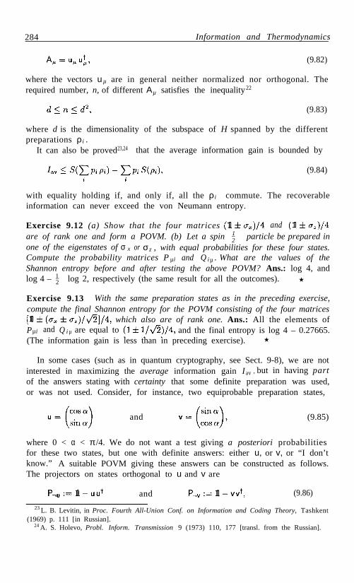
284 Information and Thermodynamics
(9.82)
where the vectors uµ are in general neither normalized nor orthogonal. Therequired number, n, of different Aµ satisfies the inequality22
(9.83)
where d is the dimensionality of the subspace of H spanned by the differentpreparations ρ i .
It can also be proved23,24 that the average information gain is bounded by
(9.84)
with equality holding if, and only if, all the ρ i commute. The recoverableinformation can never exceed the von Neumann entropy.
Exercise 9.12 (a) Show that the four matrices andare of rank one and form a POVM. (b) Let a spin 1 particle be prepared inone of the eigenstates of σ x or σCompute the probability matrices P
z , with equal probabilities for these four states.µ i and Q iµ . What are the values of the
log 4 – log 2, respectively (the same result for all the outcomes).
–2
Shannon entropy before and after testing the above POVM? Ans.: log 4, and12–
Exercise 9.13 With the same preparation states as in the preceding exercise,compute the final Shannon entropy for the POVM consisting of the four matrices
which also are of rank one. Ans.: All the elements ofPµ i and Q i µ are equal to and the final entropy is log 4 – 0.27665.(The information gain is less than in preceding exercise).
In some cases (such as in quantum cryptography, see Sect. 9-8), we are notinterested in maximizing the average information gain Iav , but in having partof the answers stating with certainty that some definite preparation was used,or was not used. Consider, for instance, two equiprobable preparation states,
and (9.85)
where 0 < α < π/4. We do not want a test giving a posteriori probabilitiesfor these two states, but one with definite answers: either u, or v, or “I don’tknow.” A suitable POVM giving these answers can be constructed as follows.The projectors on states orthogonal to u and v are
and (9.86)
23 L. B. Levitin, in Proc. Fourth All-Union Conf. on Information and Coding Theory, Tashkent(1969) p. 111 [in Russian].
24 A. S. Holevo, Probl. Inform. Transmission 9 (1973) 110, 177 [transl. from the Russian].

Neumark’s theorem 285
respectively. Let S = ⟨ u,v⟩ = sin 2α. Then the three positive operators
(9.87)
are the required POVM.
Exercise 9.14 Show that and that theprobability of an inconclusive answer is S.
After an inconclusive answer, Shannon’s entropy still has its initial value, log 2.The mean information gain with this method thus is Iav = (1 – S )log 2.
A larger gain can be achieved if we are willing to accept probabilities, ratherthan occasional certainties mixed with totally inconclusive answers. To get thislarger I av , we measure the operator whose eigenvalues are ± cos 2αThe probabilities of obtaining these eigenvalues, after preparations of u or v,are and the average information gain is
(9.88)
Exercise 9.15 Plot this result as a function of α, and show that it is alwayslarger than I av = (1 – sin 2α )log 2, which was obtained with the precedingmethod. Hint: Differentiate both expressions with respect to cos 2α .
9-6 . Neumark’s theorem
It will now be shown that there always exists a physical mechanism (that is, arealizable experimental procedure) generating any desired POVM representedby given matrices A . This result follows from Neumark’s theorem, 25,26
µ whichasserts that one can extend the Hilbert space of states H , in which the Aµ
are defined, in such a way that there exists, in the extended space K, a set oforthogonal projectors Pµ satisfying and such that Aµ is the result ofprojecting Pµ from K into H. (The actual realizability of this set of Pµ followsfrom the strong superposition principle, see page 54.)
Thanks to Davies’s theorem,22 we can restrict our attention to matrices Aµ
that are of rank one, as in Eq. (9.82). The index µ runs from 1 to N, the numberof different outcomes (note that N ≥ n if all the A µ have rank 1, the equalitysign holding only if they are orthogonal). Let us add N – n extra dimensionsto H by introducing unit vectors vs , orthogonal to each other and to all the uµ
in Eq. (9.82). The index s runs from n + 1 to N. Consider
25M. A. Neumark, Izv. Akad. Nauk SSSR, Ser. Mat. 4 (1940) 53, 277; C. R. (Doklady) Acad.Sci. URSS (N.S.) 41 (1943) 359.
26N. I. Akhiezer and I. M. Glazman, Theory of Linear Operators in Hilbert Space, Ungar,New York (1963) Vol. 2, pp. 121–126.

286 Information and Thermodynamics
(9.89)
where the c µs are complex coefficients to be determined. The vectors w µ forma complete orthonormal basis in the enlarged space K provided that
(9.90)
There are here more equations than unknown coefficients cµ s . However, the uµ
are not arbitrary: they obey the closure property Explicitly,
(9.91)
where i and j run from 1 to n (the number of dimensions of the original Hilbertspace, H ). With the same explicit notations, Eq. (9.90) is
Consider now the square matrix of order N ,
(9.92)
(9.93)
The first n columns are the u λ i , which are given, and the ( N – n ) remainingcolumns are the unknown cλs . Equation (9.92) simply states that M is a unitarymatrix. The first n columns, which satisfy the consistency requirement (9.91),can be considered as n orthonormal vectors in a N -dimensional space. There arethen infinitely many ways of constructing N–n other orthonormal vectors forthe remaining columns. We thereby obtain explicitly the N orthonormal vectorsw µ defined by Eq. (9.89). Their projections into H are the uµ of Eq. (9.82).
Exercise 9.16 Write explicitly the matrix M for the POVM in (9.87).
We now have a formal proof of Neumark’s theorem (for a finite dimensionalHilbert space) but we still have the problem of actually constructing the extradimensions spanned by the vectors v s . In some cases, this is easy: it may happenthat the set of u µ in Eq. (9.82) spans only a subspace of the states availableto our quantum system, and that the latter has enough states to accomodateall the vs (it is trivially so if we use only a finite number of Aµ in an infinitedimensional Hilbert space). However, in general, the extension from H to Knecessitates the introduction of an ancilla, 19 as shown below.

Neumark’s theorem 287
Case study: three non-orthogonal states
As a simple example, let n1 , n2 and n 3 denote three unit vectors making anglesof 120° with each other, so that Consider a spin 1
–2
particle and definethree pairs of normalized states by
and (9.94)
It is easily verified that the three positive operators
(9.95)
have sum and therefore define a POVM.Suppose that we are given the following information: The spin
1–2
particle canbe prepared in one of the three quantum states Xµ defined above, and thesethree preparations have equal a priori probabilities. If we are not told whichone of the three X µ is actually implemented, the Shannon entropy is H = log 3.Our problem is to devise a procedure giving us as much information as possible(that is, reducing H as much as possible).
Exercise 9.17 Show that in this case the Levitin-Holevo inequality (9.84)gives I av < log 2.
We shall now see that the best result which can be achieved is to reduce thevalue of H to log2, so that the actual information gain is log(3/2). This resultis obtained by ruling out one of the three allowed states, and leaving equala posteriori probabilities for the two others (see next exercise).
The actual mechanism can be described as follows. The ancilla, which also isa spin
1–2 particle, is prepared in an initial state φ 0 . Let φ ' be the state orthogonal
to φ0 . Let ψ be any arbitrary state of the original particle, and let ψ ' be theorthogonal state. Choose phases in such a way thatThen the three states19
(9.96)
are orthonormal. The fourth orthonormal state is The four projectionoperators therefore form an orthogonal resolution of the identity,and can in principle be measured in a single maximal test. Moreover, we have
(for µ = 1,2,3) and therefore, 27
(9.97)
as in Eq. (9.80). In this particular case, it can be shown 22 that the A µ inEq. (9.95) are the optimal set which maximizes Iav .
27 Here, denotes the “partial inner product” of the ancilla state φ0 with the combinedstate . The latter is defined in a larger Hilbert space, namely the tensor product of theancilla’s Hilbert space with the original H. The value of this partial inner product therefore isa vector in H .

288 Information and Thermodynamics
Exercise 9.18 Show that and that the finalentropy is Hµ = log 2 (the same entropy for all outcomes).
Preparation of the ancilla for arbitrary Aµ
This construction will now be generalized to an arbitrary set of A µ . Let φ 0
be the initial state of the ancilla, and let , be other states in theancilla’s Hilbert space, forming together with φ0 an orthonormal basis (that is,the ancilla is an N – n + 1 state system). Likewise, let e k denote a completeorthonormal basis in H. Define, as in Eq. (9.89),
(9.98)
The calculations now proceed just as in the previous case. However, thespan only a subspace of K, because K has n ( N – n + 1) dimensions. The( N – n )(n – 1) remaining orthonormal states can be taken as , wherek = 2 , . . . , n . All these states are orthogonal to φ0 and therefore do not affectthe validity of Eq. (9.97).
Exercise 9.19 Construct the vector for the POVM (9.87).28,29
Exercise 9.20 Consider four unit vectors n µ connecting the center of a tetra-hedron to its vertices, so that the angle between any two of these vectors isπ – arccos 1–
3 . Define X µ , ψµ and A µ as in Eqs. (9.94) and (9.95). Constructexplicitly the matrix M in Eq. (9.93). Assuming that the four input states ψ µ
are equally probable, show that the information gain is log(4/3).
In real life, POVMs are not necessarily implemented by the algorithm ofEq. (9.98). There is an infinity of other ways of materializing a given POVM.The importance of Neumark’s theorem lies in the proof that any arbitraryPOVM with a finite number of elements can in principle, without violating therules of quantum theory, be converted into a maximal test, by introducing anauxiliary, independently prepared quantum system (the ancilla).
Quantum state resulting from a POVM
After a repeatable maximal test, the new state of the quantum system is thepure state which corresponds to the outcome found in that test. What happensafter we execute a POVM? The result essentially depends on how that POVMis implemented. 30 For example, if we use the method which has just beendescribed and we find the result µ, the state of the combined system is givenby Eq. (9.98). The reduced density matrix of the original quantum system isobtained by taking a partial trace on the ancilla’s variables,27
28 D. Dieks, Phys. Letters A 126 (1988) 303.29 A. Peres, Phys. Letters A 128 (1988) 19.30 S L Braunstein and C. M. Caves, Found. Phys. Lett. 1 (1988) 3.

The limits of objectivity 289
(9.99)
The last sum is as may be seen by setting λ = µ inEq. (9.90). Therefore the state of the quantum system after we have found theµ -th outcome of the POVM by the above method is
(9.100)
If our quantum system was in state ρ, the probability of finding outcome µ isTr (Aµ ρ). Therefore the expected state after execution of this POVM is
(9.101)
A special case of this result is von Neumann’s projection valued measure, whereAµ = P µ . We then have Tr A µ = 1, and
Exercise 9.21 Derive the last expression in Eq. (9.102).
(9.102)
Exercise 9.22 Show that, if we again test the same POVM, the probabilityof getting result v is
(9.103)
9-7. The limits of objectivity
Your supplier of polarized particles (the beam physicist of your accelerator)claims to have produced neutrons with spin up. Can you verify this? If yourphilosophy is that of the logical positivists, a statement is meaningful only if itis possible to establish empirically whether it is true or false. Obviously, youcan take one of these neutrons and perform a Stern-Gerlach type experiment.If the answer is “down,” you have caught your beam physicist misleading you;but if the answer is “up,” this does not prove as yet that he told the truth.A neutron polarized at an angle θ from “up” has a probability cos²(θ/2) toyield the “up” result in a Stern-Gerlach experiment. An unpolarized neutron
has a 50% probability to successfully pass the test.The notions of truth and falsehood acquire new meanings in the logic of
quantum phenomena. It is in principle impossible to establish by a single testthe veracity of a statement about a quantum preparation. You can increase theconfidence level by testing more than one neutron, but this, in turn, dependson your willingness to rely on the uniformity of the neutrons preparations. This

290 Information and Thermodynamics
issue itself is amenable to a test, but only if other suitable assumptions are made.In general, the residual entropy (i.e., the uncertainty) left after a quantum testdepends on the amount and type of information that was available before thetest. This is also true in classical information theory (since Ia v depends on thea priori probabilities pi ) but the effect is more striking for quantum informationwhich can be supplied in subtler ways.
State verification
Let us start with an elementary example. You are told that a spin 1–2
particlewas prepared in an eigenstate of σz , with equal probabilities for both states.The Shannon entropy is log 2, and this also is the von Neumann entropy, since
A Stern-Gerlach test along the z direction can then determine theinitial state with certainty. The information gain is log 2.
Now, imagine that there are two observers, who give contradictory reports onthe spin preparation procedure. One of them tells you that it is an eigenstate ofσx (with equal probabilities for both signs) and the other one asserts that it isan eigenstate of σ y (also with equal probabilities for both signs). If you equallytrust (or distrust) your two observers, the Shannon entropy is log 4. You decideto perform a Stern-Gerlach test.
Exercise 9.23 What is the information gain if that test is performed alongthe x direction? Along a direction bisecting the angle between the x and yaxes? Ans.: Iav = 0.34657 and 0.27665, respectively.
The above exercise shows that different testing methods may yield differentamounts of information, which is not unexpected. However, no testing what-soever can determine which one of the two observers told the truth. This isimpossible even if you are given an unlimited number of particles to test. Thisimpossibility is fundamental (it follows from Postulate K, page 76). Indeed, ifit were not so, instantaneous communication between distant observers wouldbe possible, by using correlated pairs of particles originating from a commonsource halfway between them, as was shown in Chapter 6.
Continuous variables: a case study
Suppose that the only information prior to a test of σz is that the initial statewas pure. It satisfied with equal probabilities for all directions ofthe unit vector n. How well can we determine n?
Let us parametrize n by the polar angle θ and the azimuthal angle φ aroundthe z -axis. The outcomes ±1 of the test for σ z have probabilities
(9.104)
This test therefore gives no information about φ (as is obvious, because of theaxial symmetry).

The limits of objectivity 291
With an isotropic distribution of the spin direction n, the a priori probabilitypθ for the polar angle θ, irrespective of the value of φ, is given by p θ d θ =sin Let us introduce a new variable, u = cos θ,a n ddivide the domain of u into a large number N of equal intervals of size du = 2/N .The a priori probability for any one of these small intervals is
(9.105)
The initial Shannon entropy is
(9.106)
In the limit N → ∞, the value of H 0 becomes infinite, but this is harmless,because H0 is an irrelevant additive constant, as we shall see. (A similar infinityalso occurs in the definition of entropy in classical statistical mechanics.31)
Exercise 9.24 What is the density matrix corresponding to a given value ofu = cos θ, in the representation where σ z is diagonal?
The a priori probabilities for the outcomes ±1 in a test for σz are
The a posteriori probability for u therefore is, by Bayes’s theorem,
and the final Shannon entropy, after observation of an outcome ±1, i s
The average information gain thus is
(9.108)
(9.107)
(9.109)
(9.110)
As expected, the information gain is smaller than in the previous examples,where there were only a few distinct possibilities for the value of u = cos θ.
Exercise 9.25 Generalize the above discussion to the case where the a prioriprobability for the direction of n is not isotropic.
31 F. Reif , Fundamentals of Statistical and Thermal Physics, McGraw-Hill, New York (1965)p. 245.

292 Information and Thermodynamics
statistical problem.
What happens if we know nothing at all about the initial preparation?Strange as it may be, there is no possibility of “knowing nothing” in the presentcontext. The only valid questions are those of the following type: Given thea priori probabilities of various preparations, estimate their a posteriori prob-abilities, after the result of the test is known. Within this logical framework,a statement that the initial state is a random mixture, ρ ~ , leaves no roomfor a priori probabilities. It is a complete specification of the preparation: theShannon entropy is zero and no further information is to be sought. It is onlywhen several distinct alternatives are considered that we have a meaningful
Homogeneous assemblies
Consider a large number n of independent quantum systems of a known type.The supplier asserts that the states of all these systems have been prepared inthe same way. If he does not disclose what that state is, it is easy to determine itempirically: the elements of ρ (a density matrix of order N) can be obtained bymeasuring the mean values of N 2 – 1 suitably chosen operators.32 (The exampleof a 2 × 2 density matrix was discussed in detail, page 76.) The problem is toverify that these n systems have indeed been prepared in the same way—forexample, that the source of particles which produces them is well stabilized.
Recall that quantum theory describes a set of n independently prepared sub-systems by a density matrix . This is a direct product,where each one of the ρj matrices is of order N. The matrix R is of order N n
and treats the assembly as a single composite system. If all the subsystemsare prepared in the same way, the ρj matrices are identical. They depend onN 2 – 1 parameters which can be measured experimentally.32 We shall now seethat if n N 2 , it is possible to verify the uniformity of the preparations.
We divide the n subsystems into v sets, in any suitable systematic way—notin a random way-so as to avoid erasing any suspected systematic deviationsfrom homogeneity in the preparation procedure. For example, yesterday’s sam-ples are not mixed with those of the preceding day, if we suspect that the sourceis not stable. A convenient way of distributing the n samples among v sets isto take v ~ N so that n v N 2 . We then use N 2 –1 of these sets toobtain estimates of the elements of ρ, and we repeat this process many times,to verify that the results of different samples are consistent. If no inconsistencyis found beyond the normally expected statistical fluctuations, we are satisfiedthat the n subsystems have been prepared in the same way, and we have alsomeasured the corresponding one-particle density matrix ρ.
Here, it should be noted that we have asked only a very small subset ofall the possible questions: while only N 2 – 1 different questions are needed fordetermining ρ, a maximal test could have had N n different outcomes (this is thedimensionality of R). We shall again see in Chapter 12 that the transition from
32 W. Band and J. L . Park, Found. Phys. 1 (1971) 339; Am. J. Phys. 47 (1979) 188.

Quantum cryptography and teleportation 293
9-8.
the quantal to the classical description of a physical system requires discardingnearly all the microscopic information pertaining to that system.
Quantum cryptography and teleportation
Cryptography is the art of transmitting information in such a way that it cannotbe understood by an opponent who might intercept it. The original information,called plaintext, consists of words or expressions taken from a finite vocabularyand assembled according to definite syntactical rules. Encryption is an invertibledeterministic mapping, yielding a ciphertext which conforms to none of theserules and appears random and meaningless, so that it can be safely transmittedover a public communication channel.
A demonstrably safe encryption method is the Vernam cipher. The plaintextis written as sequence of bits (0 and 1). Another random sequence, called akey, is added to it, bit by bit, modulo 2. This addition is equivalent to theBoolean operation XOR (exclusive OR). The resulting ciphertext can then bedecrypted by XORing it with the same key. It is essential to use a key as longas the message, and to never use it again. 33
The problem we are going to address is how to distribute a cryptographickey (a secret sequence of bits) to several observers who initially share no secretinformation, by using an insecure communication channel subject to inspectionby a hostile eavesdropper. If only classical means are used, this is an impossibletask. Quantum phenomena, on the other hand, provide various solutions. Thereason for this difference is that information stored in classical form, such asprinted text, can be examined objectively without altering it in any detectableway, let alone destroying it, while it is impossible to do that with quantizedinformation encoded in unknown non-orthogonal states, for instance in thepolarizations of photons. It is the elusiveness of quantum information whichmakes it ideal for transmitting secrets.
EPR key distribution
Consider a source of correlated photon pairs, as in the Aspect experiment (seeFig. 6.8, p. 166). Two distant observers receive these photons and test theirpolarizations along directions α or β, which make a 45° angle with each other.Here, contrary to the original Aspect experiment, the same pair of directionsis used by both observers. The choice between α and β is randomly madefor each photon, by each observer, who keeps a record of the results of all hispolarization tests. After they have analyzed a sufficient number of photon pairs,
33 If two messages are XORed with the same key, the XOR of their ciphertexts is identicalto the XOR of the plaintexts. The result is equivalent to the use of one of the messages as anon-random key for encrypting the other message. If only a finite vocabulary is used, it thenis an easy cryptographic problem to decipher both messages.
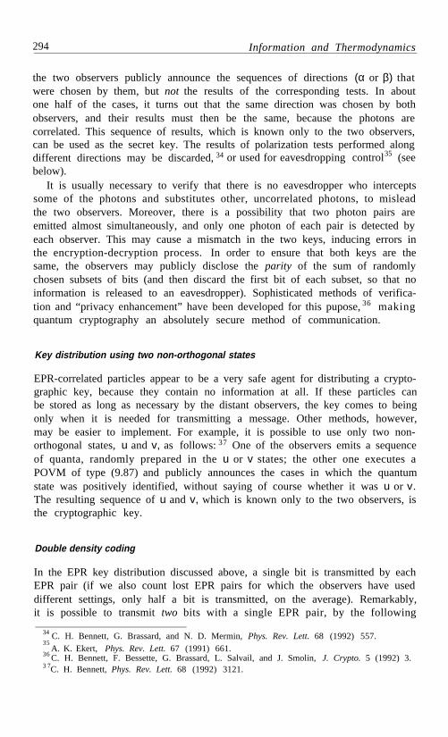
294 Information and Thermodynamics
the two observers publicly announce the sequences of directions (α or β) thatwere chosen by them, but not the results of the corresponding tests. In aboutone half of the cases, it turns out that the same direction was chosen by bothobservers, and their results must then be the same, because the photons arecorrelated. This sequence of results, which is known only to the two observers,can be used as the secret key. The results of polarization tests performed alongdifferent directions may be discarded, 34 or used for eavesdropping control35 (seebelow).
It is usually necessary to verify that there is no eavesdropper who interceptssome of the photons and substitutes other, uncorrelated photons, to misleadthe two observers. Moreover, there is a possibility that two photon pairs areemitted almost simultaneously, and only one photon of each pair is detected byeach observer. This may cause a mismatch in the two keys, inducing errors inthe encryption-decryption process. In order to ensure that both keys are thesame, the observers may publicly disclose the parity of the sum of randomlychosen subsets of bits (and then discard the first bit of each subset, so that noinformation is released to an eavesdropper). Sophisticated methods of verifica-tion and “privacy enhancement” have been developed for this pupose, 36 makingquantum cryptography an absolutely secure method of communication.
Key distribution using two non-orthogonal states
EPR-correlated particles appear to be a very safe agent for distributing a crypto-graphic key, because they contain no information at all. If these particles canbe stored as long as necessary by the distant observers, the key comes to beingonly when it is needed for transmitting a message. Other methods, however,may be easier to implement. For example, it is possible to use only two non-orthogonal states, u and v, as follows: 37 One of the observers emits a sequenceof quanta, randomly prepared in the u or v states; the other one executes aPOVM of type (9.87) and publicly announces the cases in which the quantumstate was positively identified, without saying of course whether it was u or v.The resulting sequence of u and v, which is known only to the two observers, isthe cryptographic key.
Double density coding
In the EPR key distribution discussed above, a single bit is transmitted by eachEPR pair (if we also count lost EPR pairs for which the observers have useddifferent settings, only half a bit is transmitted, on the average). Remarkably,it is possible to transmit two bits with a single EPR pair, by the following
34 C. H. Bennett, G. Brassard, and N. D. Mermin, Phys. Rev. Lett. 68 (1992) 557.35
A. K. Ekert, Phys. Rev. Lett. 67 (1991) 661.36 C. H. Bennett, F. Bessette, G. Brassard, L. Salvail, and J. Smolin, J. Crypto. 5 (1992) 3.3 7C. H. Bennett, Phys. Rev. Lett. 68 (1992) 3121.

Quantum cryptography and teleportation 295
procedure: 38 Consider an EPR pair distributed to two distant observers. Tosimplify the discourse, I shall use notations appropriate to spin 1 particles. The2
pair is in a singlet state, where and .To encode a message, the emitter subjects his particle to a unitary operation,
(9.111)
and sends it to the other observer. The latter thus possesses a correlated pair,in one of the states (up to an irrelevant phase)
or (9.112)
These four states are orthogonal and a maximal test can distinguish them un-ambiguously, thereby revealing which unitary operation was performed. On theother hand, an eavesdropper who would intercept the information carrier wouldfind it in a useless random mixture, (that is, if the same procedure,with the same unitary operation, is repeated many times).
Quantum teleportation
The inverse process is even more remarkable. It is the “teleportation” of anunknown quantum state by means of an EPR pair and two bits of classicalinformation. 39 The first step of this process is the distribution of the EPR pair,in the standard singlet state, to the distant observers, A and B. Suppose thatA holds, besides particle 1, another spin 1 particle, labelled 0, in an unknown2state φ that has to be transmitted to B (the particle itself is not sent, onlyinformation specifying its unknown state). This can be done as follows.
Particles 0 and 1, which are initially uncorrelated, are subjected by A to amaximal quantum test with eigenstates
and (9.113)
These are analogous to the states in (9.112). The four outcomes of this test haveequal probabilities, regardless of the unknown state φ (see exercise below). Theresult of the test—two apparently random bits of information—is communicatedto B over a public channel. According to this result, B performs on particle 2a suitable unitary operation from the set (9.111). The state of particle 2 thenbecomes φ, identical to the state of particle 0 before the latter was tested by A.That state now is inaccessible to A, and is still unknown to B.
The experimental meaning of the above statements is the following: there isa 25% probability that A finds state Ψ – ; then, if B measures any projectionoperator P, the probability of getting the result 1 is ⟨φ, Pφ⟩. Likewise, if Afinds state Ψ + , and B measures P, the probability of getting the result 1 is⟨σ z φ, Pσz φ⟩; and so on. The detailed proof is proposed as the following exercise:
38 C. H. Bennett and S. J. Wiesner, Phys. Rev. Lett. 69 (1992) 2881. 39 C. H. Bennett, G. Brassard, C. Crépeau, R. Jozsa, A. Peres, and W. K. Wootters, Phys.
Rev. Lett. 70 (1993) 1895.
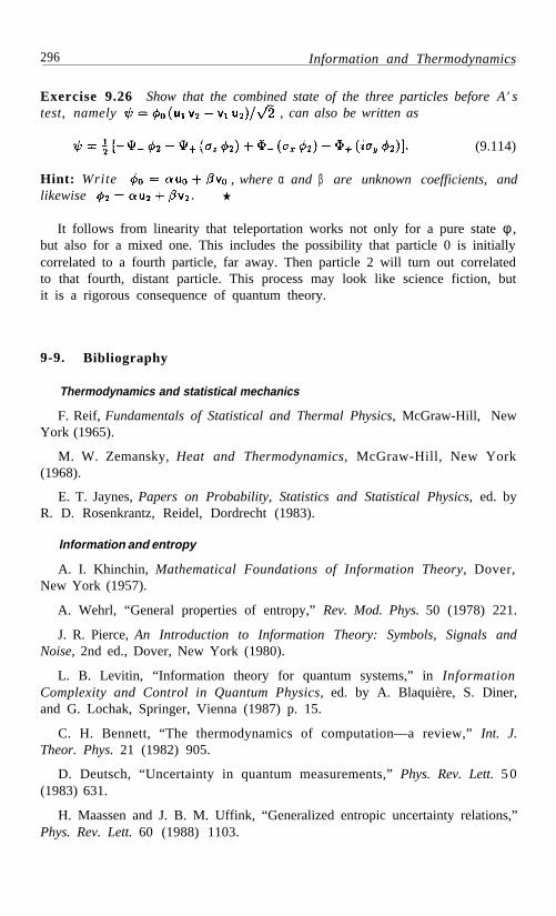
296 Information and Thermodynamics
Exercise 9.26 Show that the combined state of the three particles before A' stest, namely , can also be written as
(9.114)
Hint: Write , where α and β are unknown coefficients, andlikewise
It follows from linearity that teleportation works not only for a pure state φ ,but also for a mixed one. This includes the possibility that particle 0 is initiallycorrelated to a fourth particle, far away. Then particle 2 will turn out correlatedto that fourth, distant particle. This process may look like science fiction, butit is a rigorous consequence of quantum theory.
9-9. Bibliography
Thermodynamics and statistical mechanics
F. Reif, Fundamentals of Statistical and Thermal Physics, McGraw-Hill, NewYork (1965).
M. W. Zemansky, Heat and Thermodynamics, McGraw-Hill, New York(1968).
E. T. Jaynes, Papers on Probability, Statistics and Statistical Physics, ed. byR. D. Rosenkrantz, Reidel, Dordrecht (1983).
lnformation and entropy
A. I. Khinchin, Mathematical Foundations of Information Theory, Dover,New York (1957).
A. Wehrl, “General properties of entropy,” Rev. Mod. Phys. 50 (1978) 221.
J. R. Pierce, An Introduction to Information Theory: Symbols, Signals andNoise, 2nd ed., Dover, New York (1980).
L. B. Levitin, “Information theory for quantum systems,” in InformationComplexity and Control in Quantum Physics, ed. by A. Blaquière, S. Diner,and G. Lochak, Springer, Vienna (1987) p. 15.
C. H. Bennett, “The thermodynamics of computation—a review,” Int. J.Theor. Phys. 21 (1982) 905.
D. Deutsch, “Uncertainty in quantum measurements,” Phys. Rev. Lett. 5 0(1983) 631.
H. Maassen and J. B. M. Uffink, “Generalized entropic uncertainty relations,”Phys. Rev. Lett. 60 (1988) 1103.

Bibliography 297
Maxwell’s demon
H. S. Leff and A. F. Rex, eds. Maxwell’s Demon: Entropy, Information,Computing, Adam Hilger, Bristol (1990).
Maxwell introduced his legendary demon as a challenge to second law of thermo-dynamics. The problem is whether a microscopic intelligent being can cause a decreaseof entropy in a thermodynamic system. The various answers that have been giveninvolve statistical physics, quantum theory, information theory, and computer science.A didactic overview of the problem precedes this collection of reprints which includes,among others, an English translation of Szilard’s historic article “On the decrease ofentropy in a thermodynamic system by the intervention of intelligent beings,” Z. Phys.53 (1929) 840. Important recent contributions are:
C. H. Bennett, “Demons, engines and the second law,” Sci. Am. 257 (Nov.1987) 88.
C. M. Caves, “Quantitative limits on the ability of a Maxwell demon toextract work from heat,” Phys. Rev. Lett. 64 (1990) 2111.
Some comments on the last article, by C. M. Caves, W. G. Unruh, and W. H. Zurek,appear in Phys. Rev. Lett. 65 (1990) 1387.
Nonlocal effects
S. L. Braunstein and C. M. Caves, “Information-theoretic Bell inequalities,”Phys. Rev. Lett. 61 (1988) 662.
B. W. Schumacher, “Information and quantum nonseparability,” Phys. Rev.A 44 (1991) 7047.
A. Peres and W. K. Wootters, “Optimal detection of quantum information,”Phys. Rev. Lett. 66 (1991) 1119.
This paper discusses the optimal stategy for determining the common state of twoquantum systems, identically prepared in different locations. A single combined test,performed on both systems together, is more efficient than various combinations ofPOVMs for each system separately. However, the problem of finding the best separate-particle strategy is left unsolved, and it is proposed as a challenge to quantum theorists.
Quantum communication, cryptography, and computation
C. M. Caves and P. D. Drummond, “Quantum limits on bosonic communi-cation rates,” Rev. Mod. Phys. 66 (1994) 481.
R. Jozsa and B. Schumacher, “A new proof of the quantum noiseless codingtheorem,” J. Mod. Optics 41 (1994) 2343.
A. K. Ekert, B. Huttner, G. M. Palma, and A. Peres, “Eavesdropping onquantum-cryptographical systems,” Phys. Rev. A 50 (1994) 1047.
A. Barenco, D. Deutsch, A. Ekert, and R. Jozsa, “Conditional quantumdynamics and logic gates,” Phys. Rev. Lett. 74 (1995) 4083.

Chapter 10
Semiclassical Methods
10 -1. The correspondence principle
The historical development of quantum mechanics left it with a heavy legacy ofclassical concepts. Foremost among them is the correspondence principle, whichasserts that there are, under suitable conditions, analogies between classical andquantum dynamics. Even today, this principle is often used as an intuitive guidefor finding quantum properties similar to known classical laws. These analogiesare surprising, because of the radical differences in the mathematical formalismsunderlying the two theories: quantum mechanics uses a separable Hilbert spacewith a unitary inner product, while classical mechanics wants a continuousphase space with a symplectic structure.¹ Yet, in spite of this fundamentaldifference, there may be in some situations an approximate correspondencebetween classical and quantum concepts. The analogy is admittedly vague.Some of its virtues and limitations are pointed out below. In particular, it willbe shown how the correspondence principle must ultimately break down in anynontrivial problem.
Classical operators
Formally, we may imagine a sequence of quantum theories having differentvalues of and examine under which conditions the limit exists andcoincides with classical mechanics. In general, for arbitrary dynamical vari-ables, this limit does not exist and quantum theory does not reduce to classicalmechanics. However, in that sequence of quantum theories, there is a privilegedclass of operators, which can be expressed in terms of the canonical q and p,without explicit mention of . These have been called reasonable or classicaloperators. 2,3 For instance, the momentum operator introduced in Sect. 8-4 isreasonable. Likewise is reasonable, but cos is not. By
¹H. Goldstein, Classical Mechanics, Addison-Wesley, Reading (1980) pp. 391–407.²L. G. Yaffe, Rev. Mod. Phys. 54 (1982) 407.³K. B. Kay, J. Chem. Phys. 79 (1983) 3026.
298

The correspondence principle 299
“neighboring” outcomes of quantum tests. In pure quantum theory, this is a
restricting our attention to these special operators, it becomes possible to findsimilarities between classical properties and corresponding quantum properties,in an appropriate limit loosely called .
Such a limiting process was used in Sect. 6-6, when we lumped together
meaningless phrase: any two different outcomes of a quantum test correspondto orthogonal states, and are as close or distant as any two other differentoutcomes. However, a meaning can be attributed to “neighboring” outcomesin a semiclassical context, where the outcomes that are lumped together arethose which correspond to neighboring eigenvalues of reasonable operators. Theargument presented in Sect. 6-6 was that, if our macroscopic apparatuses areable to measure only operators of that type, it is impossible to observe thestrong correlations predicted by quantum mechanics for the results of tests per-formed at distant locations. The readings of our instruments have only weakerclassical correlations, which do not violate Bell’s inequality. It is only whenour instruments are so keen that they can detect genuine quantum features,such as isolated eigenvalues, that local realism breaks down (together with thecorrespondence principle itself).
Canonical and unitary transformations
A formal analogy, emphasized by Dirac,4 is the one between canonical transfor-mations in classical mechanics and unitary transformations in quantum theory.(The reader who is not familiar with canonical transformations should consultthe bibliography at the end of Chapter 1.) Obviously, there cannot be any strictcorrespondence between these two concepts, because unitary transformationspreserve eigenvalues (which are the observable values of quantum dynamicalvariables) while canonical transformations can relate variables having differentdomains of definition and even different dimensions. An example of failure ofthis correspondence for “unreasonable” operators will be given later. First, letus see some cases where it works.
A question which often arises in practice is the following: given a classicalphysical system, how do we define the analogous quantum mechanical system?This surely is an ill defined question, to which I can only propose the followingill defined answer: The law of motion of reasonable quantum operators (in theHeisenberg picture) should resemble the classical law of motion. This criterionis admittedly vague, because any resemblance between these laws is in the eyeof the beholder. I shall now illustrate this issue by simple examples, using asdynamical variables the three components of angular momentum.
First, assume that the quantum law of motion is a rotation by an angle βaround the y-axis. That rotation is represented by the unitary operator
(10.1)
4 P. A. M. Dirac, The Principles of Quantum Mechanics, Oxford Univ. Press (1947), p. 106.

300 Semiclassical Methods
Obviously, this operator has no limit for , if the classical parameter βand the classical operator Jy are kept fixed while changes. The operator Uhas an essential singularity for . We do not obtain classical mechanics asa limiting case of quantum mechanics.
The relationship between U , in Eq. (10.1), and a classical rotation aroundthe y-axis has a formal nature: We note that J itself is invariant under they
unitary transformation generated by U . For the other components, we have
(10.2)
and some algebraic manipulations (best done in the representation where Jy isdiagonal) give
(10.3)
Written in this form, the quantum law of motion looks identical to a classicalrotation. In particular, it does not involve explicitly.
As a second example, consider a linear twist around the z-axis, by an angleproportional to J z / J :
(10.4)
This is a canonical tranformation of the variables Jx , Jy and Jz, as can be seenfrom the fact that the J'n have the same Poisson brackets as the Jn.
In quantum theory, we may still assume that the total angular momentumhas a sharp value, . For any given J, the twist operator is
(10.5)
This unitary operator leaves Jz invariant, and the law of motion of the othercomponents is
(10.6)
Note that U has no limit for . With some algebraic manipulations (bestdone in the representation where Jz is diagonal), Eq. (10.6) can be written as
(10.7)
where both exponents now have the same sign, not opposite signs as in (10.6).
Exercise 10.1 Verify that the transformation (10.4) is canonical.
Exercise 10.2 Verify Eq. (10.7).

The correspondence principle
Again, seems to have disappeared. It still is here implicitly, of course, becauseof its presence in the commutation relations of the components of J. However,if we pretend that the variables in Eq. (10.7) are classical, that equation can bewritten as
(10.8)
which looks exactly like the twist transformation in Eq. (10.4).
Unreasonable operators
The correspondence principle completely fails when we consider canonical trans-formations between classical variables whose quantum analogs have differentspectra, and cannot therefore be related by unitary transformations. Even themost fundamental notion of classical mechanics, that of number of degrees offreedom, has no quantum counterpart.
Exercise 10.3 What is the canonical transformation from Cartesian to spher-ical coordinates? Write explicitly the canonical momenta pθ and pφ in termsof the Cartesian momenta p. What is the canonical transformation from thevariables θ, φ, pθ, p φ , to a new set of variables, among which
and
(10.10)
301
(10.9)
(whose Poisson bracket vanishes) are the two new canonical momenta? Whatare the canonical coordinates conjugate to J z and J 2 ? If these dynamicalvariables are converted into operators, what are their domains of definition?
Ans.: The generating function of the second canonical transformation is
and the corresponding coordinates are
(10.11)
and
(10.12)
As a sequel to this exercise, let us perform one more canonical transformation,and define new momenta and their conjugate coordinatesQ ±. What are the quantum analogs of these variables? These are not reasonableoperators, of course, since their definition involves explicitly. Nonetheless,they have a perfectly well defined domain in Hilbert space. The eigenvalues ofP± are all the positive integers, as seen in the following table:

302 Semiclassical Methods
The operators P+ and P– are nondegenerate, and they are functions of eachother. Consider the representation where both are diagonal. If there were acorrespondence between Poisson brackets and commutators, we would expectP+ to commute with Q – , and therefore Q – would be diagonal too. This wouldthen contradict the requirement that Q – is conjugate to P– . Not surprisingly,the correspondence principle fails for these nonclassical operators.
10-2. Motion and distortion of wave packets
Until now, we considered algebraic properties of operators, irrespective of thechoice of specific quantum states. There also are analogies of a different type,holding for localized states such as wave packets. For simplicity, consider asystem with a single degree of freedom, and a HamiltonianThe Heisenberg equations of motion are
and (10.13)
Let q = and p = denote the mean values of the operators q and p. We then have, from (10.13),
and (10.14)
Therefore, if the potential V changes slowly over the size of a wave packet,so that the wave packet moves approximately like aclassical particle. This is Ehrenfest’s theorem.5
Let us evaluate deviations from this semiclassical approximation. We have,by a Taylor expansion,
(10.15)
whence
(10.16)
When we take the expectation value of the last equation, we havea n d which is the dispersion of q (the width of the wavepacket). We obtain, neglecting and higher terms,
5 P. Ehrenfest, Z. Phys. 45 (1927) 455.

Motion and distortion of wave packets 303
(10.19)
(10.17)
Because of the last term, the centroid of a wave packet does not move alonga classical orbit, and there is a gradual spreading and distortion of the wavepacket. 6 (Note, however, that these are not quantum phenomena: similar effectsalso occur for classical Liouville densities.)
Poincaré invariants
This difference between the motion of localized wave packets and that of clas-sical point particles has important consequences. In particular, it precludesthe existence of quantum analogs for the classical Poincaré invariants.7,8 Thesimplest of these invariants is the volume of a 2N -dimensional domain in phasespace. As the points which form the boundary of this domain move according toHamilton’s equations, the enclosed volume remains constant—this is Liouville’stheorem. Any compact domain, obeying the Liouville equation of motion, iscontinuously distorted and tends to project increasingly long and thin filaments.As time passes, new, finer filaments emerge, whose volume is less than . Thequantum density ρ (or the Wigner function, that will be discussed in Sect. 10-4)cannot reproduce these minute details and smoothes them away.9 We thereforeexpect the quantum dynamical evolution to be qualitatively milder than theclassical one.
Let us examine the simple case of a single degree of freedom. There is only onePoincaré invariant: the area of a domain in phase space. The evolution of thearea of an infinitesimal triangle can be investigated by comparing three slightlydifferent motions of a given particle. In classical mechanics, these would bethree neighboring orbits in phase space. In quantum mechanics, we shall havethree neighboring wave packets, labelled and . For the wave packet
, let us define mean values q', p' and ∆ 'q, as before. We then have, fromEqs. (10.14) and (10.17),
(10.18)
and
6 M. Andrews, J. Phys. A 14 (1981) 1123.7 H. Goldstein, Classical Mechanics, 1st ed., Addison-Wesley, Reading (1950) pp. 247–250.
Unfortunately, this material was deleted from the second edition of this book.8 M. Born, The mechanics of the atom, Bell, London (1927) [reprinted by Ungar, New York
(1960)] p. 36.9 H. J. Korsch and M. V. Berry, Physica D 3 (1981) 627.

304 Semiclassical Methods
Indeed, introducing the third neighboring wave packet, with equationsof motion similar to (10.18) and (10.19), we obtain the rate of change of theinfinitesimal triangle area:10
It is the last term in this equation which precludes the existence of a quantumanalog of the area preserving theorem.
(10.20)
This expression does not vanish in general, unless It can beneglected only if the size of the wave packets is much smaller than the distancebetween the vertices of the (infinitesimal) triangle. Such an approximation maybe valid for planets and other macroscopic bodies, but not for generic quantumsystems such as atoms or molecules.
Case study: Rydberg states
If the evolution of a localized quantum wave packet cannot besimulated by that of a classical Liouville density (which represents an ensembleof particles moving on neighboring orbits in phase space) for more than a finitelapse of time, whose duration depends on the type of potential and on thelocation of the wave packet in phase space.10 The following example displayssome bizarre features of quantum dynamics, with no classical analog.
Consider the motion of a planet around the Sun, with V = –G M m/r, o rthat of an electron in a Coulomb potential, For simplicity, take acircular orbit. A classical calculation gives J = rp a n d Wethus have
and (10.21)
whence
(10.22)
In these equations, p is the tangential component of the momentum p. T h eclassical angular velocity along the orbit is
(10.23)
For neighboring circular orbits, whose energies differ by δE, we have
(10.24)
10 N. Moiseyev and A. Peres, J. Chem. Phys. 79 (1983) 5945.

Motion and distortion of wave packets 305
Inner orbits have a higher angular velocity. Consequently, the Liouville densityin phase space is sheared, as it moves along concentric orbits. If it initially isa small blob, it will gradually spread over a circular arc, until the head of thepack catches up with its tail. This will occur after a time
(10.25)
Any remaining analogy between classical motion and quantum motion mustthen break down, because the quantum wave packet will interfere with itself ina way that the classical Liouville density cannot mimic.
Let us return to quantum mechanics. Instead of (10.22) we have
(10.26)
where is an integer. Hydrogen atoms with n >> 1 (for which semi-classical approximations may sometimes be valid) are called Rydberg atoms.Consecutive energy levels are separated by as expected fromthe correspondence principle: a classical charge in circular motion radiates withthe rotational frequency ω. Each emitted photon has an energy and thishas to be the energy difference between the quantized levels.
Let a hydrogen atom be prepared in such a way that the positive-energypart of its spectrum is negligible (that is, ionized atoms are removed by thepreparation procedure). The Schrödinger wave function can be expanded intoeigenfunctions of H:
(10.27)
where Since this sum converges, a finitenumber of cn can make arbitrarily close to 1, and are therefore sufficientto represent ψ with arbitrary accuracy. As a consequence, any ψ is arbitrarilyclose to a periodic function of time. Indeed, all the exponents in (10.27) havethe form where Let L be the leastcommon multiple of all the n for which we do not neglect cn . Obviously, ψ hasa period This recurrence has no classical analog (the celebrated Poincarérecurrences occur for individual orbits, not for continuous Liouville densities).
Exercise 10.4 Show that if a minimum uncertainty wave packet is placed ona circular orbit, with its central parameters satisfying Eq. (10.21), the numberof energy levels appreciably involved is of the order of
The required time for an exact recurrence, is enormous if many levelsare appreciably excited. However, nearly exact recurrences occur considerablyearlier. The probability of finding a recurrence is given by the overlap of ψ(t )with the initial state ψ (0), namely
(10.28)

306 Semiclassical Methods
where If the initial wave packet is well localized, its energy dis-persion is small and the coefficients w n are large only in a narrowdomain of n. Let N be an integer anywhere in the middle of that domain, andlet v = n – N. We can expand
(10.29)
If we keep only the first two terms of this series, the exponents in Eq. (10.28)a r e Apart from a common phase all theseexponents are integral multiples of 2πi whenever
(10.30)
where is the classical period of revolution for energy EN . This is ofcourse the expected result: for short times, the quantum wave packet moves asa classical particle. For longer times, higher terms in (10.29) destroy the phasecoherence and the wave packet spreads over the entire orbit.
Yet, it eventually reassembles: the exponent in Eq. (10.28) is, apart from anirrelevant additive constant,
(10.31)
When the second term in this series yields an integral multipleof 2πi, and the wave packet reappears at its original position. Actually, thisrecurrence already occurs after classical periods (where N, whichwas only loosely defined above, has to be adjusted so as to be a multiple of 3).Indeed, let The first two terms in (10.31) give
We can always adjust N so that N /3 is an integer. Also, V(V – 1)/2 always isan integer. Therefore, apart from terms of order N –1, the exponent in (10.31)is a multiple of 2πi. The factor N /3 (without –1 ) can also be obtained from2semiclassical arguments.11 This recurrence has been experimentally observed.12
As time passes, the third term in the series in (10.31) gradually destroysthese periodic recurrences, but new ones appear at integral multiples ofThe same argument shows that the first such reappearance actually occursat where N must again be adjusted to make it even,if necessary. These recurrences are then destroyed by the following term in(10.31), and reappear at integral multiples of and so on. Thisis illustrated in Fig. 10.1 for the case N = 1000, with 21 energy levels havinga binomial distribution of weights: Withthis value of N, the third recurrence level occurs at t = 30.4s, an exceedinglylong time by atomic standards.
11 M. Nauenberg, Comments Atom. Mol. Phys. 25 (1990) 151; J. Phys. B 23 (1990) L385.12J. A. Yeazell, M. Mallalieu, and C. R. Stroud, Jr., Phys. Rev. Lett. 64 (1990) 2007.

Classical action 307
Fig. 10.1. Recurrences of a wave packet consisting of Rydberg states withn = 990 to 1010. The value of (vertical axis) is plotted versustime. In each graph, the time (horizontal axis) extends over two classicalperiods. The central time is, from top to bottom: Tc l (one classical period),100 Tc l (a random number), 333.5 Tc l (first order recurrence), 250 000.5 Tc l
(second order recurrence), and (2 × 10⁸ + 0.5) Tc l (third order recurrence).
10-3. Classical action
A short time after the publication of Schrödinger’s historic papers, Madelung13
proposed a hydrodynamical model for Schrödinger’s equation. Letwhere R and S are real, and let ρ = R ². [In modern parlance, ρ (r) is thediagonal part of the density matrix ρ(r',r" ).] Then, the Schrödinger equationfor a particle of mass m in a potential V (r) is equivalent to the real equations:
13E. Madelung Z. Phys. 40 (1926) 322.
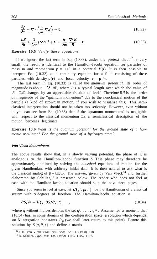
308 Semiclassical Methods
(10.32)
(10.33)
Exercise 10.5 Verify these equations.
If we ignore the last term in Eq. (10.33), under the pretext that is verysmall, the result is identical to the Hamilton-Jacobi equation for particles ofmass m and momentum p = ∇ S, in a potential V (r). It is then possible tointerpret Eq. (10.32) as a continuity equation for a fluid consisting of theseparticles, with density ρ (r) and local velocity v = p /m.
The last term in Eq. (10.33) is called the quantum potential. Its order ofmagnitude is about /ml², where l is a typical length over which the value ofR = ψ changes by an appreciable fraction of itself. Therefore /l is the orderof magnitude of the “quantum momentum” due to the nonclassical motion of theparticle (a kind of Brownian motion, if you wish to visualize this). This semi-classical interpretation should not be taken too seriously. However, even withoutit, you can see from Eq. (10.33) that if the “quantum momentum” is negligiblewith respect to the classical momentum ∇ S, a semiclassical description of themotion becomes legitimate.
Exercise 10.6 What is the quantum potential for the ground state of a har-monic oscillator? For the ground state of a hydrogen atom?
Van Vleck determinant
The above results show that, in a slowly varying potential, the phase of ψ isanalogous to the Hamilton-Jacobi function S. This phase may therefore beapproximately obtained by solving the classical equations of motion for thegiven Hamiltonian, with arbitrary initial data. It is then natural to ask what isthe classical analog of ρ = ψ ². The answer, given by Van Vleck14 and furtherelaborated by Schiller,15 is presented below. The reader who does not feel atease with the Hamilton-Jacobi equation should skip the next three pages.
Since you seem to feel at ease, let be the Hamiltonian of a classicalsystem with N degrees of freedom. The Hamilton-Jacobi equation is
(10.34)
where q without indices denotes the set q¹, . . . , q N . Assume for a moment that(10.34) has, in some domain of the configuration space, a solution which dependson N integration constants P µ (we shall later return to this point). Denote thissolution by S (q ,P , t ) and define a matrix
14J. H. Van Vleck, Proc. Nat. Acad. Sc. 14 (1928) 178.15 R. Schiller, Phys. Rev. 125 (1962) 1100, 1109, 1116.

Classical action 309
(10.35)
This matrix too is a function of q and P. The inverse matrix is defined by
(10.36)
Other functions of q and P are the momentum and the velocity:
(10.37)
Note thatIt will now be shown that the Van Vleck determinant, D = Det , satisfies
an equation of continuity in the N dimensional configuration space. We have
(10.38)
because is the coefficient of in an expansion of the determinant D(recall the rule for computing the inverse of a matrix). To obtain wedifferentiate twice the Hamilton-Jacobi equation (10.34), and obtain
(10.39)
Therefore
(10.40)
Using Eq. (10.36) and
(10.41)
which follows from the definition of , we obtain
(10.42)
This result looks like an equation of continuity for a fluid of density D andvelocity vi , in the N -dimensional configuration space. We are therefore led tointerpret the function D ( q,P,t ) as a probability density, which still needs a nor-malization factor To see this more precisely, recall that S ( q, P, t)is the generating function of a canonical transformation from q and p, to newdynamical variables, P and Q µ
µ Each classical orbit corresponds tofixed values of P µ
µ and Q . Let be any dynamical variable.Consider an ensemble of orbits with given values of Pµ and uniformly distributedvalues of Q µ (for example, consider an ensemble of harmonic oscillators withthe same energy and uniformly distributed phases). The average value of F is

310 Semiclassical Methods
(10.43)
To return to the original variables, substitute Q = Q ( q,p,t ). The Jacobian ofthis transformation, for fixed P and t, is
(10.44)
Therefore, in the original coordinates,
(10.45)
where as in Eq. (10.37). We thus see that D is pro-portional to the density in configuration space which corresponds to a uniformdistribution of Q µ .
Quantization
We can now define a “classical wave function” which satisfiesa Schrödinger-like equation, except for a correction termThe latter can be neglected if the variation of D is slow on the scale of Theconnection with quantum theory is made by giving to its usual value (untilnow, could be an arbitrary constant). There are however difficulties.
In general, the Hamilton-Jacobi function S (q ,P , t) is not globally single-valued in configuration spacetime. This can be seen by following its value alongan arbitrary path (not necessarily the true trajectory). We have
(10.46)
In particular, if H is time independent, and if we consider a closed loop inconfiguration spacetime, we get
(10.47)
We thus see that S is multiple valued: for each period of the k-th degree offreedom, S increases by the classical action To make the wavefunction single valued, we must impose the condition wherenk is an integer. This is Bohr’s quantization rule for periodic orbits.
Exercise 10.7 Solve the Hamilton-Jacobi equation for a harmonic oscillator.Show that the Bohr quantization rule gives
It is possible to obtain results in closer agreement with quantum mechanics byusing the EBK (Einstein-Brillouin-Keller) quantization rule 16–18
16A. Einstein, Verh. Deut. Phys. Gesell. 19 (1917) 82.17 L. Brillouin, J. Phys. Radium 7 (1926) 353.18J. B. Keller, Ann. Phys. (NY) 4 (1958) 180.

Classical action 311
(10.48)
where α k is the Maslov index which counts the number of caustics encounteredby the classical periodic orbit.19
However, most orbits of a generic classical system are not periodic, noreven multiply periodic, and the action-angle variables cannot be constructed.Generic dynamical systems are nonintegrable. A system with N degrees of free-dom has fewer than N constants of the motion Pµ , and the Hamilton-Jacobiequation has no global solution in terms of differentiable functions.20 Integrablesystems, for which the Hamilton-Jacobi equation has a global solution with Nconstants of the motion Pµ , are the exception, not the rule.
Nevertheless, even a nonintegrable classical system has an infinite number ofperiodic orbits, which may be either stable or unstable with respect to smallperturbations of their initial conditions. A domain of phase space where mostperiodic orbits are stable is called regular. If most periodic orbits are unstable,that domain is said to be irregular or chaotic. In a regular domain, a bundle ofneighboring periodic orbits may densely cover a finite volume of phase space. Ifthat volume is much larger than , EBK quantization is approximatelyvalid and energy levels can be labelled by integers n as in Eq. (10.48).k
21 Theseare legitimate quantum numbers—just like n, l, m, for the hydrogen atom.
On the other hand, in a chaotic domain, periodic orbits which happen topass close to each other at some time tend to separate very rapidly, and thento wander over large parts of the energy surface in phase space (in the absenceof symmetries, energy may be the only constant of motion). In that case,semiclassical quantization becomes much more intricate. There are howeversophisticated methods 22 which predict quantum energy levels with reasonableaccuracy (but which are beyond the scope of this book).
Feynman path integrals
The most important application of the classical action S to quantum theoryis Feynman’s sum over paths.23 This is a radically new approach to quantumdynamics, which is exactly —not approximately—equivalent to Schrödinger’sequation for Hamiltonians of the type . It is not, however,restricted to that class of Hamiltonians.
The time evolution operator is written, in the q -representation (withCartesian coordinates),
(10.49)
19M. Tabor, Chaos and Integrability in Nonlinear Dynamics, Wiley, New York (1989) p. 238.20 M. Rasetti, Modern Methods in Equilibrium Statistical Mechanics, World Scientific,
Singapore (1986) p. 31.2 1A. Peres, Phys. Rev. Lett. 53 (1984) 1711.22 M. C. Gutzwiller, Chaos in Classical and Quantum Mechanics, Springer, New York (1991).23 R. P. Feynman, Rev. Mod. Phys. 20 (1948) 367.

312 Semiclassical Methods
where
(10.50)
is the classical action, evaluated along a path q(t ) in configuration space. Thisis the same S as in Eq. (10.46), since the Lagrangian is L = ∑ pkdqk – H.
The symbol D [q(t )] in Eq. (10.49) means that this sum includes every con-tinuous path from (q’, t1 ) to (q”, t2 ), even paths which do not obey the Euler-Lagrange equations of motion. This symbol also tacitly includes an infinitenormalization constant, to make U (q”, t 1 ; q’,t1 ) ≡ δN ( q” – q’). All the pathsin the sum (10.49) have equal weights, but only those close to the classicalpath, where S is stationary, give an appreciable contribution. The other pathsinterfere destructively because of the rapidly varying phase
The right hand side of Eq. (10.50) is not a Riemann or Lebesgue integral.It is an integral in a functional space whose functions are continuous, but ingeneral not differentiable (they must however be arbitrarily well approximatedby a sequence of straight segments). Most paths are like Brownian motion andthe value of S [q] in (10.49) depends on the limiting process used for definingthis sum. This leads to formidable mathematical difficulties. Not surprisingly,the order of summation in these divergent sums affects the value of the finalresult. There is therefore no escape from the familiar factor ordering ambiguitythat we encounter when we quantize classical expressions in the conventionalway, p →
In spite of these difficulties, path integral methods have found many usefulapplications, especially in relativistic field theory.24 Some standard sources arelisted in the bibliography at the end of this chapter.
10-4. Quantum mechanics in phase space
Let us proceed from configuration space to phase space, that is, from N to 2Ndimensions. In classical statistical mechanics, the statistical properties of anensemble of physical systems are represented by a Liouville density ƒ(q, p, t ),which satisfies the equation of motion
25
(10.51)
This is reminiscent of the Schrödinger equation for the density matrix,
(10.52)
24C. Itzykson and J.-B. Zuber, Quantum Field Theory, McGraw-Hill, New York (1980).25The symbols q and p represent the 2N Cartesian components qk and pk . The dependence
of various expressions on time will usually be written explicitly only in dynamical equations.

Quantum mechanics in phase space 313
which follows from its definition, . Density matricesthat are not pure states also obey Eq. (10.52), by linearity.
Let us try to find a quantum analog for the Liouville density in phase space.Since phase space treats on an equal footing position and momentum, we shalldefine a momentum representation, denoted by (p ), for the state ψ w h o s eq-representation is the function ψ(q). We want to have identically, for anyfunction of the momentum operator,
(10.53)
Exercise 10.8 Show that Eq. (10.53) is satisfied by
(10.54)
There still is a phase ambiguity: (p) can be multiplied by an arbitrary phasefactor e i φ(p) without affecting the validity of Eq. (10.53). This point was alreadydiscussed in Sect. 8-4, and I shall not return to it here.
We can likewise define the momentum representation of any operator whoseq-representation is given:
(10.55)
In particular we have, for the density matrix corresponding to a pure state,
Wigner function
In the course of a study of quantum thermodynamics, Wigner26 proposed, asthe quantum analog of a Liouville density, the expression
(10.56)
It is easily seen that W (q, p ) is real and gives correct marginal distributions,
(10.57)
It follows that, for any two functions f and g,
(10.58)
26 E. Wigner, Phys. Rev. 40 (1932) 749.

314 Semiclassical Methods
as we would have in classical statistical mechanics. No such formula, however,can hold for more general functions of q and p, because of factor orderingambiguities (a unique ordering can be defined for polynomials,27 but not forarbitrary functions).
Exercise 10.9 Find the Wigner function for the ground state of a one-dimensional harmonic oscillator.
Exercise 10.10 Find the Wigner function for
Exercise 10.11 Given a Wigner function W(q, p), find the density matrixρ(q', q"). What is the condition that W(q, p) must satisfy so that ρ is a positiveoperator?
Exercise 10.12 Show that
(10.59)
and therefore that
(10.60)
where equality holds only for pure states.
For pure states, , and it follows from (10.59) thatWigner functions of orthogonal states satisfyThis shows that Wigner functions may occasionally be negative and cannot beinterpreted as probability distributions, in spite of their analogy with Liouvilledensities (the term “quasiprobability” is sometimes used). Moreover, it is seenfrom Eq. (10.56) that W (q , p) does not tend to a limit when , but ratherhas increasingly rapid oscillations. Nevertheless, Wigner functions may give aqualitative feeling of the approximate location of a quantum system in phasespace. They are often used to visualize the dynamical behavior of quantumsystems. Note that they are normalized by but theycannot be arbitrarily narrow and high, since they must also satisfy Eq. (10.60).
Quantum Liouville equation
We shall now compare the time evolution of a Wigner function with that of aLiouville density which obeys Eq. (10.51). For simplicity, let us take a singledegree of freedom, and a Hamiltonian H = T + V (q), where T is the kineticenergy . For a pure state, we have
(10.61)
27J. E. Moyal, Proc. Cambridge Phil. Soc. 45 (1949) 99.

Quantum mechanics in phase space 315
whence
(10.62)
Let us consider separately T and V. We have
(10.63)
Replacing by and integrating by parts, we obtain
(10.64)
This corresponds to the term in Liouville’s equation (10.51).The potential energy term in gives
If V is a slowly varying function, we can expand
(10.65)
We then write , and obtain
(10.66)
The first term of this expansion yields a result which is identical to the termin Liouville’s equation (10.51). The next one involves the
third derivative, , which produces a distortion of the wave packets, aswe have seen in Eq. (10.17). In summary, the quantum Liouville equation is
(10.67)
Exercise 10.13 Show that the quantum Liouville equation can be written inthe integro-differential form (valid for N dimensions):
where dq/dt = p /m, and
(10.68)
(10.69)

316 Semiclassical Methods
Fuzzy Wigner functions
Although Wigner functions are not in general everywhere positive, a smallamount of blurring can cause the disappearance of their negative regions. LetW0( q, p) be any Wigner function concentrated around q = p = 0. We know,from Eq. (10.60), that a Wigner function cannot be arbitrarily peaked, but westill assume that W 0 (q , p ) is well localized. For example, we may take
Exercise 10.14 Show that W0 (q, p) in Eq. (10.70) is the ground state of anisotropic harmonic oscillator:
This W 0( q , p), or any similar one, may then be used to blur other Wignerfunctions by means of a convolution
If we use the function W0( q , p ) given by (10.70), this convolution blurs each qk
by an amount of order σ, and each pk by about
Exercise 10.15 Show that if W (q, p ) corresponds to the pure state ψ(q) ,then W (q - q', p - p ' ) corresponds to the state
The smoothed Wigner function Wσ( q , p ) can be interpreted in two ways: Itis a linear combination of Wigner functions W(q', p' ), with positive coefficients,and therefore it also is a legitimate Wigner function, which corresponds to alinear combination of noncommuting density matrices. On the other hand, wecan consider the right hand side of Eq. (10.72) as a scalar product, like the one inEq. (10.59), with q' and p' being the phase space coordinates and momenta, andq and p mere numerical parameters. Such a scalar product is never negative,and it follows that Wσ( q, p) ≥ 0, for any value of σ.
If the smoothing function (10.70) is the one used in the convolution (10.72),the result is called a Husimi function. 28 The latter has neither correct marginals,as in Eq. (10.57), nor relatively simple equations of motion, like Eq. (10.68).However, Husimi functions have important applications in quantum optics,29
and they can in principle be deconvolved to retrieve the corresponding Wignerfunctions.
where σ is any real constant. This W0(q , p ) has a minimal uncertainty product,with and
(10.72)
(10.71)
(10.70)
28 K. Husimi, Proc. Phys. Math. Soc. Japan 22 (1940) 264.29 S. Stenholm, Ann. Phys. (NY) 218 (1992) 233.

Koopman’s theorem 317
Rihaczek function
The Wigner function (10.56) is only one of the many quantum analogs of theLiouville density. The most general function which is linear in ρ and has correctmarginals, as in Eq. (10.57), was derived by Cohen.30 If linearity in ρ is notrequired, it is actually possible to construct distributions which are nowherenegative and have correct marginals.31
A very simple bilinear function was proposed by Rihaczek:32
(10.73)
where ( p ) is the momentum representation of ψ , defined by Eq. (10.54).The Rihaczek function for a mixed state can be obtained by diagonalizing
and summing the Rihaczek functions for individual ψµ , withrelative weights wµ . Unlike the Wigner function, which is real, the Rihaczekfunction is complex. On the other hand, its structure is far simpler and it hasinteresting applications in periodic potentials.33
Exercise 10.16 What is the relationship between R(q, p ) and ρ(q', q'') ?
Exercise 10.17 Show that, for any two states ψ 1 and ψ2 ,
(10.74)
From Eqs. (10.54) and (10.74) it follows that andand therefore
just as for Wigner’s function.
10-5. Koopman’s theorem
Since there are analogies between classical and quantum mechanics, why nottry to use quantum methods for solving classical problems? Let us start fromthe Liouville equation (10.51), which can be written
(10.75)
where L is the Liouville operator, or Liouvillian,
(10.76)
30L. Cohen, J. Math. Phys. 7 (1966) 781.31 L. Cohen and Y. I. Zaparovanny, J. Math. Phys. 21 (1980) 794.32 A. W. Rihaczek, IEEE Trans. Inform. Theory IT-14 (1968) 369.33J. Zak, Phys. Rev. A 45 (1992) 3540.

318 Semiclassical Methods
Note that f (q, p, t ) is a function of q and p, which are 2N independent andcommuting variables parametrizing phase space (of course q does not commutewith , but is not at all the same thing as p). The operator Lis “Hermitian.” Whether it is truly self-adjoint or only symmetric depends onthe explicit properties of H (see p. 87 for precise definitions of these terms).
The normalization condition for a Liouville density is f d q dp = 1, and, inorder to mimic quantum mechanics, it is natural to introduce a Liouville wavefunction Φ, such that f = |Φ|2 . Note that Φ also satisfies the Liouville equation
, because L is homogeneous in first partial derivatives. The timeevolution of Φ (q,p, t ) therefore is a unitary mapping in phase space. If thereis another Liouville wave function, Ψ(q,p, t ), which also satisfies Eq. (10.75),their scalar product is invariant in time. This isKoopman’s theorem.34
I wrote here , rather than simply Φ ( q ,p , t ), because complexLiouville wave functions naturally appear in this Hilbert space. For instance,consider a one-dimensional harmonic oscillator, with ItsLiouville equation is
(10.77)
Let us find a stationary solution It is convenient to definenew variables, p ± : = p ± imωq, where ω = (k/m)1 / 2, as usual. Substitutingthese expressions in (10.77), we obtain
(10.78)
A particular solution is , with Ω = ( k – l )ω . To make Fsingle valued, (k – l) must be an integer. A more general solution is F =N ( H ) (p ± imωq)n , where n is an integer and N (H) is an arbitrary functionof H, which also includes a normalization constant. Therefore the spectrum ofthis Liouvillian is =Ω n ω, where n is any positive or negative integer. Thisspectrum has no lower bound, contrary to that of a quantum Hamiltonian.
Exercise 10.18 What is the physical meaning of the eigenstates of thisLiouvillian?
Consider now two uncoupled harmonic oscillators, with incommensurablefrequencies ω1 a n d ω2. The spectrum of the quantum Hamiltonian is =
It has a finite number of points between anytwo finite energies, E a n d E + δE. (For large E, the density of states is
On the other hand, the spectrum of the classicalLiouvillian is Ω = n 1 ω1 + n 2 ω2. It has an infinite number of points betweenΩ and Ω + δΩ, because n 1 n 2 can be negative. This is a dense point spectrum.
34 B O. . Koopman, Proc. Nat. Acad. SC. 17 (1931) 315.

Compact spaces 319
10-6. Compact spaces
The most elementary quantum systems use a finite dimensional Hilbert space.Their classical analogs have a compact phase space. For instance, let q be anangular coordinate, with domain [0,2π], whose points 0 and 2π are identified.The conjugate variable p has the dimension of an action. Assume that p is alsobounded in a domain [–J, J], with the points –J and J identified. Define newclassical variables
Their Poisson brackets are [Jx , Jy ]PB = Jz , and cyclic permutations, just as forthe three components of angular momentum.
If we quantize that system by using the familiar correspondence of Poissonbrackets with commutators, we obtain , whence it follows that
, where j is an integer (or a half-integer, if two-component wavefunctions are admitted). For other values of the classical parameter J, canonicalquantization is inconsistent, if we attempt to do it by means of Eq. (10.79). Forlarge j (that is, in the semiclassical limit) we have and the totalarea of phase space tends to an integral multiple of Planck’s constant, 36
In the generic case of nonlinear systems, the spectrum of the Liouvillian iscontinuous. This gives rise to qualitative differences between the evolution ofLiouville densities and that of quantum wave functions for bounded systems.A quantum state can always be represented, with arbitrary accuracy, by afinite number of energy eigenstates. The time evolution of a bounded quantumsystem is multiply periodic, and will sooner or later have recurrences,35 as inFig. 10.1. On the other hand, the most innocent Liouville density involves acontinuous spectrum, equivalent to an infinite number of eigenvalues of L. Thisinfinite basis allows a Liouville density to become more and more distortedwith the passage of time, and to form intricate shapes with exceedingly thinand long protuberances, getting close to every point of phase space that can bereached without violating a conservation law. The result is a mixing of phasespace which, when combined with coarse graining, is the rationale for classicalirreversibility. These properties have no quantum analog, and there is no similarexplanation for irreversibility in quantum phenomena (see Chapter 11).
(10.79)
(10.80)
3 5 I. C. Percival, J. Math. Phys. 2 (1961) 235.3 6 J. H. Hannay and M. V. Berry, Physica D 1 (1980) 267.

320 Semiclassical Methods
Case study: a quantum dial
Another way of quantizing this compact phase space is to represent quantumstates by periodic wave functions ψ(q), and let . The classicalconstraint, namely – J ≤ p ≤ J, is enforced by restricting the number ofFourier components of ψ:
(10.81)
where j = J/ is an integer or half odd integer, and . TheHilbert space H has N = 2j + 1 dimensions, and the total area of phase spacei s
The eigenstates of the operator p are um , and their q -representation is, where m = –j, . . . , j. However, there is no operator
corresponding to the classical variable q, because qψ(q) is not a periodic func-tion, if ψ is defined by Eq. (10.81). Therefore qψ(q) does not belong to H .It is nevertheless possible to construct states for which q is roughly localized.These will be called dial states. They are constructed by making p maximallydelocalized, as in
where N = 2j + 1, and use was made of the identity
(10.82)
(10.83)
Since q is an angle, you may imagine a dial, with N equally spaced positions,separated by 2π/N. The problem is to associate N orthogonal quantum stateswith these N equidistant positions.
If you plot versus q, there is at q = 0 a peak of height N / 2π andwidth ~ 2π/N. However, to give a more precise meaning to this “width” isa delicate matter, and the true width is considerably larger, as you will soonsee. The reason is that ∆q cannot be defined as , because qv0 (q )does not belong to H (there is no operator q ). Even the expression (sin q) vis improper, since (sin q) u ± j(q) too is outside H. Let us therefore introduce atruncated sine, denoted by S(q), and defined by
We may likewise define a truncated cosine C(q ):
(10.84)
(10.85)
0

Compact spaces 321
Exercise 10.19 Let P ±j be the projector on states u ±j. Show that
(10.86)
and
Discuss the properties of the operators
(10.87)
From (10.82) and (10.84) we have whence
(10.88)
In the physically interesting case, N >> 1, the so-called uncertainty (that is, thestandard deviation) ∆ S(q) = (2N) –1/2 is much larger than 2π/N, which isthe purported resolution of the quantum dial. This only shows that measuring
S(q) or C (q) is not the best way of locating a position on the dial.A more efficient approach is to construct a set of N orthogonal states vµ by
means of a discrete Fourier transform, as in Eq. (3.28), page 54:
(10.89)
The um and vµ bases are called complementary. 3 7 The Fourier transform re-lationship between them is similar to the one between the continuous q- andp-representations, in Eq. (10.54).
Exercise 10.20 Show that and that
(10.90)
Exercise 10.21 Define a “dial operator” which could playthe role of a variable conjugate to p (recall that q itself is not a well behavedoperator). What are the matrix elements of Q in the um basis? What is thecommutator [Q, p] ? Hint: The sum may be evaluated by applying theoperator x d/dx to Eq. (10.83).
Group contraction
It is often desirable to approximate continuous variables by discrete ones, inparticular for numerical work. As a possible path to discretization, we couldattempt to use the relationship (10.79) between a pair of conjugate variablesq and p, having the topology of a torus, and three components of angularmomentum constrained by In quantum theory, the latter have
37 J. Schwinger, Proc. Nat. Acad. Sc. 46 (1960) 570.

322 Semiclassical Methods
a point spectrum and are intrinsically discrete. Unfortunately, it is difficultto return from the Jk to the original variables, because thisexpression becomes awkward in quantum theory. If we are faced with a concreteproblem, such as finding the energy levels in a given potential, we must use adifferent technique, called group contraction.38
Consider a (2j + 1)-dimensional representation of Jk, with j >> 1, and define
a n d (10.91)
where a is a constant with the dimensions of length (take any typical length ofthe system under study, for example the breadth of a potential well). We have
(10.92)
If we consider only the subspace of H for which this is the canonicalcommutation relation of q and p. The passage to the limit j → ∞ i s c a l l e d acontraction of the rotation algebra with generators Jk , to the Heisenberg algebraconsisting of q, p, and .
In the subspace of H that we are using, the variables q and p cover a largerange of values, including Indeed, let δ Jz : =
(not to be confused with ∆ Jz ). We have so that
(10.93)
Therefore we may have both a n d Their values are onlyrestricted by because
Let us write explicitly the q and p matrices in the representation where Jz
is diagonal. They can be combined into a pair of dimensionless operators,
(10.94)
Recall that the only nonvanishing matrix elements of are
(10.95)
Let m = j – k, with k = 1, 2, ... A good approximation to the righthand side of Eq. (10.95) is whence we have, for small enough k,
(10.96)
These matrix elements are the same as those of the raising and lowering oper-ators in Eq. (5.91), page 140. The finite matrices q and p that were definedby Eq. (10.91) thus start with elements which are almost equal to those of theinfinite q and p matrices in the energy representation of a harmonic oscillator.
38 R J B Fawcett and A. J. Bracken, J. Math. Phys. 29 (1988) 1521.. . .
a n d
a n d

Coherent states 323
10-7. Coherent states
A wave function ψ (x) and its Fourier transform cannot both have a narrowlocalization. This property is commonly known as the quantum mechanicaluncertainty relation,
- (4.54)
but it is not peculiar to quantum mechanics. A classical acoustic signal withintensity ƒ(t) also cannot have both precise timing and precise pitch. The lattermust satisfy
(10.97)
where
(10.98)
and ∆ω is likewise defined by the Fourier transform . This is a generalproperty of Fourier transforms, quite independent of the underlying physics. 39
Yet, approximate values for time and frequency are certainly compatible, asevery musician knows (see page 214). Likewise, in quantum theory, we can haveapproximate values for both position and wavelength, λ = h /p . F o r e x a m p l e ,the wave function
(10.99)
is a minimum uncertainty wave packet, with ⟨x ⟩ = x' and ⟨ p⟩ = p', and
and (10.100)
Exercises 4.14 and 10.15 show that the above ψ (x) is the ground state of ashifted harmonic oscillator, and is the most general wave function for which
exactly. We shall now see how these Gaussian wave packets canbe used as a non-orthogonal and overcomplete basis for Hilbert space.
Baker- Campbell- Hausdorff identity
As a preliminary step, let us establish the useful identity
(10.101)
39Do not attempt to quantize Eq. (10.98) into a time-energy uncertainty relation! Time isnot an operator in quantum mechanics—nor is it a dynamical variable in classical mechanics.It is a c -number, a mere numerical parameter. The measurement of time will be discussed inthe last chapter of this book.
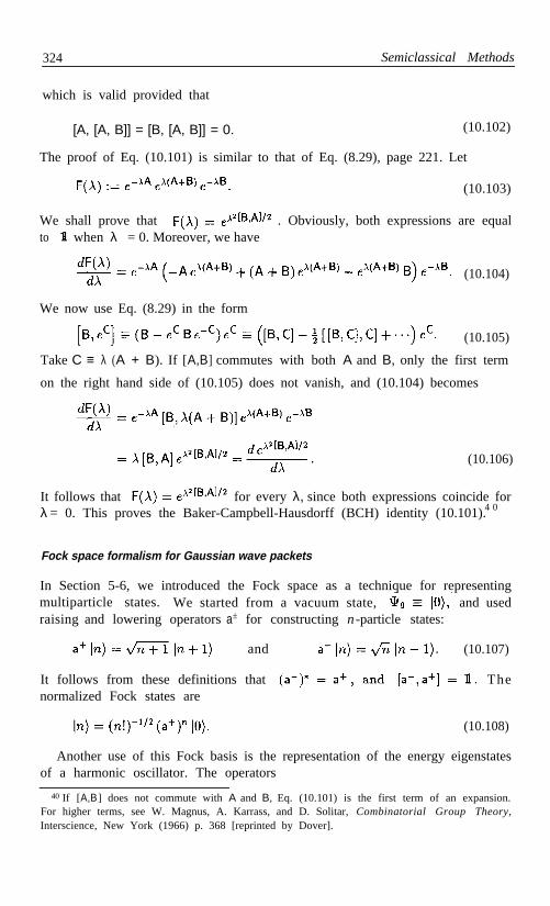
324
which is valid provided that
Semiclassical Methods
[A, [A, B]] = [B, [A, B]] = 0. (10.102)
The proof of Eq. (10.101) is similar to that of Eq. (8.29), page 221. Let
(10.103)
We shall prove that . Obviously, both expressions are equalto when λ = 0. Moreover, we have
(10.104)
We now use Eq. (8.29) in the form
(10.105)
Take C ≡ λ (A + B). If [A,B] commutes with both A and B, only the first term
on the right hand side of (10.105) does not vanish, and (10.104) becomes
(10.106)
It follows that for every λ, since both expressions coincide forλ = 0. This proves the Baker-Campbell-Hausdorff (BCH) identity (10.101).4 0
Fock space formalism for Gaussian wave packets
In Section 5-6, we introduced the Fock space as a technique for representingmultiparticle states. We started from a vacuum state, and usedraising and lowering operators a± for constructing n -particle states:
and
It follows from these definitions thatnormalized Fock states are
(10.107)
The
(10.108)
Another use of this Fock basis is the representation of the energy eigenstatesof a harmonic oscillator. The operators
40 If [A,B] does not commute with A and B, Eq. (10.101) is the first term of an expansion.For higher terms, see W. Magnus, A. Karrass, and D. Solitar, Combinatorial Group Theory,Interscience, New York (1966) p. 368 [reprinted by Dover].

Coherent states 325
and (10.109)
satisfy [x, p] = The ground state of the Hamiltonian is
(10.110)
It satisfies Note that The n -th energylevel is The corresponding eigenstate will be denoted by n⟩.
We can now write the Gaussian wave packet (10.99) in terms of these Fockstates. We shall label this wave packet by its shift parameters, and denote it as
Recalling that represents a translation by x′ , we have
(10.111)
By virtue of the BCH identity (10.101), this can also be written as
(10.112)
The first exponential on the right hand side of (10.112) is an irrelevant phase andmay be discarded. In the second one, we introduce a complex shift parameterα by writing, as in Eq. (10.109),
and (10.113)
We thus have
(10.114)
The expression
(10.115)
is called the displacement operator. The state (10.112) can now be written as
(10.116)
It is called a coherent state. 41 Note that it has the same dispersion σ² as theground state 0 ⟩. Different values of σ can be achieved by an operation calledsqueezing, which has important applications in quantum optics.4 2
Exercise 10.22 Prove the following relationships:
(10.117)
(10.118)
(10.119)
4 1 R. J. Glauber, Phys. Rev. 131 (1963) 2766.42 Nonclassical Effects in Quantum Optics, ed. by P. Meystre and D. F. Walls, Am. Inst.
Phys., New York (1991).

326 Semiclassical Methods
(10.120)
(10.121)
(10.122)
(10.123)
The last equation is often taken as the definition of a coherent state.
Overcomplete basis
The Fock states n ⟩ form a complete orthonormal basis: any state ψ can bewritten in a unique way as , where = 1. It will now beshown that the coherent states α ⟩ can also be used as a basis. That basis isnot orthogonal and it is overcomplete, but it is nonetheless possible to obtain,for each ψ, a representation , where
(10.124)
Moreover, this representation is unique if we impose suitable restrictions on theadmissible functions c(α ).
In the proof given below, I follow Glauber’s lucid paper41 and use, as in thatpaper, Dirac’s bra-ket notations (see Table 3-1, page 78). For example, thecompleteness of a sum of projectors is expressed by Likewise,with coherent states, we shall see that
(10.125)
so that the set of operators forms a POVM, as in Eq. (9.81). Thisidentity follows from
(10.126)
which is easily proved by writing α = r eiθ , and d ² α = r d r d θ. From thedefinition of a coherent state in Eq. (10.118), we have
(10.127)
whence Eq. (10.125) readily follows.Let us now expand an arbitrary state ψ . In the Fock basis, we have
(10.128)

Coherent states 327
which defines the coefficients cn = . Likewise,
(10.129)
where use was made of Eq. (10.118). Let us now introduce a complex variablez and define a function
(10.130)
where cn = . This function is analytic in every finite region of the z plane(it is called an entire function). We thus have
(10.131)
Conversely, it is possible to obtain for the entire function an explicitformula similar to cn = . We have
(10.132)
where use was made of Eq. (10.121). Next, we note that, for any integer n,we have . This follows from Eq. (10.126) and from theexpansion . A more general form of this identity is
(10.133)
and Eq. (10.132) gives
(10.134)
Exercise 10.23 Show that if , then
Note that is in general different from
Exercise 10.24 Show that, for all positive integers n,
(10.135)
Hint: Expand in powers of α and use Eq. (10.126).
(10.136)

328 Semiclassical Methods
In spite of the fact that the coherent states α ⟩ are not linearly independent,the Glauber expansion (10.131) is unique, because the functions whichappear in the coefficients are required to be smooth, entire functions of . Forexample, the trivial identity is not a valid Glauberexpansion. The correct way of expanding a basis vector is
(10.137)
The coefficient is considerably smoother than . Shallwe get an even smoother result by iterating this procedure? Let us try:
(10.138)
Integration over β g i v e s , as in the right handside of (10.137): there is no further spreading. The expansion is unique.
It is likewise possible to define a coherent representation of operators, b yusing their matrix elements . More details and various applications toquantum optics can be found in Glauber’s article41 and in the bibliography atthe end of this chapter.
Angular momentum coherent states
It is natural to seek generalizations of the minimum uncertainty wave functionin Eq. (10.99) to sets of noncommuting operators other than q and p. F o rexample, we may want all three components of angular momentum to havesmall dispersions . The sum of these dispersions is, for a given totalangular momentum,
(10.139)
To find the minimum value of this expression, let us rotate the coordinatesystem so that the new z' -axis is parallel to the vector ⟨ Jk⟩
= 0. The maximum value of. We then have
is J 2 . Therefore, the sum of thedispersions in Eq. (10.139) is minimal for states that fulfill
(10.140)
with the unit vector n parallel to any given ⟨ J k ⟩. This equation defines angularmomentum coherent states,43,44 which have the property
(10.141)
In particular, and in any direction perpendicular to n.43 J. M. Radcliffe, J. Phys. A 4 (1971) 313.44 P. W. Atkins and J. C. Dobson, Proc. Roy. Soc. A 321 (1971) 321..

Coherent states 329
These coherent states will be denoted by θ,φ⟩ , where θ and φ are the polarand azimuthal angles of n. Note that θ,φ⟩ can be obtained fromby rotating that state through Euler angles φ around the z -axis, and then θaround the new y -axis. Therefore,45
(10.142)
Let us evaluate . We first perform the integration over φ,which gives , and we are left with
(10.143)
The integral on the right hand side is recognized as a beta function, which isequal to 2(j + m )!(j – m )!/(2j + 1)!. We thus obtain
(10.144)
We shall soon see that this is a special case of a more general formula, valid forany group.
Exercise 10.25 Show that
(10.145)
and
(10.146)
where Θ is the angle between the directions (θ' , φ ') and (θ" ,φ").
The angular momentum coherent states have many properties similar tothose of the harmonic oscillator coherent states,46 because they are related tothe latter by the group contraction that was discussed on page 322.
45M Tinkham, Group Theory and Quantum Mechanics, McGraw-Hill, New York (1964).p. 110.
46F. . Arecchi E. Courtens, R. Gilmore, and H. Thomas, Phys. Rev. A 6 (1972) 2211.T

330 Semiclassical Methods
Coherent states for any group
The above considerations can be generalized to any group.47 Consider a set Sof N unitary matrices U α having the properties of a group: S includes the unitmatrix 1, the inverse of any Uα ∈ S, and the product U γ = UβUα of anytwo members of S.
For any fixed consider the states The sum
has the property that, for any U β ,
(10.147)
(10.148)
because the set of all Uγ = U βUα (for fixed Uβ , and for all Uα ∈ S ) contains Ndifferent matrices, and therefore it runs over all the elements of S.
It follows from (10.148) that UβA = AUβ for all the Uβ of the group. There-fore, if the matrices Uβ are an irreducible representation of that group, we have,by virtue of Schur’s lemma, A = c1. Taking the trace of (10.147), we obtaincd = = N, where d is the dimensionality of H. It follows that
(10.149)
The matrices (d/N) thus are members of a positive operator-valuedmeasure (POVM), as in Eq. (9.81).
These definitions can be extended to continuous groups, once a suitable mea-sure is defined to replace the discrete sum over α . For example, the Uα maybe the ordinary rotation matrices of order d = 2j + 1. The then arethe coherent states that were discussed earlier. In this case, N becomes
, and we obtain again Eq. (10.144).
10-8. Bibliography
D. Park, Classical Dynamics and its Quantum Analogues, Springer, Berlin(1990).
W. Dittrich and M. Reuter, Classical and Quantum Dynamics: from ClassicalPaths to Path Integrals, Springer, Berlin (1992).
These textbooks compare many aspects of classical and quantum mechanics thatwere not discussed in the present chapter. The first one contains numerous exercises,making it ideal for independent study.
47A. M. Perelomov, Comm. Math. Phys. 26 (1972) 222.

Bibliography 331
Path integrals
R. P. Feynman and A. R. Hibbs, Quantum Mechanics and Path Integrals,McGraw-Hill, New York (1965).
L. S. Schulman, Techniques and Applications of Path Integration, Wiley,New York (1981).
M. S. Marinov, “Path integrals in quantum theory: an outlook of basicconcepts,” Phys. Rep. 60 (1980) 1.
Wigner functions
M. Hillery, R. F. O’Connell, M. O. Scully, and E. P. Wigner, “Distributionfunctions in physics: fundamentals,” Phys. Rep. 106 (1984) 121.
Coherent states
J. R. Klauder and B.-S. Skagerstam, Coherent States, World Scientific,Singapore ( 1985).
A. Perelomov, Generalized Coherent States and their Applications, Springer,Berlin (1986).
Recommended reading
S. A. Hojman and L. C. Shepley, “No Lagrangian? No quantization!”J. Math. Phys. 32 (1991) 142.
The authors prove that the canonical commutation relations are compatible withspecified equations of motion only if the latter are equivalent to the Euler-Lagrangeequations derived from some Lagrangian L (this Lagrangian need not be unique).
I. V. Aleksandrov, “The statistical dynamics of a system consisting of aclassical and a quantum subsystem,” Z. Naturf. 36 a (1981) 902.
This is an interesting attempt to construct a hybrid system, partly classical andpartly quantum mechanical. Each element of the quantum density matrix is a Liouvillefunction of the classical dynamical variables. The equation of motion involves both
a commutator and a Poisson bracket with the same Hamiltonian. The normalizationTr ( ρ) dqdp = 1 is invariant. Unfortunately, there is no guarantee that ρdqdp
always remains a positive operator, or that Tr ρ ≥ 0 for every value of q and p. It thusseems that this hybrid formalism cannot have a consistent physical interpretation.
L. E. Ballentine, Quantum Mechanics, Prentice-Hall, Englewood Cliffs (1990)Chapt. 15.
R. G. Littlejohn, “The Van Vleck formula, Maslov theory, and phase spacegeometry,” J. Stat. Phys. 68 (1992) 7.

Chapter 11
Chaos and Irreversibility
11-1. Discrete maps
Most dynamical problems have no known analytic solution. In some cases,approximation methods such as perturbation theory give satisfactory answers.However, it often happens that the only available approximation is the useof numerical methods. Thanks to the advent of fast computers, numericalsimulations have become a readily available tool, and they may have a highdegree of reliability—if correctly used.
In a computer simulation, continuous physical quantities, time in particular,are replaced by discrete surrogates. l This naturally suggests to investigate theproperties of dynamical models which are intrinsically discrete, but still obeysome of the ordinary laws of physics. For instance, in quantum mechanics,we may have, instead of the continuous evolution generated by Schrödinger’sequation, a discrete sequence of unitary transformations. In classical mechanics,the mapping q(t), p (t) → q(t + δ p(t + δt) will proceed by discrete steps,t ),each one of which is required to be a canonical transformation. These discretemappings are akin to a sequence of stroboscopic views taken during a continuousevolution, and they share many of the properties of the latter. In the presentsection, we shall discuss classical (canonical) discrete dynamics, as a preparationto the study of quantum mechanical discrete maps.
Transfer matrices
To simplify notations, let r := q1 .. . q n , p1 . . . p n denote a point in the 2n-dimensional phase space. The problem in which we are interested is whetherthe orbit r (t) is stable, or unstable, with respect to small perturbations of theinitial conditions. This issue can be investigated by considering the behavior of
1Some authors have proposed that time and space are fundamentally discrete, with unitsof the order of 1.6 × 10 - 3 5 m, where G is Newton’s gravitational constant. Thepresent discussion has nothing to do with these speculations. At the time of writing, there isno satisfactory quantum theory of gravity.
332

Discrete maps 333
a small deviation, r → r + ∈ z. We shall see that it obeys Eq. (11.6) below.Let us write Hamilton’s equations of motion (for continuous time) as
(11.1)
where
(11.2)
is a symplectic matrix. Consider a small deviation, . To first orderin ∈ , we have, from Eq. (11.1),
(11.3)
This is a linear equation for the deviation vector z k . Note that there is adifferent matrix M ik (t) for each orbit.
Exercise 11.1 Show that the matrix
(11.4)
satisfies
and (11.5)
The linear equations (11.3) can in principle be integrated, with a result
z(t) = S(t)z(0). (11.6)
The transfer matrix S (t) satisfies = S M and S (0) = 1. Transfer matricesplay in classical mechanics a role similar to that of unitary matrices in quantummechanics. However, some of their properties are radically different.
Consider two different deviations, y and z. The symplectic area which theyspan in phase space is ηz (where denotes a row vector which is the transposedof y ). This area is a constant of the motion, because
(11.7)
where use was made of Eqs. (11.3) and (11.5), and a tilde denotes a transposedmatrix. It follows that
(11.8)
and therefore
(11.9)

334 Chaos and Irreversibility
The transfer matrix S thus belongs to the symplectic group (the group of trans-formations which leave the symplectic matrix η invariant).
Exercise 11.2 Show that Det S = 1 and therefore that the volume of a smallelement of phase space remains invariant under the transformation (11.6).
Exercise 11.3 Show that the area preserving theorem holds for any canonicaltransformation.
An important property of symplectic matrices is that their eigenvalues arepaired as λ and λ –1 . Proof: Let S v = λ v. We then also have S –1 v = λ –1 v,and we obtain from Eq. (11.9), which can also b written as
(11.10)
Therefore η v is an eigenvector of , belonging to the eigenvalue λ - 1. But Sand have the same set of eigenvalues, since they have the same characteristicequation. Therefore all these eigenvalues are paired, as λ and λ- 1 .
Moreover, since S is real, its complex eigenvalues are also paired as λ and Therefore they come either as conjugate pairs on the unit circle, or as quartets,
Periodic orbits
If a solution of Hamilton’s equations (11.1) satisfies r(t + T) = r (t), the orbit issaid to be periodic, with period T. This notion can be extended to any discretemap. Consider a nonlinear transformation, r → F (r), where F is an invertiblecontinuous function, so that neighboring points are mapped onto neighboringpoints. We have
(11.11)
For some particular r 0 , this sequence may be periodic, namely rN = r 0 . Wethen say that r0 is a fixed point of order N.
We shall mostly be interested in the case where the map F is a canonicaltransformation. For example, F(r) may be the result of integrating Hamilton’sequations (11.1), either for a prescribed time or, more commonly, until the orbitr(t) reaches a prescribed surface (or higher dimensional manifold). The latteris called a Poincaré surface of section. Let r0 be a fixed point on that surfaceof section. Since F(r0 ) is continuous, a neighboring point on the samesurface, is mapped onto , where . Here, the matrix S refers toa complete period. This matrix is in general a function of r0. It belongs to thesymplectic group, because the area preserving theorem is valid for all canonicaltransformations.
The stability of a periodic orbit is determined by the eigenvalues of S. Afterk turns (that is, kN steps), the orbit which started at will pass through
. Let us write z0 as a linear combination of eigenvectors,

Discrete maps 335
(11.12)
where Vλ is the eigenvector of S corresponding to eigenvalue λ . We then have
(11.13)
Let Λ denote the largest eigenvalue of S. If Λ is real, the asymptotic behaviorof z k for large k is an exponential growth, . We shall call Λ the Lyapunov factor of the periodic orbit. (If time is continuous, Λ is usuallywritten as e L T, and L is called the Lyapunov exponent.) More generally, thelargest eigenvalues of S may come as conjugate pairs (where Λ and θare real). We then have, asymptotically, , so that theexponential growth is modulated by periodic oscillations. In all these cases, theorbit is clearly unstable. It is only when all the eigenvalues of S lie on the unitcircle that a periodic orbit is stable.
KAM manifolds
It will now be shown that, in a 2m-dimensional surface of section, all the pointslie on m quadratic manifolds
(11.14)
This is illustrated in Fig. 11.1 for the simple case of a fixed point of order 1on a 2-dimensional surface of section (m = 1): the points z 0 . . . z 3 lie on anellipse, if the orbit is stable. They would lie on a hyperbola in the case of anunstable fixed point.
Fig. 11.1. An elliptic fixed pointr0 is located at the origin of a2-dimensional surface of section.Consecutive points of a neighbor-ing orbit, , lie on an ellipse.
To prove this property, consider Eq. (11.13) for any given value of k. Writethe 2m values of λ k as an array, x λ , and the 2m components of z k as anotherarray, yµ . The result has the form of a linear transformation:
(11.15)

336 Chaos and Irreversibility
where A µλ is the µth component of cλv λ in the expansion of z0 in Eq. (11.12).By inverting (11.15), we obtain , where B is the inverse matrixof A. Recall now that the 2m values of λ are paired, as λ and , so thatthe 2m values of x λ ≡ λk are also paired: x λx λ ' = 1. It follows that
(11.16)
which is just another way of writing Eq. (11.14).The physical interpretation of this result is a conservation law: in the vicinity
of the fixed point r0 , there is some function of r (that is, of q and p) which isconstant, and Eq. (11.14) represents the first terms in a power expansion of thisfunction. However, some care is needed here, and various possibilities must bedistinguished.
For a stable (also called elliptic) fixed point, the sequence of z k may denselycover a closed manifold C. This is an ellipse (or ellipsoid) if the zk are infini-tesimal, a more complicated manifold if they are finite. In particular, for thesimple case of a 2-dimensional surface of section, C is a closed curve whichdivides the surface of section into two parts. If an initial point r is inside thedomain bounded by C, all the consecutive mappings of r will also be inside,by continuity. (Proof: let a continuous curve R connect the fixed point r0 tor0 + z 0 and pass through r. Consecutive mappings of R will connect r0 tor 0 + z k without ever leaving the domain bounded by C.)
In the general case of a finite deviation z, the existence of such a manifold isguaranteed, under appropriate conditions, by the KAM theorems.2–4 Considera n integrable Hamiltonian system, namely one with n analytic constants ofmotion in involution. The orbit of r then lies on a n -dimensional torus in the2n-dimensional phase space. If that Hamiltonian is perturbed in a way whichmakes it nonintegrable, there will be fewer than n constants of integration(there may remain only one, the energy). The KAM theorems assert that if theperturbation is analytic, or at least differentiable sufficiently many times, thesetori will be distorted but they will not disappear as long as the perturbation issmall enough. [This property apparently holds under less restrictive conditions,such as for the nonanalytic law of force (11.20) discussed below, but there isno formal proof.] As the perturbation increases, the KAM manifolds graduallybreak down, and the motion of a point r in phase space can explore domainsof dimensionality higher than n (up to 2n – 1 dimensions, if energy is the onlyremaining constant of motion of the perturbed Hamiltonian).
The situation is more complicated in the case of an unstable (or hyperbolic)fixed point. In the simplest case of a 2-dimensional surface of section, it mayhappen that there exists a continuous curve which behaves as a hyperbola inthe vicinity of the unstable fixed point, and which is mapped onto itself by
2 A. N. Kolmogorov, Dokl. Akad. Nauk 98 (1954) 527.3 V. I. Arnol’d, Usp. Mat. Nauk 18 (1963) 13 [transl. Russ. Math. Surveys 18 (1963) 9].4 J. Moser, Nachr. Akad. Wiss. Göttingen, Math. Phys. K1 (1962) 1.

Discrete maps 337
the nonlinear transformation r → F( r ). However, in the generic case, thesequence of z k wanders over all accessible parts of the surface of section thatcan be reached without crossing a KAM line. Such a motion is called irregularor chaotic , because it becomes effectively unpredictable for long times: theslightest perturbation of the initial conditions is amplified, step after step, untilany computer with finite resources is unable to determine new points in a reliableway. The situation is illustrated by Fig. 11.2, which displays both KAM linesand chaotic areas.
That figure also shows chains of islands of stability, namely KAM lines whichconsist of several disjoint parts. The latter arise whenever a mapping such asthe one sketched in Fig. 11.1 does not densely cover a closed curve, but containsonly a finite number of points, because it is itself periodic: z s = z 0 . Each one ofthese points thus is a fixed point of order s. If this new periodic orbit is stable,the associated KAM line consists of s disjoint parts.
Case study: area preserving map on a torus
Consider a compact 2-dimensional phase space, –1 ≤ q,p ≤ 1. The end points–1 and 1 are identified. The discrete map consists of two steps, namely
q → q' = q + p (“mod 2”), (11.17)
followed by
p → p' = p + f (q') (“mod 2”). (11.18)
Here, “mod 2” means that if | q' | or | p ' | exceeds 1, one must add or subtractan integral multiple of 2 to bring it back to the domain [–1, 1]. This map isinvertible, by p = p' – ƒ(q'), followed by q = q' – p.
Exercise 11.4 Show that this transformation is canonical:
(11.19)
As a simple case, consider the quadratic law of “force” 5
(11.20)
We shall give the name parabolic map to the resulting law of motion. The pointq = p = 0 obviously is a first order fixed point of this map. In its vicinity, themap can be linearized as
5 This is a poor man’s version of the standard map with ƒ = – K sin(q/ π), about which thereis a vast literature. The quadratic law (11.20) is used here for pedagogical reasons, because itallows a detailed investigation with minimal computing tools, as shown in the Appendix.

338 Chaos and Irreversibility
q' = q + p, p' = p – q' = – q . (11.21)
The corresponding transfer matrix has eigenvalues
Exercise 11.5 Find the form of the KAM ellipse corresponding to (11.21).
Exercise 11.6 Show that the point q = ±1, p = 0 is an unstable fixed point,and that the eigenvalues of the transfer matrix are λ = (3 ± )/2.
Some complete orbits of the parabolic map are displayed in Fig. 11.2. Asexpected, there are concentric elliptic KAM lines in the vicinity of the stable
Fig. 11.2. The parabolic map is illustrated here by 13 regular orbits and onechaotic orbit. The vertical axis is –1 < p < 1, and the horizontal axis is–1 < q < 1. The regular orbits start at p = 0 and q = 0.05,..., 0.65. Thechaotic orbit explores most of the phase space (10 6 points were plotted).

Discrete maps 339
fixed point q = p = 0. The shape of these closed curves becomes more com-plicated as their size grows. They occasionally break up into chains of islandsof stability, corresponding to higher order fixed points. Further away from theorigin, most of phase space is covered by a chaotic region, where blank areasindicate the presence of additional islands of stability.
In the chaotic region, nearly all the periodic orbits have Lyapunov factorsΛ > 1. Therefore an infinitesimal region of phase space is stretched, after ksteps, by a factor Λk (in the limit k 1). For a finite region, the situation ismore complicated, because both Λ and the direction of the eigenvector v∧ varyfrom point to point. This causes the finite region to be distorted in a grotesqueway, projecting increasingly long and thin filaments, as illustrated in Figs. 11.3
Fig. 11.3. An initially circular domain, entirely within the chaotic region ofthe parabolic map, is shown after 3 and 6 steps. Note that the area of thisdomain is conserved, while its shape becomes more and more distorted. ThePOST SCRIPT program which draws this figure is given in the Appendix.

340 Chaos and Irreversibility
and 11.4. As the number of iterations tends to infinity, these filaments willpass arbitrarily close to any point which can be reached without crossing aKAM line. This property is called ergodicity (the label “ergodic” is sometimesrestricted to situations where the entire energy surface can be reached).
Ergodicity and mixing
In the present context, ergodicity is almost tautological because any regionwhich would not be covered by these chaotic filaments would necessarily havea boundary, invariant under the dynamical map, and then this boundary itselfwould be an impenetrable KAM line. There is however a nontrivial and muchstronger property, called mixing, which has profound consequences.
Fig. 11.4. The same circular domain, after 12 steps of the parabolic map.When many additional steps are executed, the increasingly long and thinfilaments will pass arbitrarily close to every point of the chaotic region.

Irreversibility in classical physics 341
Consider a compact region R 0 of phase space, such as the small circle inthe preceding figures, and let R k be its k th iteration by the mapping underconsideration. Let µ be the ratio of the volume of R 0 to the total volume ofthe accessible region which is covered by the successive iterations Rk . Then, ask → ∞, every accessible fixed region of phase space will have the same fractionµ of its volume covered by points belonging to Rk . Seen on a coarse scale,the entire accessible region of phase space is uniformly covered by R∞ . Thenotions of mixing and coarse graining are essential in the derivation of classicalirreversibility.
11-2. Irreversibility in classical physics
The intuitive meaning of “irreversibility” is that there are dynamical evolutionswhich can easily be prepared, but it is extremely difficult (we say “impossible”)to prepare the time-reversed evolutions. For example, it is easy to get a cup oflukewarm water by placing a cube of ice in a cup of boiling water, and waitingone hour, say. It is impossible to prepare a cup of lukewarm water in such away that, one hour later, it will turn into an ice cube floating in boiling water.
The classical explanation given to irreversibility is based on the concepts ofmixing and coarse graining. Mixing, whose intuitive meaning was illustrated inFig. 11.4, is a property which can be proved rigorously, in the limit t → ∞, forsome specific physical systems, such as a gas of hard spheres ( i.e., impenetrable,nonrotating spheres, which rebound elastically when they collide). Formally, itmeans the following:6 Consider two finite (and fixed) regions of phase space, V 1
and V 2 , which are not dynamically separated by an isolating constant of motion(or a closed KAM manifold), and whose measures are fractions µ1 and µ2 ofthe total accessible phase space. Suppose that the Liouville density ƒ1( q ,p ) isuniform in V1 at time t l , with The dynamical evolution causesthis density to become ƒ2(q , p ) at time t2 . Then, for any t2 sufficiently remotefrom t1 (in the future or the past) and for sufficiently large µ 1 and µ 2 , wehave irrespective of where V1 is. The system appears to haveno memory of its origin. Obviously, the smaller µ 1 or µ2 , the larger the time
needed for mixing. (I consider only finite times, not the unattainablemathematical limit of infinite time.) Notice that the mixing property is timesymmetric. By itself it cannot explain irreversibility.
In the ice-cube paradigm, V1 (the region of phase space which corresponds toan ice cube in boiling water) is considerably smaller than V2, which correspondsto what we loosely call “lukewarm water” with no further specification of thewater properties. This is because, for a given total energy, nearly all the pointsof phase space are compatible with this vaguely specified state of water, so that
Therefore, almost every dynamical evolution will lead to lukewarm
6 V. I. Arnold and A. Avez, Ergodic Problems in Classical Mechanics, Benjamin, New York(1968) pp. 19–22.

342 Chaos and Irreversibility
water, with extremely small inhomogeneities, since is the probabilityof finding the final state in V2 . Nevertheless, we can, conceptually, preparelukewarm water at time t2 so that, at a later time t1 it will separate into an icecube and boiling water. However, this requires a very special preparation: notjust any cup of lukewarm water, but one with precise correlations between all themolecules. This preparation is restricted to lie in an exceedingly contorted regionof phase space, far more complicated than Fig. 11.4, and with structural detailsso small that mixing, as defined above, will not yet have been accomplishedafter the given finite time t1 – t 2 .
Now comes coarse graining: we are unable, with our imperfect instruments,to coerce the initial state to reside within a region of phase space which is sosmall, or with a structure so complicated, that mixing will not yet have occurredafter a finite time t1 – t2 . That is, we cannot prepare the system at time t2 sothat, after a finite time t1 – t2 , it will be located with certainty in the desireddomain V 1 of phase space. There are evolutions (such as from lukewarm waterto an ice cube in boiling water) which cannot be made to proceed.
Deceptive irreversibility
The above argument deserves close scrutiny. The claim that “we are unable toachieve such a preparation” ought to be proved. What is the degree of difficultywhich is called “impossible”? (How, indeed, do we measure difficulty?) Oneshould never underestimate the skill of experimental physicists. For instancethe spin echo 7,8 phenomenon shows that an apparently irreversible behaviorcan, under appropriate circumstances, be reversed. In that experiment, a largenumber of spins, initially aligned, acquire random phases under the influenceof random, unknown, but fixed internal fields, acting during a known time t. Asuitable RF pulse can then invert all these phases and, after the same time t,all the spins are again aligned. This is possible because all the spin precessionsare decoupled from each other. Their equations of motion are integrable. Thephases appear random to the untrained eye, but actually they are correlated.They are similar to a text which has been encrypted by a secret key, appearsincomprehensible, but can be decrypted by anyone knowing the key. Informa-tion is not destroyed by encryption, it is only made less accessible. Likewise, inthe spin echo case, the “key” is the strength of the RF pulse which inverts thephases and realigns the spins.
To give a quantitative measure to these concepts, the notion of logical depthwas introduced by Bennett.9 It is, roughly speaking, the number of elementarylogical steps needed to obtain the value of a physical quantity from the minimalprogram which can compute it. Unfortunately, logical depth itself is not com-putable: this is due to the most fundamental property of computability theory,
7 E. L. Hahn, Phys. Rev. 80 (1950) 580.8 J l Rothstein, Am. J. Phys. 25 (1957) 510.9 C. H. Bennett, in Emerging Syntheses in Science, ed. by D. Pines, Addison-Wesley, Reading
(1987) p. 215.

Irreversibility in classical physics 343
namely the unsolvability of the halting problem.10,11 Moreover, the length of acomputation can sometimes considerably decrease if the minimal program whichgenerates it is replaced by a longer, but more efficient program. Nevertheless,if we set some arbitrary rate of exchange between run time and program size,the resulting logical depth can be shown to be roughly machine-independent.9
Exercise 11.7 The Kac ring model 12,13 consists of n equidistant balls on thecircumference of a circle. Each ball can be either black or white. Moreover, mmarkers are placed on the circumference, in a random way, at fixed positions.All the balls move clockwise with the same velocity and, when a ball passes amarker, its color changes. The initial color distribution is given (for example,all the balls are white). The problem is to find the color distribution after along time. (Assume n >> m >> 1.)
In the above exercise, we intuitively expect a monotonic approach to anequilibrium state, with equal numbers of white and black balls, except for smallfluctuations. This is indeed what happens at the beginning of the motion.Yet, this cannot continue forever. The system is manifestly periodic, becauseafter two complete turns each ball is back to its original color, having passedeach marker twice. Here again, the colors of the balls may look random to theuntrained eye, but they are strictly correlated: the encryption key is the fixeddistribution of markers.
Let us now imagine that an observer starts to watch the n black and whiteballs only a short time before the end of a complete cycle. Their color distri-bution, which initially appears random, spontaneously evolves from disorder toorder, until all the balls are white; and thereafter, they return to a pseudo-random state. The baffled observer will perhaps try to interpret his findings asa statistical fluctuation, one which would have very low a priori probability. (Ifa cup of lukewarm water turned into an ice cube in boiling water, this wouldbe called a miracle, for sure.)
However, upon closer analysis, our observer would realize that he has been thevictim of a conspiracy: the apparently random distribution of white and blackballs is logically deep. It has been cleverly contrived by means of a complicatedcalculation, or a long physical process. To orchestrate this result, the preparerwould first have to produce m pseudo-random numbers (the markers positions,between 0 and 2π) and then to count, for each one of the n balls, how manyof these pseudo-random numbers fall between 2πk /n (the initial position of thekth ball) and 2π( k+l )/n (its position after l steps). Recall that n >> m >> 1, sothat a lot of computation is necessary in order to produce the fake “statisticalfluctuation” which mimics a spontaneous decrease of entropy.
1 0
11A. M. Turing, Proc. London Math. Soc. 42 (1936) 230.M. Davis, Computability and Unsolvability, Dover, New York (1982).
12
1 3M. Kac, Probability and Related Topics in Physical Sciences, Interscience, New York (1959).M. Dresden, in Studies in Statistical Mechanics, ed. by J. De Boer and G. E. Uhlenbeck,
North Holland, Amsterdam (1962) Vol. I, p. 316.

344 Chaos and Irreversibility
Computational complexity
Likewise, consider the evolution of a nonintegrable dynamical system. Eventhough this system is deterministic, its long time behavior is effectively chaoticbecause, as we shall now see, the amount of computation required to predict themotion increases faster than the actual duration of the motion itself. Therefore,for sufficiently long times, no computer with finite resources will be able topredict the final state of the system, except statistically. Chance is supreme.The final state is “random” and the evolution is “chaotic.”
A quantitative measure for the computational work needed to accomplish agiven task is its computational complexity. 14 This notion is defined in roughlythe same way as logical depth, but it refers to a process (such as a dynamicalevolution) while logical depth is a property of the end product of such a process.For instance, let us evaluate the computational complexity of a classical chaoticorbit in a bounded system. That orbit, C, will eventually pass near its initialpoint. There must therefore be an exactly periodic orbit, O with a startingpoint very close to that of C (and with a Lyapunov factor Λ > 1). let be theinitial separation of these orbits. After k turns, their separation will be aboutΛk ∈ , provided that this still is small enough to allow the use of the linearizedequations of motion (11.3). Conversely, in order to predict the final point of Cwith a precision ∈, the initial point must be specified with a precision Λ– k ∈.
The number of digits to be specified in the initial data thus increases linearlywith the duration of the physical motion that we want to compute.15 This aloneis sufficient to cause the computational complexity to increase, for t → ∞, fasterthan t log t, because there surely are some multiplications in the computation,and the best (currently known) algorithm
14for multiplying two numbers with
N bits (N >> 1) qre uires a number of elementary logical operations whichincreases faster than N log N. In practice, the computational complexity willincrease considerably faster than that, if the computation involves a sequenceof iterations, such as in the Runge-Kutta method. The numerical error for astep of duration τ typically behaves as aτ n where a depends on the system ofequations (not on τ ) and n is a small integer. Optimally, the expected numericalerror due to the iterative algorithm should be about the same as the admissibleround-off error, namely Λ– t / T∈ , where t is the time remaining until the end ofthe motion, and T is the period of the neighboring orbit . The required τ thusbehaves as Λ- t/nT , and the total number of steps as Λ t / n T
. The computationalcomplexity of a classical chaotic orbit thus increases exponentially with theduration of the motion.
Admittedly, this conclusion was reached by assuming the use of an iterativealgorithm of the Runge-Kutta type. For any specific problem, more efficientsmethods may exist. However, if the computational complexity of the fastest
1 4G. Brassard and P. Bratley, Algorithmics: Theory and Practice, Prentice-Hall, EnglewoodCliffs (1988).
1 5 Recall that the magnitude of a number is an exponential function of the number of digitsneeded to represent it.
O

Irreversibility in classical physics 345
algorithm can be shown to increase more rapidly than the actual duration ofthe motion, no long range predictions are possible, and the system is chaotic.
Are these difficulties subjective?
We must exert extreme caution before claiming that it is impossible to achievea specific goal, just because it looks difficult. In the case of the spin echo, orthe Kac model, what appeared at first sight difficult became easy under closeranalysis. Likewise, consider the intricate phase space domain in Fig. 11.4. Sinceit was obtained by a canonical mapping, there must be some canonical variableswith which that domain has a simple shape, while the initial circular domainappears utterly distorted and complicated.
These two coordinate systems are canonically equivalent, but they are notequivalent from the point of view of physics. There are privileged coordinates,namely those in which the observer and his instruments have a simple shapewhich can be specified by a short description. Given such a privileged coordinatesystem, it is objectively difficult—but not formally impossible—to prepare aninitial state lying within a contorted domain, as in Fig. 11.4, with extremelyfine structural details. This is because the extreme precision which is requirednecessitates the handling of a large amount of information, at the very leastsupplying many digits in the initial data. The process of getting and recordingthis information dissipates at least an equivalent amount of entropy in the restof the world (see page 266). However, if the accessible part of the universe isfinite, there must be an upper limit to the entropy that we can generate in it:our computing ability may be large, but it is not infinite.
It thus appears that some physical properties are subjective and depend onour intellectual and experimental skills. The spin echo phenomenon, discussedabove, is an example: where most people would see only disorder (high entropy),others may recognize a perfectly ordered (but logically deep) state, with zeroentropy. This subjectivity should not be a matter of concern, as long as we ad-mit that there is some limit to our skill. The precise limit has little importance:our description of physical phenomena is almost indifferent to where this limitis set, because the Lyapunov exponent which rules the dynamical evolution ofa macroscopic system is so huge that it will overcome, within an exceedinglybrief time, even the most extravagant claims of computability and reversibility.
The role of the environment
Irreversibility results from our accepting that there are things that we cannot do.We should not, however, underestimate our ability. As shown by Hahn’s spin-echo 7 experiment, macroscopic observers are not restricted to coarse-grainedvariable. 1 6 If our goal is motion reversal, we don’t have to measure a velocityin order to reverse it—a mundane elastic bounce will do that job. In a large
16 J.M.Blatt, Prog. Theor. Phys. 22 (1959) 745.

346 Chaos and Irreversibility
system, a reversal of all the velocities does not imply a measurement of allthe velocities (which would indeed be impossible for a macroscopic observer).Therefore, “proofs” of irreversibility based on a vaguely defined coarse-grainingare not really convincing, and further considerations are needed.
Irreversibility would still occur if there were no limit to our resolving power,and if any state specified by a finite algorithm could be prepared experimentally.(We already made such optimistic assumptions when introducing the quantumsuperposition principle, page 50.) The fundamental limitation to an observer’sability is of a different nature: he must restrict his observations to a finite partof the Universe. Insurmountable difficulties do not arise from having to handlelarge, complicated systems; rather, they appear with limited and not perfectlyisolated systems.
1 6
It is sometimes claimed that physical systems can be isolated as well as wewish, and that it is only a matter of technological skill to reduce the influence ofthe external world to an arbitrarily low level. To show the fallacy of this claim,let us for a moment imagine that this external world is completely known to us,and let us examine how it would affect the system under consideration. In theequations of motion, the external world would appear as additional degrees offreedom, weakly coupled to the degrees of freedom of the original system. Thecoupling being very weak, one could legitimately ignore the global energy trans-fer between the internal and external degrees of freedom (e.g., superconductingcurrents have been shown to run for an “infinite” time, on a human scale).However, the detailed microscopic behavior of a chaotic system is appreciablyaffected by its weak coupling with the external world much more quickly than itis possible for macroscopic variables to approach global equilibrium.16 Thereforethe microscopic motion becomes unpredictable much earlier than irreversibilityis apparent on a macroscopic scale.
Note that the “external world” of a macroscopic system includes not onlythe walls of its container and everything beyond these walls. It also includes allthe internal degrees of freedom which are not explicitly taken into account inthe Hamiltonian description of that system. For example, if we specify the stateof a top by the coordinates of its center of mass and three Euler angles for itsorientation, all the remaining, unknown, “irrelevant” degrees of freedom, suchas the displacements of individual atoms from their equilibrium positions, arepart of the external world, or the so-called environment. Unless the “relevant”degrees of freedom are rigorously decoupled from the irrelevant ones (for exam-ple, by virtue of exact conservation laws), they are not truly isolated. Then, ifthe Hamiltonian equations of motion are not integrable, the system is chaoticand long range predictions are impossible, except statistically.
In order to have chaotic dynamics, the number of degrees of freedom neednot be large. In a time independent system, two are enough, provided that theyare nonlinearly coupled, so that the Hamiltonian equations of motion do notconstrain orbits to lie on KAM tori. In an explicitly time dependent system,or in a discrete map, a single degree of freedom is enough to obtain chaoticbehavior, as illustrated in the preceding figures.

Quantum aspects of classical chaos 347
11-3. Quantum aspects of classical chaos
Can we extend these arguments to quantum systems? We have seen in Sect. 10-1that the correspondence principle is not a reliable guide, because of fundamentaldifferences between classical and quantum dynamical laws. For example, if twoclassical chaotic orbits start at neighboring points, their “distance” increasesin a roughly exponential manner. 17 On the other hand, if two quantum statesare initially almost identical (that is, if their scalar product is very close to 1)they will remain almost identical forever, because the Hamiltonian evolution isa unitary mapping which preserves scalar products.
However, a quantum state is not the analog of a point in the classicalphase space. The classical analog of a quantum state is a Liouville probabilitydensity. If two Liouville functions are initially concentrated around neighboringpoints, with some overlap, that overlap remains constant in time, by virtue ofKoopman’s theorem (see Sect. 10-5). Each one of the Liouville functions maybecome distorted beyond description, until all phase space appears thoroughlymixed when seen on a coarse scale. Yet, the overlap of these functions remainsconstant, as illustrated in Fig. 11.5.
Anyhow, no one is interested in how a Liouville probability density, whichwas initially given, will later overlap with the tortuous domain covered by thetime evolution of another, initially given Liouville density. The experimentallyrelevant question is how each one of these time dependent domains overlapswith a fixed domain of phase space. We know the answer: seen on a coarsescale, the final probability density is homogeneous and roughly independent ofthe initial conditions. This is the property that was called mixing.
Turning now to quantum theory, we may inquire whether Wigner’s function,
(10.56)
which is the quantum analog of a Liouville density, is also subject to mixing.The answer is negative: W (q,p) has a much smoother time evolution than aLiouville function.18 In particular, it can never develop contorted substructureson scales smaller than . Therefore, Wigner’s function W(q, p) does not possessthe mixing property, as defined above.
In general, it is found empirically, by numerical simulations, that quantummechanics tends to suppress the appearance of chaos. Quantum wave packetsmay remain localized, even when classical orbits are strongly chaotic, becausethe breakup of KAM surfaces starts in limited regions, and the remnants ofthese surfaces effectively act as barriers to quantum wave packet motion while
17 The word “distance” was written between quotes because phase space has no metric struc-ture. It has a symplectic structure, and the metric distance between two points is not canonicallyinvariant. However, in any arbitrary but fixed metric, such as , an infinitesimal“distance” between two orbits will end up growing exponentially (as long as it is much smallerthan the extent of these orbits) if the system is chaotic.
1 8 H. J. Korsch and M. V. Berry, Physica D 3 (1981) 627.

348 Chaos and Irreversibility
Fig. 11.5. An illustration of Koopman’s theorem: two initially circular do-mains are subjected to five iterations of the parabolic map, Eqs. (11.17–20).The area of their overlap remains constant. Notice how the regular patternof dots in the common domain is distorted by the area preserving map.
permitting extensive classical flow.1 9
A similar phenomenon appears in simplemodels where the Hamiltonian includes a time-dependent perturbation.2 0 I nthese models, which may have a single degree of freedom, the physical systemis prepared in a state involving only one, or at most a few energy levels ofthe unperturbed Hamiltonian. One then finds that the time evolution of thequantum system involves only a few more neighboring energy levels, so that theenergy remains “localized” in a narrow domain (even though no vestige remainsof the KAM manifolds, the corresponding classical evolution is chaotic, and the
19 R. C. Brown and R. E. Wyatt, Phys. Rev. Lett. 57 (1986) 1.20 G. Radons and R. E. Prange, Phys. Rev. Lett. 61 (1988) 1691.

Quantum aspects of classical chaos 349
classical energy increases without bound in a diffusive way).21 As a consequenceof this energy “localization,” the quantum motion is almost periodic and theinitial state recurs repeatedly,2 2 as it would for a time-independent Hamiltonianwith a point spectrum. The peculiarity here is not the recurrence itself, which issimilar to that in a Poincaré cycle,23 and is completed only after an inordinatelylong time, but the fact that the quantum state after an arbitrarily long time canbe computed accurately with a finite amount of work. Everything is predictable.Nothing is left to chance.
Quantum simulation of a classically chaotic system
This suggests a curious paradox. 24 Rather than computing a classically chaoticorbit by numerical integration of Hamilton’s equations, we could quantize inthe standard way the classical Hamiltonian (with an arbitrarily low, but finitevalue of ) and then integrate the Schrödinger equation in order to follow themotion of a small wave packet. For example, we could integrate the evolution ofthe solar system for trillions of years, by assuming that the Sun and the planets,and all their moons, and all the asteroids, are point particles with constant andexactly known masses, and by replacing these classical points by Gaussian wavepackets of optimum size. Could this be a less complex task (for t → ∞) thanthe direct integration of Hamilton’s equations?
Exercise 11.8 What is the time needed for the quantum diffusion,of a mass of one ton, to be equal to one micron?
The standard method for integrating the time-dependent Schrödinger equa-tion is to compute the eigenvalues and eigenfunctions of H by solving
(11.22)
Here, it was assumed that the system is bound, so that the Hamiltonian has adiscrete spectrum. We then expand the initial state as
(11.23)
with , and we obtain
(11.24)
This result is essentially different from the classical one: a single formula givesthe complete answer for any t, without costly step by step numerical integration.
21 S. Fishman, D. R. Grempel and R. E. Prange, Phys. Rev. Lett. 49 (1982) 509.22 T. Hogg and B. A. Huberman, Phys. Rev. A 28 (1983) 22.23
L. S. Schulman, Phys. Rev. A 18 (1978) 2379.24
A. Peres and L. S. Schulman, J. Phys. A 21 (1988) 3893.

350 Chaos and Irreversibility
The computational complexity does not increase exponentially with time. Itincreases somewhat, because, in order to have meaningful phases in Eq. (11.24),the numerical errors in En should be much smaller than /t. The number ofsignificant digits in En must therefore increase logarithmically with t. Thisimplies more numerical work, but the latter increases very slowly, as log t,rather than exponentially.
Here you may object that the sum in Eq. (11.24) is infinite, so that thisequation, taken literally, represents an infinite amount of numerical work, evenif t = 0. Actually, this is already true for Eq. (11.22), unless the latter can besolved analytically, which would happen only for an integrable system. However,it is permissible to truncate the sums (11.23) and (11.24), because these areconvergent sums which can be represented by a finite number of terms with anarbitrarily small error. We thus replace ψ(0) by
(11.25)
where denotes the sum of a finite number of terms. Likewise we define
(11.26)
Note that if ψ '(0) is very close to the true initial ψ (0), then ψ '(t) is very closeto the true final state ψ(t), by unitarity.
We thus reach the following rather strange conclusion: If we ask what arethe initial conditions for a classical orbit so that, after a long time t, it will landin a given small region of phase space, the computational complexity of theanswer increases exponentially with t. On the other hand, if we want to specifya quantum state such that, a time t later, it will become a wave packet localizedin the same small region of phase space, then the computational complexity,although formidable, will increase at a rate slower than the time t itself.
Unfortunately, nothing has been gained by this subterfuge, because the initialquantum state from which we obtain the final wave packet is not itself a smallwave packet, but is likely to be spread throughout all the accessible phasespace. If we want a genuine quantum simulation of a classical orbit of totalduration t, we must start with a wave packet of size and
, where L is the Lyapunov exponent (of a nearby periodicorbit). Then, for a given value of the final uncertainty, the initial ∆q ∆p mustbehave as e– 2L t , and this requires using a fake which decreases as e– 2L t .
As a consequence, the sum (11.26) will involve an increasing number of states,because the smaller , the larger the density of energy levels for a given energy.Indeed, for free particles, the number of translational quantum states is simplyobtained by dividing the classical phase space into cells of size ) , wheref is the number of degrees of freedom.25 For bound, or interacting particles,
25 F Reif, Fundamentals of Statistical and Thermal Physics, McGraw-Hill, New York (1965).p. 358.

Quantum maps 351
with a smooth potential, the same algorithm (counting the number of cells)is asymptotically correct in the limit 0, as all wavelengths become muchsmaller than the distance over which the potential changes by an appreciablefraction of the total energy. The coarse grained density of states ρ( E ) thusbehaves, for fixed E, as . A detailed analysis 24 then shows that the numberof terms needed in (11.26) increases exponentially with t, with at least the sameLyapunov exponent as for the classical problem.
We thus see that if we attach to the word “chaos” the meaning given above(the computational complexity increases faster than the actual duration of themotion), then a genuine quantum system, with fixed and a discrete energyspectrum, is never chaotic. On the other hand, if we want the correspondenceprinciple to hold for a classically chaotic system, all we have to do is to use afake value of which decreases as e –2 Lt, where t is the total duration of themotion. It is crucial to specify which limit is taken first, t → ∞ or → 0.26 Forfixed , the correspondence principle is expected to break down after a finitetime, of the order of log where S pdq of the classical orbit.
11-4. Quantum maps
Just as in classical dynamics, numerical simulations are necessary to supplementour intuition when rigorous proofs are not available. A quantum map consistsof a sequence of unitary transformations, which may correspond to classicalcanonical transformations if the system has a classical analog. For example,the two steps of the standard map, (11.17) and (11.18), are generated by
and (11.27)
respectively. The “potential” V (q) which appears in U2 is defined by f (q) =– d V / dq. The complete transformation is =U 2U 1 .U
In the simplest cases, the same unitary transformation U will be repeatedindefinitely (it may correspond, in particular, to a complete period of a time-periodic Hamiltonian). It is then convenient to diagonalize U,
(11.28)
just as we would diagonalize the Hamiltonian of a time-independent system toobtain its energy levels. The real phases φm are called quasienergies and theeigenvectors vm form a complete orthonormal set (see Exercise 3.22). We canthus write where is the projector on the m -theigenstate of U . After an integral number, t, of iterations, we have
(11.29)
26 J. M. Robbins and M. V. Berry, J. Phys. A 25 (1992) L961.

352 Chaos and Irreversibility
Perturbation theory for unitary matrices
It may happen that an explicit solution of Eq. (11.28) is not available, butU is only slightly different from a finite dimensional unitary matrix U 0 , withknown eigenvalues and eigenvectors v 0m . In that case, we may define aHermitian matrix K b y and tentatively assume that the effect ofthe perturbation,
(11.30)
can be treated by an expansion in powers of λ :
(11.31)
This gives, to first order in λ ,
(11.32)
Multiply on the left by and recall that ⟨ v0n , v 0m ⟩= δ mn and
(11.33)
We obtain
(11.34)
where K nm = Only the nondegenerate case will be discussed. Forn = m , Eq. (11.34) yields the quasienergy shift
(11.35)
For n ≠ m , we have
(11.36)
This still leaves ⟨ v0m , v 1m ⟩ undetermined. Normalization of v m implies thatthe real part of ⟨ v 0m , v1m⟩ must vanish, the imaginary part too can always beassumed to vanish, by a suitable choice of the phase of vm . Therefore we canalways set ⟨ v 0m , v 1m ⟩ = 0.
Exercise 11.9 Show that the second order correction to φm is
(11.37)
and find the value of ⟨ v0n , v 2m⟩.
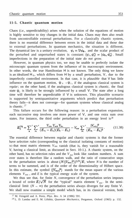
Chaotic quantum motion 353
11-5. Chaotic quantum motion
Chaos (i.e., unpredictability) arises when the solution of the equations of motionis highly sensitive to tiny changes in the initial data. Chaos may then also resultfrom uncontrollable external perturbations. For a classically chaotic system,there is no essential difference between errors in the initial data and those dueto external perturbations. In quantum mechanics, the situation is different.The dynamical law is a unitary evolution, and the scalar product ofthe perturbed and unperturbed states is constant: . Smallimperfections in the preparation of the initial state do not grow.
However, in quantum physics too, we may be unable to perfectly isolate themicroscopic quantum system from the influence of its macroscopic environment.In other words, the true Hamiltonian H is not known. The only thing we knowis an idealized H 0 , which differs from H by a small perturbation, V , due to theimperfectly controlled environment. In that case, it is plausible that V has littleinfluence on the quantum motion,regular; on the other hand, if the analogous classical system is chaotic, the finalstate ψ t is likely to be strongly influenced by a small V . The state after a longtime will therefore be unpredictable if V is unknown. This plausible scenariois supported by semiquantitative arguments which predict that perturbationtheory fails—it does not converge—for quantum systems whose classical analogis chaotic. 27
This failure occurs for the following reason: in a perturbation expansion,each successive step involves one more power of V , and one extra sum overstates. For instance, the third order perturbation in an energy level is 28
ψ o →ψ t , if the analogous classical system is
(11.38)
The essential difference between regular and chaotic systems is that the formerhave selection rules (corresponding to the classical isolating constants of motion)SO that most matrix elements Vmn vanish (that is, they vanish for a reasonableV, having a classical limit, as discussed in Sect. 10-1.). A chaotic system, on theother hand, has no selection rules and the V mn look like random numbers. A sumover states is therefore like a random walk, and the ratio of consecutive stepsin the perturbation series is about where N is the number ofterms to be summed, and is of the order of the dimensionality of Hilbert space.In this estimate, the symbol stands for the mean square of the variouselements V mn , and E is the typical energy scale of the system.
We thus see that, for finite N , convergence of the perturbation series imposesa bound of order for the “typical” matrix element V mn . In the semi-classical limit (N → ∞) the perturbation series always diverges for any finite V .We shall now examine a simple model which has, in its classical version, both
27 M. Feingold and A. Peres, Phys. Rev. A 34 (1986) 591.28 L. D. Landau and E. M. Lifshitz, Quantum Mechanics, Pergamon, Oxford (1965) p. 132.

354 Chaos and Irreversibility
regular and chaotic domains, and which is described, in its quantum version, bya finite-dimenssional Hilbert space, thereby avoiding the necessity of arbitrarytruncations.
Case study: twist and turn dynamics
The dynamical variables of this model are the three components of angularmomentum, J k . Their motion consists of a twist around the z -axis, given byEq. (10.4), followed by a 90° rotation around the y-axis. The total J is constant,and has a given value. The unitary evolution is therefore generated by
(11.39)
This system was extensively investigated by Haake, Ku and Scharf 2 9 who calledit a “kicked top.” (It is not really a top, because J z ², in the exponent, generatesa torsion, not a rigid rotation, of the corresponding classical system).
The classical analog of this unitary transformation is an area preserving mapof the unit sphere spanned by the vector J /J. We shall see that this “twistand turn” map has regular and chaotic domains, belonging to three distinctsymmetry classes (detailed numerical calculations will be presented for only oneof them). The purpose of this study is to find the effect of a change of the valueof the parameter α in Eq. (11.39), from 3.0 to 3.0003. These numerical valueswere chosen so that the model is near the limit of validity of perturbation theory.As intuitively expected, we shall see that quantum states localized in the regularregion of the classical phase space are impervious to this small perturbation.On the other hand, quantum states spread in the classically chaotic domain arestrongly affected by the small change in α .
Regular and chaotic domains of the unit sphere
Consider a sequence of mappings of the unit sphere x² + y ² + z ² = 1:
x' = z ,y' = x sin(αz ) + y C O S( α z ), (11.40)z ' = –x cos( αz) + y sin( α z),
The result of these mappings is displayed in the following figures, which weredrawn with an area preserving projection of the sphere onto the xz plane. Therelationship between radius R (on the paper) and r² := x² + z² = 1 – y² is
. Near the poles, R r (there is almost no distortion) and nearthe equator, R Equatorial area elements are stretched by a factorin the azimuthal direction (because ds = r dφ → Rd φ), and therefore they arecompressed by a factor in the radial direction.
29 F. Haake, M. Ku and R. Scharf, Z. Phys. B 65 (1987) 381.

355
Figure 11.6 shows a single orbit (10 5 points) generated by the twist and turnmap for α = 3.0. Most of the sphere is visited by that chaotic orbit, withthe exception of eight “forbidden” areas, which obviously correspond to regularregions of the map. These regular regions are located around fixed points oforder 1, 2 and 4, as shown in the following figures. Higher order fixed pointsalso exist, but the regular regions generated by them are barely visible and fartoo small to be significant.
Chaotic quantum motion
Fig. 11.6. A single orbit (105 points) covers most of theunit sphere, with the exception of eight regular regions.
There are two fixed points of order 1 (for a = 3.0) obtained by solving theequations x ' = x , y ' = y , z ' = z . These are
(11.41)
Orbits starting near these fixed points do not wander chaotically on the entiresphere. They are constrained to stay between invariant KAM lines, as shownin Fig. 11.7. Note that each fixed point can be obtained from the other one bya 180° rotation around the y-axis. This rotation will be denoted by Ry .
There is one fixed point of order 2, obtained by solving x '' = x , y '' = y ,z'' = z . It is
(11.42)
The result is shown in Fig. 11.8, together with nearby KAM lines. Note thata rotation of this fixed point around the x-axis by 180° (henceforth denoted byRx ) yields the pair of fixed points of order 1, together. This property, whichrelates two different types of motion, is called a dynamical symmetry.29

356 Chaos and Irreversibility
Finally, Fig. 11.9 shows the fixed point of order 4, at
(11.43)
The latter is obviously symmetric with respect to Ry and R x.Until now, we have considered individual orbits, that is, mapping of points
into points. A more general approach, giving new and instructive insights, isthe mapping of Liouville densities. Let us imagine that an infinitesimal “mass”ρ dA (which may be positive or negative) is attached to each area dA. Let usfurther assume that this mass is conserved by the twist and turn mapping, sothat its density obeys the linear law
Fig. 11.7. Two fixed points of order 1, surrounded
by KAM lines. (a) x 1 = z 1> 0 ; ( b ) x 1 = z 1 < 0.

Chaotic quantum motion 357
Fig. 11.8. Fixed point of order 2, surrounded by KAM lines.
ρ '(x', y' , z') = ρ (x, y, z), (11.44)
because dA' = d A. Note that, as the mapping (11.40) is continuous, nearbypoints are mapped into nearby points, so that a blob is always mapped intoa single blob (never into several disjoint blobs). In particular, the area foundbetween two nearby KAM lines is mapped onto itself. It follows that a Liouvillefunction for which ρ is constant between two closed KAM lines remains invariantunder any area conserving map. These invariant Liouville densities generalizethe fixed points which were discussed earlier.
Fig. 11.9. Fixed point of order 4.

358 Chaos and Irreversibility
In the model considered here, Liouville densities, whether invariant or not,may belong to three invariant symmetry classes of the twist and turn map,according to their behavior under Ry and R x (180° rotations around the y- andx-axes). For example, if ρ = F (x², y ², z², xyz ) is a single valued function of itsfour arguments, this ρ is even under R y and R x , and is mapped by Eq. (11.40)into another function of the same type. Likewise, any ρ = yF (x², y ², z ², xyz) iseven under Ry , odd under R x , and is mapped by (11.40) into a function of thesame type. For instance, the function ρ = y has this property, because
(11.45)
In summary, any ρ(x, y , z ) can be written as the sum of three terms, belongingto one the symmetry classes listed in Table 11-1. It will be no surprise thatquantum wave functions too can be classified according to the same symmetries.
Table 11-1. Symmetry classes of Liouville functions.
The quantum twist and turn map
Let us introduce dimensionless variables, so that
(11.46)
Here, j is an integer or half odd integer, and the jk are known numerical matricesof order 2j+1. It is convenient to choose a representation where jz is diagonal,with matrix elements m = j, . . . , –j, and eigenvectors denoted by |m⟩. Thenthe twist operator in (11.46) is diagonal too. The 90° rotation operator,
is explicitly given by30
3 0 E. P. Wigner, Group Theory, Academic Press, New York (1959) p. 167.
(11.47)

Chaotic quantum motion 359
The three symmetry classes which were discussed above at the classical levelnaturally appear again in the quantized version. First, consider R y = Q ². Itsmatrix elements, in the j z representation, are 30
(11.48)
It follows that Rx = Ry Rz has matrix elements . We shall henceforthrestrict our attention to even j. Suitable bases for the three symmetry classesare given in Table 11-2. The labels ee, oo and oe are reminders that the vectorsbelonging to the first class contains only even , and that they are even under
; and likewise for the other classes.
Table 11-2. Orthonormal bases for the three symmetry classes.
When written in this new basis, the U matrix (11.46) breaks down into a blockdiagonal form, with blocks of size j/2 + 1, j /2, and j . Each one of its threeinvariant subspaces is dynamically independent of the others. The numericalcalculations reported below were performed for the oo basis (R y even, R x odd)whose structure is the simplest. 31 There is no reason to expect that resultswould be qualitatively different in the other subspaces. These calculations wereperformed for j = 120, 500, and finally 1600. Intuitively, one expects quantummechanics to mimic classical mechanics for large j (at least, it ought to doso for a suitably restricted set of “reasonable” quantum states). Some of theproperties that were examined did not change much when j increased beyond120, but other ones necessitated the use of j = 1600.
Let us define two notions that will be useful for further discourse. The extentof a state is
(11.49)
Note that we must use | j z | , rather than simply j z , because for any statebelonging one of the symmetry classes. For a state ψ of the oo class, representedby j/2
(11.50)
31 A. Peres, in Quantum Chaos, ed. by H. A. Cerdeira, R. Ramaswamy, M. C. Gutzwiller,and G. Casati (World Scientific, Singapore, 1991) pp. 73–102.

360 Chaos and Irreversibility
an elementary calculation gives
(11.51)
where The extent of ψ is maximal ifand it is then equal to (j/2)–1. One could likewise define ∆| j x | and ∆ | j y | , butthe latter do not give any additional information on the eigenstates of U .
Another useful concept is the entropy of a state ψ with respect to a completeorthonormal basis eµ . This entropy is defined as follows. First, one computesthe relative weights of the basis vectors in the given state ψ :
(11.52)
The physical meaning of these p µ is that of probabilities. It is therefore naturalto call the expression
(11.53)
an “entropy.” The qualitative meaning of S is that e S is the number of basisvectors which are “appreciably involved” in the representation of ψ . The word“entropy” is appropriate in this context because S would indeed be the averagethermodynamic entropy released to the environment, if we performed maximalquantum tests for the basis e µ on an ensemble of quantum systems preparedin state ψ .
Perturbed map
Let us examine the response of our dynamical system to small perturbations.Assume that the original (unperturbed) system has twist parameter α = 3.0,and is described by a unitary matrix U satisfying
(11.54)
If we consider only states ψ in the oo symmetry class, the matrix U that hasto be used here actually is the oo block in the original unitary matrix given byEq. (11.46). I shall however use the same notation, U , for brevity.
The perturbed system differs from the original one by its twist parameter,α ' = 3.0003. It is described by a matrix U ', with
(11.55)
I have used different alphabets (Latin and Greek) to label the eigenphases φ m and φµ , and the corresponding eigenvectors vm and w µ , because there is noreason to expect a one-to-one correspondence between the eigenstates of U andthose of U ', unless the perturbation is sufficiently small. This is indeed thecrux of the problem. Such a one-to-one correspondence is the fundamental

Chaotic quantum motion 361
assumption of perturbation theory. In other words, the test for validity ofperturbation theory is whether each unperturbed vn has a low entropy w i t hrespect to the perturbed basis w µ.
These entropies,
(11.56)
are plot ted in Fig. 11.10 for the case j = 1600. It is seen that about 700eigenstates, out of the 800 in the oo subspace, have entropies of the order of 1(this value has no special significance), and therefore their eS is not close to 1,so that perturbation theory is not valid for these states. They are so sensitive tothe tiny change α → α' that they bear no resemblance at all to the eigenstatesof the pertubed U '. These states are called fragile.
On the other hand, we also see in Fig. 11.10 two “strings” of eigenstates ofU, having very low entropies. This means that each one of these states is nearlyidentical to one of the eigenstates of U '. States having that property are calledrobust. Upon closer examination, it is found that the string on the left of thefigure consists of a sequence of states with nearly equidistant eigenphases: thisis the Bohr quantization rule—the hallmark of eigenstates localized in a regularregion of the classical phase space. Indeed, the most localized (i.e., the leastextended) of these states have values of which are very close to thecoordinates of the fixed points of order 1 and 2, shown in Figs. 11.7 and 11.8.On the other hand, the second string of dots, whose extent is close to maximal,represents states localized near the fixed points of order 4.
To conclude this investigation, let us inquire how small the difference betweenα and α ' would have to be, to restore the validity of perturbation theory. Thecrude estimate given at the beginning of this section sets a limit of order N – 1/2
for the “typical” matrix element of the perturbing operator. This gives
(11.57)
The typical range of values for can be inferred from Eq. (11.49)and Fig. 11.10. That range is about the same as in the present case~ 0.1 j 2 . We thus obtain which indeed is the δαthat was used in this numerical example. (The parameters were chosen nearthe limit of validity of perturbation theory, in order to display both regular andchaotic types of motion, rather than fully developed chaos.) The correctnessof these estimates can also be directly seen in Fig. 11.10: even the most fragilestates there have only a moderate entropy. On the other hand, a totally chaoticsituation would effectively correspond to randomly chosen bases. In that case,it can be shown that the expected S would have been much larger, namely32
(11.58)
where γ = 0.5772 is Euler’s constant.
32 W. K. Wootters Found. Phys. 20 (1990) 1365.

362 Chaos and Irreversibility
Fig. 11.10. Sensitivity of eigenvectors of U to a perturbation, versus theirextent in | j z | space. The blob at the top contains extended and fragile states.The two strings contain robust states, localized near the classical fixed points.

Chaotic quantum motion 363
Robust and fragile states
Until now, we examined dynamical properties of the unitary mappings U a n d U' ,irrespective of the choice of a quantum state. The latter will be introduced next.Initially, it is an angular momentum coherent state (see page 329), satisfying
where n is a unit vector in the direction ( θ,φ). For such acoherent state, the uncertainty in jk is given by Eq. (10.141):
(11.59)
This means that the uncertainty in the direction of j is about j– 1 / 2k . More
precisely, the overlap of two distinct coherent states is given by Eq. (10.146):
(11.60)
where is the angle between the directions (θ´, φ') and (θ", ø "). For large j ,this overlap is about Two such states are almost orthogonal (in Hilbertspace) when In our case, with j = 1600, the angular resolution ofcoherent states is about 0.05 radian 3°. This is reasonably small, comparedto the size of a regular region on the unit sphere (see Fig. 11.7). This value of jis therefore sufficient to obtain a clean distinction between regular and chaoticquantum motions (smaller values of j would not be adequate).
Two cases will be considered. Their properties are summarized in Table 11-3.A “regular state” is obtained if the unit vector n points toward a fixed pointof order 1, as in Eq. (11.41). A “chaotic state” results from taking the samenx and n z as for but the opposite value of ny , so that the vector n willpoint into the midst of the chaotic region, as may be seen in Fig. 11.6.
Table 11-3. A tale of two states: the preparationand evolution of regular and chaotic vectors.
nx = n z of initial coherent state 0.6294126 0.6294126
ny of intial coherent state 0.4557187 –0.4557187
p 1 = highest weight 0.923359 0.021988
p2 = second highest weight 0.068007 0.015673
S (Entropy with respect to vn basis) 0.306937 5.66864
e s (Number of eigenvectors effectively involved) 1.35926 289.604
Average fragility of eigenvectors Σ p n S n 0.000116 1.140183
Average extent 22.1413 460.865
Time average of overlap — see Eq. (11.63) 0.857323 0.003923
Minimum overalp 0.716557 0 .0

364 Chaos and Irreversibility
We now project ψr and ψ c into the three invariant subspaces of U (defined inTable 11-2). Each projection must be considered independently of the others.This separation is essential, because symmetric regular regions, separated bychaotic ones, behave as a quantum mechanical double well (or multiple well) andthe eigenphases belonging to different symmetry classes form nearly degeneratemultiplets. A state initially localized in one of the regular regions will tunnel intothe other ones, and then, after some time, it will reassemble in the initial region,thus displaying a sequence of “collapses and revivals."29 ,33 This phenomenoncauses an unnecessary complication of the analysis. It does not appear if eachinvariant subspace is treated separately.
As before, we consider only the oo subspace. The projections of the initialstates ψr and ψc will be normalized to unity, and then simply called ψ r and ψ c ,
like the original states. First, we compute the statistical weightsand entropies S = We find radically different results for thetwo states: ψ r consists for the most part of a single eigenvector of U, while ψc
involves about 300 eigenvectors. Moreover, the eigenvectors used to build ψr
and ψ c have quite different properties, as may be seen from Fig. 11.11. Thechaotic state ψc is made of many fragile eigenvectors of U. On the other hand,the regular state ψr consists of a few robust eigenvectors.
The two eigenvectors which contribute most to ψ r will be called v 1 and v 2 .
Together, they make more than 99% of the initial state ψr . These robust eigen-vectors are in fact more stable than the corresponding eigenvalues! They areliterally pinned to the classical fixed points. Calling w 1 and w 2 the correspond-ing eigenstates of U ′, it is found that = 0.99993166. On the otherhand, the corresponding eigenphases φ1 and are well separated, by about0.0950 radian. (For comparison, the average separation between neighboringeigenphases of U is only 2π /800 = 0.0079 radian.)
Next, we turn our attention to the time evolution of ψ r and ψ c . Initially,when both are coherent states, their extent is given by = 21.9787.This can be compared with the extent of the most robust eigenstate, ψ r , w h i c his 19.11097. Then, as the vectors ψr and ψ c evolve, their extent will fluctuate
around a time average which is because interference termsbetween the various eigenstates vn do not contribute to that time average. Theresults are listed in Table 11-3. It is seen that ψ r retains its initial compactness,while ψ c spreads over most of the sphere.
Exercise 11.10 Derive the above expression for the time averaged extent.Hint: Use Eq. (11.51)
Regular and chaotic quantum motion
Finally, I come to the problem which motivated all this numerical work: thestability of the motion of ψ r and ψ c with respect to a small change of the twistparameter, from α = 3.0 to α '= 3.0003. A good indicator of the sensitivity
33 O. Bohigas, S. Tomsovic, and D. Ullmo, Phys. Rev. Lett. 64 (1990) 1479.

Chaotic quantum motion 365
Fig. 11.11. Sensitivity to perturbations vs relative weights pn of theeigenvectors of U which contribute most to the regular and chaoticstates ψ r and ψ c (shown by closed and open circles, respectively).

366 Chaos and Irreversibility
of the dynamical evolution to a small perturbation of α is the overlap of theperturbed and unperturbed state vectors. After t steps, a state which wasinitially ψ0 becomes
or (11.61)
where andThe scalar product of these two states is
(11.62)
Their overlap, Pt , is the absolute square of (11.62) and can be written as
oscillating terms. (11.63)
The first term on the right hand side of (11.63) is the time average of theoverlap. It is listed in Table 11-3, for ψ r and ψc , together with the minimumvalue of the overlap in the regular case. This minimum is obtained when thephase of the largest contribution to (11.62), namely is opposite tothe phase of all the other contributions. There is no minimum overlap in thechaotic case: the perturbed and unperturbed ψc can become orthogonal.
Figures 11.12 and 11.13 show the behavior of Pt over different time scales.The steady oscillations of the overlap of the two regular states are due to thefact that more than 99% of ψr is provided by two robust vectors, v1 and v 2, orw1 and w 2 . Their robustness (low entropy) implies thatwhile and are very small. Therefore Eq. [11.62] becomes
(11.64)
whence
(11.65)
In this case, perturbation theory converges and we have, from Eq. (11.35),
(11.66)
with a similar expression forOn the other hand, the overlap of the chaotic states and is
seen to decay very rapidly, and then to randomly fluctuate around an averagewhich is about l/N, where N = e S is the number of eigenstates which appre-ciably contribute to ψc . These fluctuations will effectively last forever, becauseEq. (11.63) involves N² 10 5 incommensurate frequency differences, and thetime needed for a Poincaré recurrence would be considerably larger than theduration of any conceivable numerical experiment.

Chaotic quantum motion 367
Fig. 11.12. The first 2000 steps. The overlap of the twochaotic states starts to decay quadratically with time,then as an exponential, and finally it fluctuates aroundits time average 0.003923 (shown by a broken line).
Exercise 11.11 Explain why the initial decay stages are quadratic.

368 Chaos and Irreversibility
Fig. 11.13. The first 200000 steps. Every hundredth step is shown. The brokenlines are the time averages of the overlaps, given by Eq. (11.63). The dottedline is the lowest value attainable by the overlap of the two regular states.
Exercise 11.12 Estimate how often there is a very low overlap of the twochaotic states (10 –10 , say ).

Evolution of pure states into mixtures 369
11-6. Evolution of pure states into mixtures
respective probabilities pα . The dynamical evolution then is
Exercise 11.13 Show that ρ ' in Eq. (11.67) satisfies
so that the entropy never decreases.
The quantum determinism postulate (page 237) asserts that a quantum systemprepared in a pure state remains pure when it evolves in a perfectly controlledenvironment. More generally, the entropy, S = , remains invariantunder the unitary evolution On the other hand, if the en-vironment is not perfectly controlled and is only statistically known, we mustreplace the evolution operator U by an ensemble of unitary matrices Uα , with
(11.67)
(11.68)
Another mechanism which leads to a similar result is the entanglement of aquantum system with other systems, found in the environment. In that case,if we use a formalism which ignores the systems belonging to the environment,the entropy also increases, by virtue of the subadditivity theorem (9.21).
The role of quantum chaos in irreversibility
In the preceding section, we saw that a small perturbation of the Hamiltonianmay cause, over a long time, large deviations from the unperturbed motion: theperturbed and unperturbed quantum states become nearly orthogonal. There-fore, if the perturbation is unknown, the final state is a mixture. All this wasshown for a fixed perturbation. Obviously, the situation can only be worse forrandom time-dependent pertubations (which are commonly called noise) .
It is now possible to reformulate, in the quantum language, the “ice cube inboiling water” paradigm that was proposed in Sect. 11-2. Consider again thetwist and turn map (11.46). The question is: can we prepare a quantum stateψ0 such that, after 105 steps, we obtain, to a good approximation, a prescribedcoherent state Figure 11.13 indicates that, in the presence of noise, theanswer critically depends on the type of state that we intend to reach.
Suppose, for example, that we want to obtain at the end of the evolution thestate ψr . The latter mostly consists of two robust eigenvectors. Therefore, evenif we cannot control the precise value of the twist parameter α, we still knowthat the motion is stable and that deviations from the planned evolution arebounded: Eqs. (11.65) and (11.66) show that the amplitude of the oscillationsis independent of δα (it is only their frequency which is proportional to δα) .
On the other hand, if we want to prepare a state that will become, after 105
steps, the coherent state ψ c , we must control the value of α with an accuracy

370 Chaos and Irreversibility
better than the limit given by Eq. (11.57). If we are unable to achieve suchan accuracy, we have every chance of landing far from our target—in a statewhich will be nearly orthogonal to ψ c. In that case, it is justified to say that theevolution which starts from the state ψc is irreversible : the reverse evolutioncannot be prepared.
11-7. Appendix: PostScript code for a map
The figures in this book, including the various maps in the present chapter, weredirectly generated by a P OST S CRIPT laser printer. P OST S CRIPT is a computerlanguage with powerful graphics capabilities.34 Although its primary applica-tion is graphics, P OST S CRIPT can also be used for ordinary computation, and itmay be quite convenient if a graphic output is desired. In particular, a few linesof code can easily generate an iterative map. The computation is entirely doneby the microprocessor in the laser printer itself. It could surely be done fasterby an ordinary computer, but then the bottleneck would be the transmission ofdata from the computer to the printer. How much time would your equipmentneed to transmit 10 6 coordinate pairs for drawing Fig. 11.2? If this is moretime than you can afford, use P OST S CRIPT. It is an efficient tool for generatingiterative maps.
As an example, here is the program which draws Fig. 11.3:
% !% Figure 11.3 (evolution of Liouville domain)300 400 translate%/Times-Italic findfont 12 scalefont setfont–9 73 moveto (p) show 72 –10 moveto (q) shownewpath –80 0 moveto 75 0 lineto
newpath –10 0 4 –30 30 arc 0 0 lineto closepath fill
0 –80 moveto 0 75 linetogsave 0 80 translate
newpath 0 –10 4 60 120 arc 0 0 lineto closepath fill
newpath –200 dup moveto 200 –200 lineto 200 dup lineto–200 200 lineto closepath stroke
COORDINATE SYSTEM
gsave 80 0 translate
grestore
grestore0.2 setlinewidth stroke
/Times-Roman findfont 12 scalefont setfont20 65 moveto (3 steps) show 84 –63 moveto (6 steps) show
34 Adobe Systems Inc., PostScript Language Reference Manual, Addison-Wesley, Reading(1985).

Bibliography 371
36000 /n n 1 add def/a n .01 mul def/p a sin r mul round cvi def/q –75000 a cos r mul add round cvi def2 3 /q q p add
dup 92681 gt 185362 sub ifdup –92681 It 185362 add if
def
200 92681 div dup scale%/r 10000 def200 setlinewidthnewpath –75000 0 r 0 360 arc stroke%/Helvetica findfont 250 scalefont setfont/n 0 def
A CIRCULAR DOMAIN
THE DYNAMICAL MAP
% every 1/100 of degree
/p q dup abs 92681 sub mul 92681 idiv p adddup 92681 gt 185362 sub ifdup –92681 It 185362 add if
def repeatq p moveto (.) show
repeat repeat
showpage
In order to accelerate the execution of this iterative map (which may takeseveral minutes, before the P OST S CRIPT printer outputs a page) the code waswritten with integer arithmetic, which is faster than floating point arithmetic,and more easily transportable to another computer. The variables q and p inthis program are not the original variables q and p, but are the integers closest to92681 q and 92681 p. The prime number 92681 is just less than 2 16.5 = 92681.9,so that the expression q (926811– q) is always less than 2 31 , which is theP OST SCRIPT limit for integers.
11-8. Bibliography
New York (1991).
F. Haake, Quantum Signatures of Chaos, Springer, Berlin (1992).
L. E. Reichl, The Transition to Chaos, Springer, New York (1992).
M. Tabor, Chaos and Integrability in Nonlinear Dynamics, Wiley, New York
M. C. Gutzwiller, Chaos in Classical and Quantum Mechanics, Springer,
(1989).
372 Chaos and Irreversibility
G. M. Zaslavsky, Chaos in Dynamic Systems, Harwood, Langhorne, PA(1985).
Some of these books also discuss dissipative chaos, which is fundamentally differentfrom the Hamiltonian chaos that was the subject of this chapter.
Recommended reading
An assortment of widely different approaches to quantum chaos can be found in thefollowing articles:
I. C. Percival, “Regular and irregular spectra,” J. Phys. B 6 (1973) L229.
M. V. Berry, N. L. Balazs, M. Tabor, and A. Voros, “Quantum maps,” Ann.Phys. (NY) 122 (1979) 26.
M. V. Berry, “Quantizing a classically ergodic system: Sinai’s billiard andthe KKR method,” Ann. Phys. (NY) 131 (1981) 163.
P. Pechukas, “Quantum chaos in the irregular spectrum,” Chem. Phys. Lett.86 (1982) 553.
M. C. Gutzwiller, “The quantization of a classically ergodic system,” PhysicaD 5 (1982) 183; “Stochastic behavior in quantum scattering,” ibid. 7 (1983)341.
M. Feingold, N. Moiseyev, and A. Peres, “Classical limit of quantum chaos,”Chem. Phys. Lett. 117 (1985) 344.
G. Casati, B. V. Chirikov, I. Guarneri, and D. L. Shepelyansky, “Dynamicalstability of quantum ‘chaotic’ motion in a hydrogen atom,” Phys. Rev. Lett. 56(1986) 2437.
J. Ford, G. Mantica, and G. H. Ristow, “The Arnol’d cat: Failure of thecorrespondence principle,” Physica D 50 (1991) 493.
G. P. Berman, E. N. Bulgakov, and G. M. Zaslavsky, “Quantum chaos ofatoms in a resonant cavity,” Chaos 2 (1992) 257.
R. Schack and C. M. Caves, “Hypersensitivity to perturbations in the quan-tum baker’s map,” Phys. Rev. Lett. 71 (1993) 525.
Experimental quantum chaos
J. E. Bayfield, G. Casati, I. Guarneri, and D. W. Sokol, “Localization ofclassically chaotic diffusion for hydrogen atoms in microwave fields,” Phys. Rev.Lett. 63 (1989) 364.
E. Doron, U. Smilansky, and A. Frenkel, “Experimental demonstration ofchaotic scattering of microwaves,” Phys. Rev. Lett. 65 (1990) 3072.
O. Agam, S. Fishman, and R. E. Prange, “Experimental realizations ofquantum chaos in dielectric waveguides,” Phys. Rev. A 45 (1992) 6773.

Chapter 12
The Measuring Process
12-1 . The ambivalent observer
Quantum phenomena do not occur in a Hilbert space. They occur in a labora-tory. Their description gives rise to the following dilemma: In order to observea physical system, we make it interact with an apparatus. The latter mustbe described by quantum mechanics, because there is no consistent dynamicalscheme in which a quantum system interacts with a classical one. On the otherhand, the result of the observation is recorded by the apparatus in a classicalform—perhaps it will be printed in a scientific journal. Therefore, a translationis needed from the Hilbert space formalism into a classical language.
The hallmark of a measuring instrument, which distinguishes it from otherphysical objects, is this ambivalence : it must be treated as a quantum systemwhile it interacts with the measured object, and as a classical system oncethe measurement is over. How can we “dequantize” the apparatus? Can this“dequantization” be done consistently?
Schrödinger’s cat
A vivid example of this ambivalence is Schrödinger’s legendary cat,¹ doomed tobe killed by an automatic device triggered by the decay of a radioactive atom.Initially, the combined state of the cat and the atom is L ⊗ u, namely a livingcat with an undecayed atom. After one half-life of the atom, this state becomes
(12.1)
with obvious notations. Nobody has ever seen a cat in such a strange situation.Clearly, the “cat paradox” arises because of the naive assumption that the
time evolution of the state vector ψ represents a physical process which is ac-tually happening in the real world. In fact, there is no evidence whatsoever
¹E. Schrödinger, Naturwiss. 23 (1935) 807 [transl. in Quantum Theory and Measurement,
ed. by J. A. Wheeler and W. H. Zurek, Princeton Univ. Press (1983) p. 1521.
373

374 The Measuring Process
that every physical system has at every instant a well defined state ψ (or adensity matrix ρ) and that the time dependence of ψ ( t ), or of ρ (t), representsthe actual evolution of a physical process. In a strict interpretation of quantumtheory, these mathematical symbols represent statistical information enablingus to compute the probabilities of occurence of specific events. For example,Eq. (12.1) tells us that if Schrödinger’s gedankenexperiment is repeated manytimes, about one half of the cats will be found alive and one half will not. Theinformation specified by ψ ( t ) , or ρ (t), can evolve because of known dynami-cal interactions (such as those causing the decay of the radioactive atom); itcan also get degraded, and ultimately obsolete, with the passage of time if theHamiltonian is incompletely known (especially if the system is chaotic, as wehave seen in the preceding chapter).
Some physicists are not satisfied by the above pragmatic attitude. Whilethey readily accept uncertainty relations, they would like to have at least adefinite ontology for quantum theory. There have been many attempts to savethe objectivity of the wave function by arguments such as: “Nobody has everseen a cat in state (12.1), but this is only because the mere observation of thecat causes ψ to jump² into either the L ⊗ u or the D ⊗ d state” (this jump iscalled a collapse³ of the wave function). There is nothing formally inconsistentin this scenario, but it is nevertheless incredible, as it implies a powerful andmysterious interaction between the brain of the observer and the entire body ofthe cat. A measurement, after all, is not a supernatural event. It is a physicalprocess, involving ordinary matter, and whatever happens ought to be analyzedby means of the ordinary physical laws.
Everett’s interpretation and other bizarre theories
Another attempt4 to salvage quantum ontology, without invoking a collapse ofthe wave function, is to assume that an entangled expression like (12.1) doesrepresent the actual situation. More precisely, the right hand side of (12.1) is apart of the “wave function of the Universe,” in which the cat may be consideredas the observer of the atom. However, the two branches of (12.1) correspondto different worlds, between which there can be no communication, once anirreversible process has occurred. This approach has several variations
5which
are called the “relative state interpretation” and the “many worlds interpreta-tion.” None is satisfactory because they merely replace the arbitrariness of thecollapse postulate by that of the no-communication hypothesis. In particular,there are no objective criteria for the occurrence of the irreversibility which isneeded to prevent communication between the various worlds (and there cannotbe any such criteria, as we have seen in Chapter 11).
²P. A. M. Dirac, The Principles of Quantum Mechanics, Oxford Univ. Press (1947), p. 36.³D. Bohm, Quantum Theory, Prentice-Hall, Englewood Cliffs (1951) p. 120.4H. Everett, III, Rev. Mod. Phys. 29 (1957) 454.
5M. A. B Whitaker, J. Phys. A 18 (1985) 253.

The ambivalent observer 3 7 5
There have also been innumerable attempts to modify quantum theory (notonly to reinterpret it) so as to avoid the dual nature of the measuring instrument.There is no experimental evidence to support any one of these mutations ofquantum theory—there is much evidence against them. I shall not furtherdiscuss these groundless speculations.
A simple measurement model
To prove that a piece of hardware is a valid measuring instrument, one mustproduce a dynamical model of its interaction with the physical object beingmeasured. This model should be formulated in quantum mechanical terms, butit must also be understandable in a semiclassical way. A simple example willillustrate how the same physical system may accept two conflicting descriptions,under different circumstances.
Consider again the Stern-Gerlach experiment which was discussed in a clas-sical way in Sect. l-5, but now use quantum mechanics instead. The dynamicalvariable which is measured is a component of the magnetic moment of an atom,µz say. The “pointer” indicating the observed value of µz is the center of mass rof that atom. Indeed, it is the final value of r that is irreversibly recorded by adetecting device. The dynamical description of the measuring process involvestwo stages. When the atom passes through the inhomogeneous field B of theStern-Gerlach magnet (see Fig. 1.5), its Hamiltonian,
(1.4)
includes an interaction between the magnetic moment µ, a component ofwhich is the “measured system,” and the center of mass r which plays therole of the “measuring system.” The atom thus embodies both systems.(The symbols r and p denote classical variables or operators, according tothe context.) The equation of motion for p, the variable conjugate to r, i s
, just as in Eq. (1.6), but with [p, H ]P B replaced bya commutator since we are now discussing quantum systems.
However, once the atom leaves the magnet, its Hamiltonian H = p ²/2m n olonger couples µ and r. The equations of motion have the same solution,
(12.2)
in classical and in quantum mechanics. If you prefer, the equation of motionfor the quantum Wigner function, Eq. (10.67), is identical to that for a classicalLiouville density. Nothing irreversible has occurred as yet at this stage, at leastin principle.6 In particular, the first stage of amplification —a necessary stepfor a quantum measurement-is simply due here to the passage of time, whichcan make the factor t/m in Eq. (12.2) arbitrarily large.
6 J. Schwinger, M. O. Scully and B.-G. Englert, Z. Phys. D 10 (1988) 135.

376 The Measuring Process
The consistency problem
It must now be shown that no inconsistency arises if the measuring instrument,or the “observer” (in the above example, the center of mass position r), is con-sidered as a genuine quantum object for which no classical description is used,but this quantized instrument is, in turn, observed by some other instrument,having both quantum and classical descriptions. For example, it should notmatter whether Schrödinger’s cat is considered as the observer, or is an intrin-sic part of the atom-cat dynamical system which is observed by someone else.The reason for suspecting a possible inconsistency is the following:
If the observer were not a cat or some other, possibly inanimate but utterlycomplicated measuring apparatus, the unitary evolution leading to Eq. (12.1)would be reversible. Simple, highly idealized models of measuring apparatusescan easily be concocted, which have that property.7 After the measurementis achieved (i. e., the instrument is correlated with the measured system), itstill is possible to undo the whole process: A superobserver, capable of fullyanalyzing the dynamical behavior of the measuring apparatus (e. g., capable ofwriting explicitly the Hamiltonian of Schrödinger’s cat) could cause the originalobserver (or apparatus —this makes no difference) to decorrelate itself from themeasured system and to “unlearn” the result of the measurement. For example,the cat would be resurrected. And then, the superobserver, by measuring againthe same system, could obtain a different result for his measurement.
If such a scenario were indeed possible, the notion of measurement wouldbecome meaningless, as no measurement would ever be conclusive. Consistencythus requires the measuring process to be irreversible. There are no super-observers in our physical world.
Formally, the logical consistency of the “dequantization” of a measuringapparatus implies the equivalence of two different descriptions of the same pro-cess, in which a quantum system S is coupled to an apparatus A, as in Eq. (1.4)above. Let this composite system evolve in time, and then trace out S in itscombined density matrix, so as to obtain a reduced ρA for the apparatus. Thisreduced density matrix can be converted by means of Eq. (10.56) into a Wignerfunction, WA (q, p). Some blurring (see page 316) converts the latter into afuzzy Wigner function which is nowhere negative and may be interpreted as aLiouville density ƒA (q , p), if the terms in the quantum Liouville equation(10.67) are negligible for the macroscopic apparatus. Notice that we obtain aprobability distribution for the final state of the apparatus. We cannot demanda definite result, since quantum theory makes only statistical predictions.
Consider now a second, bigger apparatus, B, which interacts with apparatusA, in order to measure it. This is a classical measurement. We have a com-bined Liouville density for A and B. After it evolves according to the Liouvilleequation, we sum over the variables of A and get a reduced Liouville densityF B (Q , P) for the big apparatus. All this is quite simple and straightforward.
7 A. Peres, Am. J. Phys. 42 (1974) 886.

The ambivalent observer 377
We can however follow an alternative approach, and this possibility givesrise to a consistency problem. Instead of dequantizing ρA to obtain ƒA ( q , p ),we can describe both apparatuses by quantum mechanics, let the compositequantum system evolve unitarily, and then trace out A to obtain a reduceddensity matrix ρB . The latter is converted into a Wigner function WB (Q, P)which, after some blurring, yields a new Liouville function FB (Q, P).
The consistency issue is obvious: Is FB (Q, P) the same as FB (Q, P) whichwas obtained by the preceding method? This is quite unlikely, in view of themany arbitrary steps in the above calculations. However, since we are onlycalculating probabilities—because quantum theory predicts nothing else—smalldiscrepancies between these two Liouville densities should not be a matter ofconcern. It is this (approximate) objectivity which characterizes a properlyexecuted measurement (i.e., a quantum test). The result is definite and cannotbe affected by reconsidering the measuring apparatus as a quantum object, tobe observed by still another apparatus. If the latter is reasonable, it will giveresults which almost always agree with those of the first apparatus.
The last two clauses must be noted. The restriction to reasonable apparatuses(that is, those measuring only reasonable operators, as defined at the beginningof Chapter 10) is equivalent to the former statement that “there are no super-observers.” The proviso almost always is essential. It gives a fuzzy aura to thenotion of quantum measurement, but there is no escape from this fuzziness.There can be no unambiguous algorithm for converting the quantum languageinto an utterly different classical language.
A classical description is not an approximation of a quantum description,but is qualitatively different .
8A classical pointer has a position which is a real
number. A quantum pointer also has a position, but the latter is an opera-tor. There are questions, such as “what is the numerical value of the pointerposition,” which make sense in the classical language, but are meaningless inthe quantum language. The only vestige of quantum theory which a classicaldescription may retain is the canonical uncertainty relation, namely a minimumspread of order in the 2n-dimensional phase space.
Open systems
When is a physical system a good measuring instrument, satisfying the aboveconsistency criteria? An obvious necessary condition is that it is not isolatedfrom the environment where the outcome of the test is recorded in a durablestructure. Therefore irreversibility is a necessary feature of quantum tests. Asimple model will illustrate these points.
Le t be the initial state of a quantum system which is submittedto a maximal test corresponding to the orthonormal basis um . The measuringapparatus has an initial state φ (there is no harm in assuming that this is a purestate, see Exercise 5.10). Let vn α set of final states of that apparatus. The
8 A. Peres and W. H. Zurek, Am. J. Phys. 50 (1982) 807.

378 The Measuring Process
index n refers to a macroscopic degree of freedom, such as the position of thecenter of mass of a pointer which indicates which one of the states un has beenfound in the test. The index α refers to additional, microscopic, “irrelevant”degrees of freedom, such as the internal energy levels of the pointer. Thereforethe orthonormal states vm α and v n β are macroscopically distinguishable only ifm ≠ n. With these notations, the result of the interaction of the apparatuswith the system under study is assumed to be:
(12.3)
This is a linear superposition—it cannot be anything else, if quantum theory iscorrect. For example, Eq. (12.1) is such a superposition. The process (12.3) iscalled a “measurement,” because the nth state of the system is correlated withthe n th set of macroscopically distinguishable final states of the instrument.
Here, it should be pointed out that Eq. (12.3) does not represent the mostgeneral type of measurement process. The latter corresponds to a positiveoperator valued measure (POVM) as explained in Sections 9-5 and 9-6. Thepresent discussion is restricted, for simplicity, to repeatable tests, also called“von Neumann measurements,” or “measurements of the first kind.” The fun-damental issue of irreversibility is the same for all these processes.
Exercise 12.1 Show that the evolution (12.3) is unitary, provided that
and construct a Hamiltonian which generates this evolution.
(12.4)
If we now want to reverse the arrow in Eq. (12.3), so as to decorrelate theobserved system from the observer, we must specify not only a few coefficients cncorresponding to macroscopically distinguishable states, but every single micro-scopic cn α , with the correct amplitude and phase. Here lies the difficulty. Thedynamics of the internal degrees of freedom of any macroscopic apparatus isinherently chaotic. Therefore the values of the cnα are highly sensitive to anyinteractions with an uncontrollable external environment, weakly coupled to thedegrees of freedom of the apparatus.9 Reversing the unitary evolution (12.3),for example resurrecting Schrödinger’s cat, is an impossible task.
12-2. Classical measurement theory
Uncertainty relations exist in classical mechanics, just as in quantum mechanics.As there must be an interaction between the apparatus and the observed system,measuring one property of the system necessarily causes a disturbance to some
9 A.Peres, Phys. Rev. D 22 (1980) 879.

Classical measurement theory 379
of its other properties. In particular, any uncertainty in the preparation of themeasuring apparatus affects the subsequent dynamics of the measured system,after completion of the measurement.
To give a concrete example, consider a classical system with HamiltonianH0 (q, p) and suppose that we want to measure one of its dynamical variables,A(q, p), at time t0 . An ideal measurement is performed as follows. We couplethe system to an apparatus which, in the present extreme idealization, simplyis a free particle (a “pointer”) of mass M, position Q, and momentum P. Thecomplete Hamiltonian is
(12.5)
where g(t – t 0 ), the strength of the coupling, is controlled by other degrees offreedom (not included in H) in such a way that g (t – t 0 ) is very large whent 0 < t < t 0 + ∈ , and negligible for other t. For example, in a Stern-Gerlachexperiment, t0 is the time of entrance into the magnet, and t0 + ∈ is the exittime.9 These two parameters are determined by the translational motion of theatom.
We shall now assume that the interaction term in (12.5) dominates all theother terms—which can therefore be neglected—during the brief duration ofthe measurement. Let us define, for further use,
(12.6)
The equations of motion of the “pointer” are:
(12.7)
and
(12.8)
Likewise, for any variable B(q, p) of the apparatus, we have
(12.9)
From (12.7) it follows that P is a constant: P = P 0 . In the special case whereB = A, Eq. (12.9) gives which is a finite quantity. Therefore, thechange in A during the very brief interaction is of order ε and can be neglected.We thus obtain, from (12.6) and (12.8),
(12.10)
which gives us the value of A (t0 ), that we wanted to know. Assuming forsimplicity that Q (t0 + ε) is measured with perfect precision, the uncertainty inthe recorded value of A(t0 ) is
380 The Measuring Process
(12.11)
where ∆Q0 is the uncertainty in the initial position of the “pointer.”Consider now any other variable B. We have, by integration of (12.9),
(12.12)
which involves the time average of the Poisson bracket during the measurement.If the initial value P0 is known with a precision ∆P0 , the final value B (t 0 + ε )will be uncertain by
(12.13)
It follows that
(12.14)
This result looks like the quantum uncertainty relation (4.40). However, theabove argument was purely classical. The only role quantum theory could havein this issue is to set an absolute lower bound to the value of ∆Q0 ∆ P0 , irre-spective of the experimenter’s skill. We thus see why elementary semiclassicalarguments, such as the one commonly presented for Heisenberg’s microscope,end up with the same quantum uncertainty as the full quantum treatment. Thisis simply due to the similarity of Poisson brackets and commutators, which holdsfor reasonable dynamical variables (as defined in Sect. 10-1).
Consecutive measurements
Suppose now that we want to know not only the value of A at a given time t0 ,but the complete time evolution A (t), or at least a sequence of values A(t j ) .Obviously, if the value of A (t 1 ) depends, via the equations of motion, on thevalue of B (t0 ), and if [B, A]P B ≠ 0, then A t( 1 ) will be affected by the disturbanceto caused by a prior measurement of A (t0 ).
This can also be seen as follows: It is always possible, in principle, to expressas a function of q (t0 and p (t 0) with arbitrary accuracy (this can be done)
analytically, in closed form, if the equations of motion are integrable, but even ifthey are not, perturbative methods are readily available). We may thus defineunequal time Poisson brackets . From the preceding argument,it follows that the measurement of A(t ) does not perturb if, and only if,
(12.15)
When this condition is satisfied by a dynamical variable, it is possible to monitorits evolution in a noninvasive way, that is, without affecting that evolution.Dynamical variables which satisfy Eq. (12.15) will be called robust. (In quantumtheory, they are called QND-variables for “quantum nondemolition.")
A simple example of a variable which is not robust is the position x of a freeparticle. Since we obtain
B (t0 )
A (t 1 )
A (t 1 )0

Classical measurement theory 381
(12.16)
A more complicated example is discussed below.
Case study: a forced harmonic oscillator
A situation where classical and quantum physics come in close contact is thedetection of gravitational radiation. A gravitational wave is a time-dependentinhomogeneity of the gravitational field, caused by the violent motion of distantmasses, and propagating at the speed of light. It acts as a tidal force whichproduces oscillations in the distance between neighboring particles. The lattermay be free to move (for example, they may be the mirrors of an interferometricdetector) or they may be part of a massive “antenna” in which a dynamic strainis induced. 10,11
The problem of detecting gravitational waves may seem completely divorcedfrom quantum theory. Fields are weak, frequencies are low, and the effects ofquantized gravity are totally negligible. All we want to measure is a classicalsignal ƒ(t) a component of the Riemann tensor, averaged over the size ofthe detector. There should be no quantum uncertainties, and no lower limitto the detectable ƒ(t). The difficulty is solely due to the fact that gravitycouples very poorly to the dynamical variables of any detector. This has thefollowing consequence, if we use classical mechanics to perform calculations. Thedynamical variables follow an orbit in the classical phase space. The unknownvalue of the signal, ƒ(t), has ot be calculated from the properties of that orbit.However, if the signal is very weak, the orbit may encompass a domain smallerthan . This means, effectively, that classical mechanics is not applicable andthe detector must be treated as a quantum system. New problems then arise,which will be discussed in Sect. 12-4.
Let us first consider the properties of a classical forced harmonic oscillator.It is assumed that the noise temperature is low enough to allow us to neglectnoise and other dissipative effects. With suitable units of mass and time, theHamiltonian is
(12.17)
The driving force ƒ(t ) is unknown and the problem is to deduce its value frommeasurements of x and p. The equations of motion are
and (12.18)
These equations can be integrated as follows. Define new variables
A := x cos t – p sin t and B := x sin t + p cos t. (12.19)
10 J. Weber, Phys. Rev. 117 (1960) 306.11 P. F. Michelson, J. C. Price, and R. C. Taber, Science 237 (1987) 150.

382 The Measuring Process
We obtain
and (12.20)
whence
(12.21)
and
(12.22)
The last equations define functions C (t) and S (t) which have to be determinedexperimentally. We have, from (12.19),
(12.23)
It follows that and so that neitherx nor p is a robust variable, satisfying (12.15).
Exercise 12.2 Show that the oscillator energy is also notrobust, because it satisfies
If we are interested in a continual monitoring of f(t), it would therefore bea bad idea to measure x, or p, or E. On the other hand, the variables A ( t )and B (t ) are manifestly robust see Eqs. (12.21) and (12.22) and one of them(but not both!) can be continually monitored. For example, we may chooseto measure repeatedly A(t) at the cost of perturbing in an unknown way thevalue of B (t), or vice versa. By continually monitoring A(t), we obtain thefunction S(t) from which we can retrieve the value of f( t). This method iscalled “homodyne” (or “phase-sensitive”) detection.
The next problem is to materialize the symbols cos t and sin t whichappear in Eq. (12.19). Their values are generated by a clock. A clock is notan abstract notion. It is a physical system, with dynamical degrees of freedomwhich must be represented in terms of canonical variables and introduced in theHamiltonian. Conceptually, the simplest clock is a rotor described by an angleθ and its conjugate momentum J, with Poisson brackets [θ , J] = 1. The newP BHamiltonian, including that clock, may be taken as
(12.24)
It gives the same equations as before, together with = 1 and = 0. Theseadditional equations of motion have solutions θ = θ0 + t and J = const. Wenow define, instead of (12.19),

Classical measurement theory 383
A = x cos θ – p sin θ and B = x s i n θ + p cos θ, (12.25)
and we obtain
and (12.26)
with solution
(12.27)
This gives, with the same notations as before,
(12.28)
Note that A (t) and B (t) are robust, because the integrals on the right handsides of (12.27) have vanishing Poisson brackets with A0 and B0 .
The difficulty is that there is no known way of materializing this rotor clock.In quantum theory, it would give a Hamiltonian whose eigenvalues have no lowerbound, which is unacceptable. (An approximate construction was proposed byUnruh. 12 ) It is also possible to construct, as shown in Sect. 12-7, a rotor clockwith a finite number of quantum states, but in the finite Hilbert space of thelatter neither cos θ nor sin θ (let alone θ itself) are well defined operators.
A more practical alternative is an oscillator clock, with the same frequencyas the original oscillator. For example, this clock could be an electric LC circuit,coupled to the mechanical oscillator by a suitable transducer.13 Let y and p y
be the dynamical variables of the second oscillator. The Hamiltonian becomes
(12.29)
where px now stands for the former p. The equations of motion are the sameas before, together with and which are easily solved. Define
and (12.30)
and also (for later use)
(12.31)
These dynamical variables have Poisson brackets
12 W. G . Unruh, Phys. Rev. D 19 (1979) 2888.13 C .M. Caves, K. S. Thorne, R. W. P. Drever, V. D. Sandberg, and M. Zimmermann, Rev.
Mod. Phys. 52 (1980) 341.

384 The Measuring Process
[A, B ]PB = 2D , [B , D] PB = 2A , [D, A] PB = 2B , (12.32)
like components of angular momentum (multiplied by 2). This property hasimportant consequences when quantization is considered: the observable valuesof A (or B, or D) are integers, and therefore cannot evolve continuously as inclassical mechanics. Intuitively, the probability of a jump from one eigenvalueto another depends on the lapse of time between consecutive measurements. Adetailed calculation, given in Sect. 12-5 below, shows that if measurements arevery frequent on the natural time scale of the observed system, that systemappears to be paralyzed: the value of A never changes. This is called thequantum Zeno effect. To avoid it, one must make fuzzy measurements, whichdo not discriminate between consecutive eigenvalues, and do not prevent theevolution of the system.
Let us return to the classical equations of motion of our driven harmonicoscillator. With the use of an oscillator clock, we have
and (12.33)
Therefore and It follows that neither A nor B i srobust. We have already seen in Exercise 12.2 that D is not.
We can solve (12.33) explicitly:
(12.34)
whence, with the help of
(12.35)
There are similar expressions for B(t). Comparison with Eq. (12.28) shows theessential difference between rotor and oscillator clocks. The variables sin θ andcos θ have a vanishing Poisson bracket. On the other hand, the oscillator clockvariables satisfy [y0, py0 ]PB = 1, which givesTherefore the measurement of A 0 causes an unknown disturbance to the valueof A( t ). We have
(12.36)
where Q and P are the dynamical variables of the apparatus that measures A.Usually, ∆Q ∆ P is much larger than its quantum limit /2.
The important result here is that the right hand side of (12.36) is independentof the clock variables y and py ,while A (t ) itself is proportional to the amplitudeof the clock oscillations. As the latter can in principle be made as large as wewish, irrespective of the weakness of the signal f( t ), the uncertainty in A (t ) canbe made negligibly small, when compared to A( t) itself. The clock essentially serves to amplify the weak signal f (t ), and it is theoretically possible to measuref (t ) with arbitrary accuracy. The only problem is to realize in the laboratorythe couplings that were written in the above equations.
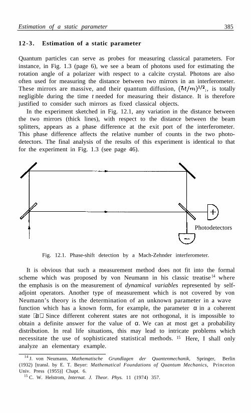
Estimation of a static parameter 385
12-3 . Estimation of a static parameter
Quantum particles can serve as probes for measuring classical parameters. Forinstance, in Fig. 1.3 (page 6), we see a beam of photons used for estimating therotation angle of a polarizer with respect to a calcite crystal. Photons are alsooften used for measuring the distance between two mirrors in an interferometer.These mirrors are massive, and their quantum diffusion, , is totallynegligible during the time t needed for measuring their distance. It is thereforejustified to consider such mirrors as fixed classical objects.
In the experiment sketched in Fig. 12.1, any variation in the distance betweenthe two mirrors (thick lines), with respect to the distance between the beamsplitters, appears as a phase difference at the exit port of the interferometer.This phase difference affects the relative number of counts in the two photo-detectors. The final analysis of the results of this experiment is identical to thatfor the experiment in Fig. 1.3 (see page 46).
Photodetectors
Fig. 12.1. Phase-shift detection by a Mach-Zehnder interferometer.
It is obvious that such a measurement method does not fit into the formalscheme which was proposed by von Neumann in his classic treatise 14 wherethe emphasis is on the measurement of dynamical variables represented by self-adjoint operators. Another type of measurement which is not covered by vonNeumann’s theory is the determination of an unknown parameter in a wavefunction which has a known form, for example, the parameter α in a coherentstate α⟩. Since different coherent states are not orthogonal, it is impossible toobtain a definite answer for the value of α. We can at most get a probabilitydistribution. In real life situations, this may lead to intricate problems whichnecessitate the use of sophisticated statistical methods. 15
analyze an elementary example.Here, I shall only
14 J. von Neumann, Mathematische Grundlagen der Quantenmechanik, Springer, Berlin(1932) [transl. by E. T. Beyer: Mathematical Foundations of Quantum Mechanics, PrincetonUniv. Press (1955)] Chapt. 6.
15 C. W. Helstrom, Internat. J. Theor. Phys. 11 (1974) 357.

386 The Measuring Process
Determination of polarization parameters
You are given a spin j particle, prepared in an angular momentum coherent state, and you are requested to evaluate the angles θ and φ. These are classical
parameters, whose value is determined by the orientation of the macroscopicapparatus which produced the spin j particle.
It is plausible that the best measurement method involves a non-orthogonalPOVM, as in Eq. (9.81), because θ and φ may take continuous values, while amaximal test (a von Neumann type measurement) has only (2j + 1) differentoutcomes. In the present case, the natural POVM to use is the one definedin Eq. (10.144): We divide the unit sphere into small areas sin θd θdφ, and foreach one of them we define a positive operator
(12.37)
These operators satisfy = , so that they indeed form a POVM.The probability of obtaining a particular as the result of the test is, by
virtue of Eq. (9.79), Using Eq. (10.146), we obtain
(12.38)
where Θ is the angle between the directions (θ,φ) and (θ' , φ ') .Once the test has been performed and has indicated a direction we
can derive the a posteriori probability distribution for the actual preparationdirection . If the a priori probability distribution was isotropic, namelysin the a posteriori probability can be found by Bayesian analysis(Sect. 2-77). The result is
Exercise 12.3 Verify that
Exercise 12.4 For the special case j = 12 , compare the above result with the
one in Eq. (9.11:0), which corresponds to a direct von Neumann measurement,rather than a POVM. Ans.: In this particular case, the information gain isthe same with both methods. This is no longer true for higher j.
Physical constants
Another common type of measurement is that of a physical constant, such asthe mass of an elementary particle or the magnitude of its magnetic moment.These unknown constants are c-numbers, and are measured in the same way asany other classical parameter. We perform quantum tests on particles whichhave been prepared in a known way. These tests are described by an interac-tion Hamiltonian where the unknown physical constants appear as numericalp a r a m e t e r s—for example m and µ in the Hamiltonian (1.4). We then attributeto these parameters the values which best fit the experimental results.

Time-dependent signals 387
12-4. Time-dependent signals
We now turn our attention to a more difficult problem, which is the detectionof weak classical signals. This is done by coupling the signal to a detector(a dynamical system of known structure) so that the Hamiltonian H of thedetector contains a term depending on the unknown signal. Then, by observingthe time dependence of a dynamical variable of the detector, we can reconstructthe entire H , including the unknown signal. An example of signal detection bysuch a method was discussed in Sect. 12-2, at the classical level.
When the signal is extremely weak, the quantum properties of the detectorcannot be ignored. There appears then to be a conflict between the continuousnature of a classical signal and the discrete spectrum of a quantum device.Moreover, the final result cannot be recorded by a quantum system, which maybe in a superposition of eigenstates. The detector has to be “measured” by asuitable apparatus (the “meter”) which then yields another classical signal—namely a sequence of real numbers. We shall now examine the distortion causedby the presence of a quantum interface between these two classical signals. Itwill be seen that a good meter should have a moderate resolution, so as to lumptogether numerous levels of the quantum detector. Obviously, a poor resolutiongives inaccurate results, but a resolution which is too sharp is also undesirable,because it impairs the correspondence between the input and output signals;and a perfect resolution, down to isolated eigenvalues, may completely lock thedetection process.
Fuzzy measurements
As a concrete example, let us return to the simplified version of the Stern-Gerlach experiment that was discussed at the beginning of this chapter, both inthe classical language and in the Heisenberg picture (formally, these two werethe same). I shall now use the Schrödinger picture, which is more appropriatein a situation where the Hamiltonian is not known and has to be determinedby observations. Further simplifications help to get a tractable problem. Weshall consider a particle of spin
21 whose initial state is described by a spinor
There are no other degrees of freedom and, at this stage, no forces acting onthat particle. The problem is to measure σz , a dynamical variable purportedto have observable values ±1.
The “meter” which performs this measurement is idealized as having a single,dimensionless degree of freedom, q, which indicates the value of the measuredvariable. The conjugate degree of freedom, p, satisfies [q,p] = i . A strippeddown Hamiltonian which describes the measuring process is
where g( t ) has a narrow support near t = 0, and satisfies
(12.39)

388 The Measuring Process
Let φ(q) denote the initial wave function of the meter. The time evolutiongenerated by the Hamiltonian (12.39) is
(12.40)
This process is illustrated by Fig. 12.2, where it was assumed that φ(q) has asharp maximum at q = 0, so that, before the measurement, it is most probableto find the meter near q = 0. The meaning of the right hand side of (12.40)is the following: There is a probability amplitude αφ(q – 1) for finding themeter near q = 1, and the particle with spin up; and a probability amplitudeβφ(q + 1) for finding the meter near q = –1, and the particle with spin down.
Fig. 12.2. Graphical representation of Eq. (12.40). In this drawing and the fol-lowing one, α = 0.8 and β = 0.6. The thick arrows indicate the spin orientation.
What we call “the observed value of σz” is the final position of the meter.The state vector (12.40) specifies the probabilities of observing the meter at itspossible final positions. Ideally, φ should have zero width and the result of themeasurement should be ±1, i.e., one of the eigenvalues of σ z . However, theactually observed value of σ z may differ from the ideal result by a quantity oforder ∆q, namely the width of the meter wave function. This discrepancy isnot a trivial “technical difficulty,” but a matter of principle. We shall actuallysee that in some cases it may be advantageous to make ∆q larger than theseparation of consecutive eigenvalues.
The situation when ∆q is broad is represented by Fig. 12.3. The probabilityof observing the meter between q0 and q 0 + dq 0 is
(12.41)
If the observed value q0 is such that both terms on the right hand side of (12.41)contribute, the final state of the spin 1
2 particle is not an eigenstate of σz . It isgiven by the right hand side of Eq. (12.40), evaluated at q = q0 , and properlynormalized.
For future reference, let us rewrite the preceding equations in terms of densitymatrices, for the measurement of an arbitrary operator A, with eigenvalues λm
(in the simple case considered above, A was σz and we had λ m = ±l). Let ρmn

Time-dependent signals
be the density matrix of the quantum system, in a representation where A isdiagonal. Let be the initial density matrix of the meter.The combined density matrix is
(12.42)
The Hamiltonian (12.39) becomes g(t )Ap and, instead of (12.40), we nowhave
(12.43)
This expression contains all the information about the correlated state of thequantum system and of the meter which was used for observing that system.
Fig. 12.3. This is the same as the final state in Fig. 12.2, exceptthat the initial location of the meter is uncertain by more than theseparation of the eigenvalues ±1, so that the measurement is “fuzzy.”
At this point, if we are no longer interested in the quantum system, wemay trace out the indices referring to it, and get a reduced density matrixfor the meter. Then, the average value of any observable function f(q ) — a f t e rcompletion of the interaction between the meter and the quantum system—is
(12.44)
where w j = ρ j j is the probability of occurence of the jth eigenstate of A , justbefore (and also after) the interaction. For example, if the meter is prepared ina symmetric state, φ(q) = φ ( –q ), we have
(12.45)
and
(12.46)
It follows that
(12.47)
where
389

390 The Measuring Process
(12.48)
and
(12.49)
are the variances associated with the states of the quantum system and themeter, respectively.
Conversely, if we are interested in the quantum system (for later use) butnot in the meter itself, the reduced density matrix ρ' mn of the quantum systemis obtained by tracing out q' and q" :
(12.50)
where S mn is the coherence matrix:16
(12.51)
Exercise 12.5 Show that S m n
E.g., if the meter is prepared in a coherent state,w e h a v e ∆ q = σ and
(12.52)
Obviously, S mm ≡ 1 (for any φ) so that the diagonal matrix elements ρ mm arenot affected by the measuring process. On the other hand, the off-diagonalelements of ρ are depressed by a factor Smn , and may even be reduced to zero ifthe displaced wave packets are mutually orthogonal, as in Fig. 12.2. However, if
as in Fig. 12.3, the off-diagonal elements of ρ are not completelysuppressed. In particular, if some eigenvalues are degenerate, the submatrix ofρ mn corresponding to these eigenvalues is not affected at all.
Consecutive measurements
The analysis of a time-dependent signal necessitates numerous consecutivemeasurements so as to get a sequence of numbers, corresponding to times17
t 1 , t 2 , . . . , and so on. Note that there can be no continuous measurement, if ameasurement is defined as a brief and intense interaction between the meterand the measured system, as in Eq. (12.39) f or example. In particular, the timedifference t k – t must be larger than the duration of g (t), so that consecutivek –1
measurements do not overlap.
16 A. Peres Phys. Rev. D 39 (1989) 2943.17 C. M. Caves, Phys. Rev. D 33 (1986) 1643; 35 (1987) 1815.

Time-dependent signals 391
natural time scale of the measured system. Such a measurement yields only
observed variable, as we shall see in Sect. 12-6. One can even consider a passivedetector, for example, a Geiger counter waiting for the decay of a nucleus. Sucha setup does not correspond at all to the present definition of a measurement.It is best described as a metastable system with several decay channels. 18
On the other hand, we may also consider measurements of finite duration,where the function g (t) is spread over an appreciable time, compared to the
a single number which corresponds, in the best case, to a time-average of the
Quantum theory does not impose any fundamental limitations to monitoringarbitrarily weak signals within arbitrarily short time intervals. Limitationsarise solely because we want to use—or are forced to use—some particulardetectors. For example, since gravitational radiation couples very weakly tomatter, detectors must be massive antennas11 or gigantic interferometers.19 I tis therefore impractical to have a large number of identical gravitational wavedetectors for the purpose of estimating quantum averages. We must extract asmuch information as possible from each measurement. In general, we would likethe quantum evolution to mimic the classical one, and the output signal to bean amplified replica of the input. Signal distortion should be minimized. Letus examine how well these aims can be achieved.
Consider a sequence of measurements performed at times t1 , . . . , t N , bymeans of meters with coordinates q 1, . . . , q N , respectively. The initial densitymatrix of the detector and the meters is a generalization of (12.42):
The Hamiltonian of the composite system is
(12.53)
(12.54)
a known functional dependence on the unknown signal. As before, there are noterms like p j 2 /2m j in the Hamiltonian: the masses of the meters are assumedso large that we can ignore the spontaneous spreading of each meter’s wavepacket.
with notations similar to those in Eq. (12.39). Here, H 0 involves only the dy-namical variables of the detector, not those of the meters. In particular H0 h a s
In the interval between measurements, H 0 generates the unitary evolutionρ → U ρU† . On the other hand, in the immediate vicinity of each t = t j , thereis a transformation similar to Eq. (12.43), namely
(12.55)
18 A. Peres, in Information Complexity and Control in Quantum Physics, ed. by A. Blaquière,S. Diner and G. Lochak, Springer, Vienna (1987) p. 235.
19 A. Abramovici, W. E. Althouse, R. W. P. Drever, Y. Gürsel, S. Kawamura, F. J. Raab,D. Shoemaker, L. Sievers, R. E. Spero, K. S. Thorne, R. E. Vogt, R. Weiss, S. E. Whitcomb,and M. E. Zucker, Science 256 (1992) 325.

392 The Measuring Process
Note that the new density matrix entangles in a nontrivial way the discreteindices mn of the detector and the coordinates of the j th meter.
Equation (12.55) contains all the information about the state of the detectorand the various meters. We can now ask a variety of questions. For example,if we are interested only in the detector, not in the meters that have alreadyinteracted with it, the net result of a measurement is given by Eq. (12.50):
(12.56)
After that, the following meter, if observed, will give results similar to those inEqs. (12.45) and (12.46), with
(12.57)
where U is the unitary matrix representing the free evolution of the detectorsince the preceding measurement, which left the detector in state ρ' mn .
We may also be interested in comparing the readings of different meters. Forexample, if there are N consecutive measurements, we may want to predictthe expected , regardless of the results obtained at t2, . . . , t N –1 .As before, let ρm n be the density matrix of the detector just before the firstmeasurement. The latter generates the transformation
(12.58)
The q j referring to subsequent measurements have been omitted in (12.58), forbrevity. Between the first and second measurements, there is again a unitaryevolution, , so that, just before t 2, we have
(12.59)
We now perform the second measurement. Since its result is not needed in thecalculation of , which is the expression that we want to evaluate, wetrace out q' 2 and q "2 in the density matrix. According to Eq. (12.50), this leadsto a reduction of the off-diagonal elements, . Further consecutivemeasurements can be treated in the same way.
12-5. Quantum Zeno effect
We shall now consider the special case where the measurements are sharp (asin Fig. 12.2) so that S rs = δ rs . Returning to Eq. (12.59), we have, immediatelyafter t2 , a density matrix which contains only the diagonal elements givenby that equation. Then, between the second and the third measurement, thereis another unitary evolution, , with result

Quantum Zeno effect 393
(12.60)
Again, the third measurement is sharp and only the diagonal elements survive.These are
(12.61)
where
(12.62)
The general rule is obvious. We repeat the same process at t4 , . . . , t N –1 , andeach time we trace out the intermediate q j which are not needed for obtainingthe value of . After the measurement at t N–1 we thus have adiagonal density matrix with elements
(12.63)
Then, finally, the N th measurement gives
Since we are interested in , we need only the reduced density matrixinvolving q 1 and q N , with the detector’s indices traced out. This is
(12.64)
where
(12.65)
and
(12.66)
Here, we may be tempted to increase N, the number of steps, so as to makethe time intervals very short and have a quasi-continuous monitoring. However,as we shall presently see, this would lead to a complete loss of information.Consider in particular the case where the measurements are equally spaced, atintervals τ = ( t N – t 1 )/(N – 1), and let N → ∞ while T = t N – t1 is keptfixed. Let
(12.67)

394 The Measuring Process
We then have, in the short time interval τ,
(12.68)
whence
(12.69)
We see that each V mn in Eq. (12.65) differs from the unit matrix by terms oforder (TH/N)2 . Since there are N – 2 such terms in (12.65), it follows that
. Thus, in the limit N → ∞, we can replace all theUm n and V mn by unit matrices, and we obtain
(12.70)
where w j = ρ j j , as usual. We then have, by virtue of Eqs. (12.45) and (12.46),
(12.71)
This result depends only on the initial and final ∆q of the meter, not on thedynamics of the detector which is subjected to repeated measurements. Theevolution of the latter appears paralyzed by its continual interaction with themeters. This is called the quantum Zeno effect,20,21 or sometimes “quantumZeno paradox. ” It has nothing paradoxical. What happens simply is that thequantum system is overwhelmed by the meters which continually interact withit. The Zeno effect has been experimentally observed with three-level atoms,in which radiative transitions are inhibited by frequent laser pulses aimed atmeasuring in which level these atoms are. 22
The above derivation essentially depends on the assumption S mn = δ mn
which results from . Meters having a coarser resolution donot completely block the detector’s motion, and τ can even be made as smallas we wish, 23 provided that ∆q increases as τ – 1. Between these two extremeregimes, it is possible to have a “partial Zeno effect,” which is also amenable toan experimental test. 24
20 The Greek philosopher Zeno of Elea proposed the following fallacy: “So long as anythingis in a space equal to itself, it is at rest. An arrow is in a space equal to itself at every momentof its flight, and therefore also during the whole of its flight. Thus the flying arrow is at rest.”[F. Cajori, Am. Math. Mon. 22 (1915) 1, 292].
21 Actually, this is only a special case of a process devised long ago by von Neumann (seeref. 14, page 385) for steering a quantum system from any given quantum state to any othergiven quantum state, by means of a rapid sequence of measurements.
22 W. M. Itano D. J. Heinzen, J. J. Bollinger, and D. J. Wineland, Phys. Rev. A 41 (1990)2295.
23 C. M. Caves and G. J. Milburn, Phys. Rev. A 36 (1987) 5543.24 A. Peres and A Ron, Phys. Rev. A 42 (1990) 5720.

Quantum Zeno effect 395
Case study: detection of a time-dependent torque
As an example, assume that a time-dependent torque ω (t) acts on a rotor withangular momentum J. We shall see, in an explicit calculation, that frequentsharp measurements block the motion of the rotor. Measurements which areless frequent, or are fuzzy, cause a partial Zeno effect, which disappears in theclassical limit.
The Hamiltonian of our rotor is (in classical notations),
(12.72)
If the rotor is spherically symmetric, H0 = J 2 / 2 I is a constant of the motion,which can be ignored. The equations of motion (in classical or quantum theory)are
(12.73)
Their solution is
(12.74)
where
(12.75)
Our problem is to determine ω(t) by observing the motion of J. In classicalphysics, the initial values J k 0 are assumed known, and continual measurementsof Jx and J z give τ = τ ( t ) :
(12.76)
whence we can obtain ω(t). Unfortunately, this method is not applicable toquantum systems, because Jx and J z do not commute and Eq. (12.76) becomesmeaningless. We shall now see in detail what can be done when the “rotor” isa particle of spin 1–
2 . Thereafter, we shall consider a particle of large spin j.The state of a spin 1–
2 particle can be described by a density matrix
(12.77)
where m = ⟨ σ⟩. Since the equations of motion (12.74) are linear, they aresatisfied by m as well as by J. For example, if initially m = (0,0,1), themotion of m will stay in the xz plane. The coherence matrix S mn has diagonalelements 1, and off-diagonal elements S12 = S 21 = S < 1 (assumed real, forsimplicity). Thus, in the present notation, the density matrix reduction (12.50)is simply

396 The Measuring Process
m' x = Sm x and m' z = m z . (12.78)
This can also be written as
(12.79)
where θ = ω(t)dt during the time interval since the preceding measurement.Recall that, for a Gaussian shaped φ(q), we have S = exp[– 1 / 8 ( ∆ q )2]. Theextreme cases are ∆q >> 1, giving S 1 and therefore an unperturbed rotationof the vector m (but no measurement, of course); and ∆q << 1 (whence S 0 )which corresponds to a sharp measurement.
Suppose that we repeatedly measure σ z . Initially, the rotor has been set with⟨ σ z ⟩ = 1. Thereafter, these measurements give us a sequence of +1 and – 1, fromwhich we have to reconstruct the function τ (t). Obviously, a spin 1–
2 particle isnot a good torque detector—its Hilbert space is too small. On the other hand,these particles come cheap (that is, for paper-and-pencil experiments) so thatwe can afford to use a large number, N, of identical detectors. Let us examinethe expected average, mz = ⟨ σ z ⟩ , under various scenarios.
The following figures illustrate the behavior of m z (t) in the simple casewhere ω = 1 (so that τ = t ) from t = 0 to t = 5π /2. The dotted line ism z = cos t, the undisturbed evolution for ∆q >> 1 (we would of course needmany observations, namely N >> ( ∆q)2 , in order to actually obtain each pointof the dotted line as an average over N data). This ideal result is compared,in Fig. 12.4, to the case S = 0 (i.e., sharp measurements) for 10, 30, and 90equally spaced samplings. Obviously, the more frequent the measurements, theless m z moves (this is the Zeno effect). In every case, mz decays exponentially–it does not oscillate as the unperturbed mz . This can be verified by computingthe eigenvalues of the matrix in Eq. (12.79). These are given by the secularequation , whence
(12.80)
If S = 0, we obtain: λ + = cos θ, with eigenvector u + = ; and λ – = 0, with eigenvector u – = . As we started from the initial state u+ , the polarizationvector m is simply shortened by a factor cos θ at each measurement.
When 0 < S < 1, the eigenvalues λ ± may be real or complex conjugate,according to the sign of (1 + S) 2 cos2 θ – 4S. We then have an exponential decayor damped oscillations. 25 The transition occurs at Sc r = (1 – sin θ)/(1 + sin θ )Figure 12.5 illustrates the case θ = 5π/60, with S = 0.4 and 0.9, correspondingt o ∆ q = 0.37 and 1.09, respectively. For the larger ∆q, the eigenvalues λ ± a r ecomplex, and m z has damped oscillations.
The worst case scenario is a pair of consecutive measurements performed atτ = π/2 and τ = π, respectively, so that sin θ = 1. The result can easily
25G. J . Milburn, J. Opt. Soc. Am. B 5 (1988) 1317.
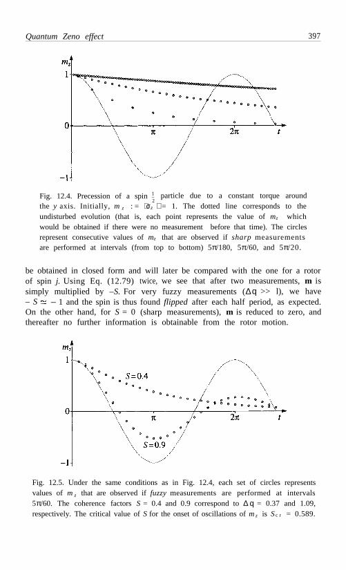
Quantum Zeno effect 397
Fig. 12.4. Precession of a spin 1–2
particle due to a constant torque aroundthe y axis. Initially, m z : = ⟨σ z ⟩ = 1. The dotted line corresponds to theundisturbed evolution (that is, each point represents the value of mz whichwould be obtained if there were no measurement before that time). The circlesrepresent consecutive values of mz that are observed if sharp measurementsare performed at intervals (from top to bottom) 5π/180, 5π/60, and 5π/20.
be obtained in closed form and will later be compared with the one for a rotorof spin j. Using Eq. (12.79) twice, we see that after two measurements, m issimply multiplied by –S. For very fuzzy measurements (∆q >> l), we have– S – 1 and the spin is thus found flipped after each half period, as expected.On the other hand, for S = 0 (sharp measurements), m is reduced to zero, andthereafter no further information is obtainable from the rotor motion.
Fig. 12.5. Under the same conditions as in Fig. 12.4, each set of circles representsvalues of m z that are observed if fuzzy measurements are performed at intervals5π/60. The coherence factors S = 0.4 and 0.9 correspond to ∆ q = 0.37 and 1.09,respectively. The critical value of S for the onset of oscillations of m z is S c r = 0.589.

398 The Measuring Process
A rotor with spin j
Obviously, a spin1–2 particle cannot mimic the classical rotor described by
Eq. (12.72). We therefore turn our attention to spin j. Let = 1, for brevity. We prepare the rotor in an eigenstate of Jz , with j z = j. We shall consideronly the “worst case scenario” mentioned above, with θ = π/2, so that the firstmeasurement of Jz is performed on an eigenstate of J x with eigenvalue j.
This rotation through an angle θ = π/2 is generated by a unitary matrix U .We have, with Wigner’s notations, 26
(12.81)
The probability of getting j z = m is the square of this matrix element. This isa binomial distribution with variance j/2. The result is shown in Fig. 12.6, forthe case j = 32 (the standard deviation then is ∆ J z = = 4).
Fig. 12.6. Expected probability distribution for a measurement of J z ,after preparation of a state with jz = j, and its rotation by π/2. Thecalculations were done for j = 32. The standard deviation is ∆Jz = 4.
The results of further measurements depend on whether the first measure-ment was sharp or fuzzy. If it was sharp ( S mn = δ mn ) the histogram of expectedresults for the second measurement (at θ = π) is given by the diagram at thetop of Fig. 12.7. The distribution is almost uniform, and very little informationcan be inferred from it. Better results are obtained if the first measurement wasfuzzy. The subsequent diagrams of Fig. 12.7 show the distribution of results ofthe second measurement, as a function of the ∆q of the meter which was usedfor the first measurement. Obviously, a very broad ∆q allows the quantumstate to reassemble near jz = – j, which would be its value at time t = π i fthe first measurement had not been performed.
On the other hand, if ∆q is too broad, the “measurement” becomes useless.Obviously, the expression which should be optimized is the one in Eq. (12.47).From the example discussed above, it appears that the fuzziness of the metershould be about the same as the natural width of the detector’s wave packet.A poorer resolution gives inaccurate and useless results, but a finer resolutiondestroys the information in which we are interested.
26 E. P. Wigner, Group Theory, Academic Press, New York (1959) p. 167.

Quanturn Zeno effect 399
Fig. 12.7. Expected probability distributions for a second measurementof J z , after one more rotation by π/2. The results depend on the ∆q o fthe meter which performed the first measurement. From top to bottom,this ∆ q (shown as a horizontal error bar) is 0, 1, 2, 4, and 8. Differentvertical scales are used in the various diagrams, for better visibility. Ineach diagram, the sum of lengths of the vertical bars is 1, by definition.
Exercise 12.6 Compute the data which are displayed in Fig. 12.7. You willneed the rotation matrix U = . Don’t use Wigner’s formula26 whichbecomes unwieldy for large j, because its result is the small difference betweenlarge terms with alternating signs. A better way of computing U is by means ofthe relationship UJz = J x U, which gives a recurrence relation between adjacentelements of the matrix U in the basis where Jz is diagonal.
The Zeno effect is a peculiarity of quantum physics. It disappears in thesemiclassical limit, when eigenvalues become extremely dense. From the quan-tum point of view, classical measurements are always fuzzy. This is why awatched pot may boil, after all: the observer watching it does not resolve theenergy levels of the pot. Any hypothetical device which would resolve these

400 The Measuring Process
energy levels would also radically alter the behavior of the pot. Likewise, themere presence of a Geiger counter does not prevent a radioactive nucleus fromdecaying. 18 The Geiger counter does not probe the energy levels of the nucleus:it interacts with its decay products whose Hamiltonian, including the kinetic en-ergy, has a continuous spectrum. As we have already learnt when we discussedthe implications of Bell’s theorem (pp. 183–185), quantum effects violate ourclassical intuition only when our instruments can resolve individual levels.
QND measurements and QND variables
A quantum nondemolition (QND) measurement is one performed on a systemwhich is known to be in one of the eigenstates of the measured operator. Thepurpose of such a measurement is to determine that eigenstate. All we haveto do is to perform a maximal test, with the basis defined by that operator. Ifthis is a repeatable test, the final state of the system is exactly the same as theinitial one, hence the label “nondemolition.”
A QND variable (sometimes called QNDD, for “quantum nondemolitiondetection” ) is on which satisfies [A (t ), A( t')] = 0. It is the quantum analog12
of a classical robust variable, as defined by Eq. (12.15). Such a dynamicalvariable can in principle be monitored continuously with arbitrary precisionwithout disturbing its evolution. For example, if v( t ) is a random classicalsignal, and if H = v (t )p, then q is a QND variable, because = v (t ), so that
(12.82)
and [q( t ), q( t ')] = 0. Measuring q will of course disturb p, but this has no effecton the evolution of q itself. Unfortunately, the Hamiltonian H = v( t )p is only amathematical construct, with no experimental counterpart.
Notice that QND variables have a continuous spectrum. This is intuitivelyobvious, since they have to follow a continuous evolution, and this can alsobe formally proved16 from the property [A( t ), A( t' )] = 0. It is unlikely thata nontrivial QND variable can actually be realized, because of the conflictingrequirements that it must satisfy: its time evolution should be sensitive to weakexternal signals, but on the other hand it should not be affected by the intenseinteraction needed for the measuring process.
12-6. Measurements of finite duration
Until now, I assumed that the interaction between the measuring instrumentand the observed system was almost instantaneous. The motion of the systemduring that time was ignored, and the measurement was simply representedby a unitary transformation, as in Eq. (12.3). This drastic simplification is

Measurements of finite duration 401
not always justified. Coupling constants occurring in nature are finite, andsometimes very small. It may therefore be necessary to couple the system andthe measuring apparatus during a finite, possibly long time. We shall nowexamine what happens during a measurement of finite duration.
As a first step, let us ignore the free Hamiltonians of the apparatus and of theobserved system, and consider only their interaction Hamiltonian, according tothe simple model in Eq. (12.39). Let the interaction start at time t = 0. Definean evolution parameter l ( t ) by
(12.83)
so that l (t ) gradually increases from 0 to its final value, 1, which is reachedupon completion of the measurement. The unitary transformation (12.40) nowbecomes a time-dependent relationship, with [q ± l( t)] instead of (q ± 1). Thewave function on its right hand side is just like the one that was sketched inFig. 12.3. An unfinished measurement therefore is a special case of a fuzzymeasurement, with a time-dependent coherence matrix: the eigenvalues λm inEq. (12.51) are replaced by λm l(t ).
Considering again the simple case of a measurement of σ z , the situation isdescribed by a density matrix:
(12.84)
, correlated tests on the spin –
where l = l (t ). The physical meaning of this expression is the usual one: Weimagine the existence of an ideal instrument which can instantaneously perform,at time t 1 particle and on the “pointer” which
2interacts with that particle. The density matrix (12.84) enables us to makestatistical predictions on the outcomes of these ideal tests. We have alreadyseen that if we completely ignore the pointer in such a correlated state, and wetrace out its coordinate q , the reduced density matrix of the spin –1 particle is
2given by Eq. (12.50). The only new feature now is that the coherence matrixS mn depends on time while the measurement proceeds.
There is however more to be said. 27 For example, we may ask pairs o fquestions, such as: “What is the probability of finding the pointer in a givenrange, q 1 < q < q 2 and, in that case, what are the properties of the spin?”To answer these questions, we have to delete from (12.84) all the values of qoutside the given range, and then to sum over q in that range:
(12.85)
27 A. Peres and W. K. Wootters, Phys. Rev. D 32 (1985) 1968.

402 The Measuring Process
1–The matrix R ( t) is analogous to a density matrix for the spin particle, but it2is not normalized to unit trace. Rather, its trace is the probability of findingthe pointer in the designated domain. The mean value of any spin variable Awhen the pointer is found in that domain is
(12.86)
Exercise 12.7 Show that R (0) is equal to the initial density matrix of theparticle, multiplied by the probability of finding the pointer between q1 and q2.
E x e r c i s e 1 2 . 8 Show that i f l(t) has become large enough so that the wavefunctions φ(q + l) and φ(q – l) do not overlap, the find R matrix for q > 0 is
(12.87)
What is the physical meaning of this equation?
Here, there should be no misunderstanding as to the nature of Eq. (12.85).The latter does not represent a dynamical process, and it cannot be generatedby a Hamiltonian, contrary to Eq. (12.3), for example. Equation (12.85) onlyformalizes the arbitrary selection of a given range of pointer positions, by anexternal agent which is not included in the dynamical variables.
Case Study: Stern-Gerlach experiment
As a concrete example, we shall follow the continuous time evolution of a Stern-Gerlach experiment, in which a particle prepared in an eigenstate of σx is testedfor σ z and the result is found to be 1, say. Assume for simplicity that g (t) inEq. (12.39) is a constant, and that the initial state of the pointer is given by
(12.88)
and φ( q ) = 0 elsewhere. The wave packets will separate, and the measurementbe complete, when l(t) = g t/ ≥ a. However, we are interested in the situationat earlier times, when l (t) < a and the two wave packets of the pointer stilloverlap. We ask: “What is the probability, at such a time t, of finding q > 0,and in that case, what are the properties of the spin?”
Initially, we have, with the same notations as above, α = β = 2 –1/2 . FromEqs. (12.84) and (12.85), we obtain
(12.89)
where b := l(t)/a < 1. It follows that

Measurements of finite duration 403
(12.90)
Exercise 12.9 Show that the eigenvalues of R (t ) are
(12.91)
and find the corresponding orthogonal eigenstates.
These results are shown in Fig. 12.8, where pairs of orthogonal eigenstates of Rare represented by vectors whose lengths are proportional to the correspondingprobabilities w j . These vectors point in opposite directions, since orthogonalstates in Hilbert space correspond to opposite spin polarizations. As expected,we have a continuous evolution between = 1 at the beginning of themeasurement, and = 1 at the end of the measurement.
1–2
1
Fig. 12.8. The initial, intermediate, and final states of the spin particle,during its evolution from = 1. The dots represent 20equidistant steps. At intermediate times, we have a mixture of orthogonalspin states, shown by opposite arrows. The length of each arrow is equalto the statistical weight of the corresponding state, given by Eq. (12.91).
The time dependence in Eq. (12.90) or, implicitly, in Eq. (12.89), is not thekind of evolution that can be followed, moment by moment, for a single spin –2particle. Quantum theory is fundamentally statistical. In order to observe thetime dependence illustrated by Fig. 12.8, one has to prepare a large numberof particles in the given initial state, divide them into 20 subsets (with a largenumber of particles in each subset), and let each subset evolve for a givenamount of time before observing its particles together with the correspondingpointers (there is one pointer for each particle, of course). Then, for each subset,

404 The Measuring Process
the statistical properties of the particles for which the pointer’s position wasfound positive are correctly described by Eqs. (12.89) and (12.90).
This new way of describing a time evolution is no more or less genuine thanSchrödinger’s equation. In both cases, one needs to prepare a large number ofidentical sets in order to observe the time dependence. The only difference isthat in the present example one cannot assign an evolution to a subensembleof particles until the observations “right vs left” have been made on the corre-sponding pointers.
1–
Measurement of time-dependent variables
2
We shall now examine what happens if we attempt to measure, in a way whichis not instantaneous, a dynamical variable which is not a constant of the mo-tion. This problem is not specific to quantum theory. It may arise in everydaylife, e.g., when a photographer takes a snapshot of a moving object. However,quantum theory introduces novel features, because a measurement is not onlya passive observation, but also the preparation of a new state. In particular,we shall see that the result of such a measurement is not, in general, the timeaverage of the observed quantity during the measurement.
In order to disentangle this problem from the preceding one, we shall nowconsider only measurements which have been brought to completion. As anexample, we want again to measure σz of a spin particle, but meanwhile, thelatter “wants” to precess with angular velocity 2ω around the x-axis, becauseits free Hamiltonian is ωσx . We thus have
(12.92)
Assume for simplicity that g (t) = T –1 is constant during the interval 0 < t < T,and vanishes at other times. The question that we address is the same as before:“Given the initial states of the particle and of the pointer, what is the probabilityof finding q > 0 at time t = T, and if so, what is the state of the particle?”(For t > T, the particle will continue to precess around the x-axis with angularvelocity 2ω. This is a trivial evolution which does not concern us.)
It is convenient, for this calculation, to use the momentum representationdefined by Eq. (10.54) for the state of the pointer. The operator p then becomesa c -number, p, and the evolution of the composite system, for 0 < t < T, isgiven by the unitary operator
(12.93)
For any value of p, this is simply a precession with constant angular velocity(2ω, 0, 2 p/ T ). Note, however, that the value of p is not sharp, because φ(q)ought to be a narrow wave packet, and therefore (p) is broad and differentcomponents of the state vector precess with different angular velocities. Thenarrower the wave packet is in q -space, the larger the values of p which are

The measurement of time 405
involved. In particular, if ∆q << 1/ωT, most of the wave function has p >>so that the precession axis is nearly aligned with the z-axis. In that case, adetailed calculation 27 shows that the free precession generated by ωσx is nearlystopped, even if T is large so that the coupling constant g is small (this in-cludes the case ωT > 2π). If we write the initial wave function as the sumof two components with definite σz , these components retain nearly constantamplitudes. This is just another example of the Zeno effect: the free part ofthe Hamiltonian, , is overwhelmed by the interaction term gpσz .
Exercise 12.10 Write the q-representation of U(p), and obtain the final wavefunction, for t = T, in q-space.
The answer to this exercise is a linear but nonlocal transformation,27 with akernel K(q – q ’) which has singularities at q = q’ ± 1, and continuous complexvalues between these two limits. Intuitively, this can be interpreted as follows:The pointer ought to move to the right or left, depending on whether σz = 1or –1. But σ z is not constant. A state with σz = ±1 will acquire componentswith σ z = 1, because of the precession ωσx . This causes the pointer tozigzag, and its final possible positions are not concentrated at q = ±1, butspread continuously between –1 and 1.
For a given final position of the pointer, what is the state of the spin? Ideally,we would want to have σ z = 1 if q > 0, and σ z = –1 if q < 0. Actually,the spin state is given by the reduced density matrix R (T), as explained above.Since the latter involves a nonlocal kernel, the particle is in a mixture of stateswith opposite spins. In particular, if we are using this imperfect apparatus toprepare two beams of particles with opposite polarizations, each one of thesebeams will be contaminated with particles of the wrong polarization.
These results are radically different from what could be expected on purelyclassical grounds, where an apparatus sensitive to σz would simply give the timeaverage of σz from t = 0 to t = T. In the quantum case, such a time averagecannot be directly measured with the simple apparatus described above, withconstant g(t). More sophisticated methods are however available, if we knowin principle the law of motion of the measured system, and our only task isto determine an unknown numerical parameter in that law. It is then possibleto tailor a time-dependent interaction Hamiltonian in such a way that, after aprescribed time, the position of a pointer will be correlated with the unknownvalue of that numerical parameter. Unfortunately, no general recipe is available,and each case must be treated ad hoc.
12-7 . The measurement of time
The measurement of time is different from that of quantities like position, mo-mentum, energy, etc., because time is not a dynamical variable. For example,a classical particle may have a well defined position, an energy, and so on, but

406 The Measuring Process
we cannot say that “a particle has a well defined time.” Formally, the Poissonbracket (in classical mechanics) or commutator (in quantum theory) of t withany dynamical variable is always zero.
What we call the measurement of time actually is the observation of somedynamical variable, the law of motion of which is known (and is usually uniform,like the motion of a pointer on a clock dial). For example, if we observe a freeparticle with classical Hamiltonian H = p ²/2m, the expression T = m q /psatisfies [T, H]PB = 1, and can therefore be considered as a “realization of time”(for that particular Hamiltonian).
Exercise 12.11 Show that the operator (in momentum representation)
(12.94)
satisfies the commutation relation [T,H] = i , and that the formal solution of
No simple physical meaning can be attributed to the results of the aboveexercise. If you want to try another exercise, take, instead of a free particle, aharmonic oscillator with H = 1 (p² + q ²). The result is even worse! In classical
2mechanics, you can define T = tan –1 (q/p), which is multiple valued, just likethe hour on an ordinary watch. But there is no such thing as a “multiple valuedoperator” in a correctly defined Hilbert space.
–
Larmor clock
A simple quantum clock28–30 can be produced by using the finite-dimensionalquantum dial discussed on page 320 as a basis for quantizing the continuousrotor clock that was introduced in Sect. 12-2. The clock’s Hamiltonian is
(12.95)
Its eigenstates um are, in the q -representation, with m = –j, . . . , j.The complementary basis is
(10.89)
where N = 2j + 1. The vectors vµ are called dial states.The clock has a time resolution
(12.96)
28H. Salecker and E. P. Wigner, Phys. Rev. 109 (1958) 571.29 M. Büttiker, Phys. Rev. B 27 (1983) 6178.30 J. P. Falck and E H Hauge, Phys. Rev. B 38 (1988) 3287.. .
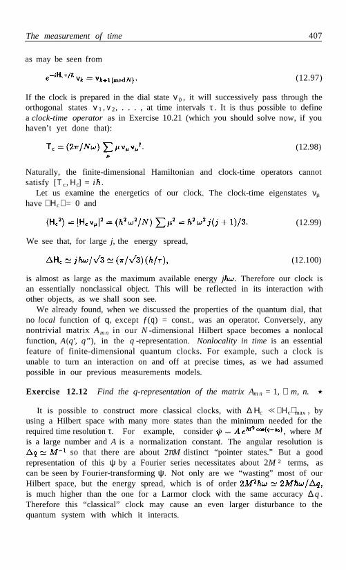
The measurement of time 407
as may be seen from
(12.97)
If the clock is prepared in the dial state v 0 , it will successively pass through theorthogonal states v 1 , v 2, . . . , at time intervals τ . It is thus possible to definea clock-time operator as in Exercise 10.21 (which you should solve now, if youhaven’t yet done that):
(12.98)
Naturally, the finite-dimensional Hamiltonian and clock-time operators cannotsatisfy [T c, Hc] = i .
Let us examine the energetics of our clock. The clock-time eigenstates vµ
have ⟨ Hc ⟩ = 0 and
(12.99)
We see that, for large j, the energy spread,
(12.100)
is almost as large as the maximum available energy j . Therefore our clock isan essentially nonclassical object. This will be reflected in its interaction withother objects, as we shall soon see.
We already found, when we discussed the properties of the quantum dial, thatno local function of q, except ƒ(q) = const., was an operator. Conversely, anynontrivial matrix Am n in our N -dimensional Hilbert space becomes a nonlocalfunction, A(q', q”), in the q -representation. Nonlocality in time is an essentialfeature of finite-dimensional quantum clocks. For example, such a clock isunable to turn an interaction on and off at precise times, as we had assumedpossible in our previous measurements models.
Exercise 12.12 Find the q-representation of the matrix Am n = 1, ∀ m, n.
It is possible to construct more classical clocks, with ∆ Hc << ⟨ Hc⟩ max , byusing a Hilbert space with many more states than the minimum needed for therequired time resolution τ. For example, consider , where Mis a large number and A is a normalization constant. The angular resolution is
so that there are about 2πM distinct “pointer states.” But a goodrepresentation of this ψ by a Fourier series necessitates about 2M ² terms, ascan be seen by Fourier-transforming ψ. Not only are we “wasting” most of ourHilbert space, but the energy spread, which is of orderis much higher than the one for a Larmor clock with the same accuracy ∆ q .Therefore this “classical” clock may cause an even larger disturbance to thequantum system with which it interacts.

408 The Measuring Process
Time-of-flight measurement
A quantum clock can be used for measuring the time of passage of a particlebetween two detectors, by coupling that clock to the translational degree offreedom of the moving particle. In particular, the clock can keep a permanentrecord of the time of flight, which can be read long after the process has beencompleted, as we shall now see.
The simplest way of achieving this is to have the movement of the clockactivated when the particle passes through the first detector, and stopped whenit passes through the second one. Let x1 and x 2 be the positions of thesedetectors, and x be the position operator of the particle (recall that q is thepointer position on the clock dial). Define, in the x -representation, a projector
(12.101)
A suitable Hamiltonian for the particle (mass m ) and the clock is
(12.102)
so that the clock runs only when the particle is located between the detectors.Both H and Hc are constants of the motion. The initial state of the clock is thedial state . However, it is easier to solve the equations of motionif the clock is in an eigenstate of Hc , say u n , and then to sum the solutions forall n, so as to get the solution corresponding to the initial state v0 .
If the state of the clock is un , the operator H c can be replaced by the numericalconstant n ω, and the Hamiltonian (12.102) simply represents a particle ofmass m with a potential barrier of height V = n ω and length L = x 2 – x 1 .Outside the barrier, the wave number is k = (2mE)1/2 , where E = p²/2mis the constant value of H. Inside, it is k' = [2m(E – V)]1/2 / . Therefore thephase shift caused by the barrier is
(12.103)
where the right hand side is an approximation valid for V << E. Note thatv = ( 2E/m)1/2 is the classical velocity of the particle, so that L/v is the classicaltime of flight T. Thus, if the incoming wave function (before the barrier) is
(12.104)
the outgoing vave function (after the barrier) is
(12.105)

The measurement of time 409
The pointer, which was initially directed toward q 0, ends up oriented towardq ωT. It correctly indicates the time of flight between the detectors.
It is remarkable that this derivation never assumed that the particle wasconstrained to stay in a wave packet much smaller than L, or in general thatit passed through each detector at a definite time. We wanted to measure onlythe time interval between the two detectors. The latter is perfectly well definedby the initial momentum p = k, even though the times of passage througheach detector are completely uncertain.
Our only assumption was that V << E, so that the disturbance causedby the measurement is small. Since V can be as large as , itfollows that τ >> /E. This imposes a lower limit on the time resolution of theclock, which in turn causes a limitation of the accuracy with which the particlevelocity can be measured over a distance L :
(12.106)
which can also be written as ∆ p >> /L. This result should not be construedas another Heisenberg uncertainty relation. It rather is an inherent limitationof our time-of-flight method for measuring the velocity of a particle. It is ofcourse quite possible to measure p with arbitrary accuracy by other methods.
When did the atom decay?
When did Schrödinger’s cat die? Instead of the legendary cat, consider aquantum clock which runs as long as the radioactive atom has not decayed.The question becomes: When did the clock stop?
Let us compute the location of its pointer when t → ∞. As the Hamiltonian,take
H = H a + P 0 Hc , (12.107)
where H a is the Hamiltonian of the radioactive atom, P0 is the projector onthe atom’s initial state φ0 , and H c = , as before. We split H a = H 0 + V,where H0 has both a discrete spectrum (and in particular it has an eigenstateφ0 corresponding to the energy E 0 ) and a continuous spectrum in a domainwhich includes E0 . For example, φ0 may be an excited state of the atom, whilethe continuous spectrum corresponds to its ground state accompanied by oneor more photons of arbitrary energy. To simplify the discussion, let us assumefor a moment that the atom is enclosed in a large box, so that the continuousspectrum becomes discrete and consists of normalizable states φE , with a coarsegrained density ρE . All these states are mutually orthogonal.
A further simplification of our model is to assume that the only nonvanishingmatrix elements of V are
(12.108)

410 The Measuring Process
and that these matrix elements have a slow dependence on E. Under theseassumptions, it can be shown31 that, in the wave function
(12.109)
the coefficient of the initial state φ0 decays in an approximately exponentialway: a 0 . Substitution of this result in Schrödinger’s equation
(12.110)
gives a E ( t ) explicitly. In particular, for t → ∞, we have
(12.111)
so that
(12.112)
Conservation of the norm (namely, ⟨ψ, ψ⟩ = 1) implies that
(12.113)
from which we shall now obtain the actual value of γ.First, we must examine how the above infinite sums behave when the volume
of the box, which we shall denote as Ω , increases to infinity. If the normalizedeigenfunctions φE are not localized, their amplitude behaves as Ω –1/2 . This alsois therefore the behavior of ⟨φE , V φ0 ⟩ , if the initial wave function φ0 is localized.The expression V ( E ) := Ω1/2 ⟨φE ,V φ0⟩ thus tends to a limit (a smooth functionof E ) as Ω → ∞. Likewise, the density of states ρ (E) := ρ E /Ω tends to asmooth limit. We can therefore rewrite Eq. (12.113) as
(12.114)
Thus, since the functions ρ(E) and V (E) are almost constant over a domainmuch larger than γ, it follows from (12.114) that
(12.115)
which is Fermi’s golden rule.Let us now couple our atom to a clock, as in Eq. (12.107). The clock’s initial
state is , but we shall again solve the problem for a clock in aneigenstate u n , so that H c can be replaced by the numerical constant . Theonly change in the Hamiltonian H is that the energy of the initial state φ0 hasbeen shifted from E0 to E 0 + . This may modify the value of γ in (12.115),but the new decay constant will still be very close to the old one, as long as
31A. Peres, Ann. Phys. (NY) 129 (1980) 33.

The measurement of time 411
(12.116)
We again obtained a lower limit on the time resolution of the clock:
(12.117)
A time resolution which is finer than this expression will alter the decay law(and in the limit τ → 0, a Zeno effect will occur, of course).
In what follows, it will be assumed that we have kept the clock energy lowenough, and therefore the time resolution poor enough, so that the inequality(12.117) is fulfilled and the decay law is not appreciably affected by the clock.For t → ∞, the combined state of the atom and the clock is given by Eq. (12.112)with E 0 → E 0 +
(12.118)
We are now going to observe the clock, but not the decay products of the atom.Therefore the state of the clock (more precisely, the statistical properties ofan ensemble of clocks which have been subjected to the same experiment) isrepresented by the reduced density matrix obtained from the state (12.118) bytracing out the degrees of freedom of the atom:
(12.119)
In this partial trace, we pass to the continuum limit:
(12.120)
This gives
(12.121)
(12.122)
Both functions in the numerator were assumed very smooth, and their productcan therefore be replaced by the constant γ/π, defined in Eq. (12.115). We canthen safely extend the integration limits to ± ∞ . We obtain
where is the angle through which the pointer of a classical clockwould turn during the average atom lifetime,
We can now compute the probability for finding a clock stopped at timeThis probability is pµ = , or

412 The Measuring Process
(12.123)
This double sum can be evaluated explicitly32 and gives, for large N,
(12.124)
Exercise 12.13 Let θ = 2πµ/N be the angle on the dial that correspondsto time tµ . If µ < 0, redefine µ → µ + N, so that 0 ≤ θ < 2 π. Show that theright hand side of Eq. (12.124) is the Fourier series expansion of
(12.125)
We see from this exercise that the clocks stop (the atoms decay, the cats die)at times distributed according to the familiar exponential decay law, with dueaccount taken of the fact that a clock may run through more than one cyclebefore stopping. Quantum theory, which makes only statistical predictions, isof course unable to specify when an individual atom will decay, or an individualcat will die.
Switching interactions on and off
A clock can be used not only to measure, but also to control the duration ofa physical process. We shall now see how an interaction can be switched onat a preset time t a , and then switched off at time tb . For instance, this inter-action may involve a magnetic field which causes the precession of a spin 1
2particle. The problem is to write a time-independent Hamiltonian, such thatthe precession angle increases linearly between ta and t b
–
.Various models can be devised, which have that effect. If we still want to use
a Larmor clock, we may write
(12.126)
where Ω denotes the spin precession velocity. As usual, the translational degreesof freedom of the spinning particle have been ignored. Following the sametechnique as before, we take initial states which are eigenstates of the constantof motion σ z . We can then replace, in Eq. (12.126), the operator σ z by ±1,and thereby obtain an expression which involves only the clock. On the otherhand, H c is not a constant of the motion, because it does not commute withthe projectors vµvµ
†. We see that using a clock to control a process perturbsthe clock mechanism! Are you surprised?
The equations of motion of the clock can be soved by perturbation theory.The calculations are fairly intricate32 and will not be reproduced here. The endresult is that the precession angle is approximately given by the ramp function
3 2A. Peres, Am. J. Phys. 48 (1980) 552.

Time and energy complementarity 413
(12.127)
This is the desired result. It was obtained by using the time-independent Hamil-tonian (12.126). The approximations that are needed for the derivation of thisresult are j >> 1 (which is necessary for making a good clock) and Ωτ << 1,which means that the clock’s time resolution is much finer than the precessionperiod—a physically obvious requirement. 32
–
Another, more realistic model for switching on and off a magnetic field is touse as our clock the translational degree of freedom of the spin 1
2 particle, whichsimply enters into a magnet at time ta , and exits at time tb . The Hamiltoniandescribing this model is similar to the one that was used for the time-of-flightmeasurement:
(12.128)
Comparing this with Eq. (12.102), we see that the spin and position degrees offreedom have exchanged their roles. The solution of the equations of motion isthe same, of course (in the present case, j = 1
2).–
Exercise 12.14 Show that the condition V << E that was necessary for thetime-of-flight measurement becomes now
(12.129)
where and L is the length of the magnet. What is the physical meaningof this condition?
12-8. Time and energy complementarity
It is well known that time and frequency are conjugate variables in a pair ofFourier transforms. As a consequence, the duration of a signal (a musical note,say) and the frequency of that signal (the pitch of the note) are subject to anunsharpness relation, ∆ t ∆ω ≥ 1
2 . This property, illustrated in Plate III (page214), is purely classical.
–
In quantum theory, frequency means energy. You find, in some textbooks andarticles, an uncertainty relation ∆ t ∆ E ≥ or, even worse, a “relativistic”generalization:
(12.130)

414 The Measuring Process
What can be the meaning of such a relation? In conventional quantum theory,/2 means that if we measure q on an ensemble ofthe statement ∆ q ∆ p ≥
particles, and p on another identically prepared ensemble, the product of thestandard deviations of the results of these measurements is at least /2. If wetry to interpret (12.130) in the same way, we are faced with two difficulties: It isin general wrong that ∆ x ∆ H = 0, since x is not a constant of the motion; andthe expression ∆t is undefined, because there is no t operator, and no meaningcan be given to “measuring the time of a physical system,” in the same way aswe measure its position, or momentum, etc.
Another claim which frequently appears in the literature is the following:If δt is the duration of the measurement of an energy, the result is uncertainby . This claim is absurd. It is analogous to saying that if wemeasure a momentum with an apparatus of size δx, the momentum uncertaintyis . This is manifestly wrong: a mundane radio receiver whose sizeis only a few centimeters can determine the wavelength of a radio station withan accuracy ∆λ /λ << 1. In other words, it measures the momentum of thephotons emitted by that station with an accuracy
(12.131)
Still another claim, illustrated in Plate I (page 2), is that the time (registeredby a clock) at which an energy is measured with an accuracy ∆E, is uncertainby at least / ∆E. This already sounds better, because we have defined a clock-time operator T c, and we can therefore investigate the possible existence of anuncertainty relation between ∆T c and ∆ H. However, there is no reason toexpect that there actually is such an uncertainty relation, because the operatorT c refers to the clock, and the operator H to the observed system. These twooperators commute, and quantum theory allows us, in principle, to measureboth of them simultaneously with arbitrary accuracy. The analogy with a radioreceiver can again be used: its position can be accurately determined while itmeasures the momentum of the photons emitted by the radio station, in sucha way that Eq. (12.131) is easily satisfied.
These issues were not understood in the early years of quantum theory. It isonly at much later stage that they were thoroughly analyzed by Aharonov andBohm, 33 who came to the conclusion that “there is no reason inherent in theprinciples of quantum theory why the energy of a system cannot be measuredin as short a time as we please.” To support their claim, Aharonov and Bohmconstructed a model Hamiltonian, involving two particles (the “system” and the“apparatus”), such that the apparatus could perform a repeatable measurementof the energy of the system in an arbitrary short time.
These conclusions were criticized by Fock,34 on the grounds that the Hamil-tonian used by Aharonov and Bohm contained an arbitrarily sharp function oftime, g(t), for switching on and off the interaction. Fock wrote:
33Y. Aharonav and D. Bohm, Phys. Rev. 122 (1961) 1649.34 V. A. Fock, J. Exp. Theor. Phys. (U.S.S.R.) 42 (1962) 1135 [transl.: Soviet Phys. JETP 15
(1962) 784].

Time and energy complementarity 415
The introduction of an explicitly time-dependent interaction is equivalentto the introduction of a field which can be described classically (in the cor-respondence principle sense). However, the classical fields and test bodiesused in the equations of quantum mechanics are not free of the limitationsimposed by the Heisenberg uncertainty relations. On the contrary, the useof classical fields and test bodies is based on the premise that the uncer-tainty relations are satisfied for them so strongly [i.e.,∆ q ∆ p >> ] thatit is unnecessary to introduce these relations explicitly. If however it is(illegimately) assumed that the classical field or test particle may violatethe Heisenberg relations, it should come as no surprise that these relationswill also be violated for the quantum mechanical particle serving as object.
To counter Fock’s criticism, Aharonov and Bohm35 modified their Hamiltonianby introducing a third particle (a “clock” with linear coordinate z) and replacedthe switching function g(t) by a time-independent function, g (z ). The resultingtime-independent Hamiltonian formally allowed to measure the energy of thesystem, repeatably and in an arbitrarily short time. Everything in this modelwas internally consistent.
This still leaves an open question, namely whether there are, in nature, inter-actions which are arbitrarily intense and localized, like the function g(z). In thepresent context, however, this is a practical problem, not a fundamental one. Itis like asking, when we study Euclidean geometry, whether it is possible to drawarbitrarily thin lines, or to manufacture perfectly rigid rulers and compasses.These technical questions are irrelevant to the study of geometry. Likewise, thepractical feasibility of producing in a laboratory the Hamiltonian that we havewritten (without violating any fundamental law, of course) is irrelevant to thelogical structure of quantum theory.
of rulers and compasses. How good a simulation we can actually achieve is animportant practical problem, but not a fundamental one.
When we analyze these fundamental issues, we should not consider quantumtheory as a tool with which we describe existing physical objects. Rather, quan-tum theory must be seen as a set of abstract rules—just as Euclidean geometry.When we come to the physical interpretation of the theory, its abstract elementsare simulated by material objects—just as the abstract notions of “line” and“circle” are simulated by thin dark bands drawn on white paper with the help
Metastable states
The survival probability of a time-dependent quantum state is defined as
(12.132)
(The word “survival,” used in the current literature, is somewhat misleading,as it suggests the irreversible death of a member of a living community. No
35 Y. Aharonov and D . Bohm, Phys. Rev. B 134 (1964) 1417.

416 The Measuring Process
irreversible phenomena are involved in the discussion below, and there is noreason for the “survival probability” P( t ) to be a monotonic decreasing functionof time. It may also temporarily increase, or oscillate, as in the periodic motionof a coherent state of a harmonic oscillator.)
Exercise 12.15 L e t (0) = ∑ c u , where uE E E denotes energy eigenstates.Show that
Exercise 12.16 For systems with a continuous spectrum, the result ofthe preceding exercise becomes Therefore
a n d w (E ) are a pair of Fourier transforms. Show that the expo-nential decay law, corresponds to
(12.133)
where E1 is the mean energy of the metastable state, and
The energy distribution in Eq. (12.133) extends to and in particular hasan infinite ∆E. This is obviously unphysical. Therefore, no decay law canbe strictly exponential. It can however be shown 31 that P (t ) decays in anapproximately exponential fashion, provided that
(12.134)
where E 0 is the ground state of the system. Note in particular that γ, which isthe half-width of the resonance curve (12.133) at half its maximum height, isnot the same thing as ∆E, the standard deviation of the energy distribution. Inperturbation theory, γ is a second order quantity, as shown by Fermi’s goldenrule (12.115), while ∆ E = is of first order.
Deviations from the exponential decay law are most noticeable for very shorttimes, as may be seen by expanding Eq. (12.132) into powers of t. We have
(12.135)
A more accurate formula is36
(12.136)
which is easily proved as follows: 37 For any operator A we have, by virtue ofthe uncertainty relation (4.40),
(12.137)
In particular, let A be the projector on the initial state ψ (0). We then have
36 G. N. Fleming, Nuovo Cimento A 16 (1973) 232.37 D. Home and M. A. B. Whitaker, J. Phys. A 19 (1986) 1847.

Incompatible observables 417
Moreover, A 2 = A, so that
Combining these equations, we obtain
(12.138)
(12.139)
(12.140)
and Eq. (12.136) follows, by a trivial integration.
12-9. Incompatible observables
Let us try to measure simultaneously noncommuting operators A and B, b ygeneralizing the interaction (12.39) as follows:
(12.141)
where p1 and p 2 refer to two independent pointers. To simplify the analysis,let g (t) = 1 for the duration of the interaction (0 < t < 1 with an appropriatechoice of the time unit). The result of the interaction (12.141) is most easily seenin the Heisenberg picture or, equivalently, in classical mechanics, with Poissonbrackets instead of commutators. The equations of motion are
(12.142)
and
(12.143)
In classical mechanics, we can always assume that p1 = p 2 = 0, and it thenfollows from (12.143) that A and B are left undisturbed by the measuringprocess. In quantum theory, the situation is more complicated. We want thepointers to be well localized. Their wave functions φ1(q1 ) and φ2(q2 ) must havenarrow support, so that the expectation values of the displacements,
and
are not marred by large dispersions.

418 The Measuring Process
However, a narrow support for ( q) entails a broad distribution for the cor-φresponding momentum representation, ( p ). It then follows from (12.143) thatA and B do not remain constant during the measuring process. The measure-ments disturb each other, and the final meter readings, given by Eq. (12.144),do not represent the initial nor the final values of A and B, but rather somemean values, during the interaction.
Positive operator valued measures
A more sensible way of getting information about incompatible observables isto use a non-orthogonal POVM, as in Eq. (9.79). The resulting information willnecessarily have some fuzziness, as we shall explicitly see in the example below,but this is the best that can be done in a quantum context.
What is a good POVM? A natural requirement is the following one: if thesystem was prepared in such a way that A has a sharp value (a fact which couldbe ascertained by a von Neumann measurement of A), the POVM shall give usa good estimate of that value; and if the system has a sharp value of B, thesame POVM gives a good estimate of the value of B. This criterion is in generalagreement with the classical meaning of the word “measurement,” but it alsoallows for some uncertainty of the results, as demanded by quantum theory.
Conversely, the selection (by a quantum test) of a particular component of thePOVM should be equivalent to the preparation of a mixed state for which bothA and B have roughly defined values. We have already seen an example of thisproperty on page 386, where a POVM is used for the approximate determinationof an angular momentum coherent state.
Exercise 12.17 Set up, by analogy with Eq. (12.37), a POVM which allowsto measure approximately q and p.
A simple, intuitive method for the simultaneous measurement of q and p wasproposed by Arthurs and Kelly.
38,39Consider an ancilla, with canonical variables
Q and P, prepared in a standard coherent stateΨ0 , with ⟨ Q⟩ = ⟨ P⟩ = 0, and∆ Q ∆ P= /2. The dynamical variables q – Q and p + P commute and cantherefore be measured simultaneously.
Before this measurement, the state of the composite system is a directproduct, The expected dispersion of the possible results of themeasurement is
(12.145)
and likewise for ∆ (p + P). If initially ∆ q ∆Q, we have ∆ (q – Q ) ∆ Q, Sothat the observed value of q – Q typically differs from the sharp value of q byabout ∆ Q. Conversely, if initially ∆ p ∆ P, we have ∆ (p + P) ∆P, and
38 E. Arthurs and J. L. Kelly, Jr., Bell System Tech. J. 44 (1965) 725.39 S. Stenholm, Ann. Phys. (NY) 218 (1992) 233.

Incompatible observables 419
the observed value of p + P may differ from the sharp value of p by about ∆P .The criteria for a good POVM are therefore satisfied.
It is instructive to write explicitly the POVM which corresponds to the aboveprocedure. Let x = q–Q and y = p+P. These are a complete set of commutingoperators, and a pure state of the composite system can be denoted as Φ ( x , y).Let us divide the classical xy plane into small rectangular cells Cµ , centered at(x µ ,yµ ), and covering the entire plane. The determination of a particular valueof the label µ is equivalent to a measurement of x and y, with a resolution equalto the size of the cell Cµ .
Let us define functions
if x ∈ Cµ,otherwise,
andif y ∈ Cµ,otherwise.
(12.146)
(12.147)
Further define which satisfies and
(12.148)
In quantum theory, the Ι Ι µ (x,y) are a complete set of orthogonal projectors,which correspond to the possible outcomes of a von Neumann measurement.If the initial state of the composite system is Φ, the probability of obtainingoutcome µ is
(12.149)
Obviously, the most convenient way of expressing is its coordinaterepresentation, namely Likewise, is most easilywritten by means of the momentum representation, asThe inner product (12.149) is thereby referred to two different bases. This doesnot cause any difficulty. For example, if we have
(12.150)
where C m µ is the unitary matrix relating the bases u m and v . Likewise,µ
given the wave functions φ(q) and (p), we have, from the definition of themomentum representation, Eq. (10.54),
(12.151)
The value of ⟨Π µ⟩ , given by Eq. (12.149), thus becomes

420 The Measuring Process
To evaluate this expression, replace the integration variables q, p, Q, and P,by q, p, x = q – Q, and y = p + P (the Jacobian of the transformation is 1).The integrations over x and y are trivial if the cell C µ is small enough so thatthe other functions in the integrand can be considered as constant within thatcell: we simply replace, everywhere in the integrand, x by x µ , and y by y µ .Denoting the cell area by S µ (which has the dimensions of an action) we obtain
(12.152)
This factorization is remarkable! Consider in particular the initial state ofthe Arthurs-Kelly composite system, namely where
(12.153)
is a coherent state centered at Q = P = 0. We have, in (12.152),
(12.154)
Now, it is readily seen from Eq. (10.99) that
(12.155)
is the result of displacing 0(q), so as to obtain a new coherent state, µ (q),centered at the point (x µ yµ). Therefore (12.154) becomes
(12.156)
Exercise 12.18 Show that the momentum representation of the minimaluncertainty wave packet (12.155) is
(12.157)
and that
(12.158)
Using the results of this exercise, we finally obtain
(12.159)
where the POVM element A µ is proportional to the projector on the coherentstate µ,
(12.160)
Incompatible observables 421
The WAY theorem
Until now, we considered pairs of incompatible observables, represented by non-commuting operators. It was tacitly assumed that any single given operatorcould always be measured, by concocting an interaction Hamiltonian like theone in Eq. (12.39). We shall now examine this assumption more carefully.Quantum theory, by itself, does not preclude the realizability of an arbitraryHamiltonian. However, additional requirements may restrict the class of ad-missible interactions. In particular, we may demand that specific conservationlaws be respected during the measuring process.
For example, let p be the momentum of the observed system, and P that of themeasuring apparatus. If there is no external agent to carry excess momentum,p + P is conserved. This precludes the measurement of any dynamical variable,such as q , that does not commute with p + P (to measure q , there shouldbe a term involving q in the interaction Hamiltonian, and then p + P wouldnot be constant). The reason for this is simple: Conservation of the totalmomentum implies that we live in a translation invariant world, where the originof the coordinates is not a physical object. Therefore, the position operator qis experimentally meaningless. Only the relative position of the system withrespect to the apparatus, q – Q, is observable, and indeed q – Q commuteswith p + P, and can be measured without violating any conservation law.
More generally, the WAY theorem 40, 41 states that it is impossible to measure(in the von Neumann sense) an operator which does not commute with anadditive conserved dynamical variable. A simple proof 42 is given below.
Let A and B be two operators belonging to the observed system, and C anoperator of the apparatus, having the property that the sum B+C is conserved.In particular, if U is the unitary operator which produces a measurement of A ,we have
(12.161)
Recall that such a measurement generates a correlation of the eigenstates of A(which are defined by Aum = m um ) with various states vmα of the apparatus,as in Eq. (12.3):
(12.162)
The last equation defines wm , which satisfies = 1, by unitarity.We have to show that A cannot be measured unless [A, B] = O. Indeed, in
the basis um , which diagonalizes A, we have
(12.163)
40E. P. Wigner, Z. Phys. 133 (1952) 101.41 H. Araki and M. M. Yanase, Phys. Rev. 120 (1960) 622.42 G. C. Ghirardi, F. Miglietta, A. Rimini, and T. Weber, Phys. Rev. D 24 (1981) 347, 353.

422 The Measuring Process
Moreover, [A, C] ≡ O, because A belongs to the observed system, and C to theapparatus. The matrix elements in (12.163) can therefore be written as
(12.164)
Combining these various equations, we obtain, for m ≠ n,
(12.165)
since ⟨um , un
⟩ = 0. It follows that either ⟨wm , wn
⟩ = 1, which effectively meansthat there is no measurement, or Bmn = 0, which implies [A, B] = O.
Nonetheless, an approximate measurement of the operator A is possible,41,42
provided that the initial state of the apparatus has a sufficiently large value of∆C. For instance, if we want to measure q but we can only measure q – Q,we shall prepare the apparatus in a state with a very narrow ∆ Q. Then theobserved value of q – Q will typically differ from the expected value of q (whichwe cannot directly observe) by a quantity of order ∆ Q. Therefore ∆Q, which isdefined as usual as the standard deviation of Q in the initial state, also acquiresthe meaning of an uncertainty in the inferred value of q. Obviously, in such aprocedure, the initial state of the apparatus has a large ∆ P.
Here is another example: the WAY theorem implies that, if the total angularmomentum is conserved, we can only measure rotational scalars. Then, howcan we measure µz in a Stern-Gerlach experiment? This is the z-component of avector operator, which does not commute with the conserved rotation generatorsJx and J y . Yet, we can approximately measure µz . The point is that µz appearsin the Hamiltonian (1.4), which describes the Stern-Gerlach experiment, only inthe combination µµ ..B . This indeed is a rotational scalar, which can be measuredwithout violating any conservation law. The true problem is to guarantee thatB, the magnetic field at the location of the atomic beam, precisely points towardan externally defined z-direction.
To give the desired orientation to the magnetic field, the magnet has tobe prepared in a superposition of many different angular momentum states.We have already encountered this property with a much simpler system, theN-state quantum dial of Sect. 12-7. Each dial state (10.89) has an angularresolution α = 2π/N and its angular momentum spread, given by (12.100), is∆J = Moreover, for a macroscopic body such as a Stern-Gerlachmagnet, a given angular resolution α entails a value of ∆J considerably largerthan /α (see Fock’s remark on uncertainty relations for classical bodies, quotedon page 415). Thus, if we set an upper bound to ∆J, the WAY theorem impliesthat, instead of measuring σz , we actually measure some other component, σn ,along a direction n which is slightly different from the required direction z.
Exercise 12.19 For given values of J and ∆ J , estimate the expecteddeviation of n from the z-axis.

Approximate reality 423
12-10. Approximate reality
Quantum theory is not an objective description of physical reality. It only pre-dicts the probability of occurrence of stochastic macroscopic events, followingspecified preparation procedures, such as, for instance, the triggering of particledetectors following the collision of a specified beam with a given target. Thesetheoretical predictions rely on conceptual models which involve elusive micro-scopic objects, such as electrons, photons, etc. The latter are usually consideredas real things, but they occasionally display extraordinary nonlocal properties,quite at variance with intuitive classical realism, as we have seen in Chapter 6.
The essential difference between these two classes of objects, microscopic andmacroscopic, is not a matter of size, but of the completeness of their description:all the degrees of freedom of a quantum system are taken into account in itsHamiltonian. On the other hand, only a very small fraction of the degreesof freedom of a macroscopic system (a few of them, out of 10
20or 10 30 ) are
explicitly used in its description. We renounce keeping track of nearly all thephysical properties of macroscopic systems. These are open systems: the degreesof freedom that are not explicitly taken into account play the same role as anexternal environment. (There also are intermediate, mesoscopic objects, forwhich a significant fraction, but not all, of the degrees of freedom are explicitlydescribed.)
Since we give only an incomplete description of an open system, it is temptingto postulate that some of its operators are not measurable. For example, let uand v denote two opposite magnetization states of a macroscopic ferromagnet.The operator is observable (with eigenstates u and v) but, on theother hand, the Hermitian operator is not. The eigenstates of Mx
are , namely coherent superpositions of u and v magnetizations—or,if you prefer, of live and dead Schrödinger’s cats. Even if such superpositionscould be prepared, we would be unable to maintain their coherence for anappreciable time, as the following exercise shows.
Exercise 12.20 A compass needle containing 1 020 electrons with alignedspins is placed in a magnetic field which is stabilized with an accuracy of±10–9 gauss. How long does it take for the phase difference between the uand v states to become completely uncertain? Ans.: ~ 10–17 s .
The situation illustrated by this exercise is a special case of the emergence of“pointer states”: 43 the relevant degrees of freedom of each macroscopic systemdefine a preferred orthogonal basis (such as u and v in the above example, or Land D for Schrödinger’s cat). The elements of that basis are called pointer statesand have the property of being stable, except for an overall phase, with respectto small, uncontrollable fluctuations of the environment. On the other hand,linear combinations of pointer states have essentially non-classical properties
43 W. H. Zurek, Phys. Rev. D 24 (1981) 1516; 26 (1982) 1862.

424 The Measuring Process
and are experimentally inaccessible. Their interaction with the environmentrapidly transforms them into incoherent mixtures.
Admittedly, the above claims of impossibility are no more than heuristicrules. They cannot be formulated, let alone proved, in any rigorous way. Thereis nothing in formal quantum theory which indicates that linear combinationssuch as can be prepared for single particles, or for pairs of particles,but not for 10, or 1010 identical particles. You should never underestimate theskill of experimental physicists!
Assuming that we have set arbitrary rules for distinguishing measurable fromnonmeasurable operators, it is then possible to define a classical system as aspecial type of quantum system, for which all measurable operators commute. 44
All the observable properties of such a classical system are compatible and cantherefore have sharp values. Note that a “classical” system defined in this waymay also have noncommuting operators, but the latter should be consideredas abstract mathematical expressions, which are not experimentally observ-able. With this formal definition, the notion “classical” acquires a meaningwith respect to a specified set of dynamical variables. Obviously, by usingfine enough observation means, every physical system will display quantumfeatures.44 Physics is not an exact science. It is a science of approximations.
Macroscopic objectivity
Real life seldom follows the idealized preparation-observation pattern presentedthroughout this book. Astronomers, for instance, observe spectral lines (i.e., d e -tect photons) which they interpret as due to the presence of atoms or moleculesin interstellar space. Obviously, the atoms were there a long time ago in anexcited state; they decayed to their ground state, emitting photons which wecan now observe, considerably later. These excited atoms were not prepared byus, nor our research assistants. We can only observe them passively. We alsoobserve bigger objects, such as the Moon moving around the Earth, or variousplanets, without ever having prepared them.
This would cause no conceptual difficulty with quantum theory if the Moon,the planets, the interstellar atoms, etc., had a well defined state ρ. However,I have insisted throughout this book that ρ is not a property of an individualsystem, but represents the procedure for preparing an ensemble of such systems.How shall we describe situations that have no preparer?
Let us formulate the problem more precisely. Until now, we were interestedin questions of the type answered by Eq. (9.79): “Given a preparation ρ, whatis the probability for an observation A µ?” (the µ-th element of a POVM).Now, there is a different type of question. For example, we may ask what isthe probability that if astronomer A successfully detects a POVM element Aµ(e.g., observes a dot on his photographic plate, which he interprets as a star)then another astronomer, B , will likewise detect a definite POVM element Bn .
44J. M. Jauch, Helv. Phys. Acta 37 (1964) 293.

Approximate reality 425
To make these observations causally independent, let them occur in mutuallyspace-like regions (simultaneously on opposite sides of a star, say). None of theastronomers can then affect the experiments of the other.
In principle, the calculations can be performed as follows. Let pi denotethe a priori probability for a configuration ρ i that can be encountered by ourobservers (this ρ i may have been produced naturally, or prepared by otherpeople). If A detects an element A µ of his POVM, the a posteriori probabilityof configuration ρ i is, by the rules of Bayesian statistics (see Sect. 2-7),
(12.166)
where is the probability of obtaining the result µ, followingpreparation ρ . Then, the conditional probability that observer B will detecti
an element B n of her POVM (if A observes element Aµ ) is
(12.167)
where the sum extends over a complete set of configurations ρi (all the possi-ble types of stars, say, with all their possible positions). We then intuitivelyexpect that, in a situation involving macroscopic objects for which a classicaldescription ought to be adequate, turns out to be vanishingly smallunless the observations by A and B are classically compatible. In that case,these observations define an objective (that is, observer independent) classicalreality, except for practically negligible quantum uncertainties.
Notice that neither A nor B performs a complete set of measurements. Theyactually observe different subsystems: the photons detected by A do not comefrom the same atoms as the photons detected by B . Then, why should weexpect A and B to agree that there is, objectively, a star somewhere in thesky? The reason is that any macroscopic object, such as a star, involves anenormous number of identical subsystems with almost identical properties, inparticular identical positions, within the accuracy of our instruments. Thus,a macroscopic object effectively is assembly, 45 which mimics, with a goodapproximation, a statistical ensemble. Measurements performed on such anassembly have a huge redundancy. In particular, different apparatuses can beused for probing disjoint subassemblies, each one of which is large enough tomimic an infinite ensemble. We can thereby measure, with little dispersion, theexpectation values of noncommuting operators.
You must have noted the difference between the present pragmatic approachand the dogmas held in the early chapters of this book. It was then assertedthat any operator which can be written by a theorist can also be measured in thelaboratory. This fiction was needed in order to establish a formal frameworkfor quantum theory. Now, our goal is different: we want to use a classicallanguage for describing, with a good approximation, macroscopic phenomena.
45 See footnote 9, page 59, and related text.

426 The Measuring Process
The transition from the quantum language to the classical one is possible onlyat the cost of introducing considerable blurring in the physical variables (forexample, having 34 It is this reduction of our resolving powerwhich allows the emergence of an objective reality, even if only a fuzzy one.
Measurable operators form only a small subset of all the operators that canbe defined. We can perform only a negligible fraction of all conceivable tests,and we therefore end up with a partial knowledge of ρi (our lack of knowledge isrepresented by an appropriately weighted mixture of all admissible possibilities).The accessible data usually are macroscopic variables, such as the position andvelocity of the center of mass of an object. For these macroscopic variables,we have Compared to these classical uncertainties, disturbancescaused by quantum measurements are negligibly small. Moreover, macroscopicmasses are large so that corresponding wavelengths are small and diffractioneffects can be neglected. Therefore consecutive measurements of position havepredictable results. This ensures the applicability of deterministic equations ofmotion, which enable us to extrapolate our knowledge to the distant past andfuture, when observers did not, or will not, exist.
Exercise 12.21 A large number of spin- 1– particles have a polarization state2with An observer takes three subsets, with
100 particles in each, to measure the three components of ⟨σ j⟩ and therebydetermine the polarization parameter m. A second observer does the same,with three other subsets of 100 particles. By how much are their findings likelyto differ? If each observer could examine only one particle for each componentof σ j , what would be the answer to the same question?
In summary, macroscopic objects, containing many identical subsystems withalmost identical states, behave, in a good approximation, as if they had objective(i.e., observer independent) properties, provided that the observers restrict theirenquiries to a small subset of all possible questions. For example, if ρ representsa state of my pen, and ρ ' is a state of that pen with one atom removed, these twostates are orthogonal. However, they can be distinguished only by measuringan operator A for which If we restrict our attention to theclass of operators Ω such that we cannot find out whetheran atom is missing from the pen.
Bell inequalities for consecutive measurements
Once you accept the hypothesis that only pointer states43 of macroscopic bodiescan be prepared and observed, you will perhaps be tempted to further assumethat a macroscopic body can actually be only in one of these states, and neverin a linear superposition of different pointer states (e.g., Schrödinger’s cat mustbe either alive or dead, it will never hover between life and death in a quantummechanical superposition). To be sure, this assumption radically departs fromorthodox quantum mechanics, but, since the latter has been tested only for

Approximate reality 427
microscopic systems, it is not illegitimate to speculate that quantum mechanicsdoes not apply to macroscopic systems. Perhaps, it is valid only in the limitingcase of perfectly isolated microscopic bodies, in the time interval between theirpreparation and their observation by external agents; but quantum mechanicsmight fail for open systems with many degrees of freedom.
Let us examine the observable consequences of these assumptions. In viewof the macroscopic nature of the pointer states, it is plausible that the lattercan be recognized noninvasively, that is, without causing transitions to otherpointer states. The time evolution of a macroscopic system could then consistof stochastic transitions from one pointer state to another. It would becomedeterministic in the limit where classical dynamical laws are valid.
Consider now a dichotomic variable, A, with values ±1, as in our derivationof Bell’s theorem in Chapter 6. According to the above assumptions, A has, ateach instant, a definite value, 1 or –1. Let a j denote the value of A at time t j .For three consecutive times, we have, identically
(12.168)
This equation does not assume any specific dynamical law, but only the possi-bility of performing noninvasive measurements: 46 the value of a 3 on the righthand side (with no measurement of a2 ) is the same as that on the left hand side(when there is a measurement of a2 ).
If a large number of physical systems are prepared according to the samemacroscopic procedure, they may still differ in some microscopic details, andthe actual values of a j for these systems may be different. Let us thereforeconsider ensemble averages, such as ⟨ ai aj ⟩ , and define
K ij : = 1 – ⟨ai a j ⟩ . (12.169)
By virtue of Eq. (12.168), the Ki j satisfy
K13 ≤ K12 + K23 . (12.170)
This is a slight generalization of Herbert’s inequality,47 and I shall also call itlike that. The only assumption required for its derivation is the noninvasivemeasurability of the objective pointer states. This is a counterfactual assump-tion, which might be called locality in time: the hypothetical hidden variableswhich determine the value of a 3 are the same, whether or not we measure a 2 .Recall that Bell’s inequality was likewise a consequence of locality in space. Inboth cases, no specific dynamical model is assumed.
The actual values of K ij can be obtained from quantum theory, if the latteris held to be valid, or any other theory which would supersede quantum theoryfor macroscopic bodies; or they can be measured experimentally, irrespective ofany theory. Therefore Herbert’s inequality (12.170), just as Bell’s inequality, isamenable to an experimental test.
46 A. J. Leggett and A. Garg, Phys. Rev. Lett. 54 (1985) 857; ibid. 63 (1989) 2159.47 N. Herbert, Am. J. Phys. 43 (1975) 315.

428 The Measuring Process
For instance, consider the precession of a spin 12 – particle, with H =
If we measure σz at equal time intervals t, we obtainand Herbert’s inequality (12.170) becomes
(12.171)
which is obviously wrong for ω t < π/4. This is not surprising: a spin ½ particleis a genuine quantum object, without privileged pointer states, and it cannothave the objective properties tentatively attributed to macroscopic bodies.
Exercise 12.22 Consider a uniformly rotating classical particle, for which wemeasure ai = sign (cos θ). Show that Ki j = θi –θ j , so that Herbert’s inequalityis satisfied.
Exercise 12.23 Show that, if ∆H is finite, Fleming’s unitary limit (12.136)is incompatible with Herbert’s inequality (12.170).
A more interesting example is a superconducting loop enclosing a quantizedmagnetic flux. The current in the loop is a collective degree of freedom, wellisolated from the environment. The flux eigenstates are separated by a con-stant amount, Φ 0 = h /2e = 2.0678 × 1 0 –15 Wb. They can be considered aspointer states. Transitions between these levels were investigated by Leggettand Garg,46 who also derived inequalities similar to (12.170) and considered thepossibility of their experimental verification.
Experimental results coming close to quantum measurements of macroscopicsystems were obtained with ferritin crystals, which are naturally occurring anti-ferromagnetic proteins with about 4500 ordered spins. Quantum transitionsbetween opposite magnetization states were observed.48 These experimentswere partly inconclusive, because of noisy conditions. It may however be hopedthat improved technology will soon enable us to observe coherent superpositionsof macroscopically different states, and reversible transitions between them.
12-11. Bibliography
J. von Neumann, Mathematische Grundlagen der Quantenmechanik,Springer, Berlin (1932) [transl. by E. T. Beyer: Mathematical Foundations ofQuantum Mechanics, Princeton Univ. Press, Princeton (1955)].
C. W. Helstrom, Quantum Detection and Estimation Theory, AcademicPress, New York (1976).
P. Busch, P. J. Lahti, and P. Mittelstaedt, The Quantum Theory ofMeasurement, Springer, Berlin (1991).
48D. D. Awshalom, J. F. Smyth, G. Grinstein, D. P. DiVincenzo, and D. Loss, Phys. Rev.Lett. 68 (1992) 3092; ibid. 70 (1993) 2199.

Bibliography 429
The first one of these books is a classic, which shaped the early thinking on quantummeasurements. It was the first serious attempt to give rigorous foundations to quantumtheory, and had a profound influence on its development. Helstrom’s book, on the otherhand, is written from the pragmatic point of view of a modern communications engineer,with emphasis on the statistical analysis of noisy signals. And the third book will bepreferred by readers who enjoy more abstract presentations.
Extensive collections of articles on quantum measurements can be found in thefollowing anthologies, which also include interesting comments by the editors:
Quantum Theory and Measurement, ed. by J. A. Wheeler and W. H. Zurek,Princeton Univ. Press, Princeton (1983).
Foundations of Quantum Mechanics Since the Bell Inequalities, ed. byL. E. Ballentine, Am. Assoc. Phys. Teachers, College Park (1988).
Nonclassical Effects in Quantum Optics, ed. by P. Meystre and D. F. Walls,Am. Inst. Phys., New York (1991).
Finally, if you want to have an idea of the real thing, you should read
C. D. Tesche, “Can a noninvasive measurement of magnetic flux be performedwith superconducting circuits ?” Phys. Rev. Lett. 64 (1990) 2358.
This paper on quantum measurements was written by an experimental physicist whoanalyzed the actual feasibility of the experiment proposed by Leggett and Garg.46 T h esetup involves superconducting quantum interference devices (SQUIDS) with variablethreshold switches and magnetometers. These are open systems, and an appropriatediscussion requires notions such as noise temperature and ohmic resistance, which Ifound convenient to ignore in the present book.

Author Index
Abramovici, A., 391Abrikosov, A. A., 147Agam, O., 372Aharonov, Y., 36, 88, 154, 414, 415Akhiezer, N. I., 285Albert, D. Z., 154Aleksandrov, I. V., 331Alley, C. O., 166Alon, O. E., 112Althouse, W. E., 391Andrews, M., 303Arago, F., 18Araki, H., 265, 421Arecchi, F. T., 329Arnol’d, V. I., 336, 341Arthurs, E., 418Aspect, A., 166Atkins, P. W., 328Auberson, G., 43Au-Yeung, Y. H., 41Avez, A., 341Avron, J., 106Awshalom, D. D., 428
Balazs, N. L., 372Ballentine, L. E., 23, 185, 331, 429Band, W., 292Barenco, A., 297Barton, G., 83Bayes, T., 46Bayfield, J. E., 372Belinfante, F. J., 211Bell, J. S., 21, 158, 160, 171, 185, 196Bennett, C. H., 294, 295, 296, 297, 342Bergmann, P. G., 36Berman, G. P., 372
Bertani,. P., 78Bessette, F., 294Beyer, E. T., 27, 158, 271, 385Blaquière, A., 296, 391Blatt, J. M., 345Bohigas, O., 364Bohm, D., 88, 150, 374, 414, 415Bohr, N., 10, 13, 18, 25, 149, 208Bollinger, J. J., 394Born, M., 20, 22, 303Bracken, A. J., 322Brassard, G., 294, 295, 344Bratley, P., 344Braunstein, S. L., 174, 175, 288, 297Brillouin, L., 310Brown, R. C., 348Bulgakov, E. N., 372Busch, P., 428Büttiker, M., 406
Cajori, F., 394Casati, G., 359, 372Caves, C. M., 175, 288, 297, 372, 383, 390,
394Cerdeira, H. A., 359Chaitin, G. J., 186Chew, G. F., 256Chirikov, B. V., 372Cirel’son, B. S., 174Clauser, J. F., 165, 207Cohen. L., 317Colodry, R. C., 23Compton, A. H., 4Cooper, J. N., 22Courant, R., 262Courtens, E., 329
Berry, M. V., 131, 303, 319, 347, 351, 372 Cox, R. T., 47
430

Author Index 431
Coxeter, H. M. S., 201Crépeau, C., 295Currie, D. G., 255Cushing, J. T., 185
Dalibard, J., 166Davies, E. B., 283Davis, M., 343Davisson, C., 4De Baere, W., 186De Boer, J., 343de Broglie, L., 20, 278d’Espagnat, B., 18Deutsch, D., 296, 297Dieks, D., 279, 288Diner, S., 296, 391Dirac, P. A. M., 20, 28, 107, 251, 256, 299,
374Dittrich, W., 330DiVincenzo, D. P., 428Dobson, J. C., 328Doron, E., 372Dresden, M., 343Drever, R. W. P., 383, 391Drummond, P. D., 297Dzyaloshinskii, I, Ye., 147
Eden, R. J., 256Ehrenfest, P., 302Einstein, A., 3, 19, 20, 148, 150, 271, 310Ekert, A. K., 294, 297Emch, G., 220Englert, B.-G., 375Erdélyi, A., 82Everett, H., III, 374
Falck, J. P., 406Fano, G., 78Fawcett, R. J. B., 322Feingold, M., 353, 372Feller, W., 38, 90Fetter, A. L., 147Feynman, R. P., 311, 331Finkelstein, D., 23Fishman, S., 349, 372Fleming, G. N., 416Fock, V. A., 414Fong, R., 227
Ford, J., 372Frenkel, A., 372Fresnel, A., 18
Galileo, G., 169Garg, A., 186, 427Gauss, C. F., 11Gerlach, W., 14Germer, L. H., 4Ghirardi, G. C., 421Giles, R., 47Gilmore, R., 329Gisin, N., 175, 220Glauber, R. J., 325Glazman, I. M., 285Gleason, A. M., 190Gödel, K., 173Goldstein, H., 22, 224, 298, 303Gor’kov, L. P., 147Gradshteyn, I. S., 109Green, H. S., 78Greenberger, D. M., 152, 186Grempel, D. R., 349Grinstein, G., 428Guarneri, I., 372Gürsel, Y., 391Gutzwiller, M. C., 311, 359, 371, 372
Haake, F., 354, 371Hahn, E. L., 342Hannay, J. H., 319Hardy, G. H., 262Hardy, L., 186Hartle, J. B., 23, 27Hauge, E. H., 406Hawking, S. W., 27Heinzen, D. J., 394Heisenberg, W., 4, 20, 256Helstrom, C. W., 47, 282, 385Herbert, N., 186, 427Herbstein, H. J., 78Hibbs, A. R., 331Hillery, M., 331Hofstadter, D. R., 186Hogg, T., 349Hojman, S. A., 331Holevo, A. S., 284Holt, R. A., 165

432 Author Index
Home, D., 416 Leggett, A. J., 427Hooker, C. A., 23 Leutwyler, H., 255Horne, M. A, 152, 165, 186, 207 Levitin, L., 284, 296Huberman, B. A., 349Husimi, K., 316Huttner, B., 297
Itano, W. M., 394Itzykson, C., 312Ivanovic, I. D., 54
Jammer, M., 160Jauch, J. M., 23, 156, 283, 424Jaynes, E. T., 263, 296Jordan, P., 20Jordan, T. F., 78, 112, 255Jost, R., 259Jozsa, R., 295, 297
Kac, M., 343Kafatos, M., 152, 185Karrass, A., 324Kawamura, S., 391Kay, K. B., 298Keller, J. B., 310Kelly, J. L., Jr., 418Kemble, E. C., 17Kennard, E. H., 22Kernaghan, M., 201, 212Khinchin, A. I., 296Kholevo, A. S., see HolevoKlauder, J. R., 112, 331Kochen, S., 21, 196Kolmogorov, A. N., 336Koopman, B. O., 318Korsch, H. J., 303, 347Kús, M., 354
Lahti, P. J., 428Lancaster, P., 78Lanczos, K., 20Landau, L. D., 21, 22, 353Landau, L. J., 174Landauer, R., 266Landshoff, P. V., 256Landé, A., 36Lebowitz, J. L., 36Leff, H. S., 297
Lewis, G. N., 4Lewis, J. T., 283Lieb, E. H., 265Lifshitz, E. M., 21, 22, 353Lipson, H., 22Lipson, S. G., 22Littlejohn, R. G., 331Littlewood, J. E., 262Lochak, G., 296, 391Loss, D., 428Low, F.E., 215Lüders, G., 259
Maassen, H., 296Madelung, E., 307Magnus, W., 82, 324Mallalieu, M., 306Mandel, L., 169Mann, A., 174Mantica, G., 372Marinov, M. S., 331McMullin, E., 185Mermin, N. D., 152, 177, 181, 185, 186,
189, 212, 294Merzbacher, E., 81Meyer, S. L., 47Meystre, P., 325, 429Michelson, P. F., 381Miglietta, F., 421Milburn, G. J., 394, 396Mittelstaedt, P., 428Moiseyev, N., 112, 304, 372Moser, J., 336Moyal, J. E., 314Mozart, W. A., 214
Nagel, E., 186Na mark, M. A., see NeumarkNauenberg, M., 306Neumark, M. A., 285Newman, J. R., 186
O’Connell, R. F., 331Oberhettinger, F., 82Olive, D. I., 256

Author Index 433
Palma, G. M., 297Park, D., 330Park, J. L., 292Partovi, M. H., 268Pechukas, P., 372Penrose, R., 212Percival, I. C., 319, 372Perelomov, A. M., 330, 331Peres, A., passimPfleegor, R. L., 169Pierce, J. R., 181, 296Piron, C., 220, 283Pitaevskii, L., 92Planck, M., 3Podolsky, B., 148Poincaré, H., 40Polkhinghorne, J. C., 256Pólya, G., 262Poon, Y. T., 41Price, J. C., 381Prange, R. E., 348, 349, 372
Raab, F. J., 391Racah, G., 258Radcliffe, J. M., 328Radons, G., 348Ramaswamy, R., 359Rarity, J. G., 166Rasetti, M., 311Reck, M., 78Redhead, M., 211Reed, M., 112Reichl, L. E., 371Reif, F., 267, 291, 296, 350Reuter, M., 330Revzen, M., 174Rex, A. F., 297Richtmyer, F. K., 22Riesz, F., 86, 112Rihaczek, A. W., 317Rimini, A., 421Ristow, G. H., 372Robbins, J. M., 351Robertson, H. P., 91Roger, G., 166Rohrlich, F., 156Roman, P., 112Ron, A., 394
ROOS, M., 43Rosen, N., 148Rosenkrantz, R. D., 296Rothstein, J., 342Ryzhik, I. M., 109
Salecker, H., 406Salvail, L., 294Sandberg, V. D., 383Schack, R., 372Scharf, R., 354Schiller, R., 308Schilpp, P. A., 10, 20, 150, 208Schmidt, E., 147Schrödinger, E., 20, 373Schulman, L. S., 331, 349Schumacher, B. W., 297Schwartz, L., 107Schwarz, G. M., 181Schwinger, J., 54, 256, 258, 321, 375Scully, M. O., 331,375Senitzky, I. R., 56Shannon, C. E., 261Shepelyanski, D. L., 372Shepley, L. C., 331Shih, Y. H., 166Shimony, A., 165, 186Shoemaker, D., 391Sievers, L., 391Simon, B., 106, 112Skagerstam, B.-S., 331Smilansky, U., 372Smolin, J., 294Smyth, J. F., 428Sokol, D. W., 372Solitar, D., 324Sommerfeld, A., 19, 22Specker, E. P., 21, 196Spero, R. E., 391Stapp, H. P., 23, 160, 256Stenholm, S., 316, 418Stern, O., 14Stone, M. H., 102Stringari, S., 92Stroud, C. R., Jr., 306Sucher, J., 227Sudarshan, E. C. G., 255Swift, A. R., 191
434 Author Index
Szilard, L., 297Sz.-Nagy, B., 86, 112
Taber, R. C., 381Tabor, M., 311, 371Tapster, P. R., 166Tesche, C. D., 429Thomas, H., 329’t Hooft, G., 45Thorne, K. S., 383, 391Tinkham, M., 147, 329Tismenetsky, M., 78Tomsovic, S., 364Tricomi, F. G., 82Tsirelson, B. S., see Cirel’sonTuring, A. M., 343
Uffink, J. B. M., 296Uhlenbeck, G. E., 343Ullmo, D., 364Unruh, W. G., 297, 383
van der Waerden, B. L., 23Van Vleck, J. H., 308Vogt, R. E., 391von Neumann, J., 27, 106, 158, 271, 385,
394Voros, A., 372
Walecka, J. D., 147Walls, D. F., 325, 429Weber, J., 381Weber, T., 421Wehrl, A., 264, 296
Weinberg, S., 278Weiss, R., 391Weyl, H., 136Wheeler, J. A., 373, 429Whitaker, M. A. B., 374, 416Whitcomb, S. E., 391Wiesner, S. J., 295Wigner, E. P., 27, 147, 179, 194, 217, 258,
313, 331, 358, 398, 406, 421Wilczek, F., 131Wilson, W., 19Wineland, D. J., 394Wolf, E., 22Wootters, W. K., 54, 279, 295, 297, 361,
401Wright, R., 191Wyatt, R. E., 348
Yaffe, L. G., 298Yanase, M. M., 421Yeazell, J. A., 306
Zak, J., 223, 317Zaparovanny, Y. I., 317Zaslavsky, G. M., 372Zeilinger, A., 78, 152, 186, 228Zemansky, M. W., 296Zhu, C., 112Zimba, J., 212Zimmermann, M., 383Zuber, J.-B., 312Zucker, M. E., 391Zurek, W. H., 173, 279, 297, 373, 377, 423,
429

Subject Index
* (adjoint), 86 ff† (Hermitian conjugate), 64 (difficult), xi~ (Fourier transform), 321~ (transposed matrix), 333⟨ ⟩ (quantum average), 63⟨ , ⟩ (scalar product), 51ff
action, classical, 307, 312Aharonov-Bohm effect, 88ffalgorithms, 344amplification, 17, 375, 384amplifier, 279amplitudes vs. intensities, 39, 61analogous classical and quantum systems,
299ffancilla, 282, 286ff, 418angular momentum, 29ff, 233angular velocity, 233, 304ffannihilation operator,
see lowering operatoranticommute, 139
fields, 146anticorrelated, 163antilinear, 52antiunitary transformation, 219, 235, 258anyon, 131apparatus, 14
quantization of, 26additional, larger, 18, 27, 376ff
area preserving,map, 337, 354theorem, 304, 334
arrow of time, 262, 266Aspect’s experiment, 166, 293assembly, 25, 59, 63, 425
homogeneous, 292
astronomers, 424ffAuger effect, 105autoionization, 105average (notations for), 63
Baker-Campbell-Hausdorff identity, 323basis, 48ff
complementary, 59complete, 53orthonormal, 53ffunbiased, 54
Bayes’spostulate, 46rule, 32, 45theorem, 46, 282
Bayesian analysis, 386, 425Bell inequalities, 160ff, 187, 206ff, 299
chained, 175for consecutive measurements, 426
Bell’s theorem, 148, 162 ffBerry phase, 131best value, 90bi-orthogonal, 123, 176, 179bit, 262
random, 293, 295bizarre ideas, 80, 374Bohr quantization, 18ff, 310, 361Boltzmann distribution, 266Boltzmann, and the energeticists, 171bomb, 160ffboost,
Galilean, 246ffLorentz, 252, 254
bosons, 126ff, 140ffcomposite, 129
bound state embedded in continuum, 105Brownian motion, 38, 308, 312
435

436 Subject Index
canonical formalism, relativistic, 250f fcanonical quantization, 251
constraints in, 250canonical transformations,
222, 230, 233, 300, 309, 334and unitary transformations, 299, 351
Carnot engine, 29celestial mechanics, 172central limit theorem, 90chance, 7, 344, 349chaos, 332
and irreversibility, 369dissipative, 372experimental, 372quantum aspects of classical, 347
chaotic,domain, 311, 339, 354motion, 337, 344
quantum, 353, 364quantum simulation, 349
charge conjugation, 259Christoffel-Darboux formula, 109CHSH inequality, 164ff, 170, 174ff, 179ciphertext, 293Cirel’son’s inequality, 174, 179, 181classical measurement theory, 90, 378, 415classical operator, 298
see also reasonable operatorclassical parameters, 39, 273
estimation by quantum probes, 385in wave function, 385
classical system, formal definition, 424classical wave function, 310clock,
classical, 407free particle, 406Larmor, 406, 412oscillator, 383ff, 406quantum, 408
disturbance caused by, 410, 412resolution, 406, 409ff, 413rotor, 382ff, 406
clock-time operator, 407, 414nonlocality in time, 407
cluster inseparability, 136cluster separability, 128, 159, 255coarse graining, 341ff, 345ff
coherence matrix, 390, 395time-dependent, 401
coherent states, 323, 390, 418, 420for angular momentum, 185, 328, 363
determination of parameters, 386overlap, 329, 363
for any group, 330collapse, 154, 374collisions, 268, 272commutation relations,
canonical, 11, 227fields, 146
commutator, 71, 89domain of definition, 94
complementarity principle, 149complete set of commuting operators, 188completeness of quantum description,
76, 149, 240, 263, 276complexity, 344, 350ffcomposite systems, 115, 376, 391Compton effect, 4computability, 342, 344ff, 349computation, 266concave function, 262confidence,
intervals, 47level, 289
consciousness, 23, 26consecutive measurements, 426
classical, 380quantum, 390 ff
conservation laws, 412constant of the motion, 243
generates symmetry, 244in involution, 336
constants, physical, 386context of a measurement, 188contextuality, 187, 208
experimental and logical aspects, 202continual monitoring, 382continuous,
indices, 79, 110variables, 79, 103, 290
continuous measurement, 390passive detector, 391, 400
convergence, weak and strong, 81conversion of units, 228

Subject Index 437
Cooper pair, 130Copenhagen interpretation, 23correlated histories, 171correlated questions, 402, 404correlated state,
116ff, 294, 376, 378, 389, 421correlation, 33, 115, 187, 205
classical, 183ffas limit of quantum, 184
quantum, 115stronger than classical,
160ff, 167, 299correspondence principle,
229, 298, 347, 415failure, 103, 222, 302, 351
correspondence with classical mechanics,228
counterfactual, 16, 28, 34, 149, 153, 160,162, 167, 187ff, 200, 202
compatibility, 207realism, 206
coupling constant, 401creation operator, see raising operatorcryptodeterminism, 155, 187, 196
see also hidden variablescryptography, 293
quantum, 284, 293 ffcrystal lattice, 229crystal, birefringent, 5ff
Davies’s theorems, 283, 285de Broglie wavelength, 20, 228decorrelate, 117, 376, 378degrees of freedom, number of, 301delta function, 85, 96, 106ff
oscillatory behavior, 108ffsquare root, 81
dense set of vectors, 86density matrix, 73ff, 263, 388ff
eigenvalues, 74non-uniqueness of decomposition, 74ffreduced, 122, 124, 170, 265, 288, 376,
389ff, 401, 411density of states, 351, 410dequantization, 373
consistency, 376ffdetector efficiency, 165determinism, 5 →
quantum, 237statistical, 30
dial operator, 321, 406dial state, 320, 406diffusion, quantum, 385Dirac picture, 242, 244Dirac’s notation, 77, 128, 326
table, 78direct product, 115, 119, 292Dirichlet’s theorem, 83displacement operator, 325distributions, tempered, 107
are not quantum states, 109operator valued, 111, 146
dodecahedron, 212double density coding, 294double refringence, 6dynamical variables, 280
vs. external parameters, 229, 241dynamics, quantum, 237
eavesdropping, 293ffEBK quantization, 310ffEhrenfest theorem, 302ffeigenphase, 360ff, 364eigenvalue, 67ff,
almost, 103ffdegenerate, 70, 187
eigenvector, 67fforthogonality, 69ff
Einstein locality,150, 153, 160, 163, 170ff, 187
electromagnetic theory, classical,7, 27, 39, 59, 226
endophysical, 173energy equipartition, 3ensemble, 25, 45, 55, 183, 271, 425entangled state,
148, 155, 175, 274, 374, 392see also correlated state
entangled systems, 21, 129more than two, 177
entire function, 327entropy, 32, 260, 345, 360
composite systems, 264depends on test, 261mixing, 271never decreases, 262, 264, 278, 369 →

438 Subject Index
von Neumann, 264, 274, 281, 290equivalence to thermodynamic,
272, 275, 278
of preparation, 262relative, 264ff, 269Shannon, 261, 280ff, 290ffspontaneous decrease, 343units, 262
with respect to perturbed basis, 361environment, 172, 178, 266, 353, 378, 423
noisy, 181, 345, 369, 428EPR (Einstein-Podolsky-Rosen),
148ff, 162, 169, 179, 294equilibrium, thermodynamic, 266ff, 274
approach to, 269ergodicity, 340errors,
instrumental, 90ffnumerical, 344, 350
Escher’s Waterfall, 212Euclidean geometry, 11ff, 50, 415Eucl idean group , 2 2 9
rotations, 232translations, 230translations and rotations, 234
Euler angles, 223, 329, 346event, 38, 45
supernatural, 57, 374Everett’s interpretation, 374exophysical, 173expectation rule, 54 ffexpectation value, 63, 190experimenters, 57, 77, 342, 424, 429exponential decay law, 410, 416
never strict, 416extent of state, 359ff, 364
Fermi’s golden rule, 410, 416fermions, 126ff, 138 ff
composite, 129ferritin, 428ferromagnet, 178, 423
see also ferritinFeynman path integrals, 311, 331field, quantized, 83, 110ff, 146 fffield theory, relativistic, 256, 312
local, 127, 138, 255, 259filaments (in chaotic maps), 339ff
five-pointed star, 189fixed point, 334ff, 355ff, 361
elliptic (stable), 336hyperbolic (unstable), 336
Fleming unitary limit, 416, 428fluctuation, statistical, 343flux quantization, 428ffFock space, 137 ff
for Gaussian wave packets, 324 f fin field theory, 147normalized basis, 141
FORTRAN , 209Fourier transform, discrete, 54, 181ff, 321fragile states, 361ff, 363 ffframe function, 193 fffree energy of pure state, 274free will, 13, 149, 166, 169, 171freedom of choice, 13, 149, 162ff, 168, 191
see also counterfactualfrequency, relative, 13, 25, 45Freudian typo, 13functional consistency, 188
Galilean group, 247 ffGalilean invariance, 245generator,
continuous transformation, 223translation, 226
genes, 36GHZ (Greenberger-Horne-Zeilinger), 152ffGibbs phenomenon, 97Gibbs state, 266ff, 273Glauber expansion, 327ffGleason’s theorem, 56, 190, 208gravitation, 215, 229
quantum theory of, 332, 381gravitational radiation, 381, 391group,
continuous, 220permutations, 131
of 3 objects, 132ffrepresentation, 133
equivalent, 133, 226irreducible, 133, 136, 179, 195, 330
symmetric, 132ffgroup contraction, 321ff, 329gyromagnetic ratio, 15Gödel undecidability, 173, 186

Subject Index 439
H (Hilbert space), 7 9→ 0, 299ff, 314, 351
halting problem, 343Hamilton- Jacobi equation, 308ff
solution is not single-valued, 310Hamiltonian, 239harmonic oscillator,
damped, 238ffforced, 381 ffground state, 316Liouville equation, 318pair of, 383ffq and p matrices, 322
he or she, 12, 153heat, 267, 270Heisenberg algebra, 322Heisenberg microscope, 4, 380Heisenberg operator, 253Heisenberg picture, 222, 242, 247, 387, 417
equations of motion, 243, 272observables, 243state vector, 243
helicity, 156helium atom, 19ff, 126, 129Herbert’s inequality, 427ffhidden variables, 21, 31, 155, 196, 427
and relativity theory, 171Bell’s model, 158, 190local, 160, 163von Neumann’s proof, 158see also cryptodeterminism
Hilbert space, 7 9completeness, 81extension, 285ffmock, 276pseudo-Hilbert space, 80separable, 83truncated, 95, 350
history, 31ffHusimi function, 316hybrid classical-quantal theory, 272, 331hydrogen atom, 19ff, 24, 105, 115, 130,
172, 230, 305, 372
ice cube in boiling water, 341ff, 369ideal gas,
classical, 270ff, 274quantum, 270
identical particles, 425see also indistinguishable
ignorance, 260, 262, 282conservation of, 32, 242
ignore, we choose to, 122, 369, 423, 429see also irrelevant
imagination, 16, 29, 55, 160, 163, 167, 169,206, 272
“impossible” (very difficult),341ff, 345ff, 370, 424
impossible processes, 275incomplete information, 172inconclusive answer, 284ffindefinite metric, 80indistinguishable particles, 126, 137information, 12, 260, 345
classical, 295erasure, 266gain, 281, 287, 386
negative, 282optimization, 283 ff, 297
obsolete, 374recording, 345secret, 293
inner product, see scalar productp a r t i a l , 2 8 7
inseparability, quantum, 21instantaneous communication,
170, 192, 290interaction picture, see Dirac pictureinterference, 36
constructive, 37ffdestructive, 37ffpolarized light, 18ff, 59principle, 38
interpretation of experiments,17, 26ff, 30, 62
correspondence rules, 30intersub jectivity, 18, 58inversion, 257irregular, see chaoticirrelevant degrees of freedom, 122, 239, 346
chaotic dynamics of, 378irreversibility, 13, 36, 58, 266, 332, 341
deceptive, 342of quantum test, 377
island of stability, 337ff
440 Subject Index
isolated systems, 346, 377, 427see also perturbations, external
isothermal processes, 271, 277
Jacobi identity, 224, 235
Kac ring, 343KAM (Kolmogorov-Arnol’d-Moser),
line, 337ff, 355ffmanifold, 335, 341
breakup, 347theorems, 336
key,cryptographic, 293ff, 342ffin my pocket, 282
kicked top, see twist and turn modelKochen-Specker theorem, 114, 196ff, 206
Bell’s proof, 197computer proof, 209Conway and Kochen proof, 114, 197counting rays used in proof, 199Penrose’s proof, 212physical interpretation, 19924 rays, 200ff33 rays, 197ff
Koopman’s theorem, 317, 347ff
language, classical, 10ff, 26, 58, 387, 425transition from quantum,
293, 373, 377, 426Levitin-Holevo inequality, 284, 287light cone, 12, 257, 259likelihood, 47, 282Liouville density, 55ff, 222, 242, 267, 303ff,
312, 341, 347, 356ff, 375ffLiouville equation, 312, 317ff, 376
quantum, 314 ffwave function, 318
Liouville theorem, 303Liouvillian, 317ff
continuous spectrum, 319locality in time, 427localized states,
301ff, 320, 347, 354, 361, 417in energy, 348ff
logic, 23, 173logical depth, 342fflogical positivism, 289
logical structure of theory, tests for, 44Lorentz frame, 154Lorentz group, 252Lorentz invariance, 255Lorentz transformation,
canonical, 251, 254finite, 250infinitesimal, 249
lowering operator, 138, 322, 324transformation law, 143
Lyapunov exponent, 335, 345, 350ffLyapunov factor, 335, 339, 344
Mach-Zehnder interferometer, 62, 385macroscopic degree of freedom, 17macroscopic variables, 426macroscopic vs. microscopic systems,
10ff, 345ff, 378, 423macroscopically distinguishable, 178, 378macrovariables, 272ffmagnetic moment, 14, 24Malus law, 157many worlds interpretation, 374m a p ,
discrete, 332parabolic, 337ffquantum, 351standard, 337, 351
marginal distributions, 313, 316ffMaslov index, 311mass, geometric definition, 248, 253matrices,
antihermitian, 221Hermitian, 64normal, 72orthogonal, 41, 48polar decomposition, 72transformation law, 64ffunitary, 41, 48ff, 64
matrix mechanics, 20, 23Maxwell’s demon, 297meaningless questions,
10, 169, 227, 292, 377measurable operators, 426measurement, 14ff, 62 ff
ambiguity, 187ff, 208approximate, 422disturbance, 14, 93, 148, 378 →

Subject Index 441
finite duration, 391, 401 f ffuzzy, 29, 384, 387, 397ff, 401model, 375of first kind, 378of time, 405of time-dependent variables, 404 f f“problem,” 280simultaneous, 188
measurement theory, classical, 378always fuzzy, 399
memory, 266mental experiments, 25mesoscopic, 423mesovariables, 272message, 153metastable states, 415“meter,” 387ff
width, 388ff, 398ffMichelson-Morley experiment, 215, 237microvariables, 272ffmisprint, not a, 225mixing, 340, 347mixture, 72 ffmomentum operator, 225, 313momentum representation, 313, 404, 418ffMoon, 137, 349, 424music, 214, 323
Neumark’s theorem, 285neutron diffraction, 229no-cloning theorem, 279noise, 181, 369, 381non-orthogonal states, 55, 274, 294
selection, 275 ffnonfactorable, see entanglednonintegrable systems, 311, 336, 344noninvasive, 380, 427nonlocal, 169
transformation, 405nonlocality, 169, 173
vs. contextuality, 187weak and strong, 170, 192
normal ordering, 145number operator, 139
objective, 4, 14, 16ff, 58, 90, 188, 282, 293,345,423,425,427ff
objectivity, 374 →
approximate, 377limits of, 289macroscopic, 424
observables, 62ff, 280ambiguity, 208composite systems, 119ffrepresentation by a matrix, 67
observers, 12, 150, 163, 165, 172, 178, 180,191ff, 343, 376, 399
ambivalent, 373are physical systems, 168communication between, 154, 170, 293ffmacroscopic, 345ff
ohmic resistance, 429one-particle operator, 143ontology, 374open system, 173, 377, 423, 427operators, linear, 8 4
adjoint, 86ff, 182bounded, 84closed, 87domain of definition, 84, 86extension, 87local, 84norm, 84null, 86quasilocal, 84restriction, 87self-adjoint, 86ff, 102self-adjoint extension, 87f fsymmetric, 87transformations of, 221 f funbounded, 85, 95without eigenvalues, 96
optic axis, 6fforbit,
chaotic, 338, 344, 347periodic, 311, 334regular, 338smaller than , 3 8 1stable, unstable, 332, 334ff
orthogonal states, reversible rotation,274, 277, 394
overcomplete basis, 323, 326uniqueness, 326
overlap of quantum states, 281perturbed and unnerturbed, 366ff

442 Subject Index
p -representation, 321 pointer, 375, 377, 401ff, 409see also momentum representation free particle, 379
paradoxes, 5, 150, 160, 169, 187, 250, 263, several, independent, 417349, 373, 394 zigzag motion, 405
parafermions, 141 pointer states, 407, 423, 426ffparastatistics, 1 3 1 Poisson brackets, 15, 238, 300, 382ff
observable consequences, 136 and commutators,parity, 156, 258 225, 242, 319, 380, 417partition function, 267 for fields, 11path, 38ff unequal time, 380perturbation theory, 332, 416 polarization,
failure for chaotic systems, 353 circular, 8fffor unitary matrices, 352 elliptic, 8ff, 116third order, 353 linear, 7ff
perturbations, external, 353 orthogonal, 9, 116petitio principii, 275 partial, 76ffphase, Polaroid, 5
arbitrariness, 54, 123, 217, 225, 227, position observable, 226, 254231, 235 positive operator, 74, 314
determination, 58ff measure, 282shift, 118, 131, 408 see also POVM
phase space, positronium, 156area = integral multiple of h, 319ff P OST S CRIPT , 339, 370 ffclassical, 55, 267, 303, 381 potential barrier, 408
compact, 319 POVM, 283ff, 326, 330, 378, 386, 418ff, 424distance in, 347 choice of, 418
division into cells, 350 resulting quantum state, 288 , 294, 418quantum mechanics in, 312 precession, spin,
photoelectric effect, 4, 20 222, 237, 280, 342, 404, 412, 428photons, 4 preferred basis, 423
as probes, 385 preparations, 12, 280megajoules of, 75 macroscopically different, 280, 428polarized, 5, 7, 47, 59ff, 116ff, 163ff, “same,” 13, 203
277, 293ff pressure, 271ffunpolarized, 261 principle of local causes, 160, 187
photon pairs, 155ff, 169 privileged coordinates, 345correlation, 157, 295 probability, 13, 25indivisible, 169 addition, 38
physicists, 3, 4, 12, 13, 50, 58, 59, 172, 374 conditional, 36, 45, 281, 425plaintext, 293 inverse, 45Planck’s constant, 228 joint, 45ff, 182planets, 304, 349, 424 projection operator, 66, 70ffPoincaré group, 252 orthogonal, 71ff, 190ff
generators (spinless particles), 254 projection postulate, 442Lie algebra, 254 projector, 190ff, 202, 351
Poincaré invariants, 303 orthogonal, 205, 283Poincaré recurrence, 305, 349, 366 see also projection operator

Subject Index 443
propagator, 245 irreversible, 375proper time, 250 reduction of off-diagonal matrix elements,proton recoil, 28 390ff, 395pure state, 30ff, 48, 56, 117, 261, 314 regular,
evolution into mixture, 369 classical system, 353domain, 311, 354, 361
q-representation, 313, 321 quantum motion, 364see also x-representation relative state interpretation, 374
QND (quantum nondemolition), 380, 400 relativistic dynamics, 254quantum dial, 320 interactions, 254quantum number, 311 no go theorem, 255
hidden, 132 other forms (Dirac), 255, 259quantum potential, 308 relativistic invariance, 249quantum state, 24ff proving, 250
determination of, 5 8 relativistic quantum theory, 171quantum system, 24, 60 relativity, general theory, 215quantum theory, remote state, 128ff, 137
alterations, 57, 375, 426ff representation, see also picture“new ,” 20 reservoir, 266, 270ff“old,” 18, 271 resolution of the identity, 99, 102, 280, 283scope, 13, 18, 45, 50, 374, 412, 423 resolution, instrumental, 387statistical interpretation, 13, 20ff resonance, 105, 416
quarks, 130, 132 rest of world, 172ff, 346quarter wave plate, 8ff retrodiction, 36quasienergy, 351 rigid body, 29, 215quasiprobability, 314 Rihaczek function, 317quaternionic quantum theory, 44 robust states, 361ff, 363 ff
robust variables, 380, 382ff, 400R matrix, 401ff rotating coordinate system, 242radial momentum, 89 rotation by finite angle, 232radiation, thermal, 3, 47 rotation operator, 182, 233, 300
orthogonal modes, 3 Runge-Kutta method, 344radio station and receiver, 414 Rydberg states, 304 ffraising operator, 138, 322, 324random mixture, S-matrix theory, 256ff
31ff, 154, 261, 267, 292, 295 Sagredo, 168randomness, 5, 32 Salviati, 168realism, scalar operator, 236
counterfactual, 206 scalar product, 51fflocal, 177, 299, 423 Hermitian, 52, 80
reality, 10, 14, 16, 45, 153, 173, 425 of Wigner functions, 316approximate, 423 Schmidt decomposition, 123, 176, 179elements, 148 Schrödinger cat,
recursive, 151 178, 373, 376, 378, 423, 426fuzzy, 426 when did it die? 409ff
reasonable operator, 298, 377, 380 Schrödinger equation, 239ff, 410reciprocity law, 35ff, 41, 56 for density matrix, 312record, 17, 58, 373, 387, 408 → hydrodynamical model, 307ff →

444 Subject Index
in accelerated coordinates, 246in uniformly moving coordinates, 246integration, 349nonlinear variants, 241ff, 278
Schrödinger picture, 242, 247, 387Schwarz inequality, 52, 80, 91science fiction, 171, 296second law of thermodynamics,
270, 277ff, 297second quantization, 111, 142, 146secular equation, 70selection of state, 263, 273 ff, 402selection rule, 269, 353semiclassical, 298ff, 319semipermeable membrane, 270ff, 276ffshift parameter, 325signals, time-dependent, 387, 390ff
quantum limitations, 391similarity transformation, 68Simplicio, 168singlet, 120, 124, 151, 162, 180space reflection, 257
unitarity, 258space-like, 166, 168, 425spacetime,
four-dimensional formalism, 250symmetries, 215
spectra, classification, 103see also spectrum
spectral decomposition, 10lffspectral family, 101spectral theory, 9 9spectrum,
continuous, 96, 103ffdiscrete, 103mixed, 103, 409point, 349
dense, 106, 318power, 181singular continuous, 106white, 181, 183
speculations, 173, 426ffspherical harmonics, 193ffspin echo, 342, 345
spin particles, passimpair (in any state), 189, 200
spin 1, 33, 19lff, 199ff, 203ff
spin , 3 , 18, 132, 212from two spin algebras, 120
spin 1600, 359ffspin j, 179ff, 186, 398SPS cascade, 155ff, 163, 166squeezing, 325SQUID, 429stability of quantum motion, 364staircase function, 100standard deviation, 90ff, 321statistical mechanics, classical,
3, 242, 267, 291, 312, 314Stern-Gerlach experiment, 29ff, 237, 289ff
approximate, 422classical description, 14ffquantum description, 402 ff
Stieltjes integral, 102stochastic matrix, 34
doubly, 34, 41, 262, 264orthostochastic, 41, 43
subadditivity, 265, 268subjective, 345superconducting loop, 428ffsuperobserver, 376ffsuperposition principle,
48, 115, 117, 127, 278, 378strong, 54, 190ff, 283, 285
superselection rule, 83supersymmetry, 259supplier, your
of mixed states, 292of polarized particles, 289of pure states, 43, 53
surface of section, 334, 336survival probability, 415ffswitching on and off, 412, 414symmetry, 215ff, 244, 248
axial, 290dynamical, 355kinematic, 215rotational, 155, 180translational, 421
symplectic matrix, 298, 333ffeigenvalues, 334
synchronization, 249
technology, more advanced,155, 158, 170ff, 276
1–2
1–2
–2

Subject Index 445
teleportation, 295temperature, 267fftensor product, see direct producttensor, 66
operator, 236
tests, 12, 2 4biased, 34compatible, 190, 203
constrained results, 204ffcorrelated results, 205in classical physics, 203, 425
complementary, 54complete, 29consecutive, 27, 33
see also consecutive measurementselementary, 190generalized, 279idle, 32incompatible, 13, 16, 149ff
see also incompatible observablesincomplete, 121, 132indirect, 279maximal, 29, 53, 117, 187, 237, 279,
283, 292, 295repeatable, 27, 203, 378unbiased, 31ff
theorists, 45, 50, 297, 425thermal bath, 270thermodynamics, 260
time,not a dynamical variable,
238, 248, 251, 405not an operator, 240, 323, 414past-future asymmetry, 12ff, 262, 268past-future symmetry, 36, 341universal, 249see also clock-time
time evolution,canonical, 239unitary, 238ff, 347
time ordered products, 44time reversal, 257
antiunitary mapping, 258motion reversal, 258, 345
time-energy complementarity, 413time-energy uncertainty, 2, 94, 413fftime-of-flight, 408, 413
time of passage, 409tori in phase space, 336torque, observation of, 395 fftrace, 73, 182
partial, 121, 288, 411trace out, 389, 401, 411trajectory, quasi-classical, 14, 26, 28transfer matrix, 332 ff, 338
transformations,consecutive, 223continuous, 220, 223infinitesimal, 220passive vs. active,
131, 215ff, 222, 225, 229, 231, 237
transition amplitudes, 39, 48ffcomplex phases, 40fflaw of composition, 40, 49, 57
transition probabilities, 40ff, 51, 217determine the amplitudes, 42ff, 51
transitivity, 203translation in time, 237
canonical formalism, 238transport law, arbitrariness, 232triangle inequality, 53, 265truncated sine and cosine, 320fftruth and falsehood, 289fftunnelling between regular regions, 364
twist and turn model, 354 ffquantum, 358
perturbed, 360 ffregular and chaotic vectors, 363ffsymmetry classes, 358ff
twist, 300, 354two-particle operator, 144
uncertainty principle, 445uncertainty relations,
59, 89ff, 323, 374, 377, 409angle and angular momentum, 93classical, 378ff
stronger than quantum,415, 422, 426
entropic, 296time and energy, 2, 94, 414fftime and frequency, 214, 323, 413
unitary equivalence,formal, not phvsical, 227

446 Subject Index
universe,expansion, 13finite, 345ffindivisible, 173wave function, 27, 154, 374
unperformed experiments, 168u n p r e d i c t a b i l i t y , 3 5 3 unreasonable operators, 301
vacuum, 3state, 138, 324
Van Vleck determinant, 308 ffvariance, 390, 398
vector,complex, 48components, 49fflength, 51norm, 51, 80, 410normalization, 51
in a box, 409ffnot normalizable, 80null, 49, 138operator, 236orthogonal, 51parallel, 51transformation, 48ff, 65
verification of a state, 290, 292violation of physical principles, 58
von Neumann measurement,(measurement of the first kind),
378, 385ff, 419, 421
watched pot, 399see also Zeno effect
wave function,discontinuous, 82meaning of, 4, 373ff, 424singular, 81ff
wave mechanics, 20, 22, 23see also new quantum theory
wave packet, 228, 256, 349ffminimum uncertainty, 93, 323, 420motion and distortion, 302 ff, 315overlapping, separating, 402reassembles, 306ffspreading, 18
WAY (Wigner-Araki-Yanase) theorem,421 ff
width, 320Wigner function, 313ff, 347, 375
fuzzy, 316, 376Wigner’s theorem, 217, 235, 279work, 267, 270, 276ffworld line, 251, 254wrong equations,
93, 204, 240, 279, 413ff, 426
x-representation, 225XOR, 293
Zeno effect, 384, 392ff, 405, 410partial, 394ff
oscillations, 396ffzeroth law of thermodynamics, 269

Fundamental Theories of Physics
Series Editor: Alwyn van der Merwe, University of Denver, USA
1. M. Sachs: General Relativity and Matter. A Spinor Field Theory from Fermis to Light-Years. With a Foreword by C. Kilmister. 1982 ISBN 90-277-1381-2
2. G.H. Duffey: A Development of Quantum Mechanics. Based on Symmetry Considera-tions. 1985 ISBN 90-277-1587-4
3. S. Diner, D. Fargue, G. Lochak and F. Selleri (eds.): The Wave-Particle Dualism. ATribute to Louis de Broglie on his 90th Birthday. 1984 ISBN 90-277-1664- 1
4. E. Prugove ki: Stochastic Quantum Mechanics and Quantum Spacetime. A ConsistentUnification of Relativity and Quantum Theory based on Stochastic Spaces. 1984; 2ndprinting 1986 ISBN 90-277-1617-X
5. D. Hestenes and G. Sobczyk: Clifford Algebra to Geometric Calculus. A UnifiedLanguage for Mathematics and Physics. 1984
ISBN 90-277-1673-0; Pb (1987) 90-277-2561-66. P. Exner: Open Quantum Systems and Feynman Integrals. 1985 ISBN 90-277- 1678-17. L. Mayants: The Enigma of Probability and Physics. 1984 ISBN 90-277-1674-98. E. Tocaci: Relativistic Mechanics, Time and Inertia. Translated from Romanian. Edited
and with a Foreword by C.W. Kilmister. 1985 ISBN 90-277-1769-99. B. Bertotti, F. de Felice and A. Pascolini (eds.): General Relativity and Gravitation.
Proceedings of the 10th International Conference (Padova, Italy, 1983). 1984ISBN 90-277-1819-9
10. G. Tarozzi and A. van der Merwe (eds.): Open Questions in Quantum Physics. 1985ISBN 90-277-1853-9
11. J.V. Narlikar and T. Padmanabhan: Gravity, Gauge Theories and Quantum Cosmology.1986 ISBN 90-277-1948-9
12. G.S. Asanov: Finsler Geometry, Relativity and Gauge Theories. 1985ISBN 90-277-1960-8
13. K. Namsrai: Nonlocal Quantum Field Theory and Stochastic Quantum Mechanics.1986 ISBN 90-277-2001-0
14. C. Ray Smith and W.T. Grandy, Jr. (eds.): Maximum-Entropy and Bayesian Methods inInverse Problems. Proceedings of the 1st and 2nd International Workshop (Laramie,Wyoming, USA). 1985 ISBN 90-277-2074-6
15. D. Hestenes: New Foundations for Classical Mechanics. 1986ISBN 90-277-2090-8; Pb (1987) 90-277-2526-8
16. S.J. Prokhovnik: Light in Einstein’s Universe. The Role of Energy in Cosmology andRelativity. 1985 ISBN 90-277-2093-2
17. Y.S. Kim and M.E. Noz: Theory and Applications of the Poincaré Group. 1986ISBN 90-277-2141-6
18. M. Sachs: Quantum Mechanics from General Relativity. An Approximation for aTheory of Inertia. 1986 ISBN 90-277-2247-1
19. W.T. Grandy, Jr.: Foundations of Statistical Mechanics.Vol. I: Equilibrium Theory. 1987 ISBN 90-277-2489-X
20. H.-H von Borzeszkowski and H.-J. Treder: The Meaning of Quantum Gravity. 1988ISBN 90-277-2518-7
21. C. Ray Smith and G.J. Erickson (eds.): Maximum-Entropy and Bayesian SpectralAnalysis and Estimation Problems. Proceedings of the 3rd International Workshop(Laramie, Wyoming, USA, 1983). 1987 ISBN 90-277-2579-9
Fundamental Theories of Physics
22. A.O. Barut and A. van der Merwe (eds.): Selected Scientific Papers of Alfred Landé.[1888-1975 ]. 1988 ISBN 90-277-2594-2
23. W.T. Grandy, Jr.: Foundations of Statistical Mechanics.Vol. II: Nonequilibrium Phenomena. 1988 ISBN 90-277-2649-3
24. E.I. Bitsakis and C.A. Nicolaides (eds.): The Concept of Probability. Proceedings of theDelphi Conference (Delphi, Greece, 1987). 1989 ISBN 90-277-2679-5
25. A. van der Merwe, F. Selleri and G. Tarozzi (eds.): Microphysical Reality and QuantumFormalism, Vol. 1. Proceedings of the International Conference (Urbino, Italy, 1985).1988 ISBN 90-277-2683-3
26. A. van der Merwe, F. Selleri and G. Tarozzi (eds.): Microphysical Reality and QuantumFormalism, Vol. 2. Proceedings of the International Conference (Urbino, Italy, 1985).1988 ISBN 90-277-2684-1
27. I.D. Novikov and V.P. Frolov: Physics of Black Holes. 1989 ISBN 90-277-2685-X
28. G. Tarozzi and A. van der Merwe (eds.): The Nature of Quantum Paradoxes. ItalianStudies in the Foundations and Philosophy of Modern Physics. 1988
ISBN 90-277-2703-1
29. B.R. Iyer, N. Mukunda and C.V. Vishveshwara (eds.): Gravitation, Gauge Theoriesand the Early Universe. 1989 ISBN 90-277-2710-4
30. H. Mark and L. Wood (eds.): Energy in Physics, War and Peace. A Festschriftcelebrating Edward Teller’s 80th Birthday. 1988 ISBN 90-277-2775-9
31. G.J. Erickson and C.R. Smith (eds.): Maximum-Entropy and Bayesian Methods inScience and Engineering.Vol. I: Foundations. 1988 ISBN 90-277-2793-7
32. G.J. Erickson and C.R. Smith (eds.): Maximum-Entropy and Bayesian Methods inScience and Engineering.Vol. II: Applications. 1988 ISBN 90-277-2794-5
33. M.E. Noz and Y.S. Kim (eds.): Special Relativity and Quantum Theory. A Collection ofPapers on the Poincaré Group. 1988 ISBN 90-277-2799-6
34. I.Yu. Kobzarev and Yu.I. Manin: Elementary Particles. Mathematics, Physics andPhilosophy. 1989 ISBN 0-7923-0098-X
35. F. Selleri: Quantum Paradoxes and Physical Reality. 1990 ISBN 0-7923-0253-2
36. J. Skilling (ed.): Maximum-Entropy and Bayesian Methods. Proceedings of the 8thInternational Workshop (Cambridge, UK, 1988). 1989 ISBN 0-7923-0224-9
37. M. Kafatos (ed.): Bell’s Theorem, Quantum Theory and Conceptions of the Universe.1989 ISBN 0-7923-0496-9
38. Yu.A. Izyumov and V.N. Syromyatnikov: Phase Transitions and Crystal Symmetry.1990 ISBN 0-7923-0542-6
39. P.F. Fougère (ed.): Maximum-Entropy and Bayesian Methods. Proceedings of the 9thInternational Workshop (Dartmouth, Massachusetts, USA, 1989). 1990
ISBN 0-7923-0928-6
40. L. de Broglie: Heisenberg‘s Uncertainties and the Probabilistic Interpretation of WaveMechanics. With Critical Notes of the Author. 1990 ISBN 0-7923-0929-4
41. W.T. Grandy, Jr.: Relativistic Quantum Mechanics of Leptons and Fields. 1991ISBN 0-7923-1049-7
42. Yu.L. Klimontovich: Turbulent Motion and the Structure of Chaos. A New Approachto the Statistical Theory of Open Systems. 1991 ISBN 0-7923-1114-0

Fundamental Theories of Physics
43. W.T. Grandy, Jr. and L.H. Schick (eds.): Maximum-Entropy and Bayesian Methods.Proceedings of the 10th International Workshop (Laramie, Wyoming, USA, 1990).1991 ISBN 0-7923-1140-X
44. P.Pták and S. Pulmannová: Orthomodular Structures as Quantum Logics. IntrinsicProperties, State Space and Probabilistic Topics. 1991 ISBN 0-7923-1207-4
45. D. Hestenes and A. Weingartshofer (eds.): The Electron. New Theory and Experiment.1991 ISBN 0-7923-1356-9
46. P.P.J.M. Schram: Kinetic Theory of Gases and Plasmas. 1991 ISBN 0-7923-1392-547. A. Micali, R. Boudet and J. Helmstetter (eds.): Clifford Algebras and their Applications
in Mathematical Physics. 1992 ISBN 0-7923-1623-148. E. Prugove ki: Quantum Geometry. A Framework for Quantum General Relativity.
1992 ISBN 0-7923-1640-149. M.H. Mac Gregor: The Enigmatic Electron. 1992 ISBN 0-7923-1982-650. C.R. Smith, G.J. Erickson and P.O. Neudorfer (eds.): Maximum Entropy and Bayesian
Methods. Proceedings of the 11th International Workshop (Seattle, 1991). 1993ISBN 0-7923-2031-X
51. D.J. Hoekzema: The Quantum Labyrinth. 1993 ISBN 0-7923-2066-252. Z. Oziewicz, B. Jancewicz and A. Borowiec (eds.): Spinors, Twistors, Clifford Algebras
and Quantum Deformations. Proceedings of the Second Max Born Symposium(Wroclaw, Poland, 1992). 1993 ISBN 0-7923-2251-7
53. A. Mohammad-Djafari and G. Demoment (eds.): Maximum Entropy and BayesianMethods. Proceedings of the 12th International Workshop (Paris, France, 1992). 1993
ISBN 0-7923-2280-054. M. Riesz: Clifford Numbers and Spinors with Riesz’ Private Lectures to E. Folke
Bolinder and a Historical Review by Pertti Lounesto. E.F. Bolinder and P. Lounesto(eds.). 1993 ISBN 0-7923-2299-1
55. F. Brackx, R. Delanghe and H. Serras (eds.): Clifford Algebras and Their Applicationsin Mathematical Physics. 1993 ISBN 0-7923-2347-5
56. J.R. Fanchi: Parametrized Relativistic Quantum Theory. 1993 ISBN 0-7923-2376-957. A. Peres: Quantum Theory: Concepts and Methods. 1993 ISBN 0-7923-2549-458. P.L. Antonelli, R.S. Ingarden and M. Matsumoto: The Theory of Sprays and Finsler
Spaces with Applications in Physics and Biology. 1993 ISBN 0-7923-2577-X
ISLUWER ACADEMIC PUBLISHERS - DORDRECHT / BOSTON / LONDON