quantum theory of coherence and polarization of light

0

Quantum Theory of Coherenceand Polarization of Light

Mayukh LahiriDepartment of Physics and Astronomy, University of Rochester, Rochester, NY

USA

1. Introduction

When we open our eyes on earth for the first time, light generates the sensation of vision inour mind. If there was no light, our way of thinking would undoubtedly be quite different.Therefore, it is natural to ask the question, what is light? Our early inquisitiveness about lightis documented in many stories and characters from almost all religions and cultures. Later,with the development of science, we tried to use more rigorous techniques to understand thenature of light. However, regardless of intense investigations for centuries on this subject, weare far from obtaining a convincing answer to the question “what is light?” Einstein seems tohave put it best1:

“All the fifty years of conscious brooding have brought me no closer to answer the question, ‘What arelight quanta?’ Of course today every rascal thinks he knows the answer, but he is deluding himself.”

It is clear from the preceding remarks that this question represents one of the ever-lasting onesin physics. Although, at this stage one does not fully understand the nature of light, one cannevertheless study its properties. In this context, one may recall Feynman’s illustration of theprinciple of scientific research (Feynman et al., 1985):

“. . . in trying to get some idea of what we’re doing in trying to understand nature, is to imagine thatthe gods are playing some great game like chess, let’s say, and you don’t know the rules of the game, butyou’re allowed to look at the board, at least from time to time . . . , and from those observations you tryto figure out what the rules of the game are.

To understand the nature of light thus scientists have lead to investigate different propertiesof it. Coherence and polarization may be identified as the two important ones. In thischapter, we will give brief descriptions of them, and will show how the two apparentlydifferent phenomena can be described by analogous theoretical formulations, which involveincorporating the statistical fluctuations present in light.

Detailed descriptions of the history of the theories of coherence and polarization may be foundin many scholarly articles [see, for example, (Born & Wolf, 1999; Brosseau, 2010; Mandel &Wolf, 1995). It may be said that the topic originated in Hooke’s conjecture about the wavenature of light (Hooke, 1665), which was put in a sounder basis by Huygens (Huygens, 1690).

1 From Einstein’s letter to Michael Besso, written in 1954.

4

www.intechopen.com

2 Will-be-set-by-IN-TECH

Later Young discovered that light waves may produce interference fringes (Young, 1802).Young’s discovery lead to many investigations concerning interference properties of light2

and it turned out that light from different sources may differ in their abilities to interfere.Traditionally “coherence” of an optical field is understood as the ability of light to interfere.Early relevant investigations on interfering properties of light may be found in the worksof Fresnel and Arago (Arago & Fresnel, 1819)3. An important contribution was made byVerdet (Verdet, 1865) when he determined the size of the region on the earth-surface, where“sunlight vibrations are in unison”. Michelson established relationships between visibility ofinterference fringes and intensity distribution on the surface of an extended primary source(Michelson, 1890; 1891a;b; 1902; 1927). He also elucidated the connection which exists betweenthe visibility of interference fringes and energy distribution in spectral lines. However, he didnot interpret his results in terms of field correlations.

It has become customary in traditional optics to represent an optical field by a deterministicfunction. Although a deterministic model provides simple solutions to some problems, itoften suffers from lack of self-consistency and leaves out many questions which can only beanswered by taking the random nature of the field into account. The necessity of developing astatistical theory of light arises from the fact that all optical fields, whether found in nature orgenerated in a laboratory, have some random fluctuations associated with them. Even thoughthese fluctuations are too rapid to be observed directly, their existence can be experienced byvarious experiments which involve effects of correlations among the fluctuating fields at apoint, or at several points in space. In the quantum mechanical description, in addition tothat, one also needs to consider the presence of a detector, which is an atom or a collection ofatoms.

The first quantitative measure of the correlations of light vibrations was introduced by Laue(Laue, 1906; 1907). Later Berek used this concept of correlation in his work on image formationin microscopes (Berek, 1926a;b;c;d). A new era in this subject began when van Cittertdetermined the joint probability distribution for the light disturbances at any two points on aplane illuminated by an extended primary source (van Cittert, 1934) and also determined theprobability distribution for light disturbances at one point, at two different instances of time(van Cittert, 1939).

A simpler and more profound approach for addressing such problems was developed byZernike (Zernike, 1938), who also introduced the concept of the “degree of coherence” interms of visibility of interference fringes, which is a measurable quantity. Although Zernike’swork brought new light to this subject, it had some limitations, because it did not take intoconsideration the time-difference that may exist between interfering beams. Wolf formulateda more general theory of optical coherence by introducing more generalized correlationfunctions into the analysis (Wolf, 1955). Analyzing the propagation of such correlationfunctions is often quite complicated due to time-retardation factors, and in most of the casesit does not lead to any useful solution. Also, for the same reason, it is rather difficultin this formulation to analyze many practical problems. Such problems are treated much

2 For a detail discussion of the influence of Young’s interference experiment on the development ofcoherence theory, see (Wolf, 2007a).

3 Interpretation of the results obtained by Fresnel and Arago in terms of moderns coherence theory isgiven in (Mujat et al., 2004).

78 Advances in Quantum Theory

www.intechopen.com

Quantum Theory of Coherence

and Polarization of Light 3

more conveniently by a different formulation, known as the space-frequency formulation ofcoherence theory (Wolf, 1981; 1982; 1986).

All the investigations mentioned above were carried out by the use of the scalar theory. To takeinto account another property of light, namely polarization, one needs to consider the vectornature of the fluctuating field. The credit of first notifying polarization properties of light isattributed to Erasmus Bartholinus, who studied the phenomenon of double refraction usingcalcite crystals. In 1672 Huygens (Huygens, 1690) provided an interpretation of the doublerefraction from the conception of spherical light waves. Use of double refraction becamewidely used in different fundamental and practical applications of optical sciences, which ledto important investigations on this subject by several distinguished scientists. The foundationof the modern theory of polarization properties of light was laid down by Stokes (Stokes, 1852)as he formulated the theory of polarization in terms of certain parameters, now known asStokes parameters [see also (Berry et al., 1977)]. Poincaré (Poincaré, 1892) provided a detailedmathematical treatment of the polarization properties of light, in which he introduced theconcept of Poincaré sphere to specify any state of polarization of light. A matrix treatment ofpolarization was introduced by Wiener (Wiener, 1927; 1930; 1966), whose analysis related fieldcorrelations and polarization properties of light. Later, Wolf (Wolf, 1959) used a similar matrixformulation for systematic studies of polarization properties of statistically stationary lightbeams [see also, (Brosseau, 1995; Collett, 1993; Mandel & Wolf, 1995)]. A detailed descriptionof the history of the theory of polarization can be found in a recently published article byBrosseau (Brosseau, 2010).

From the above discussion, it seems that coherence and polarization are two completelydifferent phenomena with different histories and origins. However, according to classicaltheory, both of the can be interpreted as measures of correlations present between fluctuatingelectric field components. It is interesting to note that Verdet probably suspected, almost140 years ago, that there is some analogy between the concepts of polarization and ofcoherence. The title of his paper (Verdet, 1865) states in loose translation: “Study of thenature of unpolarized and partially polarized light”. Yet in spite of the stress on polarization,it is the very paper in which Verdet estimated the region of coherence of sunlight on theearth’s surface4. This connection, became even more prominent in the works of Wienerand Wolf. However, for many years coherence and polarization have been considered astwo independent branches of optics. The connection between them became evident with theintroduction of a unified theory of coherence and polarization for stochastic electromagneticbeams (Wolf, 2003a;b).

All the investigations mentioned above are based on the classical theory of electromagneticfields. In the early part of the last century, development of quantum mechanics beganto provide deeper explanations of the intrinsic properties of light and its interaction withmatter. Dirac’s quantization of electromagnetic fields (Dirac, 1957) made it possible to analyzevarious properties of light by the use of quantum mechanical techniques. In 1963, Glauberintroduced quantum mechanical formulation of coherence theory (Glauber, 1963), which hasbeen followed by systematic investigations of the subject [see, for example, (Glauber, 2007;Mandel & Wolf, 1995)].

4 It was pointed out by Wolf in a conference talk (Wolf, 2009b), which was presented by the author.

79Quantum Theory of Coherence and Polarization of Light

www.intechopen.com


This chapter intends to provide a quantum mechanical description of coherence andpolarization properties of light with emphasis on some recently obtained results. We willbegin with a brief discussion on the classical theories of coherence and polarization of light.We will emphasize how the two apparently different properties of light may be described byanalogous theoretical techniques. We will stress the importance of describing the subject interms of observable quantities. We will then recall some basic results of quantum theory ofoptical coherence in the space-time domain, followed by detailed description of coherenceproperties of optical fields in the space-frequency domain. After that, we will discuss aformulation of optical coherence in the space-frequency domain. We will also provide aquantum mechanical description of polarization properties of optical beams. In the end,we will point out an interesting observation on the connection of Bohr’s complementarityprinciple with partial coherence, and with partial polarization.

2. Classical theory of stochastic fields

We already mentioned in the Introduction that a deterministic model of optical fields leadsto many discrepancies in the analysis of properties of light. A systematic development of thetheory of coherence and polarization properties of light requires to take account the randomfluctuations present in the field. We will show how this theory may be used to elucidatecoherence and polarization properties of light.

From the classic theory of Maxwell, it is well known that an optical field can be represented byan electric field E(r; t) and a magnetic field B(r; t), which obey the four Maxwell’s equations[see, for example, (Jackson, 2004)]. For a stochastic (randomly fluctuating) three-dimensionaloptical field, each of them will be represented by three random components Ei(r; t) andBi(r; t), i = x, y, z, where x, y, z are three arbitrary mutually orthogonal directions in space.In our discussion we will neglect the effects due to magnetic fields.

2.1 Optical coherence in the space-time domain

The word “coherence” refers to the ability of light to interfere. Coherence properties of lightmay, therefore, be understood by analyzing the interference fringes produced in an Young’sinterference experiment (Fig. 1). Many years ago, Zernike (Zernike, 1938) defined the “degreeof coherence” of a wave field by the maximum value of visibility in the interference patternproduced by it “under the best circumstances”5. However, as already mentioned in theIntroduction that Zernike did not take into account the time-delay between the fields arrivingfrom different pinholes. Consequently, his theory could not address some interesting aspectsof coherence, which was later generalized by Wolf (Wolf, 1955). We will now briefly discussthe main results of Wolf’s theory in the space-time domain. For simplicity we begin withscalar description of fields, or in other words we assume that all the electric field componentsbehave in the same way.

A randomly fluctuating generally complex optical scalar field6, at a point P(r), at a timet, may be represented by a statistical ensemble {V(r; t)} of realizations. The second-order

5 By the term “best circumstances” Zernike meant that the intensities of the two interfering beams wereequal and that only small path difference was introduced between them.

6 The corresponding technical term is the “complex analytic signal” of a real electric field (Gabor, 1946).


www.intechopen.com



cross-correlation function Γ(r1, r2; t1, t2) of the random fields at two different space-timepoints (r1; t1) and (r2; t2) is defined by the expression

Γ(r1, r2; t1, t2) ≡ 〈V∗(r1; t1)V(r2; t2)〉, (1)

where the asterisk denotes the complex conjugate and the angular brackets denote ensembleaverage. Now if the field is statistically stationary, at least in the wide sense (Mandel & Wolf,1995; Wolf, 2007b), the expression on the right hand side of Eq. (1) then depends only on thetime difference τ ≡ t2 − t1. Therefore, for statistically stationary fields, the cross-correlationfunction takes the form

Γ(r1, r2; τ) ≡ 〈V∗(r1; t)V(r2; t + τ)〉. (2)

The cross-correlation function Γ(r1, r2; τ) is known as the mutual coherence function. Itcharacterizes the second-order correlation properties of such fields in the space-time domain.

The average intensity I(r) of light at a point P(r), apart from a constant factor depending onthe choice of units, is given by 〈|V(r; t)|2〉. From Eq. (2) it follows that

I(r) ≡ 〈|V(r; t)|2〉 = Γ(r, r; 0). (3)

Evidently for statistically stationary light the average intensity does not depend on time.

Let us now consider a Young’s two pinhole interference experiment (Fig. 1). Suppose that alight beam is incident from the half-space z < 0 onto an opaque screen A, placed in the planez = 0 containing two pinholes Q1(r1) and Q2(r2). For the sake of simplicity, we assume that

Fig. 1. Illustrating the notation relating to Young’s interference experiment.

the beam is incident normally on the screen A. In general, interference fringes will be formedon a screen B, placed in a plane z = z0 > 0, some distance behind the screen A (see Fig. 1). Ifwe assume that the contributions to the total intensity from the two pinholes are equal to eachother, i.e., that I(1)(r) = I(2)(r) ≡ I(0)(r) (say), then we find that

I(r) = 2I(0)(r)

{1 +

∣∣∣∣∣Γ(r1, r2; τ)√I(r1)

√I(r2)

∣∣∣∣∣ cos [α(r1, r2; τ)]

}, (4)


www.intechopen.com


where

τ ≡ t2 − t1 =R2 − R1

c(5)

is the time delay between the fields arriving at P(r) from pinholes Q(r1) and Q(r2), c beingthe speed of light in free space, and α(r1, r2; τ) = arg {Γ(r1, r2; τ)}. The visibility V of thefringes is defined by the famous formula due to Michelson, viz.,

V ≡Imax − Imin

Imax + Imin, 0 ≤ V ≤ 1. (6)

One can readily show from Eq. (4) and (6) that the visibility of the fringes at the point P(r) isgiven by ((Wolf, 2007b), Sec. 3.1, Eq. (19))

V =

∣∣∣∣∣Γ(r1, r2; τ)√I(r1)

√I(r2)

∣∣∣∣∣ . (7)

The normalized cross-correlation function in this expression is defined as the degree of coherenceγ(r1, r2; τ), i.e.,

γ(r1, r2; τ) ≡Γ(r1, r2; τ)√I(r1)

√I(r2)

, (8)

Since the visibility is always bounded by zero and by unity, so is the modulus of degree ofcoherence. It can also be proved explicitly by use of the Cauchy-Schwarz inequality that

0 ≤ |γ(r1, r2; τ)| ≤ 1. (9)

When |γ(r1, r2; τ)| = 1, sharpest possible fringes are obtained and the field is said to becompletely coherent, for the time delay τ, at the pair of points Q(r1) and Q(r2). In the otherextreme case, when |γ(r1, r2; τ)| = 0, no fringe is obtained and the field is said to be incoherent,for the time delay τ, at the two points. In the intermediate case 0 < |γ(r1, r2; τ)| < 1, the fieldis said to be partially coherent. It is to be noted that the degree of coherence is, in general, acomplex quantity. Its phase is also a meaningful physical quantity and can be determinedfrom measurements of positions of maximum and minimum in the fringe pattern [see, forexample, (Mandel & Wolf, 1995), p-167]. It must be noted that the mutual coherence functionΓ(r1, r2; τ) obeys certain propagation laws which make it possible to determine changes incorrelation properties of light on propagation. These propagation laws are often called Wolf’sequations (see, for example, (Wolf, 2007b), Sec. 3.5).

The theory can be immediately generalized to vector fields. If we restrict ourselves to astationary stochastic light beam propagating along positive z direction, then the coherence

properties can be described by a 2 × 2 matrix←→Γ (r1, r2; τ), which is defined by the formula

←→Γ (r1, r2, τ) ≡

[Γij(r1, r2; τ)

]≡

[〈E∗

i (r1; t)Ej(r2; t + τ)〉]

, (i = x, y; j = x, y), (10)

where Ei is a component of the electric field vector. In this case, the average intensity at apoint P(r) is given by

I(r) ≡ Tr←→Γ (r, r; 0), (11)


www.intechopen.com



where Tr represents trace of a matrix. The degree of coherence can be shown to be given bythe formula (Karczewski, 1963)

γ(r1, r2, τ) ≡Tr

←→Γ (r1, r2, τ)√I(r1)I(r2)

. (12)

2.2 Optical coherence in the space-frequency domain

The space-time formulation of the coherence theory, discussed in the previous section, isquite natural, intuitive and often useful. However, as mentioned in the Introduction, thereare some problems in statistical optics which turn out to be almost impossible to solve bythe use of this formulation. For example, attempts to solve problems involving changein coherence properties of light on propagation through various media, or the problemsinvolving scattering of partially coherent light, presents considerable difficulties in thisformulation. These types of problems can be much more conveniently addressed by the useof a somewhat different formulation, known as the space-frequency formulation of coherencetheory (Wolf, 1981; 1982; 1986). This space-frequency formulation has led to discoveriesand understanding of some new physical phenomena, such as correlation-induced spectralchanges (Wolf, 1987) and changes in polarization properties of light on propagation (James,1994). Recent studies have also revealed a great usefulness of this theory in connection withdetermining the structure of objects by inverse scattering technique [see, for example, Refs.(Lahiri et al., 2009; Wolf, 2009a; 2010a; 2011)]. In this section we will briefly present some basicresults in the theory of optical coherence in the space-frequency domain for scalar fields whichare statistically stationary, at least in the wide sense.

A stationary random function V(r; t) is not square integrable and, consequently, its Fouriertransform does not exist. However, for most statistically stationary optical fields, it isreasonable to assume that the mutual coherence function Γ(r1, r2; τ) exists and is a squareintegrable function of τ. One can then define a function W(r1, r2; ω) which together withΓ(r1, r2; τ) form a Fourier transform pair, i.e.,

W(r1, r2; ω) =1

2π

∫ ∞

−∞Γ(r1, r2; τ)eiωτ dτ, (13a)

Γ(r1, r2; τ) =∫ ∞

0W(r1, r2; ω)e−iωτ dω, (13b)

where ω denotes the frequency. The quantity W(r1, r2; ω) is called the cross-spectral densityfunction (to be abbreviated by CSDF) of the field. It can be shown that CSDF is also acorrelation function, i.e., that it can be represented in the form

W(r1, r2; ω) = 〈U∗(r1; ω)U(r2; ω)〉ω , (14)

where U(r; ω) is a typical member of a suitably constructed ensemble of monochromaticrealizations7, all of frequency ω ((Wolf, 2007b), Sec. 4.1). In the special case, when the twopoints r1 and r2 coincide, it follows from generalized Wiener-Khinchin theorem (see, forexample, (Mandel & Wolf, 1995), sec. 2.4.4) that the CSDF represents the spectral density

7 It is important to note that U(r; ω) is not the Fourier transform of the field V(r; t).


www.intechopen.com


S(r, ω) of the field, i.e., thatS(r, ω) = W(r, r; ω). (15)

The spectral density S(r, ω) is a physically meaningful quantity which represents the averageintensity at a particular frequency.

The CSDF is the key quantity in the second-order coherence theory in space-frequencydomain. As Eq. (15) shows, one can obtain the spectral density directly from it by takingthe two spatial arguments to be equal. The spectral coherence properties of scalar fields arealso completely described by the CSDF. To see that let us consider, once again, an Young’sinterference experiment (Fig. 1), but now we consider the fringe pattern produced by eachfrequency component present in the spectrum of the light. This situation can be realizedby imagining that the incident light is filtered around the frequency ω before reaching thepinholes. The distribution of the spectral density S(r; ω) on the screen B is given by theexpression [(Wolf, 2007b), Sec. 4.2]

S(r; ω) = S(1)(r; ω) {1 + |μ(r1, r2; ω)| cos [β(r1, r2; ω)− δ]} . (16)

Here S(1)(r; ω) is the contribution of light reaching at P(r) from either of the two pinholes,δ = ω(R2 − R1)/c, and β(r1, r2; ω) is the phase of the so-called spectral degree of coherenceμ(r1, r2; ω) which is given by the expression ((Wolf, 2007b), Sec. 4.2)

μ(r1, r2; ω) ≡W(r1, r2; ω)√

S(r1, ω)√

S(r2, ω). (17)

The formula (16) is known as the spectral intensity law. By analogy with the space-timeformulation, one can readily show that |μ(r1, r2; ω)| is equal to the fringe visibility associatedwith the frequency component ω, in the experiment sketched out in Fig. 1. It should benoted that in this case, unlike in the case of the space-time formulation, the fringe visibility isconstant over the screen B. It can be shown that [(Mandel & Wolf, 1995), Sec. 4.3.2]

0 ≤ |μ(r1, r2; ω)| ≤ 1. (18)

When |μ(r1, r2; ω)| = 1, the field at the two points Q1(r1) and Q2(r2) is said to be spectrallycompletely coherent at the frequency ω. If μ(r1, r2; ω) = 0, the field is said to be spectrallycompletely incoherent at the two points, at that frequency. In the intermediate case, it is saidto be spectrally partially coherent at frequency ω. Like the mutual coherence function, thecross-spectral density function also obey certain propagation laws [see, for example, (Mandel& Wolf, 1995), Sec. 4.4.1].

The theory can also be generalized to the vector fields. For an optical beam propagating alongpositive direction of z axis, one can define a 2 × 2 matrix, known as the cross-spectral densitymatrix (CSDM), which is the Fourier transform of mutual coherence matrix [(Wolf, 2007b),Chapter 9, Eqs. (1) and (2)]:

←→W (r1, r2; ω) ≡

1

2π

∫ ∞

−∞

←→Γ (r1, r2; τ) exp[iωτ] dτ. (19)

As was in the scalar case, it can be shown that each element of the CSDM is a correlationfunction [see, (Wolf, 2007b), Chapter 9]. In this case, the spectral density S(r, ω) is given by


www.intechopen.com



the expression [(Wolf, 2007b), Sec. 9.2, Eq. (2)]

S(r, ω) = Tr←→W (r, r; ω), (20)

and the spectral degree of coherence is given by the expression [(Wolf, 2007b), Sec. 9.2, Eq.(8)]

μ(r1, r2; ω) =Tr

←→W (r1, r2; ω)√

S(r1; ω)√

S(r2; ω). (21)

The relationship between coherence properties of light in the space-time and in thespace-frequency domains have been subject of interest [for details see, for example, (Friberg& Wolf, 1995; Lahiri & Wolf, 2010a;d; Wolf, 1983)].

2.3 Polarization properties of stochastic beams in the space-time domain

In this section, we will briefly discuss some basic results in the matrix theory of polarizationof electromagnetic beams, following the work of Wolf. For detailed discussions on this topicsee any standard textbook, for example, (Born & Wolf, 1999; Brosseau, 1995; Collett, 1993;Mandel & Wolf, 1995). Let us consider a statistically stationary light beam characterizedby a randomly fluctuating electric field vector E(r, t). Without any loss of generality, weassume that the beam propagation direction is along positive z axis. Therefore, E(r, t) maybe represented by the two mutually orthogonal random components Ex(r, t) and Ey(r, t).Suppose that these components are represented by the ensembles of realizations {Ex(r, t)}and

{Ey(r, t)

}, respectively. One can construct a 2× 2 correlation matrix, known as coherency

matrix (Wiener, 1927), which is given by [see, for example, (Mandel & Wolf, 1995), Sec. 6.2,Eq. 6.2-6]

←→J (r) ≡

←→Γ (r, r; 0) ≡

[⟨E∗

i (r; t)Ej(r, t)⟩]

, i = x, y, j = x, y. (22)

The elements of this matrix are equal-time correlation functions; consequently for statisticallystationary fields they are time independent. This matrix contains all information aboutpolarization properties of a stationary stochastic light beam at a point. Each element ofthis matrix can be determined from a canonical experiment, which involves passing thebeam thought a compensator plate and polarizer, and then measuring the intensities fordifferent values of the polarizer angle and of different values time delays introduced by thecompensator plate among the components of electric field (Born & Wolf, 1999). A similarexperiment will be discussed in detail in section 7. The Stokes parameters can be expressedin terms of the elements of a coherency matrix [see, for example, (Born & Wolf, 1999), section10.9.3].

2.3.1 Unpolarized light beam

It can be shown that if a light beam is unpolarized at a point P(r), then at that point thecoherency matrix is proportional to a unit matrix, i.e., it has the form ((Mandel & Wolf, 1995),Sec. 6.3.1)

←→J (u)(r) = A (r)

(1 00 1

). (23)


www.intechopen.com


It implies that in this case x and y components of the electric field are completely uncorrelated[Jxy(r) = Jyx(r) = 0], and intensities of x and y components of the field are equal [Jxx(r) =Jyy(r) ≡ A (r)]. It immediately follows that in this case the normalized correlation function

jxy(r) ≡ Jxy(r)/√

Jxx(r)Jyy(r) = 0 (24)

2.3.2 Polarized light beam

In the other extreme case when |jxy(r)| = 1, one can readily show that the elements of thecoherency matrix factorize in the form

J(p)ij (r) = E∗

i (r)Ej(r), (i = x, y; j = x, y), (25)

where Ei(r) is a time-independent deterministic function of position. This coherency matrixis identical with that of a monochromatic field which is given by the expression

E(r; t) = Ei(r)e−iωt. (26)

In analogy with monochromatic beams, completely polarized beams are traditionally definedby the the coherency matrices which can be expressed in the form (25). However, a polarizedlight beam must not be confused with a monochromatic light beam. Recently, the distinctionbetween the two has been clearly pointed out (Lahiri & Wolf, 2009; 2010a).

2.3.3 Partially polarized light beam

Any optical beam, which is neither unpolarized, nor polarized, is said to be partiallypolarized. Evidently, any coherency matrix which cannot be expressed in the form (23), orin the form (25) represents a partially polarized beam. However, it is remarkable that anysuch coherency matrix, can always be uniquely decomposed into the sum of two matricesrepresenting a polarized beam and an unpolarized beam (Wolf, 1959) (see also, (Mandel &Wolf, 1995), Sec. 6.3.3), i.e., that

←→J (r) =

←→J (u)(r) +

←→J (p)(r). (27)

consequently, the average intensity [I(r) ≡ Tr←→

J (r)] of any light beam, at a point, hascontributions from a completely polarized and a completely unpolarized beam. The degreeof polarization at a point P(r) is defined as the ratio of the average intensity of the polarizedpart to the total average intensity at that point (Wolf, 1959). One can show that it is given bythe expression (Wolf, 1959) (see also, Ref. (Born & Wolf, 1999), Sec. 10.9.2, Eq. (52))

P(r) ≡I(p)(r)

I(r)=

√√√√1 −4 Det

←→J (r)

[Tr←→

J (r)]2, (28)

where Det denotes the determinant and Tr denotes the trace. One can show that the degree ofpolarization is always bounded between zero and unity:

0 ≤ P(r) ≤ 1. (29)


www.intechopen.com



If the degree of polarization is unity at a point r, then the beam is said to be completely polarizedat that point and if it has zero value, the light is said to be completely unpolarized at that point.

2.4 Polarization properties of stochastic beams in the space-frequency domain

As was in the case of coherence, polarization properties of light can also be analyzed in thespace-frequency domain. Such a theory has certain advantages, because it makes it easier tostudy the change in polarization properties of light on propagation and scattering. The theoryinvolves analyzing polarization properties of light at each frequency present in its spectrum.

It is similar to the theory in the space-time domain, except that the coherency matrix←→

J (r) is

replaced by equal-point CSDM←→W (r, r; ω). In this case the spectral degree of polarization is

given by the expression ((Wolf, 2007b), Sec. 9.2, Eq. (14))

P(r; ω) ≡

√√√√1 −4 Det

←→W (r, r; ω)

[Tr←→W (r, r; ω)]2

. (30)

The relationship between space-time and space-frequency description of polarizationproperties of light are being investigated recently [for details see, for example, (Lahiri, 2009;Lahiri & Wolf, 2010a; Setälä et al., 2009)].

2.5 Unified theory of coherence and polarization

For many years coherence and polarization properties of light have been considered asindependent subjects. However, the matrix formulation, especially in the space-frequencydomain, shows that they are intimately related. This fact was firmly established by theintroduction of unified theory of coherence and polarization (Wolf, 2003b). According to theunified theory, both the coherence and polarization properties of a stochastic electromagneticbeam, can be described in terms of the 2 × 2 cross-spectral density matrix (CSDM)←→W (r1, r2; ω). The spectral density, spectral degree of coherence, and the spectral degree ofpolarization are described by Eqs. (20), (21), and (30) respectively.

Elements of the CSDM obey definite propagation laws [see, for example, (Wolf, 2007b), Sec.9.4.1, Eq. (3)]. If the CSDM is specified at all pairs of points at any cross-sectional plane of abeam, then it is possible to determine the CSDM at all pairs of points on any other cross-sectionof that beam, both in free space and in a medium. Therefore, it is possible to study the changesin spectral, coherence and polarization properties of a beam on propagation.

3. Optics in terms of observable quantities

At this point, we would like to emphasize that every optical phenomenon, which will beaddressed in this chapter, will be illustrated and interpreted in terms of observable quantities.Formulating optical physics in terms of observable quantities is due to valuable work of EmilWolf (Wolf, 1954). His effort was highly appreciated by Danis Gabor in a lecture on “Lightand Information” (Gabor, 1955), as he mentioned “perhaps the most satisfactory feature ofthe theory is that it operates entirely with quantities which are in principle observable, in linewith the valuable efforts of E. Wolf to rid optics of its metaphysical residues.”


www.intechopen.com


The analysis of coherence and polarization properties of light are based on the theory ofelectromagnetic fields. However, one must note that even today, one is not able to “directly”detect such a field at an optical frequency, or at a higher frequency. Any optical phenomenonthat one observes in a laboratory, or in nature, is the result of generation of electric currentsin detectors. Such currents originate from the so-called destruction of photons by light-matterinteractions. An example of commonly available sophisticated optical detectors is a humaneye. Another example of an optical detector is an EM-CCD camera, which is often used intoday’s laboratories. From the measurement of current in a detector one may predict theso-called photon detection rate, or intensity of light.

In section 2, we interpreted spatial coherence properties of light in terms of correlationbetween classical electric field at a pair of points. However, since electric field in anoptical frequency is not observable, one must not be too much carried away with such aninterpretation. It must be kept in mind that coherence is the ability of light to interfere anda physical measure of coherence is the visibility of fringes in an interference experiment,not a correlation function. On the other hand, polarization properties of light beams wereinterpreted as correlation between electric field components at a particular point. However,the physical phenomenon which leads to such a mathematical formulation is the modulationof intensity of the beam, as it is passed through polarization controlling devices, such aspolarizers, compensator plates etc.

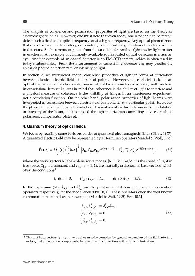
4. Quantum theory of optical fields

We begin by recalling some basic properties of quantized electromagnetic fields (Dirac, 1957).A quantized electric field may be represented by a Hermitian operator (Mandel & Wolf, 1995)

E(r, t) = i ∑k

∑s

(1

2hω

) 12 [

ak,sCk,sǫǫǫk,sei(k·r−ωt) − a†k,sC∗

k,sǫǫǫ∗k,se−i(k·r−ωt)

], (31)

where the wave vectors k labels plane wave modes, |k| = k = ω/c, c is the speed of light infree space, Ck,s is a constant, and ǫǫǫk,s (s = 1, 2), are mutually orthonormal base vectors, whichobey the conditions8

k · ǫǫǫk,s = 0, ǫǫǫ∗k,s · ǫǫǫk,s′ = δss′ , ǫǫǫk,1 × ǫǫǫk,2 = k/k. (32)

In the expansion (31), ak,s and a†k,s are the photon annihilation and the photon creation

operators respectively, for the mode labeled by (k, s). These operators obey the well knowncommutation relations [see, for example, (Mandel & Wolf, 1995), Sec. 10.3]

[ak,s, a†

k′ ,s′

]= δ3

kk′δss′ ,[ak,s, ak′ ,s′

]= 0, (33)

[a†

k,s, a†k′ ,s′

]= 0,

8 The unit base vectors ǫǫǫk1, ǫǫǫk2 may be chosen to be complex for general expansion of the field into twoorthogonal polarization components, for example, in connection with elliptic polarization.


www.intechopen.com



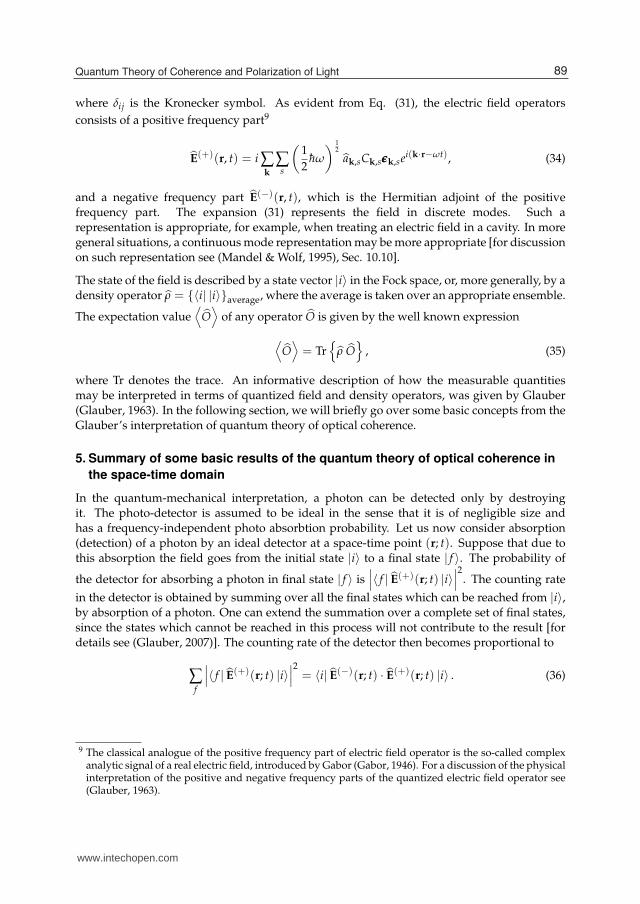
where δij is the Kronecker symbol. As evident from Eq. (31), the electric field operators

consists of a positive frequency part9

E(+)(r, t) = i ∑

k

∑s

(1

2hω

) 12

ak,sCk,sǫǫǫk,sei(k·r−ωt), (34)

and a negative frequency part E(−)(r, t), which is the Hermitian adjoint of the positivefrequency part. The expansion (31) represents the field in discrete modes. Such arepresentation is appropriate, for example, when treating an electric field in a cavity. In moregeneral situations, a continuous mode representation may be more appropriate [for discussionon such representation see (Mandel & Wolf, 1995), Sec. 10.10].

The state of the field is described by a state vector |i〉 in the Fock space, or, more generally, by adensity operator ρ = {〈i| |i〉}average, where the average is taken over an appropriate ensemble.

The expectation value⟨

O⟩

of any operator O is given by the well known expression

⟨O⟩= Tr

{ρ O

}, (35)

where Tr denotes the trace. An informative description of how the measurable quantitiesmay be interpreted in terms of quantized field and density operators, was given by Glauber(Glauber, 1963). In the following section, we will briefly go over some basic concepts from theGlauber’s interpretation of quantum theory of optical coherence.

5. Summary of some basic results of the quantum theory of optical coherence in

the space-time domain

In the quantum-mechanical interpretation, a photon can be detected only by destroyingit. The photo-detector is assumed to be ideal in the sense that it is of negligible size andhas a frequency-independent photo absorbtion probability. Let us now consider absorption(detection) of a photon by an ideal detector at a space-time point (r; t). Suppose that due tothis absorption the field goes from the initial state |i〉 to a final state | f 〉. The probability of

the detector for absorbing a photon in final state | f 〉 is∣∣∣〈 f | E(+)(r; t) |i〉

∣∣∣2. The counting rate

in the detector is obtained by summing over all the final states which can be reached from |i〉,by absorption of a photon. One can extend the summation over a complete set of final states,since the states which cannot be reached in this process will not contribute to the result [fordetails see (Glauber, 2007)]. The counting rate of the detector then becomes proportional to

∑f

∣∣∣〈 f | E(+)(r; t) |i〉

∣∣∣2= 〈i| E

(−)(r; t) · E(+)(r; t) |i〉 . (36)

9 The classical analogue of the positive frequency part of electric field operator is the so-called complexanalytic signal of a real electric field, introduced by Gabor (Gabor, 1946). For a discussion of the physicalinterpretation of the positive and negative frequency parts of the quantized electric field operator see(Glauber, 1963).


www.intechopen.com


If one considers the random fluctuations associated with light, one leads to a more generalexpression involving the density operator. The average counting rate of a photo-detectorplaced at a position r at time t then becomes proportional to [c.f (Glauber, 1963), Eq. (3.3)]

R(r, t) ≡ Tr{

ρ E(−)(r, t) · E

(+)(r, t)}

. (37)

Here the dot (·) denotes scalar product.

Using similar arguments, one can obtain quantum-mechanical analogues of all correlationfunctions (such as mutual coherence function etc.) used in the classical theory. The first-ordercorrelation properties (corresponds to second-order properties in the classical theory) of thefield may be specified by a 3 × 3 correlation matrix (Glauber, 1963)

←→G (1)(r, t; r

′, t′) ≡[

G(1)μν (r, t; r

′, t′)]

≡[Tr

{ρ E

(−)μ (r, t)E

(+)ν (r′, t′)

}], (38)

where μ, ν label, mutually orthogonal components of the electric field operator. For thesake of simplicity, let us neglect the polarization properties of the light, restricting our

analysis to scalar fields. Hence, with a suitable choice of axes, only one element G(1)μμ (r, t; r′, t′)

[no summation over repeated indices] of←→G (1)(r, t; r′, t′) will completely characterize all

first-order correlation properties of the field in the space-time domain. We omit the suffixμ and write

G(1)(r, t; r′, t′) = Tr

{ρ E(−)(r; t)E(+)(r′; t′)

}. (39)

The simplest coherence properties of light, in the space-time domain, are characterized by the

first-order correlation function←→G (1)(r, t; r′, t′). In terms of it one can define the first-order

degree of coherence by the formula [(Glauber, 1963), Eq. (4)]

g(1)(r, t; r′, t′) ≡

G(1)(r, t; r′, t′)√G(1)(r; t; r; t)

√G(1)(r′; t′; r′; t′)

. (40)

The modulus of g(1)(r, t; r′, t′) may be shown to be bounded by zero and unity [(Glauber,1963), Eq. (4.2)], i.e.,

0 ≤ |g(1)(r, t; r′, t′)| ≤ 1. (41)

It can be shown that this quantity is related to fringe visibility in interference experiments [see,for example, (Glauber, 2007), Sec. 2.7.2]. Complete first-order coherence (corresponding tosecond-order coherence in classical theory) is characterized by the condition |g(1)(r, t; r′, t′)| =1, and complete first-order incoherence by the other extreme, g(1)(r, t; r′, t′) = 0. Equations(8), and (40) may look similar, but one must appreciate the fact that the quantum mechanicalinterpretation is much more effective as one goes to a low-intensity domain, where absorptionor emission of one, or, few numbers of photons may affect the experimental observations.

Detailed descriptions on this topic have been discussed in many scholarly articles [see, forexample, (Glauber, 1963; 2007; Mandel & Wolf, 1995)].


www.intechopen.com



6. Quantum theory of optical coherence in space-frequency domain

In this section we present a quantum-mechanical theory of first-order optical coherence forstatistically non-stationary light in the space-frequency domain. We discuss some relevantcorrelation functions, associated with the quantized field and the density operator, which canbe introduced in the space-frequency representation. We also show, by use of the technique oflinear filtering, that these new correlation functions may be related to the photo-counting rateand to well known coherence-functions of space-time domain. We consider non-stationarylight10, because the assumption of statistical stationarity is not always appropriate, especiallyin many situations encountered in quantum optics where light emission may take place overa finite time-interval. A detailed description of the main material presented in this section hasbeen recently published (Lahiri & Wolf, 2010c).

6.1 Correlation functions in the space-frequency domain

Let us first note some properties of the operator e(r, ω), which is the Fourier transform ofE(r; t), i.e., which is given by

e(r, ω) =1

2π

∫ ∞

−∞E(r; t)eiωt dt. (42)

Using the fact that E(r; t) = E(+)(r; t) + E(−)(r; t), one may express e(r, ω) in the form

e(r, ω) = e(+)(r, ω) + e

(−)(r, ω), (43)

where

e(+)(r, ω) =

1

2π

∫ ∞

−∞E(+)(r; t)eiωt dt, (44a)

e(−)(r, ω) =

1

2π

∫ ∞

−∞E(−)(r; t)eiωt dt. (44b)

Using the property{

E(+)(r; t)}†

= E(−)(r; t), it follows from Eqs. (44) that{

e(+)(r, ω)}†

=

e(−)(r,−ω).

Let us now consider the following 3 × 3 correlation matrix

←→W

(1)(r, ω; r′, ω′) ≡

[W

(1)μν (r, ω; r

′, ω′)]≡ Tr

{ρ e

(−)μ (r,−ω)e

(+)ν (r′, ω′)

}. (45)

On using Eqs. (44) and (45), one can readily show that the elements of the correlation matrices←→G (1)(r, t; r′, t′) and

←→W (1)(r, ω; r′, ω′) are Fourier transforms of each other, i.e., that

W(1)

μν (r, ω; r′, ω′) =

(1

2π

)2 ∞�

−∞

G(1)μν (r, t; r

′, t′)ei(−ωt+ω′t′) dt dt′, (46a)

G(1)μν (r, t; r

′, t′) =∞�

0

W(1)

μν (r, ω; r′, ω′)ei(ωt−ω′t′) dω dω′. (46b)

10 Attempts to formulate coherence theory for classical non-stationary fields have been made (Bertolottiet al., 1995; Sereda et al., 1998).


www.intechopen.com


We will restrict our analysis to scalar fields. Therefore, the 3 × 3 correlation matrix←→W (1)(r, ω; r′, ω′) may now be replaced by the correlation function

W(1)(r, ω; r

′, ω′) = Tr{

ρ e(−)(r,−ω)e(+)(r′, ω′)}

, (47)

which, in analogy with the relations (46), is the Fourier transform of G(1)(r, t; r′, t′); viz,

W(1)(r, ω; r

′, ω′) =

(1

2π

)2 ∞�

−∞

G(1)(r, t; r′, t′)ei(−ωt+ω′t′) dt dt′, (48a)

G(1)(r, t; r′, t′) =

∞�

0

W(1)(r, ω; r

′, ω′)ei(ωt−ω′t′) dω dω′. (48b)

We will refer to W (1)(r, ω; r′, ω′) as the two-frequency cross-spectral density function (tobe abbreviated by two-frequency CSDF) and the single-frequency correlation functionW (1)(r, ω; r′, ω) as the cross-spectral density function (CSDF) of the field, in analogy withterminology used in the classical theory.

6.2 Physical interpretation of correlation functions in the space-frequency domain

Let us now assume that a light beam is transmitted by a linear filter which allows only anarrow frequency band to pass through it. Suppose that the light, emerging from the filter,has mean frequency ω and effective bandwidth Δω ≪ ω. The field operators representingthis filtered narrow-band light in the space-frequency domain, may then be represented bythe formulas

e(+)(ω)

(r, ω) = T(ω)(ω)e(+)(r, ω), (49a)

e(−)(ω)

(r,−ω) = T∗(ω)(ω)e(−)(r,−ω), (49b)

where T(ω)(ω) is the transmission function of the filter, whose modulus is negligible outsidethe pass-band ω − Δω/2 ≤ ω ≤ ω + Δω/2 of the filter. Using Eqs. (47) and (49), it followsthat for the filtered light,

W(1)(ω)

(r, ω; r′, ω′) = T∗

(ω)(ω)T(ω)(ω′)W (1)(r, ω; r

′, ω′). (50)

Here, the function W(1)(ω)

(r, ω; r′, ω′) is the two-frequency CSDF of the filtered light, of mean

frequency ω, and W (1)(r, ω; r′, ω′) on the right hand side is the two-frequency CSDF of theunfiltered light incident on the filter.

From Eqs. (48b) and (50), one readily finds that the space-time correlation function

G(1)(ω)

(r; t; r′; t′) of the filtered narrow-band light is given by the expression

G(1)(ω)

(r; t; r′; t′) =

ω+Δω/2�

ω−Δω/2

T∗(ω)(ω)T(ω)(ω

′)W (1)(r, ω; r′, ω′)ei(ωt−ω′t′) dω dω′. (51)


www.intechopen.com



Because of the assumption that Δω/ω ≪ 1, the function W (1)(r, ω; r′, ω′) in Eq. (51) does notchange appreciably as function of ω and ω′ over the ranges ω − Δω/2 ≤ ω ≤ ω + Δω/2,ω − Δω/2 ≤ ω′ ≤ ω + Δω/2 and is approximately equal to W (1)(r, ω; r′, ω). From Eq. (51) itthen follows that

G(1)(ω)

(r; t; r′; t′) ≈ W

(1)(r, ω; r′, ω)

ω+Δω/2�

ω−Δω/2


′)ei(ωt−ω′t′) dω dω′. (52)

6.3 Physical significance of W (1)(r, ω; r, ω)

Let us consider light generated by some physical process which begins at time t = 0 and ceasesat time t = T , say; for example light emitted by a collection of exited atoms. Clearly, suchlight is not statistically stationary. Suppose now that this light is filtered and is then incidenton a photo-detector. It follows from Eq. (52) that the average counting rate R(ω)(r; t) ≡

G(1)(ω)

(r; t; r; t) of the detector placed at a point r, at time t, is given by the expression

R(ω)(r; t) ≈ W(1)(r, ω; r, ω)

ω+Δω/2�

ω−Δω/2


′)ei(ω−ω′)t dω dω′. (53)

Since, R(ω)(r; t) = 0, unless 0 < t < T , the total energy E (r; ω) detected (total counts) by thephoto-detector will be proportional to

E (r; ω) ≡∫ T

0R(ω)(r; t) dt =

∫ ∞

−∞R(ω)(r; t) dt

≈ W(1)(r, ω; r, ω)

{2π

∫ ω+Δω/2

ω−Δω/2

∣∣∣T(ω)(ω)∣∣∣2

dω

}(54)

Thus, we may conclude that the total energy E (r; ω) detected by the photo-detector, placedat a point r in the path of a narrow-band light beam of mean frequency ω, is proportional toW (1)(r, ω; r, ω), i.e., that

E (r; ω) ≡∫ T

0R(ω)(r; t) dt ∝ W

(1)(r, ω; r, ω), (55)

the proportionality constant being dependent on the filter and on the choice of units. In otherwords, the correlation function W (1)(r, ω; r, ω) provides a measure of the energy density, at apoint r, associated with the frequency ω of light. It is evident that W (1)(r, ω; r, ω) ≥ 0.

W (1)(r, ω; r, ω) must not be confused with the well-known Wiener’s spectral density (Wiener,1930) of statistically stationary light. In the quantum mechanical interpretation, Wiener’sspectral density is equivalent to the counting rate of the photo-detector, associated with afrequency. On the other hand, the quantity W (1)(r, ω; r, ω) represents the total counts in thephoto-detector associated with the frequency ω. Therefore, W (1)(r, ω; r, ω) has a differentdimension than Wiener’s spectral density. Even in the stationary limit, W (1)(r, ω; r, ω) doesnot reduce to the Wiener’s spectral density. In fact, in such a case, the energy density E (r; ω)will be infinitely large and hence, in that limit, the quantity W (1)(r, ω; r, ω) will not be useful.


www.intechopen.com


For a light that is not statistically stationary, defining spectral density is a nontrivial problemwhich is still a subject of an active discussion. Many publications have been dedicated to itand several different definitions have been proposed [see, for example, (Eberly & Wódkievicz,1977; Lampard, 1954; Mark, 1970; Page, 1952; Ponomarenko et al., 2004; Silverman, 1957)].Nevertheless, for statistically non-stationary processes, W (1)(r, ω; r, ω) is measurable and aphysically meaningful quantity. In the following sections we show that it has an importantrole in defining the spectral-degree of coherence of non-stationary light.

6.4 First-order coherence

We will now consider the first-order coherence properties of non-stationary light, againrestricting ourselves to scalar fields. As in the previous Section, we will consider a filterednarrow-band light. On using Eqs. (40) and (52), one then has

g(1)(ω)

(r, t; r′, t′) ≈

W (1)(r, ω; r′, ω)√W (1)(r, ω; r, ω)

√W (1)(r′, ω; r′, ω)

Θ(t, t′), (56)

where

Θ(t, t′) =

� ω+Δω/2ω−Δω/2 T∗

(ω)(ω)T(ω)(ω′)ei(ωt−ω′t′) dω dω′

∣∣∣∫ ω+Δω/2

ω−Δω/2 T(ω)(ω)e−iωt dω∣∣∣∣∣∣∫ ω+Δω/2

ω−Δω/2 T(ω)(ω)e−iωt′ dω∣∣∣. (57)

Since, the numerator on the right hand side of Eq. (57) factorizes into a product of the twointegrals which appear in the denominator, it is evident that

|Θ(t, t′)| = 1, (58)

for all values of t and t′. From Eqs. (56) and (58), one readily finds that the modulus ofthe first-order “space-time” degree of coherence of the filtered narrow-band light of meanfrequency ω, is given by the formula

∣∣∣g(1)(ω)(r, t; r

′, t′)∣∣∣ ≈

∣∣∣∣∣∣W (1)(r, ω; r′, ω)√

W (1)(r, ω; r, ω)√

W (1)(r′, ω; r′, ω)

∣∣∣∣∣∣. (59)

The expression within the modulus signs on the right-hand side is the normalized CSDF atthe frequency ω.

It may be concluded from Eq. (59) that this normalized CSDF provides a measure of first-ordercoherence of the filtered light of mean frequency ω. Consequently, one may define thefirst-order spectral degree of coherence at frequency ω by the formula

η(1)(r, ω; r′, ω) ≡

W (1)(r, ω; r′, ω)√W (1)(r, ω; r, ω)

√W (1)(r′, ω; r′, ω)

. (60)

It can be immediately shown that (Lahiri & Wolf, 2010c)

0 ≤ |η(1)(r, ω; r′, ω)| ≤ 1. (61)


www.intechopen.com



When |η(1)(r, ω; r′, ω)| = 1, the light may be said to be completely coherent at the frequency ω,and when η(1)(r, ω; r′, ω) = 0, it may be said to be completely incoherent at that frequency. Westress, once again, that W (1)(r, ω; r′, ω) and η(1)(r, ω; r′, ω) being single-frequency quantities,provide measures of the ability of a particular frequency-component of the light to interfere.

We will now return to the two-frequency correlation function W (1)(r, ω; r′, ω′) given byformula (47). It characterizes correlations between different frequency components of light,i.e., the ability of two different frequency components to interfere. Interference of fields ofdifferent frequencies has generally not been considered in the literature, probably becauseit is not a commonly observed phenomenon. According to the classical theory, differentfrequency components of statistically stationary light do not interfere (see, for example, (Wolf,2007b), Sec. 2.5). For the sake of completeness, we will now show that this fact is also truein the non-classical domain. The proof is similar to that for classical fields. If one considerslight whose fluctuations are statistically stationary in the wide sense, i.e., if G(1)(r, t; r′, t′) =G(1)(r, r′; t′ − t) then, ignoring some mathematical subtleties, one finds from Eq. (48a) that thetwo-frequency CSDF W (1)(r, ω; r′, ω′) has the form

W(1)(r, ω; r

′, ω′) = f [r, r′; (ω + ω′)/2]δ(ω − ω′), (62)

where f is, in general, a complex function of its arguments and δ denotes the Dirac deltafunction. This formula shows that when ω = ω′, the two-frequency CSDF W (1)(r, ω; r′, ω′) =0, implying that different frequency components of statistically stationary light do notinterfere. However, for non-stationary random processes, this correlation function may havea non-zero value and, consequently, interference among different frequency components maytake place. One may define a normalized two-frequency correlation function

η(1)(r, ω; r′, ω′) =

W (1)(r, ω; r′, ω′)√W (1)(r, ω; r, ω)W (1)(r′, ω′; r′, ω′)

(63)

as a generalized first-order spectral degree of coherence for a pair of frequencies ω and ω′. Itcan also be shown that (Lahiri & Wolf, 2010c)

0 ≤ |η(1)(r, ω; r′, ω′)| ≤ 1. (64)

The extreme value |η(1)(r, ω; r′, ω′)| = 1, which corresponds to maximum possiblefringe visibility observed in interference experiments, represents complete coherence in thespace-frequency domain. The other extreme value, η(1)(r, ω; r′, ω′) = 0, implies that nointerference fringes will be present, i.e that there is complete incoherence between differentfrequency components.

7. Polarization properties of optical beams

In this section we will discuss the polarization properties of light. As is clear from previousdiscussions that a scalar treatment will no more be sufficient for his purpose, and we haveto consider the vector nature of the field. However, since, we will restrict our analysis tobeam-like optical fields, we will encounter 2 × 2 correlation matrices.


www.intechopen.com


We consider the canonical experiment depicted in Fig. 2. Suppose that a light beam,propagating along the positive z axis, passes through a compensator, followed by a polarizer(see Fig. 2). Light emerging from the polarizer is linearly polarized along some direction,

Fig. 2. Illustrating notation relating to the canonical polarization experiment.

which makes an angle θ, say, with the positive direction of a chosen x axis. We call θ thepolarizer angle. Effects of the compensator may be described by introducing phase delays αx

and αy in the x and the y components of the field operator E(+) respectively. Suppose nowthat a photodetector is placed behind the polarizer (see Fig. 2), which detects photons thatemerge from the polarizer. From Eq. (37), it follows that the counting rate Rθ,α(r; t) in thedetector will be given by the formula

Rθ,α(r; t) = Tr{

ρ E(−)θ,α (r; t)E

(+)θ,α (r; t)

}, (65)

whereE(±)θ,α = E

(±)x eiαx cos θ + E

(±)y eiαy sin θ. (66)

Using Eqs. (65) and (66), one readily finds that the average counting rate of the photo-detectoris given by the expression

Rθ,α(r; t) = G(1)xx (r, t; r, t) cos2 θ + G

(1)yy (r, t; r, t) sin2 θ

+ 2

√G(1)xx (r, t; r, t)

√G(1)yy (r, t; r, t) sin θ cos θ|g

(1)xy (r; t)| cos

[βxy(r; t)− α

], (67)

where α = αy − αx and

g(1)xy (r; t) ≡

G(1)xy (r, t; r, t)

√G(1)xx (r, t; r, t)

√G(1)yy (r, t; r, t)

≡ |g(1)xy (r; t)|eiβxy(r;t). (68)

It is important to note that only the “equal-point” (r1 = r2 ≡ r) and “equal-time” (t1 = t2 ≡ t)

correlation matrix←→G (1)(r, t; r, t) contributes to the photon counting rate. We will refer to this

matrix as the quantum polarization matrix. Equation (67) makes it possible to determine the

elements of the quantum polarization matrix←→G (1)(r, t; r, t) in a similar way as is done for the

elements of the analogous correlation matrix for a classical field, introduced in Ref. (Wolf,


www.intechopen.com



1959). One can readily show that

G(1)xx (r, t; r, t) =R0,0(r; t), (69a)

G(1)yy (r, t; r, t) =Rπ/2,0(r; t), (69b)

G(1)xy (r, t; r, t) =

1

2

[Rπ/4,0(r; t)−R3π/4,0(r; t)

]+

i

2

[Rπ/4,π/2(r; t)−R3π/4,π/2(r; t)

], (69c)

G(1)yx (r, t; r, t) =

1

2

[Rπ/4,0(r; t)−R3π/4,0(r; t)

]−

i

2

[Rπ/4,π/2(r; t)−R3π/4,π/2(r; t)

]. (69d)

Let us now briefly examine some properties of the quantum polarization matrix←→G (1)(r, t; r, t). Each element of this matrix, being a correlation function, has the properties

of a scalar product11. In particular, the elements of any such matrix satisfy the constraints

G(1)μμ (r, t; r, t) ≥ 0, (70a)

G(1)μν (r, t; r, t) =

{G(1)νμ (r, t; r, t)

}∗, (70b)

Det←→G (1)(r, t; r, t) ≥ 0, (70c)

where μ = x, y; ν = x, y and Det denotes the determinant. Conditions (70a) and (70c) implythat a quantum polarization matrix is always non-negative definite. Formula (70c) follows fromthe Cauchy-Schwarz inequality. From Eqs. (68) and (70c), it follows that

0 ≤ |g(1)xy (r; t)| ≤ 1. (71)

7.1 Unpolarized light beam

We will now assume that an unpolarized photon-beam12 is used in the experiment depicted inFig. 2. For such a beam, the photon detection rate Rθ,α(r; t), has to be independent of θ and α

and consequently, one has from Eq. (67) that

g(1)xy (r; t) = 0, (72a)

and G(1)xx (r, t; r, t) = G

(1)yy (r, t; r, t) ≡ A(r; t), say, (72b)

where A(r; t) is a real function of space and time and A(r; t) ≥ 0. From Eqs. (72) it is evident

that for an unpolarized beam, the quantum polarization matrix←→G

(1)(u)

(r; t; r; t) is proportional

to a unit matrix, i.e., that←→G

(1)(u)

(r; t; r; t) = A(r; t)

(1 00 1

). (73)

11 The proof is similar to that given for scalar field operators (Titulaer & Glauber, 1965).12 For discussion on unpolarized radiation see, for example, Refs. (Agarwal, 1971; Prakash et al., 1971)


www.intechopen.com


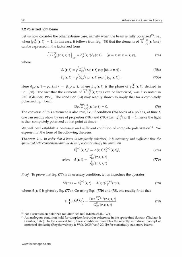
7.2 Polarized light beam

Let us now consider the other extreme case, namely when the beam is fully polarized13, i.e.,

when |g(1)xy (r; t)| = 1. In this case, it follows from Eq. (68) that the elements of

←→G

(1)(p)

(r; t; r; t)

can be expressed in the factorized form

{←→G

(1)(p)

(r; t; r; t)}

μν= E∗

μ (r; t)Eν(r; t), (μ = x, y; ν = x, y), (74)

where

Ex(r; t) =

√G(1)xx (r, t; r, t) exp [iφxx(r; t)] , (75a)

Ey(r; t) =

√G(1)yy (r, t; r, t) exp

[iφyy(r; t)

]. (75b)

Here φyy(r; t) − φxx(r; t) = βxy(r; t), where βxy(r; t) is the phase of g(1)xy (r; t), defined in

Eq. (68). The fact that the elements of←→G

(1)(p)

(r; t; r; t) can be factorized, was also noted in

Ref. (Glauber, 1963). The condition (74) may readily shown to imply that for a completelypolarized light beam

Det←→G

(1)(p)

(r; t; r; t) = 0. (76)

The converse of this statement is also true, i.e., if condition (76) holds at a point r, at time t,

one can readily show by use of properties (70a) and (70b) that |g(1)xy (r; t)| = 1; hence the light

is then completely polarized at that point at time t.

We will next establish a necessary and sufficient condition of complete polarization14. Weexpress it in the form of the following theorem:

Theorem 7.1. In order that a beam is completely polarized, it is necessary and sufficient that thequantized field components and the density operator satisfy the condition

E(+)x (r; t)ρ = A(r; t)E

(+)y (r; t)ρ, (77a)

where A(r; t) =G(1)yx (r, t; r, t)

G(1)yy (r, t; r, t)

, (77b)

Proof. To prove that Eq. (77) is a necessary condition, let us introduce the operator

M(r; t) = E(+)x (r; t)− A(r; t)E

(+)y (r; t), (78)

where A(r; t) is given by Eq. (77b). On using Eqs. (77b) and (78), one readily finds that

Tr{

ρ M† M}=

Det←→G (1)(r, t; r, t)

G(1)yy (r, t; r, t)

. (79)

13 For discussion on polarized radiation see Ref. (Mehta et al., 1974)14 An analogous condition hold for complete first-order coherence in the space-time domain (Titulaer &

Glauber, 1965). In the classical limit, these conditions resembles the recently introduced concept ofstatistical similarity (Roychowdhury & Wolf, 2005; Wolf, 2010b) for statistically stationary beams.


www.intechopen.com



If the field is completely polarized, Eqs. (76) and (79) imply that

Tr{

ρ M† M}= 0, (80)

and, consequently,Mρ = ρM† = 0. (81)

Substituting for M from Eq. (78) into Eq. (81), one readily find that condition (77) is satisfied.Thus we have proved that Eq. (77) is a necessary condition for complete polarization of a lightbeam at a point r, at time t.

On the other hand, if one imposes condition (77) on the components of the field operator and

evaluates Det←→G

(1)(p)

(r; t; r; t), one readily obtains Eq. (76), i.e., one finds that if condition (77)

holds, the beam is completely polarized. Hence this condition is also a sufficiency condition.

7.3 Partially polarized light beam

We have discussed the properties of completely polarized and completely unpolarized beams.

Next we consider beams which are partially polarized, i.e., beams for which 0 < |g(1)xy (r; t)| <

1.

We will first establish the following result: If a beam of partially polarized photons is incident on aphoto-detector, the average counting rate of the detector, at any time t, can always be decomposed intotwo parts, one which represents the counting rate for a polarized beam and the other the counting rate

for an unpolarized beam. It can be proved that any quantum polarization matrix←→G (1)(r, t; r, t)

can be uniquely decomposed in the form (Lahiri & Wolf, 2010b)

←→G (1)(r, t; r, t) =

←→G

(1)(p)

(r; t; r; t) +←→G

(1)(u)

(r; t; r; t), (82)

where the elements of←→G

(1)(p)

(r; t; r; t) and←→G

(1)(u)

(r; t; r; t) can be uniquely expressed in terms

of the elements of←→G (1)(r, t; r, t). From Eqs. (37) and (82), one can at once deduce that the

counting rate of the photo-detector has contribution from an unpolarized part and from apolarized part; i.e., that

R(r, t) = Tr←→G (1)(r, t; r, t) = R(p)(r, t) +R(u)(r, t). (83)

By analogy with the classical theory of stochastic electromagnetic beams, we define the degreeof polarization P , at a point P(r), at time t, as the ratio of the photon counting rate for thepolarized part to the total counting rate:

P(r; t) ≡R(p)(r, t)

R(r, t)=

Tr←→G

(1)(p)

(r; t; r; t)

Tr←→G (1)(r, t; r, t)

. (84)


www.intechopen.com


On expressing the elements of←→G

(1)(p)

(r; t; r; t) in terms of the elements of←→G (1)(r, t; r, t), one

can show that (Lahiri & Wolf, 2010b)

P(r; t) =

√√√√√1 −4 Det

←→G (1)(r, t; r, t)

{Tr←→G (1)(r, t; r, t)

}2. (85)

From Eqs. (73) and (85), one can readily show that for a beam of unpolarized photons P = 0;and from Eqs. (82) and (85) it follows, at once, that for a completely polarized beam of photonsP(r; t) = 1.

Although, formulas (28), and (85) look similar in form, one must bear in mind that thedefinition used in classical theory is not appropriate for light of low intensity, nor has it beenshown that it is valid for fields that are not necessarily statistically stationary. On the otherhand, the expression (85) for the degree of polarization applies also to low intensity light andfor light whose statistical properties are characterized by non-stationary ensembles, such as,for example, fields associated with a non-stationary ensemble of pulses.

8. Wave-particle duality, partial coherence and partial polarization of light

Quantum systems (quantons15) possess properties of both particles and waves. Bohr’scomplementarity principle (Bohr, 1928) suggests that these two properties are mutuallyexclusive. In other words, depending on the experimental situation, a quanton will behaveas a particle or as a wave. In the third volume of his famous lecture series (Feynman et al.,1966), Feynman emphasized that this wave-particle duality may be understood from Young’stwo-pinhole interference experiments (Young, 1802). In such an experiment, a quantonmay arrive at the detector along two different paths. If one can determine which path thequanton traveled, then no interference fringe will be found (i.e., the quanton will showcomplete particle behavior). On the other hand, if one cannot obtain any information about thequanton’s path, then interference fringes, with unit visibility, will be obtained (i.e., the quantonwill show complete wave behavior), assuming that the intensities at the two pinholes are thesame. In the intermediate case when one has partial “which-path information” (WPI), fringeswith visibility smaller than unity are obtained, even if the intensities at the two pinholesare equal. For the sake of brevity, we will use the term “best circumstances” to refer to thesituation when in an Young’s interference experiment, the intensities at the two pinholes areequal, or to equivalent situations in other interferometric setups.

The relation between fringe visibility (degree of coherence) and WPI has been investigated byresearchers [see, for example, (Englert, 1996; Jaeger et al., 1995; Mandel, 1991)]. It has beenestablished that a quantitative measure of WPI and fringe-visibility obey a certain inequality.In this section, we will first recollect the results obtained by Mandel and then will show thatit is not only the fringe-visibility, but also the polarization properties of the superposed light,which may depend on WPI in an interference experiment.

15 This abbreviation is due to M. Bunge [see, for example, J.-M. Lévy-Leblond, Physica B 151, 314 (1988)].


www.intechopen.com



Suppose, that |ψ1〉 and |ψ2〉 represent two normalized single-photon states (eigenstates of thenumber operator), so that

〈ψ1|ψ2〉 = 〈ψ2|ψ1〉 = 0, (86a)

〈ψ1|ψ1〉 = 〈ψ2|ψ2〉 = 1. (86b)

We will consider the superposition of the two states in some interferometric arrangement,where a photon may travel along two different paths. Suppose that |ψID〉 represents a state oflight, which is formed by coherent superposition of the two states |ψ1〉 and |ψ2〉, i.e., that

|ψID〉 = α1 |ψ1〉+ α2 |ψ1〉 , |α1|2 + |α2|

2 = 1, (87)

where α1 and α2 are, in general, two complex numbers. In this case, a photon may be inthe state |ψ1〉 with probability |α1|

2, or in the state |ψ2〉 with probability |α2|2, but the two

possibilities are intrinsically indistinguishable. The density operator ρID will then have theform

ρID = |α1|2 |ψ1〉〈ψ1|+ |α2|

2 |ψ2〉〈ψ2|+ α∗1α2 |ψ2〉〈ψ1|+ α∗2α1 |ψ1〉〈ψ2| . (88)

In the other extreme case, when the state of light is due to incoherent superposition of the twostates, the density operator ρD will be given by the expression

ρD = |α1|2 |ψ1〉〈ψ1|+ |α2|

2 |ψ2〉〈ψ2| . (89)

Here |α1|2 and |α2|

2 again represent the probabilities that the photon will be in state |ψ1〉 orin state |ψ2〉, but now the two possibilities are intrinsically distinguishable. Mandel (Mandel,1991) showed that in any intermediate case, the density operator

ρ = ρ11 |ψ1〉〈ψ1|+ ρ12 |ψ1〉〈ψ2|+ ρ21 |ψ2〉〈ψ1|+ ρ22 |ψ2〉〈ψ2| (90)

can be uniquely expressed in the form

ρ = I ρID + (1 −I )ρD, 0 ≤ I ≤ 1. (91)

Mandel defined I as the degree of indistinguishability. If I = 0, the two paths arecompletely distinguishable, i.e., one has complete WPI; and if I = 1, they are completelyindistinguishable, i.e., one has no WPI. In the intermediate case 0 < I < 1, the twopossibilities may be said to be partially distinguishable. Clearly, I may be considered asa measure of WPI. According to Eqs. (90) and (91), one can always express ρ in the form

ρ = |α1|2 |ψ1〉〈ψ1|+ |α2|

2 |ψ2〉〈ψ2|+I (α∗1α2 |ψ2〉〈ψ1|+ α∗2α1 |ψ1〉〈ψ2|). (92)

Clearly, the condition of “best circumstances” requires that |α1| = |α2|.

8.1 WPI and partial coherence

Mandel considered a Young’s interference experiment, in which the two pinholes (secondarysources) were labeled by 1 and 2. He assumed |n〉j to be a state representing n photonsoriginated from pinhole j (n = 0, 1; j = 1, 2). Clearly, in this case

|ψ1〉 = |1〉1 |0〉2 , |ψ2〉 = |0〉1 |1〉2 . (93)


www.intechopen.com


Calculations show that [for details see (Mandel, 1991)] “visibility ≤ I ”, and the equalityholds in the special case when |α1| = |α2|. Since fringe-visibility is a measure of coherenceproperties of light (modulus of degree of coherence is equal to the fringe visibility), Mandel’sresult displays an intimate relationship between wave-particle duality and partial coherence.

8.2 WPI and partial polarization

Let us now assume that |ψ1〉 and |ψ2〉 are of the form

|ψ1〉 = |1〉x |0〉y , (94a)

|ψ2〉 = |0〉x |1〉y , (94b)

where the two states are labeled by the same (vector) mode k, and x, y are two mutuallyorthogonal directions, both perpendicular to the direction of k. For the sake of brevity, k isnot displayed in Eqs. (94). Clearly |ψ1〉 represents the state of a photon polarized along the xdirection, and |ψ2〉 represents that along the y direction. In the present case, one may express

E(+)i (r; t) in the form

E(+)i (r; t) = Cei(k·r−ωt) ai, (i = x, y), (95)

where the operator ai represents annihilation of a photon in mode k, polarized along the i−axis, and C is a constant. From Eqs. (38), (92), and (95), one readily finds that the quantum

polarization matrix←→G (1)(r, t; r, t) has the form

←→G (1)(r, t; r, t) = |C|2

(|α1|

2 I α∗1α2

I α1α∗2 |α2|2

). (96)

From Eqs. (84) and (96) and using the fact |α1|2 + |α2|

2 = 1, one finds that, in this case, thedegree of polarization is given by the expression

P =√(|α1|2 − |α2|2)2 + 4|α1|2|α2|2I 2. (97)

It follows from Eq. (97) by simple calculations that

P2 −I

2 = (1 −I2)(2|α1|

2 − 1)2. (98)

Using the fact that 0 ≤ I ≤ 1, one readily finds that

P ≥ I . (99)

Thus, the degree of polarization of the out-put light in a single-photon interference experimentis always greater or equal to the degree of indistinguishability (I ) which a measure of“which-path information”.

Let us now assume that the condition of “best circumstances” holds, i.e., one has |α1| = |α2|.It then readily follows from Eq. (97) that

P = I . (100)


www.intechopen.com



This formula shows that under the “best circumstances”, the degree of indistinguishability (ameasure of WPI) and the degree of polarization are equal. The physical interpretation of thisresult may be understood from the following consideration: If one has complete “which-pathinformation” (i.e., I = 0), then it follows from Eq. (100) that the degree of polarization of thelight emerging from the interferometer is equal to zero. Complete “which-path information”in an single-photon interference experiment implies that a photon shows complete particlenature, and our analysis suggests that in such a case light is completely unpolarized. In theother extreme case, when one has no “which-path information”, i.e., when a photon does notdisplay any particle behavior, the output light will be completely polarized. Any intermediatecase will produce partially polarized light. For details analysis see (Lahiri, 2011).

9. Conclusions

We conclude this chapter by saying that we have given a description of first-order coherenceand polarization properties of light. The main aim of this chapter was to emphasize the factthat although, coherence and polarization seem to be two different optical phenomena, both ofthem can be described by analogous theoretical techniques. Our discussion also emphasizessome newly obtained results in quantum theory of optical coherence in the space-frequencydomain, and in quantum theory of polarization of light beams.

10. Acknowledgements

The author sincerely thanks Professor Emil Wolf for many helpful discussions and insightfulcomments. This research was supported by the US Air Force Office of Scientific Researchunder grant No. FA9550-08-1-0417.

11. References

Agarwal, G. S. (1971). On the state of unpolarized radiation, Lett. Al Nuovo Cimento 1.Arago, F. & Fresnel, A. (1819). L’action queles rayons de lumiere polarisee exercent les uns sur

les autres, Ann. Chim. Phys. 2.Berek, M. (1926a). Z. Phys. 36.Berek, M. (1926b). Z. Phys. 36.Berek, M. (1926c). Z. Phys. 37.Berek, M. (1926d). Z. Phys. 40.Berry, H. G., Gabrielse, G. & Livingston, A. E. (1977). Measurement of the stokes parameters

of light, App. Opt. 16.Bertolotti, M., Ferrari, A. & Sereda, L. (1995). Coherence properties of nonstationary

polychromatic light sources, J. Opt. Soc. Am. B 12.Bohr, N. (1928). Das quantenpostulat und die neuere entwicklung der atomistik,

Naturwissenschaften 16.Born, M. & Wolf, E. (1999). Principles of Optics, (Cambridge University Press, Cambridge, 7th

Ed.).Brosseau, C. (1995). Fundamentals of Polarized Light: A Statistical Optics Approach, (Wiley).Brosseau, C. (2010). Polarization and coherence optics: Historical perspective, status, and

future directions, Prog. Opt. 54.Collett, E. (1993). Polarized light : fundamentals and applications, (New York, Marcel Dekker).


www.intechopen.com


Dirac, P. A. M. (1957). The Priciples of Quantum Mechanics, 4th Ed., Oxford University Press,Oxford, England.

Eberly, J. H. & Wódkievicz, K. (1977). The time dependent physical spectrum of light, J. Opt.Soc. Am. 67.

Englert, B.-G. (1996). Fringe vsibility and which-way information: an inequality, Phys. Rev.Lett. 77.

Feynman, R. P., Leighton, R. B. & Sands, M. (1966). The Feynman Lectures on Physics, Vol. III,Addison-Wesley Publishing Company, New York, USA.

Feynman, R. P., Leighton, R. & (Editor), E. H. (1985). Surely you’re joking Mr. Feynman!, (W. W.Norton & Company, New York).

Friberg, A. T. & Wolf, E. (1995). Relationships between the complex degrees of coherence inthe space-time and in the space-frequency domains, Opt. Lett. 20.

Gabor, D. (1946). Theory of communication, J. Inst. Elec. Eng. (London), Pt. III 93.Gabor, D. (1955). Light and information, Proceedings of a Symposium on Astronomical Optics and

Related Subjects, Edited by Zdenek Kopal .Glauber, R. J. (1963). The quantum theory of optical coherence, Phys. Rev. 130.Glauber, R. J. (2007). Quantum Theory of Optical Coherence (selected papers and lectures),

(Weinheim, WILEY-VCH Verlag Gmbh & Co. KGaA).Hooke, R. (1665). Micrographia: Or Some Physiological Descriptions of Minute Bodies Made

by Magnifying Glasses with Observations and Inquities thereupon, Martyn and Alleftry,Printers to the Royal Society, London, England.

Huygens, C. (1690). Traité de la lumière.Jackson, J. D. (2004). Classical electrodynamics, (John Wiley, New York, 3rd Ed.).Jaeger, G., Shimony, A. & Vaidman, L. (1995). Two interferometric complementarities, Phys.

Rev. A 51.James, D. F. V. (1994). Change in polarization of light beams on propagation in free space, J.

Opt. Soc. Am. A 11.Karczewski, B. (1963). Coherence theory of the electromagnetic field, Nuovo Cimento 30.Lahiri, M. (2009). Polarization properties of stochastic light beams in the spaceUtime and

spaceUfrequency domains, Opt. Lett. 34.Lahiri, M. (2011). Wave-particle duality and partial polarization of light in single-photon

interference experiments, Phys. Rev. A 83.Lahiri, M. & Wolf, E. (2009). Cross-spectral density matrices of polarized light beams, Opt.

Lett. 34.Lahiri, M. & Wolf, E. (2010a). Does a light beam of very narrow bandwidth always behave as

a monochromatic beam?, Phys. Lett. A 374.Lahiri, M. & Wolf, E. (2010b). Quantum analysis of polarization properties of optical beams,

Phys. Rev. A 82.Lahiri, M. & Wolf, E. (2010c). Quantum theory of optical coherence of non-stationary light in

the space-frequency domain, Phys. Rev. A 82.Lahiri, M. & Wolf, E. (2010d). Relationship between complete coherence in the space-time and

in the space-frequency domains, Phys. Rev. Lett. 105.Lahiri, M., Wolf, E., Fischer, D. G. & Shirai, T. (2009). Determination of correlation functions of

scattering potentials of stochastic media from scattering experiments, Phys. Rev. Lett.102.


www.intechopen.com



Lampard, D. G. (1954). Generalization of the wiener-khintchine theorem to nonstationaryprocesses, J. Appl. Phys. 25.

Laue, M. V. (1906). Zur thermodynamik der interferenezerscheinungen, Ann. d. Physik 20.Laue, M. V. (1907). Ann. d. Physik 23.Mandel, L. (1991). Coherence and indistinguishability, Opt. Lett. 16.Mandel, L. & Wolf, E. (1995). Optical Coherence and Quantum Optics, (Cambridge University

Press, Cambridge).Mark, W. D. (1970). Spectral analysis of the convolution and filtering of non-stationary

stochastic processes, J. Sound Vib. 11.Mehta, C. L. & Sharma, M.K. (1974). Diagonal coherent–state representation for polarized

light, Phys. Rev. A. 10.Michelson, A. A. (1890). Etude sur la constitution de la lumiere non polarisée et de la lumiere

partiellement polarisée, Phil. Mag. 30.Michelson, A. A. (1891a). Phil. Mag. 31.Michelson, A. A. (1891b). Phil. Mag. 31.Michelson, A. A. (1902). Light Waves and Their Uses, The University of Chicago Press, Chicago,

USA.Michelson, A. A. (1927). Studies in Optics, The University of Chicago Press, Chicago, USA.Mujat, M., Dogariu, A. & Wolf, E. (2004). A law of interference of electromagnetic beams of

any state of coherence and polarization and the fresnel–arago interference laws, J.Opt. Soc. Am. A. 21.

Page, C. H. (1952). Instantaneous power spectra, J. Appl. Phys. 23.Poincaré, H. (1892). Théorie Mathématique de la Lumiére, Vol 2, Georges Carré, Paris, France.Ponomarenko, S. A., Agrawal, G. P. & Wolf, E. (2004). Energy spectrum of a nonstationary

ensemble of pulses, Opt. Lett. 29.Prakash, H. & Chandra, N. (1971). Density operator of unpolarized radiation, Phys. Rev. A 4.Roychowdhury, H. & Wolf, E. (2005). Statistical similarity and the physical significance of

complete spatial coherence and complete polarization of random electromagneticbeams, Opt. Commun. 248.

Sereda, L., Bertolotti, M. & Ferrari, A. (1998). Coherence properties of nonstationary lightwave fields, J. Opt. Soc. Am. A 15.

Setälä, T., Nunziata, F. & Friberg, A. T. (2009). Differences between partial polarizations in thespaceUtime and spaceUfrequency domains, Opt. Lett. 34.

Silverman, R. A. (1957). Locally stationary random processes, Proc. I.R.E. (Trans. Inf. Th.) 3.Stokes, G. G. (1852). On the composition and resolution of streams of polarized light from

different sources, Trans. Cambr. Phil. Soc. 9.Titulaer, U. M. & Glauber, R. J. (1965). Correlation functions for coherent fields, Phys. Rev. 140.van Cittert, P. H. (1934). Physica 1.van Cittert, P. H. (1939). Physica 6.Verdet, E. (1865). Etude sur la constitution de la lumiere non polarisée et de la lumiere

partiellement polarisée, Annales scientifiques de l’E.N.S. 2.Wiener, N. (1927). Coherency matrices and quantum theory, J. Math. Phys. (M.I.T.) 7.Wiener, N. (1930). Generalized harmonic analysis, Acta Math. 55.Wiener, N. (1966). Generalized harmonic analysis and Tauberian theorems, (The M.I.T. Press).Wolf, E. (1954). Optics in terms of observable quantities, Nuovo Cimento 12.


www.intechopen.com


Wolf, E. (1955). A macroscopic theory of interference and diffraction of light from finite sourcesii. fields with a spectral range of arbitrary width, Proc. Roy. Soc. (London) A 230.

Wolf, E. (1959). Coherence properties of partially polarized electromagnetic radiation, NuovoCimento 13.

Wolf, E. (1981). New spectral representation of random sources and of the partially coherentfields that they generate, Opt. Commun. 38.

Wolf, E. (1982). New theory of partial coherence in the space-frequency domain. part i: spectraand cross spectra of steady-state sources, J. Opt. Soc. Am. 72.

Wolf, E. (1983). Young’s interference fringes with narrow-band light, Opt. Lett. 8.Wolf, E. (1986). New theory of partial coherence in the space-frequency domain. part ii:

Steady-state fields and higher-order correlations, J. Opt. Soc. Am. A 3.Wolf, E. (1987). Non-cosmological redshifts of spectral lines, Nature 326.Wolf, E. (2003a). Correlation-induced changes in the degree of polarization, the degree of

coherence, and the spectrum of random electromagnetic beams on propagation, Opt.Lett. 28.

Wolf, E. (2003b). Unified theory of coherence and polarization of random electromagneticbeams, Phys. Lett. A 312.

Wolf, E. (2007a). The influence of young’s interference experiment on the development ofstatistical optics, Progress in Optics 50.

Wolf, E. (2007b). Introduction to the Theory of Coherence and Polarization of Light, (CambridgeUniversity Press, Cambridge, 7th Ed.).

Wolf, E. (2009a). Solution to the phase problem in the theory of structure determination ofcrystals from x-ray diffraction experiments, Phys. Rev. Lett. 103.

Wolf, E. (2009b). Statistical similarity as a unifying concept in the theory of coherenceand polarization of light, Presented by M. Lahiri at the Koli Workshop on PartialElectromagnetic Coherence and 3D Polarization, Koli, Finland .

Wolf, E. (2010a). Determination of phases of diffracted x-ray beams in investigations ofstructure of crystals, Phys. Lett. A 374.

Wolf, E. (2010b). Statistical similarity as a unifying concept of the theories of coherence andpolarization of light, Opt. Commun. 283.

Wolf, E. (2011). History and solution of the phase problem in the theory of structuredetermination of crystals from x-ray diffraction measurements, Adv. Imag. Elec. Phys.165.

Young, T. (1802). An account of some cases of the production of colours, not hithertodescribed, Phil. Trans. Roy. Soc. Lond. 92.

Zernike, F. (1938). The concept of degree of cohernence and its application and its applicationto optical problems, Physica 5.


www.intechopen.com

Advances in Quantum TheoryEdited by Prof. Ion Cotaescu

ISBN 978-953-51-0087-4Hard cover, 248 pagesPublisher InTechPublished online 15, February, 2012Published in print edition February, 2012

InTech EuropeUniversity Campus STeP Ri Slavka Krautzeka 83/A 51000 Rijeka, Croatia Phone: +385 (51) 770 447 Fax: +385 (51) 686 166www.intechopen.com

InTech ChinaUnit 405, Office Block, Hotel Equatorial Shanghai No.65, Yan An Road (West), Shanghai, 200040, China

Phone: +86-21-62489820 Fax: +86-21-62489821

The quantum theory is the first theoretical approach that helps one to successfully understand the atomic andsub-atomic worlds which are too far from the cognition based on the common intuition or the experience of thedaily-life. This is a very coherent theory in which a good system of hypotheses and appropriate mathematicalmethods allow one to describe exactly the dynamics of the quantum systems whose measurements aresystematically affected by objective uncertainties. Thanks to the quantum theory we are able now to use andcontrol new quantum devices and technologies in quantum optics and lasers, quantum electronics andquantum computing or in the modern field of nano-technologies.

How to referenceIn order to correctly reference this scholarly work, feel free to copy and paste the following:

Mayukh Lahiri (2012). Quantum Theory of Coherence and Polarization of Light, Advances in Quantum Theory,Prof. Ion Cotaescu (Ed.), ISBN: 978-953-51-0087-4, InTech, Available from:http://www.intechopen.com/books/advances-in-quantum-theory/quantum-theories-of-coherence-and-polarization-of-light

© 2012 The Author(s). Licensee IntechOpen. This is an open access articledistributed under the terms of the Creative Commons Attribution 3.0License, which permits unrestricted use, distribution, and reproduction inany medium, provided the original work is properly cited.

http://creativecommons.org/licenses/by/3.0

quantum theory of coherence and polarization of light

Documents