quarterly projection model for croatia - hnb
TRANSCRIPT

Quarterly Projection Model for Croatia
Nikola Bokan, Rafael Ravnik
Zagreb, September 2018
Surveys S-34


SURVEYS S-34

PUBLISHERCroatian National Bank Publishing Department Trg hrvatskih velikana 3, 10000 Zagreb Phone: +385 1 45 64 555 Contact phone: +385 1 45 65 006 Fax: +385 1 45 64 687
WEBSITEwww.hnb.hr
EDITOR-IN-CHIEFLjubinko Jankov
EDITORIAL BOARDVedran Šošić Gordi Sušić Davor Kunovac Tomislav Ridzak Evan Kraft Maroje Lang Ante Žigman
EDITORRomana Sinković
DESIGNERVjekoslav Gjergja
TECHNICAL EDITORSlavko Križnjak
The views expressed in this paper are not necessarily the views of the Croatian National Bank.Those using data from this publication are requested to cite the source.Any additional corrections that might be required will be made in the website version.
ISSN 1334-0131 (online)

Zagreb, September 2018
SURVEYS S-34
Quarterly Projection Model for Croatia
Nikola Bokan, Rafael Ravnik


ABSTRACT V
Quarterly Projection Model for Croatia
Abstract
This paper provides the documentation for a Quarterly Pro-jection Model (QPM) used in regular forecasting exercises in the Croatian National Bank. The proposed model is a reduced-form representation of an Open Economy New Keynesian gen-eral equilibrium model, expanded with some ad hoc features in order to capture empirical evidence about the Croatian econo-my. Special attention is paid to open economy features of the model, financial stability issues related to the high degree of credit euroization and monetary policy modeling. The main contribution to the existing literature is the monetary policy rule, which is represented by an exchange rate reaction func-tion with a slow-moving exchange rate target. The simulation and forecasting exercises conducted in this paper show that the model is able to produce precise forecasts of the main macro-economic variables and to explain important relationships and the transmission mechanisms of the Croatian economy.
Keywords: projection model, unconventional monetary policy rule,
nominal exchange rate, euroization
JEL: E37, E47, E52, F33, F41, H68
The authors would like to thank colleagues from OG Research for their support in the development of an earlier version of this model.

Abstract v
1 Introduction 1
2 The model 32.1 Main features of the model and some empirical
facts about the nominal exchange rate 32.2 Model equations 6
3 Calibration 143.1 Calibration of steady-state values 143.2 Calibration of business-cycle parameters 15
4 Forecasting 164.1 Baseline forecast 174.2 Conditional forecast 174.3 Using the QPM for forecasting exercises in the
Croatian National Bank 18
5 Model properties 185.1 Impulse response functions 185.2 Forecasting performance and goodness-of-fit 22
6 Concluding remarks 24
7 References 25
8 Appendix: List of variables 27
9 Appendix: List of equations 29
10 Appendix: Calibration 33
11 Appendix: Figures and tables 35
Contents

1 INTRODUCTION
Quarterly Projection Model for Croatia
1
1 Introduction
During the last decade, most central banks have developed so-called quarterly projection models (QPM) used for policy analysis and the forecasting of the main macroeconomic variables. Most of these models are best described as reduced form representations of structural New Keynesian general equilibrium models ex-panded with some ad hoc features. Although they lack explicit micro foundations and, thus, the strict theoreti-cal coherence of DSGE models, they are far more flexible from the modeling point of view and usually more successful in capturing and replicating the main characteristics of the modeled economy. The core structure of these QPMs is usually based on four standard behavioral equations: Phillips curve, IS curve, UIP relation and the monetary policy rule. Nevertheless, they can be extended to account for fiscal policy issues, real-financial linkages or labor market variables among other things. All real variables in this type of models are expressed as deviations from their long-run trends, therefore the term gap models is commonly used.1
In this paper we present a medium-scale gap model for the Croatian economy that contains most of the necessary features needed to describe the dynamics of a small open and euroized economy with an unconven-tional monetary policy rule. Whereas the core equations closely follow the basic structure of open economy New-Keynesian models, we have modified and added some equations in order to capture stylized facts and empirical evidence about the Croatian economy.2 Given the nonstandard nature of Croatian National Bank (CNB) monetary policy, particular attention was paid to the specification of the monetary rule. Instead of a standard interest rate Taylor rule, we specify monetary policy through an exchange rate rule and instead of ex-plicitly targeting inflation, the monetary authority in our model sets a moving nominal exchange rate target.3 Consequently, the main policy instrument is not the interest rate but the nominal euro vis-a-vis Croatian kuna exchange rate.4 Therefore, the monetary policymaker reacts to deviations of the nominal exchange rate from its targeted level, and the exchange rate is therefore kept smooth, as is observed in the data. It is important to note that the target level is allowed to drift, which means that it is not fixed at some predefined level. Moreover, not only exchange rate deviations, but also deviations of inflation from its implicit target enter into the reaction function. The described definition of the reaction function is a consequence of the CNB’s policy and its main objective (maintaining price stability). In order to achieve its final objective, the monetary policy maker sets an intermediate target (intermediate objective) which is managing the nominal exchange rate against the euro. By
1 For a short introduction about this type of gap model see Berg et al (2006).
2 The model presented here has some similarities with McCallum (2006) for Singapore, Pongsaparn (2007) for Thailand, OG Research (2011) for the Czech Republic, Salas (2010) for Peru and the models described in Benes et al (2003 and 2008).
3 More about managing exchange rates and monetary policy rules for small open economies can found in Ball (1998), Moron, and Winkelried (2005) and Benes et al (2011).
4 The CNB is using additional instruments as for instance open market operations, reserve requirement ratios and others. We will refrain from using these policy instruments in this paper since it is not possible to implement them all in a single model.

1 INTRODUCTION
Nikola Bokan, Rafael Ravnik
2
managing this exchange rate the CNB anchors inflation expectations. Such a monetary policy framework is a consequence of the high share of loans and deposits denominated in euro. Due to the mentioned deposit and credit euroization the Croatian economy is vulnerable to exchange rate shocks through the so-called balance sheet effect, which presents the main constraint for the monetary policymaker. Managing the exchange rate is, thus, crucial to achieve both financial and price stability. A policy rule that takes the mentioned constraints into account is presented in this paper. This policy rule is the main contribution to the existing literature of applied macroeconomic models for small open and euroized economies.
The main application of the model presented in this paper is the production of medium-term forecasts of the main macroeconomic variables with a consistent and clear story; to our knowledge this is the first such at-tempt for the Croatian economy. The only structural model describing the Croatian economy developed so far is the DSGE model in Bokan et al (2009). However, forecasting is not the main application of the mentioned model, which is, rather, a tool for policy analysis.
Our flexible modeling framework allows us to use two different forecasting approaches. The first is an almost purely model-based forecast (Baseline forecast), where only foreign variables are taken as exogenous. On the other hand, it is often desirable to condition the model forecasts on assumptions about a given path for some endogenous domestic variables. We will refer to this forecasting approach as Conditional forecast-ing. One can for example assume a given path for the nominal exchange rate for the entire forecasting horizon and produce forecasts for other variables consistent with such a path. Another useful feature is that one can condition on the path of some variables only for a short horizon, while letting the model predict the medium run. Such conditional forecasts are commonly used in policy institutions if expert judgment forecasts are avail-able in the short run or if satellite nowcasting models can be used.5 In general, one can use any set of variables at any desirable horizon to condition on. However, when producing conditional forecasts, we do not have to take the conditioning variables always as completely exogenous (hard conditioning). A more appropriate way is to impose measurement errors for each of the conditioning variables (soft conditioning). By calibrating vari-ances of these measurement errors we can impose our belief about the credibility of the mentioned exogenous forecasts.
In addition to forecasting, this model can be used as a tool for understanding the main relationships and channels of the Croatian economy. Employment of it allows a deeper insight into the implications of monetary and fiscal policy actions as well as about financial stability issues specific to the Croatian economy. It is impor-tant to formalize the policy making process within a consistent and systematic framework. However, as already mentioned the QPM described in this paper has some ad hoc relationships with shocks that are not completely structural and it is therefore not as theoretically consistent as a DSGE model. Consequently, these limitations must be borne in mind during an analysis of impulse response functions.
The model is explained in the next section, where first some of the key model features are introduced and afterwards a detailed explanation of most model equations is given. The baseline calibration is shown in sec-tion 3, the forecasting procedure is explained in section 4, while some of the basic model properties are ana-lyzed in section 5. Finally, section 6 concludes.
5 Nowcasting models used in the CNB are presented in Kunovac and Špalat (2014), while examples of short-run forecasting models for GDP are given in Ravnik (2014).

2 THE MODEL
Quarterly Projection Model for Croatia
3
2 The model
2.1 Main features of the model and some empirical facts about the nominal exchange rate
As already pointed out, the model described in this paper could be classified as a semi-structural gap model that includes some well-known mainstream macroeconomic equations, but also ad-hoc relationships that capture empirical evidence about the Croatian economy. Before we move on to an explanation of each equation, in the figure below a graphic representation of the core relationships of the model is shown.
Since we are modeling a small open economy, an important emphasis throughout the entire model is on the transmission of foreign to domestic variables. The importance of foreign GDP and inflation for explain-ing domestic GDP and inflation is stressed, among others, in Krznar and Kunovac (2010), Jovančević et al (2012), Ravnik (2014), Petrevski et al (2015) as well as in Jovičić and Kunovac (2017). In line with the re-sults obtained in these papers, we added a foreign sector and foreign-domestic linkages to the standard model blocks: aggregate demand, aggregate supply and monetary policy. As already mentioned, the monetary policy instrument in this model is the exchange rate, but we added additional financial variables to the monetary sector, specifically: spreads, risk premium, non-performing loans, as well as two different interest rates. The foreign (euro area) sector consists of foreign demand, foreign interest rate, inflation, and crude oil prices. It is important to note that the foreign sector itself is not explicitly modeled, which means that there is no inter-action within the block of foreign variables. The emphasis is rather on the transmission of foreign to domestic variables which are crucial for conducting forecasting exercises. Foreign demand is transmitted to domestic variables via exports of goods and services, while foreign interest rates are transmitted via an uncovered inter-est parity condition. Domestic inflation is affected by world oil prices and European inflation through an open economy Phillips curve. The monetary authority can partially influence the magnitude of this pass-through from European to domestic prices by controlling the euro to kuna nominal exchange rate.6 However, the CNB cannot set some exactly specified value for the nominal exchange rate, because it is determined in the free market. The CNB can rather set some moving exchange rate target and by foreign exchange market interven-tions and other policy instruments smooth the exchange rate to closely follow this target. As already said in the introduction, the central bank will react to deviations from this target, while at the same time keeping inflation stable. By managing the exchange rate the central bank anchors exchange rate expectations and consequently inflation expectations. However, in the real world, the CNB can influence interest rates using additional instru-ments like open market operations, reserve requirements and others. We will refrain from using the mentioned policy instruments in this paper since it is not possible to implement all these instruments in a single model.7
The key constraint for the monetary policy maker is the high degree of credit and deposit euroization. The mentioned euroization can affect financial stability and consequently the entire economy through the so-called balance sheet effect. More precisely, the stock of existing debt denominated in foreign currency will increase if the nominal exchange rate severely depreciates. As a consequence, the share of non-performing-loans will increase due to the default of some borrowers that are not able to repay their debts. These defaults will have negative effects on consumption and investments. Moreover, such an increase in non-performing-loans will put an upward pressure on interest rates due to soaring risk premium, which additionally decreases aggregate consumption and investment.8 In the described environment it becomes important to keep the nominal ex-change rate as smooth as possible in order to maintain financial and macroeconomic stability.
As one can clearly see on Figure 2, the pattern of the exchange rate was indeed very smooth during the
6 When referring to nominal exchange rate we mean the euro vis-a-vis Croatian kuna exchange rate. This is due to the fact that majority of Croatia’s trad-ing partners are eurozone members and hence the euro/kuna exchange rate has the greatest weight in the effective exchange rate. Additionally, the major-ity of deposits and loans are denominated in euros.
7 An overview of the policy instruments used in practice is given in Ljubaj (2012).
8 An empirical investigation on the effect of exchange rate depreciation on the stability of Croatian non-financial companies is made in Tkalec and Verbič (2013). In this paper strong negative balance sheet effects are found, while on the other hand positive competitiveness effects are very weak.

2 THE MODEL
Nikola Bokan, Rafael Ravnik
4
last fifteen years. In comparison to exchange rates for other non-euro area post-transitional economies, the Croatian kuna exchange rate looks virtually flat, without a clear downward or upward trend and with negligible variation. One possible explanation for such a low variation is the CNB monetary policy described earlier. This argument is additionally depicted in Figure 3 where the relation between the exchange rate and foreign ex-change market interventions is given, which is one of the many monetary policy instruments of the CNB. Dur-ing times of large capital inflows and appreciation pressure (until 2008 and since 2016Q1) the monetary au-thority was predominantly buying euro, while during the recession period, the monetary authority intervened mostly by selling euro, due to depreciation pressures.9 This policy was very successful in terms of keeping the exchange rate smooth, as is shown in Figure 2.
Figure 1 Structure of the QPM
FOREIGN SECTOR AGGREGATE DEMAND
PRICES/SUPPLY
MONETARY POLICY, FINANCIAL SECTOR
EURIBOR
Realmarginal
cost
Inflation
EA GDP Exports Aggregatedemand
Fiscal variables(structural deficit,
cyclical deficit, debt,debt target)
Domesticdemand Fiscal
impulse
Inflationtarget
Reallending rate
Imports
QOIL
NPLs
ExpectedER
ER
ER target
ER steady
OILimports
Domesticproducer
marginal cost
Nominallending rate
Interest ratespread
Riskpremium
T-bill rate
Real ER(importer’s
marginal cost)
EA inflation
OIL
9 An exhaustive analysis and empirical estimation of the reaction function of the CNB is given in Lang (2012). One of the main conclusions of the men-tioned paper is that the CNB indeed buys euro during low exchange rate levels and sells euro in times of high exchange rate levels. In this case high and low levels are defined as positive or negative deviations from some long-run trend. Additionally, it is shown that also short-run movements matter, due to the fact that the CNB also intervenes during times of strong appreciation/depreciation.

2 THE MODEL
Quarterly Projection Model for Croatia
5
Source: Eurostat.
Figure 2 Nominal exchange rates of national currencies vis-a-vis euro for selected post transitional non-EA economies (demeaned)
Croatia Czech Republic
0.0
0.2
0.4
0.6
0.8
1.0
1.2
1.4
1/1999 1/2002 1/2005 1/2008 1/2011 1/2014 1/1999 1/2002 1/2005 1/2008 1/2011 1/2014
Hungary Poland
1/1999 1/2002 1/2005 1/2008 1/2011 1/2014 1/1999 1/2002 1/2005 1/2008 1/2011 1/2014
Romania Serbia
1/1999 1/2002 1/2005 1/2008 1/2011 1/2014 1/1999 1/2002 1/2005 1/2008 1/2011 1/2014
0.0
0.2
0.4
0.6
0.8
1.0
1.2
1.4
0.0
0.2
0.4
0.6
0.8
1.0
1.2
1.4
0.0
0.2
0.4
0.6
0.8
1.0
1.2
1.4
0.0
0.2
0.4
0.6
0.8
1.0
1.2
1.4
0.0
0.2
0.4
0.6
0.8
1.0
1.2
1.4

2 THE MODEL
Nikola Bokan, Rafael Ravnik
6
2.2 Model equations
This subsection gives an in-depth explanation of the key equations of this QPM. All other equations are listed in the appendix. As in Figure 1, equations are divided into four broad blocks: aggregate demand, aggre-gate supply, fiscal sector as well as monetary and financial sectors.
Source: Croatian National Bank database (www.hnb.hr).
Figure 3 Nominal kuna/euro exchange rate and foreign exchange market interventions by the Croatian National Bank
FX market interventions – left Euro/kuna exchange rate – right
billi
on E
UR
6.7
6.8
6.9
7.0
7.1
7.2
7.3
7.4
7.5
7.6
7.7
7.8
–500
–400
–300
–200
–100
0
100
200
300
400
500Q3
/04
Q1/0
5Q3
/05
Q1/0
6Q3
/06
Q2/0
7Q4
/07
Q2/0
8Q4
/08
Q2/0
9Q1
/10
Q3/1
0Q1
/11
Q3/1
1Q1
/12
Q3/1
2Q2
/13
Q4/1
3Q2
/14
Q4/1
4Q2
/15
Q1/1
6Q3
/16
2.2.1 Aggregate demandAs already stated in the introduction, the model described in this paper is classified as a gap model.
Therefore all real variables are expressed as gaps or deviations from their respective long-run trends. The em-phasis is on these gaps or cyclical fluctuations, rather than on the long-run trends which are in most cases modeled as simple autoregressive processes. The majority of behavioral equations will, thus, involve gaps of real variables. It is important to note that all gaps are closing (converging to zero) over a typical medium- to long-term forecast horizon.
Throughout the paper, uppercase letters represent the log-levels of each variable, uppercase letters with an over score represent the long-run trends of the log-level, while lowercase letters represent gaps, expressed as log-deviations from the trend. For example, output (GDP) gap is simply defined by the following identity10:
y Y Yt t t= - r (1)
Definitions of quarterly (annualized), YtD , and year-on-year, Yt4D , growth rates are given by:
( )Y Y Y4t t t 1D = - - (2)
( )Y Y Y Y Y Y Y41
t t t t t t t4
1 2 3 4D D D D D= + + + = -- - - - (3)
For other real variables equivalent notation and definition of trends and growth rates are used.Aggregate demand gap, adt, can be decomposed into domestic demand gap, ddt, and export demand gap,
xt:11
( )ad x dd1t ad t ad t adta a f= + - + (4)
10 As in Bokan and Ravnik (2011), potential output can be described as the level of output that can be sustained in the long run without creating either upward or downward pressures on inflation.
11 All stochastic shocks are represented by itf , where i stands for the left-hand side variable of the respective equation.
2 THE MODEL
Quarterly Projection Model for Croatia
7
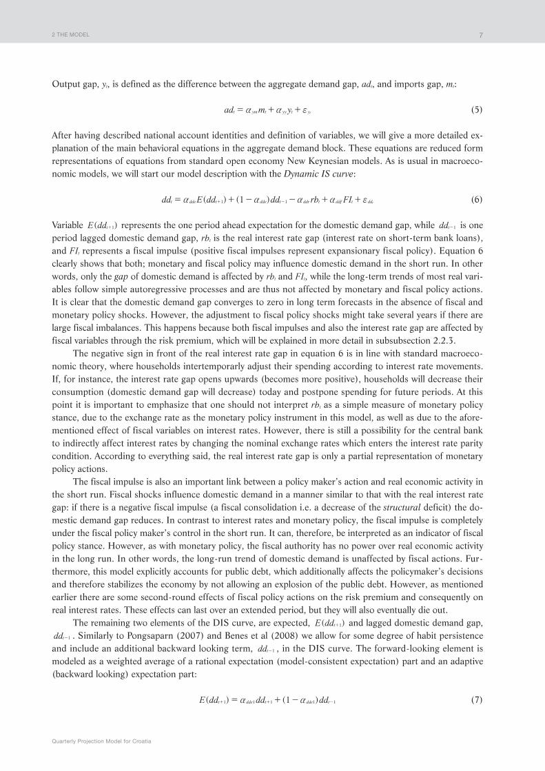
Output gap, yt, is defined as the difference between the aggregate demand gap, adt, and imports gap, mt:
ad m yt ym t yy t yta a f= + + (5)
After having described national account identities and definition of variables, we will give a more detailed ex-planation of the main behavioral equations in the aggregate demand block. These equations are reduced form representations of equations from standard open economy New Keynesian models. As is usual in macroeco-nomic models, we will start our model description with the Dynamic IS curve:
( ) ( )dd E dd dd rb FI1t dde t dde t ddr t ddf t dd1 1 ta a a a f= + - - + ++ - (6)
Variable ( )E ddt 1+ represents the one period ahead expectation for the domestic demand gap, while ddt 1- is one period lagged domestic demand gap, rbt is the real interest rate gap (interest rate on short-term bank loans), and FIt represents a fiscal impulse (positive fiscal impulses represent expansionary fiscal policy). Equation 6 clearly shows that both; monetary and fiscal policy may influence domestic demand in the short run. In other words, only the gap of domestic demand is affected by rbt and FIt, while the long-term trends of most real vari-ables follow simple autoregressive processes and are thus not affected by monetary and fiscal policy actions. It is clear that the domestic demand gap converges to zero in long term forecasts in the absence of fiscal and monetary policy shocks. However, the adjustment to fiscal policy shocks might take several years if there are large fiscal imbalances. This happens because both fiscal impulses and also the interest rate gap are affected by fiscal variables through the risk premium, which will be explained in more detail in subsubsection 2.2.3.
The negative sign in front of the real interest rate gap in equation 6 is in line with standard macroeco-nomic theory, where households intertemporarly adjust their spending according to interest rate movements. If, for instance, the interest rate gap opens upwards (becomes more positive), households will decrease their consumption (domestic demand gap will decrease) today and postpone spending for future periods. At this point it is important to emphasize that one should not interpret rbt as a simple measure of monetary policy stance, due to the exchange rate as the monetary policy instrument in this model, as well as due to the afore-mentioned effect of fiscal variables on interest rates. However, there is still a possibility for the central bank to indirectly affect interest rates by changing the nominal exchange rates which enters the interest rate parity condition. According to everything said, the real interest rate gap is only a partial representation of monetary policy actions.
The fiscal impulse is also an important link between a policy maker’s action and real economic activity in the short run. Fiscal shocks influence domestic demand in a manner similar to that with the real interest rate gap: if there is a negative fiscal impulse (a fiscal consolidation i.e. a decrease of the structural deficit) the do-mestic demand gap reduces. In contrast to interest rates and monetary policy, the fiscal impulse is completely under the fiscal policy maker’s control in the short run. It can, therefore, be interpreted as an indicator of fiscal policy stance. However, as with monetary policy, the fiscal authority has no power over real economic activity in the long run. In other words, the long-run trend of domestic demand is unaffected by fiscal actions. Fur-thermore, this model explicitly accounts for public debt, which additionally affects the policymaker’s decisions and therefore stabilizes the economy by not allowing an explosion of the public debt. However, as mentioned earlier there are some second-round effects of fiscal policy actions on the risk premium and consequently on real interest rates. These effects can last over an extended period, but they will also eventually die out.
The remaining two elements of the DIS curve, are expected, ( )E ddt 1+ and lagged domestic demand gap, ddt 1- . Similarly to Pongsaparn (2007) and Benes et al (2008) we allow for some degree of habit persistence and include an additional backward looking term, ddt 1- , in the DIS curve. The forward-looking element is modeled as a weighted average of a rational expectation (model-consistent expectation) part and an adaptive (backward looking) expectation part:
( ) ( )E dd dd dd1t dde t dde t1 1 1 1 1a a= + -+ + - (7)

2 THE MODEL
Nikola Bokan, Rafael Ravnik
8
Expected values for most other variables are defined in a similar manner.Being more precise about the interpretation of the IS curve, equation 6 represents only the closed-econo-
my part of the IS curve, while we need to define an export function in order to completely define aggregate de-mand and the open economy IS curve. Export gap, or gap of foreign demand for Croatian goods and services depends on foreign (euro area) output gap, ytEA and the real exchange rate gap, zt:
x y zt tEA
xz t xta f= + + (8)
The real exchange rate in this paper is expressed as nominal exchange rate multiplied by foreign to domestic price ratio, expressed in logarithms:
Z S P Pt tEA
t= + - (9)
The import gap is described by the following equation:
( )m y rmcm rmcyt t my t t mta f= - - + (10)
Where rmcmt represents importer’s real marginal cost and rmcyt domestic producer’s real marginal cost. Al-though both marginal costs are simply defined by two identities: rmcm zt t= t and, we use the term marginal costs and the variables rmcmt and rmcyt because they indeed mimic marginal costs in this particular case.12 For example, if real marginal cost for importers is above the real marginal cost for domestic producers, the imports gap will decrease. The opposite is also true: if it is more expensive to produce at home than import products from abroad then the imports gap will increase. Consequently, equations 8 and 10 form import-export rela-tions with the standard reaction to real exchange rate movements: higher real exchange rate gaps are related to higher export gaps and lower import gaps and vice versa, where the net effect will depend on the particular calibration and other mechanisms in the model. The demand effect is also standard: higher domestic demand leads to an increase of imports, while higher foreign demand increases exports. At this point it is once again important to emphasize that this mechanism applies for the short run only, due to the independent movements of the long-run trends of these variables. Using this short- vs. long-run distinction, the model is able to explain an interesting fact about the convergence process during the pre-crisis period; real exchange rate appreciation together with a steep upward trend in exports.
2.2.2 Aggregate supply and price settingInflation in our QPM is represented by annualized changes of the overall consumer price index. As al-
ready mentioned, inflation is modeled by an open economy version of the New Keynesian Phillips curve:13
( ) ( )E oilm rmc1t oil t t oil t rmc t1 1 1 1 tr i i r i r i i fD= - - + + + +r r r r r r+ - (11)
The variable ( )E t 1r + represents one quarter ahead expected inflation, t 1r - one quarter lagged inflation, oilmtD change of imported oil prices and rmct represents the overall real marginal cost. For a complete understanding of the price setting behavior in this model, we have to define rmct.
QOIL OIL Pt t tEA= - (12)
( )rmc rmcy rmcm qoilt rmcy t rmcm rmcqo t rmcqo ti i i i= + - + (13)
12 The variable Z tW presents the real exchange rate gap, with smoothed European prices.
13 Krznar (2011) estimates a New Keynesian Phillips curve for the Croatian economy which is similar to the one used in this paper.

2 THE MODEL
Quarterly Projection Model for Croatia
9
where overall marginal cost is a weighted average of the domestic producer’s real marginal cost, importer’s real marginal cost and real oil prices gap.
The first element on the right-hand side of the Phillips curve represents one-quarter-ahead expectation of CPI inflation. Due to the importance of price stickiness an additional element of lagged inflation is included in the Phillips curve.14 Real activity i.e. output gap enters the Phillips curve via overall real marginal cost. It is almost needless to emphasize that both parameters, rmcyi and rmcir , are positive, due to the positive reaction of inflation to excessive demand. The remaining terms of the Philips curve ( oilmtD , rmcmt and qoilt) are foreign factors that determine domestic prices. We included these terms due to the empirical fact that Croatian prices are largely influenced by foreign ones (Krznar and Kunovac, 2010). Crude oil prices in this model may be in-terpreted as a proxy for all other energy prices, especially gas prices that are highly correlated with oil prices. Moreover, since the oil prices enter the model in euro, changes in the euro to US dollar exchange rate can also affect domestic inflation. The importance of the mentioned US dollar exchange rate for inflation in Croatia and other Central and East European countries is empirically confirmed in Jankov et al (2008).
2.2.3 Monetary policy, exchange rate and financial sectorFinancial sector and interest rates
In contrast to standard monetary models where the UIP condition determines the exchange rate and a re-action function defines interest rate dynamics, for our QPM the opposite is true so that the monetary authority has only limited control over interest rates. Hence, the UIP relation captures the nominal short-term interest rate (short-term Treasury bill rate in this case) dynamics.
( )( ( ( ) ) )NI NI I E S S PREM1t NI t NI tEA
t t t NI1 1 tz z f= + - + - + +- + (14)
The second term on the right-hand side of equation 14 suggests that the domestic short-term interest rate equals the foreign short-term interest rate (3 month Euribor) plus expected nominal depreciation plus some unobserved risk premium ( ( ) )E S S I PREMt t t
EAt1 - + ++ . Additionally, to allow for persistence in interest rate dy-
namics one quarter lagged interest rate, NIt 1- , is included in this equation. This lag is similar to the so-called smoothing term included in most Taylor rules in applied structural models. According to the UIP relation, international investors will equalize expected returns on investments in euro area assets and expected returns on Croatian assets adjusted for expected depreciation and a country specific risk premium. Consequently, an expected depreciation of the kuna will lead to higher domestic interest rates. Equivalently, if the risk premium is positive, investors will demand higher interest rates for Croatian assets, relative to interest rates on European equivalents. It is important to note that the risk premium is an unobserved variable in our model which can, in the same way as other variables, be decomposed to its trend PREMt , and gap, premt. The trend is a simple AR process with a constant steady state level, PREMSS while the risk premium gap is defined by the following equation:
prem DEF DEF DEF DEFDEF prem4t prdef
tS
tS
tS
tS
SSS
prlag t prem1 2 3
1 tz z f= + + +- + +- - -
-b l (15)
where DEFtS stands for structural deficit and DEFSSS its steady-state value or sustainable deficit level. This equation indicates that deficits above their sustainable level are leading to higher risk premium levels, while rel-atively small deficits or surpluses are causing low risk premium levels. We used structural deficit over a period of one year in order to smooth the short-run quarterly deficit dynamics. The equation above shows how fiscal variables can affect the risk premium and consequently interest rates, as mentioned earlier. The equation sug-gest that the risk premium gap will not close as fast as other gaps if we, for example, exogenously impose into our forecasting exercise that structural deficit is above its steady state level during several years of the forecast horizon.
14 A detailed analysis of price stickiness, based on a firm survey, is given in Kunovac and Pufnik (2013).

2 THE MODEL
Nikola Bokan, Rafael Ravnik
10
The trend real UIP relation defines the trend of real short term interest rates,15 RIt as the sum of the for-eign steady state real interest rate, trend of the expected real depreciation and risk premium trend:
( )RI R E Z PREMt SSEA
t t1D= + ++ (16)
As equation 16 clearly suggests, real domestic interest rates are not only in the short-run, but also in the long run determined by foreign interest rates.
The treasury bill rate, NIt, described earlier, is an important building block of our model because it cap-tures the borrowing cost of the government which will at least partially be reflected in the borrowing cost of the entire economy. However, this interest rate cannot be used as the rate that influences domestic demand directly due to the fact that the business and household sectors typically pay higher interest on their debt than the government. In order to take this risk into account, we introduced an additional interest rate that better ex-plains domestic demand movements. For this purpose short-term interest rate on bank loans (client’s rate), NBt is used and it is related to the treasury rate by the following equation:
( ) ( )NB NB NI SPREAD1t NB t NB t t NB1 tz z f= - + + +- (17)
This simple relation states that the bank loan interest rate, NBt is determined by the treasury bill rate plus some unobserved difference, SPREADt. As in some other variables in our model, the bank loan rate has also a backward looking part capturing persistence in interest rate dynamics. The long-run component of spread, SPREADt , is defined as the difference between the trends of the two domestic interest rates, while the short-run component (gap) of the spread is modeled by the following equation
( )spread spread NPL NPL nplt sp t spnpl t SS spnpl t sp1 2 tz z z fD= + - + +- (18)
where the autoregressive process is augmented with the change in non-performing loans (NPLs), npltD and their deviation from steady state, NPLSS.16 The positive parameter related to npltD indicates rising borrowing costs when the share of NPLs increases. This equation captures the effect of private sector default risk on the interest rate spread and consequently on bank lending rates entering the IS curve.
NPLs evolve according to the following equation.
( ) ( )
( ( )( )
( ) ( )
NPL NPL Y Y y y
S S S
RB RB NPL NPL
1
t t NPLY t SS NPLy t t
NPLS NPLSdev t ttar
NPLSdef t
NPLRB t t NPL t SS NPL
1 1 1 2
1
3 4 1 t
z z
z z z
z z f
D D
D
= - - - - +
+ - + - +
+ - + - +
- - - -
-
- - -
r
6 @ (19)
Note that not only short-term ( )y yt t1 2-- - , but also long-term dynamics in output ( )Y Yt SS1D D-- negatively af-fect NPLs. Hence we assume that a slowdown in potential output may have adverse effects on NPLs. Real interest rate changes enter the equation with a positive sign, with an obvious relationship between these two variables postulating higher default risk if interest rates are increasing. As already stated in the introduction, the aim of this paper is to model the main relationships specific to the Croatian economy, one of which is the high degree of credit euroization. One particular mechanism of how the mentioned euroization can affect fi-nancial stability and consequently the entire economy is through the so-called balance sheet effect of exchange rate changes. The idea behind this relationship is that a significant nominal depreciation might cause an in-crease of the existing stock of debt, if a high percentage of loans is denominated in foreign currency (euros in this model). As a consequence of such depreciation, the share of NPLs will increase due to the default of some borrowers that cannot repay their debts. Precisely this mechanism is mimicked by the fourth term on the right-hand-side of equation 19.
15 The trend real Treasury bill rate is defined as: RI NIt t ttarr= - where NIt represents trend of the nominal rate while represents the implicit inflation target
which will be defined later in the paper.
16 The variable nplt is defined as the ratio of non-performing loans to total loans.

2 THE MODEL
Quarterly Projection Model for Croatia
11
The real counterpart of NBt is denoted by RBt and defined as ( )RB NB Et t t 1r= - + . This variable is used to define the real interest rate gap, rbt which affects the aggregate demand gap through the dynamic IS curve as specified earlier (equation 6).
Exchange rate and monetary policyAfter having listed all equations that are necessary for understanding of the interest rate dynamics in our
model, we will move to the explanation of the exchange rate reaction function along with the corresponding in-flation and exchange rate targets:17
( )S SS S S S
1 4ttar
star tSStar
start t t t1 2 3 4z z= + -+ + +- - - - (20)
S StSStar
SStar tSStar
tSStar
1z fD D= +- (21)
S Zttar
ttar
t SSEAr rD D= - + (22)
( ) ( )E Ettar
t ttar
1 1r r r= -+ +% (23)
( ) ( ) ( )S E S S E S1t t S ttar
S ttar
t S1 1 tz r z f- =- + - - ++ +6 @% (24)
The exchange rate target, Sttar , in equation 20 is partly determined by past movements of the exchange rate itself, as well as by some “steady state” variable, StSStar . There are generally two possible definitions of the “steady-state” exchange rate level that are reflecting two different approaches to exchange rate policy. The first, and more restrictive, possibility would be to define a fixed steady-state value which means that the central bank explicitly targets a pre-specified level of the nominal exchange rate. The second, and more flexible, pos-sibility is to define StSStar as a drifting variable which is depicted by equation 21. The choice between these two options is crucial because this variable determines the distance between the actual exchange rate and its target in each period, and therefore it directly affects other variables like the implicit inflation target, interest rates, the real exchange rate gap and indirectly all other variables in the system. We will choose the second approach because the Croatian National Bank (CNB) has never explicitly committed to any fixed exchange rate level. Its policy is rather smoothing exchange rate movements by not allowing strong positive or negative jumps, due to the possible balance sheet effect and due to the pass-through of foreign prices. It is well known that the CNB managed the nominal exchange rate around different levels during the last two decades, and there is no reason to assume that future exchange rate levels will be the same as those 10 years ago. Therefore, exchange rate forecasts produced by our model will not converge to some historical average that might not be relevant for the recent period. Moreover, our flexible modeling approach even offers the possibility of specifying a given future path of the exchange rate level which the central bank aims to target in the future. The steady state exchange rate represents the exchange rate level that the central bank considers to be sustainable in the long run, implic-itly taking into account indicators such as net exports, sustainability of foreign debt, foreign reserves and other relevant variables. Hence, any change in StSStar has to be interpreted as a change in some of these underlying fundamentals. As one can see from the equations above, we are not explicitly defining the target using these fundamentals, but we may impose it implicitly in forecasting exercises.
On the other hand, the inflation target is not explicitly defined and announced, it is rather implicitly determined such that it is consistent with the exchange rate target (equation 22). More precisely, the infla-tion target is defined as the difference between the change of nominal exchange rate target and the change of trend real exchange rate depreciation plus foreign steady state inflation. This means that in the long-run, when SttarD equals zero (note that Sttar is defined in levels), the inflation target equals foreign steady-state inflation
minus trend real depreciation. If there is neither real appreciation, nor depreciation in the long-run (which we can impose through the calibration of steady state values), the domestic inflation target and, consequently,
17 Throughout the paper the exchange rate will represent the HRK/EUR exchange rate.

2 THE MODEL
Nikola Bokan, Rafael Ravnik
12
domestic inflation converges towards the EA inflation target (close but below 2 percent).The last equation of the block (equation 24) above represents the exchange rate reaction function. Ac-
cording to this equation, the monetary authority tries to keep the expected exchange rate close to the smoothly moving target, but it will also react to inflation deviations from its implicit target. Both of these deviations are forward-looking variables. Thanks to such a specification the monetary authority in our model makes deci-sions about the policy instrument (nominal exchange rate) today by considering what is likely to happen in the future. This resembles the idea about the central bank stabilizing (anchoring) exchange rate expectations and consequently inflation expectations.
To provide an understanding of the monetary policy mechanism, let us first consider an illustrative exam-ple where 0Sz = as an extreme case. It is easy to see that in the absence of shocks to this equation, the nomi-nal exchange rate would always equal its targeted level which means that the central bank perfectly controls exchange rate expectations which represents a fixed exchange rate regime. Nonetheless, in practice we will use a parameter value such that 0 1< <Sz . For realistic calibrations in this range, the central bank manages the exchange rate by keeping it as close as possible to the targeted level, but allowing for some degree of variation, while at the same time taking into account inflation movements. Consider the example where expected infla-tion rises above its target: the central bank in this model will react by appreciating today’s nominal exchange rate, due to the negative sign in front of t
tarr% . This appreciation will dampen the inflation pressure and move
it towards its target level through two different channels. First, note that the exchange rate enters the open economy Phillips curve (equation 11) with a positive sign, which implies that the mentioned appreciation will put additional pressure on a decrease in inflation. Due to the assumed price stickiness, the process of return-ing expected inflation to target will take several quarters. Moreover, there is also an interest rate channel that is influenced by the mentioned exchange rate changes. As the inverse of the left-hand side of equation 24 enters the UIP relation (equation 14), nominal T-bill interest rates will increase, leading to an increase in nominal lending rates. The net effect on real lending rates is not a priori clear and it will depend on the calibration and other model mechanisms.
In order to give a further explanation of equation 24, consider the case where the economy is in steady state and a positive exchange rate shock Stf hits the system. This would increase (depreciate) the exchange rate today, but according to the mentioned equation an appreciation will follow immediately in the next period so that the exchange rate level stays close to its target. This mechanism ensures that the nominal exchange rate never drifts far away from the targeted level. The impulse response functions for this shock are shown in the appendix and will be explained in more detail in section 5.
2.2.4 Fiscal sectorThe fiscal sector is the remaining building-block of this QPM. It is included in the latest version of our
model due to the increasing importance of fiscal policy actions during the period of fiscal stress and the associ-ated excessive deficit procedure (EDP).
The fiscal sector used here is a simplified version of the one described in OG research (2011). Our model captures both directions of real-fiscal interactions. The first direction is related to the question about how real economic activity affects fiscal variables. For this purpose we are explicitly modeling the cyclical component of the overall government deficit. Modeling the reverse direction means finding a way from discretionary fis-cal policy actions to economic activity. This is done by equation 6, which describes how fiscal impulses affect domestic demand. Fiscal variables can additionally affect real variables through the risk premium and interest rates which are captured by equation 15.
In this paragraph fiscal variables are defined, while the structural equations are explained below. It is im-portant to note that the two observed fiscal variables, general government debt and deficit, are expressed as shares in annual nominal GDP. Additionally, instead of the budget balance, we are using fiscal deficit, which means that we interpret positive numbers as deficits, and negative numbers as surpluses. The first equation shown below is a standard definition of cyclical deficit, DEFtC :
DEF y ddtC
Cy tan
Cdd tand d= + (25)
2 THE MODEL
Quarterly Projection Model for Croatia
13
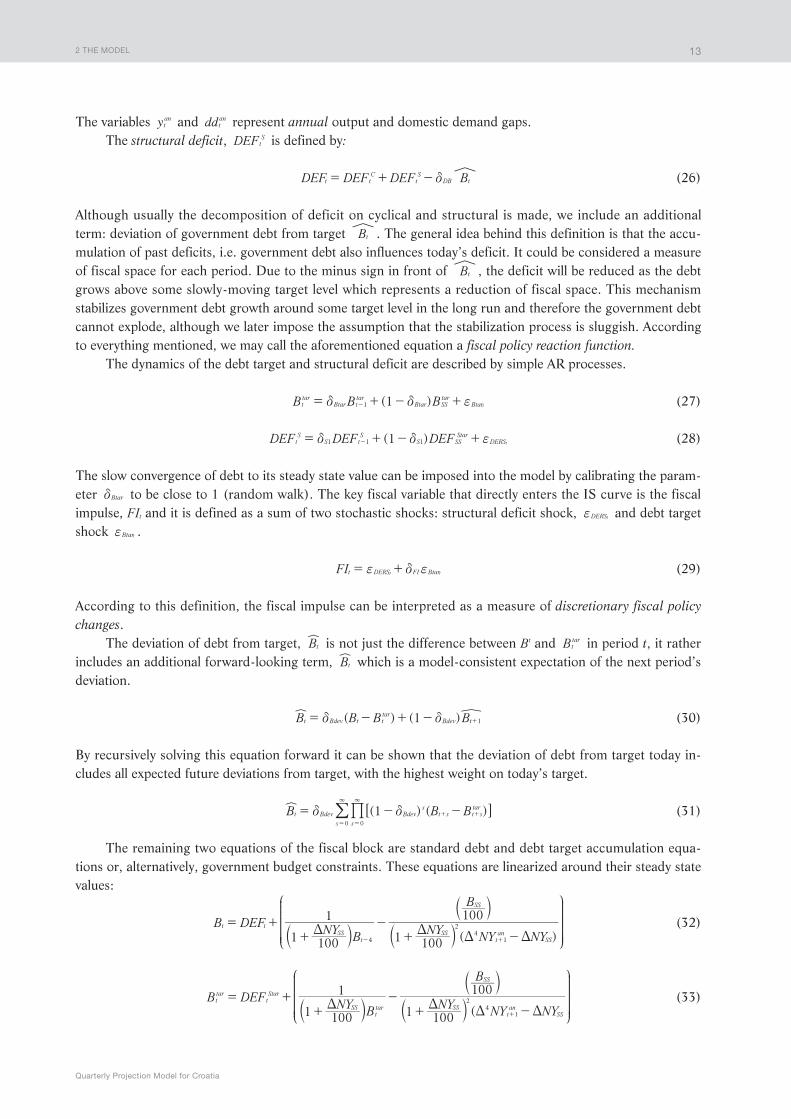
The variables ytan and ddtan represent annual output and domestic demand gaps.The structural deficit, DEFtS is defined by:
DEF DEF DEF Bt tC
tS
DB td= + - % (26)
Although usually the decomposition of deficit on cyclical and structural is made, we include an additional term: deviation of government debt from target Bt% . The general idea behind this definition is that the accu-mulation of past deficits, i.e. government debt also influences today’s deficit. It could be considered a measure of fiscal space for each period. Due to the minus sign in front of Bt% , the deficit will be reduced as the debt grows above some slowly-moving target level which represents a reduction of fiscal space. This mechanism stabilizes government debt growth around some target level in the long run and therefore the government debt cannot explode, although we later impose the assumption that the stabilization process is sluggish. According to everything mentioned, we may call the aforementioned equation a fiscal policy reaction function.
The dynamics of the debt target and structural deficit are described by simple AR processes.
( )B B B1ttar
Btar ttar
Btar SStar
Btar1 td d f= + - +- (27)
( )DEF DEF DEF1tS
S tS
S SSStar
DERS1 1 1 td d f= + - +- (28)
The slow convergence of debt to its steady state value can be imposed into the model by calibrating the param-eter Btard to be close to 1 (random walk). The key fiscal variable that directly enters the IS curve is the fiscal impulse, FIt and it is defined as a sum of two stochastic shocks: structural deficit shock, DERStf and debt target shock Btartf .
FIt DERS FI Btart tf d f= + (29)
According to this definition, the fiscal impulse can be interpreted as a measure of discretionary fiscal policy changes.
The deviation of debt from target, BtX is not just the difference between Bt and Bttar in period t, it rather includes an additional forward-looking term, BtX which is a model-consistent expectation of the next period’s deviation.
( ) ( )B B B B1t Bdev t ttar
Bdev t 1d d= - + - +X \ (30)
By recursively solving this equation forward it can be shown that the deviation of debt from target today in-cludes all expected future deviations from target, with the highest weight on today’s target.
( ) ( )B B B1t Bdev Bdevs
t s t star
ss 00
d d= - -33
+ +
==
6 @X %/ (31)
The remaining two equations of the fiscal block are standard debt and debt target accumulation equa-tions or, alternatively, government budget constraints. These equations are linearized around their steady state values:
( )
B DEFNY
BNY
NY NY
B
1 100
1
1 100
100t t
SSt
SStan
SS
SS
4
24
1D D
D D= +
+-
+ -- +
J
L
KKKKKKKKb bb N
P
OOOOOOOOl ll
(32)
(
B DEFNY
BNY
NY NY
B
1 100
1
1 100
100ttar
tStar
SSttar SS
tan
SS
SS
24
1D D
D D= +
+-
+ -+
J
L
KKKKKKKKb bb N
P
OOOOOOOOl ll
(33)

3 CALIBRATION
Nikola Bokan, Rafael Ravnik
14
3 Calibration
In this section we explain our choice of parameter values for the baseline calibration. The parameters in our model can be divided into two groups: i) exogenous steady-state values which determine trend vari-ables and ii) parameters in behavioral equations related to the gaps influencing business cycle properties of the model. The baseline calibration for all parameters is given in the appendix, while below those most relevant are explained in more detail.
3.1 Calibration of steady-state values
As already said in the previous section, the growth rates of all variables in the model converge in the long-run to their respective steady-state values. Most of these steady-state growth rates are calibrated explic-itly, while some of them are defined through basic identities. When calibrating these values we tried to capture some historical characteristics of each series (for example average growth rates), while at the same time being theoretically consistent. At this point it is important to note that Croatia is a post-transition country that went through significant changes in its economy and institutions, which is also reflected in trends of some of the analyzed variables. These changes introduce additional difficulties into the process of calibrating steady-state values. The calibration exercise is hence a balance between fitting past observations as well as possible but at the same time putting more emphasis on the recent period in order to perform well in forecasting exercises.
The steady-state value of real output growth is calibrated at 2.5%. The observed average growth rate of GDP is somewhat below this value, but this average is strongly influenced by a prolonged period of negative growth rates between 2008 and 2014. Since at least a part of this decline can be considered cyclical we choose this higher value given the recent above-average GDP growth.
It is assumed that import steady-state growth equals export steady-state growth which means that we do not allow trade deficits or surpluses in the long run. A growth rate of 4.5% is chosen for these two variables. It is easy to see that there is some inconsistency between the calibrated steady state growth rates of GDP on one side and exports and imports on the other side. Using such a calibration the ratio of imports and exports to GDP will grow without bounds in the very long-run. However, for our forecasting applications this is not an important issue since we are focusing on a forecast horizon of around 5 years and for this period we are still not expecting a slowdown in the trend growth rates of exports and imports with respect to the trend growth rate of GDP.
Due to the open economy nature of our model, some of the assumptions about foreign variables are di-rectly transmitted into domestic ones. For example, the trends of domestic interest rates are directly influenced by foreign interest rates. As we explained in the model description, the nominal T-bill interest rate equals the European nominal risk-free interest rate plus expected depreciation plus a risk premium. In a steady state without nominal depreciation the T-bill interest rate will, thus, equal the European steady state interest rate plus the steady state risk premium. We set the European real interest rate at 0.5 (EA inflation steady state is 1.85) and hence the nominal one at 2.35 which is close to the historically observed average. The steady state risk premium is set at 0.75. Consequently, the steady state value for the nominal T-bill interest rate is 3.1. The spread steady state level is 4.5, which means that the bank lending rate equals 7.6 in steady state. These values are, like the previous ones, chosen according to the respective historical averages.
We assume zero real depreciation in the long run, even though negative growth rates (average real ap-preciation) for the real exchange rate is observed during a prolonged period between 2002 and 2010, due to continuously higher inflation rates in Croatia in comparison to the euro area. This phenomenon of an ex-tended period of real appreciation is also present in other post-transitional countries especially in Central and Eastern Europe (Benes et al, 2008). Various possible explanations for such behavior can be found, including the well-known Balassa-Samuelson effect. However, it has been shown that this effect is not significant for Croatia (Funda et al, 2006) and moreover during the crisis period the real exchange rate depreciated due to a

3 CALIBRATION
Quarterly Projection Model for Croatia
15
combination of low domestic inflation and mild nominal depreciation. We will accordingly assume zero growth of the real exchange rate in the long run.
Steady state inflation is also determined through foreign steady state inflation which is set at 1.85% which is in line with the observed average inflation and at the same time this value reflects the ECB’s target of being below, but close to, 2%. Through the trend real UIP relation, the inflation target equals foreign steady-state inflation target minus trend real depreciation. As already mentioned in the previous section, due to zero real depreciation in the long run, the domestic inflation target, therefore, converges to the foreign inflation target. Consequently, domestic inflation will converge to 1.85% in the long run.
The steady state level of non-performing-loans is calibrated at 10% which approximately equals the ob-served sample average.
The calibration of steady state levels for fiscal values is influenced by our view about the long-term goals of the fiscal policy maker and the current institutional setting. For example, the Maastricht criteria are impor-tant factors. However, there is a tradeoff between matching this criteria and producing precise medium term forecasts. Due to the public debt accumulation dynamics observed during the last decade it is not realistic to assume that the debt level will return to levels close to 60% of GDP, at least not during a typical forecast hori-zon. Therefore we calibrated the steady state level of public debt at 70%. In order to converge to this level, we calibrated the steady state public deficit using the definition of deficit level that is sustainable in the long run, which amounts to 2.9% using the most recent data.
3.2 Calibration of business-cycle parameters
As in Berg et al (2006) the calibration of parameters that determine the short-run movements is based on three main criteria: i) economic theory, ii) stylized facts about the analyzed economy and iii) international experiences obtained from the related literature. The calibration of this set of parameters is an iterative proce-dure that takes all three criteria into account while at the same time keeping track of the meaningfulness of the estimated filtered series and the impulse response functions.
The Phillips curve, IS equation and policy rule represent the core of our model and the parameters of these equations are therefore crucial for the behavior of the forecasts produced by this model. Our aim was to find robust values for these parameters such that new versions of the model do not require significant changes to the calibration shown in the present paper.
For the dynamic IS curve we introduced some degree of habit persistence in order to produce relatively smooth values for domestic demand as observed in the data. We therefore put 0.7 weight on the backward looking part and 0.3 at the forward looking part. The values for the remaining two parameters ddra and ddfa are 0.13 and 0.5, respectively. The relatively low value for the parameter ddra is a consequence of the empirical fact about the Croatian economy where real activity reacts rather mildly to interest rate changes.
For import and export gaps the demand effects dominate over price effects as shown in Bobić (2010). Due to this empirical evidence, the parameter in front of domestic and foreign output gap equals one, while the values for parameters xza and mya related to the real exchange rate gap are set bellow one (0.65 and 0.75 respectively).
The open economy Phillips curve is calibrated to match Croatian inflation data. We set oilir to 0.015, 1ir to 0.1 and rmcir to 0.25. This calibration reflects low inflation persistence in comparison with the standard val-ues chosen in the literature. This is not surprising due to the monetary policy regime, where the exchange rate is targeted and therefore, according to monetary theory, the inflation rate has a rather high variance in com-parison to inflation targeting regimes. A value of 0.25 for rmcir in combination with only 0.72 for rmcyi reflects a relatively flat Phillips curve for Croatia. The elasticity of inflation to oil price changes is captured by param-eters oilir and .0 1rmcqoi = which are estimated using a satellite regression.
We calibrated the parameters of the exchange rate reaction function in such a way that a larger weight is put on the exchange rate deviation and a smaller weight on the inflation deviation, and therefore parameter Sz equals 0.2. As already shown in the previous section, the exchange rate target is a weighted combination
4 FORECASTING
Nikola Bokan, Rafael Ravnik
16
of past exchange rate levels and a slow-moving steady state level. In order to keep this target smooth enough we put more weight on its steady state level ( . )0 6starz = . The growth rate of this steady state level follows a stationary autoregressive process with an AR coefficient, SStarz of 0.2. The aim of this low AR coefficient is to force the nominal exchange rate forecast to stabilize close to the observed end-of-sample level for the respec-tive sample. Results obtained from forecasting exercises are supportive of this parameterization. It is, however, possible to impose specific assumptions about future dynamics of the exchange rate level or its target and therefore force the exchange rate to converge towards any desired level.
For the UIP and for equation 17 we calibrated parameters NIz and NBz at 0.5 and 0.35 respectively. This choice of parameters reflects the empirical fact that the T-bill is less persistent in than the bank lending interest rate. For the spread equation the following parameterization is used: .0 6spz = , .0 075spnplz = , .0 075spnpl2z = so that the same weight is put on the deviation of NPLs from steady state and the growth rate of NPLs. The same value for the AR coefficient for the risk premium is chosen and by using historical data on the government deficit we estimated the coefficient prdefz to be 0.05. The equation for NPLs is also estimated and the following parameter values are obtained: .0 15NPLYz =r , .0 25NPLyz = , .0 7NPLSz = , .0 2NPLRBz = , .0 04NPLz = , .0 8NPLSdevz = . Hence, the exchange rate becomes an important driving force for the NPL dynamics in this economy.
As shown in equation 29 the fiscal impulse is not only a shock to the structural deficit equation; it is also extended by a deficit target shock. The weight on this second shock (parameter FId ) is approximately 10% of the weight on the structural deficit shock. This parameterization is in line with OG Research (2011) where a similar fiscal impulse definition is used. For the debt deviation equation also, the parameterization is borrowed from OG Research (2011), with .0 3Bdevd = . The automatic stabilizer effect (parameter DBd ) in equation 26 is set at 0.05. This relatively small parameter value reflects the observed behavior of past governments where limited weight is put on the debt level when making decisions about the current budget. The elasticities of the government deficit with respect to output gap and domestic demand gap ( .0 49Cyd =- and .0 43Cddd =- ) are estimated using the standard methodology with data on individual components of budget revenue and expend-iture. In order to impose slow convergence of debt to its steady state value we calibrated the parameter Btard to be very close to a random walk process, i.e. 0.995.
4 Forecasting
All model equations described above are written in state-space representation after which the Kalman filter is used to estimate the unobserved variables and shocks taking into account observed data. The block of domestic observables includes real and nominal GDP, real exports and imports of goods and services, CPI in-flation, kuna to euro exchange rate, T-bill interest rate (up to 1 year maturity), bank lending interest rate (up to 1 year maturity), ratio of non-performing to total loans, general government overall deficit and debt, while the block of foreign variables includes European real GDP and output gap, 3 month Euribor, European HICP inflation, USD to euro exchange rate and Brent crude oil prices.
The resulting estimates of unobserved variables and shocks are used as initial conditions for the forecast-ing exercise. As already emphasized, the main application of the model is to produce medium-term forecasts within a consistent framework. We usually assume a 5-year forecasting horizon when referring to the medium-term. In this section two standard forecasting approaches are explained. The first one puts more weight on the information produced by the model itself and we will refer to it as Baseline forecast. This forecasting approach uses only a very limited set of judgmental inputs. The second, and from a practical point of view, more con-venient approach conditions on assumptions about a given path of some variables and it is called Conditional forecast. Both forecasting approaches are used in practice when running the model for forecasting exercises.

4 FORECASTING
Quarterly Projection Model for Croatia
17
4.1 Baseline forecast
Although the first forecasting approach is called Baseline it is by no means a pure model-based forecast. We will rather condition the model forecast on exogenous paths for a narrow set of variables. Conditioning variables are usually those that cannot be suitable forecasted by the model. The main reason for using exog-enous forecasts for these variables is the small-open-economy setup of the present model. More precisely, in order to forecast domestic variables using this QPM, one needs forecasts of foreign variables. For this purpose forecasts from external sources are usually used, such as forecasts from other institutions, which are combined in a separate QPM for the EA economy. Due to this reason, our Baseline forecast will in practical applications condition on an exogenously given path of European output gap, inflation and interest rate as well as crude oil prices and USD/EUR exchange rate. All mentioned exogenous forecasts are included in the model for the entire forecasting horizon. Moreover, we usually augment the dataset with a nowcast of domestic GDP. Using such a nowcast can be useful due to the availability of high frequency data for the first quarter of the forecast-ing horizon and the superior performance of high-frequency nowcasting models in the very short run as de-scribed in Kunovac and Špalat (2014). Conditional on the mentioned exogenous forecasts and the estimated initial conditions, the model will produce forecasts for all other variables for the respective forecasting horizon.
4.2 Conditional forecast
The Conditional forecast takes a broader set of exogenous information into account when producing forecasts. In addition to the above mentioned set of foreign variables one can use additional exogenous fore-casts for domestic variables obtained from satellite econometric models, other institutions or expert judgment forecasts. For this purpose not all exogenous information has to be treated completely as given (hard condi-tioning); we can additionally observe some of the exogenous forecasts with a measurement error (soft condi-tioning). The flexible modeling approach allows us to simultaneously use any combination of hard and soft conditioning for any desirable horizon. One example is to assume a given path for the nominal exchange rate (or nominal exchange rate target) for the entire forecasting horizon and produce forecasts for other variables consistent with such a path. This exogenous path of the exchange rate can be either perfectly observed or part-ly observed and it can be combined with assumed future paths for other variables.
In practice it is common to impose soft conditioning on domestic variables only for a short horizon, while letting the model predict the medium run. Such conditional forecasts are used if expert judgment forecasts or satellite model forecasts for some variables are available for the short run. By calibrating variances of the meas-urement errors of these conditioning variables we can impose our belief about the credibility of the mentioned exogenous forecasts. The common set of exogenously forecasted variables used when this model is applied to the Croatian National Bank forecasting exercises are: real GDP up to one year, nominal exchange rate (or its target) for a period of 1 to 3 years, governments deficit up to 2 or 3 years, inflation rate up to one year and if necessary real exports and imports up to one year. These exogenous forecasts are usually produced by experts. It is very likely that the mentioned expert forecasts can outperform any structural model in the very short run, and therefore they can serve as a good starting point for the model over the medium term. On the other hand, for medium term forecasting the underlying structural driving forces of the economy are becoming more im-portant and hence the QPM has significant advantages over simple models or expert forecasts.
In addition to the mentioned conditional forecasts, one can also impose so-called add-factors for some particular observations of interest. These add-factors are residuals that can be added to a variable of interest for some particular period in the future. Suppose, for example that the government announces an increase in the VAT rate (which is not explicitly included in the model) in the first quarter of the forecasting horizon and that we have access to an estimation of the direct contribution of this change to the CPI inflation rate. In this case we could simply use this approximation in order to tune the Phillips curve and run the forecast. Such add-factors are not used in every forecasting round; they will only be used if information about future policy changes is available.

5 MODEL PROPERTIES
Nikola Bokan, Rafael Ravnik
18
4.3 Using the QPM for forecasting exercises in the Croatian National Bank
For the use of our QPM in practical applications for forecasting exercises in the Croatian National Bank, we suggest the use of both Baseline and Conditional forecasts. Each of the mentioned forecasts has it use-fulness depending on the stage of the forecasting exercise. In a very early stage of the exercise, the Baseline forecast, as described above, is run. In the next step, the resulting forecasts are used as an input into various satellite models and expert judgment forecasts. The obtained baseline forecast serves as a broad idea about the direction of some of the main macroeconomic variables in the short- and medium-term future. Any available information which the model is not able to capture can be added to this baseline forecast using the mentioned satellite and judgmental forecasts. In later stages of the forecasting exercise one can use this augmented infor-mation set in order to run the Conditional forecast as explained in the previous subsection. This first version of the Conditional forecast is used to detect inconsistencies between individual forecasts of variables produced by separate satellite models or experts. After discussing such inconsistencies, adjustments are made and the Con-ditional forecast is rerun. This iterative procedure may be repeated several rounds until agreement between all forecasting methods is reached.
5 Model properties
5.1 Impulse response functions
In this section impulse response functions for the most important endogenous variables are shown. The impulse response functions are given in the appendix in figures 4 to 10, where the periods represent quarters. All variables are at their respective steady state levels before the analyzed shocks hit the economy. We will fo-cus only on the following set of exogenous shocks that are interesting for the Croatian economy: exchange rate shock, shock to the exchange rate target, risk premium shock, structural deficit shock, foreign interest rate shock, foreign inflation shock and foreign output gap shock. By analyzing responses to these shocks one can gain a deeper insight into the main relationships and channels that are specific to the Croatian economy and hence to this model. However, as already mentioned, the shocks are not completely structural which has to be kept in mind when interpreting the impulse response functions.
5.1.1 Exchange rate shock and shock to the exchange rate steady stateAlthough equation 24 presents the monetary reaction function, the shock to this equation, stf is not
a monetary policy shock. It can rather be considered a non-fundamental shock to the exchange rate level. However, the shock to the exchange rate steady state level, t
SStarf in equation 21 is closer to a monetary policy shock. The main difference regarding the impact on the exchange rate level is that the former has only a tem-porary effect, while the later has a permanent effect. Namely, a shock to the target means that the central bank decides to target a new exchange rate level, while the shock to the exchange rate equation will immediately be counteracted through the reaction function. As already said earlier the slowly moving steady state exchange rate represents the exchange rate level that the central bank considers to be sustainable in the long run, implic-itly taking into account variables such as net exports, foreign debt, foreign reserves and other relevant indica-tors. Therefore a shock to the target represents a change in the policy maker’s view about the aforementioned level which may be interpreted as a policy shock.
Exchange rate shockThe resulting impulse response functions for the one percentage non-policy exchange rate shock in equa-
tion 24 is shown in figure 4 in the appendix. One can see that the nominal exchange rate depreciation on im-pact is followed by an immediate appreciation in the next quarter due to the reaction function of the central

5 MODEL PROPERTIES
Quarterly Projection Model for Croatia
19
bank. This appreciation in the first period after the shock is relatively strong, although not as strong as the initial depreciation. It will therefore take 5 – 6 more quarters to completely offset this initial depreciation. The response of the one-quarter-ahead exchange rate expectations goes in the same direction as the exchange rate itself, but with a significantly smaller variance. The exchange rate expectation response follows such a smooth pattern due to almost fully rational agents that trust the credible monetary policy of exchange rate smoothen-ing. The exchange rate target response indeed follows a shape and magnitude similar to that of the expected exchange rate response.
This pattern is also transmitted to the implicit inflation target which peaks in the first quarter and reaches its trough four quarters after that. The CPI inflation reacts on impact by 0.18 percentage points, which cor-respondents to an impact pass-through of around 15%. The inflation response decreases thereafter and turns negative one year after the shock. This deflationary pressure is a direct consequence of the nominal FX appre-ciation which stabilizes the price level at its trend. At this point it is worth stressing that the policy of exchange rate level targeting has consequences to the price level similar to those of the policy of price level targeting. The price level (consumer price index) is therefore a trend stationary variable (the CPI slope is the implicit inflation target) where the price level always returns to its trend after temporary deviations.18 For strict inflation target-ing regimes, on the other hand, inflation would return to its targeted inflation rate, which would lead to a per-manent level shift in the CPI.
The combined effect of the inflation and exchange rate reactions becomes evident in the real exchange rate response depicted in the sixth panel of figure 4. As expected, the real exchange rate reaction is dominated by the nominal exchange rate reaction which is stronger than the inflation reaction, leading to a real deprecia-tion. This depreciation of the real exchange rate gap affects the export gap positively and the import gap nega-tively, leading to positive net exports.
Nominal interest rates are also affected by changes in the actual and expected exchange rate level. More precisely, through the UIP condition, the expected appreciation caused by the monetary policy reaction ex-plained above leads to a lower domestic nominal T-bill rate. On the other hand, the initial increase in the nomi-nal exchange rate will cause an increase in the stock of non-performing-loans due to the balance-sheet-effect, which leads to a higher spread. This will put pressure in the opposite direction on the bank lending rates. The net effect in the short run is a modest decrease in the client interest rate (in real terms) followed by a pro-longed period of slightly positive interest rate deviations.
The effect on real activity is shown in the upper right panel in figure 4. Notice that the response of the domestic demand gap is only marginally positive during the first year, after which it turns negative. The re-sponse remains negative during the entire horizon (10 years) with only sluggish convergence towards steady state. It will eventually reach the steady state after approximately 13 years (not shown). This slow convergence is a consequence of at least two channels. The first one is related to the mentioned increase in spread which increases nominal and real interest rates and therefore puts downward pressure on domestic demand through the IS curve. Moreover, the increase in public debt (lower right panel in figure 4) will eventually cause a fiscal consolidation in the medium term in order to return public debt to its targeted level. The mentioned consoli-dation is depicted by the negative structural deficits during the period from the third to the last year. Combin-ing net exports response with the mentioned domestic demand response gives the reaction of the output gap depicted by the blue line in the upper right panel. The positive net export response causes a stronger positive response of the output gap compared to the response of the domestic demand gap during the first few quar-ters. After five quarters the response of the output gap becomes negative as well, although not as negative as the domestic demand gap.
Shock to the exchange rate steady stateAs already argued above the shock to the exchange rate steady state, t
SStarf may be interpreted as a mone-tary policy shock in this model. The resulting impulse response functions to a positive (expansionary) monetary
18 This is in line with the macroeconomic theory, as for example in Gali (2008), where the optimal policy under a pegged (or managed) exchange rate re-gime causes trend stationary in the price level, or stationary for zero inflation steady state models.

5 MODEL PROPERTIES
Nikola Bokan, Rafael Ravnik
20
policy shock are shown in figure 5 in the appendix. Below we emphasize the most striking differences between these responses and those to the non-policy exchange rate shock explained earlier.
First, the monetary policy shock has a long term impact on the level of the exchange rate target and consequently the level of the actual and expected exchange rate. Therefore, no significant deviations from the exchange rate target are observed. After the initial impact of around 0.7 p.p., all three mentioned variables converge to the new steady state level which is around 1.25 p.p. above the initial one. On the other hand, the exchange rate shock explained earlier has only short run effects on the exchange rate level due to the immedi-ate reaction of the monetary policy maker.
Second, the impact on the inflation rate and inflation target is stronger than above. The inflation rate increases on impact by as much as 0.7 p.p. in comparison to 0.18 above. Furthermore, the response of the in-flation target is stronger than before by a factor of approximately 5. These stronger impact responses can be explained by the forward-looking nature of the Phillips curve where most agents are aware of the fact that this change in the nominal exchange rate target is permanent. Due to the fact that this target is directly transmitted into the inflation target the agents expect higher inflation for the next few quarters which will not be offset by a lower-than-steady-state inflation target thereafter. Such a pattern of the inflation target causes a permanent level shift in the price level. This behavior differs to the behavior caused by a non-policy exchange rate shock, where every positive response of the inflation target has to be counteracted by an equivalent negative response of the inflation target in order to return the price level to its trend.
Third, nominal interest rates increase in the short and medium run, while for the non-policy shock above decreases were observed. This increase is a consequence of the expected depreciation, which positively affects both the T-bill rate and the interest rate spread. The former channel works through the UIP relation, and the later through the balance sheet effect due to more NPLs. Notice that the later channel works in the same di-rection as the non-policy shock, while the former works in the opposite direction. This difference in the first channel can, once more, be explained by the rational behavior of the agents in this economy. More precisely, the agents understand the credible monetary policy making process to a large extent and they are, thus, aware of the persistence of the change in the exchange rate after such a policy shock. They consequently expect de-preciations during the first few quarters after the shock. Precisely these depreciations are visible in the interest rate increase mentioned earlier. Although nominal interest rates increase, the real lending rate gap decreases, due to the strong jump in the inflation rate during the first quarters after the shock. Note that this initial drop in the real lending rate is much stronger than earlier, albeit with a similar shape.
Fourth, the real exchange rate remains, like the nominal one, depreciated during an extended period, even though the initial jump is less pronounced than for the non-policy exchange rate shock.
All mentioned differences are carried over to differences in responses of real activity variables. The positive responses of output gap and domestic demand gap (real interest rate decrease) are stronger and long-lasting. These responses peak at about 0.22 p.p. three quarters after the shock and turning slightly negative more than three years after the shock. Imports increase in the short run due to the domination of the demand effect over the price (real exchange rate) effect. On the other hand, exports react in a similar manner as to the previous shock.
5.1.2 Risk premium shockA shock to the risk premium, although not a completely structural one, is of particular interest for the
Croatian economy. It gained particular attention during the European sovereign debt crisis and the period of increased fiscal stress in Croatia. It can be interpreted as an exogenous shift in the risk premium caused for example by spillovers from other countries, as observed during the European sovereign debt crises. As shown in Kunovac (2013) and Kunovac and Ravnik (2017), foreign factors explained more than 50% of Croatian sovereign spreads during the European sovereign debt crisis. These factors are, by construction, unaffected by any domestic economic variables and are, thus, completely exogenous in our model. We can, therefore con-sider these strong spillover factors during the mentioned period as a series of risk premium shocks. In this subsection we analyze the consequences of such a risk premium shock in the context of our QPM. According to everything shown below, we can conclude that the mentioned public debt crises indeed significantly affected the domestic economy.

5 MODEL PROPERTIES
Quarterly Projection Model for Croatia
21
The impulse response functions to a 1 p.p. risk premium shock, premtf are shown in figure 6. This 1 p.p. shock will, under the baseline calibration, through the UIP, lead to an impact increase of the T-bill rate by about 0.5 p.p. This positive effect will die out after approximately 10 quarters. As a consequence of the T-bill rate jump, the real lending rate will also rise by around 0.4 p.p. and peak at the third quarter after which it smoothly returns.
The mentioned increase in the lending rates causes a drop in domestic demand during the first 4 years. This slowdown in domestic economic activity transmits through the Phillips curve into lower domestic infla-tion. As a reaction to such a low inflation rate, the domestic currency depreciates slightly. The real exchange rate depreciates due to this nominal depreciation in combination with low inflation. This raise in competitive-ness causes a positive net-export reaction, which leads to a dampening of the negative impact of domestic de-mand on the output gap.
Lower output in combination with higher borrowing costs will eventually lead to higher deficits during the next five years. Consequently, public debt increases for the entire simulation horizon and beyond, with only sluggish convergence towards its target.
5.1.3 Structural deficit shock – fiscal shockThe fiscal policy maker can affect domestic economic activity through the fiscal impulse which is a
weighted average of a structural deficit shock and public debt target shock (equation 29). In this part of the paper, we will present impulse response functions to the second shock – the structural deficit shock Btartf . We are analyzing a positive shock which represents an expansionary fiscal policy shock.
The lower panel of figure 7 shows the response of fiscal variables to this fiscal shock. Due to the sluggish adjustment of fiscal variables to excessive deficits, this fiscal shock increases the overall and the structural defi-cit during the entire simulation horizon. This increase is also visible in the public debt response, which peaks at 2.3 p.p. during the seventh year. Both responses can be considered as a worsening of the fiscal fundamentals. Such a worsening causes an increase in the risk premium, which in turn raises both interest rates.
The mentioned raise in interest rates partly offsets the positive impact of an expansionary fiscal policy on domestic demand. The net effect is a 0.4 p.p. impact increase in the domestic demand gap, which remains positive for the first 10 quarters. After that, the negative effect of higher interest rates dominates over the posi-tive effect of higher deficits, and consequently the domestic demand gap response becomes negative. Without any significant change in prices or in nominal exchange rates, this pattern is almost completely transmitted into the imports gap response. Consequently, output gap rises on impact less than the domestic demand gap, and equivalently drops more weakly afterward.
5.1.4 Foreign shocksIt is important to emphasis that in this model only the domestic economy and channels between the for-
eign (EA) economy and the domestic one are modeled. However, the foreign economy itself is not explicitly modeled, which means that there is no interaction between variables in the foreign block. All these variables follow simple autoregressive processes. Consequently, a shock to the European interest rate will not dampen European economic activity or inflation, neither will a shock to foreign prices affect any of the other European variables. Hence foreign shocks are by no means true structural shocks, which has to be kept in mind when in-terpreting the impulse response functions.
Foreign interest rate shockAs explained above, the ECB monetary policy is not explicitly modeled in this model, and consequently
we do not consider a shock to the foreign interest rate a monetary policy shock. It is, rather, a non-fundamen-tal shock that raises foreign interest rates and transmits to the domestic economy through the UIP condition, without changing other European variables. The impulse response functions of this shock are shown in figure 8 in the appendix. One can see that the Treasury bill rate rises by approximately 0.6 p.p., which is quantita-tively similar to the risk premium shock. Moreover, almost all other responses are equivalent to the responses to the risk premium shock. We can therefore conclude that an exogenous increase of the risk premium affects

5 MODEL PROPERTIES
Nikola Bokan, Rafael Ravnik
22
the Croatian economy by the same degree as an equal increase in the Euribor rate.
Foreign inflation shockThe empirical literature confirmed that Croatian consumer prices are to a large extent determined
through foreign ones (Krznar, 2011 and Krznar, Kunovac, 2010). It is therefore interesting to demonstrate the effect of changes in foreign prices on domestic prices in the context of the present QPM.
Figure 9 in the appendix show the responses to a 1 p.p. shock to EA inflation. This shock directly affects the marginal cost of importers and thus increases import good prices which, through the open economy Phil-lips curve, increase domestic inflation by approximately 0.5 p.p. in the first quarter. The inflation rate response remains positive for the next 4 years after this initial jump. The central bank reacts to this positive deviation of inflation from its implicit target by appreciating the nominal exchange rate by approximately 0.2 p.p. and keep-ing it below target during the entire 4-year period. Precisely this appreciation, induced by the central bank, causes the inflation rate to return to its targeted level.
The initial appreciation causes a decline in NPLs and therefore lower spreads, leading to a decline in the bank lending interest rate. Through the IS curve, this increases the domestic demand gap.
The real exchange rate gap, although slightly positive, remains close to zero during the first year, after which it becomes negative and returns slowly back to its steady state. These dynamics lead to a worsening of the net-export position.
Notice that although the output gap increases, the reaction of domestic demand and net exports is in contradiction to the findings of standard New Keynesian models with interest rate Taylor rules. An increase in prices in the foreign economy in NK models usually leads to an increase in the relative competitiveness of the domestic economy and hence a boost of net exports. On the other hand, higher domestic inflation causes an interest rate increase through the Taylor rule and hence dampening of domestic demand. The reason for these different responses is twofold. First, a strong pass-through from foreign to domestic prices is modeled in this QPM, which leads to a higher increase in domestic prices and real appreciation in the medium run. Second, the unconventional monetary policy rule in this QPM leads to a relatively strong nominal appreciation which further appreciates the real exchange rate and moreover decreases interest rates.
Foreign output gap shockThe impulse response functions to a 1 p.p. shock to foreign output gap is shown in figure 10. The direct
effect of this shock is depicted by the increase in exports by approximately 1 p.p. on impact, promptly decreas-ing thereafter. The mentioned export jump causes an increase in the output gap by only 0.25 p.p. Since im-ports depend on the output gap, they will increase, although less than exports. Due to the higher output, infla-tion increases but only slightly. Most of other variables do not react significantly to this shock. It is also impor-tant to note that temporary shocks to foreign variables can have only temporary and weak effects on domestic ones because all other foreign variables remain unaffected. This is a clear constraint of the impulse response analysis from this QPM. However, as will be shown in the next subsection, long-lasting changes in foreign variables are important driving forces of the domestic economy.
5.2 Forecasting performance and goodness-of-fit
As already emphasized, the main purpose of this model to produce medium-term forecasts of the main macroeconomic variables with a consistent and clear story. It is, thus, important to demonstrate the forecast-ing performance of the model. However, the exercise presented below cannot be considered a standard out-of-sample forecasting exercise, neither can this QPM generally be used for any assessment of the out-of-sample forecasting performances, for at least two reasons. First, according to everything said in section 4, this QPM is not suitable for pure unconditional forecasts and it would, thus, make no sense to test the precision of plain model forecasts. We would, consequently, require an entire historical real-time dataset for all external assump-tions in order to recursively run conditional forecasts, and such a dataset is unfortunately not available. The

5 MODEL PROPERTIES
Quarterly Projection Model for Croatia
23
second, and more important, constraint is that the parameters are calibrated using all available information up to the last observation in the sample. This approach to parameterization is the main limitation for using recur-sive out-of-sample forecast evaluations on a moving sample, since all future information is taken into account for all previous forecasting iterations. We are, therefore, demonstrating a forecasting exercise which is not standard out-of-sample forecasting. It will rather be a test of an in-sample goodness-of-fit and a test of robust-ness of trend estimates, because trends are the only unobserved elements that are estimated each time the filter is run on such a moving sample.
In this paragraph, an explanation of the performed in-sample forecasting exercise is given. For that pur-pose a sample from 2000Q1 up to 2016Q2 for all observed series listed in section 4 is used, the forecasting horizon covering 8 quarters. We start the recursive forecasting in 2003Q4. Therefore, for the first iteration in this exercise a dataset from 2000Q1 to 2003Q4 is used in order to estimate the trend series, while forecasts for all variables for the period 2004Q1-2005Q4 are produced.19 These 8 quarters are compared with the ob-served data in order to compute forecast errors for each horizon and each variable. Subsequently, the sample was expanded by one additional quarter, which means that the second iteration covers observed data for the period until 2004Q1. Using this sample, another 8-quarter-forecast is obtained and is then compared with the realized values for the period 2004Q2-2006Q1, and the respective errors for each horizon and each series are computed. In the same way, the process of successive expansion of the sample continued until the second quarter of 2014, so that the last forecast refers to the period of 2014Q3-2016Q2. It is important to note that no observed data for foreign variables is used when running these forecasts, so that all foreign variables were forecasted using simple AR processes.
All 43 forecasts are plotted in figures 11 to 19 in the appendix. The resulting forecast errors are used for the calculations of Root Mean Squared Errors (RMSE). Separate RMSEs for each horizon and variable are obtained. These RMSEs are expressed relative to naive random-walk forecasts, such that in Table 1 numbers below 1 can be interpreted as model forecasts that are more precise than random walk forecasts.
The results in table 1 suggest that RMSEs are below 1 for most variables, with only a few exceptions in the very short run. The more the forecast horizon is extended the more precise forecasts are produced by the QPM, relative to the random walk forecast. Such a result is not surprising, due to the generally poor short-term forecasting performance of structural models. Precisely due to this reason, in practical applications of this model we would use nowcasting models and expert judgment forecasts for the very short run, as explained in section 4. It is worth noting that the RMSE for the nominal exchange rate forecast is more precise than the random walk forecast for all 8 quarters, which justifies our definition of the exchange rate reaction function. Beating the random walk forecast for the exchange rate is significant progress due to its very low variability and near random walk behavior, but also due to the well-known difficulty of predicting exchange rates using structural models, as explained, for example, in Engel and West (2005).
The forecasts plotted in the appendix also suggest that our QPM is able to capture the dynamics of most variables, with only a few exceptions. Most of these exceptions can be anecdotally justified. For example, the model is not able to completely capture high inflation rates during the pre-crisis period. However, this is mainly a consequence of the forecasting exercise design, where no exogenous forecasts of foreign variables are used. Including oil prices in the forecasting design would, therefore, certainly increase the precision of the in-flation forecast. Similarly, the recent deflation is not completely captured by the model due to low oil prices as well as low EA prices. As already clarified in section 4, in practical applications we are indeed using crude oil prices and EA inflation forecasts, among others, in order to improve the forecasting performance of this plain model-based QPM forecast.
Another example of significant forecast errors for economic activity variables is observed during the onset of the global financial crisis. It is mostly related to the overestimation of exports which consequently affected domestic output and therefore all other forecasts in the model. This could again be explained by missing exog-enous data in this forecasting exercise.
19 This first sample of only 4 years might seem unusually short for reliable trend estimations. However, we consider it important to include some of the pre-crisis period in order to see whether the model is able to capture the upward cycle as well as the downturn in 2008.
6 CONCLUDING REMARKS
Nikola Bokan, Rafael Ravnik
24
The fit of the risk premium is also worth analyzing. It is an unobserved variable that reflects the external financing premium of the Croatian economy and should therefore be correlated with some observed measure of Croatia’s interest rate spreads. Credit default swaps (CDS) for Croatian government bonds could be con-sidered a suitable benchmark. By comparing these two series (figure 20) significant co-movement is observed. The coefficient of correlation between the growth rate of CDS and the growth rate of the estimated risk pre-mium is around 0.35. Moreover, both series peak during the same quarters. One local maximum is observed during 2009Q1-2009Q2, and the other during the sovereign debt crisis. The forecasts in figure 18 suggest that the model is not able completely to capture the sharp increase in the risk premium during the mentioned sovereign debt crisis. This is not surprising, due to the dominant spillover and contagion effect coming from other European countries to Croatia during the mentioned period, as described in Kunovac (2013). However, the dynamics of the CDS during other interesting episodes is well captured by our estimate of the unobserved risk premium.
6 Concluding remarks
In this paper a medium-scale Quarterly Projection Model for the Croatian economy is presented. The model contains most of the necessary features needed to describe the dynamics of a small, open and euroized economy, the main emphasis being placed on modeling Croatia’s unconventional monetary policy. The policy rule used in this paper is best described as an exchange rate reaction function where a slow-moving nominal exchange rate target is set in each period. The monetary policymaker manages the exchange rate in such a way that it stays close to its target. It is important to note that the targeted level is allowed to drift, therefore reflect-ing the real-world policy of the Croatian National Bank, due to the fact that the Bank never committed to any predefined level of the exchange rate. It was rather a policy of smoothing the exchange rate around different levels in order to maintain price stability as well as financial stability, constrained by the degree of credit and deposit euroization and the level of foreign debt. The mentioned unconventional policy rule is the main con-tribution to the existing literature of applied macroeconomic models for small open and euroized economies.
Besides this unconventional monetary policy rule, the other core equations of this QPM closely follow the basic structure of standard open economy New-Keynesian models. In addition to these standard core equa-tions, we have modified and added some equations in order to capture stylized facts and empirical evidences about the Croatian economy. Moreover, due to the increasing interest in fiscal policy actions and the recent fiscal stress, the model also includes a simple fiscal sector with two-sided relations to the real economy.
The main application of the presented model is in the production of medium-term forecasts of main macroeconomic variables with a consistent and clear story. In the present paper two different forecasting ap-proaches are presented. The first one is a model-based forecast with the use of only limited exogenous infor-mation (Baseline forecast), while the second one conditions on a given path of domestic and foreign variables (Conditional forecast). We suggest the use of both forecasting approaches in practical applications within an iterative procedure by including various expert and satellite model forecasts.
The forecasting performance of the present model is assessed using an in-sample forecasting exercise. The main finding is that the QPM produces more precise forecasts for almost all variables than naive random walk forecasts. Moreover, the relative forecast precision increases for longer horizons.
Further work on the development of this model has already started. The main focus is on the estimation of all, or a subset, of the parameters and development of a fully-fledged foreign sector. Additional future re-search will be concerned with fiscal issues by explicitly modeling the currency-structure of the public debt. The financial sector might as well be extended with some suitable new relationships.

7 REFERENCES
Quarterly Projection Model for Croatia
25
7 References
Ball, L. (1998): Policy Rules for Open Economies, NBER Working Papers 6760, National Bureau of Economic Research.
Benes, J., T. Hledik, D. Vavra, and J. Vlcek (2003): The Quarterly Projection Model and its Properties, in The Czech National Bank’s Forecasting and Policy Analysis System, Czech National Bank.
Benes, J., J. Hurnik, and D. Vavra (2008): Exchange Rate Management and Inflation Targeting: Modeling the Exchange Rate in Reduced-Form New Keynesian Models, Czech Journal of Economics and Finance, 58, 2008, No. 3-4.
Benes, J., A. Berg, R. A. Portillo, and D. Vavra (2011): Modeling Sterilized Interventions and Balance Sheet Effects of Monetary Policy in a New-Keynesian Framework, IMF Working Papers 13/11.
Berg, A., D. B. Laxton, and P. D. Karam, (2006): Practical Model-Based Monetary Policy Analysis: A How-To Guide, IMF Working Papers 06/81, International Monetary Fund.
Bobić, V. (2010): Income and Price Elasticities of Croatian Trade – A Panel Data Approach, Croatian National Bank Working Papers, W-25.
Bokan, N., L. Grgurić, I. Krznar, and M. Lang (2009): The Impact of the Financial Crisis and Policy Respons-es in Croatia, Croatian National Bank Working Papers, W-22.
Bokan, N., and R. Ravnik (2012): Estimating Potential Output in the Republic of Croatia Using a Multivariate Filter, Croatian National Bank Working Papers, W-35.
Engel, C., and K. D. West (2005): Exchange Rates and Fundamentals, Journal of Political Economy, Univer-sity of Chicago Press, Vol. 113(3), pp. 485-517, June.
Funda, J., G. Lukinić, and I. Ljubaj (2006): Assessment of the Balassa-Samuelson Effect in Croatia, Financial Theory and Practice 31 (4) 321-351.
Gali, J. (2008): Monetary Policy, Inflation, and the Business Cycle: An Introduction to the New Keynesian Framework and Its Applications, Princeton University Press, March 2008.
Jovančević. R., V. Arčabić, and T. Globan (2012): The Transmission of Business Cycles from the EU to the Croatian Economy, Ekonomski pregled 63 (1-2) 3-21.
Jovičić. G., and D. Kunovac (2017): What is Driving Inflation and GDP in a Small European Economy: The Case of Croatia, Croatian National Bank Working Papers, W-49.
Krznar, I. (2011): An Analysis of the Domestic Inflation Rate Dynamics and the Phillips Curve, Croatian Na-tional Bank Working Papers, W-31.
Krznar, I., and D. Kunovac (2010): Impact of External Shocks on Domestic Inflation and GDP, Croatian Na-tional Bank Working Papers, W-26.

7 REFERENCES
Nikola Bokan, Rafael Ravnik
26
Kunovac, D., and A. Pufnik (2013): Pricing Behavior of Croatian Companies: Results of a Firm Survey and a Comparison with the Eurozone, Croatian National Bank Working Papers, W-36.
Kunovac D. (2013): The Borrowing Costs of Selected Countries of the European Union – the Role of the Spill-over of External Shocks, Croatian National Bank Working Papers, W-38.
Kunovac, D., and B. Špalat (2014): Nowcasting GDP Using Available Monthly Indicators, Croatian National Bank Working Papers, W-39.
Kunovac, D., and R. Ravnik (2017): Are sovereign credit ratings overrated?, Comparative Economic Studies, forthcoming.
Lang, M. (2012): Reakcijska funkcija središnje banke i učinkovitost deviznih intervencija u Hrvatskoj, EFZG, doctoral dissertation.
Ljubaj, I. (2012): Estimating the Impact of Monetary Policy on Household and Corporate Loans: a FAVEC Ap-proach, Croatian National Bank Working Papers, W-34.
Jankov, Lj., I. Krznar, D. Kunovac, and M. Lang (2008): The Impact of the USD/EUR Exchange Rate on Inflation in the Central and East European Countries, Comparative Economic Studies, Palgrave Macmillan Journals, Vol. 50(4), pp. 646-662.
McCallum, B. (2006): Singapore’s Exchange Rate-Centered Monetary Policy Regime and its Relevance for China, The Monetary Authority of Singapore Staff Paper Series No. 43.
Moron, E., and D. Winkelried (2005): Monetary Policy Rules for Financially Vulnerable Economies, Journal of Development Economics, Elsevier, Vol. 76(1), pp. 23-51, February.
OG Research (2011): Fiscal Stress Test Model for the Czech Republic, avalible at: http://ogresearch.com/products/Full_model_documentation_CZ.pdf.
Pongsaparn, R. (2007): Inflation Targeting in a Small Open Economy: a Challenge to Monetary Theory, Bank of Thailand Discussion Papers, DP/02.
Petrevski, G., J. Bogoev, and D. Tevdovski (2015): The transmission of foreign shocks to South Eastern Euro-pean economies, Empirica, November 2015, Vol. 42, Issue 4, pp. 747–767.
Ravnik, R. (2014): Short-Term Forecasting of GDP under Structural Changes, Croatian National Bank Work-ing Papers, W-40.
Salas, J. (2010): Bayesian Estimation of a Simple Macroeconomic Model for a Small Open and Partially Dol-larized Economy, Working Papers 2010-007, Banco Central de Reserva del Perú.
Tkalec, M., and M. Verbič (2013): A new look into the prevalence of balance sheet or competitiveness effect of exchange rate depreciation in a highly euroised economy, Post-Communist Economies, Taylor & Francis Jour-nals, Vol. 25(2), pp. 225-240, June.

8 APPENDIx: LIST OF VARIABLES
Quarterly Projection Model for Croatia
27
8 Appendix: List of variables
yt Output (GDP) gapYt Output (GDP)Yt Output (GDP) trendadt Aggregate demand gapADt Aggregate demandADt Aggregate demand trendddt Domestic demand gapDDt Domestic demandDDt Domestic demand trendmt Imports gapMt ImportsMt Imports trendxt Exports gapXt ExportsXt Exports trendYtD Output (GDP) quarterly growth rate (annualized)Yt4D Year-on-year output (GDP) growth rateADtD Aggregate demand quarterly growth rate (annualized)ADt4D Year-on-year aggregate demand growth rateDDtD Domestic demand quarterly growth rate (annualized)DDt4D Year-on-year domestic demand growth rateYtD Output (GDP) trend quarterly growth rate (annualized)Yt4D Aggregate demand trend growth rate (annualized)ADtD Aggregate demand trend quarterly growth rate (annualized)XtD Exports trend quarterly growth rate (annualized)MtD Imports trend quarterly growth rate (annualized)( )E ddt 1+ Expected domestic demand gapytan Annual average output gapddt
an Annual average domestic demand gapytEA Euro area output gapzt Real exchange rate gapZt Real exchange rateZt Real exchange rate trendPt Consumer price index (domestic prices)PtEA Euro area consumer price indexZtD Real exchange rate growth (annualized)ZtD Real exchange rate trend growth (annualized)tr Quarterly inflation rate (annualized)( )E t 1r + Expected quarterly inflation rate (annualized)t4r Year-on-year inflation rate( )E t 14r + Expected year-on-year inflation rate
tEAr Euro area quarterly inflation rate (annualized)tEA4r Year-on-year euro area inflation rateOILt Crude oil prices (expressed in euros)OILtD Crude oil prices quarterly growth (annualized)QOILt Real oil pricesQOILt Real oil prices trend
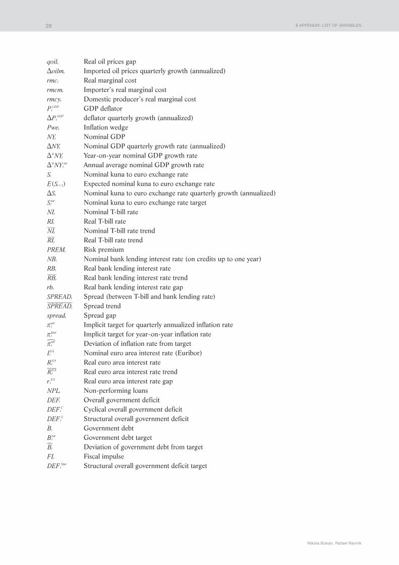
8 APPENDIx: LIST OF VARIABLES
Nikola Bokan, Rafael Ravnik
28
qoilt Real oil prices gapoilmtD Imported oil prices quarterly growth (annualized)rmct Real marginal costrmcmt Importer’s real marginal costrmcyt Domestic producer’s real marginal costPtGDP GDP deflatorPtGDPD deflator quarterly growth (annualized)
Pwet Inflation wedgeNYt Nominal GDPNYtD Nominal GDP quarterly growth rate (annualized)NYt4D Year-on-year nominal GDP growth rateNYt
an4D Annual average nominal GDP growth rateSt Nominal kuna to euro exchange rate( )E St 1+ Expected nominal kuna to euro exchange rateStD Nominal kuna to euro exchange rate quarterly growth (annualized)Sttar Nominal kuna to euro exchange rate targetNIt Nominal T-bill rateRIt Real T-bill rateNIt Nominal T-bill rate trendRIt Real T-bill rate trendPREMt Risk premiumNBt Nominal bank lending interest rate (on credits up to one year)RBt Real bank lending interest rateRBt Real bank lending interest rate trendrbt Real bank lending interest rate gapSPREADt Spread (between T-bill and bank lending rate)SPREADt Spread trendspreadt Spread gapttarr Implicit target for quarterly annualized inflation ratettar4r Implicit target for year-on-year inflation ratettarr\ Deviation of inflation rate from targetItEA Nominal euro area interest rate (Euribor)RtEA Real euro area interest rateRtEA Real euro area interest rate trendrtEA Real euro area interest rate gapNPLt Non-performing loansDEFt Overall government deficitDEFt
C Cyclical overall government deficitDEFt
S Structural overall government deficitBt Government debtBttar Government debt targetBtX Deviation of government debt from targetFIt Fiscal impulseDEFt
Star Structural overall government deficit target

9 APPENDIx: LIST OF EQUATIONS
Quarterly Projection Model for Croatia
29
9 Appendix: List of equations
y Y Yt t t= - r (34)
( )Y Y Y4t t t 1D = - - (35)
Y Y Yt t t4
4D = - - (36)
( )Y Y Y4t t t 1D = - - (37)
( )Y Y Y1t Y SS Y t Y1 ta a fD D D D= + - +D D D- (38)
ad AD ADt t t= - (39)
( )AD AD AD4t t t 1D = - - (40)
AD AD ADt t t4
4D = - - (41)
AD AD AD4t t t 1D = - -^ h (42)
( )ad x dd1t ad t ad t adta a f= + - + (43)
( )AD X DD1t ad t ad t adta a fD D D= + - + (44)
( )4ad ad adt t t 1f f fD = - - (45)
ad m yt ym t yy t yta a f= + + (46)
AD M Yt ym t yy t yta a fD D D= + + (47)
( )4y y y 1t t tf f fD = - - (48)
dd DD DDt t t= - (49)
( )DD DD DD4t t t 1D = - - (50)
DD DD DDt t t4
4D = - - (51)
DD DD DD4t t t 1D = - -^ h (52)
( ) ( )dd E dd dd rb FI1t dde t dde t ddr t ddf t dd1 1 ta a a a f= + - - + ++ - (53)
( ) ( )E dd dd dd1t dde t dde t1 1 1 1 1a a= + -+ + - (54)
x X Xt t t= - (55)
( )X X X4t t t 1D = - - (56)
X X Xt t t4
4D = - - (57)

9 APPENDIx: LIST OF EQUATIONS
Nikola Bokan, Rafael Ravnik
30
X X X4t t t 1D = - -^ h (58)
( )X X X1t Y SS Y t X1 ta aa fD D D D= + - +D D D- (59)
x y zt tEA
xz t xta f= + + (60)
m M Mt t t= - (61)
( )M M M4t t t 1D = - - (62)
M M Mt t t4
4D = - - (63)
M M M4t t t 1D = - -^ h (64)
( )M M M1t Y SS Y t M1 ta a fD D D D= + - +D D D- (65)
( )m y rmcm rmcyt t my t t mta f= - - + (66)
( )y y y y y41
tan
t t t t1 2 3= + + +- - - (67)
( )dd dd dd dd dd41
tan
t t t t1 2 3= + + +- - - (68)
Z S P Pt tEA
t= + - (69)
z Z Zt t t= - (70)
( )Z Z Z4t t t 1D = - - (71)
Z Z Z4t t t 1D = - -^ h (72)
( )Z Z Z1t Z t Z SS Z1 ti i fD D D= + - +D D D- (73)
( )P P4t t t 1r = - - (74)
( ) ( )P P41
t t t t t t t4
1 2 3 4r r r r r= + + + = -- - - - (75)
( ) ( )E oilm rmc1t oil t t oil t rmc t1 1 1 1 tr i i r i r i i fD= - - + + + +r r r r r r+ - (76)
( ) ( )E 1t e t e t1 1 1r i r i r= + -r r+ + - (77)
( ) ( )E 1t e t e t14
44
14r i r i r= + -r r+ + - (78)
QOIL OIL Pt t tEA= - (79)
QOIL QOIL qoilt t t= + (80)
qoil qoilt qoil t qoil1 ti f= +- (81)
( )OIL OIL OIL4t t t 1D = - - (82)

9 APPENDIx: LIST OF EQUATIONS
Quarterly Projection Model for Croatia
31
( )QOIL QOIL QOIL1t QOIL t QOIL SS QOIL1 ti i fD D D= + - +D D D- (83)
oilm OIL S QOIL Zt t t t tD D D D D= + - - (84)
( )rmc rmcy rmcm qoilt rmcy t rmcm rmcqo t rmcqo ti i i i= + - + (85)
rmcy yt t= (86)
rmcm zt t= V (87)
( )P P P4tGDP
tGDP
tGDP1= - - (88)
P PwetGDP
t trD = + (89)
( )Pwe Pwe Pwe1t Pwe t Pwe SS Pwe1 ti i f= + - +- (90)
NY P Yt tGDP
t= + (91)
( )NY NY NY4t t t 1D = - - (92)
NY NY NYt t t4
4D = - - (93)
( )NY NY NY NY NY41
tan
t t t t4 4 4
14
24
3D D D D D= + + +- - - (94)
( )P P4tEA
tEA
tEA1r = - - (95)
( )( ( ( ) ) )NI NI I E S S PREM1t NI t NI tEA
t t t NI1 1 tz z f= + - + - + +- + (96)
( ) ( )E S S S1t ES t ES t1 1 1z z= + -+ + - (97)
( )RI R E Z PREMt SSEA
t t1D= + ++ (98)
( )PREM PREM PREM1t PREM t PREM SS PREM1 tz z f= + - +- (99)
PREM PREM premt t t= + (100)
prem DEF DEF DEF DEFDEF prem4t prdef
tS
tS
tS
tS
SSS
prlag t prem1 2 3
1 tz z f= + + +- + +- - -
-b l (101)
RI NIt t ttarr= - (102)
( )RI NI Et t t 1r= - + (103)
( )RB NB Et t t 1r= - + (104)
rb RB RBt t t= - (105)
RB SPREAD RIt t t= + (106)
( ) ( )NB NB NI SPREAD1t NB t NB t t NB1 tz z f= - + + +- (107)
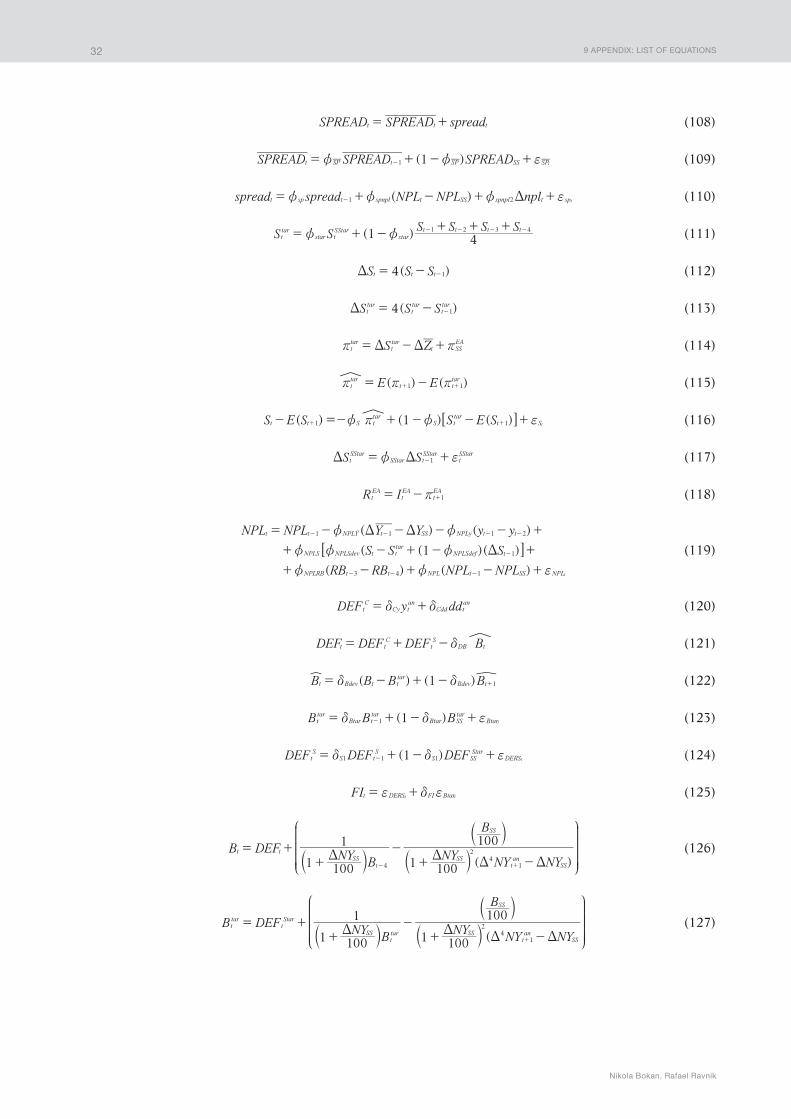
9 APPENDIx: LIST OF EQUATIONS
Nikola Bokan, Rafael Ravnik
32
SPREAD SPREAD spreadt t t= + (108)
( )SPREAD SPREAD SPREAD1t SP t SP SS SP1 tz z f= + - +- (109)
( )spread spread NPL NPL nplt sp t spnpl t SS spnpl t sp1 2 tz z z fD= + - + +- (110)
( )S SS S S S
1 4ttar
star tSStar
start t t t1 2 3 4z z= + -+ + +- - - - (111)
( )S S S4t t t 1D = - - (112)
( )S S S4ttar
ttar
ttar1D = - - (113)
S Zttar
ttar
t SSEAr rD D= - + (114)
( ) ( )E Ettar
t ttar
1 1r r r= -+ +% (115)
( ) ( ) ( )S E S S E S1t t S ttar
S ttar
t S1 1 tz r z f- =- + - - ++ +6 @% (116)
S StSStar
SStar tSStar
tSStar
1z fD D= +- (117)
R ItEA
tEA
tEA1r= - + (118)
( ) ( )
( ( )( )
( ) ( )
NPL NPL Y Y y y
S S S
RB RB NPL NPL
1
t t NPLY t SS NPLy t t
NPLS NPLSdev t ttar
NPLSdef t
NPLRB t t NPL t SS NPL
1 1 1 2
1
3 4 1 t
z z
z z z
z z f
D D
D
= - - - - +
+ - + - +
+ - + - +
- - - -
-
- - -
r
6 @ (119)
DEF y ddtC
Cy tan
Cdd tand d= + (120)
DEF DEF DEF Bt tC
tS
DB td= + - % (121)
( ) ( )B B B B1t Bdev t ttar
Bdev t 1d d= - + - +X \ (122)
( )B B B1ttar
Btar ttar
Btar SStar
Btar1 td d f= + - +- (123)
( )DEF DEF DEF1tS
S tS
S SSStar
DERS1 1 1 td d f= + - +- (124)
FIt DERS FI Btart tf d f= + (125)
( )
B DEFNY
BNY
NY NY
B
1 100
1
1 100
100t t
SSt
SStan
SS
SS
4
24
1D D
D D= +
+-
+ -- +
J
L
KKKKKKKKb bb N
P
OOOOOOOOl ll
(126)
(
B DEFNY
BNY
NY NY
B
1 100
1
1 100
100ttar
tStar
SSttar SS
tan
SS
SS
24
1D D
D D= +
+-
+ -+
J
L
KKKKKKKKb bb N
P
OOOOOOOOl ll
(127)
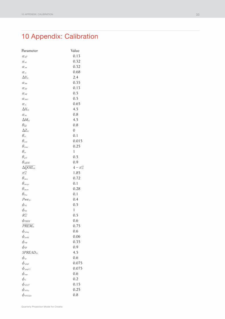
10 APPENDIx: CALIBRATION
Quarterly Projection Model for Croatia
33
10 Appendix: Calibration
Parameter ValueYaD 0.13ada 0.32yma 0.32yya 0.68YSSD 2.4ddea 0.35ddra 0.13ddfa 0.5dde1a 0.5xza 0.65XSSD 4.5mya 0.8MSSD 4.5ZiD 0.8ZSSD 01ir 0.1oilir 0.015rmcir 0.25eir 1qoili 0.5QOILiD 0.9QOILSSD 4 SS
ESr-
SSEAr 1.85rmcyi 0.72rmcqoi 0.1rmcmi 0.28Pwei 0.1PweSS 0.4NIz 0.5ESz 1RSSEA 0.5PREMz 0.6PREMSS 0.75prlagz 0.6prdefz 0.06NBz 0.35SPz 0.9SPREADSS 4.5spz 0.6spnplz 0.075spnpl 2z 0.075starz 0.6Sz 0.2NPLYz 0.15NPLyz 0.25NPLSdevz 0.8

10 APPENDIx: CALIBRATION
Nikola Bokan, Rafael Ravnik
34
NPLSz 0.7NPLRBz 0.2NPLz 0.04NPLSS 10Cyd –0.49Cddd –0.43DBd 0.05Bdevd 0.3Btard 0.995BSStar 70DEFSS
Star 2.9S1d 0.95FId 0.1NYSSD Y PweSS SS SSrD + +
SSr ZSSEA
SSr D-

11 APPENDIx: FIGURES AND TABLES
Quarterly Projection Model for Croatia
35
Sources: Model output.
Figure 4 Exchange rate shock
–0.10
–0.08
–0.06
–0.04
–0.02
0.00
0.02
0.04
0.06
0.08
0.10
0.12
Domestic demand gap Output gap Foreign output gap
CPI inflation (p.p.) Output gap (p.p.)
–0.50
–0.40
–0.30
–0.20
–0.10
0.00
0.10
0.20
0.30
0.40
0.50
0 4 8 12 16 20 24 28 32 36 0 4 8 12 16 20 24 28 32 36
Inflation Inflation targetInflation expectations Foreign inflation
Imports and exports gap (p.p.) HRK/EUR exchange rate levels (p.p.)
–0.10
–0.05
0.00
0.05
0.10
0.15
0.20
Exports gap Net exports Imports gap
–0.20
0.00
0.20
0.40
0.60
0.80
1.00
1.20
Nominal exchange rate Nominal exchange rate expectationsNominal exchange rate target
0 4 8 12 16 20 24 28 32 360 4 8 12 16 20 24 28 32 36
Nominal interest rate (p.p.) Real monetary conditions index (p.p.)
–0.60
–0.50
–0.40
–0.30
–0.20
–0.10
0.00
0.10
0.20
0.30
Nominal T-bill rate Risk premium Spread
–0.20
0.00
0.20
0.40
0.60
0.80
1.00
1.20
1.40
Real interest rate gap NPLs Real exchange rate gap
0 4 8 12 16 20 24 28 32 360 4 8 12 16 20 24 28 32 36
Government deficit (p.p.) Government debt (p.p.)
0 4 8 12 16 20 24 28 32 36–0.04
–0.03
–0.02
–0.01
0.00
0.01
0.02
0.03
0.04
Deficit Structural deficit
–0.15
–0.10
–0.05
0.00
0.05
0.10
0.15
0.20
Public debt Public debt target
0 4 8 12 16 20 24 28 32 36
11 Appendix: Figures and tables

11 APPENDIx: FIGURES AND TABLES
Nikola Bokan, Rafael Ravnik
36
Sources: Model output.
Figure 5 Shock to the exchange rate steady state
Domestic demand gap Output gap Foreign output gap
CPI inflation (p.p.) Output gap (p.p.)
0 4 8 12 16 20 24 28 32 36 0 4 8 12 16 20 24 28 32 36
Inflation Inflation targetInflation expectations Foreign inflation
Imports and exports gap (p.p.) HRK/EUR exchange rate levels (p.p.)
Exports gap Net exports Imports gap Nominal exchange rate Nominal exchange rate expectationsNominal exchange rate target
0 4 8 12 16 20 24 28 32 360 4 8 12 16 20 24 28 32 36
Nominal interest rate (p.p.) Real monetary conditions index (p.p.)
Nominal T-bill rate Risk premium Spread Real interest rate gap NPLs Real exchange rate gap
0 4 8 12 16 20 24 28 32 360 4 8 12 16 20 24 28 32 36
Government deficit (p.p.) Government debt (p.p.)
0 4 8 12 16 20 24 28 32 36
Deficit Structural deficit Public debt Public debt target
0 4 8 12 16 20 24 28 32 36
–0.50
0.00
0.50
1.00
1.50
2.00
2.50
3.00
–0.10
–0.05
0.00
0.05
0.10
0.15
0.20
0.25
–0.10
–0.05
0.00
0.05
0.10
0.15
0.20
0.25
0.00
0.20
0.40
0.60
0.80
1.00
1.20
1.40
0.00
0.02
0.04
0.06
0.08
0.10
0.12
0.14
0.16
–0.60
–0.40
–0.20
0.00
0.20
0.40
0.60
–0.10
–0.05
0.00
0.05
0.10
0.15
–0.80
–0.70
–0.60
–0.50
–0.40
–0.30
–0.20
–0.10
0.00
0.10

11 APPENDIx: FIGURES AND TABLES
Quarterly Projection Model for Croatia
37
Sources: Model output.
Figure 6 Risk premium shock
Domestic demand gap Output gap Foreign output gap
CPI inflation (p.p.) Output gap (p.p.)
0 4 8 12 16 20 24 28 32 36 0 4 8 12 16 20 24 28 32 36
Inflation Inflation targetInflation expectations Foreign inflation
Imports and exports gap (p.p.) HRK/EUR exchange rate levels (p.p.)
Exports gap Net exports Imports gap Nominal exchange rate Nominal exchange rate expectationsNominal exchange rate target
0 4 8 12 16 20 24 28 32 360 4 8 12 16 20 24 28 32 36
Nominal interest rate (p.p.) Real monetary conditions index (p.p.)
Nominal T-bill rate Risk premium Spread Real interest rate gap NPLs Real exchange rate gap
0 4 8 12 16 20 24 28 32 360 4 8 12 16 20 24 28 32 36
Government deficit (p.p.) Government debt (p.p.)
0 4 8 12 16 20 24 28 32 36
Deficit Structural deficit Public debt Public debt target
0 4 8 12 16 20 24 28 32 36
–0.07
–0.06
–0.05
–0.04
–0.03
–0.02
–0.01
0.00
0.01
0.02
0.03
0.04
–0.30
–0.25
–0.20
–0.15
–0.10
–0.05
0.00
0.05
–0.30
–0.20
–0.10
0.00
0.10
0.20
0.30
0.40
–0.02
–0.01
–0.01
0.00
0.01
0.01
0.02
0.02
0.03
–0.20
0.00
0.20
0.40
0.60
0.80
1.00
1.20
–0.10
–0.05
0.00
0.05
0.10
0.15
0.20
0.25
0.30
0.35
0.40
0.45
–0.04
–0.02
0.00
0.02
0.04
0.06
0.08
0.10
0.12
0.14
0.16
0.00
0.05
0.10
0.15
0.20
0.25
0.30
0.35
0.40
0.45
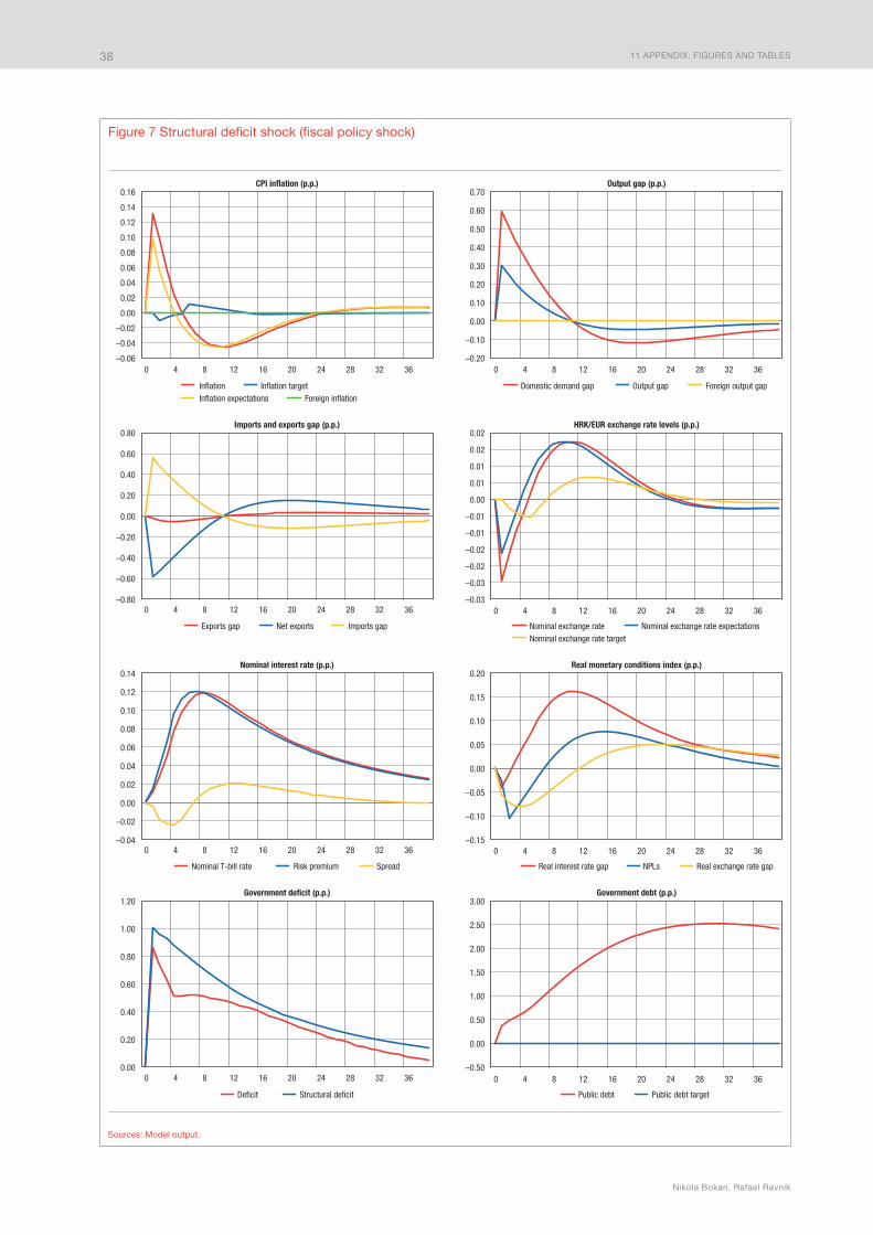
11 APPENDIx: FIGURES AND TABLES
Nikola Bokan, Rafael Ravnik
38
Sources: Model output.
Figure 7 Structural deficit shock (fiscal policy shock)
Domestic demand gap Output gap Foreign output gap
CPI inflation (p.p.) Output gap (p.p.)
0 4 8 12 16 20 24 28 32 36 0 4 8 12 16 20 24 28 32 36
Inflation Inflation targetInflation expectations Foreign inflation
Imports and exports gap (p.p.) HRK/EUR exchange rate levels (p.p.)
Exports gap Net exports Imports gap Nominal exchange rate Nominal exchange rate expectationsNominal exchange rate target
0 4 8 12 16 20 24 28 32 360 4 8 12 16 20 24 28 32 36
Nominal interest rate (p.p.) Real monetary conditions index (p.p.)
Nominal T-bill rate Risk premium Spread Real interest rate gap NPLs Real exchange rate gap
0 4 8 12 16 20 24 28 32 360 4 8 12 16 20 24 28 32 36
Government deficit (p.p.) Government debt (p.p.)
0 4 8 12 16 20 24 28 32 36
Deficit Structural deficit Public debt Public debt target
0 4 8 12 16 20 24 28 32 36
–0.06
–0.04
–0.02
0.00
0.02
0.04
0.06
0.08
0.10
0.12
0.14
0.16
–0.20
–0.10
0.00
0.10
0.20
0.30
0.40
0.50
0.60
0.70
–0.80
–0.60
–0.40
–0.20
0.00
0.20
0.40
0.60
0.80
–0.03
–0.03
–0.02
–0.02
–0.01
–0.01
0.00
0.01
0.01
0.02
0.02
–0.04
–0.02
0.00
0.02
0.04
0.06
0.08
0.10
0.12
0.14
–0.15
–0.10
–0.05
0.00
0.05
0.10
0.15
0.20
0.00
0.20
0.40
0.60
0.80
1.00
1.20
–0.50
0.00
0.50
1.00
1.50
2.00
2.50
3.00

11 APPENDIx: FIGURES AND TABLES
Quarterly Projection Model for Croatia
39
Sources: Model output.
Figure 8 Foreign interest rate shock
Domestic demand gap Output gap Foreign output gap
CPI inflation (p.p.) Output gap (p.p.)
0 4 8 12 16 20 24 28 32 36 0 4 8 12 16 20 24 28 32 36
Inflation Inflation targetInflation expectations Foreign inflation
Imports and exports gap (p.p.) HRK/EUR exchange rate levels (p.p.)
Exports gap Net exports Imports gap Nominal exchange rate Nominal exchange rate expectationsNominal exchange rate target
0 4 8 12 16 20 24 28 32 360 4 8 12 16 20 24 28 32 36
Nominal interest rate (p.p.) Real monetary conditions index (p.p.)
Nominal T-bill rate Risk premium Spread Real interest rate gap NPLs Real exchange rate gap
0 4 8 12 16 20 24 28 32 360 4 8 12 16 20 24 28 32 36
Government deficit (p.p.) Government debt (p.p.)
0 4 8 12 16 20 24 28 32 36
Deficit Structural deficit Public debt Public debt target
0 4 8 12 16 20 24 28 32 36
–0.08
–0.06
–0.04
–0.02
0.00
0.02
0.04
–0.40
–0.35
–0.30
–0.25
–0.20
–0.15
–0.10
–0.05
0.00
0.05
–0.40
–0.30
–0.20
–0.10
0.00
0.10
0.20
0.30
0.40
0.50
–0.02
–0.01
–0.01
0.00
0.01
0.01
0.02
0.02
0.03
0.03
–0.10
0.00
0.10
0.20
0.30
0.40
0.50
0.60
0.70
–0.10
0.00
0.10
0.20
0.30
0.40
0.50
0.60
–0.05
0.00
0.05
0.10
0.15
0.20
–0.10
0.00
0.10
0.20
0.30
0.40
0.50
0.60

11 APPENDIx: FIGURES AND TABLES
Nikola Bokan, Rafael Ravnik
40
Sources: Model output.
Figure 9 Foreign inflation shock
Domestic demand gap Output gap Foreign output gap
CPI inflation (p.p.) Output gap (p.p.)
0 4 8 12 16 20 24 28 32 36 0 4 8 12 16 20 24 28 32 36
Inflation Inflation targetInflation expectations Foreign inflation
Imports and exports gap (p.p.) HRK/EUR exchange rate levels (p.p.)
Exports gap Net exports Imports gap Nominal exchange rate Nominal exchange rate expectationsNominal exchange rate target
0 4 8 12 16 20 24 28 32 360 4 8 12 16 20 24 28 32 36
Nominal interest rate (p.p.) Real monetary conditions index (p.p.)
Nominal T-bill rate Risk premium Spread Real interest rate gap NPLs Real exchange rate gap
0 4 8 12 16 20 24 28 32 360 4 8 12 16 20 24 28 32 36
Government deficit (p.p.) Government debt (p.p.)
0 4 8 12 16 20 24 28 32 36
Deficit Structural deficit Public debt Public debt target
0 4 8 12 16 20 24 28 32 36
–0.20
0.00
0.20
0.40
0.60
0.80
1.00
1.20
0.00
0.05
0.10
0.15
0.20
0.25
0.30
0.35
0.40
0.45
–0.50
–0.40
–0.30
–0.20
–0.10
0.00
0.10
0.20
0.30
0.40
0.50
–0.20
–0.15
–0.10
–0.05
0.00
0.05
–0.16
–0.14
–0.12
–0.10
–0.08
–0.06
–0.04
–0.02
0.00
0.02
0.04
–0.60
–0.50
–0.40
–0.30
–0.20
–0.10
0.00
0.10
–0.15
–0.10
–0.05
0.00
0.05
0.10
0.15
–1.20
–1.00
–0.80
–0.60
–0.40
–0.20
0.00

11 APPENDIx: FIGURES AND TABLES
Quarterly Projection Model for Croatia
41
Sources: Model output.
Figure 10 Foreign output gap shock
Domestic demand gap Output gap Foreign output gap
CPI inflation (p.p.) Output gap (p.p.)
0 4 8 12 16 20 24 28 32 36 0 4 8 12 16 20 24 28 32 36
Inflation Inflation targetInflation expectations Foreign inflation
Imports and exports gap (p.p.) HRK/EUR exchange rate levels (p.p.)
Exports gap Net exports Imports gap Nominal exchange rate Nominal exchange rate expectationsNominal exchange rate target
0 4 8 12 16 20 24 28 32 360 4 8 12 16 20 24 28 32 36
Nominal interest rate (p.p.) Real monetary conditions index (p.p.)
Nominal T-bill rate Risk premium Spread Real interest rate gap NPLs Real exchange rate gap
0 4 8 12 16 20 24 28 32 360 4 8 12 16 20 24 28 32 36
Government deficit (p.p.) Government debt (p.p.)
0 4 8 12 16 20 24 28 32 36
Deficit Structural deficit Public debt Public debt target
0 4 8 12 16 20 24 28 32 36
–0.04
–0.02
0.00
0.02
0.04
0.06
0.08
0.10
0.12
–0.20
0.00
0.20
0.40
0.60
0.80
1.00
1.20
–0.20
0.00
0.20
0.40
0.60
0.80
1.00
1.20
–0.03
–0.02
–0.02
–0.01
–0.01
0.00
0.01
0.01
0.02
–0.03
–0.02
–0.02
–0.01
–0.01
0.00
0.01
0.01
–0.10
–0.08
–0.06
–0.04
–0.02
0.00
0.02
0.04
–0.07
–0.06
–0.05
–0.04
–0.03
–0.02
–0.01
0.00
0.01
0.02
0.03
–0.25
–0.20
–0.15
–0.10
–0.05
0.00
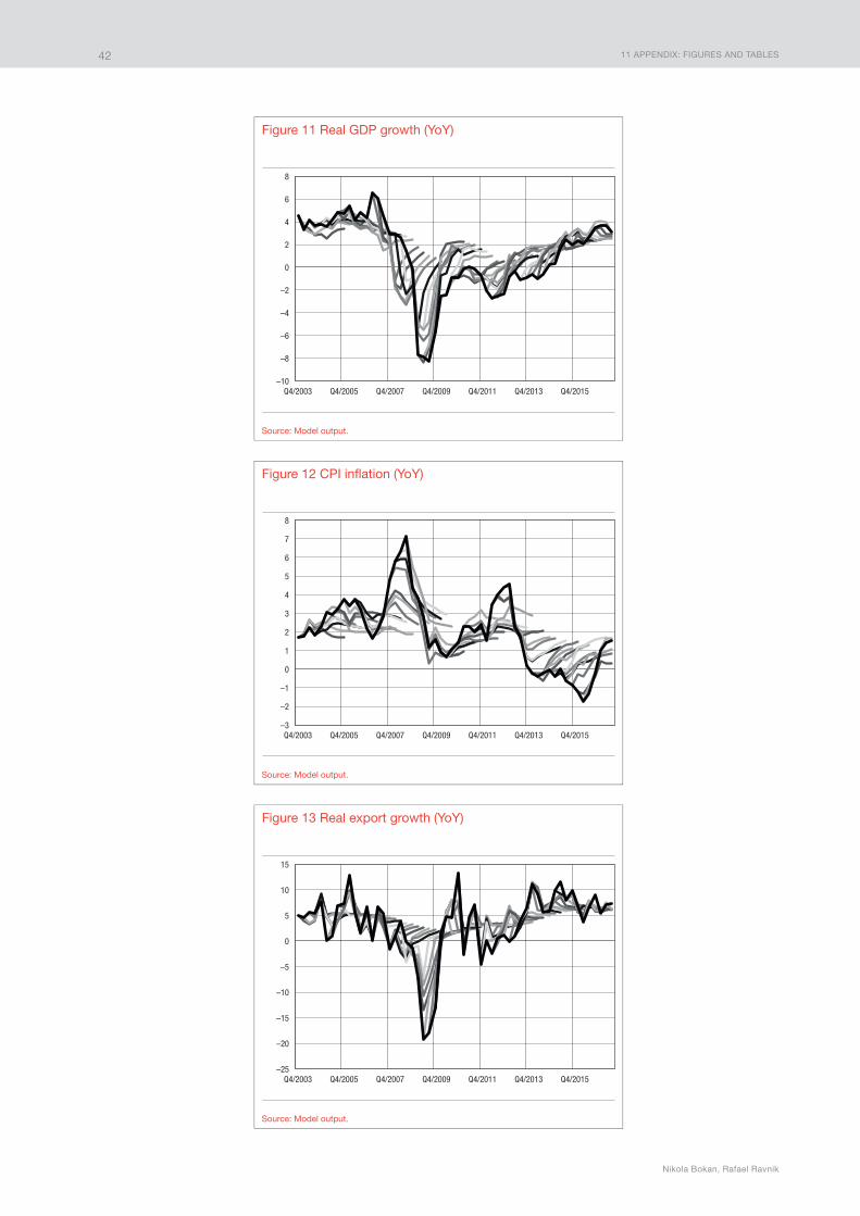
11 APPENDIx: FIGURES AND TABLES
Nikola Bokan, Rafael Ravnik
42
Source: Model output.
Figure 11 Real GDP growth (YoY)
–10
–8
–6
–4
–2
0
2
4
6
8
Q4/2003 Q4/2005 Q4/2007 Q4/2009 Q4/2011 Q4/2013 Q4/2015
Source: Model output.
Figure 12 CPI inflation (YoY)
Q4/2003 Q4/2005 Q4/2007 Q4/2009 Q4/2011 Q4/2013 Q4/2015–3
–2
–1
0
1
2
3
4
5
6
7
8
Source: Model output.
Figure 13 Real export growth (YoY)
Q4/2003 Q4/2005 Q4/2007 Q4/2009 Q4/2011 Q4/2013 Q4/2015–25
–20
–15
–10
–5
0
5
10
15

11 APPENDIx: FIGURES AND TABLES
Quarterly Projection Model for Croatia
43
Source: Model output.
Figure 14 Real imports growth (YoY)
Q4/2003 Q4/2005 Q4/2007 Q4/2009 Q4/2011 Q4/2013 Q4/2015–30
–25
–20
–15
–10
–5
0
5
10
15
20
Source: Model output.
Figure 15 Real exchange rate
Q4/2003 Q4/2005 Q4/2007 Q4/2009 Q4/2011 Q4/2013 Q4/2015196
198
200
202
204
206
208
210
Source: Model output.
Figure 16 Nominal T-bill rate
Q4/2003 Q4/2005 Q4/2007 Q4/2009 Q4/2011 Q4/2013 Q4/20150
1
2
3
4
5
6
7
8
9
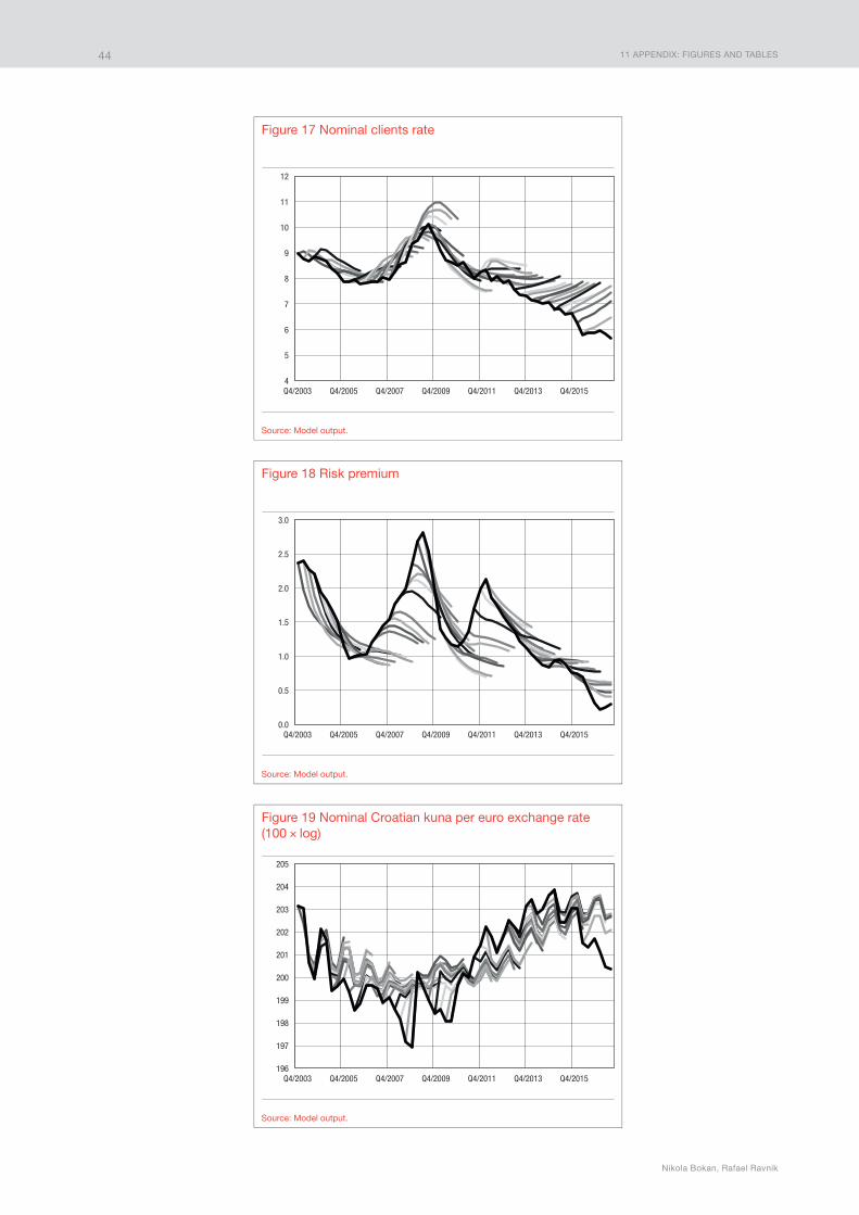
11 APPENDIx: FIGURES AND TABLES
Nikola Bokan, Rafael Ravnik
44
Source: Model output.
Figure 17 Nominal clients rate
Q4/2003 Q4/2005 Q4/2007 Q4/2009 Q4/2011 Q4/2013 Q4/20154
5
6
7
8
9
10
11
12
Source: Model output.
Figure 18 Risk premium
Q4/2003 Q4/2005 Q4/2007 Q4/2009 Q4/2011 Q4/2013 Q4/20150.0
0.5
1.0
1.5
2.0
2.5
3.0
Source: Model output.
Figure 19 Nominal Croatian kuna per euro exchange rate (100 × log)
Q4/2003 Q4/2005 Q4/2007 Q4/2009 Q4/2011 Q4/2013 Q4/2015196
197
198
199
200
201
202
203
204
205

11 APPENDIx: FIGURES AND TABLES
Quarterly Projection Model for Croatia
45
Source: CNB.
Figure 20 Credit default swap for 5-year government bond of the Republic of Croatia and model estimate of risk premium (standardized values)
–2.5
–2.0
–1.5
–1.0
–0.5
0.0
0.5
1.0
1.5
2.0
2.5
3.0
Q1/2007 Q1/2009 Q1/2011 Q1/2013 Q1/2015
Risk premium CDS
Table 1 Relative Root Mean Squared Errors (RMSEs) for in-sample forecasts
Q1 Q2 Q3 Q4 Q5 Q6 Q7 Q8
Nominal HRK per EUR exchange 0.90 0.70 0.81 0.90 0.81 0.75 0.80 0.80
GDP growth YoY 0.89 0.74 0.64 0.59 0.59 0.61 0.64 0.67
GDP growth QoQ 0.82 0.71 0.63 0.78 0.72 0.68 0.72 0.69
CPI inflation (YoY) 0.57 0.52 0.51 0.52 0.58 0.64 0.70 0.72
CPI inflation (QoQ) 0.71 0.79 0.70 0.67 0.73 0.71 0.75 0.76
Real exports growth (YoY) 0.51 0.43 0.42 0.41 0.63 0.63 0.64 0.66
Real imports growth (YoY) 0.62 0.49 0.41 0.37 0.50 0.55 0.60 0.64
GDP gap 1.12 0.97 0.86 0.80 0.75 0.70 0.68 0.67
Real exchange rate 1.23 0.94 0.81 0.76 0.73 0.73 0.75 0.76
Real exchange rate gap 1.34 1.06 0.93 0.84 0.78 0.75 0.76 0.75
Nominal T-bill rate 1.01 0.86 0.71 0.66 0.63 0.66 0.66 0.69
Nominal clients rate 1.14 1.02 0.91 0.85 0.81 0.79 0.78 0.76
Real clients rate gap 1.01 0.92 0.82 0.75 0.70 0.66 0.64 0.63
Risk premium 0.96 0.79 0.69 0.68 0.70 0.74 0.76 0.79
Note: The values shown are RMSEs of the model forecast relative to the respective random walk forecast.Source: Model output.


The following Surveys have been published
No. Date Title Author(s)
S-1 March 2000 Banking Sector Problems: Causes, Solutions and Consequences Ljubinko Jankov
S-2 April 2000 Banking System in 1998
S-3 December 2000The Lending Policies of Croatian Banks: Results of the Second CNB Bank Interview Project
Evan Kraft with Hrvoje Dolenec, Mladen Duliba, Michael Faulend, Tomislav Galac, Vedran Šošić and Mladen Mirko Tepuš
S-4 December 2000 What Has Been the Impact of Foreign Banks in CroatiaTomislav Galac and Evan Kraft
S-5 September 2001 Currency Crises: Theoretical and Empirical Overview of the 1990sAnte Babić and Ante Žigman
S-6 April 2002 An Analysis of the Operation of Building Societies in the Republic of Croatia Mladen Mirko Tepuš
S-7 April 2002 Ten Years of Transition Central Banking in the CEE and the BalticsWarren Coats and Marko Škreb
S-8 May 2002Fiscal Consolidation, External Competitiveness and Monetary Policy: A Reply to the WIIW
Evan Kraft Tihomir Stučka
S-9 November 2004 Survey and Analysis of Foreign Direct Investment in the Republic of Croatia Alen Škudar
S-10 February 2005 Does Croatia Need Risk-Based Deposit Insurance Premia? Tomislav Galac
S-11 February 2005 How Can Croatia’s Deposit Insurance System Be Improved? Michael Faulend and Evan Kraft
S-12 April 2005 An Analysis of Housing Finance Models in the Republic of Croatia Mladen Mirko Tepuš
S-13 July 2005EU Criteria with Special Emphasis on the Economic Convergence Criteria – Where is Croatia?
Michael Faulend, Davor Lončarek, Ivana Curavić and Ana Šabić
S-14 December 2005Results of the Third CNB Bank Survey: Croatian Banking in the Consolidation and Market Positioning Stage, 2000 – 2002
Tomislav Galac
S-15 November 2008 Results of the Fifth CNB Bank SurveyLana Ivičić, Mirna Dumičić, Ante Burić, Ivan Huljak
S-16 December 2008 Results of the Fourth CNB Bank Survey Tomislav Galac and Lana Dukić
S-17 September 2014 Framework for Monitoring Macroeconomic Imbalances in the European Union – Significance for Croatia Mislav Brkić and Ana Šabić
S-18 August 2015 A Brief Introduction to the World of Macroprudential Policy Mirna Dumičić
S-19 October 2015Features of the Labour Market and Wage Setting in Croatia: Firms Survey Results
Marina Kunovac and Andreja Pufnik
S-20 November 2016 Are Shadow Banks Hiding in Croatia as Well? Mirna Dumičić and Tomislav Ridzak
S-21 December 2016 A Note on Kuna Lending Igor Ljubaj and Suzana Petrović
S-22 July 2017Microeconomic Aspects of Productivity Developments during the Great Recession in Croatia – the CompNet Productivity Module Research Results
Miljana Valdec and Jurica Zrnc
S-23 August 2017Price Competitiveness of the Manufacturing Sector – a Sector Approach Based on Technological Intensity Level
Enes Đozović
S-24 October 2017Exposure of the Private Non-financial Sector to Interest Rate Risk: Analysis of Results of the Survey on Interest Rate Variability
Mate Rosan
S-25 August 2017 CNB Transparency and Monetary Policy Katja Gattin Turkalj and Igor Ljubaj
S-26 October 2017Adoption of the Euro in Croatia: Possible Effects on International Trade and Investments
Maja Bukovšak, Andrijana Ćudina and Nina Pavić
S-27 November 2017Effects of the Adoption of the Euro on Consumer Prices and Inflation Perceptions: An Overview of Experiences and Assessment of the Possible Impact in Croatia
Andreja Pufnik
S-28 November 2017 Can the Adoption of the Euro in Croatia Reduce the Cost of Borrowing? Davor Kunovac and Nina Pavić
S-29 November 2017 Estimating Potential Growth and Output Gap in Croatia Goran Jovičić
S-30 January 2018Is the Euro the Optimum Currency for Croatia: An Assessment Using the Optimum Currency Area Theory
Mislav Brkić and Ana Šabić
S-31 February 2018 Persistence of Euroisation in CroatiaMirna Dumičić, Igor Ljubaj and Ana Martinis
S-32 February 2018 Croatia in Global Value ChainsIvana Vidaković Peruško, Katarina Kovač, Miroslav Jošić
S-33 March 2018Seasonal Adjustment of Time Series and Calendar Influence on Economic Activity
Ante Čobanov

Guidelines to authors
In its periodical publications Working Papers, Surveys and Technical Papers, the Croatian National Bank publishes scien-tific and scholarly papers of the Bank’s employees and other associate contributors.
After the submission, the manuscripts shall be subject to peer review and classification by the Manuscript Review and Classification Committee. The authors shall be informed of the acceptance or rejection of their manuscript for publication within two months following the manuscript submission.
Manuscripts are submitted and published in Croatian and/or English language.
Manuscripts submitted for publication should meet the fol-lowing requirements:
Manuscripts should be submitted via e-mail or optical stor-age media (CD, DVD), accompanied by one printed paper copy. The acceptable text format is Word.
The first page of the manuscript should contain the article title, first and last name of the author and his/her academic degree, name of the institution with which the author is associ-ated, author’s co-workers, and the complete mailing address of the corresponding author to whom a copy of the manuscript with requests for corrections shall be sent.
Additional information, such as acknowledgments, should be incorporate in the text at the end of the introductory section.
The second page should contain the abstract and the key words. The abstract is required to be explicit, descriptive, writ-ten in third person, consisting of not more than 250 words (maximum 1500 characters). The abstract should be followed by maximum 5 key words.
A single line spacing and A4 paper size should be used. The text must not be formatted, apart from applying bold and italic script to certain parts of the text. Titles must be numerated and separated from the text by double-line spacing, without for-matting.
Tables, figures and charts that are a constituent part of the
paper must be well laid out, containing: number, title, units of measurement, legend, data source, and footnotes. The foot-notes referring to tables, figures and charts should be indi-cated by lower-case letters (a,b,c…) placed right below. When the tables, figures and charts are subsequently submitted, it is necessary to mark the places in the text where they should be inserted. They should be numbered in the same sequence as in the text and should be referred to in accordance with that numeration. If the tables and charts were previously inserted in the text from other programs, these databases in the Excel format should also be submitted (charts must contain the cor-responding data series).
The preferred formats for illustrations are EPS or TIFF with explanations in 8 point Helvetica (Ariel, Swiss). The scanned illustration must have 300 dpi resolution for grey scale and full colour illustration, and 600 dpi for lineart (line drawings, diagrams, charts).
Formulae must be legible. Indices and superscript must be explicable. The symbols’ meaning must be given following the equation where they are used for the first time. The equations in the text referred to by the author should be marked by a se-rial number in brackets closer to the right margin.
Notes at the foot of the page (footnotes) should by indicat-ed by Arabic numerals in superscript. They should be brief and written in a smaller font than the rest of the text.
References cited in the text are listed at the last page of the manuscript in the alphabetical order, according to the authors’ last names. References should also include data on the pub-lisher, city and year of publishing.
Publishing Department maintains the right to send back for the author’s revision the accepted manuscript and illustrations that do not meet the above stated requirements.
All contributors who wish to publish their papers are wel-comed to do so by addressing them to the Publishing Depart-ment, following the above stated guidelines.

The Croatian National Bank publications
Croatian National Bank – Annual ReportRegular annual publication surveying annual monetary and general economic developments as well as statistical data.
Croatian National Bank – Semi-annual ReportRegular semi-annual publication surveying semi-annual mon-etary and general economic developments and statistical data.
Banks BulletinPublication providing survey of data on banks.
Croatian National Bank – BulletinRegular monthly publication surveying monthly monetary and general economic developments and monetary statistics.
Croatian National Bank – Working PapersOccasional publication containing shorter scientific papers written by the CNB employees and associate contributors.
Croatian National Bank – SurveysOccasional publication containing scholarly papers written by the CNB employees and associate contributors.
Croatian National Bank – Technical PapersOccasional publication containing papers of informative char-acter written by CNB employees and associate contributors.
The Croatian National Bank also issues other publications such as, for example, numismatic issues, brochures, publica-tions in other media (CD-ROM, DVD), books, monographs and papers of special interest to the CNB as well as proceed-ings of conferences organised or co-organised by the CNB, ed-ucational materials and other similar publications.


ISSN 1334-014x (online)