quasi- and multilevel monte carlo methods for … · bayesian inverse problems in subsurface flow...
TRANSCRIPT
Quasi- and Multilevel Monte Carlo Methods forBayesian Inverse Problems in Subsurface Flow
Aretha Teckentrup
Mathematics Institute, University of Warwick
Joint work with:
Rob Scheichl (Bath), Andrew Stuart (Warwick)
5 February, 2015
A. Teckentrup (WMI) MLMC for Bayesian Inverse Problems 5 February, 2015 1 / 20

Outline
1 Introduction
2 Posterior Expectation as High Dimensional Integration
3 MC, QMC and MLMC
4 Convergence and Complexity
5 Numerical Results
6 Conclusions
A. Teckentrup (WMI) MLMC for Bayesian Inverse Problems 5 February, 2015 2 / 20
Introduction: Model problem
QUATERNARY
MERCIA MUDSTONE
VN-S CALDER
FAULTED VN-S CALDER
N-S CALDER
FAULTED N-S CALDER
DEEP CALDER
FAULTED DEEP CALDER
VN-S ST BEES
FAULTED VN-S ST BEES
N-S ST BEES
FAULTED N-S ST BEES
DEEP ST BEES
FAULTED DEEP ST BEES
BOTTOM NHM
FAULTED BNHM
SHALES + EVAP
BROCKRAM
FAULTED BROCKRAM
COLLYHURST
FAULTED COLLYHURST
CARB LST
FAULTED CARB LST
N-S BVG
FAULTED N-S BVG
UNDIFF BVG
FAULTED UNDIFF BVG
F-H BVG
FAULTED F-H BVG
BLEAWATH BVG
FAULTED BLEAWATH BVG
TOP M-F BVG
FAULTED TOP M-F BVG
N-S LATTERBARROW
DEEP LATTERBARROW
N-S SKIDDAW
DEEP SKIDDAW
GRANITE
FAULTED GRANITE
WASTE VAULTS
CROWN SPACE
EDZ
c©NIREX UK Ltd.
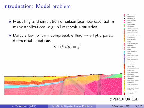
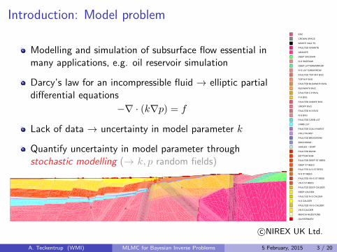
Modelling and simulation of subsurface flow essential inmany applications, e.g. oil reservoir simulation
Darcy’s law for an incompressible fluid → elliptic partialdifferential equations
−∇ · (k∇p) = f
Lack of data → uncertainty in model parameter k
Quantify uncertainty in model parameter throughstochastic modelling (→ k, p random fields)
A. Teckentrup (WMI) MLMC for Bayesian Inverse Problems 5 February, 2015 3 / 20
Introduction: Model problem
QUATERNARY
MERCIA MUDSTONE
VN-S CALDER
FAULTED VN-S CALDER
N-S CALDER
FAULTED N-S CALDER
DEEP CALDER
FAULTED DEEP CALDER
VN-S ST BEES
FAULTED VN-S ST BEES
N-S ST BEES
FAULTED N-S ST BEES
DEEP ST BEES
FAULTED DEEP ST BEES
BOTTOM NHM
FAULTED BNHM
SHALES + EVAP
BROCKRAM
FAULTED BROCKRAM
COLLYHURST
FAULTED COLLYHURST
CARB LST
FAULTED CARB LST
N-S BVG
FAULTED N-S BVG
UNDIFF BVG
FAULTED UNDIFF BVG
F-H BVG
FAULTED F-H BVG
BLEAWATH BVG
FAULTED BLEAWATH BVG
TOP M-F BVG
FAULTED TOP M-F BVG
N-S LATTERBARROW
DEEP LATTERBARROW
N-S SKIDDAW
DEEP SKIDDAW
GRANITE
FAULTED GRANITE
WASTE VAULTS
CROWN SPACE
EDZ
c©NIREX UK Ltd.
Modelling and simulation of subsurface flow essential inmany applications, e.g. oil reservoir simulation
Darcy’s law for an incompressible fluid → elliptic partialdifferential equations
−∇ · (k∇p) = f
Lack of data → uncertainty in model parameter k
Quantify uncertainty in model parameter throughstochastic modelling (→ k, p random fields)
A. Teckentrup (WMI) MLMC for Bayesian Inverse Problems 5 February, 2015 3 / 20
Introduction: Model problem
The end goal is usually to estimate the expected value of a quantityof interest (QoI) φ(p) or φ(k, p).
I point values or local averages of the pressure p
I point values or local averages of the Darcy flow −k∇pI outflow over parts of the boundary
I travel times of contaminant particles
We will work in the Bayesian framework, where we put a priordistribution on k, and obtain a posterior distribution on k byconditioning the prior on observed data.
A. Teckentrup (WMI) MLMC for Bayesian Inverse Problems 5 February, 2015 4 / 20
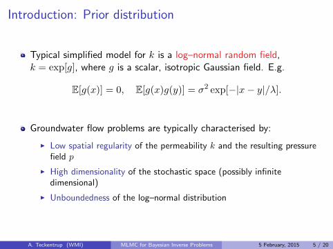
Introduction: Prior distribution
Typical simplified model for k is a log–normal random field,k = exp[g], where g is a scalar, isotropic Gaussian field. E.g.
E[g(x)] = 0, E[g(x)g(y)] = σ2 exp[−|x− y|/λ].
Groundwater flow problems are typically characterised by:
I Low spatial regularity of the permeability k and the resulting pressurefield p
I High dimensionality of the stochastic space (possibly infinitedimensional)
I Unboundedness of the log–normal distribution
A. Teckentrup (WMI) MLMC for Bayesian Inverse Problems 5 February, 2015 5 / 20
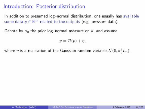
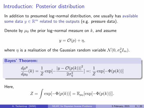
Introduction: Posterior distribution
In addition to presumed log–normal distribution, one usually has availablesome data y ∈ Rm related to the outputs (e.g. pressure data).
Denote by µ0 the prior log–normal measure on k, and assume
y = O(p) + η,
where η is a realisation of the Gaussian random variable N (0, σ2ηIm).
Bayes’ Theorem:
dµy
dµ0(k) =
1
Zexp[−|y −O(p(k))|2
2σ2η] =:
1
Zexp[−Φ(p(k))]
Here,
Z =
∫exp[−Φ(p(k))] = Eµ0 [exp[−Φ(p(k))]].
A. Teckentrup (WMI) MLMC for Bayesian Inverse Problems 5 February, 2015 6 / 20
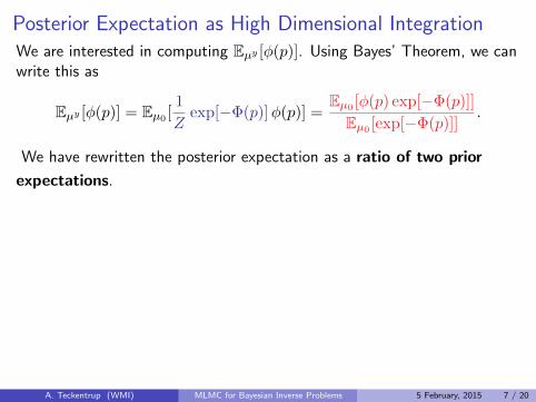
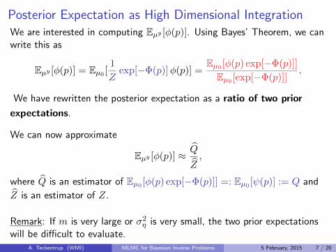
Posterior Expectation as High Dimensional IntegrationWe are interested in computing Eµy [φ(p)]. Using Bayes’ Theorem, we canwrite this as
Eµy [φ(p)] = Eµ0 [1
Zexp[−Φ(p)]φ(p)] =
Eµ0 [φ(p) exp[−Φ(p)]]
Eµ0 [exp[−Φ(p)]].
We have rewritten the posterior expectation as a ratio of two prior
expectations.
We can now approximate
Eµy [φ(p)] ≈ Q
Z,
where Q is an estimator of Eµ0 [φ(p) exp[−Φ(p)]] =: Eµ0 [ψ(p)] := Q and
Z is an estimator of Z.
Remark: If m is very large or σ2η is very small, the two prior expectationswill be difficult to evaluate.
A. Teckentrup (WMI) MLMC for Bayesian Inverse Problems 5 February, 2015 7 / 20
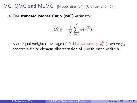
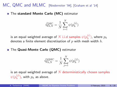
MC, QMC and MLMC [Niederreiter ’94], [Graham et al ’14]
The standard Monte Carlo (MC) estimator
QMCh,N =
1
N
N∑i=1
ψ(p(i)h )
is an equal weighted average of N i.i.d samples ψ(p(i)h ), where ph
denotes a finite element discretisation of p with mesh width h.
The Quasi-Monte Carlo (QMC) estimator
QQMCh,N =
1
N
N∑j=1
ψ(p(j)h )
is an equal weighted average of N deterministically chosen samples
ψ(p(j)h ), with ph as above.
A. Teckentrup (WMI) MLMC for Bayesian Inverse Problems 5 February, 2015 8 / 20
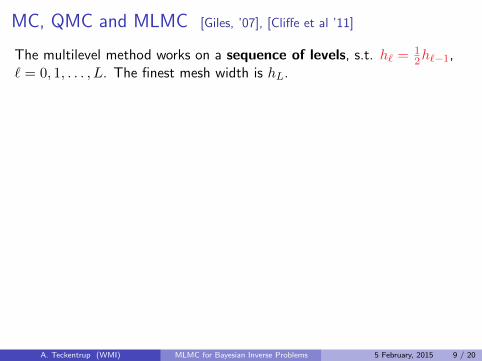
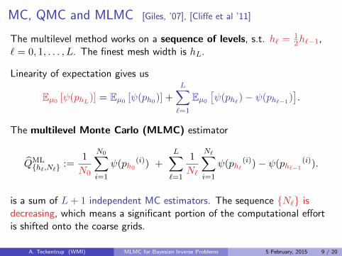
MC, QMC and MLMC [Giles, ’07], [Cliffe et al ’11]
The multilevel method works on a sequence of levels, s.t. h` = 12h`−1,
` = 0, 1, . . . , L. The finest mesh width is hL.
Linearity of expectation gives us
Eµ0 [ψ(phL)] = Eµ0 [ψ(ph0)] +L∑`=1
Eµ0[ψ(ph`)− ψ(ph`−1
)].
The multilevel Monte Carlo (MLMC) estimator
QML{h`,N`} :=
1
N0
N0∑i=1
ψ(ph0(i)) +
L∑`=1
1
N`
N∑i=1
ψ(ph`(i))− ψ(ph`−1
(i)).
is a sum of L+ 1 independent MC estimators. The sequence {N`} isdecreasing, which means a significant portion of the computational effortis shifted onto the coarse grids.
A. Teckentrup (WMI) MLMC for Bayesian Inverse Problems 5 February, 2015 9 / 20
MC, QMC and MLMC [Giles, ’07], [Cliffe et al ’11]
The multilevel method works on a sequence of levels, s.t. h` = 12h`−1,
` = 0, 1, . . . , L. The finest mesh width is hL.
Linearity of expectation gives us
Eµ0 [ψ(phL)] = Eµ0 [ψ(ph0)] +
L∑`=1
Eµ0[ψ(ph`)− ψ(ph`−1
)].
The multilevel Monte Carlo (MLMC) estimator
QML{h`,N`} :=
1
N0
N0∑i=1
ψ(ph0(i)) +
L∑`=1
1
N`
N∑i=1
ψ(ph`(i))− ψ(ph`−1
(i)).
is a sum of L+ 1 independent MC estimators. The sequence {N`} isdecreasing, which means a significant portion of the computational effortis shifted onto the coarse grids.
A. Teckentrup (WMI) MLMC for Bayesian Inverse Problems 5 February, 2015 9 / 20
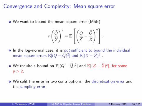
Convergence and Complexity: Mean square error
We want to bound the mean square error (MSE)
e
(Q
Z
)2
= E
(QZ− Q
Z
)2 .
In the log–normal case, it is not sufficient to bound the individualmean square errors E[(Q− Q)2] and E[(Z − Z)2].
We require a bound on E[(Q− Q)2] and E[(Z − Z)p], for somep > 2.
We split the error in two contributions: the discretisation error andthe sampling error.
A. Teckentrup (WMI) MLMC for Bayesian Inverse Problems 5 February, 2015 10 / 20
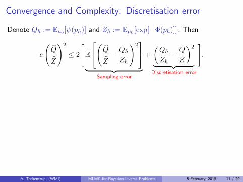
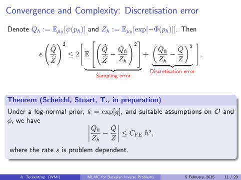
Convergence and Complexity: Discretisation error
Denote Qh := Eµ0 [ψ(ph)] and Zh := Eµ0 [exp[−Φ(ph)]]. Then
e
(Q
Z
)2
≤ 2
[E
(QZ− QhZh
)2
︸ ︷︷ ︸Sampling error
+
(QhZh− Q
Z
)2
︸ ︷︷ ︸Discretisation error
].
Theorem (Scheichl, Stuart, T., in preparation)
Under a log-normal prior, k = exp[g], and suitable assumptions on O andφ, we have ∣∣∣∣QhZh − Q
Z
∣∣∣∣ ≤ CFE hs,
where the rate s is problem dependent.
A. Teckentrup (WMI) MLMC for Bayesian Inverse Problems 5 February, 2015 11 / 20
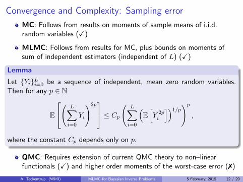
Convergence and Complexity: Sampling error
MC: Follows from results on moments of sample means of i.i.d.random variables (X)
MLMC: Follows from results for MC, plus bounds on moments ofsum of independent estimators (independent of L) (X)
Lemma
Let {Yi}Li=0 be a sequence of independent, mean zero random variables.Then for any p ∈ N
E
( L∑i=0
Yi
)2p ≤ Cp( L∑
i=0
(E[Y 2pi
])1/p)p,
where the constant Cp depends only on p.
QMC: Requires extension of current QMC theory to non–linearfunctionals (X) and higher order moments of the worst-case error (7)
A. Teckentrup (WMI) MLMC for Bayesian Inverse Problems 5 February, 2015 12 / 20
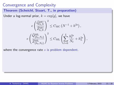
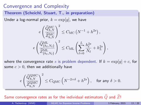
Convergence and ComplexityTheorem (Scheichl, Stuart, T., in preparation)
Under a log-normal prior, k = exp[g], we have
e
(QMCh,N
ZMCh,N
)2
≤ CMC
(N−1 + h2s
),
e
(QML{h`,N`}
ZML{h`,N`}
)2
≤ CML
(L∑`=0
h2s`N`
+ h2sL
),
where the convergence rate s is problem dependent.
If k = exp[g] + c, forsome c > 0, then we additionally have
e
(QQMCh,N
ZQMCh,N
)2
≤ CQMC
(N−2+δ + h2s
), for any δ > 0.
Same convergence rates as for the individual estimators Q and Z!
A. Teckentrup (WMI) MLMC for Bayesian Inverse Problems 5 February, 2015 13 / 20
Convergence and ComplexityTheorem (Scheichl, Stuart, T., in preparation)
Under a log-normal prior, k = exp[g], we have
e
(QMCh,N
ZMCh,N
)2
≤ CMC
(N−1 + h2s
),
e
(QML{h`,N`}
ZML{h`,N`}
)2
≤ CML
(L∑`=0
h2s`N`
+ h2sL
),
where the convergence rate s is problem dependent. If k = exp[g] + c, forsome c > 0, then we additionally have
e
(QQMCh,N
ZQMCh,N
)2
≤ CQMC
(N−2+δ + h2s
), for any δ > 0.
Same convergence rates as for the individual estimators Q and Z!
A. Teckentrup (WMI) MLMC for Bayesian Inverse Problems 5 February, 2015 13 / 20
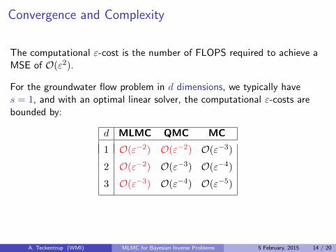
Convergence and Complexity
The computational ε-cost is the number of FLOPS required to achieve aMSE of O(ε2).
For the groundwater flow problem in d dimensions, we typically haves = 1, and with an optimal linear solver, the computational ε-costs arebounded by:
d MLMC QMC MC
1 O(ε−2) O(ε−2) O(ε−3)
2 O(ε−2) O(ε−3) O(ε−4)
3 O(ε−3) O(ε−4) O(ε−5)
A. Teckentrup (WMI) MLMC for Bayesian Inverse Problems 5 February, 2015 14 / 20
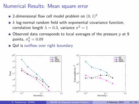
Numerical Results: Mean square error
2-dimensional flow cell model problem on (0, 1)2
k log-normal random field with exponential covariance function,correlation length λ = 0.3, variance σ2 = 1
Observed data corresponds to local averages of the pressure p at 9points, σ2η = 0.09
QoI is outflow over right boundary
A. Teckentrup (WMI) MLMC for Bayesian Inverse Problems 5 February, 2015 15 / 20
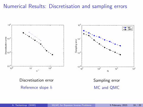
Numerical Results: Discretisation and sampling errors
Discretisation error
Reference slope h
Sampling error
MC and QMC
A. Teckentrup (WMI) MLMC for Bayesian Inverse Problems 5 February, 2015 16 / 20
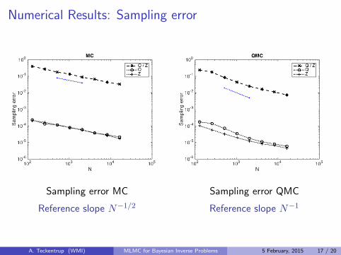
Numerical Results: Sampling error
Sampling error MC
Reference slope N−1/2
Sampling error QMC
Reference slope N−1
A. Teckentrup (WMI) MLMC for Bayesian Inverse Problems 5 February, 2015 17 / 20
Conclusions
Posterior expectations can be written as the ratio of priorexpectations, and in this way approximated using QMC and MLMCmethods.
A convergence and complexity analysis of the resulting estimatorsshowed that the complexity of this approach is the same ascomputing prior expectations.
Numerical investigations confirm the effectiveness of the QMC andMLMC estimators for a typical model problem in subsurface flow.
A. Teckentrup (WMI) MLMC for Bayesian Inverse Problems 5 February, 2015 18 / 20
References I
R. Scheichl, A.M. Stuart, and A.L. Teckentrup.Quasi-Monte Carlo and Multilevel Monte Carlo Methods forComputing Posterior Expectations in Elliptic Inverse Problems.In preparation.
H. Niederreiter.Random Number Generation and quasi-Monte Carlo methods.SIAM, 1994.
I.G. Graham, F.Y. Kuo, J.A. Nicholls, R. Scheichl, Ch. Schwab, andI.H. Sloan.Quasi-Monte Carlo Finite Element methods for Elliptic PDEs withLog-normal Random Coefficients.Numerische Mathematik, (Published online), 2014.
A. Teckentrup (WMI) MLMC for Bayesian Inverse Problems 5 February, 2015 19 / 20
References II
M.B. Giles.Multilevel Monte Carlo path simulation.Opererations Research, 256:981–986, 2008.
K.A. Cliffe, M.B. Giles, R. Scheichl, and A.L. Teckentrup.Multilevel Monte Carlo methods and applications to elliptic PDEs withrandom coefficients.Computing and Visualization in Science, 14:3–15, 2011.
A.L. Teckentrup, R. Scheichl, M.B. Giles, and E. Ullmann.Further analysis of multilevel Monte Carlo methods for elliptic PDEswith random coefficients.Numerische Mathematik, 3(125):569–600, 2013.
A. Teckentrup (WMI) MLMC for Bayesian Inverse Problems 5 February, 2015 20 / 20