quasi-experimental evaluation of reentry programs · 2017-08-21 · reentry services have been...
TRANSCRIPT
QUASI-EXPERIMENTAL EVALUATION OF REENTRY PROGRAMS IN WASHINGTON AND LINN COUNTIES
August 2017
Jason E. Chapman, Ph.D., Michael R. McCart, Ph.D.,1 & Ashli J. Sheidow, Ph.D.
Oregon Social Learning Center
In collaboration with stakeholders from:
Washington County, Oregon,
Linn County, Oregon, &
Oregon Criminal Justice Commission
1 Direct inquiries to Michael R. McCart, Ph.D., Oregon Social Learning Center, 10 Shelton McMurphey Blvd., Eugene, OR 97401; [email protected].

QUASI-EXPERIMENTAL EVALUATION OF REENTRY PROGRAMS 2

QUASI-EXPERIMENTAL EVALUATION OF REENTRY PROGRAMS 3
Table of Contents
List of Tables ............................................................................................................................. 4
List of Figures ............................................................................................................................ 4
Background ................................................................................................................................ 6
Methods ..................................................................................................................................... 9
Evaluation Design and Statistical Method ............................................................................... 9
Sample Description ...............................................................................................................11
Outcomes and Modeling Strategy ..........................................................................................13
Findings ....................................................................................................................................17
Evaluation Question 1: Across counties, did recidivism rates improve in the years following the start of Reentry programming? ..........................................................................17
Evaluation Question 2: Across counties, were recidivism rates lower for those reporting greater use of pre-release Reach-Ins?....................................................................20
Evaluation Question 3: Did Washington and Linn Counties improve more than other counties after Reentry programming? ....................................................................................24
Evaluation Question 4: For Washington and Linn Counties, did recidivism rates improve relative to other counties in the state? ......................................................................32
Reentry Program Effect Size: Preliminary Estimate Based on Reach-In Data .......................36
Conclusion and Recommendations ...........................................................................................37
Appendix 1: Technical Explanation of Evaluation Design and Statistical Analyses ....................38
Appendix 2: Control Variables (Covariates) ...............................................................................44
Modeling Covariates ..............................................................................................................45
Controlled Results: Do Conclusions Change? .......................................................................46
Summary of Controlled Results .............................................................................................48
Appendix 3: Observed Prison Releases and Recidivism Rates by County and Year .................49
QUASI-EXPERIMENTAL EVALUATION OF REENTRY PROGRAMS 4
List of Tables
Table 1. Sample Demographic and Descriptive Information ......................................................11
Table 2. Control Variables (Covariates) Examined in the Reentry Program Evaluation .............44
List of Figures
Figure 1. Statewide Average Recidivism Rates by Year ............................................................14
Figure 2. Washington County Recidivism Rates by Year ..........................................................15
Figure 3. Linn County Recidivism Rates by Year ......................................................................16
Figure 4. Predicted Probability of Arrest Recidivism Across Counties .......................................17
Figure 5. Predicted Probability of Conviction Recidivism Across Counties ................................18
Figure 6. Predicted Probability of Incarceration Recidivism Across Counties ............................19
Figure 7. Predicted Probability of Arrest Recidivism at Low, Average, and High Levels of Pre-Release Prison Reach-Ins ..................................................................................................21
Figure 8. Predicted Probability of Conviction Recidivism at Low, Average, and High Levels of Pre-Release Prison Reach-Ins ...................................................................................22
Figure 9. Predicted Probability of Incarceration Recidivism at Low, Average, and High Levels of Pre-Release Prison Reach-Ins ...................................................................................23
Figure 10. Each County’s Annual Rate Multiplier for Arrest Recidivism (Each County’s Annual Change from Baseline Compared to the Statewide Change from Baseline) ..................25
Figure 11. Each County’s Annual Rate Multiplier for Arrest Recidivism (Each County’s Annual Change from Baseline Compared to the Statewide Change from Baseline), Washington and Linn Counties Identified ..................................................................................26
Figure 12. Each County’s Annual Rate Multiplier for Conviction Recidivism (Each County’s Annual Change from Baseline Compared to the Statewide Change from Baseline), Washington and Linn Counties Identified .................................................................27
Figure 13. Each County’s Annual Rate Multiplier for Incarceration Recidivism (Each County’s Annual Change from Baseline Compared to the Statewide Change from Baseline), Washington and Linn Counties Identified .................................................................28
Figure 14. Each County’s Intervention Period (2007-2013) Rate Multiplier for Arrest Recidivism (Each County’s Change from Baseline to Intervention Period Compared to the Statewide Change), Washington and Linn Counties Identified ............................................29
Figure 15. Each County’s Intervention Period (2007-2013) Rate Multiplier for Conviction Recidivism (Each County’s Change from Baseline to Intervention Period Compared to the Statewide Change), Washington and Linn Counties Identified ............................................30
QUASI-EXPERIMENTAL EVALUATION OF REENTRY PROGRAMS 5
Figure 16. Each County’s Intervention Period (2007-2013) Rate Multiplier for Incarceration Recidivism (Each County’s Change from Baseline to Intervention Period Compared to the Statewide Change), Washington and Linn Counties Identified .......................31
Figure 17. All Counties Rank Ordered by Arrest Recidivism Before (2000-2006) and After (2007-2013) Start of Reentry Programming ......................................................................32
Figure 18. All Counties Rank Ordered by Arrest Recidivism Before (2000-2006) and After (2007-2013) Start of Reentry Programming, Washington and Linn Counties Identified ...................................................................................................................................33
Figure 19. All Counties Rank Ordered by Conviction Recidivism Before (2000-2006) and After (2007-2013) Start of Reentry Programming, Washington and Linn Counties Identified ...................................................................................................................................34
Figure 20. All Counties Rank Ordered by Incarceration Recidivism Before (2000-2006) and After (2007-2013) Start of Reentry Programming, Washington and Linn Counties Identified ...................................................................................................................................35
Figure 21. Each County’s Annual Rate Multiplier for Arrest Recidivism (Each County’s Annual Change from Baseline Compared to the Statewide Change from Baseline), Washington and Linn Counties Identified, Controlled Model......................................................46
Figure 22. Each County’s Annual Rate Multiplier for Conviction Recidivism (Each County’s Annual Change from Baseline Compared to the Statewide Change from Baseline), Washington and Linn Counties Identified, Controlled Model .....................................47
Figure 23. Each County’s Annual Rate Multiplier for Incarceration Recidivism (Each County’s Annual Change from Baseline Compared to the Statewide Change from Baseline), Washington and Linn Counties Identified, Controlled Model .....................................48
QUASI-EXPERIMENTAL EVALUATION OF REENTRY PROGRAMS 6
Background
Justice reinvestment is a data-driven approach to improve public safety, examine corrections and related criminal justice spending, manage and allocate criminal justice populations in a more cost-effective manner, and reinvest savings in strategies that can hold offenders accountable, decrease recidivism, and strengthen neighborhoods. In 2010, the Bureau of Justice Assistance (BJA) launched the Justice Reinvestment Initiative (JRI), with funding appropriated by the U.S. Congress in recognition of earlier successes of justice reinvestment efforts. JRI provides technical assistance to states and localities as they collect and analyze data on drivers of criminal justice populations, identify and implement changes to increase efficiencies, and measure the fiscal and public safety impacts of those changes.
Oregon is one of several JRI-involved states. In Oregon, JRI-related activities were formalized in 2013 with the passage of HB 3194. Among other things, this bill established a grant program to strengthen local public safety capacity, which is overseen by the Oregon Criminal Justice Commission (CJC). In the 2015 legislative session, the Oregon legislature approved 38.7 million dollars for the CJC to grant to counties for JRI-related programs. The law includes a provision that 3% of these monies be used for rigorous evaluations of the JRI programs that each county adopted.
The CJC has identified three promising areas to target for JRI program evaluation efforts; Reentry programs represent one of those three targeted areas. Thus far, although considerable research exists on Reentry programs, a clear set of evidence-based best practices has yet to emerge due to the diversity of Reentry programming features. Reentry programs are widely considered to be effective at reducing recidivism and prison usage. Ndrecka 2 conducted a meta-analysis of Reentry programs nationwide. The study synthesized results from 53 independent evaluations of Reentry programs and revealed an overall effect size of .06, meaning that on average, these programs reduce recidivism by 6%. Moderator analyses indicated that Reentry programs are more effective when services begin while offenders are still incarcerated and continue through their release to the community, versus being limited to just pre- or post-prison release. Considering these findings, the CJC sought to determine the effectiveness of Reentry programs funded by Justice Reinvestment in Oregon, to inform future funding decisions and to further the body of criminal justice knowledge.
Researchers at the Oregon Social Learning Center (OSLC) submitted a proposal and were selected to conduct this research on Reentry programs. Specifically, OSLC Investigators conducted a quasi-experimental study of the Reentry programs in Washington and Linn Counties. These counties were chosen by the CJC for evaluation because they implement similar Reentry services and because they directed their JRI dollars toward funding their Reentry programs. Further, and as described next, their services span pre- and post-prison release, consistent with evidence on “what works” from the abovementioned meta-analysis.
In general, Reentry programs are designed to facilitate an offender’s release from prison and successful integration back into the community. Neither Washington nor Linn County have a fully detailed manual for their Reentry programs, but they were able to describe the components they generally provide. Of note, the program provided in each county is structured such that every
2 Ndrecka, M. (2014). The impact of reentry programs on recidivism: A meta-analysis (Unpublished doctoral dissertation). University of Cincinnati, Ohio.

QUASI-EXPERIMENTAL EVALUATION OF REENTRY PROGRAMS 7
offender receives a few key components, but some components are provided on an as-needed basis.
• Services begin with an in-person “Reach-In” meeting with offenders prior to their release from prison:
The Reach-In is a 30-60 minute in-person visit with the offender that happens after Community Corrections receives a prison release plan. The Reach-In tends to happen 90 days prior to prison release.
During this Reach-In, a Reentry specialist employed by Community Corrections assesses each offender’s needs and develops an individualized post-release case plan.
A key goal of the Reach-In is to help alleviate the offender’s anxiety about being released and about working with their Community Corrections officer post-release.
Other targets of the Reach-In may include planning for housing, basic needs, treatment needs, employment/education, transportation, or other needs the offender anticipates facing post-release.
• Mentoring services are frequently provided to the offender, although there are slight differences across Washington and Linn Counties.
In Washington, all offenders are provided mentoring services. In Linn, all female offenders are provided mentoring, while male offenders are provided mentoring services whenever mentors are available.
Mentoring begins with one to four mentoring sessions occurring prior to prison release and generally continues for at least three months post-release.
Mentors are sometimes contracted directly by Community Corrections and are sometimes provided by community organizations, treatment providers, or volunteer groups.
The mentor communicates directly with the Community Corrections officer, either through individual communication or at weekly “staffing” meetings between the officer, treatment provider, and mentor.
• A Community Corrections officer provides enhanced supervision post-release. Both Washington and Linn Counties incorporate a Motivational Interviewing approach into their supervision. They also develop holistic supervision plans that aim to identify an offender’s goals, address barriers to these goals, and facilitate prosocial thinking. The officer may provide assistance with housing, basic needs, treatment needs, employment/education, transportation, or other needs that arise for the offender, in an effort to help the offender avoid re-engaging in criminal activity.
• Offenders may receive a range of supportive services for several months following release from prison:
QUASI-EXPERIMENTAL EVALUATION OF REENTRY PROGRAMS 8
When needed, offenders receive rapid access to comprehensive substance abuse and/or mental health treatment. Treatment providers meet regularly with the offender’s Community Corrections officer to coordinate services.
When needed, offenders receive access to short-term housing services, including sober living homes (i.e., group homes for people who are recovering from addiction).
Offenders may receive assistance from an employment specialist who works directly with Community Corrections and is specialized in assisting offenders to find employment.
A quasi-experimental study was conducted to evaluate the impact of the Reentry programs in Washington and Linn Counties. The primary outcome for this analysis was recidivism as defined in Oregon (i.e., arrest, conviction, or incarceration for a new crime within 3 years of prison release). Reentry services have been provided in Washington and Linn Counties since approximately 2007, but when JRI funding became available, Washington and Linn Counties decided to use the JRI funding to pay for the costs of their Reentry programs. Thus, although the JRI funding was not available until later, the data since 2007 could be included in the evaluation to help expand the number of years with eligible data (i.e., offenders who had 3 years post-release data). In addition, data prior to 2007 were utilized as a comparison window, or “baseline phase” that was the time period prior to the Counties’ Reentry programs beginning. The CJC provided OSLC investigators with the recidivism data, and the current report summarizes the results of the Reentry program evaluation.
QUASI-EXPERIMENTAL EVALUATION OF REENTRY PROGRAMS 9
Methods
Evaluation Design and Statistical Method
The evaluation made use of data from all counties in Oregon, but the focus was on the counties of Washington and Linn. The goal was to determine whether Reentry programming in Washington and Linn led to decreased recidivism. However, there was a challenge: A decrease in recidivism could be due to (a) the Reentry program or (b) various factors other than the Reentry program. For example, a particular county’s recidivism rate could decrease for reasons other than Reentry programming. Indeed, when evaluating interventions, one of the main goals is to be able to attribute observed effects to the intervention being investigated rather than other potentially influential factors. To achieve this goal, the strongest approach is a randomized controlled trial (RCT). However, the rigor afforded by an RCT comes with a steep time and resource cost—an RCT is often not feasible in many real-world settings. Because of this, an alternative quasi-experimental design was used, along with advanced statistical methods. The combination of a quasi-experimental design and sophisticated statistical methods makes it possible to provide evidence to support, or reject, Reentry programming in Washington and Linn Counties. Of note, the approach used in this evaluation was based on work from Gibbons and colleagues,3 detailed in Appendix 1. The analyses used recidivism data from individual prison releases. This included releases from all counties in the state. Data were retrieved from 2000 to 2013. Reentry programming in Washington and Linn Counties began in 2007. Because of this, the preceding years (2000 to 2006) formed a “baseline period.” For each county, the baseline period provided its “typical” recidivism rate. Beginning in 2007, two things were expected to happen: (1) For Washington and Linn Counties, recidivism would decrease. (2) The decrease would be larger for these two counties relative to the other counties in the state. In other words, if Reentry programming had an effect, beginning in 2007, Washington and Linn Counties would have more improvement in recidivism rates than the state as a whole. This was tested with the statistical analyses detailed in Appendix 1. The results provided the primary test of Reentry programming. However, to increase confidence in the conclusions, additional analyses were considered (which is common for quasi-experimental evaluations). As such, the findings are reported as answers to a series of questions. Together, the answers to these questions provide the evidence to inform the conclusion about the impact of Reentry programs. The specific questions were:
Evaluation Question 1: Across counties, did recidivism rates improve in the years following the start of Reentry programming?
Evaluation Question 2: Across counties, were recidivism rates lower for those reporting greater use of pre-release Reach-Ins?
Evaluation Question 3: Did Washington and Linn Counties improve more than other counties after Reentry programming?
Evaluation Question 4: For Washington and Linn Counties, did recidivism rates improve relative to other counties in the state?
3 Gibbons, R. D., Hur, K., Bhaumik, D. K., & Bell, C. C. (2007). Profiling of county-level foster care placements using random-effects Poisson regression models. Health Services and Outcomes Research Methodology, 7, 97-108.
QUASI-EXPERIMENTAL EVALUATION OF REENTRY PROGRAMS 10
Of note, initially Washington and Linn collaborators were concerned that certain factors might account for differences in outcomes between their county and other counties. As one example, Washington County collaborators stated that their county had more resources devoted to policing and thus might have higher arrest rates due to having more officers. However, an evaluation design was selected that would allow a quasi-experimental comparison of each county to itself; this type of comparison made the use of covariates less relevant. That is, each county served as its own comparison, so controlling for differences between counties on these covariates was not necessary. Nevertheless, the variables suggested by the county collaborators were assembled and utilized in a final round of analyses in the unlikely event they were somehow impacting outcomes. These did not generate substantive findings and are included in Appendix 2.
QUASI-EXPERIMENTAL EVALUATION OF REENTRY PROGRAMS 11
Sample Description
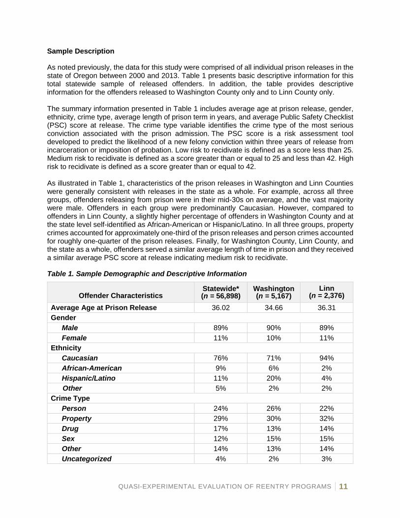
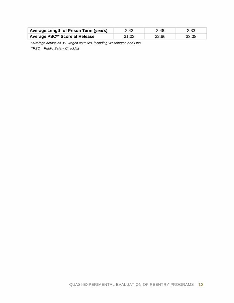
As noted previously, the data for this study were comprised of all individual prison releases in the state of Oregon between 2000 and 2013. Table 1 presents basic descriptive information for this total statewide sample of released offenders. In addition, the table provides descriptive information for the offenders released to Washington County only and to Linn County only. The summary information presented in Table 1 includes average age at prison release, gender, ethnicity, crime type, average length of prison term in years, and average Public Safety Checklist (PSC) score at release. The crime type variable identifies the crime type of the most serious conviction associated with the prison admission. The PSC score is a risk assessment tool developed to predict the likelihood of a new felony conviction within three years of release from incarceration or imposition of probation. Low risk to recidivate is defined as a score less than 25. Medium risk to recidivate is defined as a score greater than or equal to 25 and less than 42. High risk to recidivate is defined as a score greater than or equal to 42. As illustrated in Table 1, characteristics of the prison releases in Washington and Linn Counties were generally consistent with releases in the state as a whole. For example, across all three groups, offenders releasing from prison were in their mid-30s on average, and the vast majority were male. Offenders in each group were predominantly Caucasian. However, compared to offenders in Linn County, a slightly higher percentage of offenders in Washington County and at the state level self-identified as African-American or Hispanic/Latino. In all three groups, property crimes accounted for approximately one-third of the prison releases and person crimes accounted for roughly one-quarter of the prison releases. Finally, for Washington County, Linn County, and the state as a whole, offenders served a similar average length of time in prison and they received a similar average PSC score at release indicating medium risk to recidivate.
Table 1. Sample Demographic and Descriptive Information
Offender Characteristics Statewide* (n = 56,898)
Washington (n = 5,167)
Linn (n = 2,376)
Average Age at Prison Release 36.02 34.66 36.31 Gender
Male 89% 90% 89% Female 11% 10% 11%
Ethnicity Caucasian 76% 71% 94% African-American 9% 6% 2% Hispanic/Latino 11% 20% 4% Other 5% 2% 2%
Crime Type Person 24% 26% 22% Property 29% 30% 32% Drug 17% 13% 14% Sex 12% 15% 15% Other 14% 13% 14% Uncategorized 4% 2% 3%
QUASI-EXPERIMENTAL EVALUATION OF REENTRY PROGRAMS 12
Average Length of Prison Term (years) 2.43 2.48 2.33 Average PSC** Score at Release 31.02 32.66 33.08 *Average across all 36 Oregon counties, including Washington and Linn **PSC = Public Safety Checklist

QUASI-EXPERIMENTAL EVALUATION OF REENTRY PROGRAMS 13
Outcomes and Modeling Strategy
HB 3194 Section 45 (2013) (codified in ORS 423.557) provided a new statewide definition of recidivism. The definition includes the arrest, conviction, or incarceration for a new crime or for any reason within three years of prison release. SB 366 (2015) removed the language that includes recidivating events that occur for any reason.
This Reentry program evaluation focused on recidivating events for “new crimes” only; it did not include recidivating events that occurred for “any reason.” Recidivating events that occur for any reason include arrests or incarcerations for supervision revocations or sanctions.
To supply OSLC investigators with the relevant information for this analysis, the CJC combined arrest data from Oregon’s Law Enforcement Data System with conviction data from the Oregon Judicial Department and incarceration data from the Oregon Department of Corrections. Of note, a single offender could contribute to all three recidivism components, or a subset, depending on the criminal justice system’s response to the new criminal activity committed. As with past statewide recidivism analyses, this data did not include federal or out of state data. New criminal activity needed to be entered into electronic data systems to be captured as a recidivating event. If new criminal activity was informal, and was not entered into an electronic data system, then it was not captured as a recidivating event in this analysis.
Arrest Recidivism This data included arrests where the person was finger-printed. It did not include arrests where the person was not finger-printed or other types of law enforcement contact not resulting in arrest. Fingerprinting was required in arrests for all felony crimes, and for misdemeanor drug and sex crimes. Multiple arrests or multiple arrest charges were not accounted for. The analysis captured whether an offender was or was not arrested for a new crime within three years of release from incarceration or imposition of probation.
Conviction Recidivism This data included misdemeanor and felony convictions from Oregon’s 36 circuit courts. It did not include convictions from municipal courts or justice courts, as those courts were not part of the unified state court system. The analysis captured whether an offender was or was not convicted of a new crime (misdemeanor or felony) within three years of release from incarceration or imposition of probation.
Incarceration Recidivism Incarceration data included felony prison and felony jail sentences. The incarceration data included felony incarceration sentences only and did not include misdemeanor jail sentences or jail time served pre-trial. Oregon does not have a statewide data system that provides misdemeanor jail sentence information by conviction or county, and therefore misdemeanor incarceration data at the statewide level was not available. Multiple incarceration events were not accounted for. The analysis captured whether an offender was or was not incarcerated within three years of release from prison.
A detailed, technical explanation of the recidivism data structure and modeling formulation is provided in Appendix 1.
QUASI-EXPERIMENTAL EVALUATION OF REENTRY PROGRAMS 14
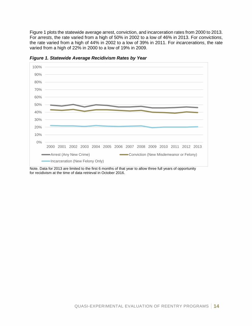
Figure 1 plots the statewide average arrest, conviction, and incarceration rates from 2000 to 2013. For arrests, the rate varied from a high of 50% in 2002 to a low of 46% in 2013. For convictions, the rate varied from a high of 44% in 2002 to a low of 39% in 2011. For incarcerations, the rate varied from a high of 22% in 2000 to a low of 19% in 2009.
Figure 1. Statewide Average Recidivism Rates by Year
Note. Data for 2013 are limited to the first 6 months of that year to allow three full years of opportunity for recidivism at the time of data retrieval in October 2016.
0%
10%
20%
30%
40%
50%
60%
70%
80%
90%
100%
2000 2001 2002 2003 2004 2005 2006 2007 2008 2009 2010 2011 2012 2013
Arrest (Any New Crime) Conviction (New Misdemeanor or Felony)
Incarceration (New Felony Only)
QUASI-EXPERIMENTAL EVALUATION OF REENTRY PROGRAMS 15
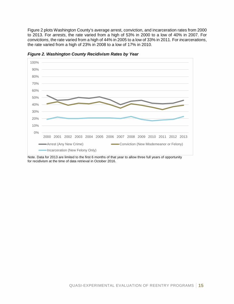
Figure 2 plots Washington County’s average arrest, conviction, and incarceration rates from 2000 to 2013. For arrests, the rate varied from a high of 53% in 2000 to a low of 40% in 2007. For convictions, the rate varied from a high of 44% in 2005 to a low of 33% in 2011. For incarcerations, the rate varied from a high of 23% in 2008 to a low of 17% in 2010.
Figure 2. Washington County Recidivism Rates by Year
Note. Data for 2013 are limited to the first 6 months of that year to allow three full years of opportunity for recidivism at the time of data retrieval in October 2016.
0%
10%
20%
30%
40%
50%
60%
70%
80%
90%
100%
2000 2001 2002 2003 2004 2005 2006 2007 2008 2009 2010 2011 2012 2013
Arrest (Any New Crime) Conviction (New Misdemeanor or Felony)
Incarceration (New Felony Only)
QUASI-EXPERIMENTAL EVALUATION OF REENTRY PROGRAMS 16
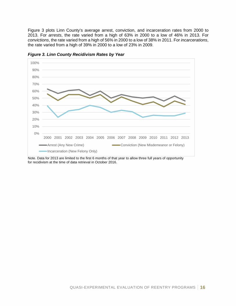
Figure 3 plots Linn County’s average arrest, conviction, and incarceration rates from 2000 to 2013. For arrests, the rate varied from a high of 63% in 2000 to a low of 46% in 2013. For convictions, the rate varied from a high of 56% in 2000 to a low of 38% in 2011. For incarcerations, the rate varied from a high of 39% in 2000 to a low of 23% in 2009.
Figure 3. Linn County Recidivism Rates by Year
Note. Data for 2013 are limited to the first 6 months of that year to allow three full years of opportunity for recidivism at the time of data retrieval in October 2016.
0%
10%
20%
30%
40%
50%
60%
70%
80%
90%
100%
2000 2001 2002 2003 2004 2005 2006 2007 2008 2009 2010 2011 2012 2013
Arrest (Any New Crime) Conviction (New Misdemeanor or Felony)
Incarceration (New Felony Only)

QUASI-EXPERIMENTAL EVALUATION OF REENTRY PROGRAMS 17
Findings
Evaluation Question 1: Across counties, did recidivism rates improve in the years following the start of Reentry programming?
The first question is broad—it focuses on the extent to which recidivism changed from year to year across all counties in the state. Because subsequent questions address changes for Washington and Linn specifically, this initial question was intended to determine whether, across all counties in the state, recidivism was decreasing during the years being evaluated. This provides important initial context for interpreting the results of the subsequent analyses. That is, if recidivism decreased significantly across all counties in the state during the years being evaluated, attributing improvements in Washington and Linn to Reentry programming would be challenging. The statistical model used to obtain recidivism estimates is detailed in Appendix 1.
Figure 4 illustrates the estimated rate of recidivism for arrests across all counties from 2000 to 2013. As described previously, the model included a coding strategy that served to average years 2000 to 2006, which was the “baseline period” before the start of Reentry programming. For the baseline period, the average rate of arrest recidivism was 46%. That is, of prison releases from 2000 to 2006, 46% were re-arrested within three years of release. Because this was an average for the seven years preceding Reentry programming, it provided a point of comparison for each year from 2007 to 2013. For arrests, there were no years from 2007 to 2013 when the estimated rate differed significantly from baseline. Generally, from 2007 to 2013, the rates of recidivism were consistent with the rates during the baseline period, from 2000 to 2006. The figure below displays the predicted probability for arrest recidivism by year; Appendix 3 provides each county’s actual recidivism rates for each year.
Figure 4. Predicted Probability of Arrest Recidivism Across Counties
Figure 5 illustrates the estimated rate of recidivism for convictions across all counties from 2000 to 2013. The baseline period is an average of the years before the start of Reentry programming,
0.30
0.40
0.50
0.60
2000-2006 2007 2008 2009 2010 2011 2012 2013
Prob
abilit
y

QUASI-EXPERIMENTAL EVALUATION OF REENTRY PROGRAMS 18
which was 40% for conviction recidivism. That is, of prison releases from 2000 to 2006, 40% were convicted for a new crime within three years of release. For convictions, the rates in 2010 (38%) and 2011 (37%) were significantly lower compared to the baseline period (see the large points marked on Figure 5). Generally, from 2007 to 2013, the rates of recidivism were consistent with the rates during the baseline period, from 2000 to 2006, and the years that were significantly different had lower rates of recidivism relative to the baseline period. The figure below displays the predicted probability for conviction recidivism by year; Appendix 3 provides each county’s actual recidivism rates for each year.
Figure 5. Predicted Probability of Conviction Recidivism Across Counties
Note. Large points on the line denote statistically significant differences relative to the baseline period.
0.30
0.40
0.50
2000-2006 2007 2008 2009 2010 2011 2012 2013
Prob
abilit
y
QUASI-EXPERIMENTAL EVALUATION OF REENTRY PROGRAMS 19
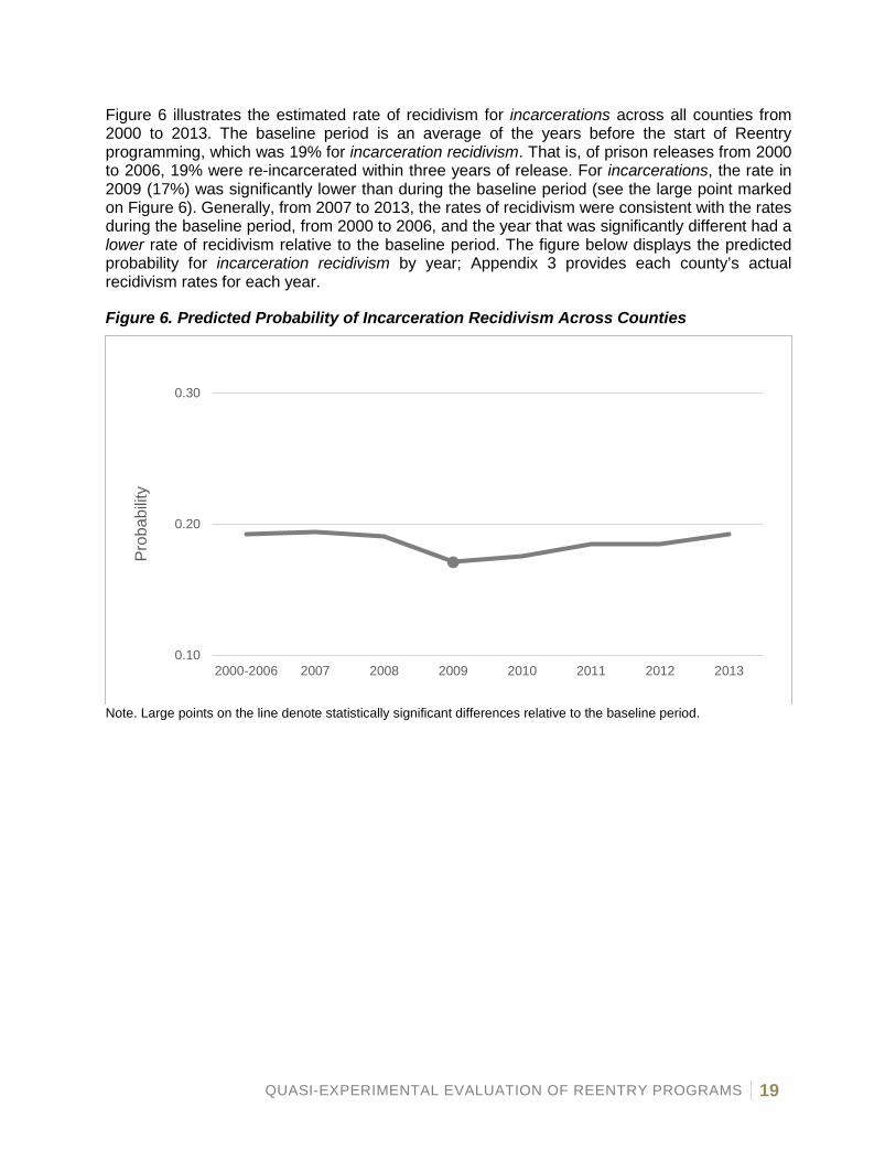
Figure 6 illustrates the estimated rate of recidivism for incarcerations across all counties from 2000 to 2013. The baseline period is an average of the years before the start of Reentry programming, which was 19% for incarceration recidivism. That is, of prison releases from 2000 to 2006, 19% were re-incarcerated within three years of release. For incarcerations, the rate in 2009 (17%) was significantly lower than during the baseline period (see the large point marked on Figure 6). Generally, from 2007 to 2013, the rates of recidivism were consistent with the rates during the baseline period, from 2000 to 2006, and the year that was significantly different had a lower rate of recidivism relative to the baseline period. The figure below displays the predicted probability for incarceration recidivism by year; Appendix 3 provides each county’s actual recidivism rates for each year.
Figure 6. Predicted Probability of Incarceration Recidivism Across Counties
Note. Large points on the line denote statistically significant differences relative to the baseline period.
0.10
0.20
0.30
2000-2006 2007 2008 2009 2010 2011 2012 2013
Prob
abilit
y
QUASI-EXPERIMENTAL EVALUATION OF REENTRY PROGRAMS 20
Evaluation Question 2: Across counties, were recidivism rates lower for those reporting greater use of pre-release Reach-Ins?
The association between a specific component of Reentry programming, pre-release Reach-Ins, and recidivism was evaluated. As with the preceding results, this question looks at the effect of Reach-Ins across all counties and does not specifically focus on Washington and Linn.
The data for evaluating this question were the same as described for Question 1, with the addition of the Reach-In rate variable. The rate of Reach-In use for each county was calculated from a statewide Reach-In Report. The Oregon Department of Corrections compiles this Reach-In Report every 6 months. For each county, the report tracks Reach-In contacts, including the individual offender, date of contact, type of contact, and individual conducting the Reach-In. The provided report included contacts from 2010 to 2017. However, for the present purposes, the report was limited to 2011, 2012, and 2013 because of limited use of the report in 2010 and to match the time-frame of the recidivism data. The data in the report were limited to (a) contacts occurring prior to prison release and (b) cases where the contact could be linked to a specific prison release (of note, supplementary models also limited the contacts to those that occurred in-person, and the results were highly consistent). For each county, the result was a single, average score from 2011 to 2013 that reflected the proportion of prison releases receiving a Reach-In prior to release. This single, county-level score was entered as a predictor in the model detailed for Question 1, testing the direction and magnitude of the association between county-reported Reach-In use and recidivism.
QUASI-EXPERIMENTAL EVALUATION OF REENTRY PROGRAMS 21
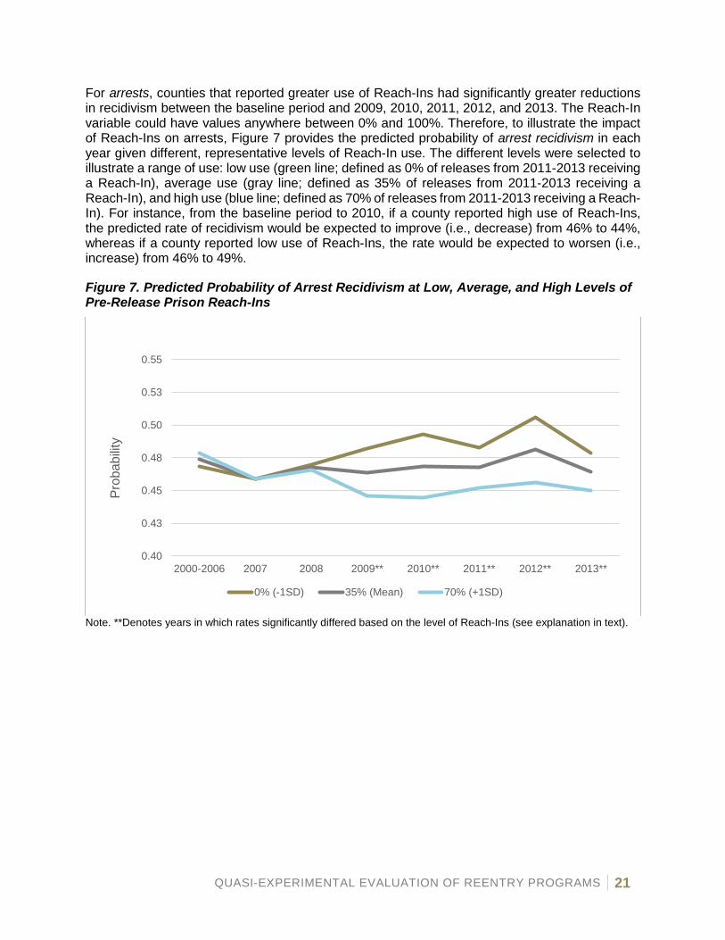
For arrests, counties that reported greater use of Reach-Ins had significantly greater reductions in recidivism between the baseline period and 2009, 2010, 2011, 2012, and 2013. The Reach-In variable could have values anywhere between 0% and 100%. Therefore, to illustrate the impact of Reach-Ins on arrests, Figure 7 provides the predicted probability of arrest recidivism in each year given different, representative levels of Reach-In use. The different levels were selected to illustrate a range of use: low use (green line; defined as 0% of releases from 2011-2013 receiving a Reach-In), average use (gray line; defined as 35% of releases from 2011-2013 receiving a Reach-In), and high use (blue line; defined as 70% of releases from 2011-2013 receiving a Reach-In). For instance, from the baseline period to 2010, if a county reported high use of Reach-Ins, the predicted rate of recidivism would be expected to improve (i.e., decrease) from 46% to 44%, whereas if a county reported low use of Reach-Ins, the rate would be expected to worsen (i.e., increase) from 46% to 49%.
Figure 7. Predicted Probability of Arrest Recidivism at Low, Average, and High Levels of Pre-Release Prison Reach-Ins
Note. **Denotes years in which rates significantly differed based on the level of Reach-Ins (see explanation in text).
0.40
0.43
0.45
0.48
0.50
0.53
0.55
2000-2006 2007 2008 2009** 2010** 2011** 2012** 2013**
Prob
abilit
y
0% (-1SD) 35% (Mean) 70% (+1SD)

QUASI-EXPERIMENTAL EVALUATION OF REENTRY PROGRAMS 22
For convictions, Figure 8 illustrates the predicted probability of recidivism in each year based on different levels of Reach-In use: low use (green line; 0% of releases from 2011-2013 receiving a Reach-In), average use (gray line; 35% of releases from 2011-2013 receiving a Reach-In), and high use (blue line; 70% of releases from 2011-2013 receiving a Reach-In). In years 2009 and 2010, higher levels of Reach-In use were associated with greater reductions relative to the baseline period. For example, if a county reported high use of Reach-Ins, in the baseline period, the predicted conviction rate would be 40%, and in 2010, this would be expected to decrease to 38%. In contrast, if a county reported low use of Reach-Ins, the 40% baseline rate of convictions would be expected to decrease to 39% in 2010.
Figure 8. Predicted Probability of Conviction Recidivism at Low, Average, and High Levels of Pre-Release Prison Reach-Ins
Note. **Denotes years in which rates significantly differed based on the level of Reach-Ins (see explanation in text).
0.30
0.33
0.35
0.38
0.40
0.43
0.45
2000-2006 2007 2008 2009** 2010** 2011 2012 2013
Prob
abilit
y
0% (-1SD) 35% (Mean) 70% (+1SD)
QUASI-EXPERIMENTAL EVALUATION OF REENTRY PROGRAMS 23
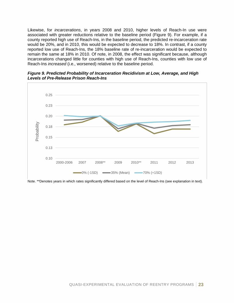
Likewise, for incarcerations, in years 2008 and 2010, higher levels of Reach-In use were associated with greater reductions relative to the baseline period (Figure 9). For example, if a county reported high use of Reach-Ins, in the baseline period, the predicted re-incarceration rate would be 20%, and in 2010, this would be expected to decrease to 18%. In contrast, if a county reported low use of Reach-Ins, the 18% baseline rate of re-incarceration would be expected to remain the same at 18% in 2010. Of note, in 2008, the effect was significant because, although incarcerations changed little for counties with high use of Reach-Ins, counties with low use of Reach-Ins increased (i.e., worsened) relative to the baseline period.
Figure 9. Predicted Probability of Incarceration Recidivism at Low, Average, and High Levels of Pre-Release Prison Reach-Ins
Note. **Denotes years in which rates significantly differed based on the level of Reach-Ins (see explanation in text).
0.10
0.13
0.15
0.18
0.20
0.23
0.25
2000-2006 2007 2008** 2009 2010** 2011 2012 2013
Prob
abilit
y
0% (-1SD) 35% (Mean) 70% (+1SD)
QUASI-EXPERIMENTAL EVALUATION OF REENTRY PROGRAMS 24
Evaluation Question 3: Did Washington and Linn Counties improve more than other counties after Reentry programming?
The prior questions apply across all counties in the state; Question 3, however, focuses on Washington and Linn. In this model, all counties receive an estimate that describes their change between the baseline period and the given year (from 2007 to 2013). This estimate, called a “rate multiplier,” reflects the county’s change as a proportion of the statewide change for the same year. More specifically, a value of 1.0 indicates that the change for a particular county was the same as the average change across the state. Values above 1.0 indicate greater increases relative to the statewide rate (for example, 1.2 reflects a 20% increase), and values less than 1.0 indicate greater decreases relative to the statewide rate (for example, 0.8 reflects a 20% decrease).

QUASI-EXPERIMENTAL EVALUATION OF REENTRY PROGRAMS 25
Figure 10 was generated to provide an example of how each county provides a separate line in the graph; Figure 10 is for arrest recidivism. There is a line for each county, beginning in 2007 and ending in 2013, and the location of the line reflects the county’s rate multiplier over time. As such, a lower position on the graph indicates that, relative to the average change across all counties, a county had greater reductions in recidivism. These figures are essential to evaluating Reentry programming efforts in Washington and Linn Counties. The strength is that they compare each county to its own prior performance, and because all counties are modeled—including those utilizing fewer, or no, Reentry programming components—if Washington and Linn exhibit greater improvements relative to the statewide average, there is evidence of a Reentry programming effect.
It is important to emphasize that the graphs do not illustrate the actual rates of recidivism. Rather, they illustrate the change in recidivism. Because of this, for any location on the graph, a county’s actual rate of recidivism could be high or low, but for this evaluation, improvement in recidivism (that is, a lower position on the graph) is the focus. Supplementary information about statewide rank in actual recidivism rates is presented in Evaluation Question 4, and the descriptive rates for each year for each county are provided in Appendix 3.
Figure 10. Each County’s Annual Rate Multiplier for Arrest Recidivism (Each County’s Annual Change from Baseline Compared to the Statewide Change from Baseline)
0.40
0.60
0.80
1.00
1.20
1.40
1.60
2007 2008 2009 2010 2011 2012 2013
Rat
e M
ultip
lier

QUASI-EXPERIMENTAL EVALUATION OF REENTRY PROGRAMS 26
Figure 11 emphasizes Washington and Linn Counties by changing all the other county lines shown in Figure 10 to gray. For arrest recidivism (Figure 11), the statewide average change, at the position of 1.00 by definition, is highlighted by the broken line across all years. There was considerable variability in improvement from year to year and from county to county. The figure illustrates that, in each year following the start of Reentry programming, both Washington and Linn Counties, compared to their own baseline periods, had greater reductions in arrest recidivism than did the state as a whole (that is, their lines are located below the broken, average line), and their reductions are greater than nearly all other individual counties in the state. The large points on Washington and Linn’s lines indicate the years when they had significantly greater reductions in arrests relative to the statewide average. For these analyses, statistical significance means that the estimated rate multiplier is precise enough that there is a very low likelihood of it crossing 1.00—that is, there is a high degree of confidence that the year reflects true improvement. Linn improved significantly more relative to the statewide average in 2009 and 2013, and for Washington, improvements were significant in 2007, 2011, and 2012.
Figure 11. Each County’s Annual Rate Multiplier for Arrest Recidivism (Each County’s Annual Change from Baseline Compared to the Statewide Change from Baseline), Washington and Linn Counties Identified
Note. Large points on the line denote statistically significant differences relative to the statewide average.
0.40
0.60
0.80
1.00
1.20
1.40
1.60
2007 2008 2009 2010 2011 2012 2013
Rat
e M
ultip
lier
Linn
Washington
QUASI-EXPERIMENTAL EVALUATION OF REENTRY PROGRAMS 27
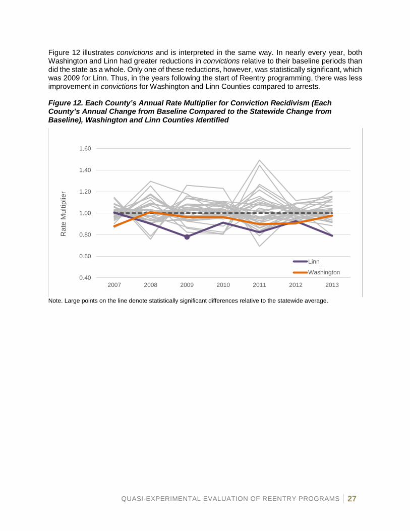
Figure 12 illustrates convictions and is interpreted in the same way. In nearly every year, both Washington and Linn had greater reductions in convictions relative to their baseline periods than did the state as a whole. Only one of these reductions, however, was statistically significant, which was 2009 for Linn. Thus, in the years following the start of Reentry programming, there was less improvement in convictions for Washington and Linn Counties compared to arrests.
Figure 12. Each County’s Annual Rate Multiplier for Conviction Recidivism (Each County’s Annual Change from Baseline Compared to the Statewide Change from Baseline), Washington and Linn Counties Identified
Note. Large points on the line denote statistically significant differences relative to the statewide average.
0.40
0.60
0.80
1.00
1.20
1.40
1.60
2007 2008 2009 2010 2011 2012 2013
Rat
e M
ultip
lier
Linn
Washington
QUASI-EXPERIMENTAL EVALUATION OF REENTRY PROGRAMS 28
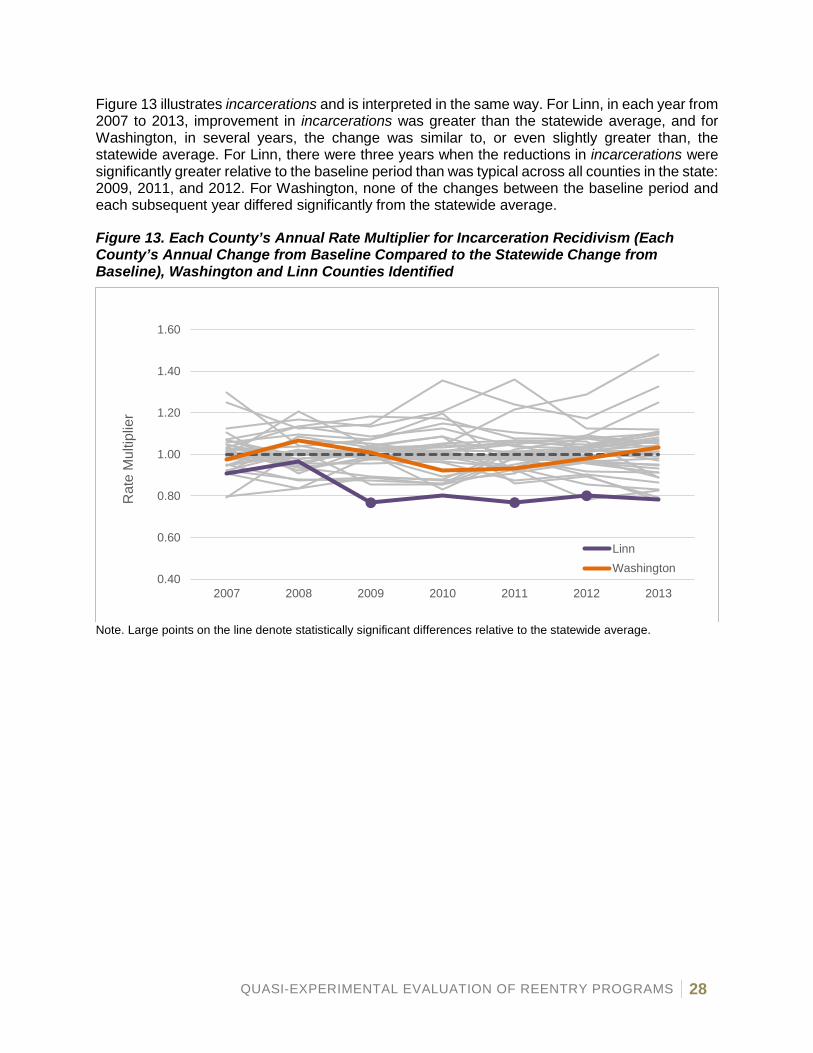
Figure 13 illustrates incarcerations and is interpreted in the same way. For Linn, in each year from 2007 to 2013, improvement in incarcerations was greater than the statewide average, and for Washington, in several years, the change was similar to, or even slightly greater than, the statewide average. For Linn, there were three years when the reductions in incarcerations were significantly greater relative to the baseline period than was typical across all counties in the state: 2009, 2011, and 2012. For Washington, none of the changes between the baseline period and each subsequent year differed significantly from the statewide average.
Figure 13. Each County’s Annual Rate Multiplier for Incarceration Recidivism (Each County’s Annual Change from Baseline Compared to the Statewide Change from Baseline), Washington and Linn Counties Identified
Note. Large points on the line denote statistically significant differences relative to the statewide average.
0.40
0.60
0.80
1.00
1.20
1.40
1.60
2007 2008 2009 2010 2011 2012 2013
Rat
e M
ultip
lier
LinnWashington

QUASI-EXPERIMENTAL EVALUATION OF REENTRY PROGRAMS 29
Figure 14 illustrates the results of a simplified version of the models just reported. Instead of comparing each individual year from 2007 to 2013 to the baseline period, this model compares the average across 2007 to 2013 to the baseline period. This yields a single “rate multiplier” for each county, and as such, each county is represented by a single dot on the graph. As with the prior graphs, the statewide average improvement relative to the baseline period is represented by the broken line at 1.0. Additionally, because each county has a single rate multiplier, the counties are ordered by their degree of improvement relative to the statewide average. The figure illustrates that Washington and Linn Counties had two of the top three rates of improvement in arrest recidivism in the state for the period following the start of Reentry programming relative to the baseline period. Further, for the two counties, these rates were statistically significant.
Figure 14. Each County’s Intervention Period (2007-2013) Rate Multiplier for Arrest Recidivism (Each County’s Change from Baseline to Intervention Period Compared to the Statewide Change), Washington and Linn Counties Identified
Note. Purple = Linn; Orange = Washington; Points with a solid color denote statistically significant improvement.
0.4
0.6
0.8
1
1.2
1.4
1.6
Rat
e M
ultip
lier
Counties (Most to Least Improved)
QUASI-EXPERIMENTAL EVALUATION OF REENTRY PROGRAMS 30
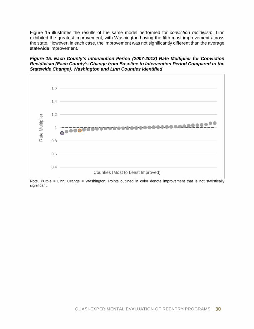
Figure 15 illustrates the results of the same model performed for conviction recidivism. Linn exhibited the greatest improvement, with Washington having the fifth most improvement across the state. However, in each case, the improvement was not significantly different than the average statewide improvement.
Figure 15. Each County’s Intervention Period (2007-2013) Rate Multiplier for Conviction Recidivism (Each County’s Change from Baseline to Intervention Period Compared to the Statewide Change), Washington and Linn Counties Identified
Note. Purple = Linn; Orange = Washington; Points outlined in color denote improvement that is not statistically significant.
0.4
0.6
0.8
1
1.2
1.4
1.6
Rat
e M
ultip
lier
Counties (Most to Least Improved)
QUASI-EXPERIMENTAL EVALUATION OF REENTRY PROGRAMS 31
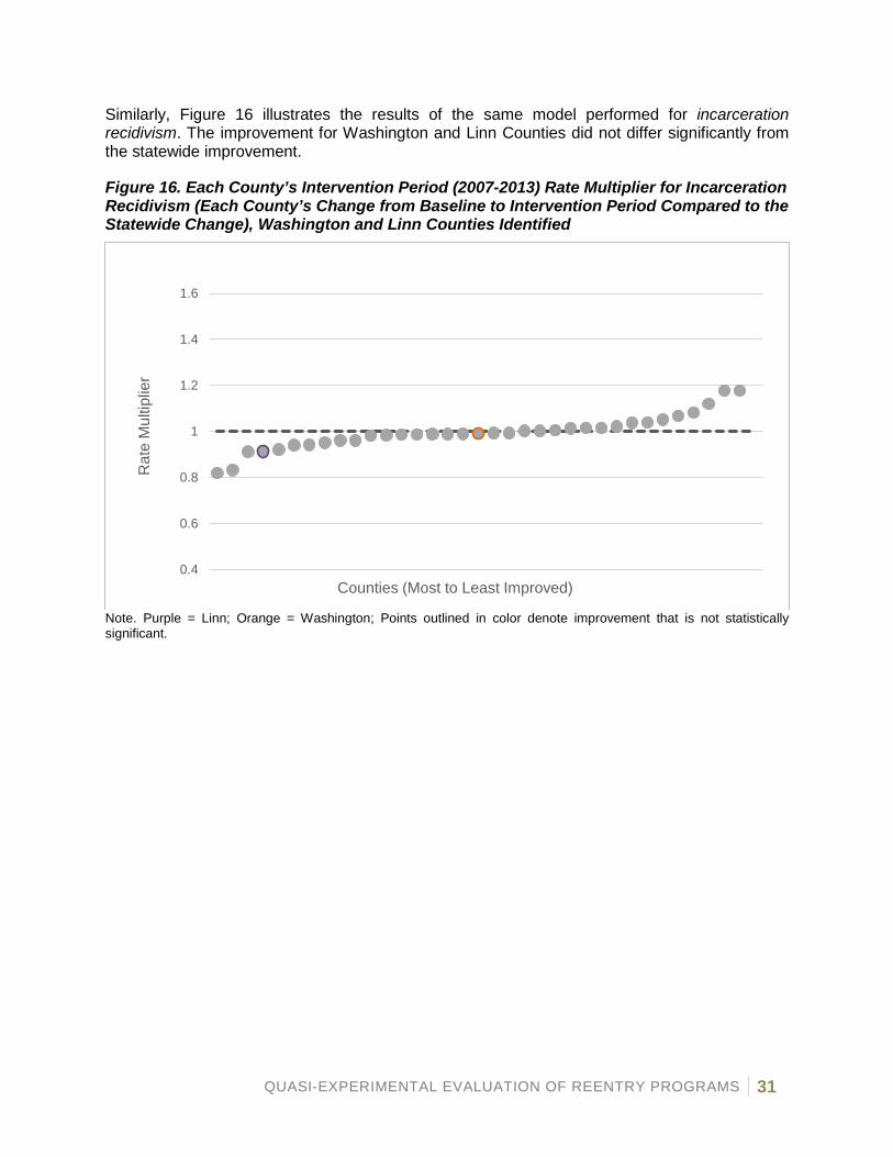
Similarly, Figure 16 illustrates the results of the same model performed for incarceration recidivism. The improvement for Washington and Linn Counties did not differ significantly from the statewide improvement.
Figure 16. Each County’s Intervention Period (2007-2013) Rate Multiplier for Incarceration Recidivism (Each County’s Change from Baseline to Intervention Period Compared to the Statewide Change), Washington and Linn Counties Identified
Note. Purple = Linn; Orange = Washington; Points outlined in color denote improvement that is not statistically significant.
0.4
0.6
0.8
1
1.2
1.4
1.6
Rat
e M
ultip
lier
Counties (Most to Least Improved)

QUASI-EXPERIMENTAL EVALUATION OF REENTRY PROGRAMS 32
Evaluation Question 4: For Washington and Linn Counties, did recidivism rates improve relative to other counties in the state?
The prior questions focus on Washington and Linn’s change in recidivism, results that, for this evaluation, are the primary indicators of Reentry programming’s effect on recidivism. However, because the results focus on change, they do not explicitly describe the overall levels of recidivism. For instance, it could be possible for a county to exhibit no improvement in arrest recidivism from the baseline period to the years following the start of Reentry programming, but across all years, that county could have the lowest arrest recidivism rate in the state. Likewise, a county could exhibit great improvement in recidivism but still have a rate much higher than other counties in the state. This was not seen as critical information for determining whether there was a Reentry programming effect because such an effect is, by definition, focused on change. However, for interpreting such effects, the actual recidivism rates provided important context. As such, additional, descriptive figures were created to illustrate each county’s rank in the state during the baseline period and during the years following the start of Reentry programming.
Figure 17 illustrates the state rank on arrest recidivism rates for each county, with a different colored line for each county.
Figure 17. All Counties Rank Ordered by Arrest Recidivism Before (2000-2006) and After (2007-2013) Start of Reentry Programming
02468
1012141618202224262830323436
2000-2006 2007-2013
Ran
k
QUASI-EXPERIMENTAL EVALUATION OF REENTRY PROGRAMS 33
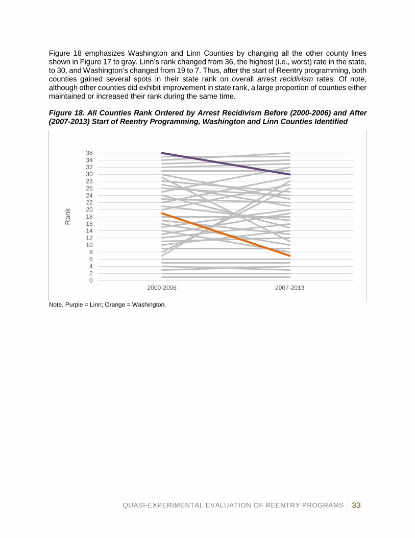
Figure 18 emphasizes Washington and Linn Counties by changing all the other county lines shown in Figure 17 to gray. Linn’s rank changed from 36, the highest (i.e., worst) rate in the state, to 30, and Washington’s changed from 19 to 7. Thus, after the start of Reentry programming, both counties gained several spots in their state rank on overall arrest recidivism rates. Of note, although other counties did exhibit improvement in state rank, a large proportion of counties either maintained or increased their rank during the same time.
Figure 18. All Counties Rank Ordered by Arrest Recidivism Before (2000-2006) and After (2007-2013) Start of Reentry Programming, Washington and Linn Counties Identified
Note. Purple = Linn; Orange = Washington.
02468
1012141618202224262830323436
2000-2006 2007-2013
Ran
k
QUASI-EXPERIMENTAL EVALUATION OF REENTRY PROGRAMS 34
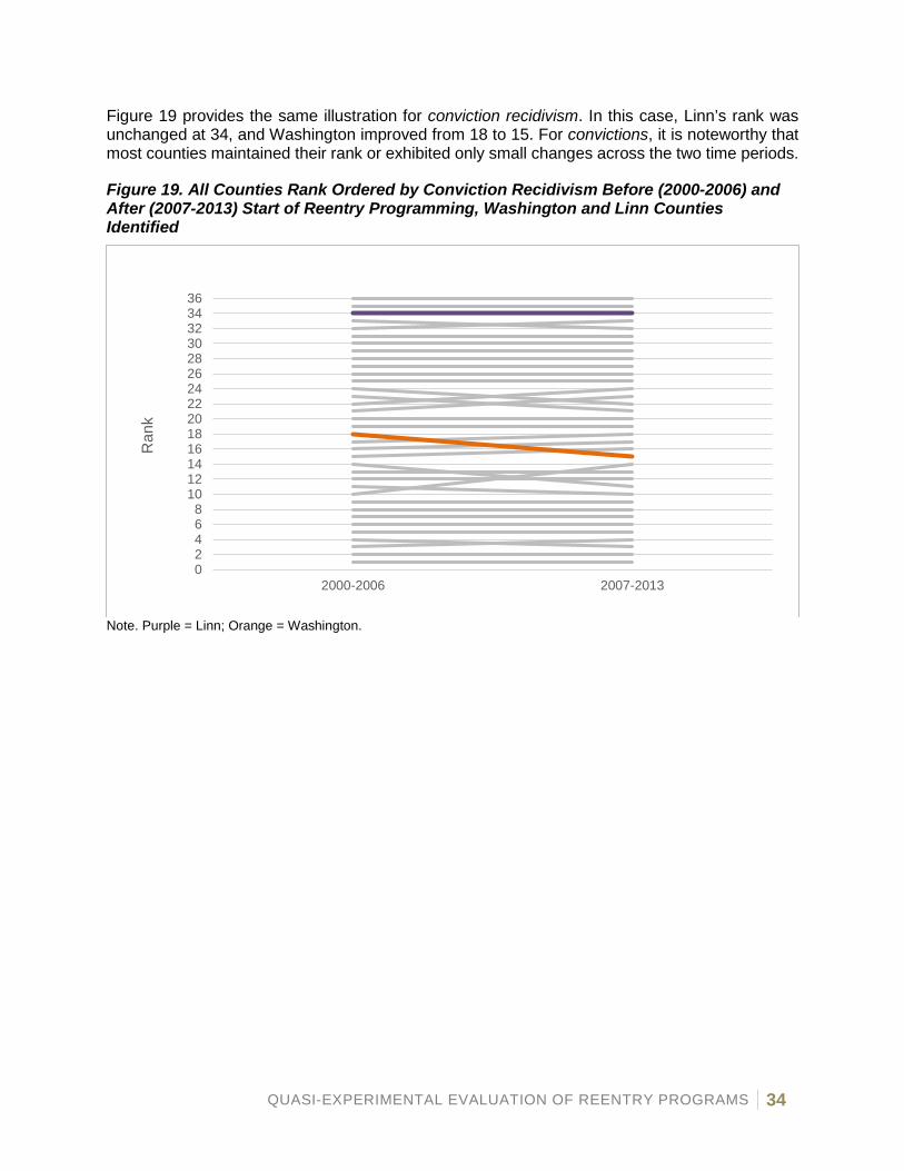
Figure 19 provides the same illustration for conviction recidivism. In this case, Linn’s rank was unchanged at 34, and Washington improved from 18 to 15. For convictions, it is noteworthy that most counties maintained their rank or exhibited only small changes across the two time periods.
Figure 19. All Counties Rank Ordered by Conviction Recidivism Before (2000-2006) and After (2007-2013) Start of Reentry Programming, Washington and Linn Counties Identified
Note. Purple = Linn; Orange = Washington.
02468
1012141618202224262830323436
2000-2006 2007-2013
Ran
k
QUASI-EXPERIMENTAL EVALUATION OF REENTRY PROGRAMS 35
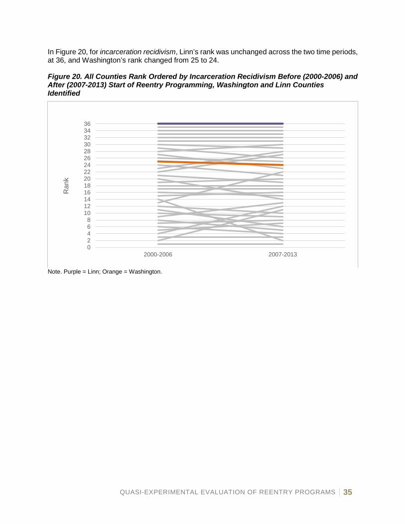
In Figure 20, for incarceration recidivism, Linn’s rank was unchanged across the two time periods, at 36, and Washington’s rank changed from 25 to 24.
Figure 20. All Counties Rank Ordered by Incarceration Recidivism Before (2000-2006) and After (2007-2013) Start of Reentry Programming, Washington and Linn Counties Identified
Note. Purple = Linn; Orange = Washington.
02468
1012141618202224262830323436
2000-2006 2007-2013
Ran
k

QUASI-EXPERIMENTAL EVALUATION OF REENTRY PROGRAMS 36
Reentry Program Effect Size: Preliminary Estimate Based on Reach-In Data
The state requested a summary for the magnitude of Reentry programming’s effect, focused specifically on arrest recidivism. Effect sizes and odds ratios (OR) are the primary ways of quantifying, in standardized (i.e., interpretable) units, the overall magnitude of a particular intervention’s effect. However, the quality of these estimates depends on the study design. Data from RCTs are ideally suited to quantifying the magnitude of an intervention’s effect. For the present quasi-experimental evaluation, the limited data on each county’s use of Reentry programming, aside from Washington and Linn Counties, made the data less well-suited to estimating the overall magnitude of Reentry programming. However, Evaluation Question 2 included data about each county’s use of Reach-Ins, making it possible to glean some information about the magnitude of an effect in the present quasi-experimental evaluation. More specifically, Evaluation Question 2 was selected for two reasons: (1) Reach-Ins are a hallmark component of Reentry programs; and (2) data pertaining to the use of Reach-Ins were available for every county in the state. In contrast, the other Evaluation Questions focused on the performance of Washington and Linn Counties specifically, and although their change is compared to change across the state, the models do not include information about other counties’ use of Reentry programming. For the present question, given how the models performed, the magnitude of the Reach-In effect can be summarized as OR. For example, if there are two groups, the OR reflects the odds of the event in one group relative to the odds of the event in the other group. An OR of 1.00 means that the odds are the same in both groups. An OR greater than 1.00 means that the odds are higher in the focal group, and an OR less than 1.00 means that the odds are lower in the focal group. Thus, for the present evaluation, an OR less than 1.00 is desirable, indicating that arrest recidivism was less likely to occur given greater use of Reach-Ins. To summarize the magnitude of the overall Reach-In effect, the model estimates were used to compute OR. Depending on the focus, a wide range of OR could be computed. In this case, the computed OR reflect the effect of Reach-Ins on the average change in arrest recidivism across years 2010-2012 relative to years 2000-2006 (of note, 2013 was excluded because data were only available for the first half of the year, and years 2007-2009 were excluded because they preceded the years covered by the Reach-In Report). As in Figure 7, the OR were computed both for high and average levels of Reach-In use relative to no Reach-In use.
• For 0% Reach-Ins, the average probability of arrest recidivism increased from 47% in 2000-2006 to 49% in 2010-2012. This corresponds to OR = 1.11.
• For 35% (i.e., average) Reach-Ins, the average probability of arrest recidivism was constant at 47% in 2000-2006 and 47% in 2010-2012. This corresponds to OR = 1.00.
• For 70% (i.e., high) Reach-Ins, the average probability of arrest recidivism decreased from 48% in 2000-2006 to 45% in 2010-2012. This corresponds to OR = 0.89.
• The effect of high and average Reach-In use relative to no Reach-In use was OR = 0.80 (i.e., 0.89 / 1.11) and OR = 0.90 (i.e., 1.00 / 1.11), respectively.
In sum, this indicates that the change in odds of arrest recidivism associated with high and average use of Reach-Ins was 80% and 90% of the change associated with no use of Reach-Ins, respectively. Stated differently, the odds of arrest recidivism associated with high and average use of Reach-Ins was 20% and 10% lower than the odds associated with no use of Reach-Ins, respectively.

QUASI-EXPERIMENTAL EVALUATION OF REENTRY PROGRAMS 37
Conclusion and Recommendations
This report describes the results of a quasi-experimental evaluation of Reentry programs in Washington and Linn Counties. Overall, results provide evidence from multiple sources indicating the Reentry programs as delivered in Washington and Linn Counties are associated with reduced recidivism among offenders. Compared to statewide trends, Linn County had years with greater reductions in recidivism for arrests, convictions, and prison use. Compared to statewide trends, Washington County had years with greater reductions in recidivism for arrests and convictions, and kept pace with the statewide change in prison use. Such findings are consistent with a large-scale meta-analysis indicating that Reentry programs are effective at reducing criminal recidivism.4 This is particularly true for Reentry programs that are initiated when offenders are still incarcerated (i.e., a Reach-in) and continue through their release to the community, as is the case for the programs in Washington and Linn. As an example, when there was a high rate of pre-release Reach-ins, arrest recidivism was up to 20% lower than when there was no use of Reach-Ins.
An important caveat is that evidence for a Reentry programming effect was not universal and was most consistently observed on arrests versus convictions or incarcerations. The reasons for this discrepancy are not entirely clear from the present evaluation. However, it could be argued that Reentry programming, which aims to directly support offenders, should have a greater impact on arrests because this is the indicator most closely linked to offender behavior. Convictions and incarcerations, on the other hand, are likely more impacted by county-level forces not specifically targeted by Reentry programs (e.g., resources and practices of the local District Attorney’s Office).
The present evaluation also was limited to existing data and a quasi-experimental design. Given these programs have multiple components, future research should identify the components that generate the greatest reductions in recidivism. Studies should also attempt to standardize program elements and monitor implementation fidelity to ensure all elements are delivered as intended. Lastly, although the current context did not permit evaluation of Reentry programs in an RCT, such a design would provide a more rigorous test of Reentry program efficacy and overcome limitations related to a quasi-experimental design.
Although further evaluation (as suggested above) could provide definitive proof, the conclusion of this evaluation is that Reentry programs as currently delivered in Washington and Linn Counties have been a success and there is quasi-experimental support for continued funding of these programs.
4 Ndrecka, M. (2014). The impact of reentry programs on recidivism: A meta-analysis (Unpublished doctoral dissertation). University of Cincinnati, Ohio.
QUASI-EXPERIMENTAL EVALUATION OF REENTRY PROGRAMS 38
Appendix 1: Technical Explanation of Evaluation Design and Statistical Analyses
This appendix provides a technical description of the evaluation design and data analysis strategy for the Reentry programming evaluation. The section begins with a general description of the evaluation design and statistical method. This is followed by a description of the data and modeling features across the four evaluation questions. When evaluating interventions, one of the main goals is to be able to attribute observed effects to the intervention being investigated rather than other potentially influential factors. To achieve this goal, the strongest approach tends to be an RCT. However, the rigor afforded by an RCT design comes with a steep time and resource cost—the RCT is not feasible in many real-world evaluation settings. Because of this, alternative quasi-experimental designs must be considered and, along with such designs, the use of advanced statistical methods. The combination of quasi-experimental designs and sophisticated statistical methodologies makes it possible to provide compelling evidence to support, or reject, the intervention being investigated. For the present evaluation, there were numerous challenges to be addressed: For the intervention itself, there were different versions of Reentry programming efforts. That is, Reentry programming was not a standard package, implemented in the same way in each county. Likewise, two counties were the specific focus of this evaluation, yet across the state, multiple counties reported using various aspects of Reentry programming. For any of these counties, the scope and intensity of Reentry programming efforts could have evolved and fluctuated over time. Related to this, much information that would be useful for an evaluation (for example, related to the type, intensity, and timing of Reentry programming efforts) was not—understandably—tracked systematically for evaluation purposes. Finally, in counties that utilized Reentry programming, every prison release did not necessarily receive the intervention or all aspects of the program. Tracking of the Reentry programming delivery to individual offenders did not begin until later, and this varied from county to county. Combined, these factors illustrate the types of challenges—which are all common in such investigations—that had to be addressed by the quasi-experimental evaluation. The overarching goal was to evaluate the impact of Reentry programming in Washington and Linn Counties, which raises the question: In a non-randomized design, how is it possible to determine whether Reentry programming has had an effect? In these counties, Reentry programming efforts began in 2007. There were two initial options for an evaluation design. With multiple years of data available, one option would be to test whether, for these counties, the recidivism rates decreased beginning in 2007. However, if there were decreases, there is no way to know if they are attributable to other factors. Perhaps counties not using Reentry programming decreased during the same time. A second option could be to identify suitable comparison counties. There are statistical procedures for this, known as propensity score matching. However, the procedures require data (and levels of data) that were not available across the state and are associated with a series of other stringent assumptions; essentially, the results of the propensity score matching procedures are only as good as the data being used to match offenders accurately, and such data do not exist at present for Oregon counties. Thus, propensity score matching was not suitable for answering the questions in this evaluation. Despite the challenges, however, there were a few factors that considerably strengthened the evaluation. Recidivism data were available for each county in the state, and the data spanned a wide range of years. Because the available data preceded the start of Reentry programming, there was a “baseline period” where each county’s recidivism could serve as a comparison for its
QUASI-EXPERIMENTAL EVALUATION OF REENTRY PROGRAMS 39
recidivism after the start of Reentry programming. This had two key benefits: First, each county could serve as its own comparison group (that is, comparing recidivism before and after the start of Reentry programming). Second, the changes occurring in Washington and Linn Counties could be compared to the changes occurring in the state as a whole during the same time. Combined, these features addressed concerns about suitable control groups and also about changes that would have naturally occurred, even in the absence of Reentry programming. Further, the recidivism data were obtained from a standardized data source and directly comparable from county to county. Additionally, sophisticated statistical models were available for flexibly and simultaneously obtaining the comparisons just described. Finally, in the evaluation literature, such methods had been developed, implemented, and carefully described, including an evaluation (see below) that shared many of the features just described. As detailed by Gibbons and colleagues,5 in the Illinois child welfare system, two counties were identified that had disproportionately high rates of removing African American children from their homes. To address this, a county-level investigation was conducted, and from the findings, an intervention was developed and implemented in the two counties. Gibbons and colleagues were tasked with evaluating retrospectively the impact of the intervention. The outcome was county-level foster care placement rates across two years, the year before and the year after the intervention, and the analysis utilized data from all counties in the state. The statistical analyses were based on an approach that accommodated each county having data before and after the intervention and was tailored to the outcome being a rate (that is, the number of placements adjusted for the county population size). The model included a term to estimate, across counties, the average change from the year preceding the intervention to the year following the intervention. However, the results also included a term for each county that quantifies how it differed from the statewide average change. This term, labeled a “rate multiplier,” had a straightforward interpretation for each county: A value of 1.0 meant that the county’s change from before to after the intervention was the same as the average change across the state. A value less than 1.0 meant that the county had a larger decrease than was typical across the state (for example, 0.8 would mean that the county’s rate decreased by 20% more than the average change across the state). Likewise, a value greater than 1.0 meant that the county had a larger increase than was typical across the state (for example, 1.2 would mean that the county’s rate increased by 20% more than the average change across the state). This provided an efficient, highly informative method for evaluating the performance of an individual county. Further, the results were based on how much, and in what direction, a county changes relative to its prior performance, and this change is then compared to how, as a whole, counties across the state changed during the same period of time. To test whether the individual county rate multipliers were statistically significant, Gibbons and colleagues used additional estimates from the model to calculate “confidence intervals” around the estimate. Rate multipliers with a very high probability of not exceeding 1.0 were considered statistically significant; in other words, the investigators were confident the
5 Gibbons, R. D., Hur, K., Bhaumik, D. K., & Bell, C. C. (2007). Profiling of county-level foster care placements using random-effects Poisson regression models. Health Services and Outcomes Research Methodology, 7, 97-108. For related methods, also see: Gibbons, R. D., Segawa, E., Karbatsos, G., Amatya, A. K., Bhaumik, D. K., Brown, C. H., Kapur, K. et al. (2008). Mixed-effects Poisson regression analysis of adverse event reports: The relationship between antidepressants and suicide. Statistics in Medicine, 27, 1814-1833. Gibbons, R. D., Hur, K., Bhaumik, D. K., & Mann, J. (2005). The relationship between antidepressant medication use and rate of suicide. Archives of General Psychiatry, 62, 165-172.
QUASI-EXPERIMENTAL EVALUATION OF REENTRY PROGRAMS 40
county improved relative to the statewide average. The statistical and technical description of these procedures, as applied to the present evaluation, is provided below. The Reentry programming evaluation had three key differences from Gibbons et al. First, in their evaluation, two counties received the experimental intervention—the other counties in the state did not receive any aspects of the intervention. In contrast, for this evaluation, other counties in Oregon may have implemented aspects of Reentry programming. Second, in their evaluation, the two counties received identical versions of the intervention; whereas in the Reentry evaluation, Washington and Linn Counties likely implemented slightly different versions of Reentry programming. Third, their evaluation was based on data from two years; whereas the Reentry evaluation could utilize data from 2000 to 2013. The first two were potential limitations of this evaluation; the third, however, was a strength and is described next. Gibbons and colleagues’ approach was straightforwardly applied to the Reentry programming evaluation data. There were three main differences. First, the model was extended to accommodate fourteen, rather than two, years of data. This was implemented in a single, simultaneous model, and the interpretation for any given year directly mirrors that for Gibbons and colleagues. Second, the placement rate data for Gibbons and colleagues were, by definition, county-level rates. For the Reentry programming evaluation, however, offender-level recidivism data were available for each year within each county. This improved accuracy for interpretation of results, but required inclusion of an additional term in the model; however, the impact on the estimates and interpretation is unchanged. Finally, for Gibbons and colleagues, the comparison year was the single year prior to the implementation of the intervention. For the Reentry programming, the comparison was defined to be years 2000 to 2006; that is, the seven years prior to the start of Reentry programming were modeled so that they formed an average recidivism rate for each county. In this report, this range of years preceding Reentry programming is referred to as the “baseline period.” One final note is that for this evaluation, reference to specific years reflects the year of release from prison. For example, the recidivism rate from 2013 reflects the percentage of prison releases in 2013 that were arrested, convicted, or incarcerated within three years of the specific release date in 2013. Supplementary models were performed that compared the average recidivism from 2007 to 2013 (rather than year-by-year) to the average recidivism during the baseline period (2000 to 2006). The application of Gibbons and colleagues’ method to this evaluation provided the primary test of Reentry programming’s impact. However, additional sources of evidence were considered to improve confidence in the conclusions; this is common when investigations are limited to a quasi-experimental evaluation. As such, the findings are reported as answers to a series of evaluation questions, each of which was considered one aspect of evaluating Reentry programming. Together, these evaluation questions form the sources of evidence to inform a conclusion about the impact of Reentry programs. The specific four questions were:
Evaluation Question 1: Across counties, did recidivism rates improve in the years following the start of Reentry programming?
Evaluation Question 2: Across counties, were recidivism rates lower for those reporting greater use of pre-release Reach-Ins?
Evaluation Question 3: Did Washington and Linn Counties improve more than other counties after Reentry programming?
QUASI-EXPERIMENTAL EVALUATION OF REENTRY PROGRAMS 41
Evaluation Question 4: For Washington and Linn Counties, did recidivism rates improve relative to other counties in the state?
The recidivism data—arrests, convictions, and incarcerations—have a nested structure. Specifically, each county has multiple years of data, and within each of those years, there are multiple prison releases. Of note, the data also included the institution associated with each release. There were 29 unique institutions; however, institutions and counties were cross classified (i.e., counties were associated with multiple institutions and institutions were associated with multiple counties). Due to modeling and sample size limitations, the releasing institution was not included in the statistical models. Data were retrieved for all 36 counties in the state of Oregon for fourteen years, from 2000 to 2013 (with the data for 2013 limited to the first half of the year to allow three full years of opportunity for recidivism at the time of data retrieval in October of 2016). The number of prison releases per year varied across counties; however, 32 counties (89%) had at least one prison release in each year. After cleaning, the dataset included a total of 56,898 prison releases, of which, 81% were unique offenders, 14% were offenders with two releases, and 5% were offenders with 3-7 releases. For evaluating the impact of Reentry programming, offenders with multiple releases (whether in the same or different years) were treated as unique. This results in some degree of unmodeled dependency in the data; however, the approach of treating each prison release as an independent opportunity for recidivism is appropriate.
The three level nested data structure, with prison releases (level-1) nested within years (level-2) nested within counties (level-3), was modeled using mixed-effects regression models (MRMs6). The primary arrest, conviction, and incarceration recidivism outcomes were dichotomous (0 = No Recidivism, 1 = Recidivism). Accordingly, they were modeled using mixed-effects formulations of the generalized linear model, with a Bernoulli outcome distribution with a logit link function and penalized quasi-likelihood (PQL) estimation. The analyses were implemented using HLM software (version 7.017). With the Bernoulli outcome distribution, the resulting model parameter estimates are logits (i.e., log odds units). Through exponentiation, these estimates are straightforwardly converted to odds ratios (exp[β]) and probabilities (exp[β]/[1 + exp{β}]). Given the modest number of counties, asymptotic standard errors were used to compute the Wald test for unit-specific fixed effect estimates. Of note, supplementary models were performed with two levels of nesting—years nested within counties. For these models, the outcome was the recidivism count (separately for arrests, convictions, and incarcerations) in each year for each county, adjusted for the total number of prison releases in the respective year and county. The model was implemented as a two-level mixed-effects formulation of a generalized linear model with a Poisson outcome distribution, variable exposure term (i.e., the total number of prison releases), log link function, and PQL estimation. This model was also implemented using HLM software. The two formulations are generally equivalent, and unless specifically noted, the reported results reflect estimates from the three-level structure.
For this evaluation, and with recidivism data across all counties from 2000 to 2013, an important statistical consideration was method for testing the impact of Reentry programming. Reentry programming efforts began around 2007, and if these efforts had an effect, recidivism rates should be lower from 2007 to 2013 than they were from 2000 to 2006. Importantly, MRMs are highly flexible and support a number of coding strategies that can be used to target specific questions
6 Raudenbush, S. W., & Bryk, A. S. (2002). Hierarchical linear models: Applications and data analysis methods. Sage Publications, Inc. 7 Raudenbush, S. W., Bryk, A. S., & Congdon, R. (2013). HLM 7: Hierarchical linear & nonlinear modeling (version 7.00) [Computer software & manual]. Lincolnwood, IL: Scientific Software International.

QUASI-EXPERIMENTAL EVALUATION OF REENTRY PROGRAMS 42
about the timing of effects.8 In the final models, different coding strategies were used for the time periods before and after the start of Reentry programming. Specifically, the model included a dummy-coded indicator for each year following the start of Reentry programming (i.e., 2007-2013), and following the approach of Gibbons and colleagues, a random effect was modeled for each of these year indicators. This coding strategy has several important consequences: First, the recidivism rates for the years preceding Reentry programming (i.e., 2000-2006) are averaged, with the results reflecting the average recidivism rates for the “baseline period.” Second, the baseline period serves as a comparison for each individual year after the start of Reentry programming, with the effects reflecting the statewide average change from the baseline period to each year from 2007 to 2013. Third, the random effect for each year from 2007 to 2013 reflects each county’s deviation from the statewide average change in the same year. This third feature is described in detail for Evaluation Question 3. A related, but simplified, version of this strategy was used for some analyses. In this version, every year from 2007 to 2013 received a value of 1 on a single dummy-coded indicator. The resulting estimate reflects the change in average recidivism rates from the baseline period (2000 to 2006) to the Reentry programming period (2007 to 2013). Next, for each evaluation question, the specific models and statistical methods are detailed.
Evaluation Question 1: Across counties, did recidivism rates improve in the years following the start of Reentry programming?
This question was evaluated using the three-level model formulation detailed above, with dummy-coded indicators for years 2007 to 2013. The focus of the results was the fixed-effect estimate for each of the year indicators, providing a statistical significance test for the statewide average change occurring between the baseline period and each respective year.
Evaluation Question 2: Across counties, were recidivism rates lower for those reporting greater use of pre-release Reach-Ins?
This question was evaluated using the three-level model formulation detailed above, with dummy-coded indicators for years 2007 to 2013. The base model was extended to include the main effect of Reach-Ins, along with interaction effects between Reach-Ins and the year indicators. The county-level Reach-In predictor was the percentage of prison releases associated with a Reach-In (averaged across years 2011, 2012, and 2013). This formulation tested whether counties reporting greater use of Reach-Ins had greater reductions in recidivism in each year from 2007 to 2013 relative to the baseline period.
Evaluation Question 3: Did Washington and Linn Counties improve more than other counties in years following the start of Reentry programming?
For this question, the base model was identical to that described for Evaluation Question 1. However, and directly following the statistical methods used by Gibbons and colleagues, the results for Evaluation Question 3 focused on empirical Bayes residuals. Specifically, in HLM, the county-level (i.e., level-3) residuals file was generated. This file included, for each county, a fitted value for each year (based on the model indicators differentiating years 2007 to 2013 from the baseline period), an empirical Bayes residual for each year (based on the random effect for each year indicator), and an empirical Bayes coefficient (the sum of the fitted value and residual). The
8 Singer, J. D., & Willett, J. B. (2003). Applied longitudinal data analysis: Modeling change and event occurrence. Oxford University Press, USA.
QUASI-EXPERIMENTAL EVALUATION OF REENTRY PROGRAMS 43
fitted value is the fixed effect estimate (i.e., the regression coefficient) for each year. In this model, the fitted value reflects, across counties, the average change between the baseline period and the given year. Thus, for a given year, the fitted value is the same across all counties. For the same year, each county also has an empirical Bayes residual. For a given year, the residual reflects the county’s deviation from the fitted value. If the residual value is negative, the county’s recidivism rate decreased more from the baseline period to the given year relative to the statewide average. If the residual value is positive, from the baseline period to the given year, the county increased more than the statewide average. Thus, the empirical Bayes residual, for a given year, reflects the difference between the individual county’s change and the change that was typical across all counties in the state.
Because the empirical Bayes residual is scaled in logits, when exponentiated, it is an odds ratio or “rate multiplier” that reflects the county’s change for that year as a proportion of the statewide change. As an example, if a given county in a given year has an empirical Bayes residual of 0, which translates into a rate multiplier of 1.0 (i.e., exp[0]), this indicates that the county’s rate of recidivism was 100% of the average across all counties in the state. In other words, the county’s change in recidivism was the same as the statewide average. Alternatively, if a county’s recidivism rate increased more than the statewide average, the empirical Bayes residual would be positive. A residual of 0.18 translates into a rate multiplier of 1.2 (i.e., exp[0.18]), indicating that the county’s change in recidivism was 120% of the average change across the state—a larger increase in recidivism relative to the statewide average. Likewise, a residual of -0.22 translates into a rate multiplier of 0.8 (i.e., exp[-0.22]), indicating that the county’s change was 80% of the average change across the state—a larger decrease in recidivism relative to the statewide average. The rate multiplier was used as the primary indicator of a Reentry programming effect. Thus, if Reentry programming had an impact, Washington and Linn Counties should have rate multipliers less than 1.0. Further, following the approach of Gibbons and colleagues, the posterior variance, also included in the residuals file, was used to construct 95% confidence intervals around each rate multiplier. Rate multipliers with an upper limit that did not cross 1.0 (i.e., the statewide average) were considered statistically significant.
Evaluation Question 4: For Washington and Linn Counties, did recidivism rates improve relative to other counties in the state?
There were no inferential statistical tests associated with this question. Using the same approach detailed for Evaluation Question 3, the fitted values and empirical Bayes residuals were used, this time comparing the Reentry programming period (average from 2007 to 2013) to the Baseline period (average from 2000 to 2006) to compute the empirical Bayes coefficient for each county. This value is the county-specific recidivism rate (i.e., not the change in rate) for the baseline and Reentry programming periods. Counties were then rank ordered for each of the two periods, and the change in rank was evaluated descriptively.
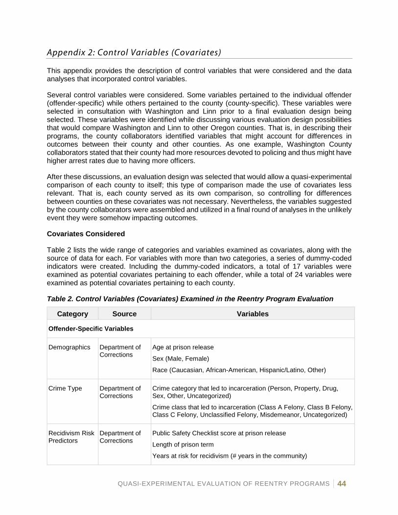
QUASI-EXPERIMENTAL EVALUATION OF REENTRY PROGRAMS 44
Appendix 2: Control Variables (Covariates)
This appendix provides the description of control variables that were considered and the data analyses that incorporated control variables.
Several control variables were considered. Some variables pertained to the individual offender (offender-specific) while others pertained to the county (county-specific). These variables were selected in consultation with Washington and Linn prior to a final evaluation design being selected. These variables were identified while discussing various evaluation design possibilities that would compare Washington and Linn to other Oregon counties. That is, in describing their programs, the county collaborators identified variables that might account for differences in outcomes between their county and other counties. As one example, Washington County collaborators stated that their county had more resources devoted to policing and thus might have higher arrest rates due to having more officers.
After these discussions, an evaluation design was selected that would allow a quasi-experimental comparison of each county to itself; this type of comparison made the use of covariates less relevant. That is, each county served as its own comparison, so controlling for differences between counties on these covariates was not necessary. Nevertheless, the variables suggested by the county collaborators were assembled and utilized in a final round of analyses in the unlikely event they were somehow impacting outcomes.
Covariates Considered
Table 2 lists the wide range of categories and variables examined as covariates, along with the source of data for each. For variables with more than two categories, a series of dummy-coded indicators were created. Including the dummy-coded indicators, a total of 17 variables were examined as potential covariates pertaining to each offender, while a total of 24 variables were examined as potential covariates pertaining to each county.
Table 2. Control Variables (Covariates) Examined in the Reentry Program Evaluation
Category Source Variables
Offender-Specific Variables
Demographics Department of Corrections
Age at prison release
Sex (Male, Female)
Race (Caucasian, African-American, Hispanic/Latino, Other)
Crime Type Department of Corrections
Crime category that led to incarceration (Person, Property, Drug, Sex, Other, Uncategorized)
Crime class that led to incarceration (Class A Felony, Class B Felony, Class C Felony, Unclassified Felony, Misdemeanor, Uncategorized)
Recidivism Risk Predictors
Department of Corrections
Public Safety Checklist score at prison release
Length of prison term
Years at risk for recidivism (# years in the community)
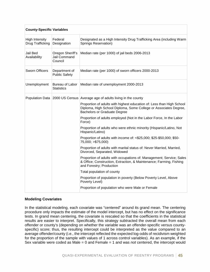
QUASI-EXPERIMENTAL EVALUATION OF REENTRY PROGRAMS 45
County-Specific Variables
High Intensity Drug Trafficking
Federal Designation
Designated as a High Intensity Drug Trafficking Area (including Warm Springs Reservation)
Jail Bed Availability
Oregon Sheriff’s Jail Command Council
Median rate (per 1000) of jail beds 2006-2013
Sworn Officers Department of Public Safety
Median rate (per 1000) of sworn officers 2000-2013
Unemployment Bureau of Labor Statistics
Median rate of unemployment 2000-2013
Population Data 2000 US Census Average age of adults living in the county
Proportion of adults with highest education of: Less than High School Diploma, High School Diploma, Some College or Associates Degree, Bachelors or Graduate Degree
Proportion of adults employed (Not in the Labor Force, In the Labor Force)
Proportion of adults who were ethnic minority (Hispanic/Latino, Not Hispanic/Latino)
Proportion of adults with income of: <$25,000; $25-$50,000; $50-75,000; >$75,000)
Proportion of adults with marital status of: Never Married, Married, Divorced, Separated, Widowed
Proportion of adults with occupations of: Management; Service; Sales & Office; Construction, Extraction, & Maintenance; Farming, Fishing and Forestry; Production
Total population of county
Proportion of population in poverty (Below Poverty Level, Above Poverty Level)
Proportion of population who were Male or Female
Modeling Covariates
In the statistical modeling, each covariate was “centered” around its grand mean. The centering procedure only impacts the estimate of the model intercept, but has no effect on the significance tests. In grand mean centering, the covariate is rescaled so that the coefficients in the statistical results are easier to interpret. Specifically, this strategy subtracted the overall mean from each offender or county’s (depending on whether the variable was an offender-specific versus county-specific) score; thus, the resulting intercept could be interpreted as the value compared to an average offender/county (i.e., the intercept reflected the expected log-odds of recidivism weighted for the proportion of the sample with values of 1 across control variables). As an example, if the Sex variable were coded as Male = 0 and Female = 1 and was not centered, the intercept would
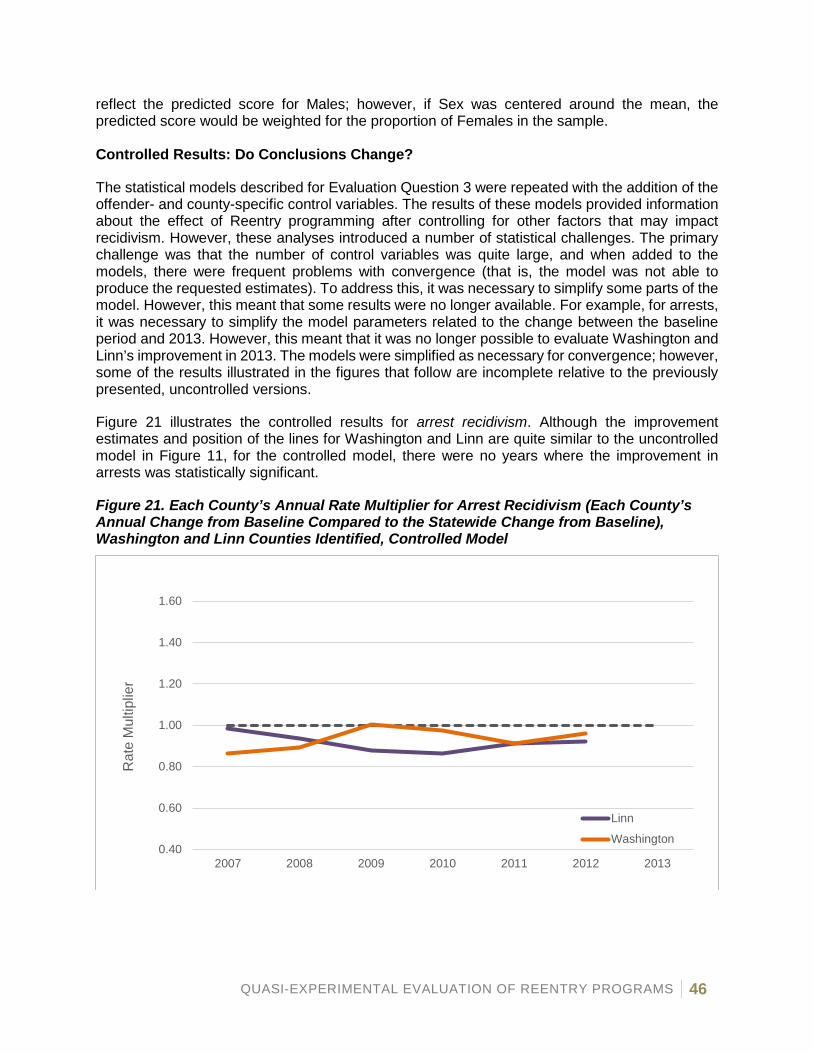
QUASI-EXPERIMENTAL EVALUATION OF REENTRY PROGRAMS 46
reflect the predicted score for Males; however, if Sex was centered around the mean, the predicted score would be weighted for the proportion of Females in the sample. Controlled Results: Do Conclusions Change?
The statistical models described for Evaluation Question 3 were repeated with the addition of the offender- and county-specific control variables. The results of these models provided information about the effect of Reentry programming after controlling for other factors that may impact recidivism. However, these analyses introduced a number of statistical challenges. The primary challenge was that the number of control variables was quite large, and when added to the models, there were frequent problems with convergence (that is, the model was not able to produce the requested estimates). To address this, it was necessary to simplify some parts of the model. However, this meant that some results were no longer available. For example, for arrests, it was necessary to simplify the model parameters related to the change between the baseline period and 2013. However, this meant that it was no longer possible to evaluate Washington and Linn’s improvement in 2013. The models were simplified as necessary for convergence; however, some of the results illustrated in the figures that follow are incomplete relative to the previously presented, uncontrolled versions.
Figure 21 illustrates the controlled results for arrest recidivism. Although the improvement estimates and position of the lines for Washington and Linn are quite similar to the uncontrolled model in Figure 11, for the controlled model, there were no years where the improvement in arrests was statistically significant.
Figure 21. Each County’s Annual Rate Multiplier for Arrest Recidivism (Each County’s Annual Change from Baseline Compared to the Statewide Change from Baseline), Washington and Linn Counties Identified, Controlled Model
0.40
0.60
0.80
1.00
1.20
1.40
1.60
2007 2008 2009 2010 2011 2012 2013
Rat
e M
ultip
lier
Linn
Washington
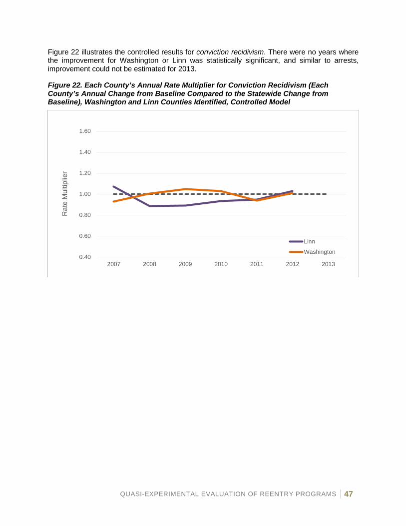
QUASI-EXPERIMENTAL EVALUATION OF REENTRY PROGRAMS 47
Figure 22 illustrates the controlled results for conviction recidivism. There were no years where the improvement for Washington or Linn was statistically significant, and similar to arrests, improvement could not be estimated for 2013.
Figure 22. Each County’s Annual Rate Multiplier for Conviction Recidivism (Each County’s Annual Change from Baseline Compared to the Statewide Change from Baseline), Washington and Linn Counties Identified, Controlled Model
0.40
0.60
0.80
1.00
1.20
1.40
1.60
2007 2008 2009 2010 2011 2012 2013
Rat
e M
ultip
lier
Linn
Washington

QUASI-EXPERIMENTAL EVALUATION OF REENTRY PROGRAMS 48
Figure 23 illustrates the results for incarceration recidivism. There were no years where the improvement for Washington or Linn was statistically significant, and the improvement for years 2007 and 2013 could not be estimated.
Figure 23. Each County’s Annual Rate Multiplier for Incarceration Recidivism (Each County’s Annual Change from Baseline Compared to the Statewide Change from Baseline), Washington and Linn Counties Identified, Controlled Model
Summary of Controlled Results
Significant findings disappeared when covariates were considered in the models. However, and as noted previously, because the evaluation design involved comparison of each county to itself at an earlier point in time, the concept of controlling for covariates is less relevant. Initially, other designs were considered in which Washington and Linn Counties would have been compared to other similar counties; for those designs, covariates would have been desirable to account for the effects of potential county differences. But, the final selected design in which each county was compared to itself resulted in the covariates being less germane to the evaluation.
0.40
0.60
0.80
1.00
1.20
1.40
1.60
2007 2008 2009 2010 2011 2012 2013
Rat
e M
ultip
lier
LinnWashington
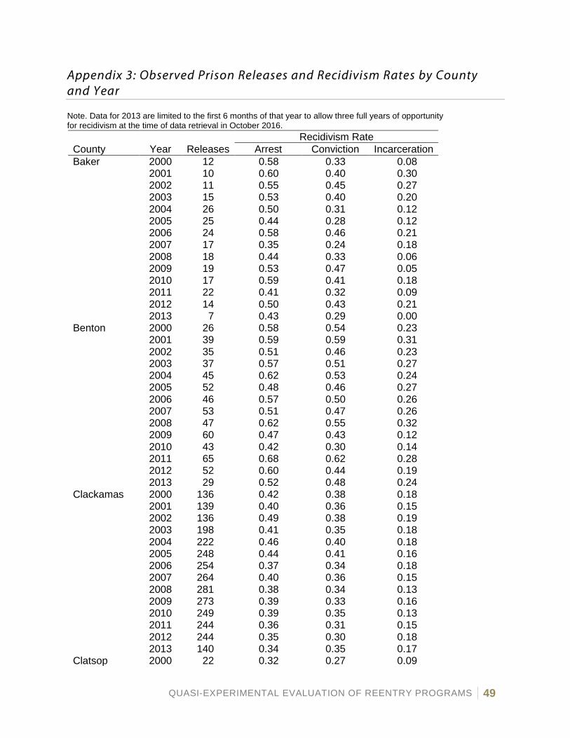
QUASI-EXPERIMENTAL EVALUATION OF REENTRY PROGRAMS 49
Appendix 3: Observed Prison Releases and Recidivism Rates by County and Year
Note. Data for 2013 are limited to the first 6 months of that year to allow three full years of opportunity for recidivism at the time of data retrieval in October 2016.
Recidivism Rate County Year Releases Arrest Conviction Incarceration Baker 2000 12 0.58 0.33 0.08
2001 10 0.60 0.40 0.30 2002 11 0.55 0.45 0.27 2003 15 0.53 0.40 0.20 2004 26 0.50 0.31 0.12 2005 25 0.44 0.28 0.12 2006 24 0.58 0.46 0.21 2007 17 0.35 0.24 0.18 2008 18 0.44 0.33 0.06 2009 19 0.53 0.47 0.05 2010 17 0.59 0.41 0.18 2011 22 0.41 0.32 0.09 2012 14 0.50 0.43 0.21 2013 7 0.43 0.29 0.00
Benton 2000 26 0.58 0.54 0.23 2001 39 0.59 0.59 0.31 2002 35 0.51 0.46 0.23 2003 37 0.57 0.51 0.27 2004 45 0.62 0.53 0.24 2005 52 0.48 0.46 0.27 2006 46 0.57 0.50 0.26 2007 53 0.51 0.47 0.26 2008 47 0.62 0.55 0.32 2009 60 0.47 0.43 0.12 2010 43 0.42 0.30 0.14 2011 65 0.68 0.62 0.28 2012 52 0.60 0.44 0.19 2013 29 0.52 0.48 0.24
Clackamas 2000 136 0.42 0.38 0.18 2001 139 0.40 0.36 0.15 2002 136 0.49 0.38 0.19 2003 198 0.41 0.35 0.18 2004 222 0.46 0.40 0.18 2005 248 0.44 0.41 0.16 2006 254 0.37 0.34 0.18 2007 264 0.40 0.36 0.15 2008 281 0.38 0.34 0.13 2009 273 0.39 0.33 0.16 2010 249 0.39 0.35 0.13 2011 244 0.36 0.31 0.15 2012 244 0.35 0.30 0.18 2013 140 0.34 0.35 0.17
Clatsop 2000 22 0.32 0.27 0.09
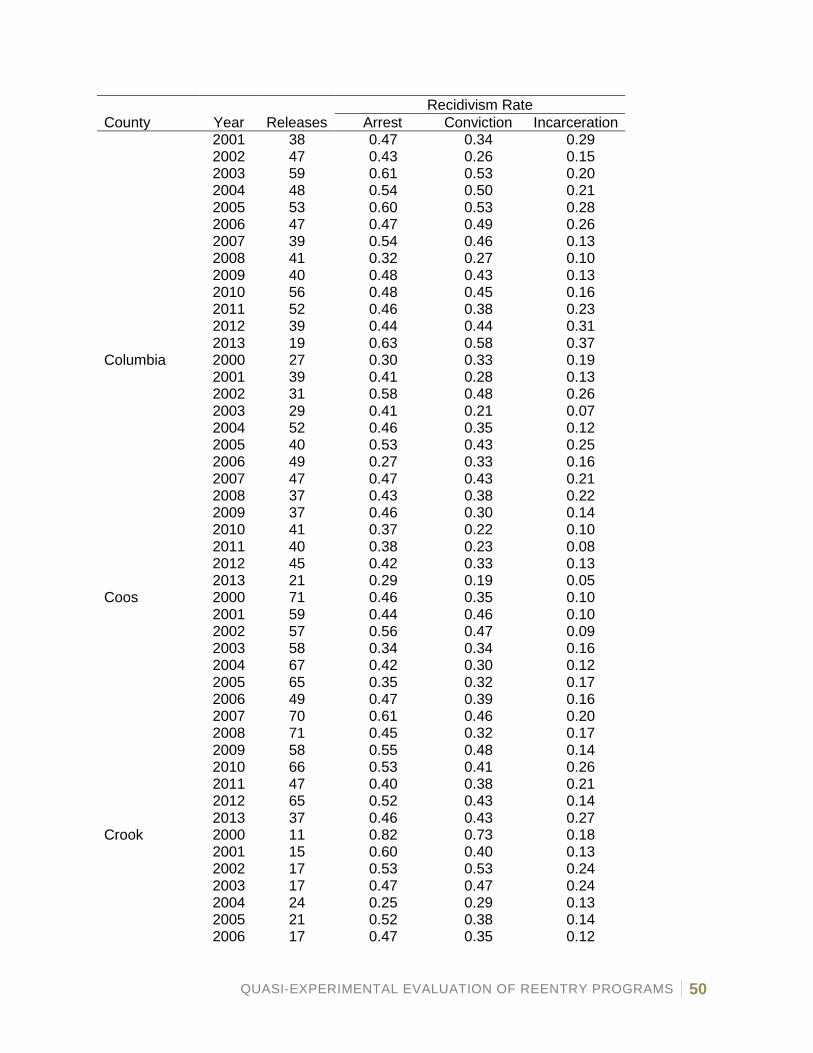
QUASI-EXPERIMENTAL EVALUATION OF REENTRY PROGRAMS 50
Recidivism Rate County Year Releases Arrest Conviction Incarceration
2001 38 0.47 0.34 0.29 2002 47 0.43 0.26 0.15 2003 59 0.61 0.53 0.20 2004 48 0.54 0.50 0.21 2005 53 0.60 0.53 0.28 2006 47 0.47 0.49 0.26 2007 39 0.54 0.46 0.13 2008 41 0.32 0.27 0.10 2009 40 0.48 0.43 0.13 2010 56 0.48 0.45 0.16 2011 52 0.46 0.38 0.23 2012 39 0.44 0.44 0.31 2013 19 0.63 0.58 0.37
Columbia 2000 27 0.30 0.33 0.19 2001 39 0.41 0.28 0.13 2002 31 0.58 0.48 0.26 2003 29 0.41 0.21 0.07 2004 52 0.46 0.35 0.12 2005 40 0.53 0.43 0.25 2006 49 0.27 0.33 0.16 2007 47 0.47 0.43 0.21 2008 37 0.43 0.38 0.22 2009 37 0.46 0.30 0.14 2010 41 0.37 0.22 0.10 2011 40 0.38 0.23 0.08 2012 45 0.42 0.33 0.13 2013 21 0.29 0.19 0.05
Coos 2000 71 0.46 0.35 0.10 2001 59 0.44 0.46 0.10 2002 57 0.56 0.47 0.09 2003 58 0.34 0.34 0.16 2004 67 0.42 0.30 0.12 2005 65 0.35 0.32 0.17 2006 49 0.47 0.39 0.16 2007 70 0.61 0.46 0.20 2008 71 0.45 0.32 0.17 2009 58 0.55 0.48 0.14 2010 66 0.53 0.41 0.26 2011 47 0.40 0.38 0.21 2012 65 0.52 0.43 0.14 2013 37 0.46 0.43 0.27
Crook 2000 11 0.82 0.73 0.18 2001 15 0.60 0.40 0.13 2002 17 0.53 0.53 0.24 2003 17 0.47 0.47 0.24 2004 24 0.25 0.29 0.13 2005 21 0.52 0.38 0.14 2006 17 0.47 0.35 0.12
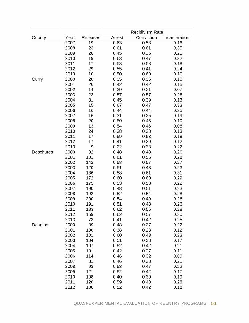
QUASI-EXPERIMENTAL EVALUATION OF REENTRY PROGRAMS 51
Recidivism Rate County Year Releases Arrest Conviction Incarceration
2007 19 0.63 0.58 0.16 2008 23 0.61 0.61 0.35 2009 20 0.45 0.35 0.20 2010 19 0.63 0.47 0.32 2011 17 0.53 0.53 0.18 2012 29 0.55 0.41 0.24 2013 10 0.50 0.60 0.10
Curry 2000 20 0.35 0.35 0.10 2001 26 0.42 0.42 0.15 2002 14 0.29 0.21 0.07 2003 23 0.57 0.57 0.26 2004 31 0.45 0.39 0.13 2005 15 0.67 0.47 0.33 2006 16 0.44 0.44 0.25 2007 16 0.31 0.25 0.19 2008 20 0.50 0.45 0.10 2009 13 0.54 0.46 0.08 2010 24 0.38 0.38 0.13 2011 17 0.59 0.53 0.18 2012 17 0.41 0.29 0.12 2013 9 0.22 0.33 0.22
Deschutes 2000 82 0.48 0.43 0.26 2001 101 0.61 0.56 0.28 2002 142 0.58 0.57 0.27 2003 120 0.51 0.43 0.23 2004 136 0.58 0.61 0.31 2005 172 0.60 0.60 0.29 2006 175 0.53 0.53 0.22 2007 190 0.48 0.51 0.23 2008 192 0.52 0.54 0.28 2009 200 0.54 0.49 0.26 2010 191 0.51 0.43 0.26 2011 183 0.62 0.55 0.28 2012 169 0.62 0.57 0.30 2013 73 0.41 0.42 0.25
Douglas 2000 89 0.48 0.37 0.22 2001 100 0.38 0.28 0.12 2002 101 0.60 0.43 0.23 2003 104 0.51 0.38 0.17 2004 107 0.52 0.42 0.21 2005 101 0.42 0.27 0.11 2006 114 0.46 0.32 0.09 2007 81 0.46 0.33 0.21 2008 93 0.53 0.47 0.22 2009 121 0.52 0.42 0.17 2010 108 0.40 0.30 0.19 2011 120 0.59 0.48 0.28 2012 106 0.52 0.42 0.18

QUASI-EXPERIMENTAL EVALUATION OF REENTRY PROGRAMS 52
Recidivism Rate County Year Releases Arrest Conviction Incarceration
2013 68 0.56 0.40 0.18 Gilliam 2000 0 2001 0 2002 0 2003 2 0.00 0.00 0.00
2004 1 1.00 1.00 1.00 2005 2 0.00 0.00 0.00 2006 2 0.50 0.50 0.50 2007 3 0.67 0.67 0.00 2008 1 0.00 0.00 0.00 2009 2 0.50 0.50 0.00 2010 0 2011 3 0.33 0.00 0.00
2012 0 2013 0 Grant 2000 2 0.00 0.00 0.00
2001 1 0.00 0.00 0.00 2002 3 1.00 0.67 0.00 2003 0 2004 3 0.33 0.33 0.33 2005 6 0.33 0.33 0.17 2006 2 0.50 0.50 0.00 2007 1 0.00 0.00 0.00 2008 3 0.00 0.00 0.00 2009 3 0.33 0.00 0.00 2010 3 0.33 0.00 0.00 2011 5 0.40 0.40 0.00 2012 7 0.43 0.29 0.14 2013 1 1.00 1.00 0.00
Harney 2000 2 1.00 0.50 0.50 2001 8 0.63 0.50 0.38 2002 4 0.25 0.25 0.25 2003 8 0.63 0.63 0.50 2004 16 0.56 0.50 0.13 2005 15 0.53 0.47 0.27 2006 7 0.29 0.14 0.14 2007 14 0.43 0.29 0.14 2008 11 0.45 0.36 0.27 2009 14 0.57 0.43 0.36 2010 5 0.40 0.20 0.20 2011 16 0.25 0.13 0.00 2012 16 0.31 0.25 0.13 2013 6 0.33 0.17 0.17
Hood River 2000 7 0.29 0.14 0.00 2001 10 0.30 0.30 0.20 2002 10 0.40 0.30 0.10 2003 16 0.19 0.06 0.00 2004 7 0.14 0.14 0.00
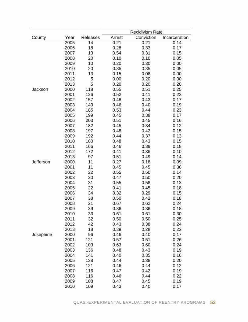
QUASI-EXPERIMENTAL EVALUATION OF REENTRY PROGRAMS 53
Recidivism Rate County Year Releases Arrest Conviction Incarceration
2005 14 0.21 0.21 0.14 2006 18 0.28 0.33 0.17 2007 13 0.54 0.31 0.15 2008 20 0.10 0.10 0.05 2009 10 0.20 0.30 0.00 2010 20 0.35 0.35 0.05 2011 13 0.15 0.08 0.00 2012 5 0.00 0.20 0.00 2013 5 0.20 0.20 0.20
Jackson 2000 118 0.55 0.51 0.25 2001 126 0.52 0.41 0.23 2002 157 0.48 0.43 0.17 2003 140 0.46 0.40 0.19 2004 185 0.53 0.44 0.23 2005 199 0.45 0.39 0.17 2006 203 0.51 0.45 0.16 2007 182 0.45 0.34 0.12 2008 197 0.48 0.42 0.15 2009 192 0.44 0.37 0.13 2010 160 0.48 0.43 0.15 2011 166 0.46 0.39 0.18 2012 172 0.41 0.36 0.10 2013 97 0.51 0.49 0.14
Jefferson 2000 11 0.27 0.18 0.09 2001 11 0.45 0.45 0.36 2002 22 0.55 0.50 0.14 2003 30 0.47 0.50 0.20 2004 31 0.55 0.58 0.13 2005 22 0.41 0.45 0.18 2006 34 0.32 0.29 0.15 2007 38 0.50 0.42 0.18 2008 21 0.67 0.62 0.24 2009 39 0.36 0.36 0.18 2010 33 0.61 0.61 0.30 2011 32 0.50 0.50 0.25 2012 42 0.43 0.38 0.24 2013 18 0.39 0.28 0.22
Josephine 2000 96 0.46 0.40 0.17 2001 121 0.57 0.51 0.26 2002 103 0.63 0.60 0.24 2003 136 0.48 0.43 0.19 2004 141 0.40 0.35 0.16 2005 138 0.44 0.38 0.20 2006 121 0.46 0.44 0.12 2007 116 0.47 0.42 0.19 2008 116 0.46 0.44 0.22 2009 108 0.47 0.45 0.19 2010 109 0.43 0.40 0.17
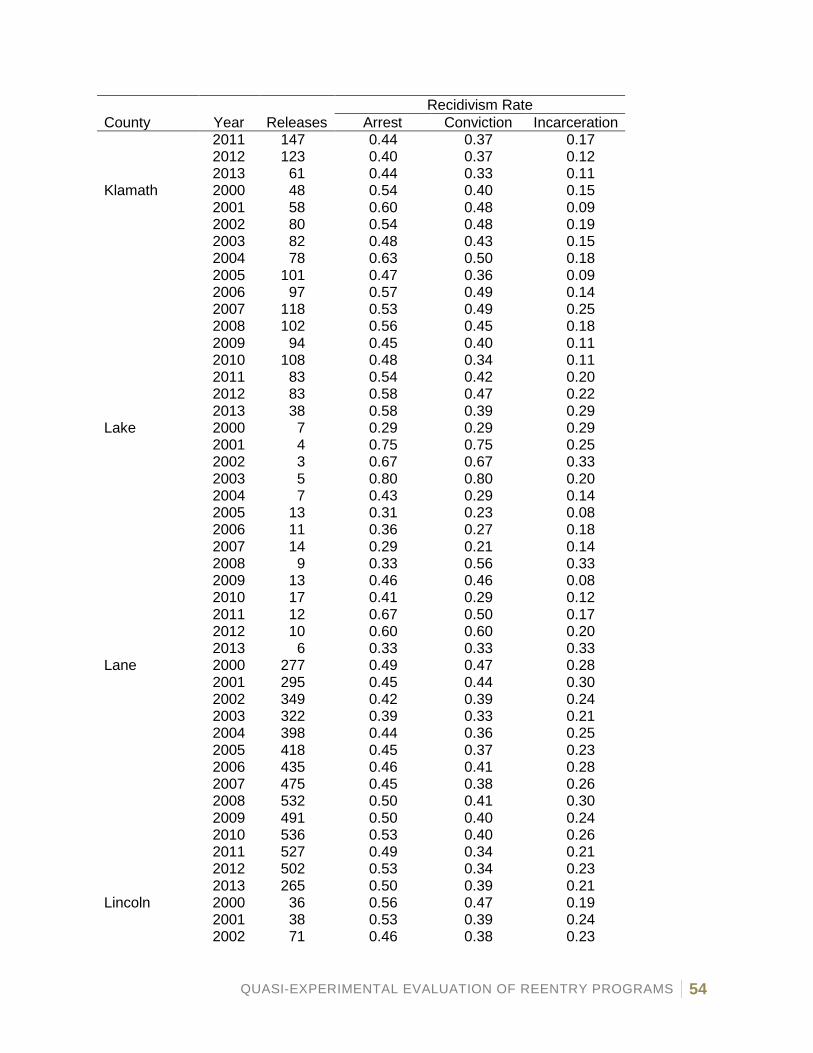
QUASI-EXPERIMENTAL EVALUATION OF REENTRY PROGRAMS 54
Recidivism Rate County Year Releases Arrest Conviction Incarceration
2011 147 0.44 0.37 0.17 2012 123 0.40 0.37 0.12 2013 61 0.44 0.33 0.11
Klamath 2000 48 0.54 0.40 0.15 2001 58 0.60 0.48 0.09 2002 80 0.54 0.48 0.19 2003 82 0.48 0.43 0.15 2004 78 0.63 0.50 0.18 2005 101 0.47 0.36 0.09 2006 97 0.57 0.49 0.14 2007 118 0.53 0.49 0.25 2008 102 0.56 0.45 0.18 2009 94 0.45 0.40 0.11 2010 108 0.48 0.34 0.11 2011 83 0.54 0.42 0.20 2012 83 0.58 0.47 0.22 2013 38 0.58 0.39 0.29
Lake 2000 7 0.29 0.29 0.29 2001 4 0.75 0.75 0.25 2002 3 0.67 0.67 0.33 2003 5 0.80 0.80 0.20 2004 7 0.43 0.29 0.14 2005 13 0.31 0.23 0.08 2006 11 0.36 0.27 0.18 2007 14 0.29 0.21 0.14 2008 9 0.33 0.56 0.33 2009 13 0.46 0.46 0.08 2010 17 0.41 0.29 0.12 2011 12 0.67 0.50 0.17 2012 10 0.60 0.60 0.20 2013 6 0.33 0.33 0.33
Lane 2000 277 0.49 0.47 0.28 2001 295 0.45 0.44 0.30 2002 349 0.42 0.39 0.24 2003 322 0.39 0.33 0.21 2004 398 0.44 0.36 0.25 2005 418 0.45 0.37 0.23 2006 435 0.46 0.41 0.28 2007 475 0.45 0.38 0.26 2008 532 0.50 0.41 0.30 2009 491 0.50 0.40 0.24 2010 536 0.53 0.40 0.26 2011 527 0.49 0.34 0.21 2012 502 0.53 0.34 0.23 2013 265 0.50 0.39 0.21
Lincoln 2000 36 0.56 0.47 0.19 2001 38 0.53 0.39 0.24 2002 71 0.46 0.38 0.23

QUASI-EXPERIMENTAL EVALUATION OF REENTRY PROGRAMS 55
Recidivism Rate County Year Releases Arrest Conviction Incarceration
2003 58 0.43 0.33 0.17 2004 61 0.44 0.38 0.15 2005 53 0.58 0.47 0.21 2006 72 0.50 0.54 0.15 2007 72 0.47 0.42 0.24 2008 56 0.38 0.36 0.16 2009 57 0.46 0.40 0.16 2010 55 0.45 0.40 0.15 2011 53 0.55 0.45 0.11 2012 61 0.48 0.39 0.20 2013 25 0.60 0.44 0.28
Linn 2000 106 0.63 0.56 0.39 2001 118 0.57 0.47 0.23 2002 142 0.61 0.55 0.32 2003 154 0.62 0.55 0.34 2004 157 0.54 0.50 0.40 2005 197 0.60 0.55 0.37 2006 183 0.50 0.44 0.30 2007 195 0.55 0.52 0.33 2008 183 0.52 0.46 0.31 2009 255 0.50 0.41 0.23 2010 203 0.52 0.45 0.26 2011 208 0.46 0.38 0.25 2012 197 0.53 0.46 0.25 2013 78 0.46 0.41 0.29
Malheur 2000 53 0.43 0.34 0.11 2001 50 0.16 0.22 0.10 2002 43 0.42 0.33 0.16 2003 59 0.25 0.24 0.12 2004 51 0.33 0.35 0.22 2005 37 0.30 0.24 0.14 2006 52 0.48 0.44 0.23 2007 54 0.41 0.39 0.15 2008 34 0.26 0.15 0.09 2009 59 0.37 0.34 0.14 2010 50 0.30 0.28 0.20 2011 36 0.33 0.22 0.08 2012 46 0.35 0.41 0.15 2013 12 0.58 0.42 0.17
Marion 2000 290 0.47 0.43 0.25 2001 377 0.54 0.45 0.26 2002 452 0.49 0.44 0.26 2003 511 0.48 0.41 0.26 2004 612 0.55 0.47 0.27 2005 659 0.54 0.42 0.23 2006 699 0.48 0.40 0.23 2007 628 0.50 0.42 0.24 2008 641 0.48 0.41 0.21

QUASI-EXPERIMENTAL EVALUATION OF REENTRY PROGRAMS 56
Recidivism Rate County Year Releases Arrest Conviction Incarceration
2009 667 0.41 0.36 0.20 2010 617 0.40 0.33 0.20 2011 597 0.45 0.40 0.25 2012 565 0.42 0.39 0.23 2013 280 0.45 0.41 0.23
Morrow 2000 1 1.00 1.00 1.00 2001 3 0.67 0.33 0.00 2002 1 0.00 1.00 1.00 2003 1 1.00 1.00 0.00 2004 2 1.00 1.00 0.00 2005 5 0.80 0.60 0.20 2006 1 1.00 0.00 0.00 2007 8 0.25 0.25 0.00 2008 3 0.00 0.00 0.00 2009 3 1.00 0.67 0.33 2010 2 0.00 0.00 0.00 2011 13 0.54 0.15 0.08 2012 6 0.50 0.33 0.00 2013 1 0.00 0.00 0.00
Multnomah 2000 1022 0.50 0.45 0.22 2001 986 0.47 0.42 0.20 2002 1110 0.49 0.44 0.20 2003 1126 0.47 0.44 0.20 2004 1086 0.50 0.44 0.21 2005 1063 0.48 0.47 0.22 2006 1107 0.49 0.46 0.23 2007 1082 0.47 0.45 0.22 2008 1088 0.49 0.48 0.21 2009 1216 0.44 0.42 0.20 2010 1180 0.47 0.45 0.23 2011 1123 0.45 0.42 0.19 2012 1043 0.48 0.44 0.20 2013 490 0.48 0.41 0.20
Polk 2000 26 0.42 0.27 0.04 2001 32 0.38 0.28 0.16 2002 43 0.56 0.35 0.30 2003 39 0.38 0.28 0.18 2004 55 0.51 0.44 0.24 2005 60 0.58 0.47 0.25 2006 37 0.35 0.35 0.19 2007 65 0.43 0.38 0.22 2008 55 0.36 0.31 0.20 2009 69 0.38 0.38 0.12 2010 58 0.45 0.41 0.12 2011 49 0.43 0.29 0.10 2012 64 0.50 0.50 0.31 2013 26 0.50 0.50 0.19
Sherman 2000 1 0.00 0.00 0.00
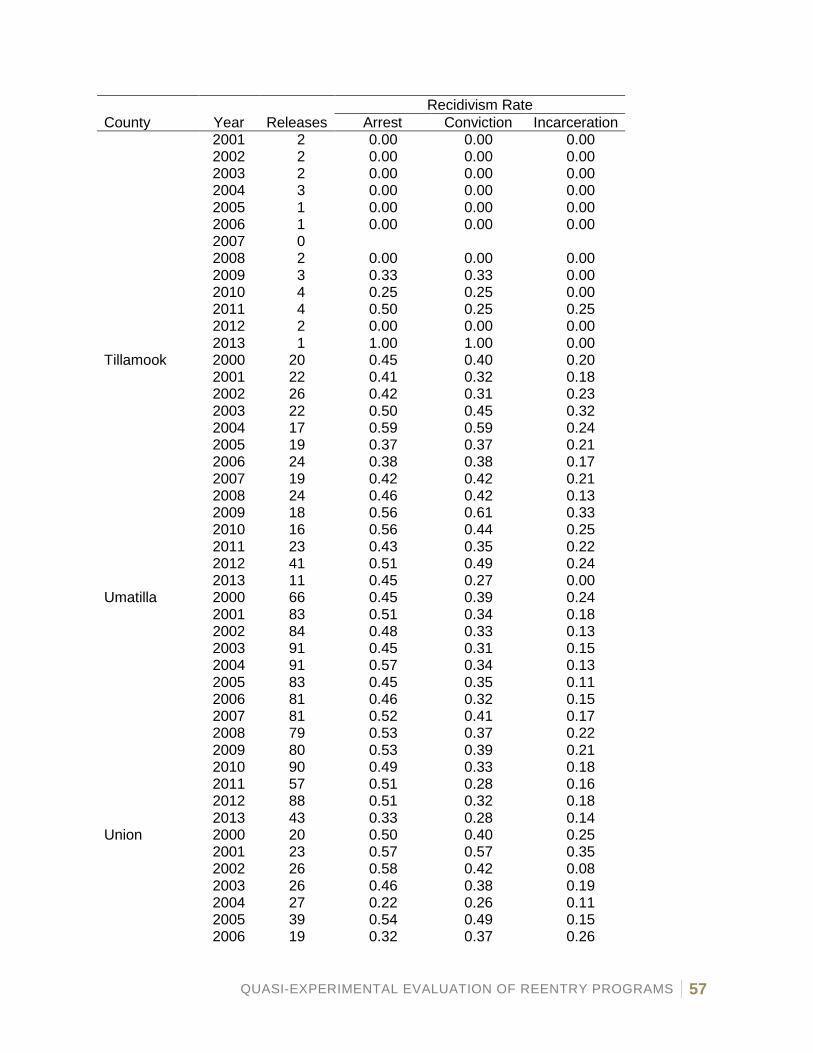
QUASI-EXPERIMENTAL EVALUATION OF REENTRY PROGRAMS 57
Recidivism Rate County Year Releases Arrest Conviction Incarceration
2001 2 0.00 0.00 0.00 2002 2 0.00 0.00 0.00 2003 2 0.00 0.00 0.00 2004 3 0.00 0.00 0.00 2005 1 0.00 0.00 0.00 2006 1 0.00 0.00 0.00 2007 0 2008 2 0.00 0.00 0.00 2009 3 0.33 0.33 0.00 2010 4 0.25 0.25 0.00 2011 4 0.50 0.25 0.25 2012 2 0.00 0.00 0.00 2013 1 1.00 1.00 0.00
Tillamook 2000 20 0.45 0.40 0.20 2001 22 0.41 0.32 0.18 2002 26 0.42 0.31 0.23 2003 22 0.50 0.45 0.32 2004 17 0.59 0.59 0.24 2005 19 0.37 0.37 0.21 2006 24 0.38 0.38 0.17 2007 19 0.42 0.42 0.21 2008 24 0.46 0.42 0.13 2009 18 0.56 0.61 0.33 2010 16 0.56 0.44 0.25 2011 23 0.43 0.35 0.22 2012 41 0.51 0.49 0.24 2013 11 0.45 0.27 0.00
Umatilla 2000 66 0.45 0.39 0.24 2001 83 0.51 0.34 0.18 2002 84 0.48 0.33 0.13 2003 91 0.45 0.31 0.15 2004 91 0.57 0.34 0.13 2005 83 0.45 0.35 0.11 2006 81 0.46 0.32 0.15 2007 81 0.52 0.41 0.17 2008 79 0.53 0.37 0.22 2009 80 0.53 0.39 0.21 2010 90 0.49 0.33 0.18 2011 57 0.51 0.28 0.16 2012 88 0.51 0.32 0.18 2013 43 0.33 0.28 0.14
Union 2000 20 0.50 0.40 0.25 2001 23 0.57 0.57 0.35 2002 26 0.58 0.42 0.08 2003 26 0.46 0.38 0.19 2004 27 0.22 0.26 0.11 2005 39 0.54 0.49 0.15 2006 19 0.32 0.37 0.26
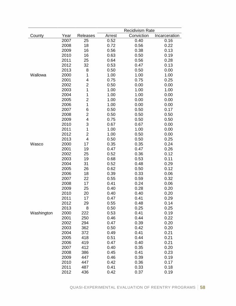
QUASI-EXPERIMENTAL EVALUATION OF REENTRY PROGRAMS 58
Recidivism Rate County Year Releases Arrest Conviction Incarceration
2007 25 0.52 0.40 0.16 2008 18 0.72 0.56 0.22 2009 16 0.56 0.38 0.13 2010 16 0.63 0.50 0.19 2011 25 0.64 0.56 0.28 2012 32 0.53 0.47 0.13 2013 8 0.50 0.50 0.00
Wallowa 2000 1 1.00 1.00 1.00 2001 4 0.75 0.75 0.25 2002 2 0.50 0.00 0.00 2003 1 1.00 1.00 1.00 2004 1 1.00 1.00 0.00 2005 2 1.00 0.00 0.00 2006 1 1.00 0.00 0.00 2007 6 0.50 0.50 0.17 2008 2 0.50 0.50 0.50 2009 4 0.75 0.50 0.50 2010 3 0.67 0.67 0.00 2011 1 1.00 1.00 0.00 2012 2 1.00 0.50 0.00 2013 4 0.50 0.50 0.25
Wasco 2000 17 0.35 0.35 0.24 2001 19 0.47 0.47 0.26 2002 25 0.52 0.36 0.12 2003 19 0.68 0.53 0.11 2004 31 0.52 0.48 0.29 2005 26 0.62 0.50 0.12 2006 18 0.39 0.33 0.06 2007 22 0.55 0.59 0.32 2008 17 0.41 0.24 0.06 2009 25 0.40 0.28 0.20 2010 20 0.40 0.40 0.20 2011 17 0.47 0.41 0.29 2012 29 0.55 0.48 0.14 2013 8 0.50 0.25 0.25
Washington 2000 222 0.53 0.41 0.19 2001 250 0.46 0.44 0.22 2002 294 0.47 0.39 0.20 2003 362 0.50 0.42 0.20 2004 372 0.49 0.41 0.21 2005 418 0.51 0.44 0.21 2006 419 0.47 0.40 0.21 2007 412 0.40 0.35 0.20 2008 386 0.45 0.41 0.23 2009 447 0.46 0.39 0.19 2010 447 0.42 0.36 0.17 2011 487 0.41 0.33 0.18 2012 436 0.42 0.37 0.19
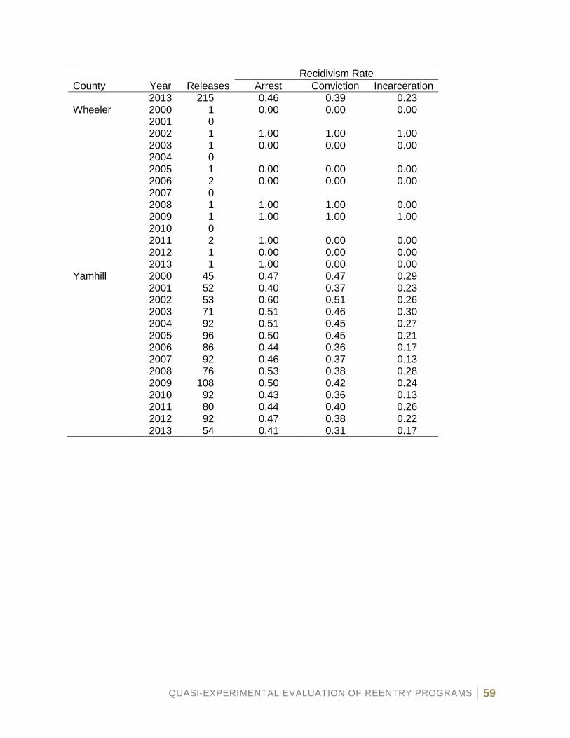
QUASI-EXPERIMENTAL EVALUATION OF REENTRY PROGRAMS 59
Recidivism Rate County Year Releases Arrest Conviction Incarceration
2013 215 0.46 0.39 0.23 Wheeler 2000 1 0.00 0.00 0.00
2001 0 2002 1 1.00 1.00 1.00 2003 1 0.00 0.00 0.00 2004 0 2005 1 0.00 0.00 0.00 2006 2 0.00 0.00 0.00 2007 0 2008 1 1.00 1.00 0.00 2009 1 1.00 1.00 1.00 2010 0 2011 2 1.00 0.00 0.00 2012 1 0.00 0.00 0.00 2013 1 1.00 0.00 0.00
Yamhill 2000 45 0.47 0.47 0.29 2001 52 0.40 0.37 0.23 2002 53 0.60 0.51 0.26 2003 71 0.51 0.46 0.30 2004 92 0.51 0.45 0.27 2005 96 0.50 0.45 0.21 2006 86 0.44 0.36 0.17 2007 92 0.46 0.37 0.13 2008 76 0.53 0.38 0.28 2009 108 0.50 0.42 0.24 2010 92 0.43 0.36 0.13 2011 80 0.44 0.40 0.26 2012 92 0.47 0.38 0.22 2013 54 0.41 0.31 0.17