quasi-interpretation synthesis by decomposition: an
TRANSCRIPT

HAL Id: inria-00130920https://hal.inria.fr/inria-00130920
Submitted on 14 Feb 2007
HAL is a multi-disciplinary open accessarchive for the deposit and dissemination of sci-entific research documents, whether they are pub-lished or not. The documents may come fromteaching and research institutions in France orabroad, or from public or private research centers.
L’archive ouverte pluridisciplinaire HAL, estdestinée au dépôt et à la diffusion de documentsscientifiques de niveau recherche, publiés ou non,émanant des établissements d’enseignement et derecherche français ou étrangers, des laboratoirespublics ou privés.
Quasi-interpretation Synthesis by Decomposition : Anapplication to higher-order programs
Guillaume Bonfante, Jean-Yves Marion, Romain Péchoux
To cite this version:Guillaume Bonfante, Jean-Yves Marion, Romain Péchoux. Quasi-interpretation Synthesis by Decom-position : An application to higher-order programs. ICTAC, Sep 2007, Macao, China. �inria-00130920�

Modularity of the Quasi-interpretationsSynthesis and an Application to Higher-Order
Programs
Guillaume Bonfante, Jean-Yves Marion and Romain Pechoux
Nancy-Universite, Loria, Carte team, B.P. 239, 54506 Vandœuvre-les-Nancy Cedex,France, and Ecole Nationale Superieure des Mines de Nancy, INPL, France.
[email protected] [email protected]
Abstract. Quasi-interpretations have shown their interest to deal withresource analysis of first order functional programs. There are at leasttwo reasons to study the question of modularity of quasi-interpretations.Firstly, modularity allows to decrease the complexity of the quasi-inter-pretation search algorithms. Secondly, modularity allows to increase theintentionality of the quasi-interpretation method, that is the number ofcaptured programs. In particular, we take advantage of modularity condi-tions to extend smoothly quasi-interpretations to higher order programs.In this paper, we study the modularity of quasi-interpretations throughthe notions of constructor-sharing and hierarchical unions. We show thatin the case of constructor-sharing and hierarchical unions, the existenceof quasi-interpretations is no longer a modular property. However, wecan still certify the complexity of programs.
1 Introduction
1.1 Certifying resources by Quasi-interpretations
The control of resource (i.e. memory/space or time) is a fundamental issue forcritical systems. The present work, which considers more specifically the staticanalysis of first order functional programs, is a contribution to that field and, inparticular, to the field of implicit computational complexity (ICC).
We briefly review four distinct approaches to that issue of the (ICC) com-munity. The first one deals with linear type disciplines in order to restrict com-putational time and began with the seminal work of Girard [18] which definedLight Linear Logic. The interested reader should consult the recent results ofBaillot-Terui [5], Lafont [28] and Coppola-Ronchi [13]. The second approach isdue to Hofmann [21, 22, 4], who introduced a resource atomic type, into lineartype systems, for higher-order functional programming. The third one consid-ers imperative programming languages and is developed by Jones-Kristianssen,Niggl [35], Marion-Moyen [34, 31]. The fourth approach is the one on which we fo-cus in this paper. It concerns term rewriting systems and quasi-interpretations. Aquasi-interpretation of a first order functional program provides an upper bound

2
on the size of any value computed. The paper [7] is a comprehensive introductionto quasi-interpretations. Combined with recursive path orderings, it allows char-acterizing complexity classes such as the set of polynomial time functions or yetthe set of polynomial space functions. The main features of quasi-interpretations(abbreviated QI) are the following.
1. QI analysis includes a broad class of algorithms, even some that have anexponentially length derivation but denote a polynomial time computablefunction using dynamic programming techniques. See [30, 6, 8]
2. Resource verification of bytecode programs obtained by compiling first orderfunctional and reactive programs which admit quasi-interpretations. See forexample [2, 3, 14].
3. In [9], the synthesis of QI was shown to be decidable in exponential time forpolynomial quasi-interpretations of bounded degree over real numbers.
QI provide a methodology in order to determine and control the involved re-sources in a computation. From a developer perspective, a virtual machine runsand manages codes. We attach to each program a QI. As programs are loaded forexecution, each program has its own QI. So the virtual machine, which executesa program, knows an upper bound on necessary resources and may predict andbe aware of, say, the size of stack frames, which could be of great importancefor execution efficiency.
1.2 Improving QI Synthesis
The problem of the QI synthesis, which was first studied by Amadio in [1], con-sists in finding a QI for a given program. In a perspective of automatic analysisof the complexity of programs, such a problematic is fundamental. The synthesisof QI is a very tricky problem which is undecidable in general. Using Tarski’sresult showing that the theory of real numbers with equality, comparison, sumand product is decidable, we have shown in [9] that the QI synthesis for a pro-gram having n variables, has a time complexity in 2nα
, for some constant α, aslong as we take polynomial quasi-interpretations with degree smaller than anarbitrarily fixed constant. On one hand we have a very general procedure, onthe other hand the procedure has a high cost.
The question of modularity of QI is central as long as one considers a divideand conquer strategy to find QI. Take a program and divide it into k sub-programs having nj variables for j from 1 to k. Then the complexity of the QIsynthesis decreases from 2(
Pkj=1 nj)
α
to∑k
j=1 2nαj , for some constant α. Such
results could allow the improvement of a software called CROCUS that we arecurrently developing and which finds QI using some heuristics.
1.3 A modular approach to program resource analysis
The study of modularity is nowadays a classical approach to solve problems,like confluence or termination, by dividing the problem into smaller parts. Thereader should consult [26, 20, 39, 38, 33, 27] to read an overview on this subject.

3
In this context, we first consider the constructor-sharing case in which func-tions defined by programs share constructors. We show that QI are not modular,except in the special case of disjoint union, but we can use QI in order to predictresource bounds. The consequence is that we are able to analyse the complexityof more programs. Indeed, suppose that a program does not admit a QI. A strat-egy is to cut it into two programs, which just have some constructors in common.Then, we can try to find QI of both sub-programs. We demonstrate that in thiscase we can still determine an upper bound on the amount of resource involvedin a computation. Another consequence is a new characterization of the sets ofpolynomial time functions and of polynomial space functions. The second case isthe hierarchical union, where constructors of one program are defined functionsymbols of another program. Again the fact of admitting a QI is not modular.We use the work of Dershowitz [17] introducing some conditions for ensuringthe modularity of completeness for hierarchical unions and put some syntacticrestriction on the programs considered. Again we are able, under these condi-tions, to analyse resource bounds. These results allow to divide programs in amore flexible fashion. Lastly, the hierarchical union of two programs can be con-sidered as a way to deal with higher-order programs. Up to now, the QI methodonly applies to first order functional programs. A way to deal with higher-orderprograms is to transform a higher-order definition into a hierarchical union ofprograms using higher-order removal methods. Then, modularity is a naturalway to ensure resource complexity.
2 First order functional programming
2.1 Syntax of first order programs
A program is defined formally as a quadruple 〈X , C,F ,R〉 with X ,F and C ofdisjoint sets which represent respectively the variables, the function symbols andthe constructors symbols, and R a finite set of rules defined below:
(Values) T (C) 3 v ::= c | c(v1, · · · , vn)(terms) T (C,F ,X ) 3 t ::= c | x | c(t1, · · · , tn) | f(t1, · · · , tn)(patterns) P 3 p ::= c | x | c(p1, · · · , pn)(rules) R 3 r ::= f(p1, · · · , pn) → t
where x ∈ X , f ∈ F , and c ∈ C.The set of rules induces a rewriting relation→. The relation ∗→ is the reflexive
and transitive closure of →. Throughout, we consider only orthogonal programs,that is, rule patterns are disjoint and linear. So each program is confluent [23].
The domain of computation of a program 〈X , C,F ,R〉 is the constructoralgebra T (C). For each function symbol f ∈ F , the program 〈X , C,F ,R〉 com-putes a partial function JfK : T (C)n → T (C) defined by: JfK(v1, · · · , vn) = w ifff(v1, · · · , vn) ∗→w for all vi ∈ T (C) and w is in T (C). Otherwise JfK(v1, · · · , vn) isundefined. A substitution σ is a mapping from variables to terms and a ground

4
substitution is one which ranges over values of T (C). Observe that values arenormal forms for the program. By extension, given a term t and a ground sub-stitution σ, JtσK = w if tσ
∗→w and w is in T (C).The size |t| of a term t is defined to be the number of symbols of arity strictly
greater than 0 occurring in it.
2.2 Recursive Path orderings
Given a program 〈X , C,F ,R〉, we define a precedence ≥F on function symbolsand its transitive closure that we also note ≥F by f ≥F g if there is a rule ofthe shape f(p1, · · · , pn) → C[g(e1, · · · , em)] with C[�] a context and e1, · · · , em
terms. f ≈F g iff f ≥F g and g ≥F f. f >F g iff f ≥F g and not g ≥F f.We associate to each function symbol f a status st(f) in {p, l} and which
satisfies if f ≈F g then st(f) = st(g). The status indicates how to comparerecursive calls. When st(f) = p, the status of f is said to be product. In thatcase, the arguments are compared with the product extension of≺rpo. Otherwise,the status is said to be lexicographic.
Definition 1. The product extension ≺p and the lexicographic extension ≺l of≺ over sequences are defined by:
– (m1, · · · ,mk) ≺p (n1, · · · , nk) if and only if (i) ∀i ≤ k,mi � ni and (ii)∃j ≤ k such that mj ≺ nj.
– (m1, · · · ,mk) ≺l (n1, · · · , nl) if and only if ∃j such that ∀i < j, mi � ni
and mj ≺ nj
Definition 2 ([16],[25]). Given a precedence �F and a status st, we define therecursive path ordering ≺rpo as follows:
u �rpo tif ∈ F
⋃C
u ≺rpo f(. . . , ti, . . .)
∀i ui ≺rpo f(t1, · · · , tn) g ≺F fg ∈ F
⋃C
g(u1, · · · , um) ≺rpo f(t1, · · · , tn)
(u1, · · · , un) ≺st(f)rpo (t1, · · · , tn) f ≈F g ∀i ui ≺rpo f(t1, · · · , tn)
g(u1, · · · , un) ≺rpo f(t1, · · · , tn)
A program is ordered by ≺rpo if there are a precedence �F and a status st suchthat for each rule l → r, the inequality r ≺rpo l holds.
A program which is ordered by ≺rpo terminates and one of the key point of ourwork (see [29] and [32] for dependency pairs) is to use termination proof as amask to capture algorithmic patterns.
3 Quasi-interpretations
3.1 Definition of Quasi-interpretations
An assignment of a symbol b ∈ F⋃C of arity n is a function LbM : (R+)n → R+.

5
An assignment satisfies the subterm property if for any i = 1, n and anyX1, · · · , Xn in R+, we have
LbM(X1, · · · , Xn) ≥ Xi
An assignment is weakly monotone if for any symbol b, LbM is an increasing(not necessarily strictly) function with respect to each variable. That is, forevery symbol b and all X1, · · · , Xn, Y1, · · · , Yn of R with Xi ≤ Yi, we haveLbM(X1, · · · , Xn) ≤ LbM(Y1, · · · , Yn).
We extend assignment L−M to terms canonically. Given a term t with mvariables, the assignment LtM is a function (R+)m → R+ defined by the rules:
Lb(t1, · · · , tn)M = LbM(Lt1M, · · · , LtnM)LxM = X
where X is a fresh variable ranging over reals.
Definition 3 (Quasi-interpretation). A quasi-interpretation L−M of a pro-gram 〈X , C,F ,R〉 is a weakly monotonic assignment satisfying the subterm prop-erty such that for each rule l → r ∈ R, and for every constructor substitutionσ
LlσM ≥ LrσM
3.2 Polynomial and Additive Quasi-Interpretations
Definition 4. Given a semi-ring K, let Max-Poly{K} be the set of functionsdefined to be constant functions over K, projections, max, +, × and closed bycomposition. An assignment L−M is said to be polynomial if for each symbolb ∈ F
⋃C, LbM is a function in Max-Poly{R+}. A quasi-interpretation L−M is
polynomial if the assignment L−M is polynomial.
Now, say that an assignment of a symbol b of arity n > 0 is additive if
LbM(X1, · · · , Xn) =n∑
i=1
Xi + α with α ≥ 1
An assignment L−M of a program p is additive if L−M is polynomial and eachconstructor symbol of p has an additive assignment. A program is additive if itadmits a quasi-interpretation which is an additive assignment.
Example 1. Consider the program which computes the logarithm function anddescribed by the following rules:
log(0) → 0 half(0) → 0log(S(0)) → 0 half(S(0)) → 0
log(S(S(y))) → S(log(S(half(y)))) half(S(S(y))) → S(half(y))

6
It admits the following additive quasi-interpretation:
L0M = 0LSM(X) = X + 1
LlogM(X) = LhalfM(X) = X
3.3 Key properties
Proposition 1. Assume that L−M is an additive quasi-interpretation of a pro-gram p.
1. For any terms u and v such that u∗→v, we have LuM ≥ LvM
2. There is a constant k such that |t| ≤ LtM ≤ k × |t|.3. For any term u and any constructor term t ∈ T (C), if u
∗→t, we have |t| ≤ LuM.
Proof.
1. A context is a particular term that we write C[�] where � is a new variable.The substitution of � in C[�] by a term t is noted C[t].The proof goes by induction on the derivation length n. For this, supposethat u = u0 → . . . → un = v. If n = 0 then the result is immediate.Otherwise n > 0 and in this case, there is a rule f(p1, · · · , pn) → t and aconstructor substitution σ such that u0 = C[f(p1, · · · , pn)σ] and u1 = C[tσ].Since L−M is a quasi-interpretation, we have LtσM ≤ Lf(p1, · · · , pn)σM. Theweak monotonicity property (1) implies that LC[tσ]M ≤ LC[f(p1, · · · , pn)σ]M.We conclude by induction hypothesis.
2. The second point is poved by induction on the size of a term t.3. The last one is a consequence of the the two first assertions.
ut
From the above results, we deduce a polynomial upper bound on the size ofthe values computed by function symbols of an additive program.
Lemma 1 (Fundamental Lemma). Assume that 〈X , C,F ,R〉 is a programadmitting an additive quasi-interpretation L−M. There is a polynomial P such thatfor any term t which has n variables x1, · · · , xn and for any ground substitutionσ such that xiσ = vi, we have
|JtσK| ≤ P |t|( maxi=1..n
|vi|)
where P 1(X) = P (X) and P k+1(X) = P (P k(X)).
A proof of the Lemma is written in [30]. This result is a consequence of thecombination of the above proposition. Notice that the complexity bound justdepends on the inputs and not on the term t which is of fixed size.
Theorem 1 ([30]). The set of functions computed by additive programs orderedby ≺rpo where each function symbol has a product status is exactly the set offunctions computable in polynomial time.

7
The proof is fully written in [30, 7]. It relies on the fundamental Lemma, com-bined with a memoization technique a la Jones [24] using a call-by-value withcache for the functions computable in polynomial time, which comes from theseminal work of Cook [12].
Theorem 2 ([6]). The set of functions computed by additive programs or-dered by ≺rpo is exactly the set of functions computable in polynomial space.
4 Constructor-sharing and Disjoint unions
Two programs 〈X1, C1,F1,R1〉 and 〈X2, C2,F2,R2〉 are constructor-sharing if
F1 ∩ F2 = F1 ∩ C2 = F2 ∩ C1 = ∅
In other words, two programs are constructor-sharing if their only shared sym-bols are constructor symbols. The constructor-sharing union of two programs〈X1, C1,F1,R1〉 and 〈X2, C2,F2,R2〉 is defined as the program
〈X1, C1,F1,R1〉⊔〈X2, C2,F2,R2〉 = 〈X1 ∪ X2, C1 ∪ C2,F1 ∪ F2,R1 ∪R2〉
Notice that the semantics for constructor-sharing union is defined since theconfluence is modular for constructor sharing unions of left-linear systems [36].
Two programs 〈X1, C1,F1,R1〉 and 〈X2, C2,F2,R2〉 are disjoint if they areconstructor-sharing and C1∩C2 = ∅. The disjoint union of two disjoint programs〈X1, C1,F1,R1〉 and 〈X2, C2,F2,R2〉 is a special case of constructor-sharing unionnoted 〈X1, C1,F1,R1〉
⊎〈X2, C2,F2,R2〉.
In [27], Kurihara and Ohuchi show that simple termination is a modularproperty of constructor-sharing programs. As a consequence:
Proposition 2 (Modularity of ≺rpo). Assume that p1 and p2 are two pro-grams ordered by ≺rpo then p1
⊔p2 is also ordered by ≺rpo, with the same status.
It is easy to establish that QIs are modular for disjoint union:
Proposition 3. The property of having an additive quasi-interpretation is mod-ular w.r.t disjoint union. In other words, given two disjoint programs p1 and p2,the programs p1 and p2 admit a quasi-interpretation iff p1
⊎p2 admits a quasi-
interpretation.
Proof. Given two programs p1 and p2, if p1
⊎p2 has a quasi-interpretation L−M,
then L−M is a quasi-interpretation of p1 and p2. Conversely, suppose that p1 andp2 have respective QIs L−M1 and L−M2 and define L−M by ∀b ∈ Ci ∪Fi, LbM = LbMi.It is a routine to check that L−M is a QI for p1
⊎p2. ut
However we are showing a negative result for the modularity of quasi-interpre-tations in the case of constructor-sharing union:
Proposition 4. The property of having an additive quasi-interpretation is nota modular property w.r.t. constructor-sharing union.

8
Proof. We exhibit a counter-example. We consider two programs p0 and p1. Bothconstructor sets C0 and C1 are taken to be {a,b}, F0 = {f0} and F1 = {f1}.Rules are defined respectively by:
f0(a(x)) → f0(f0(x)) f1(b(x)) → f1(f1(x))f0(b(x)) → a(a(f0(x))) f1(a(x)) → b(b(f1(x)))
p0 and p1 admit the respective additive quasi-interpretations L−M0 and L−M1defined by:
LaM0(X) = X + 1 LaM1(X) = X + 2LbM0(X) = X + 2 LbM1(X) = X + 1
Lf0M0(X) = X Lf1M1(X) = X
Ad absurdum, we prove that p0
⊔p1 admits no additive quasi-interpretation.
Suppose that it admits the additive quasi-interpretation L−M. Since L−M is ad-ditive, let LaM(X) = X + ka and LbM(X) = X + kb, with ka, kb ≥ 1. For thesimplicity of the proof, suppose that the polynomial Lf0M can be written withoutmax operation. For the first rule of p0, Lf0M has to verify the following inequality:
Lf0M(X + ka) ≥ Lf0M(Lf0M(X))
Now, write Lf0M(X) = αXd + Q(X), where Q is a polynomial of degree strictlysmaller than d. Observe that Lf0M(X +ka) is of the shape αXd +R(X), where Ris a polynomial of degree strictly smaller than d, and that Lf0M(Lf0M(X)) is of theshape α2Xd2
+S(X), where S is a polynomial of degree strictly smaller than d2.For X large enough, the inequality above yields the following inequalities d ≥ d2
which gives d = 1. So, we can compare leading coefficient, α ≥ α2. So that,α = 1 and, in conclusion, Lf0M(X) = X + k. By symmetry, the same result holdsfor Lf1M(X) = X + k′.
Now the last two rules imply the inequalities:
kb + k ≥ 2ka + k
ka + k′ ≥ 2kb + k′
Consequently, ka = kb = 0, which is a contradiction with the requirement thatka, kb ≥ 1. ut
We give an example of ≺rpo ordered programs with non modular QIs:

9
Example 2 (code and decode). Consider the program p = p1
⊔p2 obtained by
constructor sharing union of the two respective programs p1 and p2:
code1(0(x)) → 1(code1(x))code1(nil) → nil
shuffle1(1(x),1(y)) → 1(1(shuffle1(x, y)))shuffle1(1(x),0(y)) → 1(shuffle1(x, code1(0(y))))
shuffle1(nil, y) → code1(y)
code0(1(x)) → f(0(0(code0(x))))code0(nil) → nil
f(0(0(x))) → 0(x)shuffle0(0(x),0(y)) → 0(0(shuffle0(x, y)))shuffle0(0(x),1(y)) → 0(shuffle0(x, code0(1(y))))
shuffle0(nil, y) → code0(y)
The programs p1 and p2 admit the following respective QIs L−M1 and L−M2:
LnilM1 = 0 LnilM2 = 0L0M1(X) = X + 1 L0M2(X) = X + 1L1M1(X) = X + 1 L1M2(X) = X + 2
LfM2(X) = XLcode1M1(X) = X Lcode0M2(X) = X
Lshuffle1M1(X, Y ) = X + Y Lshuffle0M2(X, Y ) = X + Y
Ad absurdum, suppose that p1
⊔p2 has a QI L−M and that L1M(X) = X + k1
and L0M(X) = X + k0, with k1, k0 ≥ 1. The rules for shuffle0 and shuffle1
shufflei(i(x), j(y)) → i(shufflei(x, codei(j(y))))with i, j ∈ {0,1}, i + j = 1
force the QI of code0 and respectively code1 to be at most X + d for someconstant d. Indeed, by Definition of QIs, we have:
Lshufflei(i(x), j(y))M = LshuffleiM(X + ki, Y + kj)≥ Li(shufflei(x, codei(j(y))))M= ki + LshuffleiM(X, LcodeiM(Y + kj))
Consequently, the above program cannot have any polynomial QI LshuffleiM ifLcodeiM(X) is greater than X + d, for some constant d. The first rules of p1 andp2 give the following inequalities:
Lcode1(0(x))M = X + d + k0 ≥ X + d + k1 = L1(code1(x))M For p1
Lcode0(1(x))M = X + d + k1 ≥ Lf(0(0(code0(x))))M For p2
≥ X + d + 2× k0 Subterm prop.

10
Combining the two inequalities, we obtain that k0 ≥ 2× k0 which is not com-patible with the requirement that k0 ≥ 1, so that p has no QI. Finally, noticethat both programs are ≺rpo terminating with lexicographic status.
At first glance, this negative result seems to be the dead end in our will to splitprograms into sub-programs in order to obtain complexity bound certificates.However, and this is really surprising, even if the constructor-sharing union doesnot admit a quasi-interpretation, the complexity bounds remain correct:
Proposition 5. Given p1 = 〈X1, C1,F1,R1〉 and p2 = 〈X2, C2,F2,R2〉, two pro-grams having an additive quasi-interpretation. Then, the Fundamental Lemmaholds:
There is a polynomial P such that for any term t of p1
⊔p2 which has n
variables x1, · · · , xn, and for any ground substitution σ such that xiσ = vi:
|JtσK| ≤ P |t|( maxi=1..n
|vi|)
Proof. The Fundamental Lemma holds for both p1 and p2 with respective poly-nomials P1 and P2, take P = max(P1, P2). Consider any values v1, · · · , vn ∈T (C1 ∪ C2). Observe that the evaluation of f(v1, · · · , vn) ∗→v, for some f ∈ Fj , isperformed using only rules of the program 〈Xj , Cj ,Fj ,Rj〉. As a consequence, theFundamental Lemma 1 holds for such a term and we have |v| ≤ P (maxi=1..n |vi|).We end the proof by induction on the structure of the term t. The case t = x istrivial. For t = g(t1, · · · , tn), use the remark above together with the fact thatthe composition of polynomials is polynomially bounded. ut
Together with the fact that ≺rpo is modular, Proposition 5 implies:
Theorem 3 (time and space for constructor-sharing union).
– The set of functions computed by constructor-sharing union of additive pro-grams ordered by ≺rpo where each function symbol has a product status isexactly the set of functions computable in polynomial time.
– The set of functions computed by constructor-sharing union of additive pro-grams ordered by ≺rpo is exactly the set of functions computable in polyno-mial space.
In order to certify program, the modular approach of QI has two advan-tages. First, this allows to analyse more programs as the counter-example builtfor Proposition 3’s proof shows it. In fact, there are several meaningful exam-ples based on coding/encoding procedures which are now captured, but whichwere not previously, by dividing the QI analyzing on subprograms of the originalone. So, the time/space characterization that we have established, is intention-ally more powerful than the previous ones. Second, it gives rise to an interest-ing strategy for synthetizing quasi-interpretations, which consists in dividing aprogram into two sub-programs having disjoint sets of function symbols, anditerating this division as much as possible.

11
5 Hierarchical union
Two programs 〈X1, C1,F1,R1〉 and 〈X2, C2,F2,R2〉 are hierarchical if
F1 ∩ F2 = F2 ∩ C1 = ∅ and C1 ∩ C2 6= ∅ and F1 ∩ C2 6= ∅
where symbols of F1 do not appear in patterns of R2. Their hierarchical unionis defined as the program:
〈X1, C1,F1,R1〉 � 〈X2, C2,F2,R2〉 = 〈X1 ∪ X2, C1 ∪ C2 −F1,F1 ∪ F2,R1 ∪R2〉
Notice that the hierarchical union is no longer a commutative operation in con-trast to constructor-sharing union. Indeed, the program 〈X2, C2,F2,R2〉 is callingfunction symbols of the program 〈X1, C1,F1,R1〉 and the converse does not hold.In other words, the hierarchical union of programs corresponds to a programwhich can load and execute libraries.
The hypothesis that patterns inR2 are over C2−F1 symbols entails that thereis no critical pair. Consequently,confluence is a modular property of hierarchicalunion and the semantics is well defined.
Proposition 6 (Modularity of ≺rpo). Assume that 〈X1, C1,F1,R1〉 is a pro-gram ordered by ≺rpo with a status function st1 and a precedence �F1 and〈X2, C2,F2,R2〉 is a program ordered by ≺rpo with a status function st2 anda precedence �F2 , then 〈X1, C1,F1,R1〉 � 〈X2, C2,F2,R2〉 is ordered by ≺rpo
with a status function st and a precedence �F1∪F2 defined as follows:
st(f) = sti(f) f ∈ Fi i ∈ {1, 2}g �F1∪F2 f if g �Fi
f i ∈ {1, 2}g ≺F1∪F2 f if f ∈ F2 and g ∈ F1 ∩ C2
Since the constructor-sharing union is a particular case of hierarchical union(i.e. taking F1 ∩ C2 = ∅), the following holds:
Proposition 7. The property of having an additive quasi-interpretation is nota modular property w.r.t. hierarchical union.
Moreover contrarily to what happened with constructor-sharing union, theFundamental Lemma does not hold. That is why we separate both cases. Hereis a counter-example:
Example 3. The programs p1 and p2 are given by the rules:
d(S(x)) → S(S(d(x))) exp(S(x)) → d(exp(x))d(0) → 0 exp(0) → S(0)
p1 and p2 are ordered by ≺rpo with product status and admit the followingadditive quasi-interpretations:
L0M1 = 0 L0M2 = 0LSM1(X) = X + 1 LSM2(X) = LdM2(X) = X + 1LdM1(X) = 2×X LexpM2(X) = X

12
d can be viewed as a constructor symbol whose quasi-interpretation is additivein p2 whereas it is a function symbol whose quasi-interpretation is affine in p1.The exponential comes from the distinct kinds of polynomial allowed for d.
From now on, some restrictions which allow to preserve the FundamentalLemma are established. In order to avoid the previous counter-example, we putrestriction on the shape of the polynomials allowed for the quasi-interpretationsof the shared symbols in a criteria called Kind preserving.
For that purpose, first define an honest polynomial to be a polynomialwhose coefficients are greater than 1. By extension, define the QI L−M to behonest if LbM is honest for every symbol b. Honest polynomials are very commonin practice because of the subterm property.
Given n variables X1, · · · , Xn and n natural numbers a1, · · · , an, define amonomial m to be a polynomial of one term, of the shape m(X1, · · · , Xn) =Xa1
1 × . . .×Xann where some aj 6= 0. Given a monomial m and a polynomial P ,
define m v P iff P =∑n
j=1 αj ×mj , with αj constants and mj pairwise distinctmonomials, and there is i ∈ {1, n} s.t. mi = m and αi 6= 0. The coefficient αi,also noted coefP (m), is defined to be the multiplicative coefficient associated tom in P .
Definition 5 (Kind preserving). Assume that 〈X1, C1,F1,R1〉 � 〈X2, C2,F2,R2〉is the hierarchical union of two programs with respective polynomial QIs L−M1 andL−M2. We say that L−M1 and L−M2 are Kind preserving if ∀b ∈ C2 ∩ F1:
1. LbM1 and LbM2 are honest polynomials2. ∀m, m v LbM1 ⇔ m v LbM23. ∀m, coefLbM2(m) = 1 ⇔ coefLbM1(m) = 1
Two Kind preserving QIs L−M1 and L−M2 are called additive Kind preservingif the following conditions are satisfied:
– LbM1 is additive for every b ∈ C1,– LbM2 is additive for every b ∈ C2 −F1.
Notice that the QIs L−M1 and L−M2 of example 3 are not additive Kind preserv-ing because of the symbol d which admits” LdM1(X) = 2×X and LdM2(X) = X+1.
Consequently, an interesting restriction for preserving the Fundamental Lemmamight be to force the quasi-interpretations of a hierarchical union to be additiveKind preserving. However, this restriction is not enough as illustrated by thefollowing program:
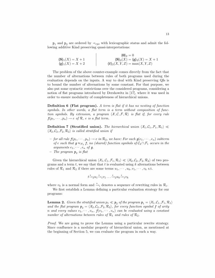
Example 4. Consider the following respective programs p1 (on the left) and p2:
g(t) → S(S(t)) f(S(x),0, t) → f(x, t, t)f(x,S(z), t) → f(x, z, g(t))
f(0,0, t) → t
Their hierarchical union p1 � p2 computes an exponential function. Using thenotation n for S(. . .S(0) . . .)︸ ︷︷ ︸
n times S
, we have JfK(n,m, p) = 3n × (2×m + p).
13
p1 and p2 are ordered by ≺rpo with lexicographic status and admit the fol-lowing additive Kind preserving quasi-interpretations:
L0M2 = 0LSM1(X) = X + 1 LSM2(X) = LgM2(X) = X + 1LgM1(X) = X + 2 LfM2(X, Y, Z) = max(X, Y, Z)
The problem of the above counter-example comes directly from the fact thatthe number of alternations between rules of both programs used during theevaluation depends on the inputs. A way to deal with Kind preserving QIs isto bound the number of alternations by some constant. For that purpose, wealso put some syntactic restrictions over the considered programs, considering anotion of flat programs introduced by Dershowitz in [17], where it was used inorder to ensure modularity of completeness of hierarchical unions.
Definition 6 (Flat program). A term is flat if it has no nesting of functionsymbols. In other words, a flat term is a term without composition of func-tion symbols. By extension, a program 〈X , C,F ,R〉 is flat if, for every rulef(p1, · · · , pn) → e of R, e is a flat term.
Definition 7 (Stratified union). The hierarchical union 〈X1, C1,F1,R1〉 �〈X2, C2,F2,R2〉 is called stratified union if
– for all rule f(p1, · · · , pn) → e in R2, we have: For each g(e1, · · · , en) subtermof e such that g ≈F2 f, no (shared) function symbols of C2∩F1 occurs in thearguments e1, · · · , en of g.
– The program p2 is flat
Given the hierarchical union 〈X1, C1,F1,R1〉 � 〈X2, C2,F2,R2〉 of two pro-grams and a term t, we say that that t is evaluated using k alternations betweenrules of R1 and R2 if there are some terms u1, · · · , uk, v1, · · · , vk s.t.
t∗→2u1
∗→1v1 . . .∗→2uk
∗→1vk
where vk is a normal form and ∗→i denotes a sequence of rewriting rules in Ri.We first establish a Lemma defining a particular evaluation strategy for our
programs:
Lemma 2. Given the stratified union p1 � p2 of the program p1 = 〈X1, C1,F1,R1〉and the flat program p2 = 〈X2, C2,F2,R2〉, for every function symbol f of arityn and every values v1, · · · , vn, f(v1, · · · , vn) can be evaluated using a constantnumber of alternations between rules of R1 and rules of R2.
Proof. We are going to prove the Lemma using a particular rewrite strategy.Since confluence is a modular property of hierarchical union, as mentioned atthe beginning of Section 5, we can evaluate the program in such a way.

14
First, we define a rank function from function symbols F to natural numbersN which satisfies
rkF (f) = 0 if 6 ∃g ∈ F , s.t. f >F g
rkF (f) = max(rkF (g)) + 1 if ∀g ∈ F s.t. f >F g
rkF (f) = rkF (g) if f ≈F g
The proof is by induction on the rank rkF2 :
– If f ∈ F1 then the result is obvious and without alternation.– Now suppose that f ∈ F2, we are going to show by induction that a function
symbol f in F2 of rank k can be evaluated using at most k + 1 alternations:– If rkF2(f) = 0 then every function symbol g appearing in the right handside of a rule defining the function symbol f is an equivalent fonction symbolfor the precedence ≥F2 . Consequently, by definition of stratified union, theevaluation of f can be performed, using only rules of R2. We first evaluateall these recursive calls. At the end either an error occurs or we obtain avalue in T (C1 ∪ C2). Now, since there are no longer function symbols in F2,we finish the evaluation with the function symbols of F1, applying only rulesin R1. Finally, we have performed the evaluation using only one alternation.– Now suppose that for rkF2(g) ≤ n, the evaluation of g(u1, · · · , uk) canbe performed using at most n + 1 alternations and take f s.t. rkF2(f) =n + 1. Since we consider a stratified union, every recursive call of the shapeh(v1, · · · , vm) with v1, · · · , vm values and h ≈F2 f can be performed usingonly rules in R2. The flat condition ensures that function symbols of F2
are not composed in the recursive calls. Indeed a recursive composition offunction symbols in F2 can lead to an unbounded number of alternations.Consequently, we can evaluate every recursive call of a function symbol h s.t.h ≈F2 f using only rules in R2. Now it remains to evaluate the function sym-bols of rank strictly smaller than n + 1. For that purpose, we evaluate theirarguments first. Since the program is flat, this evaluation is done using onlyrules of R1, so that we have a first alternation. Now we apply the inductionhypothesis, adding n + 1 more alternations, evaluating all these symbols inparallel which is possible since there is no composition, and eliminating allthe remaining function symbols in F2. It only remains function symbols inF1 that we evaluate using only rules in R1. Notice that this last evaluationdoes not add any alternation. Finally, we have evaluated a function symbolof rank n + 1 using at most n + 2 alternations of the rules in p1 and p2.
It remains to see that the rank of a function symbol is bounded by the size ofthe program and we obtain the required result. ut
Definition 8 (Extension). Given the hierarchical union of two programs p1
and p2 having respective QIs L−M1 and L−M2, define the extensions of the quasi-interpretation L−M1 (resp. L−M2), that we also note L−M1 (resp. L−M2), by thefollowing rules ∀b ∈ C2 ∪ F2\(C1 ∪ F1) (resp. C1 ∪ F1\(C2 ∪ F2)) LbM1 =def LbM2(resp. LbM2 =def LbM1).

15
The extensions of LM1 and LM2 are defined over all terms of p1 � p2. Noticethat these extensions preserve the fact that L−M1 and L−M2 are Kind preservingQIs.
Lemma 3. Given the hierarchical union of two programs p1 � p2 having Kindpreserving QIs L−M1 and L−M2, then there exist two polynomials P and Q s.t. forevery term w of p1 � p2, the extensions of L−M1 and L−M2 satisfy:
– LwM1 ≤ P (LwM2)– LwM2 ≤ Q(LwM1)
Proof. We exhibit the polynomial P , the result follows by symmetry of theKind preserving condition for the extensions of L−M1 and L−M2. Define α to bethe smallest multiplicative coefficient strictly greater than 1 of the polynomialsLbM2 (if there is no such a coefficient, then Definition 5 implies that the quasi-interpretations are similar, as in previous section) and β to be the greatestmultiplicative and additive coefficient of the polynomials LbM1, for every symbolb in T (C1 ∪ C2,F1 ∪ F2,X1 ∪ X2). Now we define four new assignments L−Mα,L−Mα=1, L−Mβ and L−Mβ=1:
– L−Mα is defined from L−M2 by replacing every multiplicative coefficient dis-tinct from 1 by α and every additive coefficient by 1.
– L−Mα=1 is defined from L−Mα by replacing every multiplicative coefficientdistinct from 1 by 1.
– L−Mβ is defined from L−M1 by replacing every multiplicative and additivecoefficient distinct from 1 by β.
– L−Mβ=1 is defined from L−Mβ by replacing every multiplicative and additivecoefficient distinct from 1 by 1.
Intuitively, L−Mα and L−Mβ represent respectively a lower bound on L−M2 and anupper bound on L−M1. We can show by structural induction that for any groundterm w, we have:
LwMα ≤ LwM2 By Definition of L−Mα (1)LwM1 ≤ LwMβ By Definition of L−Mβ (2)
LwMβ=1 = LwMα=1 By Condition 2 of Definition 5 (3)
Now, consider α (repsectively β) as a variable. LwMα (resp. LwMβ) can be seen asa polynomial in α (resp. β) (Even if the degree of the polynomial can dependon the size of the term w). Now suppose that LwMβ is a polynomial of degreed in β. Since β ≥ 1 by definition of QI, for every k ≤ d, βk ≤ βd. Write

16
LwMβ =∑d
i=1 γiβi, for some constants γi. We have:
LwMβ =d∑
i=1
γiβi (4)
≤ (d∑
i=1
γi)× βd Since β ≥ 1 (5)
= LwMβ=1 × βd By Definition of L−Mβ=1 (6)
= LwMα=1 × βd By Inequality (3) (7)
Define p to be the highest degree of the polynomials LbM1 and e be the degreeof LwMα in α. We are going to show by induction on the structure of the term wthat e ,d and p are linked throught the following inequality d ≤ p× e + 1:
– if w is a constant symbol (i.e. of arity 0), LwMα = LwMβ = 0. Consequently,d = e = 0 and the inequality is satisfied.
– Now suppose that w = h(t1, · · · , tn) with dj the degree of LtjMβ , and ej thedegree of LtjMα. By induction hypothesis, we have dj ≤ p×ej+1. Now supposethat LhMβ(X1, · · · , Xn) =
∑j1≤d1...jn≤dn
β × Xj11 ...Xjn
n . Let (i1, · · · , in) bethe the indices in the polynomial LhMβ where the degree d =
∑nj=1 djij + 1
is reached.
d ≤n∑
j=1
(p× ej + 1)ij + 1 = pn∑
j=1
ej × ij +n∑
j=1
ij + 1 By I.H.
≤ pn∑
j=1
ej × ij + p + 1 = p× (n∑
j=1
ej × ij + 1) + 1 By definition of p
≤ p× e + 1 By definition of e
Taking this result into account in inequality (7), we obtain:
LwMβ ≤ LwMα=1 × βp×e+1 = LwMα=1 × β(βp)e (8)
We take z such that αz ≥ βp and define the polynomial P by P (X) =β × Xz+1. Notice that such a z exists since α > 1 and that the polynomial Pdoes not depend on the term w but depends on the coefficients of the QIs.
It remains to check that LwM1 ≤ P (LwM2):
LwM1 ≤ LwMα=1 × β(βp)e By (8)≤ LwMα × β(βp)e Since α > 1≤ LwMα × β(αz)e = LwMα × β(αe)z By definition of z
≤ LwMα × β(LwMα)z) = P (LwMα) Since αe ≤ LwMα
≤ P (LwM2) By (1)
ut

17
Proposition 8. Given the stratified union p1 � p2 of two programs p1 =〈X1, C1,F1,R1〉 and p2 = 〈X2, C2,F2,R2〉 having additive Kind preserving quasi-interpretations L−M1 and L−M2, then, the Fundamental Lemma holds:
There is a polynomial P such that for any term t of p1 � p2 which has nvariables x1, · · · , xn, and for any ground substitution σ such that xiσ = vi:
|JtσK| ≤ P |t|( maxi=1..n
|vi|)
Proof. The proof is by structural induction on a term t.
(i) Consider the base case where t = f(x1, . . . , xk) for some variables xi. We usethe strategy of evaluation described in Lemma 2. So, the term is computedwithin ` alternation: f(v1, · · · , vn) = w0
∗→2u1∗→1w1 . . .
∗→2ul∗→1w`, with `
bounded by the rank.We are going to show by iduction on m ≤ l that there is a polynomial Rsuch that LwmM1 ≤ Rm(P (Lw0M2)) (I.H.).The base case m = 0 is trivial. Define R = Q ◦ P with P and Q the polyno-mials of Lemma 3. We have:
Lwm+1M2 ≤ Q(Lwm+1M1) By Lemma 3≤ Q(Lum+1M1) Proposition 1≤ Q(P (Lum+1M2)) By Lemma 3≤ Q(P (LwmM2)) Proposition 1≤ R(Rm(P (Lw0M2))) By I.H.
= Rm+1(P (Lw0M2))
Applying Fundamental Lemma to p2, we get a polynomial S. Then, Lw0M2 ≤S(maxi=1..n |vi|).So,
|w`| ≤ Lw`M2 ≤ R`(P (S( maxi=1..n
|vi|)))
We conclude taking P (X) = R` ◦ P ◦ S.(ii) The induction steps follows by composition of the polynomials.
And we obtain the required result. ut
Example 5. Consider the following programs p1 and p2:
d(S(x)) → S(S(d(x))) sq(S(x)) → S(add(sq(x), d(x)))d(0) → 0 sq(0) → 0
−−−−−− −−−−−−−add(S(x), y) → S(add(x, y))
add(0, y) → y
Their hierarchical union p1 � p2 = 〈X , C,F ,R〉 computes the square of a unarynumber given as input. For the precedence ≥F ,we have sq >F {add, d}. More-over the program p2 is flat since there is no composition of function symbols

18
in its rules. Consequently, p1 � p2 is a stratified union, since the argument ofthe recursive call sq(x) is a variable. Both p1 and p2 are ordered by ≺rpo withproduct status. Define the following quasi-interpretations L−M1 and L−M2 by:
L0M1 = 0 L0M2 = 0LSM1(X) = X + 1 LSM2(X) = X + 1LdM1(X) = 3×X LdM2(X) = 2×X
LaddM1(X, Y ) = X + Y LaddM2(X, Y ) = X + Y + 1LsqM2(X) = 2×X2
L−M1 and L−M2 are additive Kind preserving QIs, so that the program p1 � p2
computes values whose size is polynomially bounded by the inputs size. (BothQI of d illustrate the fact that they can be equal up to a multiplivative constantif the coefficient is > 1.)
Moreover the program division can be iterated on p1 by separating the rulesfor function symbols add and d, thus obtaining a constructor-sharing union.
Theorem 4 (time and space for hierarchical union of Kind preservingQIs). The set of functions computed by a hierarchical union of two programs p1
and p2 such that
1. p1 � p2 is a stratified union,2. p1 and p2 admit the respective additive Kind preserving QIs L−M1 and L−M2,3. p1 and p2 are ordered by ≺rpo and each function symbol has a product status,
is exactly the set of functions computable in polynomial time.Moreover, if condition (3) is replaced by: p1 and p2 are ordered by ≺rpo then
we characterize exactly the class of polynomial space functions.
Proof. Again, this result is a consequence of the fact that we have the Funda-mental Lemma in Proposition 8 and the ≺rpo ordering with product status, stillusing a call-by-value with cache. ut
6 Application to higher-order programs
Resource control of higher-order programs by QI is not straight forward, becausewe should deal at first glance with higher-order assignments. However, higher-order mechanisms can be reduced to an equivalent first order functional programby defunctionalization, which was introduced by Reynolds [37]. Defunctionaliza-tion consists in two steps. First, a new constructor symbol is substituted to everyhigher-order function declaration. Second, each function application is eliminatedby introducing a new function symbol for application. We refer to [15] which in-vestigates works related to Defunctionalization and Continuation-Passing Styleand gives a lot of references. Other higher-order removal techniques are treated,among others, by Wadler [40], Goguen [19] and Chin and Darlington [11].
This part is an application to modular approach to get QI as it is describedin the previous Section. So, we are not formalizing higher-order programs butwe rather illustrate the key concepts

19
Example 6. Suppose that g is defined by a program q3. Consider the followinghigher-order program p.
fold(λx.f(x),nil) → 0
fold(λx.f(x), c(x, l)) → f(fold(λx.f(x), l))h(l) → fold(λx.g(x), l) for g dfn in q3
h(l) iterates g such that JhK(l) = JgKn(0) where n is the number of elements inthe list l. From p, we obtain p by defunctionalization:
q1 =
ˆfold(nil) → 0
ˆfold(c(x, l)) → app(c0, ˆfold(l)) c0 is a new constructor
h(l) → ˆfold(l)
q2 ={app(c0, x) → g(x)
We are now able to use QI to higher-order programs by considering theirfirst-order transformations.Theorem 5 (time and space for higher-order programs).
– The set of functions computed by a higher-order program p such that thedefunctionalization p of p admits an additive quasi-interpretation and is or-dered by ≺rpo in which each function symbol has a product status is exactlythe set of functions computable in polynomial time.
– The set of functions computed by a higher-order program p such that thedefunctionalization p of p admits an additive quasi-interpretation and is or-dered by ≺rpo is exactly the set of functions computable in polynomial space.
In fact, the above example illustrates the fact that a defunctionalized programp is divided into three parts: the programs q1 and q2 above and a program q3
which computes g. Notice that the hierarchical union of q2 � q1 is stratified.Moreover they admit the following additive Kind preserving QIs:
L ˆfoldM1(X) = LhM1(X) = X LgM2(X) = X + 1LcM1(X, Y ) = X + Y + 1 Lc0M2 = 0
L0M1 = Lc0M1 = LnilM1 = 0 LappM2(X, Y ) = X + Y + 1LappM1(X, Y ) = X + Y + 1
Now, the results on modularity that we have previously established, allow us togive a sufficient condition on the QI of g defined in q3, in order to guarantee thatthe computation remains polynomially bounded. Indeed, Proposition 8 impliesthat LgM3 should be Kind preserving. That is, LgM3(X) = LgM2(X)+α = X+α+1,where α is some constant. Notice that LgM2 is forced by LappM2, and on the otherhand LappM2 is forced by LappM1.
Example 7. Consider the following program p, which visits a list l in continuationpassing style.
visit(nil, λx.f(x), y) → f(y)visit(c(x, l), λx.f(x), y) → visit(l, λx.g1(f(x)), y)
h(l) → visit(l, λx.g0(x), 0)

20
where g0 and g1 are defined by some program q3 which admits a additive QIL M3. We have JhK(l) = Jg1K
n(Jg0K(0)) where n is the number of elements in thelist l. We obtain p
q1 =
ˆvisit(nil, k, y) → app(k, y)
ˆvisit(c(x, l), k, y) → ˆvisit(l, c1(k), y)
h(l) → ˆvisit(l, c0, 0) c0 and c1 are new const.
q2 =
{app(c0, x) → g0(x)
app(c1(k), x) → g1(app(k, x))
The hierarchical union q2 � q1 is stratified and admit the following additiveKind preserving QIs:
L ˆvisitM1(X) = LhM1(X) = X + 1 Lg1M2(X) = Lg0M2(X) = X + 1Lc1M1(X, Y ) = LcM1(X, Y ) = X + Y + 1 Lc1M2(X) = X + 1
L0M1 = Lc0M1 = LnilM1 = 0 L0M2 = Lc0M2 = 0LappM1(X, Y ) = X + Y + 1 LappM2(X, Y ) = X + Y + 1
Now, suppose that we have two QI Lg0M3 and Lg1M3, which are two resourcecertificates for g0 and g1 wrt q3. Proposition 8 states that we are sure to remainpolynomial if the QI of g0 and g1 are kind preserving. In other words, Lg0M3(X) =X + α and Lg1M3(X) = X + β for some constants α and β.
So, a modular approach is a way to predict safely and efficiently if we can applya function in an higher-order computational mechanisms.
Finally, we state the following characterizations:
Theorem 6 (Modularity and higher-order programs). The set of func-tions computed by a higher-order programs p such that the defunctionalization p
is defined by hierarchical union p1 � p2 of two programs p1 and p2 satisfying:
1. p1 � p2 is a stratified union,2. p1 and p2 admit the respective additive Kind preserving QIs L−M1 and L−M2,3. p1 and p2 are ordered by ≺rpo and each function symbol has a product status,
is exactly the set of functions computable in polynomial time.Moreover, if condition (3) is replaced by: p1 and p2 are ordered by ≺rpo then
we characterize exactly the class of polynomial space functions.
7 Conclusion
One goal of this paper was to solve the problem of resource certificates, whenthey come attached to some programs. The question is how to recombine thosecertificates when programs are loaded. So we provide sufficient conditions fromwhich a resource bound is guaranteed. In particular, we have shown that this ap-proach was relevant for defunctionalized higher-order programs. We think that
21
another interesting direction is to consider mobile code in a functional program-ming setting, which could be a fragment of Boudol’s ULM [10].
Acknowledgments. The authors would like to thank C. Kirchner, for in-troducing the issue of Modularity and O. Danvy, for giving helpful comments onDefunctionalization, and the support of CRISS project.
References
1. R. Amadio. Max-plus quasi-interpretations. In Martin Hofmann, editor, TypedLambda Calculi and Applications, 6th International Conference, TLCA 2003, Va-lencia, Spain, June 10-12, 2003, Proceedings, volume 2701 of Lecture Notes inComputer Science, pages 31–45. Springer, 2003.
2. R. Amadio, S. Coupet-Grimal, S. Dal-Zilio, and L. Jakubiec. A functional scenariofor bytecode verification of resource bounds. In Jerzy Marcinkowski and AndrzejTarlecki, editors, Computer Science Logic, 18th International Workshop, CSL 13thAnnual Conference of the EACSL, Karpacz, Poland, volume 3210 of Lecture Notesin Computer Science, pages 265–279. Springer, 2004.
3. R. Amadio and S. Dal-Zilio. Resource control for synchronous cooperative threads.In Concur, pages 68–82, 2004.
4. D. Aspinall and A. Compagnoni. Heap Bounded Assembly Language. Journal ofAutomated Reasoning (Special Issue on Proof-Carrying Code), 31:261–302, 2003.
5. P. Baillot and K. Terui. A feasible algorithm for typing in elementary affine logic.In Springer, editor, TLCA, volume 3461 of Lecture Notes in Computer Science,pages 55–70, 2005.
6. G. Bonfante, J.-Y. Marion, and J.-Y. Moyen. On lexicographic termination or-dering with space bound certifications. In PSI 2001, Akademgorodok, Novosibirsk,Russia, Ershov Memorial Conference, volume 2244 of Lecture Notes in ComputerScience. Springer, Jul 2001.
7. G. Bonfante, J.-Y. Marion, and J.-Y. Moyen. Quasi-interpretation a way to controlresources. Submitted to Theoretical Computer Science, 2005. http://www.loria.
fr/~marionjy.
8. G. Bonfante, J.-Y. Marion, and J.-Y. Moyen. Quasi-interpretations and smallspace bounds. In Jurgen Giesl, editor, Term Rewriting and Applications, 16thInternational Conference, RTA 2005, Nara, Japan, April 19-21, 2005, Proceedings,volume 3467 of Lecture Notes in Computer Science, pages 150–164. Springer, 2005.
9. G. Bonfante, J.-Y. Marion, J.-Y. Moyen, and R. Pechoux. Synthesis of quasi-interpretations. Workshop on Logic and Complexity in Computer Science,LCC2005, Chicago, 2005. http://www.loria/~pechoux.
10. G. Boudol. Ulm, a core programming model for global computing. In ESOPconference, number 2986 in Lecture Notes in Computer Science, pages 234–248,2004.
11. W. N. Chin and J. Darlington. A higher-order removal method. Lisp Symb.Comput., 9(4):287–322, 1996.
12. S. Cook. Characterizations of pushdown machines in terms of time-bounded com-puters. Journal of the ACM, 18(1):4–18, January 1971.
13. P. Coppola and S. Ronchi Della Rocca. Principal typing for lambda calculus inelementary affine logic. Fundamenta Informaticae, 65(1-2):87–112, 2005.

22
14. S. Dal-Zilio and R. Gascon. Resource bound certification for a tail-recursive virtualmachine. In APLAS 2005 – 3rd Asian Symposium on Programming Languagesand Systems, volume 3780 of Lecture Notes in Computer Science, pages 247–263.Springer-Verlag, November 2005.
15. O. Danvy. An analytical approach to programs as data objects, 2006. Doctor Sci-entarum degree in Computer Science. BRICS. Departement of Computer Science.University of Aarhus.
16. N. Dershowitz. Orderings for term-rewriting systems. Theoretical Computer Sci-ence, 17(3):279–301, 1982.
17. N. Dershowitz. Hierachical termination. conditional and typed rewriting systems,4th international workshop, ctrs-94, jerusalem, israel, july 13-15, 1994, proceedings.In CTRS, volume 968 of Lecture Notes in Computer Science. Springer, 1995.
18. J.-Y. Girard. Light linear logic. Information and Computation, 143(2):175–204,1998. prsent a LCC’94, LNCS 960.
19. J. A. Goguen. Higher-order functions considered unnecessary for higher-order pro-gramming. In D. A. Turner, editor, Research Topics in Functional Programming,pages 309–351. Addison-Welsey, 1990.
20. B. Gramlich. Generalized sufficient conditions for modular termination of rewrit-ing. In In Proceedings of the Third International Conference on Algebraic andLogic Programming, volume 632, pages 53–68. Berlin: Springer Verlag, 1992.
21. M. Hofmann. A type system for bounded space and functional in-place update.Nordic Journal of Computing, 7(4):258–289, 2000.
22. M. Hofmann. The strength of Non-Size Increasing computation. In Proceedings ofPOPL’02, pages 260–269, 2002.
23. G. Huet. Confluent reductions: Abstract properties and applications to term rewrit-ing systems. Journal of the ACM, 27(4):797–821, 1980.
24. N. D. Jones. Computability and complexity, from a programming perspective. MITpress, 1997.
25. S. Kamin and J-J Levy. Attempts for generalising the recursive path orderings.Technical report, Univerity of Illinois, Urbana, 1980. Unpublished note. Accessibleon http://perso.ens-lyon.fr/pierre.lescanne/not accessible.html.
26. J.W. Klop. Term rewriting systems. In D. Gabbay S. Abramsky and T. Maibaum,editors, Handbook of logic in Computer Science, volume 2, pages 1–116. OxfordUniversity Press, 1992.
27. M. Kurihara and A. Ohuchi. Modularity of simple termination of term rewritingsystems with shared constructors. Theoretical Computer Science, 103:273–282,1992.
28. Y. Lafont. Soft linear logic and polynomial time. Theoretical Computer Science,318:163–180, 2004.
29. J.-Y. Marion. Analysing the implicit complexity of programs. Information andComputation, 183:2–18, 2003.
30. J.-Y. Marion and J.-Y. Moyen. Efficient first order functional program interpreterwith time bound certifications. In Michel Parigot and Andrei Voronkov, editors,Logic for Programming and Automated Reasoning, 7th International Conference,LPAR 2000, Reunion Island, France, volume 1955 of Lecture Notes in ComputerScience, pages 25–42. Springer, Nov 2000.
31. J.-Y. Marion and J.-Y. Moyen. Heap analysis for assembly programs. Technicalreport, Loria, 2006.
32. J.-Y. Marion and R. Pechoux. Resource analysis by sup-interpretation. InM. Hagiya and P. Wadler, editors, Functional and Logic Programming: 8th In-

23
ternational Symposium, FLOPS 2006, volume 3945 of Lecture Notes in ComputerScience, pages 163–176, 2006.
33. A. Middeldorp. Modular properties of term rewriting Systems. PhD thesis, VrijeUniversiteit te Amsterdam, 1990.
34. J.-Y. Moyen. Analyse de la complexite et transformation de programmes. Thesed’universite, Nancy 2, Dec 2003.
35. K.-H. Niggl and H. Wunderlich. Certifying polynomial time and linear/polynomialspace for imperative programs. SIAM Journal on Computing. to appear.
36. M.R.K. Krishna Rao. Modular proofs of completeness of hierarchical term rewrit-ing systems. Theoretical Computer Science, 151:487–512, 1995.
37. J. C. Reynolds. Definitional interpreters for higher-order programming languages.In ACM ’72: Proceedings of the ACM annual conference, pages 717–740. ACMPress, 1972.
38. Y. Toyama. Counterexamples for the direct sum of term rewriting systems. Infor-mation Processing Letters, 25:141–143, 1987.
39. Y. Toyama. On the church-rosser property for the direct sum of term rewritingsystems. Journal of the ACM, 34(1):128–143, 1987.
40. P. Wadler. Deforestation: Transforming programs to eliminate trees. In ESOP’88. European Symposium on Programming, Nancy, France, 1988 (Lecture Notesin Computer Science, vol. 300), pages 344–358. Berlin: Springer-Verlag, 1988.