Quasi-isometries of rank one S-arithmeticlattices

Kevin Wortman∗

December 7, 2007

Abstract

We complete the quasi-isometric classification of irreducible lat-tices in semisimple Lie groups over nondiscrete locally compact fieldsof characteristic zero by showing that any quasi-isometry of a rankone S-arithmetic lattice in a semisimple Lie group over nondiscretelocally compact fields of characteristic zero is a finite distance in thesup-norm from a commensurator.

1 Introduction

Throughout we let K be an algebraic number field, VK the set of all inequiv-alent valuations on K, and V ∞K ⊆ VK the subset of archimedean valuations.We will use S to denote a finite subset of VK that contains V ∞K , and we writethe corresponding ring of S-integers in K as OS. In this paper, G will alwaysbe a connected non-commutative absolutely simple algebraic K-group.

1.1 Commensurators

For any valuation v ∈ VK , we let Kv be the completion of K with respect tov. For any set of valuations S ′ ⊆ VK , we define

GS′ =∏v∈S′

G(Kv)

∗Supported in part by an N.S.F. Postdoctoral Fellowship.

1

and we identify G(OS) as a discrete subgroup of GS using the diagonalembedding.

We let Aut(GS) be the group of topological group automorphisms of GS.An automorphism ψ ∈ Aut(GS) commensurates G(OS) if ψ(G(OS))∩G(OS)is a finite index subgroup of both ψ(G(OS)) and G(OS).

We define the commensurator group of G(OS) to be the subgroup ofAut(GS) consisting of automorphisms that commensurate G(OS). Thisgroup is denoted as CommAut(GS)(G(OS)). Notice that it differs from thestandard definition of the commensurator group of G(OS) in that we havenot restricted ourselves to inner automorphisms.

1.2 Quasi-isometries

For constants L ≥ 1 and C ≥ 0, an (L,C) quasi-isometric embedding of ametric space X into a metric space Y is a function φ : X → Y such that forany x1, x2 ∈ X:

1

Ld(x1, x2

)− C ≤ d

(φ(x1), φ(x2)

)≤ Ld

(x1, x2

)+ C

We call φ an (L,C) quasi-isometry if φ is an (L,C) quasi-isometric em-bedding and there is a number D ≥ 0 such that every point in Y is withindistance D of some point in the image of X.

1.3 Quasi-isometry groups

For a metric space X, we define the relation ∼ on the set of functions X → Xby φ ∼ ψ if

supx∈X

d(φ(x), ψ(x)

)<∞

In this paper we will call two functions equivalent if they are related by ∼.For a finitely generated group with a word metric Γ, we form the set of all

quasi-isometries of Γ, and denote the quotient space modulo ∼ byQI(Γ). Wecall QI(Γ) the quasi-isometry group of Γ as it has a natural group structurearising from function composition.

1.4 Main result

In this paper we show:

2

Theorem 1.4.1. Suppose K is an algebraic number field, G is a connectednon-commutative absolutely simple algebraic K-group, S properly containsV ∞K , and rankK(G) = 1. Then there is an isomorphism

QI(G(OS)) ∼= CommAut(GS)(G(OS))

Two special cases of Theorem 1.4.1 had been previously known: Tabackproved it when G(OS) is commensurable to PGL2(Z[1/p]) where p is a primenumber [Ta] (we’ll use Taback’s theorem in our proof), and it was provedwhen rankKv(G) ≥ 2 for all v ∈ S by the author in [Wo 1].

Examples of S-arithmetic groups for which Theorem 1.4.1 had been pre-viously unknown include when G(OS) = PGL2(Z[1/m]) where m is com-posite. Theorem 1.4.1 in this case alone was an object of study; see Taback-Whyte [Ta-Wh] for their program of study. Theorem 2.4.1 below presents ashort proof of this case.

1.5 Quasi-isometry groups of non-cocompact irreducibleS-arithmetic lattices

Combining Theorem 1.4.1 with the results from Schwartz, Farb-Schwartz,Eskin, Farb, Taback, and Wortman ([Sch 1], [Fa-Sch], [Sch 2], [Es], [Fa],[Ta], and [Wo 1]) we have

Theorem 1.5.1. Suppose K is an algebraic number field, and G is a con-nected, non-commutative, absolutely simple, K-isotropic, algebraic K-group.If either K Q, S 6= V ∞K , or G is not Q-isomorphic to PGL2, then thereis an isomorphism

QI(G(OS)) ∼= CommAut(GS)(G(OS))

Note that Theorem 1.5.1 identifies the quasi-isometry group of any non-cocompact irreducible S-arithmetic lattice in a semisimple Lie group overnondiscrete locally compact fields of characteristic 0 that is not virtuallyfree.

Indeed, the condition that G is K-isotropic is equivalent to G(OS) beingnon-cocompact, and it is well known that G(OS) is virtually free only whenK ∼= Q, S = V ∞K , and G is Q-isomorphic to PGL2. In this case, G(OS) iscommensurable with PGL2(Z).

3

1.6 Cocompact case

By Kleiner-Leeb [K-L], the classification of quasi-isometries of cocompact S-arithmetic lattices reduces to the classification of quasi-isometries of real andp-adic simple Lie groups. This classification is known; see e.g. [Fa] for anaccount of the cases not covered in [K-L].

1.7 Function fields

Our proof of Theorem 1.4.1 also applies when K is a global function fieldwhen we add the hypothesis that there exists v, w ∈ S such that rankKv(G) =1 and rankKw(G) ≥ 2.

For more on what is known about the quasi-isometry groups of arithmeticgroups over function fields – and for a conjectural picture of what is unknown– see [Wo 2].

1.8 Outline of the proof and the paper

We begin Section 2 with a sort of large-scale reduction theory. We examinea metric neighborhood, N , of an orbit of an S-arithmetic group, Γ, insidethe natural product of Euclidean buildings and symmetric spaces, X. InSection 2.2 we show that the fibers of N under projections to building factorsof X are geometric models for S-arithmetic subgroups of Γ.

In Section 2.3, we apply results from [Wo 1] to extend a quasi-isometryφ : Γ→ Γ to the space X that necessarily preserves factors.

Our general approach to proving Theorem 1.4.1 is to restrict φ to factorsofX and use the results from Section 2.2 to decompose φ into quasi-isometriesof S-arithmetic subgroups of Γ. Once each of these “sub-quasi-isometries”is understood, they are pieced together to show that φ is a commensurator.An easy example of this technique is given in Section 2.4 by PGL2(Z[1/m]).We then treat the general case of Theorem 1.4.1 in Section 2.5

Our proof in Section 2.5 relies on the structure of horoballs for S-arithmeticgroups associated to the product of a symmetric space and a single tree. Weprove the results that we need for these horoballs (that they are connected,pairwise disjoint, and reflect a kind of symmetry in factors) in Section 3, sothat Section 3 is somewhat of an appendix. The proof is organized in thisway because, in the author’s opinion, it just makes it easier to digest the ma-terial. There would be no harm though in reading Section 3 after Section 2.4

4

and before Section 2.5 for those who prefer a more linear presentation.

1.9 Acknowledgements

I was fortunate to have several conversations with Kevin Whyte on the con-tents of this paper, and am thankful for those. In particular, he brought tomy attention that SL2(Z) is the only non-cocompact arithmetic lattice inSL2(R) up to commesurability.

I am also grateful to the following mathematicians who contributed to thispaper: Tara Brendle, Kariane Calta, Indira Chatterji, Alex Eskin, BensonFarb, Dan Margalit, Dave Witte Morris, and Jennifer Taback.

2 Proof of Theorem 1.4.1

Let G, K, and S be as in Theorem 1.4.1, and let φ : G(OS)→ G(OS) be aquasi-isometry.

2.1 Geometric models

For each valuation v of K, we let Xv be the symmetric space or Euclideanbuilding corresponding to G(Kv). If S ′ is a finite set of valuations of K, welet

XS′ =∏v∈S′

Xv

Recall that there is a natural inclusion of topological groups Aut(GS′) →Isom(XS′).

Let O be the ring of integers in K, and fix a connected subspace ΩV∞K⊆

XV∞Kthat G(O) acts cocompactly on. Let D∞ ⊆ XV∞K

be a fundamentaldomain for this action.

For each nonarchimedean valuation w ∈ S − V ∞K , we denote the ring ofintegers in Kw by Ow. The group G(Ow) is bounded in G(Kw), so G(Ow)fixes a point xw ∈ Xw. We choose a bounded set Dw ⊆ Xw containing xwwith G(OS)Dw = Xw and such that gxw ∈ Dw for g ∈ G(OS) implies thatgxw = xw.

For any set of valuations S ′ satisfying V ∞K ⊆ S ′ ⊆ S, we define the space

ΩS′ = G(OS′)(D∞ ×

∏w∈S′−V∞K

Dw

)5

Note that ΩS′ is a subspace of XS′ .We endow ΩS′ with the path metric. Since G(OS′) acts cocompactly on

ΩS′ , we have the following observation:

Lemma 2.1.1. For V ∞K ⊆ S ′ ⊆ S, the space ΩS′ is quasi-isometric to thegroup G(OS′).

2.2 Fibers of projections to buildings are S-arithmetic

In the large-scale, the fibers of the projection of ΩS onto building factors ofXS are also S-arithmetic groups (or more precisely, S ′-arithmetic groups).This is the statement of Lemma 2.2.2 below, but we will start with a proofof a special case.

Lemma 2.2.1. The Hausdorff distance between

ΩS ∩(XS′ ×

∏w∈S−S′

xw)

andΩS′ ×

∏w∈S−S′

xw

is finite.

Proof. There are three main steps in this proof.First, if y ∈ ΩS′ , then y = gd for some g ∈ G(OS′) and some

d ∈ D∞ ×∏

w∈S′−V∞K

Dw

Since G(OS′) ≤ G(Ow) for all w ∈ S − S ′, it follows from our choice of thepoints xw that

y ×∏

w∈S−S′xw = g

(d ×

∏w∈S−S′

xw)⊆ ΩS

Therefore,

ΩS′ ×∏

w∈S−S′xw ⊆ ΩS ∩

(XS′ ×

∏w∈S−S′

xw)

(1)

6

Second, we suppose

y ×∏

w∈S−S′xw ⊆ ΩS

for some y ∈ XS′ . Then there exists a g ∈ G(OS) such that

gy ∈ D∞ ×∏

w∈S′−V∞K

Dw

and gxw ∈ Dw for all w ∈ S − S ′. Notice that our choice of Dw impliesgxw = xw for all w ∈ S − S ′. Thus, g is contained in the compact group

Hw = h ∈ G(Kw) | hxw = xw

for all w ∈ S − S ′. Consequently, g is contained in the discrete group

G(OS) ∩(GS′ ×

∏w∈S−S′

Hw

)We name this discrete group ΓS′ .

Note that we have shown

y ×∏

w∈S−S′xw ⊆ ΓS′

(D∞ ×

∏w∈S−V∞K

Dw

)Therefore,

ΩS ∩(XS′ ×

∏w∈S−S′

xw)⊆ ΓS′

(D∞ ×

∏w∈S−V∞K

Dw

)(2)

Third, we recall that

G(OS′) = G(OS) ∩(GS′ ×

∏w∈S−S′

G(Ow))

and use the definition of ΓS′ coupled with the fact that G(Ow) ≤ Hw tosee that ΓS′ contains G(OS′). Since, ΓS′ and G(OS′) are lattices in GS′ ×∏

w∈S−S′ Hw, the containment G(OS′) ≤ ΓS′ is of finite index. Therefore,the Hausdorff distance between

ΓS′(D∞ ×

∏w∈S′−V∞K

Dw ×∏

w∈S−S′xw

)7

and

ΩS′ ×∏

w∈S−S′xw = G(OS′)

(D∞ ×

∏w∈S′−V∞K

Dw ×∏

w∈S−S′xw

)is finite. Combined with (1) and (2) above, the lemma follows.

The more general form of Lemma 2.2.1 that we will use in our proof ofTheorem 1.4.1 is the following lemma. We will use the notation of xS−S′ forthe point (xw)w∈S−S′ ∈ XS−S′ .

Lemma 2.2.2. Suppose V ∞K ⊆ S ′ ⊆ S. If y ∈ XS−S′ and y ∈ G(OS)xS−S′,then the Hausdorff distance between

ΩS ∩(XS′ × y

)and

ΩS′ × yis finite.

Remark. Our assumption in Lemma 2.2.2 that y ∈ G(OS)xS−S′ is not aserious restriction over the assumption that y ∈ XS−S′ . Indeed, G(OS) isdense in GS−S′ , so the orbit G(OS)xS−S′ is a finite Hausdorff distance fromthe space XS−S′ .

Proof. Let g ∈ G(OS) be such that y = gxS−S′ . Then

h ∈ G(OS) | hxS−S′ = y = gh ∈ G(OS) | hxS−S′ = xS−S′

= g(G(OS) ∩

(GS′ ×

∏w∈S−S′

Hw

))= gΓS′

where Hw and ΓS′ are as in the proof of the previous lemma.Now by our choice of the points xw ∈ Xw for w ∈ S−V ∞K at the beginning

of this section, we have

ΩS ∩(XS′ × y

)= G(OS)

(D∞ ×

∏w∈S−V∞K

Dw

)∩(XS′ × y

)= gΓS′

(D∞ ×

∏w∈S′−V∞K

Dw

)× y

8

Notice that the final space from the above chain of equalities is a finiteHausdorff distance from

gG(OS′)(D∞ ×

∏w∈S′−V∞K

Dw

)× y

since ΓS′ is commensurable with G(OS′).Because g commensurates G(OS′), the above space is also a finite Haus-

dorff distance from ΩS′ × y.

2.3 Extending quasi-isometries of ΩS to XS

Applying Lemma 2.1.1, we can regard our quasi-isometry φ : G(OS) →G(OS) as a quasi-isometry of ΩS. Our goal is to show that φ is equivalentto an element of CommAut(GS)(G(OS)), and we begin by extending φ to aquasi-isometry of XS.

Lemma 2.3.1. There is a permutation of S, which we name τ , and thereare quasi-isometries

φv : Xv → Xτ(v)

such that the restriction of the quasi-isometry

φS =∏v∈S

φv : XS → XS

to ΩS is equivalent to φ. If Xv is a higher rank space for any v ∈ S, then φvmay be taken to be an isometry.

Proof. By Proposition 6.9 of [Wo 1], the quasi-isometry φ : ΩS → ΩS extendsto a quasi-isometry of X. That is there is some quasi-isometry φ : X → Xsuch that φ ∼ φ|ΩS where φ|ΩS is the restriction of φ to ΩS.

The map φ preserves factors in the boundary of X and an argument ofEskin’s – Proposition 10.1 of [Es] – can be directly applied to show thatφ is equivalent to a product of quasi-isometries of the factors of X, up topermutation of factors.

Note that the statement of Proposition 10.1 from [Es] claims that Xv andXτ(v) are isometric for v ∈ V ∞K . This is because quasi-isometric symmetricspaces are isometric up to scale.

9

2.4 Example of proof to come

Before continuing with the general proof, we’ll pause for a moment to demon-strate the utility of Lemmas 2.2.2 and 2.3.1 by proving the following specialcase of Theorem 1.4.1.

Theorem 2.4.1. If m ∈ N and m 6= 1, then

QI(PGL2(Z[1/m])

) ∼= PGL2(Q)

Proof. Let K = Q, G = PGL2, and S = v∞ ∪ vpp|m where v∞ isthe archimedean valuation and vp is the p-adic valuation. Thus, G(OS) =PGL2(Z[1/m]), the space Xv∞ is the hyperbolic plane, and Xvp is a (p+ 1)-valent regular tree.

If φ : PGL2(Z[1/m]) → PGL2(Z[1/m]) is a quasi-isometry, then byLemma 2.3.1 we can replace φ by a quasi-isometry φS which is the productof quasi-isometries

φ∞ : Xv∞ → Xv∞

andφp : Xvp → Xvτ(p)

for some permutation τ of the primes dividing m.If m is prime, then this theorem reduces to Taback’s theorem [Ta]. Now

suppose ` is a prime dividing m. We let S ′ = v∞ , v` and S ′′ = v∞ , vτ(`) .It follows from the density of PGL2(Z[1/m]) in∏

p|m ; p 6=τ(`)

PGL2(Qp)

that any point in XS−S′′ is a uniformly bounded distance from the orbitPGL2(Z[1/m])xS−S′′ . Therefore, we may assume that there is some y ∈PGL2(Z[1/m])xS−S′′ such that φS

(XS′ × xS−S′

)⊆ XS′′ × y.

Since φ(ΩS) ⊆ ΩS, we may assume that φS(ΩS ∩ (XS′ × xS−S′)

)⊆

ΩS ∩ (XS′′ × y). It follows from Lemma 2.2.2 that φS restricts to a quasi-isometry between ΩS′ × xS−S′ and ΩS′′ × y.

Note that by the product structure of φS, we can assume that φ∞ × φ`restricts to a quasi-isometry between ΩS′ and ΩS′′ — or by Lemma 2.1.1, aquasi-isometry between PGL2(Z[1/`]) and PGL2(Z[1/τ(`)]). Taback showedthat for any such quasi-isometry we must have ` = τ(`) and that φ∞ × φ` isequivalent to a commensurator g∞ × g` ∈ PGL2(R)×PGL2(Q`) where g∞

10

and g` must necessarily be included in, and represent the same element of,PGL2(Q) [Ta].

As the above paragraph is independent of the prime `|m, the elementg∞ ∈ PGL2(Q) determines φS and thus φ.

Having concluded our proof of the above special case, we return to thegeneral proof. Our goal is to show that φS is equivalent to an element ofCommAut(GS)(G(OS)). At this point, the proof breaks into two cases.

2.5 Case 1: GV∞Kis not locally isomorphic to PGL2(R)

Notice that CommAut(GS)(G(OS)) acts by isometries on XS. So a good firststep toward our goal is to show that φS is equivalent to an isometry. First,we will show that φV∞K is equivalent to an isometry.

Lemma 2.5.1. The quasi-isometry φV∞K : XV∞K→ XV∞K

is equivalent to anisometry of the symmetric space XV∞K

. Indeed, it is equivalent to an elementof CommAut(GS)(G(O)).

Proof. Notice that φV∞K is simply the restriction of φS to XV∞K× xS−V∞K .

Since G(OS) is dense inGS−V∞K , the Hausdorff distance between G(OS)xS−V∞KandXS−V∞K is finite. Thus, by replacing φS with an equivalent quasi-isometry,we may assume that XV∞K

×xS−V∞K is mapped by φS into a space XV∞K×y

for some y ∈ XS−V∞K with y ∈ G(OS)xS−V∞K .Since the Hausdorff distance between φS(ΩS) and ΩS is finite, we have

by Lemmas 2.2.2 and 2.1.1 that φV∞K induces a quasi-isometry of G(O). Thelemma follows from the existing quasi-isometric classification of arithmeticlattices using our assumption in this Case that GV∞K

is not locally isomorphicto PGL2(R); see [Fa].

At this point, it is not difficult to see that Theorem 1.4.1 holds in thecase when every nonarchimedean factor of GS is higher rank:

Lemma 2.5.2. If rankKv(G) ≥ 2 for all v ∈ S − V ∞K then φS is equivalentto an element of CommAut(GS)(G(OS)).

11

Proof. By Lemma 2.3.1, φv is equivalent to an isometry for all v ∈ S − V ∞K .Combined with Lemma 2.5.1, we know that φS is equivalent to an isometry.

That φS is equivalent to an element of CommAut(GS)(G(OS)) follows fromProposition 7.2 of [Wo 1]. Indeed, any isometry of XS that preserves ΩS upto finite Hausdorff distance corresponds in a natural way to an automorphismof GS that preserves G(OS) up to finite Hausdorff distance, and any suchautomorphism of GS is shown in Proposition 7.2 of [Wo 1] to be a commen-surator.

For the remainder of Case 1, we are left to assume that there is at leastone w ∈ S − V ∞K such that rankKw(G) = 1.

Before beginning the proof of the next and final lemma for Case 1, it willbe best to recall some standard facts about boundaries.

Tree boundaries. If w is a nonarchimedean valuation ofK, and rankKw(G) =1, then Xw is a tree.

For any minimal Kw-parabolic subgroup of G, say M, we let εM be theend of Xw such that M(Kw)εM = εM. Notice that the space of all ends ofthe form εP where P is a minimal K-parabolic subgroup of G forms a densesubset of the space of ends of Xw.

Tits boundaries. For any minimal K-parabolic subgroup of G, say P, welet δP be the simplex in the Tits boundary of XV∞K

corresponding to thegroup

∏v∈V∞K

P(Kv).

If δ is a simplex in the Tits boundary of XV∞K, and ε is an end of the tree

Xw, then we denote the join of δ and ε by δ ∗ ε. It is a simplex in the Titsboundary of XT where T = V ∞K ∪ w.

Lemma 2.5.3. Let w ∈ S − V ∞K be such that rankKw(G) = 1. Then φw :Xw → Xτ(w) is equivalent to an isometry that is induced by an isomorphismof topological groups G(Kw)→ G(Kτ(w)).

Proof. Below, we will denote the set of valuations V ∞K ∪ τ(w) by T τ .We begin by choosing a minimal K-parabolic subgroup of G, say P, and

a geodesic ray ρ : R≥0 → XT that limits to the interior of the simplex δP∗εP.By Lemma 2.5.1, the image of φT ρ under the projection XT → XV∞K

limits to a point in the interior of δQ for some minimal K-parabolic subgroupQ. Similarly, φw is a quasi-isometry of a tree, so it maps each geodesic

12

ray into a bounded neighborhood of a geodesic ray that is unique up tofinite Hausdorff distance. Thus, the image of φT ρ under the projectionXT → Xτ(w) limits to εQ′ for some minimal Kτ(w)-parabolic subgroup Q′.Together, these results imply that φT ρ is a finite Hausdorff distance froma geodesic ray that limits to a point in the interior of δQ ∗ εQ′ .

By Lemma 3.4.1, there is a subspaceHP of XT corresponding to P (calleda “T -horoball”) such that

t 7→ d(ρ(t) , XT −HP

)is an unbounded function. Thus,

t 7→ d(φT ρ(t) , XT τ − φT (HP)

)is also unbounded.

Using Lemma 3.2.1 and the fact that φT (ΩT ) is a finite Hausdorff distancefrom ΩT τ , we may replace φT with an equivalent quasi-isometry to deducethat φT (HP) is contained in the union of all T τ -horoballs in XT τ .

It will be clear from the definition given in Section 3 that each T -horoballis connected. In addition, Lemma 3.2.2 states that the collection of T τ -horoballs is pairwise disjoint, so it follows that φT (HP) is a finite distancefrom a single T τ -horoball HM ⊆ XT τ where M is a minimal K-parabolicsubgroup of G. Therefore,

t 7→ d(φT ρ(t) , XT τ −HM

)is unbounded.

Because the above holds for all ρ limiting to δP ∗ εP, and because φT ρlimits to δQ ∗ εQ′ , we have by Lemma 3.4.2, that Q = M = Q′. That is,φV∞K completely determines the map that φw induces between the ends of thetrees Xw and Xτ(w) that correspond to K-parabolic subgroups of G.

Recall that by Lemma 2.5.1, φV∞K is equivalent to a commensurator ofG(O) ≤ GV∞K

. Using Lemma 7.3 of [Wo 1], φV∞K (regarded as an automor-phism of GV∞K

) restricts to G(K) as a composition

δ σ : G(K)→ G(K)

13

where σ is an automorphism of K,

σ : G(K)→ σG(K)

is the map obtained by applying σ to the entries of elements in G(K), and

δ : σG→ G

is a K-isomorphism of K-groups.Thus, if ∂Xw and ∂Xτ(w) are the space of ends of the trees Xw and Xτ(w)

respectively, and if ∂φw : ∂Xw → ∂Xτ(w) is the boundary map induced byφw, then we have shown that

∂φw(εP) = εδ(σP)

for any P ≤ G that is a minimal K-parabolic subgroup of G.

Our next goal is to show that the valuation w σ−1 is equivalent to τ(w).If this is the case, then δ σ extends from a group automorphism of G(K)to a topological group isomorphism

αw : G(Kw)→ G(Kτ(w))

If ∂αw : ∂Xw → ∂Xτ(w) is the map induced by αw, then ∂αw equals ∂φwon the subset of ends in ∂Xw corresponding to K-parabolic subgroups of Gsince αw extends δ σ. Therefore, ∂αw = ∂φw on all of ∂Xw by the densityof the “K-rational ends” in ∂Xw. Thus, αw determines φw up to equivalence.This would prove our lemma.

So to finish the proof of this lemma, we will show that wσ−1 is equivalentto τ(w).

For any maximal K-split torus S ≤ G, we let γwS ⊆ Xw (resp. γτ(w)S ⊆

Xτ(w)) be the geodesic that S(Kw) (resp. S(Kτ(w))) acts on by translations.Fix S and T, two maximal K-split tori in G such that γwS∩γwT is nonempty

and bounded. We choose a point a ∈ γwS ∩ γwT.Since S(OT ) is dense in S(Kw), there exists a group element gn ∈ S(OT )

for each n ∈ N such that

d(gn(γwT) , a

)> n

14

Note that gn(γwT) = γwgnTg

−1n

. Thus

d(φw(γw

gnTg−1n

) , φw(a))

is an unbounded sequence.As gnTg

−1n is K-split, φw(γw

gnTg−1n

) is a uniformly bounded Hausdorff dis-

tance fromγτ(w)

δσ(gnTg−1n )

= δ σ(gn)γτ(w)δσ(T)

because a geodesic in Xτ(w) is determined by its two ends.We finally have that

d(δ σ(gn)γ

τ(w)δσ(T) , φw(a)

)is an unbounded sequence. It is this statement that we shall contradict byassuming that w σ−1 is inequivalent to τ(w).

Note that gn ∈ G(Ov) for all v ∈ VK − T since gn ∈ S(OT ). Thus,σ0(gn) ∈ σG(Ovσ−1) for all v ∈ VK − T . If it were the case that w σ−1

is inequivalent to τ(w), then it follows that σ0(gn) ∈ σG(Oτ(w)). Hence,δ σ0(gn) defines a bounded sequence in G(Kτ(w)). Therefore,

d(δ σ(gn)γ

τ(w)δσ(T) , φw(a)

)is a bounded sequence, our contradiction.

The proof of Theorem 1.4.1 in Case 1 is complete with the observationthat applications of Lemma 2.5.3 to tree factors, allows us to apply theProposition 7.2 of [Wo 1] as we did in Lemma 2.5.2.

2.6 Case 2: GV∞Kis locally isomorphic to PGL2(R)

It follows that V ∞K contains a single valuation v, and that Kv∼= R. Thus

K = Q, and V ∞K is the set containing only the standard real metric on Q.Our assumption that G is absolutely simple implies that GV∞K

is actuallyisomorphic to PGL2(R). Thus, G is a Q-form of PGL2. As we are assumingthat G is Q-isotropic, it follows from the classification of Q-forms of PGL2

that G and PGL2 are Q-isomorphic (see e.g. page 55 of [Ti]).

15

From our assumptions in the statement of Theorem 1.4.1, S 6= V ∞K . Asthe only valuations, up to scale, on Q are the real valuation and the p-adicvaluations, G(OS) is commensurable with PGL2(Z[1/m]) for some m ∈ Nwith m 6= 1. Thus, Case 2 of Theorem 1.4.1 follows from Theorem 2.4.1.

Our proof of Theorem 1.4.1 is complete modulo the material from Sec-tion 3.

3 Horoball patterns in a product of

a tree and a symmetric space

In this section we will study the components of XS−ΩS when XS is a productof a symmetric space and a tree.

Setting notation. We let w be a nonarchimedean valuation on K such thatrankKw(G) = 1. Then we set T equal to V ∞K ∪ w.

3.1 Horoballs in rank one symmetric spaces.

Let P be a minimal K-parabolic subgroup of G. As in the previous section,we let δP be the simplex in the Tits boundary of XV∞K

corresponding to thegroup

∏v∈V∞K

P(Kv).

Note that G being K-isotropic and rankKw(G) = 1 together implies thatrankK(G) = 1. Borel proved that the latter equality implies that XV∞K

−ΩV∞Kcan be taken to be a disjoint collection of horoballs (17.10 [Bo]).

To any horoball of XV∞K−ΩV∞K

, say H, there corresponds a unique δP asabove such that any geodesic ray ρ : R≥0 → XV∞K

that limits to δP definesan unbounded function

t 7→ d(ρ(t) , XV∞K

−H)

3.2 T -horoballs in XT

Let y ∈ Xw and suppose y ∈ G(OT )xw. Recall that by Lemma 2.2.2, thespace ΩT ∩

(XV∞K

× y)

is a finite Hausdorff distance from ΩV∞K× y.

For any minimal K-parabolic subgroup of G, say P, we let HyP,∞ ⊆

XV∞K× y be the horoball of ΩT ∩

(XV∞K

× y)

that corresponds to δP.

16

For arbitrary x ∈ Xw, we define

HxP,∞ = Hy

P,∞

where y ∈ G(OT )xw minimizes the distance between x and G(OT )xw.We let

HP =⋃x∈Xw

(Hx

P,∞ × x)

Each of the spaces HP is called a T -horoball.Let P be the set of all minimalK-parabolic subgroups of G. The following

lemma follows directly from our definitions. It will be used in the proof ofLemma 2.5.3.

Lemma 3.2.1. The Hausdorff distance between XT − ΩT and⋃P∈P

HP

is finite.

We record another observation to be used in the proof of Lemma 2.5.3.

Lemma 3.2.2. If P 6= Q are minimal K-parabolic subgroups of G, thenHP ∩HQ = ∅.

Proof. The horoballs comprising(XV∞K

−ΩV∞K

)×xw are pairwise disjoint,

and are a finite Hausdorff distance from the horoballs of ΩT ∩(XV∞K

×xw)

by Lemma 2.2.1. Hence, if y = gxw for some g ∈ G(OT ), then the horoballsdetermined by

ΩT ∩(XV∞K

× y)

= g[ΩT ∩

(XV∞K

× xw)]

are disjoint.

3.3 Deformations of horoballs over geodesics in Xw

We let π : XT → XV∞Kbe the projection map. Note that if x ∈ Xw and P is

a minimal K-parabolic subgroup of G, then π(HxP,∞) is a horoball in XV∞K

that is based at δP.Recall that for any minimal Kw-parabolic subgroup of G, say Q, we

denote the point in the boundary of the tree Xw that corresponds to Q(Kw)by εQ.

17

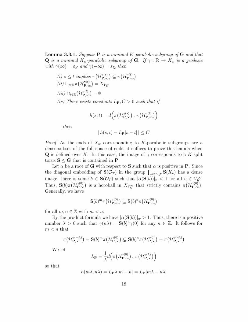
Lemma 3.3.1. Suppose P is a minimal K-parabolic subgroup of G and thatQ is a minimal Kw-parabolic subgroup of G. If γ : R → Xw is a geodesicwith γ(∞) = εP and γ(−∞) = εQ then

(i) s ≤ t implies π(Hγ(s)

P,∞)⊆ π

(Hγ(t)

P,∞)

(ii) ∪t∈Rπ(Hγ(t)

P,∞)

= XV∞K

(iii) ∩t∈R(Hγ(t)

P,∞)

= ∅(iv) There exists constants LP, C > 0 such that if

h(s, t) = d(π(Hγ(s)

P,∞), π(Hγ(t)

P,∞))

then|h(s, t)− LP|s− t| | ≤ C

Proof. As the ends of Xw corresponding to K-parabolic subgroups are adense subset of the full space of ends, it suffices to prove this lemma whenQ is defined over K. In this case, the image of γ corresponds to a K-splittorus S ≤ G that is contained in P.

Let α be a root of G with respect to S such that α is positive in P. Sincethe diagonal embedding of S(OT ) in the group

∏v∈V∞K

S(Kv) has a dense

image, there is some b ∈ S(OT ) such that |α(S(b))|v < 1 for all v ∈ V ∞K .

Thus, S(b)π(Hγ(0)

P,∞)

is a horoball in XV∞Kthat strictly contains π

(Hγ(0)

P,∞).

Generally, we have

S(b)mπ(Hγ(0)

P,∞)( S(b)nπ

(Hγ(0)

P,∞)

for all m,n ∈ Z with m < n.By the product formula we have |α(S(b))|w > 1. Thus, there is a positive

number λ > 0 such that γ(nλ) = S(b)nγ(0) for any n ∈ Z. It follows form < n that

π(Hγ(mλ)

P,∞)

= S(b)mπ(Hγ(0)

P,∞)( S(b)nπ

(Hγ(0)

P,∞)

= π(Hγ(nλ)

P,∞)

We let

LP =1

λd(π(Hγ(0)

P,∞), π(Hγ(λ)

P,∞))

so thath(mλ, nλ) = LPλ|m− n| = LP|mλ− nλ|

18

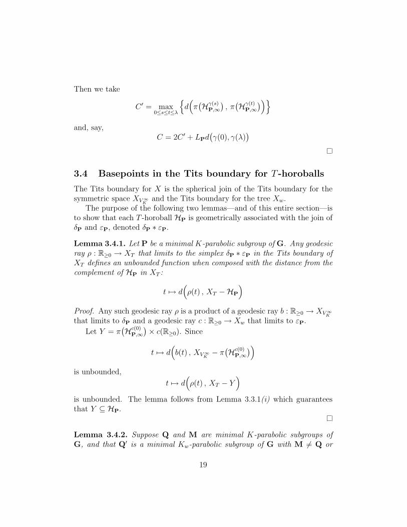
Then we take

C ′ = max0≤s≤t≤λ

d(π(Hγ(s)

P,∞), π(Hγ(t)

P,∞))

and, say,C = 2C ′ + LPd

(γ(0), γ(λ)

)

3.4 Basepoints in the Tits boundary for T -horoballs

The Tits boundary for X is the spherical join of the Tits boundary for thesymmetric space XV∞K

and the Tits boundary for the tree Xw.The purpose of the following two lemmas—and of this entire section—is

to show that each T -horoball HP is geometrically associated with the join ofδP and εP, denoted δP ∗ εP.

Lemma 3.4.1. Let P be a minimal K-parabolic subgroup of G. Any geodesicray ρ : R≥0 → XT that limits to the simplex δP ∗ εP in the Tits boundary ofXT defines an unbounded function when composed with the distance from thecomplement of HP in XT :

t 7→ d(ρ(t) , XT −HP

)Proof. Any such geodesic ray ρ is a product of a geodesic ray b : R≥0 → XV∞Kthat limits to δP and a geodesic ray c : R≥0 → Xw that limits to εP.

Let Y = π(Hc(0)

P,∞)× c(R≥0). Since

t 7→ d(b(t) , XV∞K

− π(Hc(0)

P,∞))

is unbounded,

t 7→ d(ρ(t) , XT − Y

)is unbounded. The lemma follows from Lemma 3.3.1(i) which guaranteesthat Y ⊆ HP.

Lemma 3.4.2. Suppose Q and M are minimal K-parabolic subgroups ofG, and that Q′ is a minimal Kw-parabolic subgroup of G with M 6= Q or

19

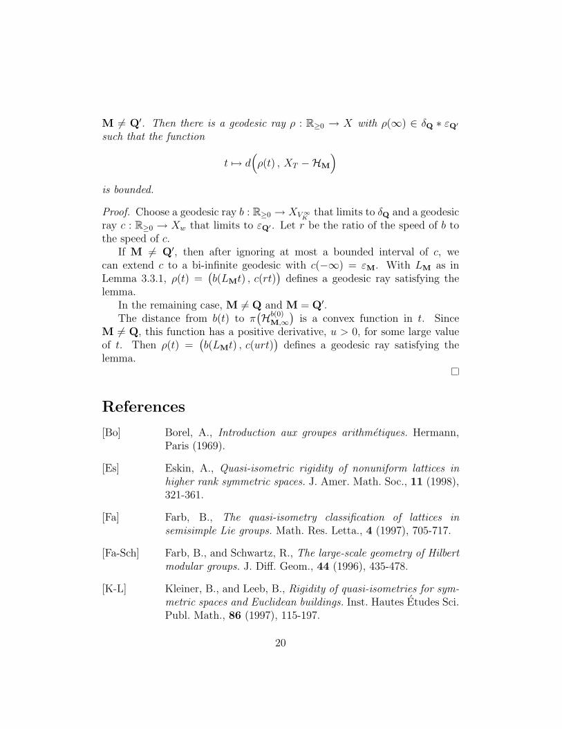
M 6= Q′. Then there is a geodesic ray ρ : R≥0 → X with ρ(∞) ∈ δQ ∗ εQ′such that the function

t 7→ d(ρ(t) , XT −HM

)is bounded.

Proof. Choose a geodesic ray b : R≥0 → XV∞Kthat limits to δQ and a geodesic

ray c : R≥0 → Xw that limits to εQ′ . Let r be the ratio of the speed of b tothe speed of c.

If M 6= Q′, then after ignoring at most a bounded interval of c, wecan extend c to a bi-infinite geodesic with c(−∞) = εM. With LM as inLemma 3.3.1, ρ(t) =

(b(LMt) , c(rt)

)defines a geodesic ray satisfying the

lemma.In the remaining case, M 6= Q and M = Q′.The distance from b(t) to π

(Hb(0)

M,∞)

is a convex function in t. SinceM 6= Q, this function has a positive derivative, u > 0, for some large valueof t. Then ρ(t) =

(b(LMt) , c(urt)

)defines a geodesic ray satisfying the

lemma.

References

[Bo] Borel, A., Introduction aux groupes arithmetiques. Hermann,Paris (1969).

[Es] Eskin, A., Quasi-isometric rigidity of nonuniform lattices inhigher rank symmetric spaces. J. Amer. Math. Soc., 11 (1998),321-361.

[Fa] Farb, B., The quasi-isometry classification of lattices insemisimple Lie groups. Math. Res. Letta., 4 (1997), 705-717.

[Fa-Sch] Farb, B., and Schwartz, R., The large-scale geometry of Hilbertmodular groups. J. Diff. Geom., 44 (1996), 435-478.

[K-L] Kleiner, B., and Leeb, B., Rigidity of quasi-isometries for sym-metric spaces and Euclidean buildings. Inst. Hautes Etudes Sci.Publ. Math., 86 (1997), 115-197.

20

[Sch 1] Schwartz, R., The quasi-isometry classification of rank one lat-tices. Inst. Hautes Etudes Sci. Publ. Math., 82 (1995), 133-168.

[Sch 2] Schwartz, R., Quasi-isometric rigidity and Diophantine approx-imation. Acta Math., 177 (1996), 75-112.

[Ta] Taback, J., Quasi-isometric rigidity for PSL2(Z[1/p]). DukeMath. J., 101 (2000), 335-357.

[Ta-Wh] Taback, J., and Whyte, K., The large-scale geometry of somemetabelian groups. Michigan Math. J. 52 (2004), 205-218.

[Ti] Tits, J., Classification of algebraic semisimple groups. 1966 Al-gebraic Groups and Discontinuous Subgroups (Proc. Sympos.Pure Math., Boulder, Colo., 1965) p. 33-62 Amer. Math. Soc.,Providence, R.I., 1966.

[Wo 1] Wortman, K., Quasi-isometric rigidity of higher rank S-arithmetic lattices. Geom. Topol. 11 (2007), 995-1048.

[Wo 2] Wortman, K., Quasi-isometric rigidity of higher rank arith-metic lattices over function fields. In appendix to: Einsiedler,M., and Mohammadi, A., A Joining classification and a spe-cial case of Raghunathan’s conjecture in positive charactersitic.Preprint.

Kevin WortmanDepartment of MathematicsUniversity of Utah155 South 1400 East, Room 233Salt Lake City, UT 84112-0090wortman@math.utah.edu

21