quasi newton methods for bound constrained...

MASTERARBEIT

Titel der Masterarbeit

“Quasi Newton Methods for BoundConstrained Problems”

Verfasser

Behzad Azmi

angestrebter akademischer Grad

Master of Science (MSc.)

Wien, im Juni 2012

Studienkennzahl lt. Studienblatt: A 066 821Studienrichtung lt. Studienblatt: Masterstudium MathematikBetreuer: o.Univ.-Prof. Dr. Arnold Neumaier

Acknowledgement

First and foremost, I would like to express my sincere gratitude to my advisor Prof.Arnold Neumaier for the continuous support of my Master’s study and research,for his patience, motivation, enthusiasm, and immense knowledge. His guidancehelped me in all the time of research and writing of this thesis. Special thanksgo to Prof. Hermann Schichl for his thoughtful guidance and for giving me theopportunity to work with them. I would also like to thank my beloved parents fortheir supporting and endless love, through the duration of my studies.

iii

Abstract

In this thesis, we are concerned with methods for solving large scale bound con-strained optimization problems. This kind of problems appears in a wide rangeof applications and plays a crucial role in some methods for solving generalconstrained optimization problems, variational inequalities and complementarityproblems. In the first part, we provide the general mathematical background of op-timization theory for bound constrained problems. Then the most useful methodsfor solving these problems based on the active set strategy are discussed. In sec-ond part of this thesis, we introduce a new limited memory quasi Newton methodfor bound constrained problems. The new algorithm uses a combination of thesteepest decent directions and quasi Newton directions to identify the optimal ac-tive bound constraints. The quasi Newton directions are computed using limitedmemory SR1 matrices and, if needed, by applying regularization. At the end, wepresent results of numerical experiments showing the relative performance of ouralgorithm in different parameter settings and in comparison with another algo-rithm.

iv

Zusammenfassung

Diese Arbeit befasst sich mit Methoden zur Losung von hochdimensionalen Opti-mierungsproblemen mit einfachen Schranken. Probleme dieser Art tauchen in ei-ner grossen Anzahl von unterschiedlichen Anwendungen auf und spielen eine ent-scheidende Rolle in einigen Methoden zur Losung von Optimierungsproblemenmit allgemeinen Nebenbedingungen, Variationsungleichungen und Komplemen-taritatsproblemen. Im ersten Teil dieser Arbeit beschreiben wir den allgemeinenmathematischen Hintergrund der Optimierungstheorie fur Optimierungsproblememit Schrankenbedingungen. Danach werden die nutzlichsten auf aktiven Mengenberuhenden Verfahren zur Losung dieser Probleme diskutiert. Im zweiten Teil die-ser Arbeit stellen wir ein neues Limited Memory Quasi Newton-Verfahren furhochdimensionale und einfach eingeschrankte Probleme vor. Der neue Algorith-mus verwendet eine Kombination aus den steilsten Abstiegsrichtungen und QuasiNewton Richtungen, um die Menge der optimalen aktiven Variablen zu identi-fizieren. Die Quasi Newton-Richtungen werden mit Hilfe der Limited MemorySR1 Matrizen und, falls erforderlich, durch die Anwendung einer Regularisie-rung berechnet. Zum Schluss prasentieren wir die Ergebnisse von numerischenExperimenten, die die relative Performance unseres Algorithmuses bezuglich un-terschiedlicher Parametereinstellungen und im Vergleich mit einem anderen Al-gorithmus darstellen.

v

Contents

1 Introduction 11.1 Formulation and Motivation . . . . . . . . . . . . . . . . . . . . 11.2 Preliminaries . . . . . . . . . . . . . . . . . . . . . . . . . . . . 2

2 Proposed Algorithms for Bound Constrained Problems 42.1 Introduction . . . . . . . . . . . . . . . . . . . . . . . . . . . . . 42.2 Standard Active-Set Method . . . . . . . . . . . . . . . . . . . . 42.3 The Gradient Projection Methods . . . . . . . . . . . . . . . . . . 7

2.3.1 Armijo Rule Along the Projection Arc . . . . . . . . . . . 82.3.2 Projected Search . . . . . . . . . . . . . . . . . . . . . . 9

2.4 Approaches for Quadratic Bound Constrained problems . . . . . . 112.4.1 BCQP . . . . . . . . . . . . . . . . . . . . . . . . . . . . 112.4.2 GPCG . . . . . . . . . . . . . . . . . . . . . . . . . . . . 14

2.5 A Trust Region Algorithm for Bound Constrained Problems . . . 172.5.1 Outline of the Algorithm . . . . . . . . . . . . . . . . . . 182.5.2 The Generalized Cauchy Point . . . . . . . . . . . . . . . 202.5.3 A Conjugate Gradient Type Method . . . . . . . . . . . . 242.5.4 The Algorithm . . . . . . . . . . . . . . . . . . . . . . . 27

2.6 L-BFGS-B . . . . . . . . . . . . . . . . . . . . . . . . . . . . . . 292.6.1 Outline of the Algorithm . . . . . . . . . . . . . . . . . . 302.6.2 Limited Memory BFGS Update . . . . . . . . . . . . . . 312.6.3 The Generalized Cauchy Point . . . . . . . . . . . . . . . 342.6.4 Subspace Minimization . . . . . . . . . . . . . . . . . . . 382.6.5 The Algorithm for L-BFGS-B . . . . . . . . . . . . . . . 45

3 A New Quasi Newton Method for Bound Constrained problems 473.1 Introduction . . . . . . . . . . . . . . . . . . . . . . . . . . . . . 473.2 Bent line Searches . . . . . . . . . . . . . . . . . . . . . . . . . . 473.3 Overview of the Algorithm . . . . . . . . . . . . . . . . . . . . . 513.4 Convergence Analysis . . . . . . . . . . . . . . . . . . . . . . . 533.5 Local Step . . . . . . . . . . . . . . . . . . . . . . . . . . . . . . 56

vi

CONTENTS

3.5.1 Limited Memory SR1 Update . . . . . . . . . . . . . . . 573.5.2 Computing the Search Direction . . . . . . . . . . . . . . 59

4 Numerical Experiments 644.1 Introduction . . . . . . . . . . . . . . . . . . . . . . . . . . . . . 644.2 Numerical Results . . . . . . . . . . . . . . . . . . . . . . . . . . 64

5 Conclusion and Future Work 71

Bibliography 72

vii

Chapter 1

Introduction

1.1 Formulation and MotivationIn this thesis we are concerned with method for solving the bound constrainedoptimization problem. Such a problem appears quite naturally in a wide rangeof applications including optimal design problem [5], contact and friction in rigidbody mechanics [19], the obstacle problem [22], journal bearing lubrication andflow through a porous medium [18]. Some approaches for solving variational in-equalities and complementarity problems have been proposed [1], in which theseproblems are reduced to bound constrained problems. Moreover, the bound con-strained optimization problem arises as a subproblem of the algorithms for solvinggeneral constrained optimization problems based on the augmented Lagrangianand penalty schemes [17, 16, 20]. In fact, some authors claim that each variablefor optimization problems can only be considered meaningful within a particu-lar interval [13]. These facts have motivated significant research dealing withdevelopment of efficient numerical algorithms for solving bound constrained op-timization problems, especially when the dimension of the problem is large.

The bound constrained optimization problems have the form

minimize f (x)subject to l ≤ x≤ u (1.1)

where the objective function f : Rn→ R is a sufficiently smooth function and thenumber of variables n is assumed to be large. Moreover, the fixed vectors l and uare lower and upper bounds on the variables respectively and the inequalities arecomponentwise.

The organization of this thesis goes as follows: In the rest of this chapter wereview some fundamental results of optimization theory in case of bound con-

1

Introduction

strained problems. Chapter 2 describes some effective methods used for solvinglarge scale bound constrained problems. In chapter 3 we introduce a new quasiNewton method for solving bound constrained problems. In chapter 4 we presentnumerical results demonstrating the relative performance of our algorithm in dif-ferent cases and in comparison to other algorithms. Finally, chapter 5 concludesthe thesis with directions for future work.

Throughout this thesis, we use the following notation. With the superscript Twe denote the transpose of a matrix(or vector), g and B represent the gradient andthe Hessian matrix of the objective function respectively.

1.2 PreliminariesFor solving problem (1.1), first, we need to characterize its solutions and theirproperties. In addition, once the solutions of the problem are mathematicallycharacterized, questions arise about the solution for example, whether it is uniqueor under which conditions it is the global minimizer of the problem. The followingtheorems and definitions answer these questions.

Theorem 1.2.1. Let F = {x ∈ Rn : l ≤ x ≤ u} be feasible region of (1.1) andsuppose that f is continuously differentiable on F with the gradient g.

1. If x∗ is the solution of (1.1) then

g(x∗)T (x− x∗)≥ 0, x ∈F . (1.2)

2. If f is convex on F then, conversely, every x∗ ∈F satisfying (1.2) is globalsolution of the (1.1).

3. The problem (1.1) has an unique solution x∗ whenever the objective functionf is strictly convex on feasible region F .

Proof. The proof of Abstract first order optimality conditions for general con-strained optimization problem [24, p, 97].

Theorem 1.2.2 (General first order optimality conditions for bound constrainedproblem). Let x∗ be the solution of (1.1), then there exist vectors λ ,µ ∈ Rn suchthat

g(x∗)−λ +µ = 0,

(x∗− l)Tλ = 0,

(u− x∗)Tµ = 0,

λ ,µ ≥ 0,

2

1.2 Preliminaries

where above conditions are called Karush-Kuhn-Tucker or KKT conditions andthey are equivalent to

gi(x∗)≥ 0, if x∗i = li,gi(x∗)≤ 0, if x∗i = ui,

gi(x∗) = 0, if li < x∗i < ui.

(1.3)

Proof. The proof of General first order optimality conditions [24, p, 105].

Note that the KKT conditions are necessary conditions for every solution of(1.1) but converse of above theorem does not hold unless, for example, the objec-tive function of (1.1) is convex in a neighbourhood of the feasible point satisfyingKKT conditions.

Definition 1.2.1. A point x∈F is said to be a stationary point for problem (1.1) ifit satisfies KKT conditions, or equivalently, the conditions (1.3) hold for x. More-over, strict complementarity is said to hold at x if the strict inequality hold in thefirst and second implications of (1.3).

In general, convergence to a stationary point is all that we can expect ofan algorithm for solving problem (1.1). In order to construct an algorithm forsolving (1.1) we need to characterize the stationary point in a more convenientway. Hence, if we define the reduced gradient of a feasible point x as a vectorgred = gred(x) with components

(gred)i : =

min(0,gi(x)) if xi = li,max(0,gi(x)) if xi = ui,

gi(x) if li < xi < ui,

(1.4)

a stationary point x can be characterized as

gred(x) = 0.

Definition 1.2.2. We call a stationary point x of (1.1) degenerate whenever thestrict complementarity fails to hold at x. In other words, there are some variablesxi ∈ {li,ui} with gi(x) = 0.

Degeneracy is a property of stationary points that causes difficulties for somealgorithms. When the strict complementarity does not hold at a solution of theproblem, there are some constraints of the problem that are weakly active at thesolution. In other words, all optimal Lagrange multipliers corresponding to theseconstraints are equal to zero. This fact makes it hard for an algorithm to find outwhether these constraints are active at the solution. Particularly, in the case ofactive-set methods and gradient projection methods this indecisiveness may causezigzagging, which means that the iterates of an algorithm move on and off theseweakly active constraints successively.

3

Chapter 2

Proposed Algorithms for BoundConstrained Problems

2.1 IntroductionIn this chapter we discuss several proposed algorithms for solving bound con-strained optimization problems. We begin this chapter by giving an overview ofthe standard active-set method. This method consists of two main steps. First,identifying the set of optimal active bound constraints or reaching the face con-taining a stationary point of the problem. Second, exploring the face of feasibleregion by solving an unconstrained subproblem. Then, we study the gradient pro-jection methods and their applications in the active-set methods. Indeed, all of thealgorithms described in this chapter deal with the bound constraints by explicitlydistinguishing between steps that search through the faces of the feasible regionand steps that explore the current face of the feasible region. The last two sectionsof this chapter are concerned with algorithms that, at each iteration, approximatethe objective function by a quadratic model whose Hessian matrix is computed bya limited memory method.

2.2 Standard Active-Set MethodIn this section we describe the standard active-set method for solving quadraticbound constrained optimization problems. A quadratic bound constrained prob-lem has the form

minimize f (x) = xT Bx+aT x,subject to l ≤ x≤ u, (2.1)

where B is symmetric and a belongs to Rn. Problem (2.1) is a special form ofthe (1.1), In addition, we will see later that some effective algorithms for solving

4

2.2 Standard Active-Set Method

(1.1) approximate the objective function of (1.1) with a quadratic model at eachiteration. Therefore, they rely on the solution of (2.1) at each iteration.

The standard active-set method for solving (2.1) finds step from one iterate tonext by solving an unconstrained quadratic subproblem in which some of variablesare fixed in one of their bounds. We call this subset of variables working set anddenote it at the kth iteration xk with Wk ⊂A (xk), where A (x) is the set of activevariables and defined by

A (x) = {i : xi = li∨ xi = ui}. (2.2)

We call variables with indices in Wk bound variables and other variables are re-ferred to as free variables. Now it is also helpful to define the binding set at x by

B(x) = {i : xi = li∧g(x)i ≥ 0, ∨ xi = ui∧g(x)i ≤ 0,}, (2.3)

where g(x) is the gradient of the objective function.

We assume that the initial point x0 is feasible and W0 ⊂A (x0). Now supposethat we are at the kth iteration with working set Wk, in order to compute xk+1 wesolve the following subproblem

minimize f (xk + p)subject to pi = 0, i ∈Wk.

(2.4)

The above problem is an unconstrained quadratic problem defined over the sub-space of free variables corresponding to Wk. Once the (2.4) is solved, we have twocases:

1. Problem (2.4) has a global solution pk. In this case if pk is zero, then xk isa global solution of the (2.1) over the working set Wk. Now assume that thevector pk is nonzero. For computing xk+1 we need to know how far we cango along pk while staying in the feasible region. If xk + pk is feasible withrespect to all bound constraints, we set xk+1 = xk + pk. Otherwise, we set

xk+1 = xk +αk pk,

where the step length αk is defined by

αk := min(

1, mini/∈wk∧pk

i >0

ui− (xk)i

pki

, mini/∈wk∧pk

i <0

li− (xk)i

pki

).

If αk < 1, that is, the step along direction pk is blocked by at least one ofthe bound constraints whose indices are not in Wk. Consequently, the newworking set Wk+1 is updated by adding atleast one of the constraints whichbecomes active at xk+1 to Wk.

5

Proposed Algorithms for Bound Constrained Problems

2. Problem (2.4) has no global solution. In this case it is possible to find thedirection pk such that the objective function of (2.4) is strictly decreasingand unbounded below along the ray xk +α pk for α > 0. In this case eitherf (x) is unbounded in the feasible region, or we set xk+1 = xk +αk pk, wherethe finite step length αk is defined by

αk := max{α ≥ 0 : l ≤ xk +α pk ≤ u}.

This means at least one bound constraints becomes active at xk+1.

In both of the cases once xk+1 is computed, Wk+1 is updated by adding at least oneof the blocking bound constraints to the Wk. Usually just one constraint is addedto the working set at each iteration.

We continue to iterate in the manner that outlined above, adding constraints tothe working set until we reach a point xt for t ≥ 1, which minimize the quadraticobjective function of (2.1) over the working set Wt . Equivalently, we keep iter-ating until pt = 0 is obtained as the global solution of the subproblem (2.4) withrespect to Wt .

After the global solution xt of subproblem (2.1) has been found we have twocases, either the working set Wt is a subset of B(xt), or there exist some indicesof Wt that do not belong to B(xt). If Wt is a subset of B(xt), then xt is a stationarypoint of (2.1) and algorithm terminates with xt . On the other hand, if there is aindex in Wt that does not belong to B(xt), the KKT conditions are not satisfied forxt , in particular, a Lagrange multiplier corresponding to an index in Wt is negative.Furthermore, by dropping this index from the working set the objective functionof (2.1) may be decreased. Therefore, we remove this index from the workingset and solve the subproblem (2.4) with a new working set. It can be shown by ashort computation that it is possible to find xt+1 with respect to the new workingset such that

f (xt+1)< f (xt).

If the quadratic function f (x) is bounded below on the feasible region, it isnot difficult to show that the active-set method converges to a stationary pointin a finite number of iterations. Our argument for verifying this result is quiteinstructive. At each iteration either we reach a global minimizer of the subproblemor we increase the size of the working set. Because the cardinality of working setis always bounded by n, the global solution of (2.4) will be obtained after at mostn iterations. On the other hand, if the global solution xt of the subproblem isdetermined with respect to some working set Wk, then xt is a global solution of thef (x) subject to the face of the feasible region which is defined by

{x ∈ Rn : l ≤ x≤ u,xi ∈ {li,ui}, i ∈Wt}. (2.5)

6

2.3 The Gradient Projection Methods

Since f (xt+1)< f (xt), it is impossible for the algorithm to arrive in this face againin an iteration xr with r > t. Moreover, the number of possible faces is finite, thusthe active set method terminates in a finite number of iterations.

Finally, we summarize the active-set method in two main steps:

Global Step: If xt is a global solution of the f (x) subject to the face (2.5), thenfind a feasible point xt+1 such that f (xt+1)< f (xt) . Indeed, in this step wemove from a face to another until we land on the face that contains a globalsolution of (2.1).

Local Step: Otherwise find a feasible point xt+1 such that f (xt+1) ≤ f (xt) andWt ⊂Wt+1. If Wt =Wt+1 then xt+1 must be a global solution of f (x) subjectto the face (2.5). In this step we explore the face of the feasible region whichis defined by the current working set.

As it has been mentioned, the standard active-set method drops only one con-straint from the current working set in the global step and adds only one constraintto the current working set in the local step. That is, at each step of the standardactive-set method, the dimension of the subspace of bound variables is changedonly by one. This fact implies that if there are n1 active constraints on x0 and n2active constraints on the solution of (2.1), we need at least |n2− n1| iterations toreach the solution of (2.1). This may be serious drawback in the case of large scaleproblems. This observation motivated many authors, specially BERTSEKAS [2],to use gradient projection method for solving bound constrained problems. He hasestablished that the set of active constraints at the nondegenerate stationary pointof bound constrained problem (1.1) is identified in a finite number of iterations byusing gradient projection method. We will see later how the gradient projectionmethod and active-set method are combined with each others in order to constructan efficient algorithm for solving bound constrained problems.

2.3 The Gradient Projection MethodsIn this section we begin with an overview of the gradient projection methods forsolving general optimization problems with the form

minimize f (x)subject to x ∈F

(2.6)

where f :Rn→R is continuously differentiable and F is a convex feasible region.

7


Given an iterate xk, the next iterate xk+1 is computed by the gradient projectionmethod as follows

xk+1 = PF [xk−αkg(xk)].

Where PF [x] is the orthogonal projection on the feasible region F , g(x) is the gra-dient of objective function, and the step length αk > 0 is chosen so that f (xk+1)<f (x). The projection part plays important rule in the gradient projection methodand it must be computed in a fairly simple way. Otherwise, it does not makepractical sense to use the gradient projection method. In general the orthogonalprojection on the feasible region has the form

PF [x] = arg miny∈F‖x− y‖. (2.7)

The computation of (2.7) for general constrained optimization problems can beexpensive but in the case of bound constrained problems with F = {x ∈ Rn : l ≤x≤ u}, it requires only order of n operations and it is defined by

(PF [x])i = (P[x, l,u])i =

li if xi ≤ li,ui if xi ≥ ui,

xi if li < xi < ui.

(2.8)

It can be shown that by choosing an appropriate step length αk, the gradientprojection method is able to identify the set of active constraints at the nondegen-erate stationary point in finite number of iterations. This is a consequence of thefact that if x is a nondegenerate stationary point of the problem, then there existsa neighbourhood N (x) of x such that A (xk+1) = A (PF [xk−αkg(xk)]) providedxk ∈N (x). This identification ability of the gradient projection method is validaccording to [12, 2, 8]. Now we describe some methods for computing the steplength αk, in which the gradient projection method has this identification ability.

2.3.1 Armijo Rule Along the Projection ArcThis procedure was proposed by BERTSEKAS [3, 4] and its concept is really sim-ple. First we chose the fixed scalers α , β , and σ > 0, with α > 0, β ∈ (0,1), andσ ∈ (0,1). Then we define the following piecewise linear path

xk(α) := PF [xk−αg(xk)], α > 0, (2.9)

where P is the projection into the feasible region F and g represents the gradientof the objective function. Finally the step length αk is determined by propor-tionally reduction of the α with a factor β ∈ (0,1) until the Armijo condition

8

2.3 The Gradient Projection Methods

is satisfied. In other words, we set αk = β rkα , where rk is the first nonnegativeinteger r for which the following conditions holds.

f (xk)− f (xk(βrα))≥ σg(xk)

T (xk− xk(βrα)). (2.10)

It can be shown that the above step-size rules is well defined, That is, after a finitenumber of trials based on the (2.10) the steplength αk will be found. Further-more, the gradient projection method with the above linesearch procedure is ableto identify the set of active constraints at the nondegenerate solution of the (2.6)in finite iterations.

2.3.2 Projected SearchThe projected search is a procedure for finding αk for the case in which f (x) =xT Bx+aT x and the feasible region F consisting of bound constraints. This pro-cedure was proposed by MORE and TORALDO [21, 22]. In this procedure thecomputation of αk relies on the function defined by

φk(α) := f (PF [xk +α pk]), (2.11)

where P is the projection (2.8) into the bound constraints and pk is a search di-rection with φ ′k(0) < 0. We determine a step-length αk > 0 so that the sufficientdecrease condition holds for φk(α). The sufficient decrease condition is definedby

φk(αk)≤ φk(0)+σg(xk)T (PF [xk +α pk]− xk), (2.12)

where σ ∈ (0, 12) is fixed. Since the path PF [xk +α pk] is a linear function on

any interval on which the set of active constraints at PF [xk +α pk] is unchanged,φk(α) is a continuous piecewise quadratic function. For defining Breakpoints forφk(α) we compute

0 = t1 < t2 < ... < tm < tm+1 =+∞

so that A (PF [xk +α pk]) is unchanged on the intervals (ti, ti+1) for i = 0, ...,m. Ifwe allow infinite value for li or ui, it is possible to have m = 0 in the computationsof breakpoints. Moreover, the first breakpoint has a interesting feature, namely itcan be shown that there is α ∈ [0, t1] that satisfies the sufficient decrease condition(2.12) and for all α ∈ [0, t1] we have also

φk(α) = f (PF [xk +α pk]) = f (xk +α pk), (2.13)

where pk is given from pk by taking the components whose indices correspondto the free variables at xk. Similarly, we define matrix Bk which is obtained from

9


B by choosing the rows and columns whose indices are corresponding to the freevariables. To put it another way, if Zk denotes the matrix whose columns span thesubspace of free variables at xk, we have

pk = ZTk pk, Bk = ZT

k BZk.

The projected search method generate a positive decreasing sequence {αrk}r of

trial values until a trial value is found which satisfies (2.12). Note that this processwill terminate after a finite number of steps, since there exists a trial value in theinterval [0, t1] which fulfils (2.12).

Now for choosing the initial trial value α0k we have two cases depending on

the behaviour of φk on the interval [0, t1]:

1. φk is strictly convex on the [0, t1]. In this case the initial trial value is givenby the first minimizer of the quadratic function φk(α) in [0, t1] and computedby

α0k =−φ ′k(0)φ ′′k (0)

=‖pk‖2

pTk Bk pk

,

where pTk Bk pk > 0. Note that if α0

k < t1, the procedure terminates with theacceptable step length αk = α0

k .

2. φk is not strictly convex on [0, t1] and also pTk Bk pk ≤ 0. In this case the

quadratic function φk(α) is on [0, t1] strictly decreasing and unbounded be-low. Consequently, it is better to choose α0

k desirable large. Hence, weset

α0k = tm.

Now suppose that the initial trial value α0k is given. If it satisfies (2.12), we ter-

minate with αk = α0k . Otherwise, given the current trial value αr

k with r > 1, forwhich the (2.12) is not satisfied. For computing the new trial value, we determinethe minimizer of the quadratic approximation that interpolates the pieces of in-formation φk(0), φ ′k(0), and φk(α

rk). Then the new trial value α

r+1k is given by

max(t1,mid(0.01αrk , α,0.5α

rk)), (2.14)

where mid(0.01αrk , α,0.5αr

k) is the middle element of the set {0.01αrk , α,0.5αr

k}.The above process is continued until a trial value satisfying (2.12) is found. Thefinite termination is also guaranteed. Since, if either pT

k Bk pk ≤ 0 or α0k > t1, t1

satisfies the sufficient condition with σ ≤ 0.5.

Note that for the projection gradient method, we use −g(xk) as the searchdirection pk at each iteration.

10

2.4 Approaches for Quadratic Bound Constrained problems

2.4 Approaches for Quadratic Bound Constrainedproblems

In this section we will deal with the algorithms for solving bound constrainedquadratic problems (2.1). As we have mentioned, the standard active-set methodhas the major disadvantage that at each iteration the cardinality of the workingset is changed by dropping or adding only one constraint. On the other hand, aswe have discussed in the previous section, the gradient projection method is ableto identify the set of optimal active set in finite number of iterations. This factsmotivated many authors, for example, MORE and TORALDO [21, 22] to proposealgorithms that use the gradient projection method in an efficiently manner inthe active-set method schema. Particularly, these algorithms take advantage ofthe identification property of the gradient projection method to reach the facecontaining the solution quickly, and to explore each face of the feasible region,they solve an unconstrained optimization subproblem (2.4).

2.4.1 BCQP

This algorithm is proposed by MORE and TORALDO [21] to solve the quadraticbound constrained problem (2.1) and it consists of two main steps:

Global Step: Set xk = u0 and generate the iterations u0,u1, ...,us by the gradi-ent projection method. If for some j ∈ {1, ...,s} the condition A (u j) =A (u j−1) is satisfied then we set xk+1 = u j. Otherwise, we set xk+1 = us.

Local Step: Otherwise find a feasible xk+1 such that f (xk+1) ≤ f (xk) and Wk ⊂Wk+1. If Wk = Wk+1 then xk+1 must be a global solution of f (x) subject tothe face {x ∈ Rn : l ≤ x≤ u,xi ∈ {li,ui}, i ∈Wk}.

As we can see, the only deference of the above algorithm and the standard active-method is in the global step. Indeed, the gradient projection method is used inthe global step to modify the standard active-set method in two aspects. Firstly,the cardinality of the working set is changed by dropping and adding many con-straints. Secondly, the algorithm tends to find the optimal active constraints morequickly.

It should be noted that, in the global step the gradient projection method isperformed with the help of projected search method 2.3.2. That is, a sequence{u j} is computed by

u j+1 = PF [u j−α jg(u j)],

11


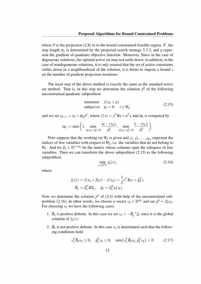
where P is the projection (2.8) in to the bound constrained feasible region F , thestep length α j is determined by the projected search strategy 2.3.2, and g repre-sent the gradient of quadratic objective function. Moreover, Since in the case ofdegenerate solutions, the optimal active set may not settle down, in addition, in thecase of nondegenerate solutions, it is only assured that the set of active constraintssettles down in a neighbourhood of the solution, it is better to impose a bound son the number of gradient projection iterations.

The local step of the above method is exactly the same as the standard activeset method. That is, in this step we determine the solution pk of the followingunconstrained quadratic subproblem

minimize f (xk + p)subject to pi = 0, i ∈Wk.

(2.15)

and we set xk+1 = xk +αk pk, where f (x) = xT Bx+aT x and αk is computed by

αk := min(

1, mini/∈wk∧pk

i >0

ui− (xk)i

pki

, mini/∈wk∧pk

i <0

li− (xk)i

pki

).

Now suppose that the working set Wk is given and j1, j2, . . . , jmk represent theindices of free variables with respect to Wk, i.e. the variables that do not belong toWk. And let Zk ∈ Rn×mk be the matrix whose columns span the subspace of freevariables. Then we can transform the above subproblem (2.15) to the followingsubproblem.

minv∈Rmk

fk(v), (2.16)

where

fk(v) = f (xk +Zkv)− f (xk) =12

vT Bkv+ gTk v,

Bk = ZTk BZk, gk = ZT

k g(xk).

Now we determine the solution pk of (2.4) with help of the unconstrained sub-problem (2.16), In other words, we choose a vector vk ∈ Rmk and set pk = Zkvk.For choosing vk we have the following cases:

1. Bk is positive definite. In this case we set vk =−B−1k g, since it is the global

solution of fk(v).

2. Bk is not positive definite. In this case vk is determined such that the follow-ing conditions hold

vTk Bkvk ≤ 0, gT

k vk ≤ 0, min{vTk Bkvk, gT

k vk}< 0 (2.17)

12


This is possible whenever Bk is either not positive semidefinite or regular,or gk /∈ Im(Bk)

The computation of vk is based on the Cholesky factorization of Bk and weneed almost one factorization for all matrices. If Bk is positive definite then theCholesky factorization of the matrix exists and is used for computing vk. Other-wise, while computing of Cholesky factorization we try to find the largest positivedefinite principal minor of the matrix. Let this principal minor has the order land be represented by Ck, then the principal minor of order l + 1 of Bk has thefollowing form (

Ck wkwT

k θk

)(2.18)

Due to positive definiteness, Ck has a Cholesky factorization RTk Rk. Now we claim

thatθk ≤ wT

k C−1k wk. (2.19)

Suppose on contrary that (2.19) does not hold, then it is easy to verify that theCholesky factorization of (2.18) is(

RTk 0

qTk ηk

)(Rk qk0 ηk

),

whereRT

k wk = qk, ηk = (θk−‖qk‖2)12 = (θk−wT

k C−1k wk)

12 .

But this is contradiction with the fact that (2.18) is not positive definite. Therefore(2.19) holds. Consequently, if we define the vector vk ∈ Rmk by

vk =±(C−1k wk,−1,0, . . . ,0),T

where the sign of vk is chosen such that vT gk ≤ 0, we have

vTk Bkvk = θk−wT

k C−1k wk ≤ 0.

This shows that (2.17) is satisfied, provided either vTk gk 6= 0 or vT

k Bkvk 6= 0.

It should be noted that if for vk the condition (2.17) is satisfied, then thepk = Zkvk defines a direction such that f (xk + α pk) is strictly decreasing andunbounded below for α > 0. Hence, similar to the standard active-set method,either f is unbounded below on the feasible region or a finite αk corresponding toa blocking constraint is computed.

The BCQP algorithm terminates at the iterate xk if one of the following casesoccurs:

13


1. The matrix Bk is positive semidefinite, gk = 0, and Wk ⊂ B(xk). In thiscase the vector pk = 0 is the global solution of the unconstrained quadraticsubproblem (2.15) with respect to the working set Wk. In addition, becauseWk is a subset of B(xk), iterate xk is a stationary point of the problem.

2. For all α > 0, the ray xk +α pk is feasible and the function f (xk +α pk) isdecreasing and unbounded below.

3. For all α > 0, the ray xk +α pk is feasible and the function f (xk +α pk) isconstant and pk = 0. In this case we have two possible situations, either f (x)is unbounded below on the feasible region, or there exists a arbitrary smallperturbation on the gk or Bk which leads to the fact that f is unbounded onthe feasible region.

Moreover, in [21, p. 388] it has been shown that if the quadratic objective func-tion f : Rn→R is bounded from the below on the feasible region, then the BCQPalgorithm terminate at a stationary point in finite iteration steps.

It should be mentioned that in the global step of the BCQP, only one constraintis added to the working set. This can be serious disadvantage for large scaleproblems, hence we aim to construct an algorithm that is able to add many variableto the working set in the global step.

2.4.2 GPCGIn this section we present an algorithm to find the solution of (2.1), where thequadratic function f is strictly convex, i.e. the matrix B in (2.1) is positive definite,and the number of variable is assumed to be large. This algorithm was developedby MORE and TORALDO [22]. Similar to the standard active-method and BCQP,this method generates a sequence of iterations xk that terminates at a solution of(2.1) in finite number of iterations. Moreover, the termination typically is obtainby solving a sequence of unconstrained quadratic subproblems of the form

minimize f (xk + p)subject to pi = 0, i ∈Wk

(2.20)

with a working set Wk, and changing the size of working set by dropping andadding constraints at each iteration. In particular, this algorithm performs the gra-dient projection method until either an adequate working set Wk is identified orthe gradient projection method is no longer able to deliver an acceptable improve-ment. Furthermore, the conjugate gradient method is applied to find approximatesolution of the above unconstrained subproblem with respect to the current Wk.

14


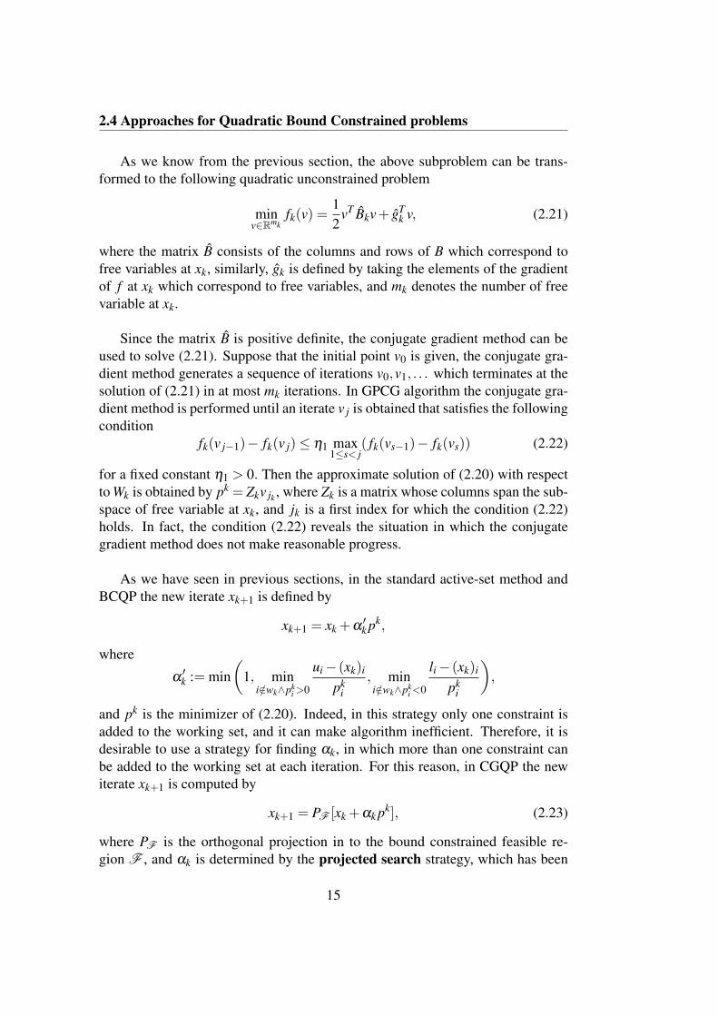
As we know from the previous section, the above subproblem can be trans-formed to the following quadratic unconstrained problem

minv∈Rmk

fk(v) =12

vT Bkv+ gTk v, (2.21)

where the matrix B consists of the columns and rows of B which correspond tofree variables at xk, similarly, gk is defined by taking the elements of the gradientof f at xk which correspond to free variables, and mk denotes the number of freevariable at xk.

Since the matrix B is positive definite, the conjugate gradient method can beused to solve (2.21). Suppose that the initial point v0 is given, the conjugate gra-dient method generates a sequence of iterations v0,v1, . . . which terminates at thesolution of (2.21) in at most mk iterations. In GPCG algorithm the conjugate gra-dient method is performed until an iterate v j is obtained that satisfies the followingcondition

fk(v j−1)− fk(v j)≤ η1 max1≤s< j

( fk(vs−1)− fk(vs)) (2.22)

for a fixed constant η1 > 0. Then the approximate solution of (2.20) with respectto Wk is obtained by pk = Zkv jk , where Zk is a matrix whose columns span the sub-space of free variable at xk, and jk is a first index for which the condition (2.22)holds. In fact, the condition (2.22) reveals the situation in which the conjugategradient method does not make reasonable progress.

As we have seen in previous sections, in the standard active-set method andBCQP the new iterate xk+1 is defined by

xk+1 = xk +α′k pk,

where

α′k := min

(1, min

i/∈wk∧pki >0

ui− (xk)i

pki

, mini/∈wk∧pk

i <0

li− (xk)i

pki

),

and pk is the minimizer of (2.20). Indeed, in this strategy only one constraint isadded to the working set, and it can make algorithm inefficient. Therefore, it isdesirable to use a strategy for finding αk, in which more than one constraint canbe added to the working set at each iteration. For this reason, in CGQP the newiterate xk+1 is computed by

xk+1 = PF [xk +αk pk], (2.23)

where PF is the orthogonal projection in to the bound constrained feasible re-gion F , and αk is determined by the projected search strategy, which has been

15


described in the subsection 2.3.2. Note that if αk > α ′k, then more than one con-straint might be added to the working set.

Now assume that a new iteration xk+1 has been computed by the conjugategradient method. If xk+1 is in the face containing the solution of problem, thisface will be explored further by the conjugate gradient method. This decision ismade in terms of verifying the following condition

A (xk+1) = B(xk+1), (2.24)

where A (x), B(x) denote, respectively, the set of active and binding variables atx. Note that, if xk+1 is in the face containing the solution, the condition (2.24)holds.

Remark 2.4.1. Note that if (2.24) holds, it does not necessarily mean that xk+1 isin the face that contains the solution of the problem. Nevertheless, if xk+1 is notin this face, because of the finite termination property of the conjugate gradientmethod, an iterate xr with r > k + 1 is eventually generated which violates thecondition A (xr) = B(xr).

Once a face has been explored by conjugate gradient method, the gradientprojection method is used to search through the different faces by generating asequence {u j} which is defined by

u j+1 = PF [u j−α jg(u j)],

where P is the projection (2.8) in to the bound constrained feasible region F , thestep length α j is determined by the projected search strategy 2.3.2, and g denotesthe gradient of the quadratic objective function. The gradient projection methodis used to choose a new face as follows: assume that we are at the kth iterationwith xk, we set u0 = xk and generate iterations u0,u1,u3, . . . until for some fixedη2 one of the following conditions

A (u j) = A (u j−1), (2.25)f (u j−1)− f (u j)≤ η2 max

1≤s< j( fk(us−1)− fk(us)) (2.26)

is satisfied. The justification of the condition (2.25) is based on the result whichsays, in the case of nondegenerate problems there exists a neighbourhood of thesolution such that the condition (2.25) is satisfied provided that xk belongs to thisneighbourhood. Furthermore, the condition (2.26) prevents the gradient projec-tion method from making deficient progress.

The above description can be summarized in to the following steps:

16

2.5 A Trust Region Algorithm for Bound Constrained Problems

Global step: Generate a sequence u0,u1,u2, . . . with u0 = xk by the gradient pro-jection method. Set xk+1 = u jk , where jk is the first index j which fulfilseither (2.25) or (2.26).

Local step: Generate a sequence v0,v1,v2, . . . by the conjugate gradient methodwith v0 = 0 in order to solve (2.21) approximately. Then set pk = Zkv jk ,where jk is the first index that fulfils (2.22). Use the projected search strat-egy to determine the step length αk and define xk+1 by (2.23). If (2.24) issatisfied, continue the conjugate gradient method.

It is claimed in [22] that if the termination of GPCG is occurred in a finite numberof iterations, then it terminates at the solution of the problem. If the terminationoccurs in the global step, duo to standard result of the gradient projection methodit terminates at the solution of the problem. Moreover, In local step the termina-tion can only occur if the conjugate gradient method generates an iterate xs withgs = 0 and A (xs) = B(xs). Which implies that gred(xs) = gs = 0, so xs is thesolution.

The main theoretical result for convergence of GPCG is based on the followingtheorem which is represented in [22, p, 101]:

Theorem 2.4.1. Suppose that f : Rn→ R is a strictly convex quadratic function.If xk is the sequence generated by GPCG for solving the problem (2.1), then eitherxk terminates at the solution x∗ of the problem (2.1) in a finite number of iterations,or xk converges to the solution x∗.

2.5 A Trust Region Algorithm for Bound ConstrainedProblems

In this section we describe a method of trust region type for solving problem(1.1), where the objective function f : Rn→R is a arbitrary function which is suf-ficiently smooth. We have no convexity assumption on f . Recall that the feasibleregion is the set of all x ∈ Rn for which l ≤ x≤ u.

This method proposed by CONN, GOULD and TOINT [10, 9] is a combinationof the active set method strategy and trust region method. That is, at each iterationof this algorithm, the objective function is approximated by a quadratic modelwithin a region surrounding the current iteration. Then the algorithm chooses anew feasible point in that region for the next iterate such that it gives a sufficientdecrease in the value of the quadratic model. If the value of objective functionat this point decreases sufficiently as it is predicted by the quadratic model, then

17


the computed feasible point within the region is accepted as the next iterate andthe algorithm expands the region. Otherwise, the algorithm rejects this point andshrinks the region. Moreover, the set of active constraints changes in this methodrapidly. The general convergence theory of this method is presented in [9].

2.5.1 Outline of the AlgorithmBefore describing the method, we define the active set at point x with respectto vectors l and u as the set of all indices i ∈ {1, . . . ,n} for which either xi ≤ lior xi ≥ ui,. We denote this set with A (x) = A (x, l,u). Furthermore, P[x, l,u]represents the projection on to the set {x ∈ Rn : l ≤ x≤ u} computed by

(P[x, l,u])i =


xi if li < xi < ui.

Now suppose that we are at the kth iteration with xk, the gradient gk of theobjective function f at xk. The objective function f is approximated at xk bya quadratic model mk whose gradient coincides with gk, and whose symmetricHessian matrix Bk is computed by a limited memory quasi Newton method. Inaddition, we need a scaler ∆k as the radius of the trust region at the kth iteration,i.e. a bound on the displacement around xk. we believe that in this region thebehaviour of the quadratic model

mk(x+ p) = f (xk)+gTk p+

12

pT Bk p, s.t. ‖p‖ ≤ ∆k (2.27)

is similar to the objective function. Then a trial point xk+1 = xk + pk for next iter-ation is determined by finding an approximation to the solution of the followingtrust region problem

minimize mk(x)subject to l ≤ x≤ u,

‖x− xk‖ ≤ ∆k,

(2.28)

where ‖.‖ is the infinity norm. The acceptance of the trial point xk+1 as the newiterate and the modification of the trust region radius ∆k are based on the agree-ment of the quadratic model mk with the objective function f at the iteration xk.That is, we compute the following ratio

ρk :=f (xk)− f (xk + pk)

mk(xk)−mk(xk + pk), (2.29)

18


where the numerator and dominator of (2.29) are called actual and predicted re-duction, respectively. Then we set

xk+1 =

{xk + pk if ρk > µ,

xk if ρk ≤ µ,

and modify the radius ∆k as follows

∆k+1 =

γ1∆k if ρk ≤ µ,

∆k if µ < ρk < η ,

γ2∆k if ρk ≥ η ,

(2.30)

where 0 < γ1 < 1 < γ2, µ and η are fixed numbers. Now we describe how thesolution of (2.28) is approximated at each iteration. Since ‖.‖ in (2.28) is theinfinity norm, the shape of the trust region is like a box. Hence, we can transform(2.28) to the following bound constrained problem

minimize mk(x)subject to lk ≤ x≤ uk,

(2.31)

where

(lk)i :=max(li,(xk)i−∆k),

(uk)i :=min(ui,(xk)i +∆k),(2.32)

for all i ∈ {1, . . . ,n}.

According to [9], in order to fulfil the global convergence theory, it is requiredto find a feasible point of (2.31) at which the value of the quadratic model mk is notgreater than its value at the generalized Cauchy point (CP). Where the generalizedCauchy point is defined as the first local minimizer of the following univariate,piecewise quadratic function

qk(t) := mk(P[xk− tgk, lk,uk]). (2.33)

In other words, the CP is the first minimizer of the quadratic model mk along thepiecewise linear path P[xk− tgk, lk,uk] which is defined by projecting the steepestdescent direction into the region

{x ∈ Rn : lk ≤ x≤ uk}.

Note that the generalized Cauchy point is a kind of the gradient projection meth-ods that we have described in section (2.3). Therefore, it allows the algorithm to

19


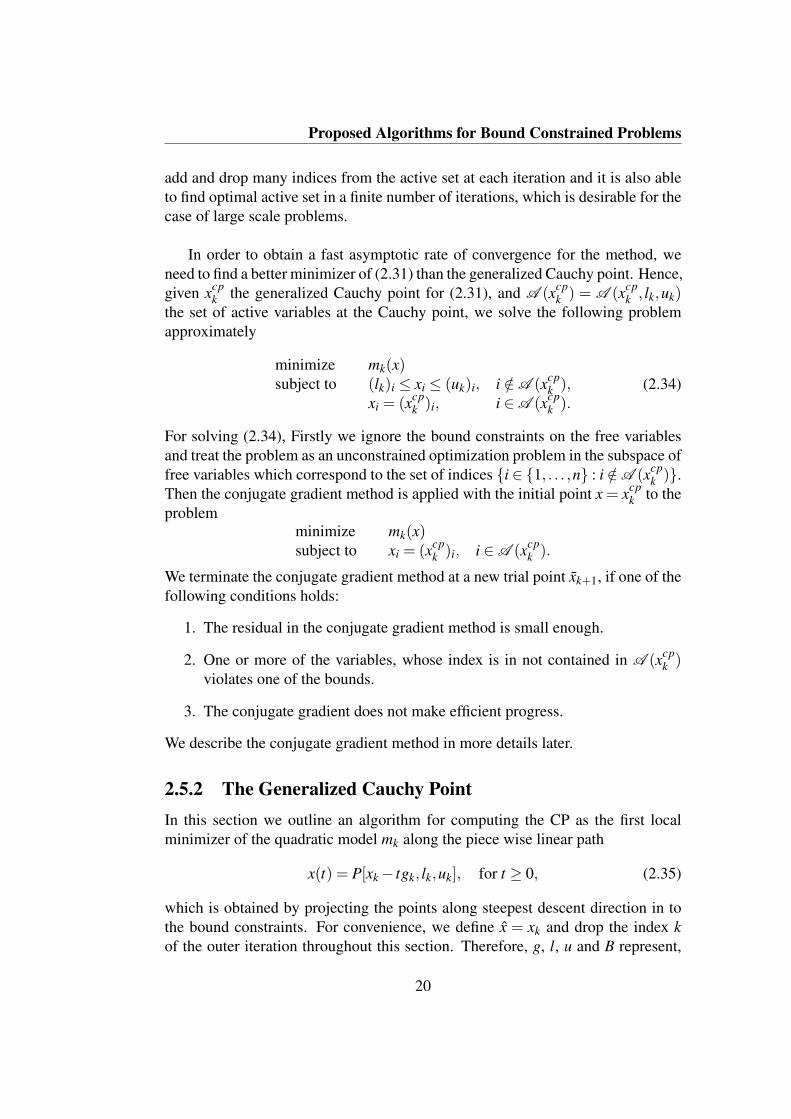
add and drop many indices from the active set at each iteration and it is also ableto find optimal active set in a finite number of iterations, which is desirable for thecase of large scale problems.

In order to obtain a fast asymptotic rate of convergence for the method, weneed to find a better minimizer of (2.31) than the generalized Cauchy point. Hence,given xcp

k the generalized Cauchy point for (2.31), and A (xcpk ) = A (xcp

k , lk,uk)the set of active variables at the Cauchy point, we solve the following problemapproximately

minimize mk(x)subject to (lk)i ≤ xi ≤ (uk)i, i /∈A (xcp

k ),xi = (xcp

k )i, i ∈A (xcpk ).

(2.34)

For solving (2.34), Firstly we ignore the bound constraints on the free variablesand treat the problem as an unconstrained optimization problem in the subspace offree variables which correspond to the set of indices {i ∈ {1, . . . ,n} : i /∈A (xcp

k )}.Then the conjugate gradient method is applied with the initial point x = xcp

k to theproblem

minimize mk(x)subject to xi = (xcp


We terminate the conjugate gradient method at a new trial point xk+1, if one of thefollowing conditions holds:

1. The residual in the conjugate gradient method is small enough.

2. One or more of the variables, whose index is in not contained in A (xcpk )

violates one of the bounds.

3. The conjugate gradient does not make efficient progress.

We describe the conjugate gradient method in more details later.

2.5.2 The Generalized Cauchy PointIn this section we outline an algorithm for computing the CP as the first localminimizer of the quadratic model mk along the piece wise linear path

x(t) = P[xk− tgk, lk,uk], for t ≥ 0, (2.35)

which is obtained by projecting the points along steepest descent direction in tothe bound constraints. For convenience, we define x = xk and drop the index kof the outer iteration throughout this section. Therefore, g, l, u and B represent,

20


respectively, gk, lk, uk and Bk. Subscripts are used to denote the components of avector.

For deriving an explicit expression for piece wise linear path (2.35), we definethe breakpoints in each coordinate by

ti :=

xi−ui

giif gi < 0

xi−ligi

if gi > 0

∞ otherwise,

(2.36)

and we sort breakpoints ti for i = 1, . . . ,n in an ascending order to obtain theordered set {t j : t j ≤ t j+1, j = 1, . . . ,n}. Then the piecewise linear search path x(t)can be expressed by

xi(t) =

{xi− tgi if t ≤ tixi− tigi if t > ti,

(2.37)

which is linear on each interval [t j, t j+1] with j = 1, . . . ,n−1. For finding the CPwe examine the intervals [0, t1], [t1, t2], [t2, t3], . . . in turn until the one that containsthe CP is located.

Assume that we have examined the intervals [tk−1, tk] for k = 1, . . . , j and de-termined that the local minimizer lies at some value t ≥ t j. Now we are examiningthe interval [t j, t j+1]. We define the jth breakpoint by

x j = x(t j).

Hence, on the interval [t j, t j+1] we have

x(t) = x j +∆td j, (2.38)

where∆t = t− t j, ∆t ∈ [0, t j+1− t j], (2.39)

and

d ji =

{−gi if t j < ti0 otherwise.

(2.40)

In order to compute the generalized Cauchy point, we need to investigate thebehaviour of the quadratic model

m(x) = f (x)+gT (x− x)+12(x− x)T B(x− x) (2.41)

21


for points lying on the interval [t j, t j+1]. By substituting (2.38) in (2.41), we canexpress the quadratic model m on the line segment [x(t j),x(t j+1)] as

m(x) = f (x)+gT (v j +∆td j)+12(v j +∆td j)T B(v j +∆td j),

wherev j = x j− x. (2.42)

Consequently, m can be written as a quadratic function in ∆t,

m(∆t) =( f (x)+gT v j +12(v j)T Bv j)+(gT d j +(d j)T Bv j)∆t

+((d j)T Bd j)∆t2.

By expanding and grouping the coefficients 1, ∆t, and ∆t2 we can write the aboveone dimensional quadratic function m as

m(∆t) = f j + f ′j∆t +12

f ′′j ∆t2, (2.43)

where the coefficients f j, f ′j, and f ′′j are determined by

f j := f (x)+gT v j +12(v j)T Bv j,

f ′j :=gT d j +(d j)T Bv j, (2.44)

f ′′j :=(d j)T Bd j. (2.45)

By differentiating m with respect to ∆t and setting it to zero, we obtain ∆t∗ =− f ′j/ f ′′j . Now we have these cases:

• If f ′′j > 0 and ∆t∗ ∈ [0, t j+1− t j], we deduce that there exists a local mini-mizer of m(x(t)) at t = t j +∆t∗. Hence, the CP lies at x(t j +∆t∗).

• Otherwise, the CP lies at x(t j), provided that we have f ′j > 0.

• In all other cases the CP lies at x(t j+1) or outside of interval [t j, t j+1]. There-fore, we continue to search through the next interval. In these cases we needto calculate the new direction d j+1 from (2.40), and use this vector for cal-culating f j+1, f ′j+1 and f ′′j+1. Since the difference between d j and d j+1 istypically in just one component, we can made computational save by updat-ing the coefficients f j+1, f ′j+1 and f ′′j+1 rather than calculating them fromthe scratch.

22


Now we need to be concerned with computing f ′j+1 and f ′′j+1. Assume thatI is the set of indices corresponding to the variables that become active att j+1. That is,

I j+1 := {i ∈ {1, . . . ,n} : ti = t j+1}. (2.46)

Then we haved j+1 = d j− ∑

k∈I j+1

dkek,

where ek is the kth column of the identity matrix. Now we can compute

f ′j+1 = f ′j +∆ j f ′′j − (b j+1)T x j+1− ∑k∈I j+1

dkg′k,

f ′′j+1 = f ′′j +(b j+1)T(

∑k∈I j+1

dkek−2d j),

(2.47)

where g′ := g−Bx, ∆t j := t j+1− t j and

b j+1 := B( ∑k∈I j+1

dkek) = ∑k∈I j+1

dk(Bek). (2.48)

Note that the computations (2.47) need only a matrix-vector multiplication(2.48) and two inner products of vectors. Furthermore, the matrix-vectormultiplication includes columns of B which are indexed by I j+1. Since|I j+1| is usually small, the product can be done very efficiently.

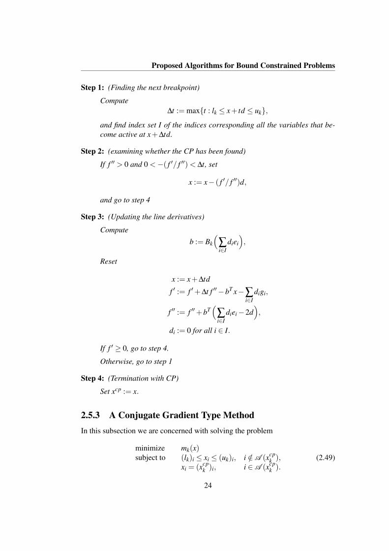
Now we give an algorithm for computing the generalized Cauchy point.

Algorithm 2.5.1. Generalized Cauchy Point

Step 0: (Initialization)

Given xk, lk, l,uk,u,gk, and Bk, Initialize

x := xk,

g := gk−Bkxk

d := limt→0+

P[xk− tgk, l,u]− xk,

f ′ := (gk)T d, and

f ′′ := dT Bkd,

If f ′ ≥ 0, go to step 4

23


Step 1: (Finding the next breakpoint)

Compute∆t := max{t : lk ≤ x+ td ≤ uk},

and find index set I of the indices corresponding all the variables that be-come active at x+∆td.

Step 2: (examining whether the CP has been found)

If f ′′ > 0 and 0 <−( f ′/ f ′′)< ∆t, set

x := x− ( f ′/ f ′′)d,

and go to step 4

Step 3: (Updating the line derivatives)

Compute

b := Bk

(∑i∈I

diei

),

Reset

x := x+∆td

f ′ := f ′+∆t f ′′−bT x−∑i∈I

digi,

f ′′ := f ′′+bT(∑i∈I

diei−2d),

di := 0 for all i ∈ I.

If f ′ ≥ 0, go to step 4.

Otherwise, go to step 1

Step 4: (Termination with CP)

Set xcp := x.

2.5.3 A Conjugate Gradient Type MethodIn this subsection we are concerned with solving the problem

minimize mk(x)subject to (lk)i ≤ xi ≤ (uk)i, i /∈A (xcp

k ),xi = (xcp


(2.49)

24


In particular, the variables in which the generalized Cauchy point lies at the boundsremain fixed and we minimize mk(x) over the subspace of free variables subjectto the bound constraints. The index set of free variables at the iteration k definedby

Fk = {1,2, . . . ,n}\A (xcpk ).

Suppose that t denotes the number of free variables, and Z is a n× t matrix whosecolumns are unit vectors which span the subspace of free variables, Now we cantransform (2.49) to the following quadratic problem for x ∈ Rt

minimize mk(x) :=12(x− xk)

T Bk(x− xk)+(x− xk)T rk (2.50)

subject to (lk)≤ x≤ (uk), (2.51)

whereBk := ZT

k BkZk, (2.52)

is the reduced Hessian matrix,

xk := ZT xk rk := ZT gk, lk := ZT lk, and uk := ZT uk (2.53)

represent, respectively, the projection of the xk, gk, lk, and uk onto the subspace offree variables.

For Solving the above problem, we ignore the bound constraints (2.51) andapply the conjugate gradient method with the starting point ZT xcp to the systemof linear equations

Bkx =−rk− Bkxk, (2.54)

and terminate the iteration when one or more of the bound constraints (2.51) is vi-olated, or when an excessive number of iterations has been done by the conjugategradient method, or when the residual is smaller than

δk := min(0.1,√‖gk‖)‖gk‖, (2.55)

where gk is projected gradient at xk and defined by

gk := P[xk−gk]− xk.

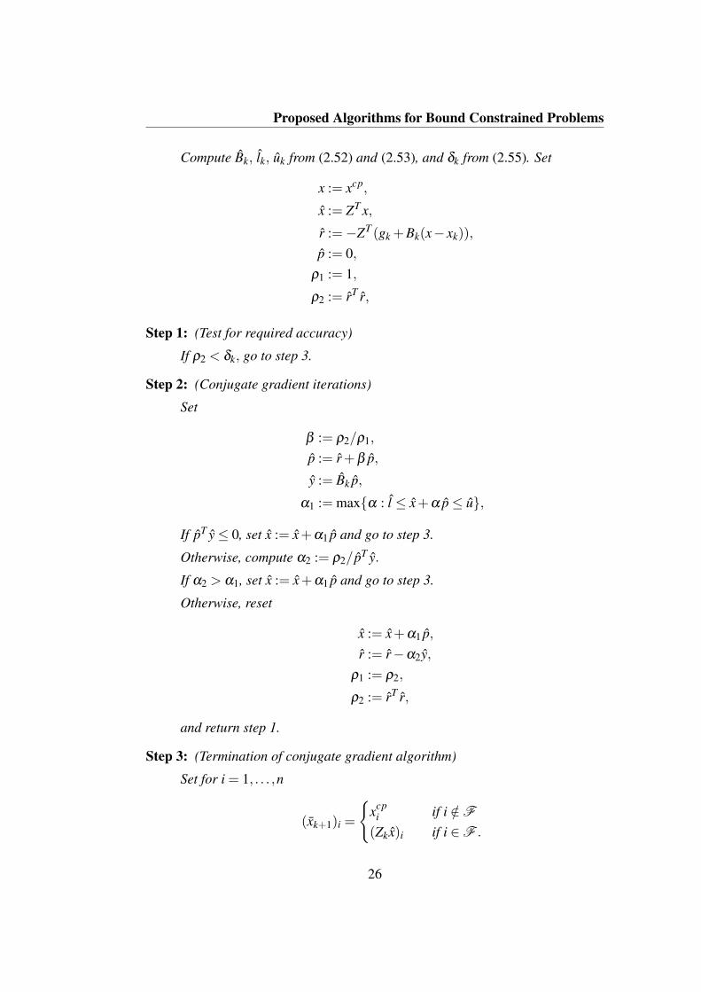
Algorithm 2.5.2. Cunjugate Gradient Method

Step 0: (Initialization.)

25


Compute Bk, lk, uk from (2.52) and (2.53), and δk from (2.55). Set

x := xcp,

x := ZT x,

r :=−ZT (gk +Bk(x− xk)),

p := 0,ρ1 := 1,

ρ2 := rT r,

Step 1: (Test for required accuracy)

If ρ2 < δk, go to step 3.

Step 2: (Conjugate gradient iterations)

Set

β := ρ2/ρ1,

p := r+β p,

y := Bk p,

α1 := max{α : l ≤ x+α p≤ u},

If pT y≤ 0, set x := x+α1 p and go to step 3.

Otherwise, compute α2 := ρ2/pT y.

If α2 > α1, set x := x+α1 p and go to step 3.

Otherwise, reset

x := x+α1 p,r := r−α2y,

ρ1 := ρ2,

ρ2 := rT r,

and return step 1.

Step 3: (Termination of conjugate gradient algorithm)

Set for i = 1, . . . ,n

(xk+1)i =

{xcp

i if i /∈F

(Zkx)i if i ∈F .

26


2.5.4 The AlgorithmIn this subsection, we summarize the method, which we have described in 2.5.1, inan algorithm. Before that we give some explanations about the approximated Hes-sian matrix Bk. We should mention that for global convergence of the algorithm,it is required that the Hessian approximations satisfy the following condition

∞

∑k=0

1/(1+ min0≤i≤k

‖Bi‖) = ∞

The above condition is satisfied if, for example, we have

‖Bk‖ ≤ λ1 + kλ2 (2.56)

for k ∈ N and fixed positive numbers λ1 and λ2.

The Hessian matrix can be approximated at each iteration by a number ofdifferent methods including BFGS,

Bk+1 = Bk +ykyT

kyT

k sk−

BksksTk Bk

sTk Bksk

,

and DFP,

Bk+1 = Bk +rkyT

k + ykrTk

yTk sk

−rT

k skykyTk

(yTk sk)2 ,

updating strategies. Where sk and yk represent, respectively, the displacementxk+1− xk and the change of the gradient gk+1−gk, and rk defined by

rk := yk−Bksk.

In both of the cases, we update only if the new approximation Bk+1 is guaranteedto be positive definite, more precisely, the updates are performed provided sk, yksatisfy the following condition

yTk sk

yTk yk≥ 10−8.

It has been shown in [15] that for the case of convex problems, the BFGS updatesremain uniformly bounded, therefore, the condition (2.56) is automatically sat-isfied in this case. Another method for approximating the Hessian matrix is thesymmetric rank-one(SR1) method which has the following update formula

Bk+1 = Bk +rkrT

krT

k sk,

27


This method does not guarantee that the new approximation is positive definiteand must be controlled so that the condition (2.56) holds. Moreover, we skip theupdate whenever the condition

‖rkrT

krT

k sk‖> 108

holds for the rank-one correction.

Now we are in the position, in which we can specify the algorithm.

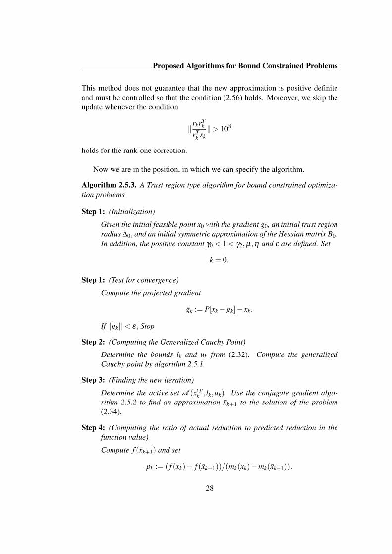
Algorithm 2.5.3. A Trust region type algorithm for bound constrained optimiza-tion problems


Given the initial feasible point x0 with the gradient g0, an initial trust regionradius ∆0, and an initial symmetric approximation of the Hessian matrix B0.In addition, the positive constant γ0 < 1 < γ2,µ,η and ε are defined. Set

k = 0.

Step 1: (Test for convergence)

Compute the projected gradient

gk := P[xk−gk]− xk.

If ‖gk‖< ε, Stop

Step 2: (Computing the Generalized Cauchy Point)

Determine the bounds lk and uk from (2.32). Compute the generalizedCauchy point by algorithm 2.5.1.

Step 3: (Finding the new iteration)

Determine the active set A (xcpk , lk,uk). Use the conjugate gradient algo-

rithm 2.5.2 to find an approximation xk+1 to the solution of the problem(2.34).

Step 4: (Computing the ratio of actual reduction to predicted reduction in thefunction value)

Compute f (xk+1) and set

ρk := ( f (xk)− f (xk+1))/(mk(xk)−mk(xk+1)).

28

2.6 L-BFGS-B

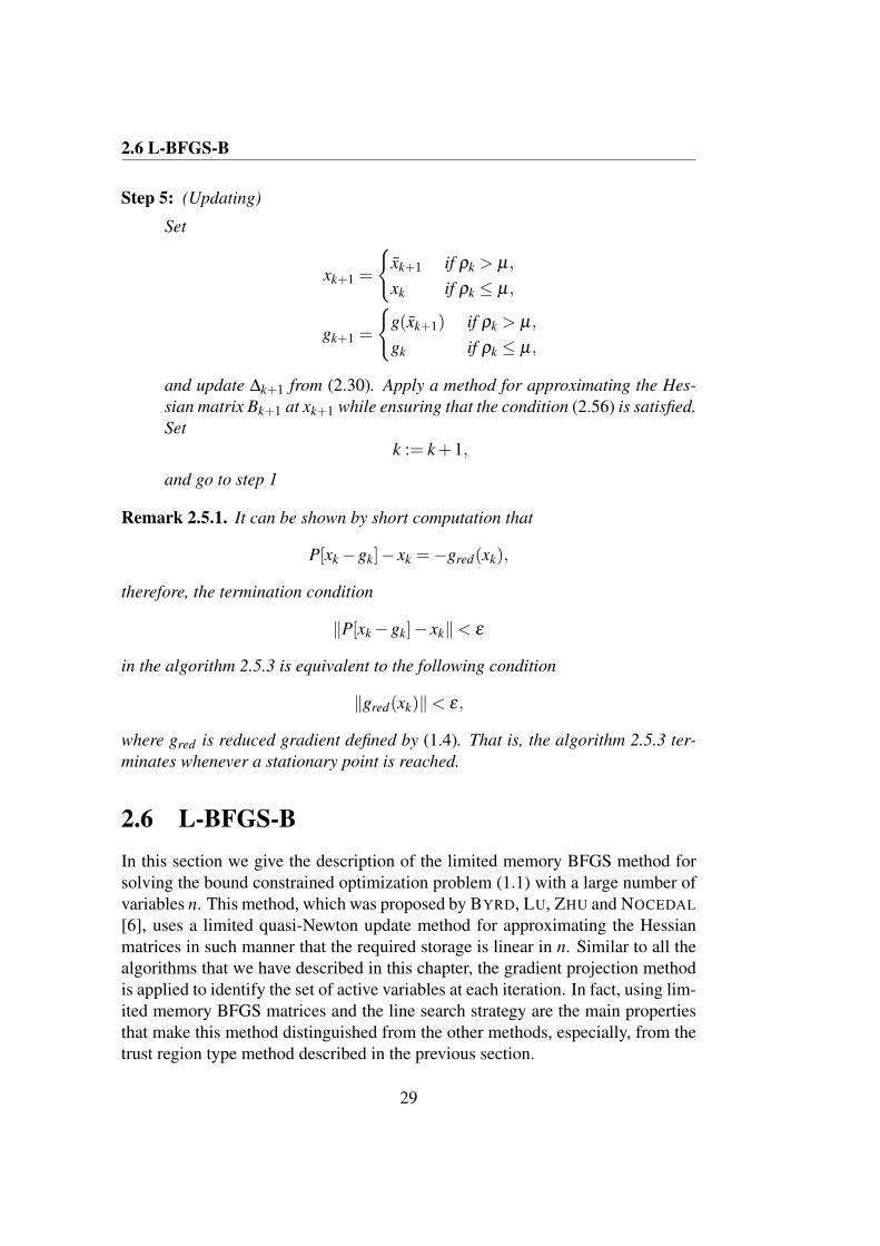
Step 5: (Updating)

Set

xk+1 =

{xk+1 if ρk > µ,

xk if ρk ≤ µ,

gk+1 =

{g(xk+1) if ρk > µ,

gk if ρk ≤ µ,

and update ∆k+1 from (2.30). Apply a method for approximating the Hes-sian matrix Bk+1 at xk+1 while ensuring that the condition (2.56) is satisfied.Set

k := k+1,

and go to step 1

Remark 2.5.1. It can be shown by short computation that

P[xk−gk]− xk =−gred(xk),

therefore, the termination condition

‖P[xk−gk]− xk‖< ε

in the algorithm 2.5.3 is equivalent to the following condition

‖gred(xk)‖< ε,

where gred is reduced gradient defined by (1.4). That is, the algorithm 2.5.3 ter-minates whenever a stationary point is reached.

2.6 L-BFGS-BIn this section we give the description of the limited memory BFGS method forsolving the bound constrained optimization problem (1.1) with a large number ofvariables n. This method, which was proposed by BYRD, LU, ZHU and NOCEDAL

[6], uses a limited quasi-Newton update method for approximating the Hessianmatrices in such manner that the required storage is linear in n. Similar to all thealgorithms that we have described in this chapter, the gradient projection methodis applied to identify the set of active variables at each iteration. In fact, using lim-ited memory BFGS matrices and the line search strategy are the main propertiesthat make this method distinguished from the other methods, especially, from thetrust region type method described in the previous section.

29


2.6.1 Outline of the AlgorithmSimilar to 2.5 at each iteration k with the iterate xk, we approximate the objectivefunction f with a quadratic model of the form

mk(x) = f (xk)+gTk (x− xk)

T Bk(x− xk), (2.57)

where gk is the gradient of objective function at xk, Bk is a positive definite matrixcomputed by the limited memory BFGS method. Then the quadratic model mk isapproximately minimized with respect to the feasible region {x ∈Rn : l ≤ x≤ u}.This task is done by, first, applying the gradient projection method to fix somevariables in one of their bounds and then minimizing the quadratic model over thesubspace of free variables.

The gradient projection method is performed by first considering the piece-wise linear path

xk(t) = P[xk− tgk, l,u],

which is obtained by projecting the steepest descent direction onto the feasibleregion, where the projection P[, , ] is computed from (2.5.1). Then we find thegeneralized Cauchy point xcp as the first local minimizer the piece-wise quadraticunivariate function

qk(t) = mk(xk(t)).

After xcpk has been computed, the values of variables whose index belongs to

A (xcpk ) = A (xcp

k , l,u) are held fixed. Then we solve approximately the followingquadratic programming over the subspace of free variables

minimize mk(x)subject to li ≤ xi ≤ ui, i /∈A (xcp

k ),xi = (xcp

k )i, i ∈A (xcpk ),

(2.58)

where A (xcpk , l,u), is defined as the set of indices corresponding to the variables

whose value at xcp is at one of their bounds. To solve (2.58), first we ignore thebound constraints and minimize the quadratic model mk(x) over the subspace offree variables, which can be done either by a direct method or an iterative methodwith respect to the subspace of free variables, or by a dual method in which theactive bounds are dealt by Lagrange multipliers. Then the path toward the solutionis truncated in such a way that the condition

li ≤ xi ≤ ui, i /∈A (xcpk ) (2.59)

is fulfilled.

30

2.6 L-BFGS-B

After the approximated solution xk+1 of (2.58) has been obtained, the newiterate xk+1 is computed by a line search strategy which enforces the strong Wolfeconditions along the descent direction Pk := xk+1− xk. That is, the new iterate iscomputed by

xk+1 = xk +αk pk (2.60)

where αk is a step-length that satisfies in the sufficient decrease condition

f (xk+1)≤ f (xk)+ γ1αkgTk pk, (2.61)

and the curvature condition

|gTk+1 pk| ≤ γ2|gT

k pk|, (2.62)

where γ1 < γ2 < 1 are fixed positive numbers. Now it remains to show that thedirection pk is a descent direction. Firstly, since the generalized Cauchy point xcp

is the minimizer of the quadratic model mk along the projected steepest descentdirection, we have

mk(xk)> mk(xcp),

unless the projected gradient is equal to zero. Moreover, xk+1 lies on a path fromxcp to the point that minimizes the quadratic model mk over the subspace of freevariables. Hence, the value of the quadratic model mk decreases along this path,in particular, mk(xk+1) can not be greater than mk(xcp) and we have

f (xk) = mk(xk)> mk(xcp)≥ mk(xk+1) = f (xk)+gTk pk +

12

pTk Bk pk,

which implies that

gTk pk +

12

pTk Bk pk < 0.

Since in this algorithm at each iteration, the limited memory BFGS method is usedto approximate the Hessian matrix, Bk is positive definite. Consequently, we have

gTk pk < 0.

2.6.2 Limited Memory BFGS UpdateIn this section we describe a method in which computing the limited memoryBFGS can be done efficiently. BYRD, NOCEDAL and SCHNABEL [7] have de-rived the compact representation form of the BFGS method which allows us toimplement the limited memory BFGS method efficiently.

31


Suppose that we are at the iterate xk, and the pair correcter vectors {si,yi} fori = 0, . . . ,k−1 are defined by

si =: xi+1− xi, yi := gi+1−gi, (2.63)

and also for i = 0, . . . ,k−1 the curvature condition

sTi yi > 0 (2.64)

is satisfied. Then the new BFGS matrix is computed by formula

Bk+1 = Bk−BksksT

k Bk

sTk Bksk

+ykyT

kyT

k sk. (2.65)

Now we have the following theorem [7, p, 6]

Theorem 2.6.1 (Compact Representation Of BFGS). Let B0 be symmetric andpositive definite and k pairs {si,yi}k−1

i=0 satisfy the curvature condition (2.64).Moreover, assume that k times update are applied to B0 by using pairs vectors{si,yi}k−1

i=0 and the direct BFGS formula (2.65), then the symmetric positive defi-nite matrix Bk can be expressed as

Bk = B0−[B0Sk Yk

][STk B0Sk CkCT

k −Dk

]−1[STk B0Y T

k

](2.66)

Where Ck ∈ Rk×k and diagonal matrix Dk ∈ Rk×k are defined by

(Ck)i, j :=

{sT

i−1y j−1 if i > j0 otherwise,

(2.67)

Dk :=diag [sT0 y0, . . . ,sT

k−1yk−1], (2.68)

and the correction matrices Sk,Yk ∈ Rn×k have the form

Sk := [s0, . . . ,sk−1], Yk = [y0, . . . ,yk−1]. (2.69)

Now we can use the update procedure, which is described in the above the-orem, to compute the limited memory BFGS matrices. In the case of limitedmemory BFGS, at each iteration we store a small number r of recent correctionpairs {si,yi} in the correction matrices Sk and Yk. This matrices are updated byremoving the oldest pair and adding the new pair to them. That is, the correctionmatrices belong to Rn×r and have the forms

Sk := [sk−r, . . . ,sk−1], Yk := [yk−r, . . . ,yk−1]. (2.70)

32

2.6 L-BFGS-B

Moreover, we choose B(k)0 = ωkI as the initial matrix where ωk is a positive scaler

computed by

ωk :=yT

k−1yk−1

sTk−1yk−1

. (2.71)

Now if the curvature condition (2.64) holds for correction pairs {si,yi} with i =k− r, . . . ,k− 1, then the limited memory BFGS matrix Bk which is computedby applying r times updates to the initial matrix ωkI, using the correction pairs{si,yi}k−1

k−r and the BFGS formula can be expressed as

Bk = ωkI−UkNkUTk (2.72)

where

Uk :=[Yk ωkSk

], (2.73)

Nk :=[−Dk CT

kCk ωkST

k Sk

]−1

, (2.74)

and Ck and Dk belong to Rr×r and defined as

(Ck)i, j :=

{sT

k−r−1+iyk−r−1+ j if i > j0 otherwise,

(2.75)

Dk :=diag [sTk−ryk−r, . . . ,sT

k−1yk−1]. (2.76)

It should be mentioned that the matrix Nk is a 2r×2r matrix and since the positiveinteger r is chosen to be small, the computation of N−1

k is cheap. Furthermore,throughout the algorithm we do not compute Bk explicitly.

It has been shown in [7] that similar to (2.72), the inverse limited memoryBFGS matrix Hk can be represented by

Hk =1

ωkI−UkNkUT

k , (2.77)

where

Uk :=[

1ωk

Yk Sk

], (2.78)

Nk :=

[0 −Q−1

k−Q−T

k Q−Tk (Dk +

1ωk

Y Tk Yk)Q−1

k

], (2.79)

33


and Qk ∈ Rr×r defined as

(Qk)i, j :=

{sT

k−r−1+iyk−r−1+ j if i≤ j0 otherwise.

(2.80)

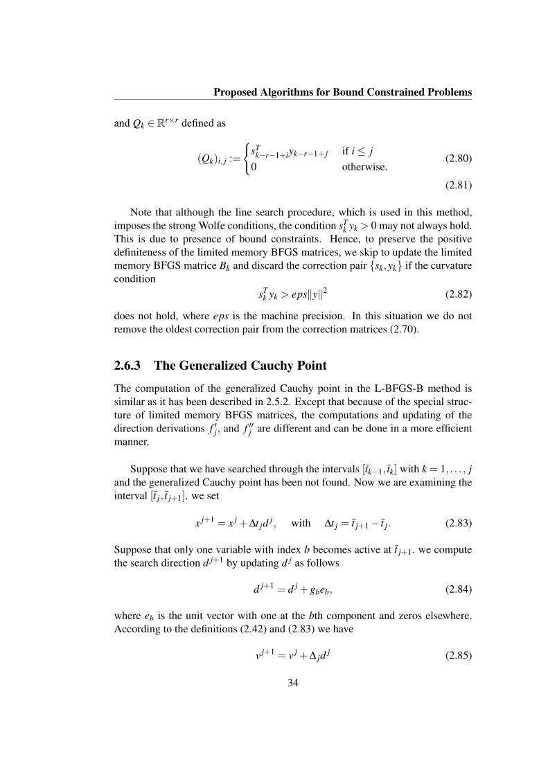
(2.81)

Note that although the line search procedure, which is used in this method,imposes the strong Wolfe conditions, the condition sT

k yk > 0 may not always hold.This is due to presence of bound constraints. Hence, to preserve the positivedefiniteness of the limited memory BFGS matrices, we skip to update the limitedmemory BFGS matrice Bk and discard the correction pair {sk,yk} if the curvaturecondition

sTk yk > eps‖y‖2 (2.82)

does not hold, where eps is the machine precision. In this situation we do notremove the oldest correction pair from the correction matrices (2.70).

2.6.3 The Generalized Cauchy Point

The computation of the generalized Cauchy point in the L-BFGS-B method issimilar as it has been described in 2.5.2. Except that because of the special struc-ture of limited memory BFGS matrices, the computations and updating of thedirection derivations f ′j, and f ′′j are different and can be done in a more efficientmanner.

Suppose that we have searched through the intervals [tk−1, tk] with k = 1, . . . , jand the generalized Cauchy point has been not found. Now we are examining theinterval [t j, t j+1]. we set

x j+1 = x j +∆t jd j, with ∆t j = t j+1− t j. (2.83)

Suppose that only one variable with index b becomes active at t j+1. we computethe search direction d j+1 by updating d j as follows

d j+1 = d j +gbeb, (2.84)

where eb is the unit vector with one at the bth component and zeros elsewhere.According to the definitions (2.42) and (2.83) we have

v j+1 = v j +∆ jd j (2.85)

34

2.6 L-BFGS-B

Hence by using (2.44), (2.45), (2.84) and (2.85) we have

f ′j+1 =gT d j+1 +(d j+1)T Bv j+1

=gT d j +g2b +(d j)T Bv j +∆t j(d j)T Bd j +gbeT

b v j+1

= f ′j +∆t j f ′′j +gTb +gbeT

b Bv j+1

(2.86)

and

f ′′j+1 =(d j+1)T Bd j+1

=(d j)Bd j +2gbeTb Bd j +g2

beTb Beb

= f ′′j +2gbeTb Bd j +g2

beTb Beb.

(2.87)

Note that since B is a dense matrix, the only expensive computations in (2.86) and(2.87) are

eTb Bv j+1, eT

b Bd j, and eTb Beb,

which can be accomplished in order O(n) operations . Nevertheless, by using thelimited memory BFGS formula

B = ωI +UNUT , (2.88)

and the definition (2.40), we can express the updating formula (2.86) and (2.87)as

f ′j+1 = f ′j +∆t j f ′′j +g2b +ωgbv j+1

b −gbUTb:NUT u j+1, (2.89)

f ′′j+1 = f ′′j −2ωg2b−2gbUT

b:NUT d j +ωg2b−g2

bUTb:Nub, (2.90)

where UTb: represents the bth row of the matrix U . Note that in (2.89) and (2.90)

only the computations of UT v j and UT d j require O(n) operations. However, be-cause from (2.84) and (2.85), the vectors v j+1 and d j+1 can be updated at eachiteration by simple computation, we can accomplished these computations in or-der O(r2) operations for a small integer r, provided we maintain the following2r-vectors at each iteration

q j+1 :=UT d j+1 =UT (d j +gbeb) = q j +gbub,

w j+1 :=UT v j+1 =UT (v j +∆t jd j) = w j +∆t jq j.

By using q j+1 and w j+1, we can express the directional derivatives f ′j+1 and f ′′j+as

f ′j+1 = f ′j +∆t j f ′′j +g2b +ωgbv j+1

b −gbUTb:Nw j+1,

f ′′j+1 = f ′′j −ωg2b−2gbUT

b:Nq j−g2bUT

b:NUb:.

35


If more than one variables will be active at t j+1 the above process, which outlinedabove, will be repeated again.

Now we are in the position that we can specify an algorithm for computing CPpoint:

Algorithm 2.6.1. Generalized Cauchy Point


Given x, l,u,g, and B = ωI +UNUT , for i = 1, . . . ,n compute the breakpoints and the components of the direction d in each coordinate by

ti :=

xi−ui

giif gi < 0

xi−ligi

if gi > 0

∞ otherwise,

di :=

{0 if ti = 0−gi otherwise

Initialize

F := {i : ti > 0}, (The set of indices corresponding to the free variables)

q :=UT d,w := 0,t := min

i∈Fti, (using the heapsort algorithm)

told := 0,∆t := t− told = t−0,b := i such that ti = t. Remove the b from F .

step 1: (Examining the first interval [0, t1])

Compute

f ′ := gT d =−dT d,

f ′′ := ωdT d−dTUNUT d =−ω f ′−qT nq∆tmin :=− f ′/ f ′′.

If ∆tmin < ∆t go to Step 4.

36

2.6 L-BFGS-B

Step 2: (examining the subsequent segments)

Set

xcpr :=

{ub if db > 0lb if db < 0.

Compute

vb := xcpb − xb,

w := w+∆tq,

f ′ := f ′+∆t j f ′′+g2b +ωgbvb−gbUT

b:Nw,

f ′′ := f ′′−ωg2b−2gbUT

b:Nq−g2bUT

b:NUb:.

q := q+gbUb:

Set

db := 0,∆tmin :=− f ′/ f ′′,

told := t,t := min

i∈Fti,

∆t := t− told,

b := i such that ti = t. Remove the b from F .

Step 3: (Loop)

If ∆tmin ≥ ∆t go to step 2.

Step 4: Set

∆tmin := max(∆tmin,0),told := told +∆tmin,

xcpi := xi + tolddi, for all i such that ti ≥ t,

For all i ∈F with ti = t, remove i from F .

w := w+∆tminq

Note that at last step of the above algorithm, the vector w is updated so that atthe termination we have

w =UT (xcp− xk). (2.91)

we will use this vector in the primal direct and the conjugate gradient method.

37


2.6.4 Subspace MinimizationAfter the generalized Cauchy point xcp has been determined, we deal with approx-imating the solution of (2.58) which consists of minimizing the quadratic modelmk over the subspace of free variables, and enforcing the bound constraints on thefree variables. In this section we shall present three methods including a directedprimal method, a conjugate gradient method which is similar to 2.5.3 and a dualmethod. In all of the three methods, first, we disregard the bound constraints andsolve the unconstrained problem with objective function mk over the subspace offree variables. Then the path obtained by the solution of unconstrained problemis truncated so that the bound constrained conditions are satisfied.

From now on, we denote the index set corresponding to the free variables atxcp by F , which can express alternatively as

Fk = {1,2, . . . ,n}\A (xcpk ),

where the subscript k stands for the outer iteration. Moreover, we define Zk to bea matrix with unit columns which span the subspace of free variables.

A Directed Primal MethodIn the directed primal method, the variables in which the generalized Cauchy pointlies at the bound remain fixed and we minimize mk over the subspace of freevariables by starting from xcp and enforcing the bound constraints correspondingto F . Hence, we consider only points x ∈ Rn of the form

x = xcp +Zk p,

where vector p belongs to the subspace of free variables. Now we can rewrite thequadratic model mk(x) as

mk(x) = f (xk)+gTk (x− xcp + xcp− xk)+

12(x− xcp + xcp− xk)

T Bk(x− xcp + xcp− xk)

= (gk +Bk(xcp− xk))T (x− xcp)+

12(x− xcp)T Bk(x− xcp)+ζ

:= pT rk +12

pT Bk p+ζ ,

where ζ is a constant,Bk := ZT

k BkZk (2.92)

is the reduced Hessian matrix, and

rk := ZTk (gk +Bk(xcp− xk))

38

2.6 L-BFGS-B

represents the projected gradient of the mk at xk onto the subspace of free variables.By using (2.91) and (2.72) the projected gradient rk can be rewritten as

rk = ZTk (gk +ωk(xcp− xk)−UkNkw), (2.93)

where the vector w has been already computed while computing the generalizedCauchy point. Now we can transform (2.58) to the following problem

minimize mk(p) :=12

pT Bk p+ rTk p (2.94)

subject to li− xcpi ≤ pi ≤ ui− xcp

i , i ∈Fk. (2.95)

As we have mentioned to solve the above problem, we ignore the bound con-straints (2.95) and solve the unconstrained problem (2.94), which is done by

pu :=−B−1k rk. (2.96)

Since the limited memory BFGS matrix Bk is a small-rank correction of a diag-onal matrix, for computing B−1

k we can apply the Sherman-Morrison-Woodburyformula, In particular, by using (2.72) we can express the reduced Hessian matrixB as

B = ωI−ZTU(NUT Z),

where the subscript k of the outer iteration is dropped for simplicity. By usingSherman-Morrison-Woodbury formula we obtain

B−1 =1ω

I +1ω

ZTU(I− 1ω

NUT ZZTU)−1NUT Z1ω.

By substituting above expression in (2.96), the solution of unconstrained problemcan computed by

pu =1ω

r+1

ω2 ZTU(I− 1ω

NUT ZZTU)−1NUT Zr. (2.97)

Once the Newton direction pu has been computed, we impose the bound con-straints (2.95) which is done by setting

p∗ := α∗pu, (2.98)

where the positive number α∗ is defined by

α∗ = max{α : α ≤ 1, li− xcp

i ≤ α pui ≤ ui− xcp

i , i ∈F}. (2.99)

Thus, we can express the approximated solution x of (2.58) as

xi =

{xcp

i if i /∈F

xcpi +(Zk p∗)i if i ∈F .

(2.100)

39


Algorithm 2.6.2. (Direct Primal method)Given x, l,u,g,w and B = ωI+UNUT .(Note that the subscript k for the outer

iteration have been omitted for simplicity)

Step 1: (Computing NUT Zr)

Compute

Zr := ZZT (g+ω(xcp− x)−UNw)

v :=UT Zrv := Nv

Step 2: (Computing M := I− 1ω

NUT ZZTU)

Set

M :=1ω

NUT ZZTU

M := I−NM

Step 3: (Computing the Newton direction pu)

Compute

v := M−1v

pu :=−( 1ω

r+1

ω2 ZTUv)

Step 4: (Imposing the bound constraints (2.95))

Compute

α∗ := max{α : α ≤ 1, li− xcp

i ≤ α pui ≤ ui− xcp

i , i ∈F}p∗ := α

∗pu

xi :=

{xcp

i if i /∈F

xcpi +(Zk p∗)i if i ∈F .

A Primal Conjugate Gradient Type MethodAnother approach for approximating the solution of (2.58) is to solve the positivedefinite linear system

Bk pu =−r, (2.101)

iteratively, by applying the conjugate gradient method. Similar to 2.5.3 the algo-rithm terminates whenever one the following conditions is satisfied:

40

2.6 L-BFGS-B

• One or more of the bound constraints (2.95) is violated.

• The residual in the conjugate gradient method is smaller than

δk := min(0.1,√||rk||)||rk||. (2.102)

It should be mentioned that since the limited memory BFGS matrix Bk is positivedefinite and also all of its eigenvalues are almost identical, it is suitable to use theconjugate gradient method.

Algorithm 2.6.3. (Conjugate Gradient Method)Given x, l,u,g,w,B = ωI+UNUT ,and δ from (2.102).(Note that the subscript

k of the outer iteration have been omitted for simplicity)

Step 0: (Initialization.)

Set

d := 0,

r := ZT (g+ω(xcp− x)−UNw),p :−r,

ρ1 := 1,

ρ2 := rT r,

Step 1: (Test for required accuracy)

If ρ2 < δ 2, go to step 3.

Step 2: (Conjugate gradient iterations)

Set

β := ρ2/ρ1,

p :=−r+β p,

y := Bp,α1 := max{α : li ≤ xcp

i +di +α pi ≤ ui},α2 := ρ2/pT y.

If α2 > α1, set d := d +α1 p and go to step 3.

Otherwise, reset

d := d +α1 p,r := r+α2y,

ρ1 := ρ2,

ρ2 := rT r,

and return step 1.

41


Step 3: (Termination of conjugate gradient algorithm)

Set for i = 1, . . . ,n

(xk+1)i :=

{xcp

i if i /∈F

xcpi +(Zkd)i if i ∈F .

A Dual MethodIn practice, it is usually observed that the number of active variables is small incomparison to the dimension of the problem. Thus, it should be appropriate to dealwith active bounds by corresponding Lagrange multipliers. This kind of methodsis referred to as a dual method. We consider the point x ∈ Rn of form

x := xk + p,

where xk + p is restricted to lie on the subspace of free variables at xcp. Which isdone by enforcing the condition

LTk p = LT

k (xcp− xk), (2.103)

where Lk is a matrix whose columns are unit vectors which constitute a basis forthe subspace of active variables at xcp. In addition, we have

LTk Zk = 0, LkLT

k +ZkZTk = I.

Now by stettingbk := LT

k (xcp− xk),

we form the following subspace problem

minimize gTk p+

12

pT Bk p (2.104)

subject to LTk p = bk (2.105)

l ≤ xk + p≤ u. (2.106)

Similar to other approaches in this section first we solve this problem withoutconsidering the bound constraints (2.106). This is done by writing the optimalityconditions

gk +Bk p∗+Lkµ∗ = 0, (2.107)

LTk p∗ = bk. (2.108)

42

2.6 L-BFGS-B

for (2.104)-(2.105), and multiplying (2.107) by LTk Hk from the right-hand-side,

where Hk represents the inverse of Bk. This yields

LTk Hkgk +LT

k P∗+LTk HkLkµ

∗ = 0,

by using (2.108) we obtain

(LTk HkLk)µ

∗ =−LTk Hkgk−bk. (2.109)

Since Lk is a full rank matrix and whose columns are unit vectors, LTk HkLT

k isa principal sub-matrix of Hk. Hence we can determine µ∗ by solving (2.109).Furthermore, since Hk is limited memory BFGS matrix and LT

k Lk = I, we canagain use the Sherman-Morrison-Woodbury formula to solve the linear system(2.109). To see this, we have

LTk HkLk =

1ωk

I +(LTk Uk)(NkUT

k LK).

By using the Sherman-Morrison-Woodbury formula we obtain

(LTk HkLk)

−1 = ωKI−ωkLTk Uk(I +ωkNkUT

k LkLTk Uk)

−1NkUTk Lkωk. (2.110)

Once µ∗ has been determined, we compute p∗ by solving the linear system

Bk p∗ =−Lkµ∗−gk. (2.111)

Finally, the approximated solution x of (2.58) is computed by

x = xcp +α∗(xk + p∗− xcp), (2.112)

where the positive number α∗ is defined by

α∗ = max{α : li− xcp

i ≤ α((xk)i + p∗i − xcpi )≤ ui− xcp

i , i ∈F}. (2.113)

Algorithm 2.6.4. (Dual Method)Given x, l,u,g,w,H = 1

ωI + UNU .T and we define nA the number of active

variables at xcp, In other words,

nA = |A (xcp, l,u)|.

(Note that the subscript k of the outer iteration have been omitted for simplicity)

Step 1: If nA = 0, Compute

u := UT gu := Nu

p∗ :=− 1ω

g−Uu

and go to step 5

43


Step 2: (Computing the right-hand-side of (2.109))

Compute

b :=−LT (xcp− xk)

v := UT gv := Mu

q := LTUv

q :=− 1ω

LT g−q−b

Step 3: (Computing µ∗)

Resetu := UT Lq

Form M = (I +ωNUT LLTU) as follows

M := ωUT LLTUM := I + NM

Compute

u := M−1Nu

µ∗ := ω

2LTUuµ∗ :=−ωq+µ

∗

Step 4: (Computing p∗)

Compute

u := UT Lµ∗

u := Nu+ v

p∗ :=− 1ω(Lµ

∗+g)+Uu

Step 5: Compute

α∗ = max{α : li− xcp

i ≤ α((xk)i + p∗i − xcpi )≤ ui− xcp

i , i ∈F},

and setx = xcp +α

∗(xk + p∗− xcp)

44

2.6 L-BFGS-B

2.6.5 The Algorithm for L-BFGS-BNow, at this moment we can summarize the L-BFGS-B method in to an algorithm.Similar to 2.5.3 we use

‖P[xk−gk]− xk‖∞ < 10−5 (2.114)

as the termination condition.

Algorithm 2.6.5. (L-BFGS-B)


Choose an initial point x0, and an integer r to be the number of limited mem-ory corrections stored. Define the initial limited memory Hessian matrix B0to be identity. Set

k := 0

Step 1: (Test for convergence)

If the condition (2.114) is satisfied, stop

Step 2: (Computing the generalized Cauchy point)

Compute xcp by algorithm 2.6.1.

Step 3: (Computing the descent direction)

Use one of the methods described in 2.6.4, including the directed primalmethod, the conjugate gradient method or the dual method, to determinethe approximated solution xk+1 of (2.58). Then set

pk := xk+1− xk

Step 4: (Line search iteration)

Implement a line search iteration along the direction pk, with respect to thebound constraints, to determine the step length αk, and set

xk+1 = xk +αk pk

Note that the line search starts with the unit as the initial value and satisfiesthe strong Wolfe conditions (2.61) and (2.64) with γ1 = 10−4 and γ2 = 0.9.

Step 5: (Updating gradient)

Setgk+1 := ∇ f (xk+1)

45


Step 6: If yk and sk satisfy the condition (2.82) with eps = 2.2× 10−16, add thevectors yk and sk to the correction matrices Sk and Yk.

If both of the matrices Sk and Yk have more than r update columns, removethe oldest columns from both of them.

Step 7: (Updating limited memory BFGS)

Update STk Sk,Y T

k Yk,Ck and Qk, and set

ω =yT

k yk

yTk sk

.

Step 8: (Loop)

Resetk := k+1,

and go to step 1

46

Chapter 3

A New Quasi Newton Method forBound Constrained problems

3.1 IntroductionIn this chapter we introduce a new approach [24] to solve the bound constrainedproblem (1.1). Our proposed method is an active set method that uses a combi-nation of the steepest descent directions and quasi Newton directions to identifythe optimal active bound constraints. Once the optimal set of active variableshas been identified, these variables are fixed at their bounds and the problem isreduced to a smaller problem over the subspace of free variables. This reducedproblem is solved by performing the bent line search method along the quasi New-ton direction. Particularly, the quasi Newton direction is computed by help of thelimited memory symmetric rank-one matrix. As it is known the SR1 matrices arenot necessarily positive definite, consequently, the quasi-Newton direction neednot be a descent direction. In such a case, we regularize this direction so that itwill become a descent direction. The convergence theory of the algorithm is alsoprovided.

3.2 Bent line SearchesIn this subsection, we give a description of a line search approach for the case ofbound constrained optimization problems

minimize f (x)subject to l ≤ x≤ u

(3.1)

In general, a line search method generates a descent sequence of feasible pointswhich is constructed at each iterate xk by choosing a search direction pk satisfying

47

A New Quasi Newton Method for Bound Constrained problems

the descent conditiongT

k pk < 0, (3.2)

and a corresponding search path xk +α pk for α > 0. Then the positive parameterαk is chosen in such a way that xk+1 := xk +αk pk satisfies the condition

f (xk+1)< f (xk), (3.3)

where the positive parameter αk is referred to as step-length.

From now on throughout this chapter, we drop the subscript k of the outeriteration for simplicity. Therefore, x,g, and p represent xk,gk and pk, and we writex for xk+1. Given a current iterate x, we call a component xi and the correspondingindex i active if either xi = li or xi = ui. Otherwise, if xi ∈ (li,ui), we call the ithcomponent and its corresponding index nonactice or free. In the case of boundconstrained optimization problems, a search direction p must be also a feasibledirection at x in addition to satisfy the descent condition.

Definition 3.2.1. Given a feasible point x, we call the direction vector d feasibleat x if there exists a sufficiently small α > 0 such that x+αd is feasible.

The feasibility of p at x requires that

pi ≥ 0 if xi = li,pi ≤ 0 if xi = ui.

}(3.4)

If the gradient g = g(x) has a nonzero component gi at a nonactive index i, we canmove from xi along both of the directions ±gi while remaining within feasibleregion. Therefore the value of objective function is reduced by moving from xialong the direction −gi. However, if xi is active in one of their bounds, onlychanges xi in one direction is possible, since by moving from xi along the oppositedirection we would lose the feasibility. Therefore, for an active variable i theobjective function f decreases if we have

gi < 0 if xi = li,gi > 0 if xi = ui.

}(3.5)

In this case, we say the variable xi can be freed from its bound.

As we have mentioned in 1.2, at a local minimizer x of the bound constrainedoptimization problem (1.1), we have

gred(x) = 0, (3.6)

where gred is the reduced gradient.

48

3.2 Bent line Searches

Definition 3.2.2. For an arbitrary feasible point x of the bound constrained opti-mization problem (1.1), we call an active bound on xi strongly active if one of thefollowing conditions is satisfied.

1. gi > 0 and xi = li,

2. gi < 0 and xi = ui.

Consequently, an active bound called weakly active if it is not strongly active.

While creating a line search method for bound constrained optimization prob-lems, we face several difficulties. First of all, as we have mentioned, in additionto being a descent direction the search direction p must be also a feasible direc-tion. Moreover, the search path must be modified since linear search path mayleave the feasible region. To be more accurate, let p be a search direction andx+α p(α > 0) be the corresponding linear search path, then for an index i thebound constraint [li,ui] is violated, provided either pi > 0 and ui < ∞, or pi < 0and li >−∞. To overcome this difficulty, we define the following piecewise linearBent line search path

x(α) = P[x+α p, l,u], (3.7)

which is obtained by projecting the linear path x+α p(α > 0) onto the boundconstraints

{x ∈ Rn : l ≤ x≤ u},

where P[, , ] is a projection defined by

(P[x, l,u])i =


xi if li < xi < ui.

The bent line search path is linear on each interval [αi−1,αi] for i = 1, ...,m+ 1.Where

0 = α0 < α1 < · · ·< αm < αm+1 = ∞,

and the break points α1, . . . ,αm belong to the set

S :=

{ui− xi

pi: pi > 0

}∪

{li− xi

pi: pi < 0

}\{0,∞}. (3.8)

Proposition 3.2.1. Suppose p is a feasible direction at x for which the followingconditions hold

1. gTred p < 0,

49


2. pi = 0 if either xi = li, gi > 0 or xi = ui, gi < 0,

then for sufficiently small α > 0 the bent search path (3.7) is feasible, and also wehave f (x(α))< f (x).

Proof. Due to the definition of the reduced gradient and second condition, it caneasily be shown that

gi pi = (gred)i pi for all i = 1, . . . ,n.

Hence, we havegT p = gT

red p≤ 0.

Since p is a feasible direction, we have x(α)= x+α p and consequently f (x(α))=f (x+α p) = f (x)+αgT p+o(α) if α > 0 is sufficiently small.

There are many ways to construct a bent line search. According to our con-vergence theory we need only to impose the following conditions

B1 If S = /0 or α < minS, the line search is efficient.

B2 If α ≥minS, the condition

f (x(α))< f (x) (3.9)

is satisfied.

To implement the bent line search satisfying the above conditions. First, we de-termine the values of α for which each component reaches its bound along thechosen search direction p by

αi :=

{(ui− xi)/pi if pi > 0 and ui < ∞

(li− xi)/pi if pi < 0 and li >−∞(3.10)

Then we eliminate the duplicate values of αi from the set {α1, . . . , αn} and sortthe remaining elements in an increasing ordered sequence α1,α2, . . . so that

0 = α0 < α1 < · · ·< αm < ∞.

Then we start with the first trial value α = α j with j = m. If (3.9) holds weterminates the line search method and accept αm as the step length. Otherwise,we replace j by b j

2c iteratively until one of the following cases is occurred:

1. An index j > 0 is obtained, for which the condition

f (x(α j))< f (x)

is satisfied.

50

3.3 Overview of the Algorithm

2. j = 0

In the first case, we apply a bisection procedure on the index set to improve indexj until it is determined that there is no neighbouring breakpoint than has a smallerfunction value. Then the corresponding breakpoint α j is accepted as the steplength. In the second case, the breakpoint search failed. Therefore, we performan ordinary line search iteration by using an efficient line search method withα ∈ (0,α1). Note that while performing the bent line search method, the set ofactive variables is changed either by dropping some variables when pi 6= 0 forsome active components, or by adding atleast one variable when a break point isaccepted as a step length.

3.3 Overview of the AlgorithmIn the case of bound constrained optimization problems, the choice of the searchdirection is a crucial point for proving global convergence of algorithms. There-fore close attention should be devoted to that. As it is has been mentioned in 1.2,the zigzagging behaviour is the major cause that makes the algorithms inefficient.In this situation, algorithms are unable to identify the set of optimal active boundconstraints, therefore, they free and fix the same variable alternatively in a largenumber of successive iterations. Indeed, we have no full control over whether theBent line search fixes variables, because often the Bent line search is not able tofind a efficient step length α < minS, and consequently accepts a break point asthe step length. Therefore, it remains just one way to prevent the bad zigzaggingbehaviour which is to control the conditions under which the variable are freed.

In order to obtain the fast rate of locally convergence, we have to performlocally steps which are done by means of an efficient unconstrained optimizationmethod over the subspace of nonactive variables; but this is reasonable only if theresulting step is not bent. Therefore such a local step is performed whenever in theprevious step no variable has been fixed in one of its bounds. On the other hand, ifin the previous step a new variable was fixed in its bounds, it does not make senseto perform the local step as the set of active variables is likely to change again.In such a case we perform a standard step which is done by performing thebent line search iteration along the steepest descent direction over the subspace ofnonactive variables. The search direction p used in a standard step is negative ofthe scaled gradient direction in the subspace of nonactive variables, which consistsof components

pi =

{−digi if i ∈ I,0 otherwise ,

(3.11)

51


where di are positive scaling numbers of the order of square of typical change inthe ith component, and I consists of indices corresponding the variables whicheither are nonactive or can be freed, provided the previous step was a freeing step.In all other cases I consists only of indices corresponding nonactive variables.

Suppose that in the previous step no variable has been fixed in one of itsbounds, now we have to make a decision between performing a freeing step orlocal step. In order to prevent the zigzagging behaviour, first we perform a localstep. Then we check whether a new variable became active. If a variable has beenactive, we perform a standard step. After that, again we check whether a activevariable can be freed. If a variable can be free, we do a freeing step. Otherwise,we repeat the local step again.

while implementing the algorithm, We terminate the algorithm whenever oneof the following conditions are satisfied

1. The norm of reduced gradient (1.4) is sufficiently small.

2. A large number of iterations have been done.

Note that if the first condition is satisfied, the algorithm terminates at a station-ary point of problem and consequently the first optimality condition holds for thispoint.

In order to analyse the convergence of the algorithm, we need to considerinfinity many iterations. Thus, in the following idealized version of the algorithm,we only terminate the algorithm whenever the reduced gradient is zero.

Algorithm 3.3.1. (Proposed Algorithm)


Given a feasible initial point x0 with function value f 0 and gradient vectorg0. Set

I := {i : li < x0i < ui or (g0

red)i 6= 0}

Step 2: (Standard step)

If the reduced gradient is zero, Stop

Otherwise, if I = /0, go to step 4.

Otherwise, Perform the bent line search method along the standard direc-tion over the subspace of variables corresponding to I to compute the newx. Set

I := {i : li < xi < ui}.Then, if some bound have been fixed, repeat step 2

52

3.4 Convergence Analysis

Step 3: (Local step)

If reduced gradient is zero, stop

Otherwise, perform the bent line search method along the direction deter-mined by a quasi Newton method over the subspace of variables corre-sponding to I to compute new x. Set

I := {i : li < xi < ui}.

Then, if a new bound has been fixed, go to step 2.

If no variable can be freed, repeat step 3

Step 4: (Freeing step)

SetI := {i : li < xi < ui or (gred)i 6= 0},

and continue with step 2.

The initial point in the first step is either chosen by user, or is given by

x0i :=

{li if li > 0,ui if ui < 0,

as the absolutely smallest point x0 in the feasible region.

3.4 Convergence AnalysisIn this section, we derive the global convergence result for our method. To ensureglobal convergence, not only the step length must be well chosen but also thesearch direction must be well chosen. In particular, additional to be feasible, ananother requirement is imposed on the angle between the search direction and thesteepest descent direction.

Definition 3.4.1. let sk =: xk+1− xk be the step and pk be a descent search direc-tion, along which xk+1 is obtained by performing a line search method. We callthis line search method efficient if at each iteration, it produces a step such thatsatisfies the condition

inf0≤l≤k

( fl− fl+1)‖sl‖2

(gTl sl)2 > 0, (3.12)

53


where ‖.‖ is an arbitrary norm in Rn. Equivalently, a line search procedure isreferred to as efficient if there exists an ε > 0 such that for all steps 0≤ l ≤ k, wehave

fl+1 ≤ fl− εgT

l sl

‖sl‖2 .

Efficiency of the line search procedure is one of the key requirements whichis need to be satisfied in order to obtain global convergence of the algorithms in-volving the line search strategies.

In order to obtain the convergence result, it is required that the sequence ofiterations {xk}k to be bounded. This condition is satisfied whenever for someindex k the level set

{x ∈F : f (x)≤ f (xk)}is bounded, where F is the feasible region of (1.1) consisting of only bound con-straints. In most applications, this is satisfied for some iterates xk.

In the following convergence result, the degenerate stationary point is the onlycase in which the weakly active constraints might pop in and out of the active setin the zigzagging manner.

Theorem 3.4.1. Let f be continuously differentiable on the feasible region F .Assume that all search directions p are feasible and also satisfy

pi = 0 if either xi = li,gi > 0 or xi = ui,gi < 0, (3.13)

and the reduced angle condition

supgT

red(x)p‖gred(x)‖‖p‖

< 0. (3.14)

If the sequence of iteration points {xk}k is bounded then:

(i) The the reduced gradient gred(xk) satisfy

infk≥0‖gred(xk)‖= 0. (3.15)

(ii) If the algorithm does not terminate but xk→ x for k→ ∞, then x satisfies thefirst order optimality conditions gred(x) = 0, and for all i and sufficientlylarge k, we have

(xk)i = xi = li if gi(x)> 0,(xk)i = xi = ui if gi(x)< 0.

(3.16)

54

3.4 Convergence Analysis

Note that the condition (3.14) is automatically satisfied for the steepest descentdirection, consequently this condition always holds at the standard step.

Proof. Every thing is trivial when the algorithm terminates at a stationary point;therefore, we might assume that infinitely many iterations are done. W.l.o.g., wecan assume that li < ui for all i.

(i) Suppose that the line search is efficient only finitely often then there exists aninteger L such that for all iterations k > L, condition B1 is violated, and con-sequently the condition B2 is satisfied, in particular, the set of breakpointsis not empty, and atleast a new bound is fixed. Hence ultimately, at eachiteration some new bounds are fixed. But this means that ultimately, onlystep 2 is executed. Since the number of variables n is finite and no boundcan be freed in the step 2, this can happen only in a finite number of itera-tions. This is a contradiction with our assumption.

Therefore, the line search is infinitely often efficient, and by (3.4.1), thereexists a number δ > 0 such that infinitely often

( fk− fk+1‖sk‖2)

gTk sk

≥ δ . (3.17)

Now by (3.13) and definition of the reduced gradient, for each componenti ∈ {1, ...,n} we have one of the following cases

1. gred(xk)i = (gk)i,

2. gred(xk)i = 0≤ (gk)i and (xk)i = li,

3. gred(xk)i = 0≥ (gk)i and (xk)i = ui.

By (3.13) for the cases 2 and 3 we have

(xk+1)i− (xk)i = (sk)i = α(pk)i = 0.

Therefore for all cases, gred(xk)i(sk)i = (gk)isi, and by summing over alli ∈ {1, ...,n} we obtain

gTk sk = gT

red(xk)sk.

Since the sequence of iterations {xk}k is bounded and the objective functionf is continuous, the sequence fk := f (xk) is also bounded. Therefore f :=inf fk is finite. Moreover, Since we generate a descent sequence, we havelim fk = f . Hence, after infinitely many iterations satisfying (3.17), we have( writing −ε < 0 for the left hand side of (3.14))

ε‖gred(xk)‖≤−gT (xk)pk

‖pk‖=|gT

red(xk)pk|‖pk‖

=|gT

red(xk)sk|‖sk‖

≤√

fk− fk+1

δ→ 0,

55


as k→ ∞, and consequently we have

infk≥0‖gred(xk)‖= 0.

(ii) By continuity of the gradient, we have

g := g(x) = liml→∞

gk.

If i is an index for which gi > 0 and (xk)i = li, then there exists a numberL′′ such that (gk)i > 0 for k > L′′, analogously, there exist a number L′

such that (gk)i < 0 for all k > L′ provided gi < 0 and (xk)i = ui. Nowdue to the definition (1.4) of the reduced gradient we have for all iterationsk > L := max(L′,L′′),

(gred(xk))i =

0 if (xk)i = li,0 if (xk)i = ui,

(gk)i otherwise.

By part (i), there is a subsequence of gred(xk) which converges to zero.Now we show that the active variables (xk)i = li and (xk)i = ui remain fixedat their bounds for infinitely many iterations k > L. Since for each activevariable (xk)i = li

((xk)i = ui

)we have (gk)i > 0

((gk)i < 0

)for all k > L,

all active variables are strongly active. Therefore, they can not be freedanymore. This fact implies that (xk)i = li

((xk)i = ui) for all k > L, and

consequently, xi = limk→∞(xk)i = li(xi = limk→∞(xk)i = ui

). Therefore the

conditions (3.16) are satisfied.

From (3.16) and the definition of the reduced gradient, we conclude thatgred(x) = limgred(xk) = 0. Hence the first order optimality condition is sat-isfied.

3.5 Local StepIn this section we are dealing with computation of the search direction in the lo-cal step of the algorithm 3.3.1. As we have mentioned, in order to obtain fastlocally convergence we apply a limited quasi Newton method for unconstrainedoptimization problems in the local step. To be more accurate, suppose that while

56

3.5 Local Step

performing algorithm 3.3.1, no variable has been fixed after execution of the stan-dard step and also the feasible point x with I := {i : li < xi < ui} has been de-termined. Now in local step, the quasi Newton search direction is computed bysolving the following optimization problem

minimize pT Bp+gT p+ f (x)subject to pi = 0, i /∈ I,

(3.18)

where g is the gradient of f at feasible point x, and B is a limited memory SR1approximation of the Hessian matrix ∇2 f . Now the problem (3.18) can be trans-formed to the following unconstrained problem defined over the subspace of non-active variables corresponding to the set I

minp∈R|I|

pT Bp+ gT p, (3.19)

whereB := ZT BZ (3.20)

is the reduced Hessian matrix, and

g := ZT g (3.21)

represents the projection of the gradient vector g(x) onto the subspace of non-active variables corresponding to I, and Z is a matrix whose columns are unitvectors spanning the subspace of nonactive variables corresponding to I. As weknow from general theory of unconstrained optimization, the solution of (3.19) iscomputed by

p f :=−B−1g. (3.22)

Hence the solution of (3.18) is determined by

p f := Z p f . (3.23)

Since the matrix B is computed by the limited memory SR1 method, we haveno guarantee that the search direction p f is a descent direction. However, fromour convergence result, the search directions p f must satisfy the angle condition(3.14). In following we will explain, how this search direction is regularized inorder to satisfy the condition (3.14) in case it fails to hold for (3.23). First we givea description about updating the limited memory SR1 matrices.

3.5.1 Limited Memory SR1 UpdateSimilar to the BFGS matrices, the compact representation of SR1 matrices canbe derived. This compact representation introduced by BYRD, NOCEDAL and

57


SCHNABEL [7] is similar to ones developed for the BFGS formula, except thatunder some conditions it requires less storage. The SR1 matrices are updated ateach iteration k by the following update formula

Bk+1 = Bk +(yk−Bksk)(yk−Bksk)

T

(yk−Bksk)T sk, (3.24)

wheresk := xk+1− xk, yk := gk+1−gk.

It should be mentioned that the above update is well defined only if

(yk−Bksk)T sk 6= 0.

In our implementation it has been observed that, the SR1 method does not breakdown and performs well if the update is skipped whenever the denominator of(3.24) is small. In particular, the update formula (3.24) is applied whenever thefollowing condition

|(yk−Bksk)T sk| ≥ 10−8‖sk‖‖yk−Bksk‖ (3.25)

holds. Now we present the compact representation of SR1 matrices by means ofthe following theorem.

Theorem 3.5.1. (Compact Representation of SR1 [7, p, 20]) Suppose that thesymmetric matrix B0 is updated k times by the SR1 formula (3.24) using the pairs{si,yi}k−1

i=0 , and assume that each update is well defined. In another words, wehave (y j−B js j)

T s j 6= 0 for all j = 1, . . . ,k− 1. Then the symmetric SR1 matrixBk can be expressed as

Bk = B0 +(Yk−B0Sk)N−1k (Yk−B0Sk)

T , (3.26)

where the correction matrices Sk,Yk ∈ Rn×k have the form

Sk := [s0, . . . ,sk−1], Yk = [y0, . . . ,yk−1], (3.27)

the matrixNk := Dk +Ck +CT

k −STk B0Sk (3.28)

is nonsingular, Ck ∈ Rk×k and diagonal matrix Dk ∈ Rk×k are defined by

(Ck)i, j :=

{sT

i−1y j−1 if i > j0 otherwise,

(3.29)

Dk :=diag [sT0 y0, . . . ,sT

k−1yk−1]. (3.30)

58

3.5 Local Step

Similar to the limited memory BFGS method described in 2.6.2, we can de-velop the above update formula for the limited memory SR1 matrices. To see this,the initial matrix B0 is replaced with a basic matrix B0

k = ωkI at the kth iteration,where ωk is positive scaling number or can be computed by

ωk :=yT

k−1yk−1

sTk−1yk−1

. (3.31)

Moreover, in the case of limited memory the correction matrices Yk and Sk containonly the r most recent correction vectors

Sk := [sk−r, . . . ,sk−1], Yk := [yk−r, . . . ,yk−1], (3.32)

where r is a fixed integer number. At each iteration, these matrices are updatedby removing the oldest correction pair and inserting the new correction pair. Nowwe can express the limited memory SR1 matrices as follows:

Bk = ωkI +UkN−1k UT

k , (3.33)

where

Uk :=Yk−ωkSk, (3.34)

Nk :=Dk +Ck +CTk −ωkST

k Sk, (3.35)

Ck and Dk belong to Rr×r and are defined as

(Ck)i, j :=

{sT

k−r−1+iyk−r−1+ j if i > j0 otherwise,

(3.36)

Dk :=diag [sTk−ryk−r, . . . ,sT

k−1yk−1]. (3.37)

Note that the matrix Nk belongs to Rr×r, furthermore, the positive integer r ischosen to be small. Therefore, the computation of Nk is cheap at each iteration.

3.5.2 Computing the Search DirectionNow we are in the position that we can explain how the quasi Newton searchdirection is computed in order to satisfy the condition (3.14). As it has beenmentioned before the first quasi Newton direction is computed by solving thefollowing linear system

Bp =−g (3.38)

By using (3.33) and (3.20), we can rewrite the above linear system as

(ω I +UN−1UT )p =−g, (3.39)

59


where U := ZTU and I ∈ Rr×r is the identity matrix. Note that the subscriptionk of the outer iteration is eliminated for simplicity. Now by using (3.39) anddefining vector

h := N−1UT p, (3.40)

we havep =− 1

ωg− 1

ωUh. (3.41)

Furthermore, by substituting (3.41) in (3.40) we have

h = N−1UT (− 1ω

g− 1ω

Uh), (3.42)

where (3.42) is a linear system containing only an unknown vector h. By solvingthis linear system we have

h = (N +1ω

UTU)−1(− 1ω

UT g). (3.43)

Now we can define our search direction as a function of κ as follows

p(κ) =− 1ω

g−κq, (3.44)

whereq :=

1ω

Uh.

In our proposed method, first we set κ = 1 and test whether the condition

gT p(κ)‖g‖‖p(κ)‖

≤ −δ , (3.45)

is satisfied for a fixed positive number δ ∈ (0,1). If it is satisfied then p(1) isaccepted as the search direction in the local step. But if the above condition doesnot hold for κ = 1, we choose κ such that the condition (3.45) will be satisfied forchosen κ .

Now, it remains to show how κ is chosen in order to satisfy (3.45). By substi-tuting (3.44) into the condition (3.45) we have

− 1ω‖g‖2−κ gT q

‖g‖‖− 1ω

g−κq‖≤ −δ , (3.46)

and consequently

‖g‖ 1δ

( 1ω

+κgT q‖g‖

)≥ ‖− 1

ωg−κq‖. (3.47)

60

3.5 Local Step

Now by defining

τ :=1δ

( 1ω

+κgT q‖g‖2

), (3.48)

we can rewrite (3.47) as

‖g‖τ ≥ ‖ 1ω

g+κq‖. (3.49)

Since the both sides the above inequality are nonnegative, we can compute thesquares of them without switching the inequality direction as follows

‖g‖2τ

2 ≥ 1ω2‖g‖

2 +κ2‖q‖2 +

2κ

ωgT q. (3.50)

By computing κ from (3.48), we obtain

κ := (δτ− 1ω)‖g‖2

gT q(3.51)

By using (3.50) and (3.51) and eliminating ‖g‖2 from the both sides of the in-equality we have

τ2 ≥− 1

ω2 +2δτ

ω+(δτ− 1

ω)2‖g‖2‖q‖2

(gT q)2 . (3.52)

Now by adding −δ 2τ2 to the both sides of the above inequality we obtain

(1−δ2)τ2 ≥− 1

ω2 +2δτ

ω−δ

2τ

2 +(δτ− 1ω)2‖g‖2‖q‖2

(gT q)2 , (3.53)

which can be express as

(1−δ2)τ2 ≥ (δτ− 1

ω)2(‖g‖2‖q‖2

(gT q)2 −1), (3.54)

Since (1−δ 2) is positive we can rewrite (3.54) as

τ2

(δτ− 1ω)2≥(‖g‖2‖q‖2− (gT q)2

(1−δ 2)(gT q)2

), (3.55)

which implies thatτ

1ω−δτ

≥ ∆, (3.56)

where

∆ :=

√‖g‖2‖q‖2− (gT q)2

(1−δ 2)(gT q)2 . (3.57)

61


By using (3.56), we have

τ ≥ (1ω−δτ)∆,

⇔ τ(1+∆δ )≥ ∆

ω,

⇔ τ ≥ ∆

(1+∆δ )ω. (3.58)

By substituting (3.48) into (3.58), we obtain

1δ

( 1ω

+κgT q‖g‖2

)≥ ∆

(1+∆δ )ω, (3.59)

which yields

κgT q‖g‖2 ≥

δ∆

(1+δ∆)ω− 1

ω=

−1(1+δ∆)ω

, (3.60)

and consequently κ ≥

( −1(1+∆δ )ω

)‖g‖2

gT qif gT q > 0,

κ ≤( −1(1+∆δ )ω

)‖g‖2

gT qif gT q < 0.

(3.61)

In our proposed method, we choose

κ =( −1(1+∆δ )ω

)‖g‖2

gT q, (3.62)

where ∆ is computed from (3.57). After κ has been computed, we define thesearch direction as

p := Z p(κ) =−Z(1ω

g+κq) (3.63)

Now we can summarize the description outlined above into the following algo-rithm

Algorithm 3.5.1. (Local step)


Given ω,U,N, a fixed number δ ∈ (0,1) and the gradient g of the currentiterate x. Assume that the set of free variable I at x has been determined.

62

3.5 Local Step

Step 1: (Computing p = B−1g )

Set

θ :=1ω

g := ZT g

U := ZTU

T := N +θUTU

h :=−θUT gh := T\hq := θUhp :=−θ g−q

Step 3: (Testing the angle condition (3.45))

Set

ng := ‖g‖np := ‖ p‖

If gT pn png≤ δ , then go to step 4

Otherwise,set

η := gT qnq := ‖q‖

∆ :=

√n2

gn2q−η2

η2(1−δ 2)

κ :=( −θ

1+∆δ

)n2g

η

p :=−θ g−κq

Step 4: (Computing the search direction)

Setp := Z p

63

Chapter 4

Numerical Experiments

4.1 IntroductionIn this chapter, we test our proposed algorithm by solving a list of bound con-strained optimization problems. These problems are selected from CUTEr collec-tion [14] and most of them are large scale problems. Then, the performance of ouralgorithm is demonstrated for different choices of the limited memory parameterr. Finally, we compare the performance of our algorithm with L-BFGS-B.Throughout our implementations, we use

‖gred(x)‖∞ ≤ 10−5 (4.1)

as the termination condition. Moreover, while performing the bent line search ap-proach if the break point search fails, we perform the efficient line search by meansof the routine of MORE and THUENTE [23] which tries to impose the strong Wolfeconditions. After testing a small number of test problems, we have realized thatthe algorithm works well with the choice of δ = 0.01 for the most of problems,where δ is defined in the angle condition (3.14). All of codes have been writtenin MATLAB and we have used the new MATLAB interface of CUTEr testing en-vironment from http://www.cuter.rl.ac.uk/download.html.

4.2 Numerical ResultsFirst, we have tested our algorithm with different choices of the limited memoryparameter r which represents the number of stored correction pairs in the correc-tion matrices. Namely, we set r = 3, r = 5, r = 17 and r = 29. The correspondingnumerical results are represented by table 4.1, where the first column in this tablereveals the names of test problems, the second column represents the dimensions

64

http://www.cuter.rl.ac.uk/download.html

4.2 Numerical Results

n of the problems. We record the total run time Time, the number of functionevaluations n f e and the number of gradient evaluations nge for each test problem.

Problem n r = 3 r = 5 r = 17 r = 29Time nfe nge Time nfe nge Time nfe nge Time nfe nge

TORSION1 5476 1.962 2880 318 1.313 1933 207 2.225 2049 241 3.685 2062 242TORSION2 5476 1.884 2406 266 1.222 1711 196 2.034 1780 211 5.246 2786 342TORSION3 5476 1.221 1395 191 1.119 1590 230 1.206 1092 152 2.700 1487 212TORSION4 5476 1.144 1382 187 0.666 929 128 0.928 844 114 3.321 1807 267TORSION6 5476 0.610 638 97 0.377 501 70 0.611 514 74 0.643 446 66BDEXP 5000 0.081 2 2 0.015 2 2 0.005 2 2 0.010 2 2BQPGASIM 50 0.220 347 64 0.035 249 43 0.033 173 30 0.040 173 30JLBRNGA 10000 9.422 8158 853 6.703 5543 569 13.467 6354 671 35.113 10719 1217LINVERSE 1999 10.479 27162 3187 3.168 8334 810 5.040 9284 842 6.640 8395 740MCCORMCK 5000 0.408 221 41 0.364 273 80 0.326 184 34 0.308 168 32PROBPENL 500 0.436 5 3 0.026 5 3 0.004 5 3 0.002 5 3NONSCOMP 5000 0.151 8 4 0.025 8 4 0.019 8 4 0.006 8 4OBSTCLAE 10000 9.303 8095 657 4.668 3992 363 8.196 4261 370 13.395 4682 363OBSTCLAL 10000 3.728 3144 290 2.973 2569 237 3.647 1946 178 5.330 1821 174OBSTCLBL 10000 3.696 3016 258 3.611 3022 259 5.011 2663 218 7.445 2644 215OBSTCLBM 10000 3.265 2683 238 2.439 2036 174 4.721 2461 233 6.831 2350 218OBSTCLBU 10000 3.811 3197 287 3.696 3120 270 4.441 2372 207 5.655 2033 170

Table 4.1: Results of the algorithm 3.3 for various choices of the limited memory param-eter r

An important observation on the results in table 4.1 is that on these problemsin the case of r = 5 the algorithm works more efficient than in the other cases. Inother word, in the case of r = 5, the algorithm requires less time, function evalua-tions and gradient evaluations for the most of problems.

In order to analyse the result of table 4.1, we use the performance profileintroduced by DOLAN and MORE [11]. This performance profile is defined by

ρAlg(τ) =number of test problems for which log2(rP,Alg)≤ τ

number of all test problems, (4.2)

where τ ≥ 0, and rP,Alg is the performance ratio defined by

rP,Alg =the time required to solve problem P by algorithm Alg

the shortest time required to solve problem P. (4.3)

Note that, the performance ratio (4.2) can be computed with respect to an ar-bitrary performance measure, for instance, the number of function evaluations or

65


the number of gradient evaluations. Furthermore, if an algorithm Alg fails to solvea test problem P, the corresponding performance ratio rP,Alg is set to be infinity(or a large number).

The nondecreasing, piecewise constant function ρAlg : R→ [0,1] is the cu-mulative distribution function for performance ratio. In the performance profilesthe value of ρAlg(τ) at τ = 0 yields the percentage of the test problems for whichthe algorithm Alg is the best and the value of ρAlg(τ) for large enough values ofτ gives the percentage of the test problems that the algorithm Alg can solve. Inaddition, the value of ρAlg(τ) at τ = 1 gives the probability that the algorithm Algwill win over the rest of algorithms. Therefore, if the number of wins is of ourinterest, we need to compare the value of ρAlg(1) for all of the algorithms.

The figures 4.1 show the performance profile of the algorithm 3.3 based on thetable 4.1. These figures reveal the relatively performance of the algorithm for dif-ferent setting of the limited memory parameter r with respect to the performancemeasures including the number of objective function evaluations, the number ofgradient evaluations and the required time. Furthermore, the relative efficiencyof the algorithm in each case can be directly observed from the figures. In otherword, the higher is the particular curve, the better is the corresponding case forthe algorithm.

As we can see from the figure 4.1(b), in the case r = 5 the algorithm has themost wins, consequently, it has the highest probability for being the optimal solverwhen the computational time is compared. However as the figures 4.1(c) , 4.1(a)reveal, the performance of the algorithm is almost the same in all the cases whenthe number of function or gradient evaluations is compared. In the case of r = 3and r = 5 updating the Hessian matrix is cheaper than the other cases while inthese cases the algorithm needs more iterations to solve the problem in compari-son to the cases r = 17 and r = 29. Since in cases r = 19 and r = 29 the updatingHessian matrix require longer time in comparison to evaluation of the objectivefunction and gradient, the algorithm has the better performance in the case ofr = 5. Although in case r = 3, updating the Hessian matrix is cheaper than inthe rest of cases, the algorithm needs more iterations to reach the stationary point.This is due to the fact that in the case r = 3, the limited memory Hessian matrixis updated by using just the three most recent correction vectors at each iteration.Therefore, the limited memory Hessian matrix can not be good approximation forthe Hessian matrix and consequently the algorithm performs many iterations tosolve the problem.

In the next part of this chapter we compare the performance of our algorithm in

66


(a) Function evaluations

(b) Time

(c) Gradient evaluations

Figure 4.1: Performance profiles of the algorithm 3.3 based on the table 4.1

67


tow cases with L-BFGS-B method described in 2.6. The L-BFGS-B codes is writ-ten in MATLAB from [6]. The test functions are the same test function presentedin table 4.1. we test our algorithm with different bent line search approaches:

Alg 1: The bent line search used in the algorithm performs the bisection proce-dure to improve the index at each iteration.

Alg 2: The bent line search used in the algorithm does not perform the bisectionprocedure.

The figure 4.2 shows the performance profiles of our algorithm in comparisonto L-BFGS-B. As performance measures, we use number of objective functionevaluations (4.2(b)), number of gradient evaluations (4.2(c)), and required com-putational time (4.2(a)). In figure 4.2(a) we see that our algorithm in both ofcases dominates L-BFGS-B. This stems from the following facts: first, updatingthe limited memory SR-1 matrices is cheaper that updating the limited memoryBFGS matrices. In addition, at each iteration our algorithm needs to solve just asystem of linear equations of order r, while at each iteration the L-BFGS-B al-gorithm needs to compute the inverse of a 2r× 2r matrix and a linear system oforder r for computing the direction in direct primal method. Finally, after solvingthe chosen test functions by these algorithms, we have realized that the L-BFGS-B needs more iterations compared to both variants of our algorithm. This meansthat our algorithm is able to identify the optimal active set of bound constraintsfaster.

In contrast to figure 4.2(a), as it is illustrated in figure 4.2(c), the L-BFGS-Bdominates our algorithms when the number of objective function evaluations iscompared. While performing the bent line search, our algorithm evaluates objec-tive function at many breakpoints. Specially in the case of large scale problem,the number of break point is usually large at each iteration. We consider this as amajor drawback of our algorithm.

As we have mentioned before, our algorithms compared to L-BFGS-B needless iterations to solve most of the chosen test problems. This fact can be eas-ily observed from figure 4.2(c). As we can see from figure 4.2(c), the curvescorresponding to Alg1 and Alg2 are higher than the red curve corresponding toL-BFGS-B. Moreover, in all of the algorithms, we have only a gradient evaluationat each iteration.

Now if we consider the two above variants of our algorithm, it can be easilyobserved that the Alg2 is faster than Alg1 with respect to the chosen test functions.This is due the fact that at each iteration Alg1 performs many objective function

68


(a) Time

(b) Function evaluations

(c) Gradient evaluations

Figure 4.2: Performance profiles of the algorithm 3.3 compared to L-BFGS-B

69


evaluations during the bisection procedure. This consideration is demonstrated byfigure 4.2(b).

70

Chapter 5

Conclusion and Future Work

In this thesis, we introduced a new quasi Newton method for solving large scalebound constrained optimization problems. This method contains a number of fea-tures that make it distinguished from the other algorithms: firstly, we use the com-bination of the steepest descent directions and quasi Newton directions in orderto find the optimal active variables. Moreover, in order to prevent the zigzaggingbehaviour, a new schema for active set method is presented. Lastly, the quasiNewton direction is computed by limited memory SR-1 matrices. As it is knownthe SR1 matrices are not necessarily positive definite. Therefore the quasi New-ton direction computed by these matrices need not to be a descent direction. Insuch case we regularize the direction such that it will be a descent direction. Wereported numerical results of our algorithm applied to a list of bound constrainedproblems from CUTEr. In addition, the relative performance of our algorithmcompared to L-BFGS-B have been demonstrated.

Although our proposed algorithm appears to be effective already, there ofsome further points to be considered in order to make algorithm more efficient.As we have mentioned in previous chapter, the bent line search method involvedin our algorithm requires too many objective function evaluations to find the steplength at each iteration. This fact makes our algorithm inefficient in case of largescale problems. In future work we expect to propose a new bent line search thatrequires less function evaluations. Moreover, during the implementation of ouralgorithm, we have observed for a few test problems at some iterations the lin-ear system (3.43) is ill-conditioned. As further work we would like to equip ouralgorithm with a preconditioning method.

71

Bibliography

[1] R. Andreani, A. Friedlander, and J. M. Martınez. On the solution of finite-dimensional variational inequalities using smooth optimization with simplebounds. J. Optim. Theory Appl., 94:635–657, September 1997.

[2] Dimitri P. Bertsekas. On the Goldstein-Levitin-Polyak gradient projectionmethod. IEEE Transactions on Automatic Control, 21:174–184, 1976.

[3] Dimitri P. Bertsekas. Nonlinear Programming. Athena Scientific, Belmont,MA 02178-9998, second edition, 1999.

[4] Dimitri P. Bertsekast. Projected newton methods for optimization problemswith simple constraints. SIAM J.Control, Opimization, 20(2):221–246, 1982.

[5] Ernesto G. Birgin, Ivan Chambouleyron, and Jose Mario Martınez. Esti-mation of the optical constants and the thickness of thin films using uncon-strained optimization. J. Comput. Phys., 151(2):862–880, May 1999.

[6] Richard H Byrd, Peihuang Lu, Jorge Nocedal, and Ciyou Zhu. A limitedmemory algorithm for bound constrained optimization. SIAM Journal onScientific Computing, 16(5):1190, 1995.

[7] Richard H Byrd, Jorge Nocedal, and Robert B Schnabel. Representationsof quasi-newton matrices and their use in limited memory methods. Mathe-matical Programming, 63(1-3):129–156, 1994.

[8] Paul Calamai and Jorge More. Projected gradient methods for linearly con-strained problems. Mathematical Programming, 39(1):93–116, September1987.

[9] A R Conn, N I M Gould, and Ph L Toint. Global convergence of a class oftrust region algorithms for optimization with simple bounds. SIAM Journalon Numerical Analysis, 25(2):433, 1988.

72

BIBLIOGRAPHY

[10] Andrew R Conn, Nicholas I M Gould, and Philippe L Toint. Testing a classof methods for solving minimization problems with simple bounds on thevariables. Mathematics of Computation, 50(182):399–430, 1988.

[11] Elizabeth D Dolan and Jorge J Mor. Benchmarking optimization softwarewith performance profiles. Mathematical Programming, 91(2):13, 2001.

[12] J. C. Dunn. On the convergence of projected gradient processes to singularcritical points. J. Optim. Theory Appl., 55:203–216, 1987.

[13] Philip E. Gill, Walter Murray, and Margaret H. Wright. Practical optimiza-tion. Academic Press Inc. [Harcourt Brace Jovanovich Publishers], London,1981.

[14] Nicholas I. M. Gould, Dominique Orban, and Philippe L. Toint. Cuterand sifdec: A constrained and unconstrained testing environment, revisited.ACM Trans. Math. Softw., 29(4):373–394, December 2003.

[15] A. Griewank and Ph. L. Toint. Partitioned variable metric updates for largestructured optimization problems. Numerische Mathematik, 39(1):119–137,1982.

[16] W. W. Hager. Dual techniques for constrained optimization. J. Optim. The-ory Appl., 55(1):37–71, October 1987.

[17] W. W. Hager. Analysis and implementation of a dual algorithm for con-strained optimization. J. Optim. Theory Appl., 79(3):427–462, December1993.

[18] Y. Lin and C. W. Cryer. An alternating direction implicit algorithm for the so-lution of linear complementarity problems arising from free boundary prob-lems. Appl. Math. Optimization, 13(1):1–17, 1987.

[19] P Lotstedt. Solving the minimal least squares problem subject to bounds onthe variables. BIT, 24:206–224, 1984.

[20] Jos Mario Martnez. Box-quacan and the implementation of augmented la-grangian algorithms for minimization with inequality constraints. 1998.

[21] J J More and G Toraldo. Algorithms for bound constrained quadratic pro-gramming problems. Numerische Mathematik, 55(4):377–400, 1989.

[22] J J More and G Toraldo. On the solution of large quadratic programmingproblems with bound constraints. SIAM Journal on Optimization, 1(1):93–113, 1991.

73

BIBLIOGRAPHY

[23] Jorge J. More and David J. Thuente. Line search algorithms with guaranteedsufficient decrease. ACM Trans. Math. Softw., 20(3):286–307, September1994.

[24] Arnold Neumaier. Optimization theory and algorithms. University Lecture,November 2011.

74

Behzad AzmiCurriculum Vitae

Date of Birth: 18.09.1982Place of Birth: Shemiran, Iran

Nationality: IranianMarital Status: not married

EducationOct. 2009–

Now.Master of Science in Applied Mathematics and Scientific Computing, Universityof Vienna, Vienna, Austria.

Sep. 2006– Jan.2009

Master of Science in Applied Mathematics, Islamic Azad University(Science andResearch branch), Tehran, Iran, 17.73/20.00 or A.

Sep. 2000– Jul.2006

Bachelor of Science in Applied Mathematics, Islamic Azad University, Tehran,Iran.

Master ThesisTitle Benchmarking in Data Envelopment Analysis with Fuzzy Data

Advisor Dr. Farhad Hosseinzadeh Lotfi

PublicationG.R. Jahanshahloo, F. Hosseinzadeh Lotfi, and B. Azmi (2009). "Target Setting in the Case of BoundedAggregate Outputs," Int. Journal of Math. Analysis, Vol. 3, 19, 931 - 942.

LanguagePersian native speakerEnglish fluentGerman fluent Österreichisches Sprachdiplom B2

quasi newton methods for bound constrained...

Documents