Quasi-Phase Matching of Soft X-ray Light from

High-Order Harmonic Generation using

Waveguide Structures

by

Emily Abbott Gibson

B.S. Engineering Physics, Colorado School of Mines, 1997

A thesis submitted to the

Faculty of the Graduate School of the

University of Colorado in partial fulfillment

of the requirements for the degree of

Doctor of Philosophy

Department of Physics

2004

This thesis entitled:Quasi-Phase Matching of Soft X-ray Light from High-Order Harmonic Generation using

Waveguide Structureswritten by Emily Abbott Gibson

has been approved for the Department of Physics

Henry C. Kapteyn

Margaret M. Murnane

Date

The final copy of this thesis has been examined by the signatories, and we find that both thecontent and the form meet acceptable presentation standards of scholarly work in the above

mentioned discipline.

iii

Gibson, Emily Abbott (Ph.D., Physics)

Quasi-Phase Matching of Soft X-ray Light from High-Order Harmonic Generation using Wave-

guide Structures

Thesis directed by Profs. Henry C. Kapteyn and Margaret M. Murnane

Ultrafast laser technology has made it possible to achieve extremely high field inten-

sities, above 1018 W/cm2, or alternatively, light pulses with extremely short time durations

corresponding to only a few femtoseconds (10−15 s). In this high intensity regime, the laser

field energy is comparable to the binding energy of an electron to an atom. One result of this

highly non-perturbative atom-light interaction is the process of high-order harmonic generation

(HHG). In HHG, the strong laser field first ionizes the atom. The subsequent motion of the free

electron is controlled by the oscillating laser field, and the electron can reach kinetic energies

many times that of the original binding energy to the atom. The high energy electron can then

recollide with its parent ion, releasing a high energy photon. This process occurs for many atoms

driven coherently by the same laser field, resulting in a coherent, laser-like beam of ultrafast

light spanning the ultraviolet to soft X-ray regions of the spectrum.

In this thesis, I will present two major breakthroughs in the field of high harmonic

generation. First, I will discuss work on quasi-phase matching of high harmonic generation,

which has allowed increased conversion efficiency of high harmonic light up to the water window

region of the soft X-ray spectrum (∼ 300 eV) for the first time.[31] This spectral region is

significant because at these photon energies, water is transparent while carbon strongly absorbs,

making it a useful light source for very high resolution contrast microscopy on biological samples.

Since the resolution is on order of the wavelength of the light (∼ 4 nm for 300 eV), detailed

structures of cells and DNA can be viewed. A table-top source of light in the water window soft

X-ray region would greatly benefit biological and medical research. Second, I will present work

on the generation of very high harmonic orders from ions. This work is the first to show that

harmonic emission from ions is of comparable efficiency to emission from neutral atoms thereby

iv

showing that high harmonic emission is not limited by the saturation intensity, or the intensity

at which the medium is fully ionized, but can extend to much higher photon energies.[30] Both

results were obtained by using a waveguide geometry for HHG, allowing manipulation of the

phase matching conditions and reducing the detrimental effects of ionization. The ideas from this

work are expected to increase the number of applications of high harmonic generation as a light

source by increasing the efficiency of the process and opening up the possibility of generating

multi-keV photon energies.

Dedication

To my parents.

vi

Acknowledgements

I was fortunate to have had the opportunity do my graduate work in Margaret Murnane

and Henry Kapteyn’s group which provided a stimulating and supportive environment for do-

ing interesting research. I am very grateful to both Margaret and Henry for their enormous

generosity, advice, and for believing I could succeed. I would like to thank the people who con-

tributed to my education and made my graduate experience a good one; in particular, Thomas

Weinacht, who taught me about experimental methods and whose enthusiasm was contagious,

and Sterling Backus, who taught me a great deal about lasers and ultrafast optics. The work

presented here on quasi-phase matching was done with Ariel Paul, who had the ingenuity to

make the modulated waveguides. The work on pulse compression was done with Nick Wagner,

who always comes up with new physical insights and ideas in the lab. It was a great experience

working with both. Also, many others in the group, past and current: Lino Mitsoguti, Erez

Gershgoren, Chi-Fong Lei, Randy Bartels, Ra’anan Tobey, David Gaudiosi, Tenio Popmintchev,

David Samuels, Xiaoshi Zhang, Etienne Gagnon, and Daisy Raymondson were always happy to

lend a hand or give scientific advice. Ivan Christov from Sofia University, Bulgaria did much

of the theory for the experiments described here and my discussions with him provided a lot of

useful insight.

I am also indebted to the many people on the JILA and Physics Instrument shops staff

who freely gave their knowledge and help with these experiments. I would like to thank the

professors who not only taught me but also believed in my abilities, especially John Cooper,

whose encouragement meant a great deal, and Stephen Leone, who continued to support me long

vii

after I stopped working as an undergraduate in his group. Paul Corkum also showed me great

generosity and, even in the brief time I visited his group, influenced my understanding of the field.

I would not have made it through the tough times without the support and understanding of my

family and without the help of some very good friends in graduate school who were responsible

for many of the good times as well, in particular, Tara Fortier and Martin Griebel.

viii

Contents

Chapter

1 Introduction 1

1.1 High-order Harmonic Generation . . . . . . . . . . . . . . . . . . . . . . . . . . . 3

2 Quasi-Phase Matching 6

2.1 Introduction to Quasi-Phase Matching . . . . . . . . . . . . . . . . . . . . . . . . 8

2.2 Experimental Results on Quasi-Phase Matching of High Harmonic Generation . . 13

2.3 Mechanisms for Enhancement by Quasi-Phase Matching . . . . . . . . . . . . . . 28

2.3.1 Modulating the Amplitude of the Harmonics . . . . . . . . . . . . . . . . 28

2.3.2 Grating-Assisted Phase Matching . . . . . . . . . . . . . . . . . . . . . . . 33

2.3.3 Intrinsic Phase Effects . . . . . . . . . . . . . . . . . . . . . . . . . . . . . 38

2.4 Generation of an Enhanced Attosecond Pulse through Phase Matching . . . . . . 43

3 High Harmonic Generation from Ions 51

3.1 Previous Experiments on HHG from Ions . . . . . . . . . . . . . . . . . . . . . . 52

3.2 Experimental Results using Hollow-core Waveguides . . . . . . . . . . . . . . . . 53

3.3 Evidence for Harmonic Emission from Ions . . . . . . . . . . . . . . . . . . . . . 56

3.4 Validity of the ADK Model in the BSI Regime . . . . . . . . . . . . . . . . . . . 59

3.5 Plasma-induced Defocusing . . . . . . . . . . . . . . . . . . . . . . . . . . . . . . 62

4 High Harmonic Generation Experimental Set-up 66

4.1 Energy Calibration of High Harmonic Generation Spectra . . . . . . . . . . . . . 69

ix

4.2 Calculation of Photon Flux . . . . . . . . . . . . . . . . . . . . . . . . . . . . . . 73

5 Self-compression of Intense Femtosecond Pulses in Gas-filled Hollow-core Waveguides 77

5.1 Experimental Results . . . . . . . . . . . . . . . . . . . . . . . . . . . . . . . . . . 78

5.2 A New Mechanism for Pulse Compression . . . . . . . . . . . . . . . . . . . . . . 82

6 Spectral and Temporal Characterization of High Harmonic Generation by Photoelectron

Spectroscopy 89

6.1 A Compact Magnetic Bottle Photoelectron Spectrometer . . . . . . . . . . . . . 89

6.2 Experimental Results . . . . . . . . . . . . . . . . . . . . . . . . . . . . . . . . . . 97

6.3 Cross-correlation Measurements . . . . . . . . . . . . . . . . . . . . . . . . . . . . 103

7 Conclusion 108

Bibliography 109

Appendix

A ADK ionization rate calculation 115

B Magnetic Field Calculations 117

C Micro-Channel Plate Detector 120

x

Tables

Table

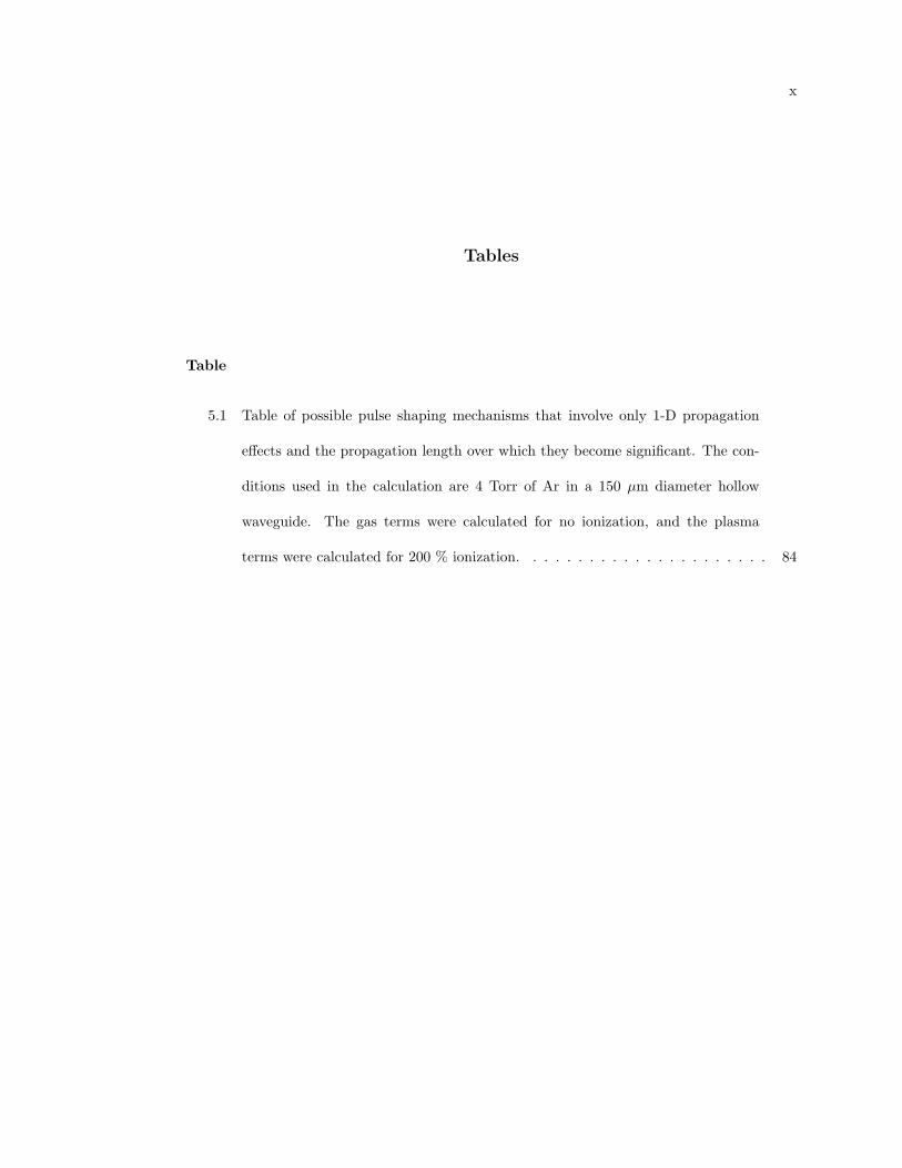
5.1 Table of possible pulse shaping mechanisms that involve only 1-D propagation

effects and the propagation length over which they become significant. The con-

ditions used in the calculation are 4 Torr of Ar in a 150 µm diameter hollow

waveguide. The gas terms were calculated for no ionization, and the plasma

terms were calculated for 200 % ionization. . . . . . . . . . . . . . . . . . . . . . 84

xi

Figures

Figure

2.1 Plot of pressure for phase matching as a function of normalized ionization fraction

(η/ηcr). Beyond critical ionization, phase matching is no longer possible. . . . . . 9

2.2 Diagram of quasi-phase matching plotting the second harmonic signal for the

conditions of: A. Perfect phase matching, C. No phase matching, B1. First-order

QPM, and B3. Third-order QPM. From [27]. . . . . . . . . . . . . . . . . . . . . 10

2.3 a. Calculation of the signal of the 95th harmonic for a straight waveguide as a

function of propagation distance. b. Calculation for a 0.5 mm period modulated

waveguide. From [19]. . . . . . . . . . . . . . . . . . . . . . . . . . . . . . . . . . 12

2.4 Optical microscope image of a 0.25 mm period modulated waveguide manufac-

tured by glass-blowing techniques. From [31]. . . . . . . . . . . . . . . . . . . . . 14

2.5 Experimental harmonic spectra from modulated waveguides filled with 111 Torr

He with a driving pulse of 25 fs and peak intensity ∼ 5 x 1014 W/cm2, for different

modulation periodicities. From [56]. . . . . . . . . . . . . . . . . . . . . . . . . . 15

2.6 Harmonic spectra from straight (black), 0.5 mm (blue), and 0.25 mm (red) pe-

riodicity modulated waveguides filled with 6 Torr neon. The spectra were taken

using the SC grating and a 10 second exposure time. . . . . . . . . . . . . . . . . 17

xii

2.7 Harmonic emission from straight (black) and 0.25 mm (red) modulated waveg-

uides filled with 7 Torr Ar. From [31]. The spectra were taken using the SC

grating. The exposure time for the straight waveguide was 300 seconds while for

the modulated it was 200 seconds. The spectrum for the modulated waveguide

has been multiplied by 1.5 for comparison. . . . . . . . . . . . . . . . . . . . . . . 18

2.8 Harmonic spectra from a straight waveguide filled with 10 Torr Ar (blue) and 6

Torr Ar (black), and a 0.25 mm modulated waveguide with 5 Torr Ar(red). All

spectra were taken with the SC grating. Both straight waveguide spectra have

a 300 s exposure time while the modulated waveguide spectrum was taken with

600 s exposure and divided by 2 for comparison. . . . . . . . . . . . . . . . . . . 19

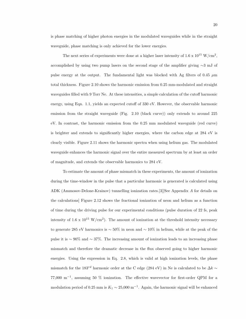
2.9 Harmonic spectra from straight, 0.5 mm, and 0.25 mm modulated waveguides,

with different pressures of neon gas. All spectra were taken with a 10 s exposure

time on the SC grating. Also plotted are the integrated counts for three different

photon energy ranges as a function of pressure. The energy ranges are indicated

with dashed lines. . . . . . . . . . . . . . . . . . . . . . . . . . . . . . . . . . . . . 21

2.10 Experimental harmonic spectra generated in 9 Torr of neon gas for straight (black)

and 0.25 mm modulated (red) waveguides. Both spectra taken with a 180 s

exposure time on the SB grating. From [31]. . . . . . . . . . . . . . . . . . . . . . 22

2.11 Experimental harmonic spectra generated in helium at 15 Torr using a 0.25 mm

modulated waveguide (black), and at 16 Torr (blue) and 10 Torr (red) using a

straight waveguide. All spectra taken with 120 s exposure on SB grating. . . . . 23

2.12 Calculation of the fractional ionization of neon and helium as a function of time

during the laser pulse. The right axis plots the cutoff photon energy corresponding

to the instantaneous pulse intensity. . . . . . . . . . . . . . . . . . . . . . . . . . 24

2.13 Comparison of harmonic spectra at the C edge using a 0.25 mm modulated waveg-

uide filled with 9 Torr Ne (black), 42 Torr He (blue), and 60 Torr He (red). All

spectra taken with 180 s exposure time using SB grating. . . . . . . . . . . . . . 26

xiii

2.14 Comparison of harmonic spectra from 8 Torr Ne (black) and 15 Torr He (red)

using a 0.25 mm modulated waveguide. Both spectra taken with 120 s exposure

time using SB grating. . . . . . . . . . . . . . . . . . . . . . . . . . . . . . . . . . 27

2.15 Calculations of the radial profile of the intensity (red curve) and phase (green

curve) of the laser inside the modulated waveguide. The three frames correspond

to: a. the initial mode, b. the mode giving the maximum on-axis intensity and

c. the minimum on-axis intensity. From Ivan Christov. . . . . . . . . . . . . . . . 29

2.16 Diagram showing region in pulse where a given harmonic, only generated above

the threshold intensity, is turned on and off by a 10% intensity modulation. . . . 31

2.17 Plot of absorption length as a function of photon energy for 10 Torr Neon and

100 Torr Helium. Data from the Center for X-ray Optics, Berkeley Lab (www-

cxro.lbl.gov). . . . . . . . . . . . . . . . . . . . . . . . . . . . . . . . . . . . . . . 32

2.18 Comparison of ionization fraction of neon as a function of time for a 22 fs duration

pulse at different peak intensities. . . . . . . . . . . . . . . . . . . . . . . . . . . . 35

2.19 Harmonic intensity as a function of propagation distance for the case where the

phase mismatch varies sinusoidally by 1, 3, and 5 % with a period of 2 coherence

lengths. . . . . . . . . . . . . . . . . . . . . . . . . . . . . . . . . . . . . . . . . . 36

2.20 Plot of the harmonic intensity during the first 60 coherence lengths. . . . . . . . 37

2.21 Return phase, φf , as a function of the release phase, φ0, determined by the

classical equations of motion. . . . . . . . . . . . . . . . . . . . . . . . . . . . . . 40

2.22 Electron return kinetic energy for trajectories with different release phases, φ0.

The long and short trajectories are indicated. . . . . . . . . . . . . . . . . . . . . 40

2.23 Intrinsic phase as a function of harmonic energy. The long trajectories acquire

more phase than the short trajectories. . . . . . . . . . . . . . . . . . . . . . . . . 41

2.24 Plot of harmonic phase in reference to the fundamental as a function of harmonic

energy. Note there is a linear dependence which is different for the long and short

trajectories. . . . . . . . . . . . . . . . . . . . . . . . . . . . . . . . . . . . . . . . 41

xiv

2.25 Plot of the intensity dependence of the harmonic phase for two different harmonic

orders. The calculation was done for a fundamental wavelength of 800 nm. . . . 42

2.26 Calculation of the phase mismatch (∆k) for the 171st harmonic in 3 Torr neon

for a 20 fs duration pulse with a peak intensity of 1015 W/cm2. The dashed line

indicates when the QPM condition is met for a modulation period of 0.25 mm. . 44

2.27 Calculation of the harmonic signal of the 171st harmonic in 3 Torr neon for a 20

fs duration pulse with a peak intensity of 1015 W/cm2 by quasi-phase matching

with 0.25 mm periodicity. Here, the propagation length is 1 mm. . . . . . . . . . 44

2.28 Calculation of the harmonic spectra for (a) a straight waveguide and (b) a 0.5

mm periodicity modulated waveguide for a 15 fs duration pulse with an intensity

of 7 x 1014 W/cm2 in 1 Torr Ar. The calculated single atom spectrum is also

shown. . . . . . . . . . . . . . . . . . . . . . . . . . . . . . . . . . . . . . . . . . . 46

2.29 Calculation of the time dependence of the harmonic output for (a) the straight

waveguide and (b) the 0.5 mm periodicity modulated waveguide. . . . . . . . . . 47

2.30 a. Calculation of the flux of the 29th harmonic for a 20 fs laser pulse and peak

intensity of 2.2 x 1014 W/cm2 as a function of argon pressure using a 3 cm

waveguide. b. Experimentally measured flux for the same conditions as part a.

From [26]. . . . . . . . . . . . . . . . . . . . . . . . . . . . . . . . . . . . . . . . . 48

2.31 Calculation of the fractional ionization of argon using ADK ionization rates for a

20 fs pulse with peak intensity of 2.2 x 1014 W/cm2 for a cosine (black) and sine

(red) pulse. . . . . . . . . . . . . . . . . . . . . . . . . . . . . . . . . . . . . . . . 49

3.1 Harmonic emission from argon using a gas jet with 250 mJ pulse energy and a

250 fs pulse. From [80] . . . . . . . . . . . . . . . . . . . . . . . . . . . . . . . . . 52

xv

3.2 Harmonic emission from a straight 150 µm inner diameter, 2.5 cm long fiber filled

with low-pressure Ar (7 Torr), driven by an 800 nm laser with an 18 fs pulse

duration and a peak intensity of 9 x 1014 Wcm−2. The spectrum was taken using

the SC grating and an exposure time of 300 s. . . . . . . . . . . . . . . . . . . . . 54

3.3 Harmonic emission at a higher peak laser intensity of 1.3 x 1015 Wcm−2, using

a 0.25 mm period modulated waveguide. The spectrum was taken using the SC

grating with a 600 s exposure time. . . . . . . . . . . . . . . . . . . . . . . . . . . 55

3.4 Calculated ionization levels in argon for an 18 fs laser pulse at a peak laser

intensity of 1.3 x 1015 Wcm−2, using ADK rates. Laser pulse (black dashed); Ar

(red); Ar+ (green); Ar++ (blue). The right axis shows the predicted HHG cutoff

energy for the laser intensity profile, calculated from the cutoff rule. . . . . . . . 57

3.5 Calculated ionization rates of argon species for the same conditions as in Fig. 3.4. 57

3.6 Calculated harmonic emission from neutral (red) and singly ionized Ar (blue) for

an 18 fs laser pulse centered at 800 nm, at a laser intensity of 1.3 x 1015 Wcm−2.

The ion spectrum has not been corrected for the dynamically varying populations. 58

3.7 Static ionization rates of H and He versus electric field strength. Solid line:

numerical calculations of TDSE. Dashed line: ADK theory. From [66]. . . . . . . 60

3.8 Fraction of ionized H in the BSI regime as a function of the peak electric field

amplitude for pulses of 5, 10, and 20 fs in duration. Full line is ADK model, trian-

gles show Krainov model, and circles show time-dependent Schroedinger equation.

The dotted line is Ebs for H. From [71]. . . . . . . . . . . . . . . . . . . . . . . . 61

3.9 Measured harmonic spectra from a straight waveguide filled with argon at 5 Torr

(red) and 7 Torr (black) for a pulse peak intensity of ∼ 9 x 1014 Wcm−2. Both

spectra taken with the SC grating and an exposure time of 300 s (using 0.4 µm

thick Zr filters). . . . . . . . . . . . . . . . . . . . . . . . . . . . . . . . . . . . . . 64

xvi

3.10 Harmonic spectra from a straight waveguide filled with Ne at different pressures

for a peak laser intensity of ∼ 9 x 1014 Wcm−2. All spectra taken with the SC

grating and a 10 s exposure (using 0.4 µm thick Zr filters). . . . . . . . . . . . . 64

4.1 Schematic of Ti:Sapphire amplifier system used for high harmonic generation. . . 67

4.2 Schematic of experimental setup for the generation and measurement of high

harmonics. . . . . . . . . . . . . . . . . . . . . . . . . . . . . . . . . . . . . . . . . 68

4.3 Harmonic spectra generated in neon using 0.2 µm-thick B (black) and 0.18 µm-

thick Si (red) filters to calibrate the SC grating. . . . . . . . . . . . . . . . . . . . 70

4.4 Harmonic spectra generated in neon using 0.2 µm-thick B (black) and C (red)

filters to calibrate the SB grating. . . . . . . . . . . . . . . . . . . . . . . . . . . . 71

4.5 Schematic of grazing incidence grating and relevant angles. . . . . . . . . . . . . 71

4.6 Wavelength and energy calibration of SC grating using the grating equation and

a two point linear fit. . . . . . . . . . . . . . . . . . . . . . . . . . . . . . . . . . . 71

4.7 Wavelength and energy calibration of SB grating using the grating equation and

a two point linear fit. . . . . . . . . . . . . . . . . . . . . . . . . . . . . . . . . . . 72

4.8 Reflectivity of a Au mirror at 2 degree grazing incidence angle for the ideal case,

and for 2 nm RMS surface roughness. . . . . . . . . . . . . . . . . . . . . . . . . 74

4.9 Measured efficiency of SB grating as a function of photon energy. . . . . . . . . . 74

4.10 Harmonic spectra at the carbon edge showing the data points used to estimate

the photon flux. . . . . . . . . . . . . . . . . . . . . . . . . . . . . . . . . . . . . . 76

4.11 Measured flux from the ALS beamline 6.1 and estimated flux assuming 100%

efficient optics (dashed line). From [76]. . . . . . . . . . . . . . . . . . . . . . . . 76

5.1 Spectra taken after the 2.5 cm long, 150 µm diameter waveguide with different

Ar pressures. . . . . . . . . . . . . . . . . . . . . . . . . . . . . . . . . . . . . . . 79

xvii

5.2 Deconvolved FROG measurements of the temporal pulse shape before and after

the waveguide with different Ar pressures for an initial pulse of 32 fs. The pulse

FWHM for the different measurements are indicated. . . . . . . . . . . . . . . . . 80

5.3 Deconvolved FROG measurements of the temporal pulse shape before and after

the waveguide with different Ar pressures for an initial pulse of 29 fs. At 4 Torr,

the final pulse duration is 13.3 fs FWHM. From [78]. . . . . . . . . . . . . . . . . 81

5.4 Comparison of the measured spectrum with the spectrum from FROG measure-

ment deconvolution. . . . . . . . . . . . . . . . . . . . . . . . . . . . . . . . . . . 81

5.5 Theoretical calculation of temporal pulse shape after the waveguide with different

Ar pressures for an initial pulse duration of 30 fs using the 3-D propagation model.

The pulse FWHM are indicated. . . . . . . . . . . . . . . . . . . . . . . . . . . . 86

5.6 Theoretical calculation of the pulse spectrum before and after the waveguide with

different Ar pressures. . . . . . . . . . . . . . . . . . . . . . . . . . . . . . . . . . 87

6.1 Diagram of magnetic bottle showing direction of field lines and electron trajectories. 90

6.2 Schematic of compact magnetic bottle time-of-flight spectrometer. Dimensions

are indicated. . . . . . . . . . . . . . . . . . . . . . . . . . . . . . . . . . . . . . . 92

6.3 Measured values of the magnetic field on axis above a 1 inch dia., 0.5 inch thick,

NdFeB magnet (black dots). Theoretical prediction of magnetic field for a magnet

with a magnetization of 8000 A/m (red line). . . . . . . . . . . . . . . . . . . . . 94

6.4 Calculated z component of the magnetic field from the permanent magnet and

solenoid on axis. . . . . . . . . . . . . . . . . . . . . . . . . . . . . . . . . . . . . 95

6.5 Calculated adiabatic parameter on axis, for 1 eV electrons. . . . . . . . . . . . . 96

6.6 Calculated (dashed) and measured (solid) magnetic field and adiabatic parameter

for 1 eV electrons on axis. From [43]. . . . . . . . . . . . . . . . . . . . . . . . . . 96

6.7 High harmonic spectrum measured by the magnetic-bottle photoelectron spec-

trometer using different detection gases. . . . . . . . . . . . . . . . . . . . . . . . 97

xviii

6.8 Absorption at different photon energies for argon and neon gas. From CXRO

website. . . . . . . . . . . . . . . . . . . . . . . . . . . . . . . . . . . . . . . . . . 98

6.9 Photoelectron spectrum of HHG from Ne extending to ∼ 100 eV photon energies. 99

6.10 Comparison of photon spectra measured using the magnetic bottle photoelectron

spectrometer and the Hettrick spectrometer. . . . . . . . . . . . . . . . . . . . . . 100

6.11 Diagram of resonant and non-resonant Auger processes in xenon. . . . . . . . . . 100

6.12 Photoelectron spectrum of xenon using all harmonics (blue) and harmonics pass-

ing through an Al filter blocking energies > 65 eV (red). . . . . . . . . . . . . . . 102

6.13 Absorption of xenon gas as a function of photon energy. Data from the Center

for X-ray Optics, Berkeley Lab (www-cxro.lbl.gov). . . . . . . . . . . . . . . . . . 102

6.14 Reflectivity as a function of photon energy for the Si/Mo multilayer mirror, mea-

sured at an 85 degree incident angle. . . . . . . . . . . . . . . . . . . . . . . . . . 103

6.15 Spectra of high harmonics generated using He gas and detected with Ne gas before

(black) and after (red) the narrow-band multilayer mirror. . . . . . . . . . . . . . 104

6.16 Photoelectron spectrum of Xe using a narrow bandwidth of harmonics selected

by the multilayer mirror. . . . . . . . . . . . . . . . . . . . . . . . . . . . . . . . . 104

6.17 Schematic of experimental setup for measuring the pulse duration of high har-

monic generation. . . . . . . . . . . . . . . . . . . . . . . . . . . . . . . . . . . . . 105

6.18 Photoelectron spectra at different probe delays. The sidebands that are analyzed

are indicated. . . . . . . . . . . . . . . . . . . . . . . . . . . . . . . . . . . . . . . 106

6.19 Integrated counts for the sidebands at 22 and 25 eV as a function of probe delay. 106

C.1 MCP detector design. The micro-channel plates are in dark blue. The anode is

biased at 2 kV and is insulated from the grounded stainless steel housing. . . . . 121

C.2 Detailed schematic of the MCP detector giving dimensions for each part. All

dimensions are in inches. . . . . . . . . . . . . . . . . . . . . . . . . . . . . . . . . 122

Chapter 1

Introduction

Ultrafast laser technology makes it possible to generate extremely high field intensities

above 1018 W/cm2, or alternatively, to generate pulses with extremely short time durations cor-

responding to only a few femtoseconds (10−15 s).[8, 14] One of the most prominent applications

of very high-power, ultrashort-pulse lasers has been the study of non-perturbative light-matter

interactions. At intensities above 1014 W/cm2, the magnitude of the electric field of the laser

radiation is comparable to the field binding an electron to an atom. In this regime, the laser

field can easily ionize atoms. Once the atom is ionized, the subsequent motion of the free elec-

tron is controlled by the oscillating laser field, and the electron can easily reach kinetic energies

many times that of the original electron binding energy. One significant consequence of this in-

tense light-matter interaction is the process of high-order harmonic generation (HHG).[51, 28]

In HHG, the free electron recollides with its parent ion and recombines with it, releasing a high

energy photon. Since all atoms experience the same coherent laser field, the harmonic radiation

is also highly coherent. Temporally, high harmonic radiation is a series of attosecond-duration

bursts occurring every half-cycle of the driving laser. This unique property has allowed measure-

ments of electronic processes in atoms occurring on timescales previously inaccessible.[40, 24]

The emission from HHG can extend from the ultraviolet up to the soft x-ray region of the

spectrum (to ∼ 950 eV). This spectral region is interesting for studies of chemical and material

processes because these photon energies can access valence and inner shell electrons of atoms

and molecules.[11, 33, 55] Also, HHG is an extremely useful light source for applications such as

2

plasma interferometry[23, 60] or extreme-ultraviolet (EUV) lithography, a technology that will

be needed to implement the next generation of integrated circuits. Thus, high harmonic gener-

ation has both fundamental and practical applications. However, one major problem is that the

efficiency of HHG is extremely low, typically on order of 10−5 to 10−10 conversion of laser energy

into each harmonic order. As with any harmonic generation process, the efficiency can be greatly

enhanced by phase matching. Traditional optical phase matching techniques have been applied

successfully to high harmonic generation for low harmonic orders (< 90 eV).[62, 26] However,

before now there were no techniques for enhancement of HHG at higher photon energies.

In this thesis, I will present two major breakthroughs in the field of high harmonic

generation. First, I will discuss work on quasi-phase matching of high harmonic generation,

which has allowed increased conversion efficiency of high harmonic light up to the water window

region of the soft X-ray spectrum (∼ 300 eV) for the first time.[31] This spectral region is

significant because at these photon energies, water is transparent while carbon strongly absorbs,

making it a useful light source for very high resolution contrast microscopy on biological samples.

Since the resolution is on order of the wavelength of the light (∼ 4 nm for 300 eV), detailed

structures of cells and DNA can be viewed. A table-top source of light in the water window soft

X-ray region would greatly benefit biological and medical research. Second, I will present work

on the generation of very high harmonic orders from ions. This work is the first to show that

harmonic emission from ions is of comparable efficiency to emission from neutral atoms thereby

showing that high harmonic emission is not limited by the saturation intensity, or the intensity

at which the medium is fully ionized, but can extend to much higher photon energies.[30] Both

results were obtained by using a waveguide geometry for HHG, allowing manipulation of the

phase matching conditions and reducing the detrimental effects of ionization. The ideas from this

work are expected to increase the number of applications of high harmonic generation as a light

source by increasing the efficiency of the process and opening up the possibility of generating

multi-keV photon energies.

3

1.1 High-order Harmonic Generation

High-order harmonic generation occurs when an intense linearly polarized laser field in-

teracts with a gas or material. An intuitive model of HHG at the atomic level was developed

by Corkum, Kulander, and others,[22, 44] and is sometimes referred to as the three-step model.

In the first step, the strong electric field of the laser suppresses the Coulomb barrier binding

an electron to an atom, freeing the valence electron either by tunnelling or by over-the-barrier

ionization. The freed electron is then accelerated by the field. Since the laser field is oscillat-

ing, the electron can with some probability return to its parent ion and recombine, emitting a

high-energy photon. This process occurs for many atoms driven coherently over several laser

cycles, resulting in emission of higher-order odd harmonics of the fundamental in a coherent,

low-divergence beam. The three-step model accurately predicts that the highest photon energy

that can result from HHG occurs when an electron is ionized at a phase corresponding to 18

degrees after the peak of the laser cycle. This cutoff photon energy is predicted to be:

Emax = Ip + 3.2Up, (1.1)

where Ip is the ionization potential of the atom and Up is the ponderomotive energy given by:

Up = e2E2/4mω2 = 9.33× 10−14Iλ2eV, (1.2)

where e, E, m, ω, I, and λ are the electron charge, field amplitude, electron mass, fundamental

laser frequency, intensity in W/cm2, and wavelength in microns respectively. The highest photon

energy therefore scales linearly with the laser intensity.

The recollision energies associated with the intensities required to field-ionize atoms can

be as high as hundreds of electron volts.[15, 70, 67] Thus, the emitted high-harmonic pho-

tons can correspond to the combined energy of several hundred incident photons. The linear

relationship between the cutoff and the incident intensity presents a very attractive scaling as

compared to, for example, EUV laser schemes where the power requirements scale as the photon

energy to the 3rd-5th power.[39] However, to take advantage of this favorable scaling, several

4

challenges must be overcome. The HHG process necessarily ionizes the medium, generating a

free-electron plasma. The dispersion of the plasma creates a mismatch in the phase velocities

of the fundamental and harmonic light, significantly reducing the amount of harmonic signal

produced. Also, the generated plasma can defocus the laser beam, decreasing the peak intensity

and thereby limiting the maximum harmonic energy.[48] To date, the highest energy HHG emis-

sion has been achieved using short-duration laser pulses and noble gases with high ionization

potentials such as helium, which can reduce the amount of ionization for a given peak inten-

sity. However, helium has a small cross-section giving it a lower efficiency for HHG than larger,

multi-electron atoms. In Ch. 3, I will discuss a method of generating high harmonics even in a

fully ionized gas medium, allowing HHG in argon up to photon energies of 250 eV, previously

achieved only with He gas, and demonstrating that HHG from ions is feasible. In combination

with quasi-phase matching techniques, this method should extend the efficient energy range of

HHG even further.

The simple semi-classical picture of HHG as given by the three-step model accurately

predicts the range of photon energies that can be obtained for a given incident laser intensity.

However, a quantum mechanical treatment is needed for a more complete picture of the HHG

process. In the quantum picture, as the laser field strength increases, portions of the electron

wave function tunnel through the suppressed atomic barrier and then propagate large distances -

relative to the atomic radius - away from the atom. When the laser field reverses, this extended

electron wavefunction re-encounters the part of the wavefunction still in the ground state of

the atom, leading to quantum interferences. As a result, rapid oscillations in the electronic

probability distribution and therefore the transient dipole moment of the atom lead to the

emission of very high-order harmonics of the fundamental laser.

A fully quantum, analytical theory of HHG, derived by Lewenstein et al.[46], has been

extremely successful in describing both the general characteristics of HHG such as the photon

energy cutoff, as well as more specific characteristics such as the divergence properties of the

generated beam[9] and the specific spectral characteristics of the emission. Qualitatively, the

5

spectral characteristics of HHG emission are a result of the fact that the freed electron has an

associated deBroglie wavelength corresponding to the kinetic energy acquired in the laser field,

λ = h/p, where h is Planck’s constant and p is the electron momentum. The emission also has a

phase related to the total phase the electron accumulates during its free trajectory, given by:[9]

Φ = qωtf − S(pst, ti, tf )/h̄, (1.3)

where q is the harmonic order, ω is the laser frequency, ti is the time the electron is released

in the laser field, tf is the recollision time, and S(pst, ti, tf ) is the semi-classical action over

the electron’s trajectory. The phase of the emitted harmonic light is therefore not simply re-

lated to the phase of the driving laser, but also includes an intrinsic phase component that

can vary rapidly with laser intensity. The intrinsic phase has consequences for both the spa-

tial and spectral emission characteristics. Spatially, the intrinsic phase can result in a complex

spatial profile of the harmonic emission when generated using a beam that is converging to-

ward a focus. This is in contrast to the gaussian spatial profile for HHG generated by a beam

diverging from a focus[9, 63, 58] or the full spatial coherence of light generated using a waveg-

uide configuration.[49] In the spectral domain, this time-varying intrinsic phase results in large

frequency shifts and spectral broadening or narrowing of the harmonic emission.[16] The intrin-

sic phase also plays a role in quasi-phase matching of HHG as will be discussed in the next

chapter.

Chapter 2

Quasi-Phase Matching

Applications of HHG radiation as a table-top, coherent soft X-ray source depend upon

optimizing the total flux generated. In nonlinear optical processes, the conversion efficiency

from the fundamental to the harmonic field is enhanced by phase matching. In its simplest

manifestation, phase matching will occur when the driving laser and the harmonic signal travel

with the same phase velocity, so that signal generated throughout the conversion region adds

constructively. In HHG, since the ionization level is changing throughout the pulse, and the

increasing density of free electrons has a large effect on the phase velocity of the driving laser,

phase matching can only be obtained in limited time windows in the pulse. Experimentally,

dramatic enhancement of the flux from HHG can be achieved by pressure-tuned phase matching

using hollow-core gas-filled waveguides.[62, 26] The laser light is guided by glancing-incidence

reflection off the waveguide walls, allowing propagation over an extended interaction length

with a well defined intensity and phase profile. The fundamental and harmonic light propagate

through the waveguide with phase velocities determined by the dispersion of the neutral gas,

the plasma, and the waveguide at the two different frequencies. The phase mismatch is given

by ∆k = qkf − kq, where kf is the wavevector of the fundamental and kq is the wavevector of

harmonic order q. The full expression is given by:

∆k = ∆kWaveguide + ∆kPlasma + ∆kNeutrals (2.1)

7

or

∆k =qu2

11λ

4πa2+ PηNatmre(qλ− λ/q)− 2π(1− η)Pq∆δ

λ, (2.2)

where λ, q, a, u11, η, P, Natm, and re are the fundamental wavelength, harmonic order, waveguide

radius, the first zero of the Bessel function J0, ionization fraction, gas pressure in atmospheres,

number density at 1 atm, and classical electron radius respectively, and ∆δ is the difference in

the index of refraction at the fundamental and harmonic frequencies of the generation gas at

1 atm. Here, the small contribution from the nonlinear refractive index is neglected and it is

assumed that the harmonic light does not interact with the waveguide. The waveguide allows

control over the experimental parameters such as gas pressure and radius to optimize phase

matching.

For low levels of ionization, the pressure can be adjusted so that the waveguide and plasma

dispersion balance the dispersion due to the neutral atoms, which is of opposite sign, and phase

matching can be achieved (∆k = 0). Since phase matching is accomplished by adjusting the

phase velocity of the fundamental, and the harmonic radiation travels at a phase velocity of

∼c, the bandwidth of phase matching is very broad, encompassing many harmonic orders. At

higher laser intensities, the rapidly-changing ionization during the pulse means that there is a

limited time-window for phase matching. However, the phase matching bandwidth is also broad

since the phase matching condition for different harmonic orders will occur at some time during

the pulse. When phase matched, the harmonic signal increases quadratically with interaction

length until it is limited by absorption of the harmonic light by the gas medium.

Unfortunately, this method of phase matching is limited to low ionization levels. When

a large enough fraction of the gas is ionized, the plasma dispersion is greater than the neutral

dispersion for any pressure so that phase matching is no longer possible. The phase velocity

of the fundamental light then exceeds that of the generated harmonic signal. The value of this

critical ionization fraction is given by:[61]

ηcr = (1 +Natmreλ

2

2π∆δ)−1. (2.3)

8

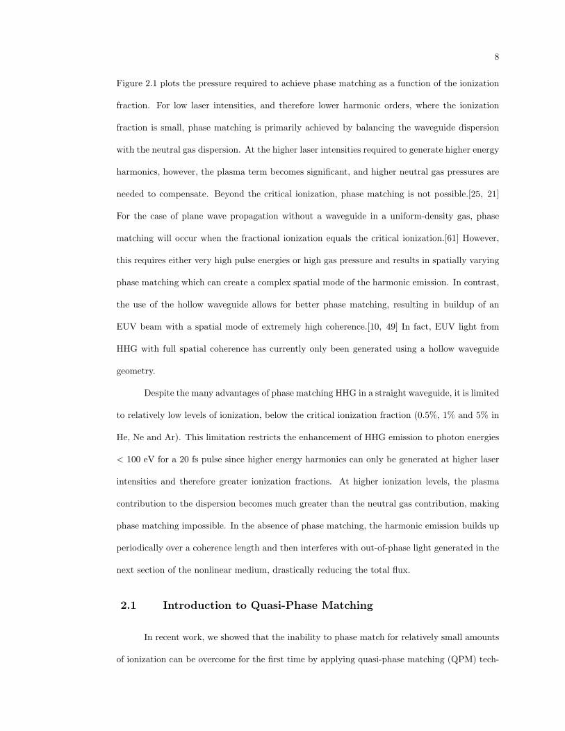
Figure 2.1 plots the pressure required to achieve phase matching as a function of the ionization

fraction. For low laser intensities, and therefore lower harmonic orders, where the ionization

fraction is small, phase matching is primarily achieved by balancing the waveguide dispersion

with the neutral gas dispersion. At the higher laser intensities required to generate higher energy

harmonics, however, the plasma term becomes significant, and higher neutral gas pressures are

needed to compensate. Beyond the critical ionization, phase matching is not possible.[25, 21]

For the case of plane wave propagation without a waveguide in a uniform-density gas, phase

matching will occur when the fractional ionization equals the critical ionization.[61] However,

this requires either very high pulse energies or high gas pressure and results in spatially varying

phase matching which can create a complex spatial mode of the harmonic emission. In contrast,

the use of the hollow waveguide allows for better phase matching, resulting in buildup of an

EUV beam with a spatial mode of extremely high coherence.[10, 49] In fact, EUV light from

HHG with full spatial coherence has currently only been generated using a hollow waveguide

geometry.

Despite the many advantages of phase matching HHG in a straight waveguide, it is limited

to relatively low levels of ionization, below the critical ionization fraction (0.5%, 1% and 5% in

He, Ne and Ar). This limitation restricts the enhancement of HHG emission to photon energies

< 100 eV for a 20 fs pulse since higher energy harmonics can only be generated at higher laser

intensities and therefore greater ionization fractions. At higher ionization levels, the plasma

contribution to the dispersion becomes much greater than the neutral gas contribution, making

phase matching impossible. In the absence of phase matching, the harmonic emission builds up

periodically over a coherence length and then interferes with out-of-phase light generated in the

next section of the nonlinear medium, drastically reducing the total flux.

2.1 Introduction to Quasi-Phase Matching

In recent work, we showed that the inability to phase match for relatively small amounts

of ionization can be overcome for the first time by applying quasi-phase matching (QPM) tech-

9

∆ k = 0

NoPhaseMatching

Figure 2.1: Plot of pressure for phase matching as a function of normalized ionization fraction(η/ηcr). Beyond critical ionization, phase matching is no longer possible.

10

niques to the HHG process. The ability to quasi-phase match HHG significantly extends the

range of photon energies where it is possible to generate high-harmonic emission efficiently.

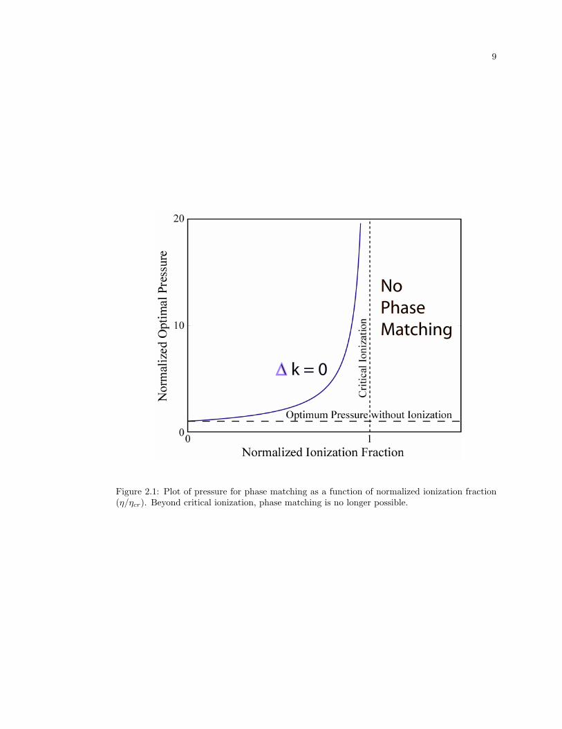
Quasi-phase matching was first proposed in 1962, shortly after the birth of nonlinear optics.

Armstrong et al.[4] proposed a phase corrective scheme whereby the phase mismatch in a non-

linear optical process is periodically corrected by introducing a periodicity to the nonlinearity

of the medium corresponding to the coherence length. The coherence length is defined as the

distance it takes for the fundamental and harmonic light to become 180 degrees out of phase.

For example, quasi-phase matching of second harmonic light can be achieved by periodically

reversing the crystal orientation and therefore the polarity of the nonlinear response so that

a 180 degree phase shift is introduced every coherence length. This reverses the destructive

interference, allowing continual buildup of the harmonic signal, shown in Fig. 2.2. Practical im-

plementation of this concept was not achieved until the development of crystal-poling techniques

in the mid-1990’s.[27]

Figure 2.2: Diagram of quasi-phase matching plotting the second harmonic signal for the con-ditions of: A. Perfect phase matching, C. No phase matching, B1. First-order QPM, and B3.Third-order QPM. From [27].

Unfortunately, the generation of coherent light at EUV and soft X-ray wavelengths must

take place in a gas or on a surface, making the use of standard QPM techniques impossible.

However, the extreme nonlinear nature of HHG makes alternate approaches possible. For ex-

ample, quasi-phase matching of the frequency conversion process can be achieved by restricting

11

HHG to regions where the signal will be in phase and add constructively. Previous theoretical

ideas for quasi-phase matching of HHG include using a modulated density gas or plasma to

periodically change the nonlinear susceptibility.[69] Another proposal suggested using counter-

propagating light to modulate the intensity and phase of the driving laser.[77] Experimentally,

quasi-phase matching of HHG was first implemented using a technique proposed by Christov et

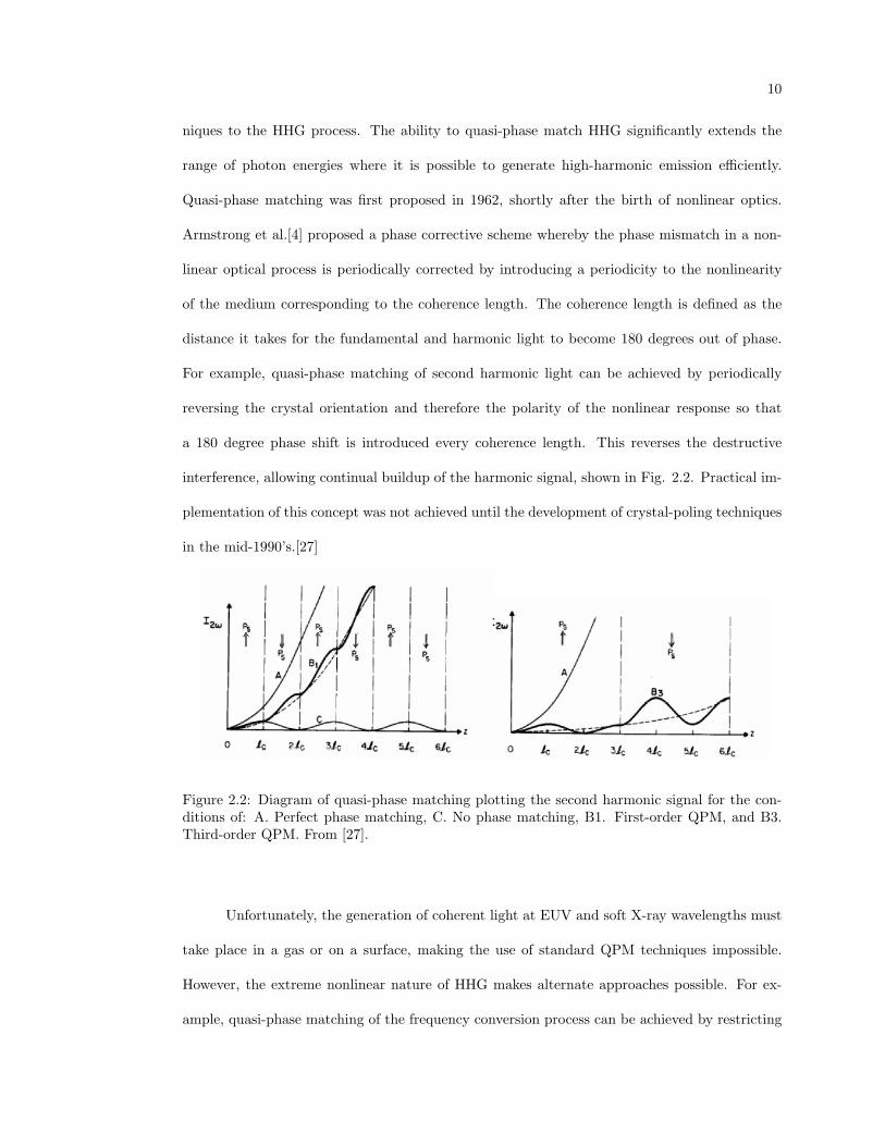
al.[19] In this technique, high harmonics are generated in a hollow-core waveguide which has a

periodically changing inner diameter along the length of the guide to modulate the driving laser

intensity. The modulation of the laser intensity effectively turns on and off the generation of

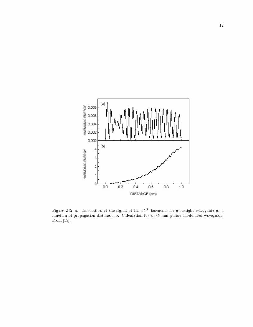
harmonics near the cutoff. Figure 2.3.a shows a calculation of the signal of the 95th harmonic, in

the cutoff, as a function of propagation length in a straight waveguide using a 15 fs pulse with a

peak intensity of 7 x 1014 W/cm2 and 1 Torr of argon. The calculation uses a three-dimensional

propagation model and the harmonic signal is calculated using a quasi-classical approximation

for the dipole moment. The oscillations of the harmonic signal are a result of the phase mismatch

as signal builds up over a coherence length and then interferes with out-of-phase light in the

next coherence length. Figure 2.3.b shows the same calculation using a hollow-core waveguide

with a 0.5 mm period sinusoidal corrugation that changes the laser intensity on-axis by 5%.

The modulated waveguide causes a dramatic enhancement in the final signal (note the different

scales of the two plots).

We can understand the basic physics behind the enhancement of the HHG signal using

classical nonlinear optics theory. In a simplified model of harmonic generation, the field of

harmonic order q, after propagating a distance L in a nonlinear medium, is related to the phase

mismatch, ∆k, by:

Eq ∝∫ L

0

Enωd(z)e−i∆kzdz, (2.4)

where Eω is the fundamental field, n is the effective order of the nonlinear process, d(z) is the

nonlinear coefficient, and ∆k is the phase mismatch calculated in equation 4. To model quasi-

phase matching, the nonlinear coefficient is expressed as a general periodic function of z with

12

Figure 2.3: a. Calculation of the signal of the 95th harmonic for a straight waveguide as afunction of propagation distance. b. Calculation for a 0.5 mm period modulated waveguide.From [19].

13

period Λ:[27]

d(z) = deff

∞∑m=−∞

GmeiKmz, (2.5)

where Km = 2πm/Λ is the effective wavevector of QPM and m is the order of the QPM process.

Combining Eqns. 2.4 and 2.5 shows that the harmonic signal will be enhanced when Km ≈ ∆k.

The enhancement in signal will be greatest for m = 1, but the signal will also be enhanced

for higher order QPM (i.e. m = 3,5,...). The new quasi-phase matching condition for HHG is

therefore given by:

∆k = ∆kWaveguide + ∆kPlasma + ∆kNeutrals −Km (2.6)

or

∆k =qu2

11λ

4πa2+ PηNatmre(qλ− λ/q)− 2π(1− η)Pq∆δ

λ− 2πm/Λ. (2.7)

From Eqn. 2.7, it is evident that a larger value of Km, i.e. a shorter modulation period, can

compensate for a larger ∆k, and therefore a higher level of ionization.

2.2 Experimental Results on Quasi-Phase Matching of High Har-

monic Generation

The first set of experiments demonstrating quasi-phase matching of HHG showed a dra-

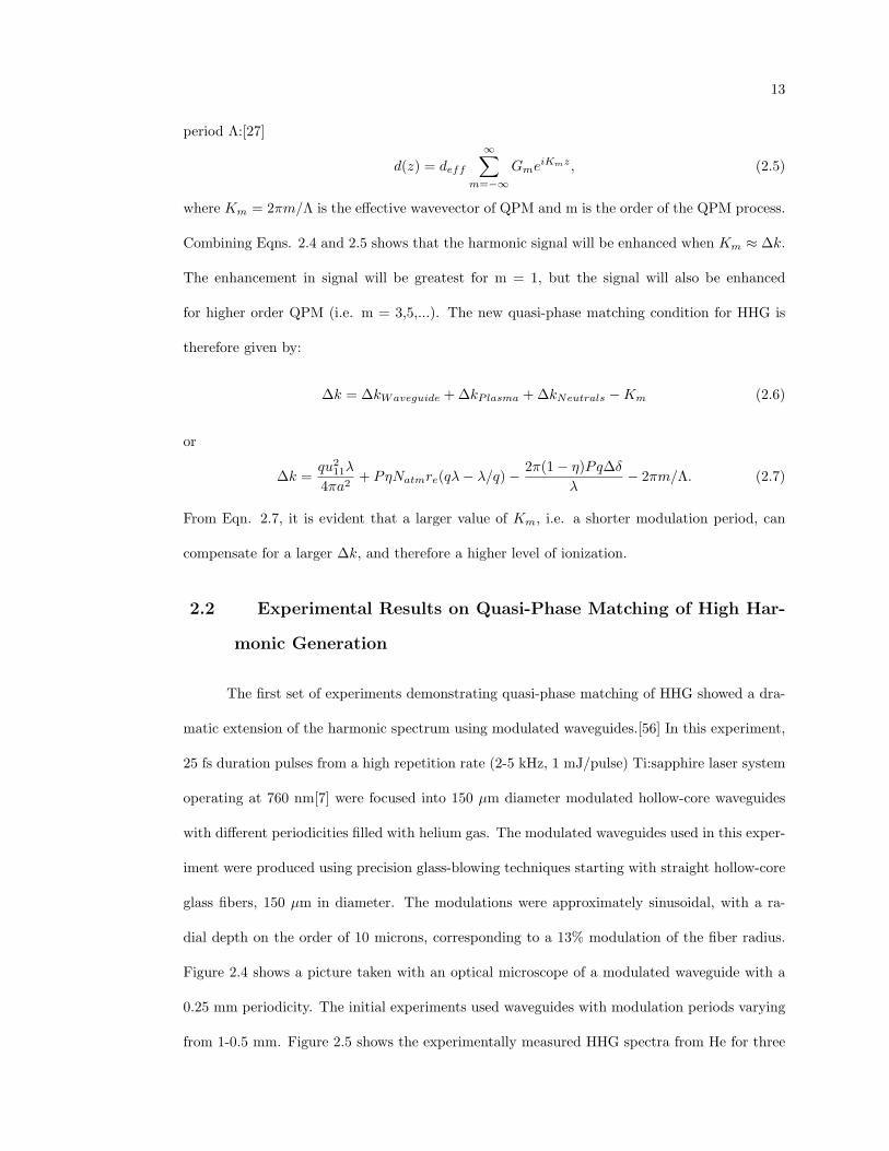
matic extension of the harmonic spectrum using modulated waveguides.[56] In this experiment,

25 fs duration pulses from a high repetition rate (2-5 kHz, 1 mJ/pulse) Ti:sapphire laser system

operating at 760 nm[7] were focused into 150 µm diameter modulated hollow-core waveguides

with different periodicities filled with helium gas. The modulated waveguides used in this exper-

iment were produced using precision glass-blowing techniques starting with straight hollow-core

glass fibers, 150 µm in diameter. The modulations were approximately sinusoidal, with a ra-

dial depth on the order of 10 microns, corresponding to a 13% modulation of the fiber radius.

Figure 2.4 shows a picture taken with an optical microscope of a modulated waveguide with a

0.25 mm periodicity. The initial experiments used waveguides with modulation periods varying

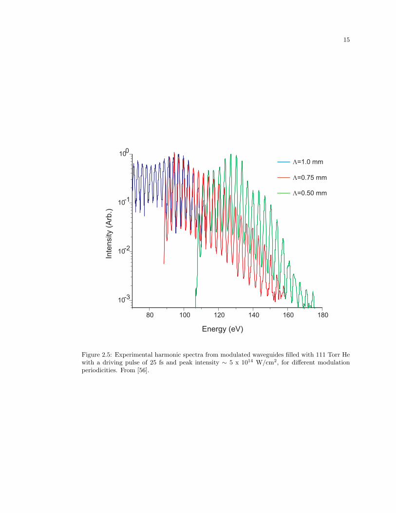
from 1-0.5 mm. Figure 2.5 shows the experimentally measured HHG spectra from He for three

14

different modulated-waveguide periodicities. As the modulation period is reduced from 1 mm

to 0.75 mm to 0.5 mm, the highest observable harmonic energy increases from 112 eV to 175 eV

and the signal is enhanced at higher and higher photon energies. This behavior agrees well with

the predictions from the simple QPM model that shorter modulation periods can compensate

for more ionization and thus phase match higher photon energies.

0.25 mm

150 Microns

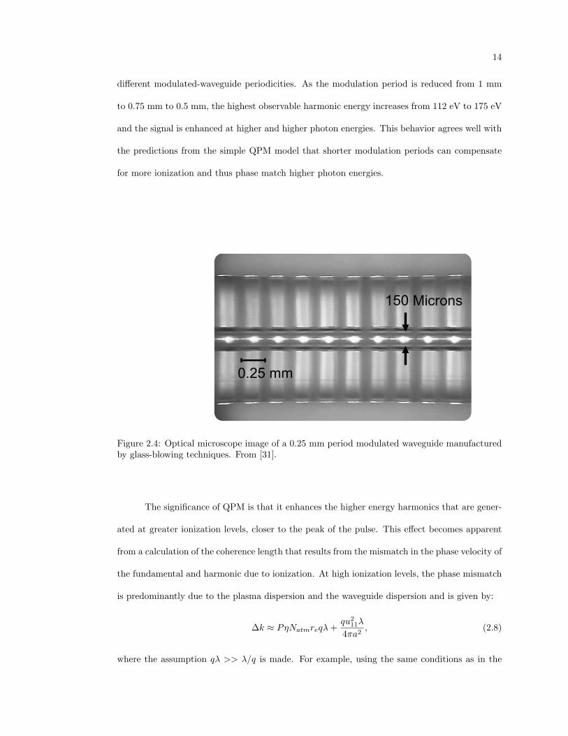
Figure 2.4: Optical microscope image of a 0.25 mm period modulated waveguide manufacturedby glass-blowing techniques. From [31].

The significance of QPM is that it enhances the higher energy harmonics that are gener-

ated at greater ionization levels, closer to the peak of the pulse. This effect becomes apparent

from a calculation of the coherence length that results from the mismatch in the phase velocity of

the fundamental and harmonic due to ionization. At high ionization levels, the phase mismatch

is predominantly due to the plasma dispersion and the waveguide dispersion and is given by:

∆k ≈ PηNatmreqλ +qu2

11λ

4πa2, (2.8)

where the assumption qλ >> λ/q is made. For example, using the same conditions as in the

15

Λ=1.0 mm

Λ=0.50 mm

Λ=0.75 mm

80 100 120 140 160 180

10-3

10-2

10-1

100

Inte

nsity

(Arb

.)

Energy (eV)

Figure 2.5: Experimental harmonic spectra from modulated waveguides filled with 111 Torr Hewith a driving pulse of 25 fs and peak intensity ∼ 5 x 1014 W/cm2, for different modulationperiodicities. From [56].

16

theory paper of Christov et al.,[19] fully ionized argon at a pressure of 1 Torr gives an electron

density of ne = 3.5 x 1016 cm−3. From equation 2.8, the phase mismatch of the 95th harmonic

order (150 eV) is calculated to be ∆kplasma ∼ 7550 m−1 and ∆kwaveguide ∼ 6200 m−1, giving

a total ∆k ∼ 13,750 m−1. The phase mismatch is close to the value of the effective QPM

wavevector for a modulation period of 0.5 mm of K1 ∼ 12,600 m−1. Thus, very substantial

levels of ionization can be compensated for by using waveguides with modulation periods in the

range of 1 - 0.25 mm that can be readily manufactured with glass-blowing techniques.

In the initial experiments, the ionization levels in He were still relatively low. However,

in more recent experiments, we have demonstrated QPM in much higher ionization levels of

> 100%. These experiments were performed using a two stage amplifier system (described in

Ch.4) with an output pulse energy of 1.2 mJ and a 22 fs pulse duration. Due to loss from mirror

reflections on the way to the waveguide setup, around 1.1 mJ pulse energy was focused into the

waveguide. The coupling efficiency was ∼ 60% for the straight, 0.5 mm, and 0.25 mm modulated

waveguides. The fundamental 800 nm light was blocked using a 0.4 µm-thick Zr filter with 25

nm of Ag coated on the front to prevent laser damage. Figure 2.6 shows harmonic spectra from

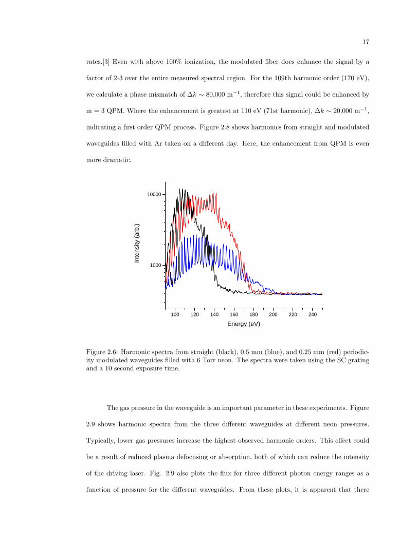
straight and modulated waveguides filled with neon gas. The same gas pressure of 6 Torr was

used in the different waveguides for comparison. The decrease in harmonic signal going to lower

photon energies is due to the decreasing transmission of the zirconium filter. As expected, the

modulated waveguides enhance the highest harmonic orders, and the signal from the 0.25 mm

modulated waveguide is about 8 times greater than from the 0.5 mm waveguide, showing the

ability of the shorter modulation periods to better compensate for the phase mismatch from

ionization. The higher harmonics observed from the 0.5 mm modulated fiber could be due to

a slightly better coupling efficiency. The estimated laser intensity in the waveguide is 9 x 1014

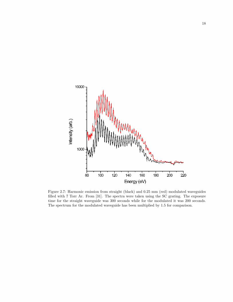
W/cm2, producing ∼ 24% ionization in neon at the peak of the pulse. Figure 2.7 shows the

harmonic spectra from straight and 0.25 mm modulated waveguides filled with 7 Torr Ar. Here,

the laser intensity is above the saturation intensity of argon so that the gas is fully ionized with

some double ionization, as verified using Ammosov-Delone-Krainov (ADK) tunnelling ionization

17

rates.[3] Even with above 100% ionization, the modulated fiber does enhance the signal by a

factor of 2-3 over the entire measured spectral region. For the 109th harmonic order (170 eV),

we calculate a phase mismatch of ∆k ∼ 80,000 m−1, therefore this signal could be enhanced by

m = 3 QPM. Where the enhancement is greatest at 110 eV (71st harmonic), ∆k ∼ 20,000 m−1,

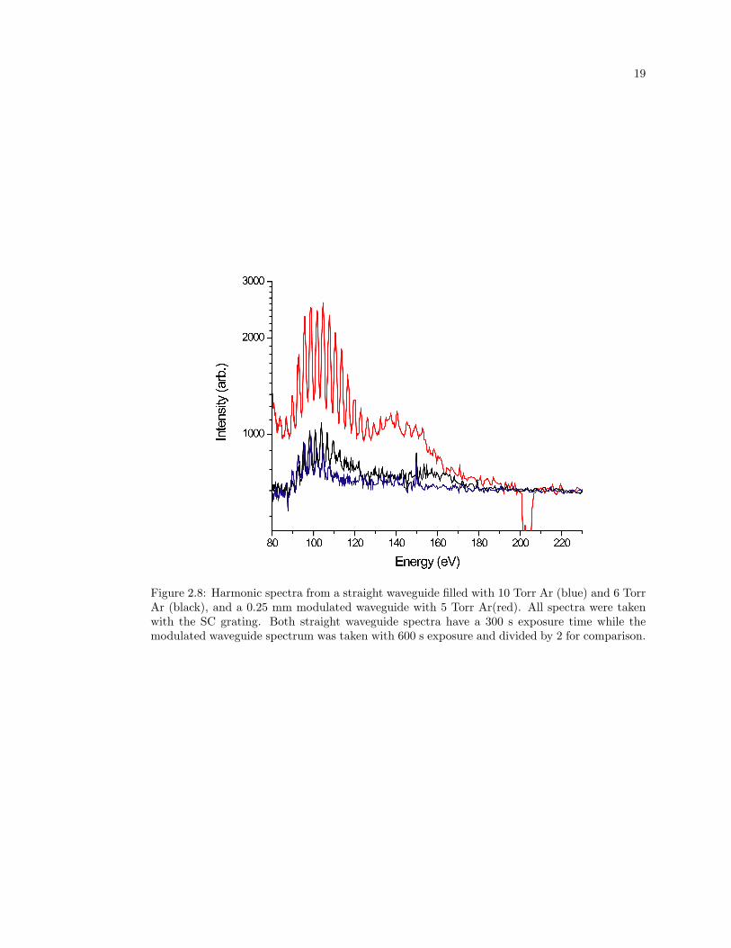
indicating a first order QPM process. Figure 2.8 shows harmonics from straight and modulated

waveguides filled with Ar taken on a different day. Here, the enhancement from QPM is even

more dramatic.

1 0 0 1 2 0 1 4 0 1 6 0 1 8 0 2 0 0 2 2 0 2 4 0

1 0 0 0

1 0 0 0 0

Inten

sity (a

rb.)

E n e r g y ( e V )

Figure 2.6: Harmonic spectra from straight (black), 0.5 mm (blue), and 0.25 mm (red) periodic-ity modulated waveguides filled with 6 Torr neon. The spectra were taken using the SC gratingand a 10 second exposure time.

The gas pressure in the waveguide is an important parameter in these experiments. Figure

2.9 shows harmonic spectra from the three different waveguides at different neon pressures.

Typically, lower gas pressures increase the highest observed harmonic orders. This effect could

be a result of reduced plasma defocusing or absorption, both of which can reduce the intensity

of the driving laser. Fig. 2.9 also plots the flux for three different photon energy ranges as a

function of pressure for the different waveguides. From these plots, it is apparent that there

18

Figure 2.7: Harmonic emission from straight (black) and 0.25 mm (red) modulated waveguidesfilled with 7 Torr Ar. From [31]. The spectra were taken using the SC grating. The exposuretime for the straight waveguide was 300 seconds while for the modulated it was 200 seconds.The spectrum for the modulated waveguide has been multiplied by 1.5 for comparison.

19

Figure 2.8: Harmonic spectra from a straight waveguide filled with 10 Torr Ar (blue) and 6 TorrAr (black), and a 0.25 mm modulated waveguide with 5 Torr Ar(red). All spectra were takenwith the SC grating. Both straight waveguide spectra have a 300 s exposure time while themodulated waveguide spectrum was taken with 600 s exposure and divided by 2 for comparison.

20

is phase matching of higher photon energies in the modulated waveguides while in the straight

waveguide, phase matching is only achieved for the lower energies.

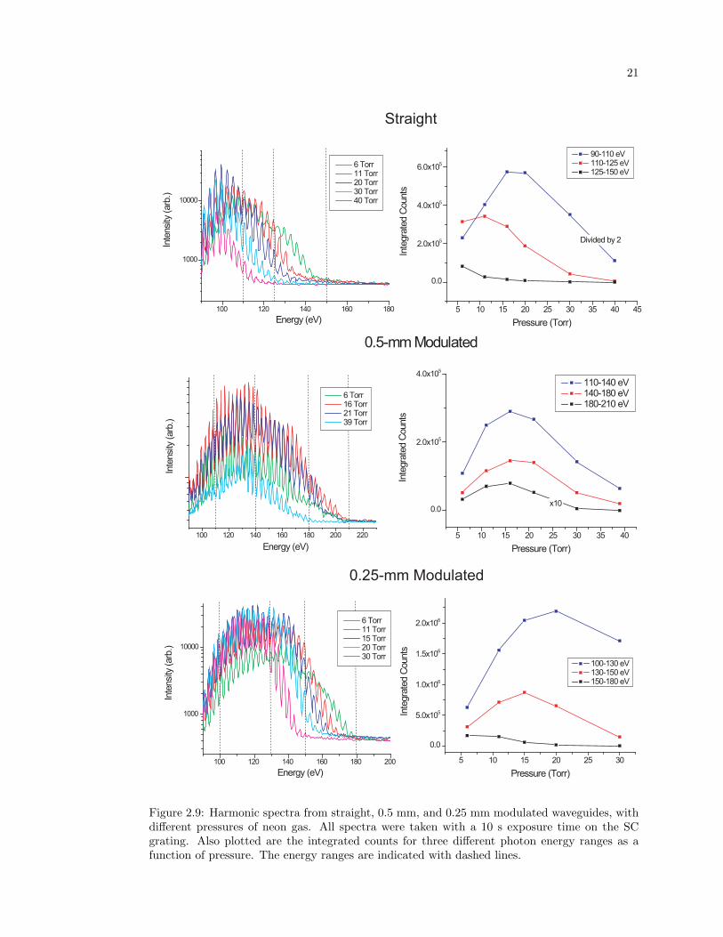
The next series of experiments were done at a higher laser intensity of 1.6 x 1015 W/cm2,

accomplished by using two pump lasers on the second stage of the amplifier giving ∼3 mJ of

pulse energy at the output. The fundamental light was blocked with Ag filters of 0.45 µm

total thickness. Figure 2.10 shows the harmonic emission from 0.25 mm-modulated and straight

waveguides filled with 9 Torr Ne. At these intensities, a simple calculation of the cutoff harmonic

energy, using Eqn. 1.1, yields an expected cutoff of 330 eV. However, the observable harmonic

emission from the straight waveguide (Fig. 2.10 (black curve)) only extends to around 225

eV. In contrast, the harmonic emission from the 0.25 mm modulated waveguide (red curve)

is brighter and extends to significantly higher energies, where the carbon edge at 284 eV is

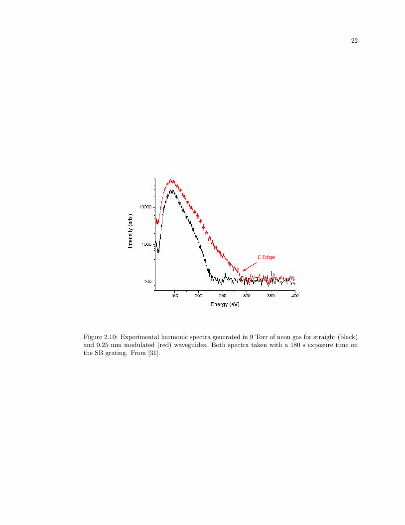
clearly visible. Figure 2.11 shows the harmonic spectra when using helium gas. The modulated

waveguide enhances the harmonic signal over the entire measured spectrum by at least an order

of magnitude, and extends the observable harmonics to 284 eV.

To estimate the amount of phase mismatch in these experiments, the amount of ionization

during the time-window in the pulse that a particular harmonic is generated is calculated using

ADK (Ammosov-Delone-Krainov) tunnelling ionization rates.[3][See Appendix A for details on

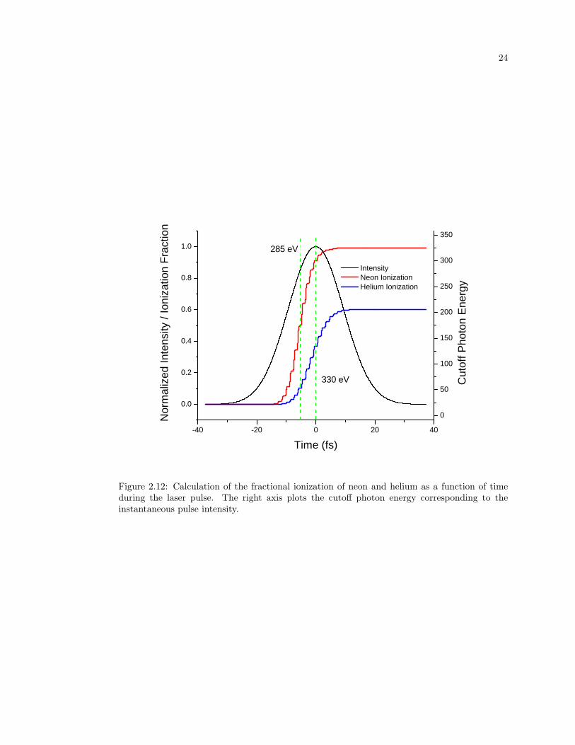
the calculations] Figure 2.12 shows the fractional ionization of neon and helium as a function

of time during the driving pulse for our experimental conditions (pulse duration of 22 fs, peak

intensity of 1.6 x 1015 W/cm2). The amount of ionization at the threshold intensity necessary

to generate 285 eV harmonics is ∼ 50% in neon and ∼ 10% in helium, while at the peak of the

pulse it is ∼ 90% and ∼ 37%. The increasing amount of ionization leads to an increasing phase

mismatch and therefore the dramatic decrease in the flux observed going to higher harmonic

energies. Using the expression in Eq. 2.8, which is valid at high ionization levels, the phase

mismatch for the 183rd harmonic order at the C edge (284 eV) in Ne is calculated to be ∆k ∼

77,000 m−1, assuming 50 % ionization. The effective wavevector for first-order QPM for a

modulation period of 0.25 mm is K1 ∼ 25,000 m−1. Again, the harmonic signal will be enhanced

21

100 120 140 160 180

1000

10000

Inte

nsity

(arb

.)

Energy (eV)

6 Torr 11 Torr 20 Torr 30 Torr 40 Torr

Straight

100 120 140 160 180 200 220

Inte

nsity

(arb

.)

Energy (eV)

6 Torr 16 Torr 21 Torr 39 Torr

0.5-mm Modulated

5 10 15 20 25 30 35 40

0.0

2.0x105

4.0x105

Inte

grat

ed C

ount

s

Pressure (Torr)

110-140 eV 140-180 eV 180-210 eV

x10

5 10 15 20 25 30 35 40 45

0.0

2.0x105

4.0x105

6.0x105

Inte

grat

ed C

ount

s

Pressure (Torr)

90-110 eV 110-125 eV 125-150 eV

Divided by 2

100 120 140 160 180 200

1000

10000

Inte

nsity

(arb

.)

Energy (eV)

6 Torr 11 Torr 15 Torr 20 Torr 30 Torr

0.25-mm Modulated

5 10 15 20 25 30

0.0

5.0x105

1.0x106

1.5x106

2.0x106

Inte

grat

ed C

ount

s

Pressure (Torr)

100-130 eV 130-150 eV 150-180 eV

Figure 2.9: Harmonic spectra from straight, 0.5 mm, and 0.25 mm modulated waveguides, withdifferent pressures of neon gas. All spectra were taken with a 10 s exposure time on the SCgrating. Also plotted are the integrated counts for three different photon energy ranges as afunction of pressure. The energy ranges are indicated with dashed lines.

22

C Edge

Figure 2.10: Experimental harmonic spectra generated in 9 Torr of neon gas for straight (black)and 0.25 mm modulated (red) waveguides. Both spectra taken with a 180 s exposure time onthe SB grating. From [31].

23

1 5 0 2 0 0 2 5 0 3 0 0 3 5 0

1 0 0 0

1 0 0 0 0

Inten

sity (a

rb.)

E n e r g y ( e V )

Figure 2.11: Experimental harmonic spectra generated in helium at 15 Torr using a 0.25 mmmodulated waveguide (black), and at 16 Torr (blue) and 10 Torr (red) using a straight waveguide.All spectra taken with 120 s exposure on SB grating.

24

- 4 0 - 2 0 0 2 0 4 0

0 . 0

0 . 2

0 . 4

0 . 6

0 . 8

1 . 0

0

5 0

1 0 0

1 5 0

2 0 0

2 5 0

3 0 0

3 5 0

3 3 0 e V

Norm

alized

Inten

sity / I

oniza

tion F

ractio

n

T i m e ( f s )

2 8 5 e V I n t e n s i t y N e o n I o n i z a t i o n H e l i u m I o n i z a t i o n

Cutof

f Pho

ton En

ergy

Figure 2.12: Calculation of the fractional ionization of neon and helium as a function of timeduring the laser pulse. The right axis plots the cutoff photon energy corresponding to theinstantaneous pulse intensity.

25

by QPM when Km ≈ ∆k. The greatest enhancement is for m=1 QPM, but there will still be

enhancement of the HHG signal for higher values of m. Thus, for the harmonics in Ne near the

C edge, it is possible to compensate for the large phase mismatch of ∼ 77,000 m−1 by third

order (m=3) QPM. For the harmonics above 225 eV, the phase mismatch is large enough that

the signal can only be observed using a modulated waveguide and is below the noise level for

a straight waveguide. For helium, ∆k ∼ 34,000 m−1 for the 183rd harmonic order at the C

edge, closer to first order QPM. The spectra shown in figures 2.10 and 2.11 illustrate that the

highest observed harmonic orders are not limited by the Ip +3.17Up relation, but by ionization-

induced phase mismatch. The modulated waveguide compensates for this phase mismatch,

making it possible to observe higher harmonics. Although past work observed HHG from He in

the water window, this process was not phase matched and produced significantly lower signal

levels.[15, 70]

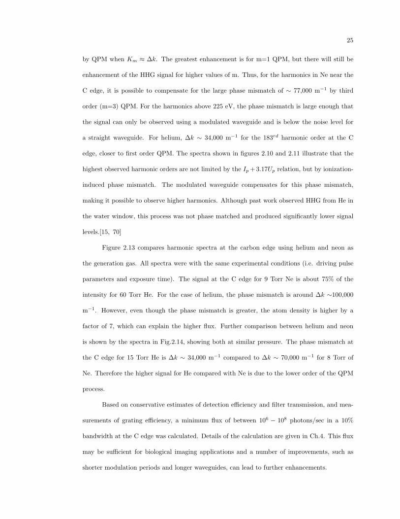
Figure 2.13 compares harmonic spectra at the carbon edge using helium and neon as

the generation gas. All spectra were with the same experimental conditions (i.e. driving pulse

parameters and exposure time). The signal at the C edge for 9 Torr Ne is about 75% of the

intensity for 60 Torr He. For the case of helium, the phase mismatch is around ∆k ∼100,000

m−1. However, even though the phase mismatch is greater, the atom density is higher by a

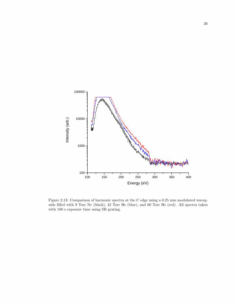
factor of 7, which can explain the higher flux. Further comparison between helium and neon

is shown by the spectra in Fig.2.14, showing both at similar pressure. The phase mismatch at

the C edge for 15 Torr He is ∆k ∼ 34,000 m−1 compared to ∆k ∼ 70,000 m−1 for 8 Torr of

Ne. Therefore the higher signal for He compared with Ne is due to the lower order of the QPM

process.

Based on conservative estimates of detection efficiency and filter transmission, and mea-

surements of grating efficiency, a minimum flux of between 106 − 108 photons/sec in a 10%

bandwidth at the C edge was calculated. Details of the calculation are given in Ch.4. This flux

may be sufficient for biological imaging applications and a number of improvements, such as

shorter modulation periods and longer waveguides, can lead to further enhancements.

26

1 0 0 1 5 0 2 0 0 2 5 0 3 0 0 3 5 0 4 0 01 0 0

1 0 0 0

1 0 0 0 0

1 0 0 0 0 0

Inten

sity (a

rb.)

E n e r g y ( e V )

Figure 2.13: Comparison of harmonic spectra at the C edge using a 0.25 mm modulated waveg-uide filled with 9 Torr Ne (black), 42 Torr He (blue), and 60 Torr He (red). All spectra takenwith 180 s exposure time using SB grating.

27

1 0 0 1 5 0 2 0 0 2 5 0 3 0 0 3 5 0 4 0 0

1 0 0

1 0 0 0

1 0 0 0 0

Inten

sity (a

rb.)

E n e r g y ( e V )

Figure 2.14: Comparison of harmonic spectra from 8 Torr Ne (black) and 15 Torr He (red)using a 0.25 mm modulated waveguide. Both spectra taken with 120 s exposure time using SBgrating.

28

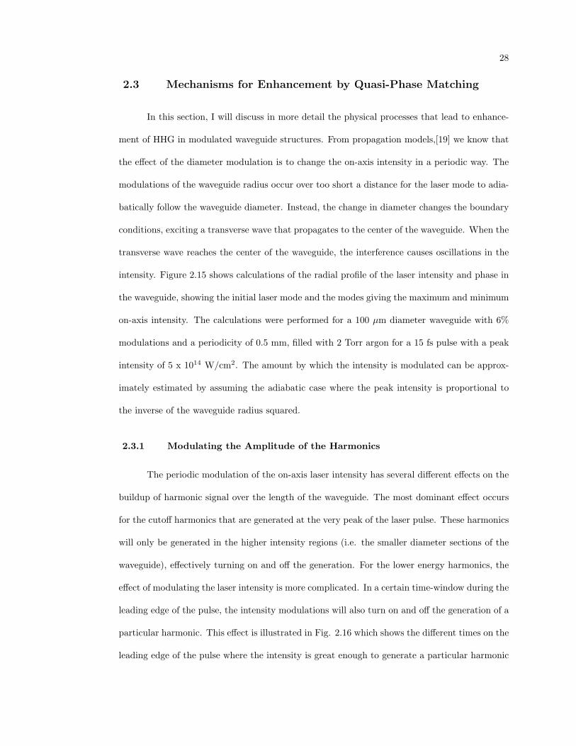
2.3 Mechanisms for Enhancement by Quasi-Phase Matching

In this section, I will discuss in more detail the physical processes that lead to enhance-

ment of HHG in modulated waveguide structures. From propagation models,[19] we know that

the effect of the diameter modulation is to change the on-axis intensity in a periodic way. The

modulations of the waveguide radius occur over too short a distance for the laser mode to adia-

batically follow the waveguide diameter. Instead, the change in diameter changes the boundary

conditions, exciting a transverse wave that propagates to the center of the waveguide. When the

transverse wave reaches the center of the waveguide, the interference causes oscillations in the

intensity. Figure 2.15 shows calculations of the radial profile of the laser intensity and phase in

the waveguide, showing the initial laser mode and the modes giving the maximum and minimum

on-axis intensity. The calculations were performed for a 100 µm diameter waveguide with 6%

modulations and a periodicity of 0.5 mm, filled with 2 Torr argon for a 15 fs pulse with a peak

intensity of 5 x 1014 W/cm2. The amount by which the intensity is modulated can be approx-

imately estimated by assuming the adiabatic case where the peak intensity is proportional to

the inverse of the waveguide radius squared.

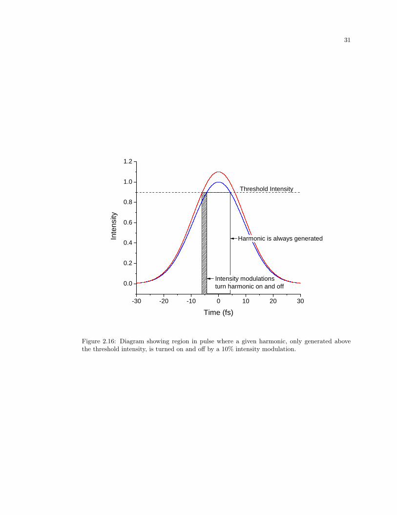
2.3.1 Modulating the Amplitude of the Harmonics

The periodic modulation of the on-axis laser intensity has several different effects on the

buildup of harmonic signal over the length of the waveguide. The most dominant effect occurs

for the cutoff harmonics that are generated at the very peak of the laser pulse. These harmonics

will only be generated in the higher intensity regions (i.e. the smaller diameter sections of the

waveguide), effectively turning on and off the generation. For the lower energy harmonics, the

effect of modulating the laser intensity is more complicated. In a certain time-window during the

leading edge of the pulse, the intensity modulations will also turn on and off the generation of a

particular harmonic. This effect is illustrated in Fig. 2.16 which shows the different times on the

leading edge of the pulse where the intensity is great enough to generate a particular harmonic

29

(a)

(b)

(c)

Figure 2.15: Calculations of the radial profile of the intensity (red curve) and phase (greencurve) of the laser inside the modulated waveguide. The three frames correspond to: a. theinitial mode, b. the mode giving the maximum on-axis intensity and c. the minimum on-axisintensity. From Ivan Christov.

30

when the pulse peak intensity changes by 10%. It is interesting to note that for increasing

harmonic orders, i.e. higher threshold intensities, the duration of this time-window increases.

The expected enhancement due to modulating the harmonic amplitude can be modelled

using the simple formalism described previously. Evaluating equations 2.4 and 2.5 gives an

expression for the amplitude of the harmonic field as a function of propagation length, L:[27]

Eq ∝ ideffEnωLe−i(∆k−Km)L/2Gm

Sin[(∆k −Km)L/2](∆k −Km)L/2

, (2.9)

where the integral is dominated by the term in the sum for which ∆k ≈ Km. The quasi-

phase matching bandwidth is the same as the normal phase matching bandwidth shifted by the

effective wavevector, Km, so that using a longer medium with more modulated sections will

narrow the bandwidth. In the case of periodically poled materials where the phase relation

between the fundamental and harmonic is adjusted by 180 degrees every coherence length, the

nonlinear coefficient can be expressed as a square wave function, oscillating between +1 and -1

every coherence length, with the coefficients given by:[13]

Gm = (2/mπ)Sin(mπ/2) (2.10)

In our case, the enhancement in harmonic field is half that for the case described above since

we only enhance the signal every other coherence length. For our case with perfect quasi-phase

matching (i.e. Km = ∆k), the enhancement is:

Iq ∝ (deffEnω)2(1/mπ)2L2 (2.11)

The enhancement in harmonic intensity is reduced by a factor of (1/mπ)2 compared to the case

of no phase mismatch. The greatest enhancement will be from m=1 quasi-phase matching and

will decrease for higher values of m.

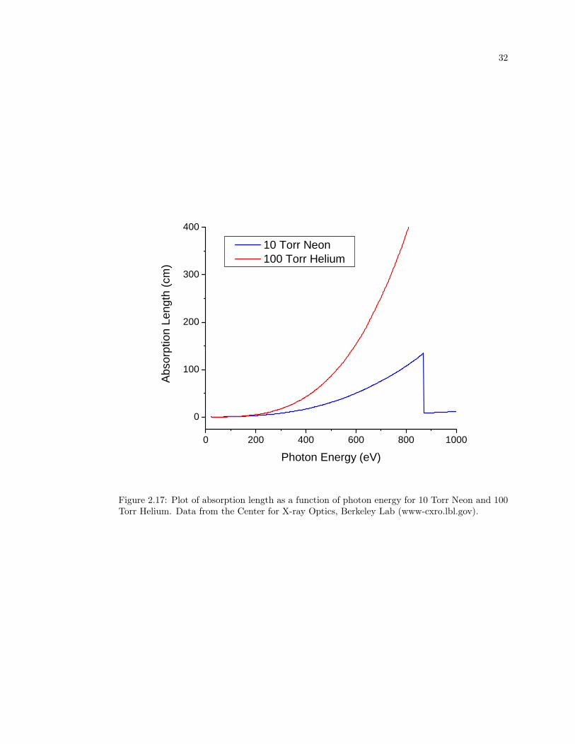
The maximum enhancement of HHG that can be achieved by quasi-phase matching de-

pends upon how strongly the harmonic light is absorbed by the generation gas. Fortunately,

going to higher photon energies, the amount of absorption by the gas decreases significantly.

Figure 2.17 plots the absorption length, Labs, as a function of photon energy for Ne and He

31

- 3 0 - 2 0 - 1 0 0 1 0 2 0 3 0

0 . 0

0 . 2

0 . 4

0 . 6

0 . 8

1 . 0

1 . 2

H a r m o n i c i s a l w a y s g e n e r a t e dInten

sity

T i m e ( f s )

I n t e n s i t y m o d u l a t i o n st u r n h a r m o n i c o n a n d o f f

T h r e s h o l d I n t e n s i t y

Figure 2.16: Diagram showing region in pulse where a given harmonic, only generated abovethe threshold intensity, is turned on and off by a 10% intensity modulation.

32

0 2 0 0 4 0 0 6 0 0 8 0 0 1 0 0 00

1 0 0

2 0 0

3 0 0

4 0 0

Abso

rption

Leng

th (cm

)

P h o t o n E n e r g y ( e V )

1 0 T o r r N e o n 1 0 0 T o r r H e l i u m

Figure 2.17: Plot of absorption length as a function of photon energy for 10 Torr Neon and 100Torr Helium. Data from the Center for X-ray Optics, Berkeley Lab (www-cxro.lbl.gov).

33

gases. For higher photon energies, at and above the C-edge (284 eV), the absorption length

dramatically increases reaching several meters in 100 Torr helium. For quasi-phase matching,

the optimal signal is obtained at the gas pressure where the m=1 quasi-phase matching condi-

tion is met. Previous calculations have shown that the phase matched flux is optimized when

the medium length is > 3Labs and it saturates at around 10Labs.[21] Under our typical exper-

imental conditions, m=1 quasi-phase matching of the harmonics at the C-edge in helium gas

is achieved at a pressure of 9 Torr (for a 0.25 mm modulated waveguide) and the absorption

length at this pressure is Labs = 1.64 m. Therefore, by simple estimates, the maximum sig-

nal enhancement possible would be ∼ (1/mπ)2(10Labs/Lcoh)2(1/e)10 ∼ 80, 000. With shorter

modulation periods, the same signal enhancement could be obtained at a higher pressure and

a shorter waveguide. One issue with using such a long waveguide is the power loss associated

with the fundamental mode propagation. The attenuation constant for the EH11 mode for 800

nm light and a waveguide radius of 75 µm is α = 0.323 m−1.[50] Also, the dispersion of the

waveguide can stretch the pulse in time. The propagation length that would approximately

double the pulse duration is ∼ 14 m.[Note: This calculation is detailed in Ch. 5] Both effects

will reduce the peak intensity of the pulse as it is propagating down the waveguide, preventing

quasi-phase matching over the entire length. One elegant solution to this problem, mentioned

by Ivan Christov in Ref. [19], would be to use a tapered waveguide with a decreasing radius

along its length, maintaining the same on-axis intensity throughout.

2.3.2 Grating-Assisted Phase Matching

Typically quasi-phase matching is implemented by a modulation of the nonlinear coeffi-

cient, however, it is also possible to achieve an enhancement from quasi-phase matching by mod-

ulating the linear optical properties. This process is termed grating-assisted phase matching.[27]

Modulation of the laser intensity in the waveguide results in a modulation in the value of the

phase mismatch, ∆k, along the waveguide from the changing plasma dispersion. The modula-

tion in intensity directly modulates the ionization fraction. For a sinusoidal modulation in the

34

intensity, the plasma contribution to the phase mismatch can be expressed approximately as,

∆kplasma(z) = PNatmreqλ(η + δη cos(2πz/Λ)), (2.12)

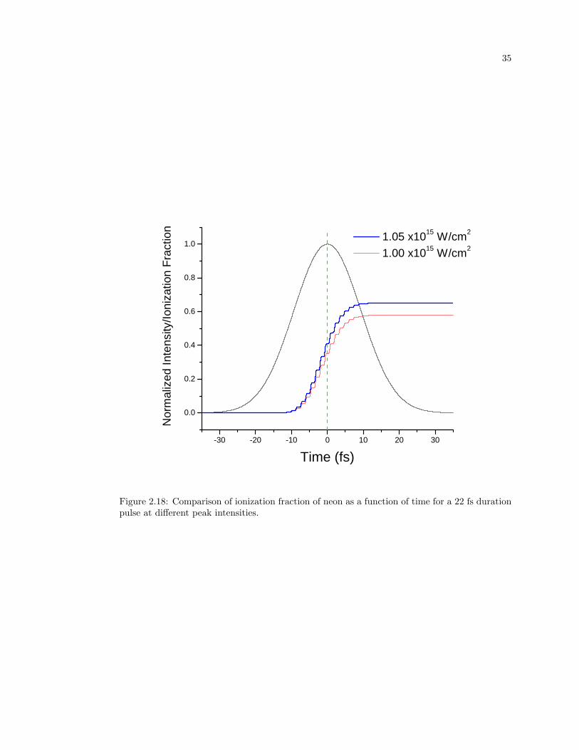
where δη is the change in ionization and Λ is the period of the waveguide modulations. To get

an idea of the amount by which the ionization can change, Fig. 2.18 shows the ionization as a

function of time for two different laser intensities calculated from ADK ionization rates. At the

peak of the pulse, the ionization fraction is 0.35 for an intensity of 1015 W/cm2 and 0.41 when

the intensity is increased by 5%. The value of ∆kplasma therefore changes by 16%. Dramatic

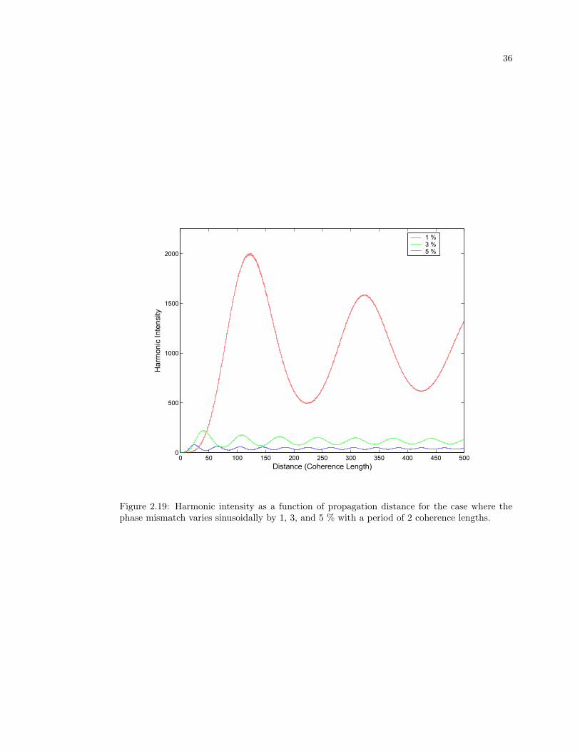
enhancement of the harmonic signal can be obtained if the phase mismatch varies sinusoidally

with a period of twice the coherence length of the average value of ∆k. Mathematically, the

phase mismatch is expressed by:

∆k =π

Lc(1 + α sin(

πz

Lc)), (2.13)

where α is the fractional change. Figure 2.19 shows the calculated harmonic intensity for a

sinusoidally varying phase mismatch for variations of 1, 3, and 5 %. It is interesting that

the smaller variation can give more signal enhancement, but only over a longer propagation

distance. The largest enhancement for a 1 % modulation occurs for a propagation distance of

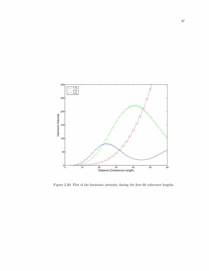
∼ 125 coherence lengths and gives a factor of 2000. Figure 2.20 shows the harmonic signal for

the first 60 coherence lengths. At the beginning, the QPM process is working until a certain

distance at which the signal buildup reverses and then oscillates.

These calculations only take into account the effect of ionization, as would be the case if

one could artificially create a longitudinally varying ionization in a straight waveguide. In the

modulated waveguide, however, there is also a spatial phase due to the periodic refocusing of the

fundamental light. The combination of both effects must be taken into account to understand

the amount of enhancement under real experimental conditions.

35

- 3 0 - 2 0 - 1 0 0 1 0 2 0 3 0

0 . 0

0 . 2

0 . 4

0 . 6

0 . 8

1 . 0

Norm

alized

Inten

sity/Io

nizati

on Fr

actio

n

T i m e ( f s )

1 . 0 5 x 1 0 1 5 W / c m 2

1 . 0 0 x 1 0 1 5 W / c m 2

Figure 2.18: Comparison of ionization fraction of neon as a function of time for a 22 fs durationpulse at different peak intensities.

36

0 50 100 150 200 250 300 350 400 450 5000

500

1000

1500

2000

Distance (Coherence Length)

Har

mon

ic In

tens

ity

1 %3 %5 %

Figure 2.19: Harmonic intensity as a function of propagation distance for the case where thephase mismatch varies sinusoidally by 1, 3, and 5 % with a period of 2 coherence lengths.

37

0 10 20 30 40 50 600

50

100

150

200

250

300

Distance (Coherence Length)

Har

mon

ic In

tens

ity

1 %3 %5 %

Figure 2.20: Plot of the harmonic intensity during the first 60 coherence lengths.

38

2.3.3 Intrinsic Phase Effects

Another mechanism for quasi-phase matching arises from the finite time response of the

harmonic generation process, causing an intensity-dependent phase of the emitted harmonics.

The Lewenstein model of HHG, discussed in Ch. 1, describes the phase of the emitted harmonics

as the phase the electron wavefunction acquires from when the atom is ionized to the time it

recombines. Due to this intrinsic phase, modulation of the intensity of the driving laser can

periodically adjust the phase relationship between the harmonics and the fundamental laser.

The full expression for the harmonic phase relative to the fundamental is given by:[9]

Φ = qωtf − S(t0, tf )/h̄, (2.14)

where q is the harmonic order, ω is the fundamental laser frequency and S(t0, tf ) is the quasi-

classical action of the electron from the time the atom is ionized, t0, to when the electron

recombines, tf . The quasi-classical action is given by the expression:

S(t0, tf ) =∫ tf

t0

(p2

2m+ Ip)dt (2.15)

where p is the electron momentum, m is the electron mass, and Ip is the ionization potential

of the atom. Previous theoretical work has solved for the phase of the harmonics using the

method of stationary action.[47, 29] Here, I will follow a slightly different approach, solving the

integral in Eqn. 2.15 numerically over the classical trajectory of the free electron to determine

the harmonic phase.

The classical trajectory of a free electron in the laser field is given by:

mdv

dt= −eE(t). (2.16)

Making the assumption of a monochromatic laser field: E(t) = E0Cos(ωt), the equations of

motion for the electron are:

v(φ, φ0) =−eE0

mω(Sinφ− Sinφ0) (2.17)

and

x(φ, φ0) =eE0

mω2(Cosφ− Cosφ0 − Sinφ0(φ− φ0)), (2.18)

39

where φ = ωt and φ0 = ωt0 is the phase in the laser cycle when the atom is ionized, termed the

release phase. From the equations of motion, we can solve for the phase, φf , when the electron

returns to the position of the ion. This return phase as a function of the release phase is plotted

in Fig. 2.21. It is then straightforward to solve for the electron’s velocity, and therefore its

kinetic energy, when it re-encounters the ion. Fig. 2.22 plots the kinetic energy as a function of

the electron’s release phase. From Fig. 2.22 it is evident that for the harmonics at the cutoff,

there is only one classical trajectory; however, for the plateau harmonics, there are two different

trajectories (short and long) with the same return kinetic energy. For the short trajectories,

the electron is released at a phase > 18 degrees, and re-encounters the ion in less than half an

optical cycle. The duration of the long trajectories, however, is almost a full optical cycle and

therefore the electron acquires more phase.

Combining equations 2.15 and 2.17 gives the following expression for the intrinsic phase

of the harmonics due to the phase that the electron acquires in its trajectory as a function of

the release phase, φ0, and the return phase φf :

φintrinsic =Ip

h̄ω(φf − φ0) +

2Up

h̄ω

∫ φf

φ0

(Sinφ− Sinφ0)2dφ, (2.19)

where the definition of the ponderomotive energy, Up = e2E2/4mω2, is used. For the case of very

high harmonic orders where the condition Up >> Ip is met, the first term in Eqn. 2.19 can be

neglected and the electron kinetic energy is approximately equal to the emitted photon energy.

Using this assumption, the intrinsic phase as a function of harmonic energy is calculated, plotted

in Fig. 2.23. To find the harmonic phase relative to the fundamental, it is necessary to include

the first term in Eqn. 2.14. The result for the harmonic phase relative to the fundamental is

shown in Fig. 2.24.

For quasi-phase matching, it is important to know how the harmonic phase changes with

laser intensity. Fig. 2.25 plots the result for the intensity dependence of the harmonic phase for

two different harmonic orders, assuming an 800 nm driving laser and the condition Ip = 0. The

long trajectories have a linear intensity dependence equal to ∼ -23 x 10−14 Radians·cm2/W. The

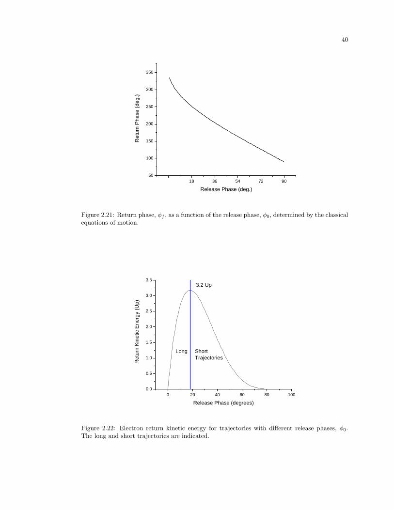
40

1 8 3 6 5 4 7 2 9 05 0

1 0 0

1 5 0

2 0 0

2 5 0

3 0 0

3 5 0

Retur

n Pha

se (d

eg.)

R e l e a s e P h a s e ( d e g . )

Figure 2.21: Return phase, φf , as a function of the release phase, φ0, determined by the classicalequations of motion.

0 2 0 4 0 6 0 8 0 1 0 00 . 0

0 . 5

1 . 0

1 . 5

2 . 0

2 . 5

3 . 0

3 . 5

Retur

n Kine

tic En

ergy (

Up)

R e l e a s e P h a s e ( d e g r e e s )

S h o r tT r a j e c t o r i e s

L o n g

3 . 2 U p

Figure 2.22: Electron return kinetic energy for trajectories with different release phases, φ0.The long and short trajectories are indicated.

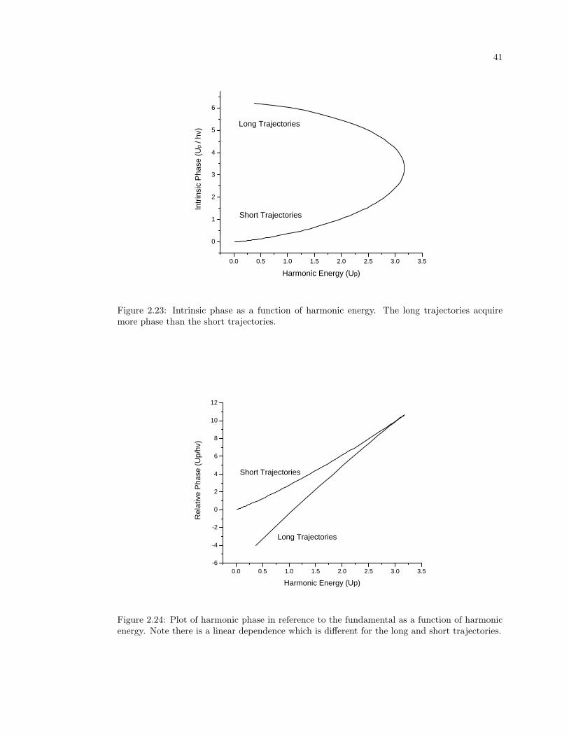
41

0 . 0 0 . 5 1 . 0 1 . 5 2 . 0 2 . 5 3 . 0 3 . 5

0

1

2

3

4

5

6

S h o r t T r a j e c t o r i e sIntrin

sic Ph

ase (

Up / h

v)

H a r m o n i c E n e r g y ( U p )

L o n g T r a j e c t o r i e s

Figure 2.23: Intrinsic phase as a function of harmonic energy. The long trajectories acquiremore phase than the short trajectories.

0 . 0 0 . 5 1 . 0 1 . 5 2 . 0 2 . 5 3 . 0 3 . 5- 6

- 4

- 2

0

2

4

6

8

1 0

1 2

Relat

ive Ph

ase (

Up/hv

)

H a r m o n i c E n e r g y ( U p )

L o n g T r a j e c t o r i e s

S h o r t T r a j e c t o r i e s

Figure 2.24: Plot of harmonic phase in reference to the fundamental as a function of harmonicenergy. Note there is a linear dependence which is different for the long and short trajectories.

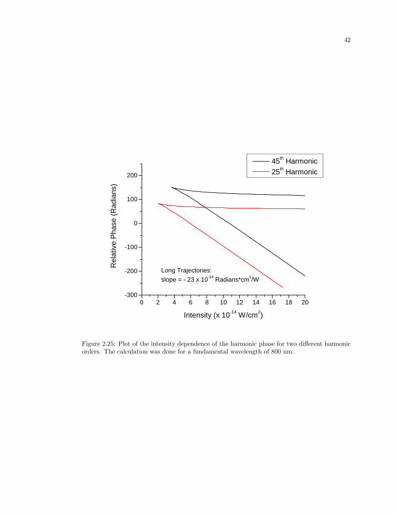
42

0 2 4 6 8 1 0 1 2 1 4 1 6 1 8 2 0- 3 0 0

- 2 0 0

- 1 0 0

0

1 0 0

2 0 0

Relat

ive Ph

ase (

Radia

ns)

I n t e n s i t y ( x 1 0 - 1 4 W / c m 2 )

4 5 t h H a r m o n i c 2 5 t h H a r m o n i c

L o n g T r a j e c t o r i e s :s l o p e = - 2 3 x 1 0 - 1 4 R a d i a n s * c m 2 / W

Figure 2.25: Plot of the intensity dependence of the harmonic phase for two different harmonicorders. The calculation was done for a fundamental wavelength of 800 nm.

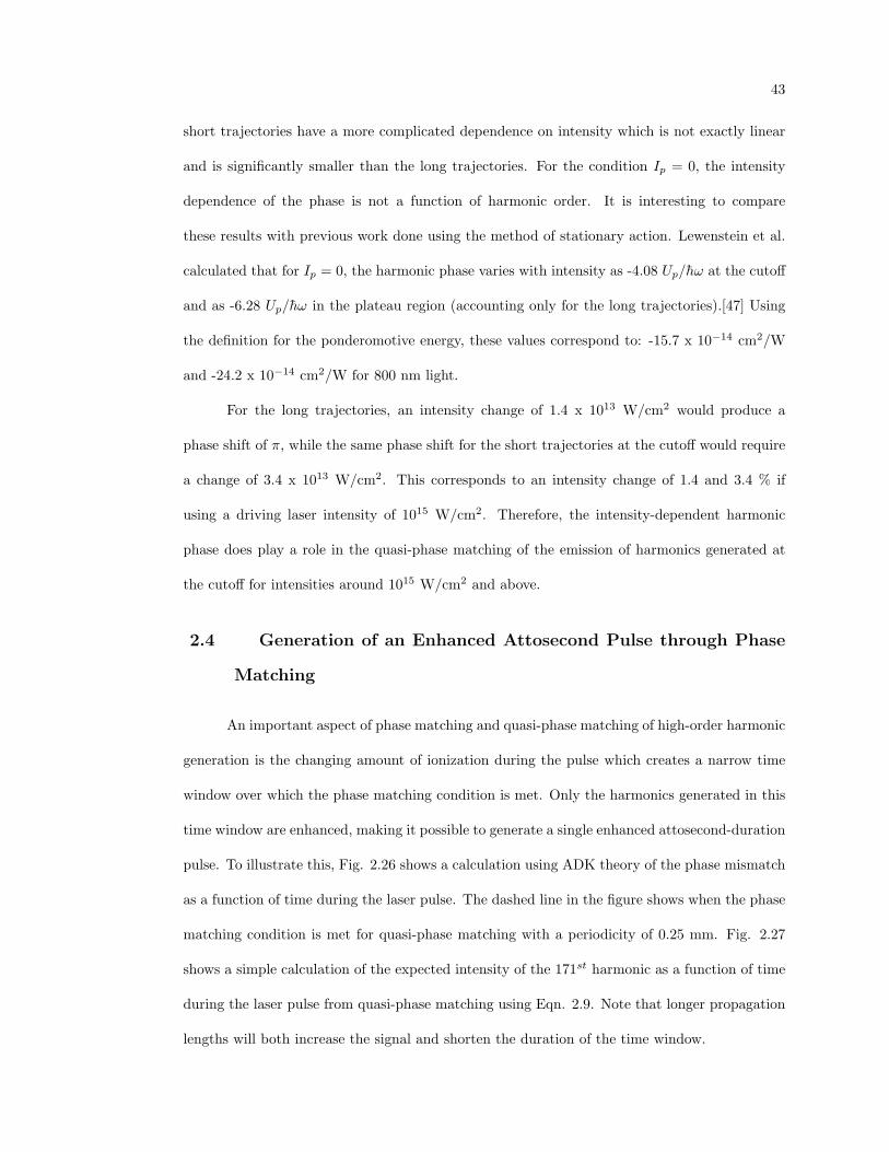
43

short trajectories have a more complicated dependence on intensity which is not exactly linear

and is significantly smaller than the long trajectories. For the condition Ip = 0, the intensity

dependence of the phase is not a function of harmonic order. It is interesting to compare

these results with previous work done using the method of stationary action. Lewenstein et al.

calculated that for Ip = 0, the harmonic phase varies with intensity as -4.08 Up/h̄ω at the cutoff

and as -6.28 Up/h̄ω in the plateau region (accounting only for the long trajectories).[47] Using

the definition for the ponderomotive energy, these values correspond to: -15.7 x 10−14 cm2/W

and -24.2 x 10−14 cm2/W for 800 nm light.

For the long trajectories, an intensity change of 1.4 x 1013 W/cm2 would produce a

phase shift of π, while the same phase shift for the short trajectories at the cutoff would require

a change of 3.4 x 1013 W/cm2. This corresponds to an intensity change of 1.4 and 3.4 % if

using a driving laser intensity of 1015 W/cm2. Therefore, the intensity-dependent harmonic

phase does play a role in the quasi-phase matching of the emission of harmonics generated at

the cutoff for intensities around 1015 W/cm2 and above.

2.4 Generation of an Enhanced Attosecond Pulse through Phase

Matching

An important aspect of phase matching and quasi-phase matching of high-order harmonic

generation is the changing amount of ionization during the pulse which creates a narrow time

window over which the phase matching condition is met. Only the harmonics generated in this

time window are enhanced, making it possible to generate a single enhanced attosecond-duration

pulse. To illustrate this, Fig. 2.26 shows a calculation using ADK theory of the phase mismatch

as a function of time during the laser pulse. The dashed line in the figure shows when the phase

matching condition is met for quasi-phase matching with a periodicity of 0.25 mm. Fig. 2.27

shows a simple calculation of the expected intensity of the 171st harmonic as a function of time

during the laser pulse from quasi-phase matching using Eqn. 2.9. Note that longer propagation

lengths will both increase the signal and shorten the duration of the time window.

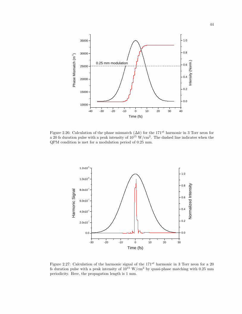
44

- 4 0 - 3 0 - 2 0 - 1 0 0 1 0 2 0 3 0 4 01 0 0 0 0

1 5 0 0 0

2 0 0 0 0

2 5 0 0 0

3 0 0 0 0

3 5 0 0 0

0 . 0

0 . 2

0 . 4

0 . 6

0 . 8

1 . 0

Phas

e Mism

atch (

m-1 )

T i m e ( f s )

0 . 2 5 m m m o d u l a t i o n

Inten

sity (N

orm.)

Figure 2.26: Calculation of the phase mismatch (∆k) for the 171st harmonic in 3 Torr neon fora 20 fs duration pulse with a peak intensity of 1015 W/cm2. The dashed line indicates when theQPM condition is met for a modulation period of 0.25 mm.

- 3 0 - 2 0 - 1 0 0 1 0 2 0 3 0

0 . 0

2 . 0 x 1 0 - 7

4 . 0 x 1 0 - 7

6 . 0 x 1 0 - 7

8 . 0 x 1 0 - 7

1 . 0 x 1 0 - 6

1 . 2 x 1 0 - 6

0 . 0

0 . 2

0 . 4

0 . 6

0 . 8

1 . 0

Harm

onic S

ignal

T i m e ( f s )

Norm

alized

Inten

sity

Figure 2.27: Calculation of the harmonic signal of the 171st harmonic in 3 Torr neon for a 20fs duration pulse with a peak intensity of 1015 W/cm2 by quasi-phase matching with 0.25 mmperiodicity. Here, the propagation length is 1 mm.

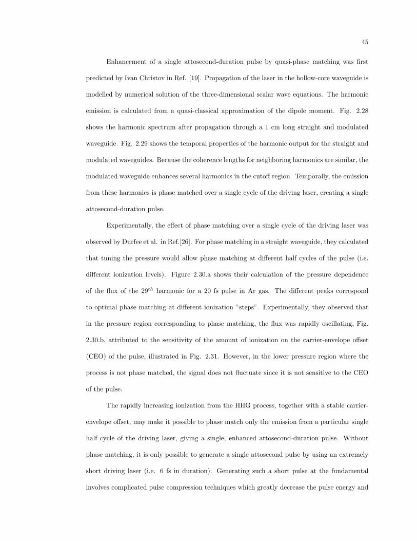
45

Enhancement of a single attosecond-duration pulse by quasi-phase matching was first

predicted by Ivan Christov in Ref. [19]. Propagation of the laser in the hollow-core waveguide is

modelled by numerical solution of the three-dimensional scalar wave equations. The harmonic

emission is calculated from a quasi-classical approximation of the dipole moment. Fig. 2.28

shows the harmonic spectrum after propagation through a 1 cm long straight and modulated

waveguide. Fig. 2.29 shows the temporal properties of the harmonic output for the straight and

modulated waveguides. Because the coherence lengths for neighboring harmonics are similar, the

modulated waveguide enhances several harmonics in the cutoff region. Temporally, the emission

from these harmonics is phase matched over a single cycle of the driving laser, creating a single

attosecond-duration pulse.

Experimentally, the effect of phase matching over a single cycle of the driving laser was

observed by Durfee et al. in Ref.[26]. For phase matching in a straight waveguide, they calculated

that tuning the pressure would allow phase matching at different half cycles of the pulse (i.e.

different ionization levels). Figure 2.30.a shows their calculation of the pressure dependence

of the flux of the 29th harmonic for a 20 fs pulse in Ar gas. The different peaks correspond

to optimal phase matching at different ionization ”steps”. Experimentally, they observed that

in the pressure region corresponding to phase matching, the flux was rapidly oscillating, Fig.

2.30.b, attributed to the sensitivity of the amount of ionization on the carrier-envelope offset

(CEO) of the pulse, illustrated in Fig. 2.31. However, in the lower pressure region where the

process is not phase matched, the signal does not fluctuate since it is not sensitive to the CEO

of the pulse.

The rapidly increasing ionization from the HHG process, together with a stable carrier-

envelope offset, may make it possible to phase match only the emission from a particular single

half cycle of the driving laser, giving a single, enhanced attosecond-duration pulse. Without

phase matching, it is only possible to generate a single attosecond pulse by using an extremely

short driving laser (i.e. 6 fs in duration). Generating such a short pulse at the fundamental

involves complicated pulse compression techniques which greatly decrease the pulse energy and

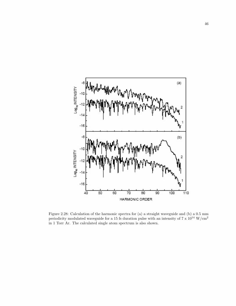
46

Figure 2.28: Calculation of the harmonic spectra for (a) a straight waveguide and (b) a 0.5 mmperiodicity modulated waveguide for a 15 fs duration pulse with an intensity of 7 x 1014 W/cm2

in 1 Torr Ar. The calculated single atom spectrum is also shown.

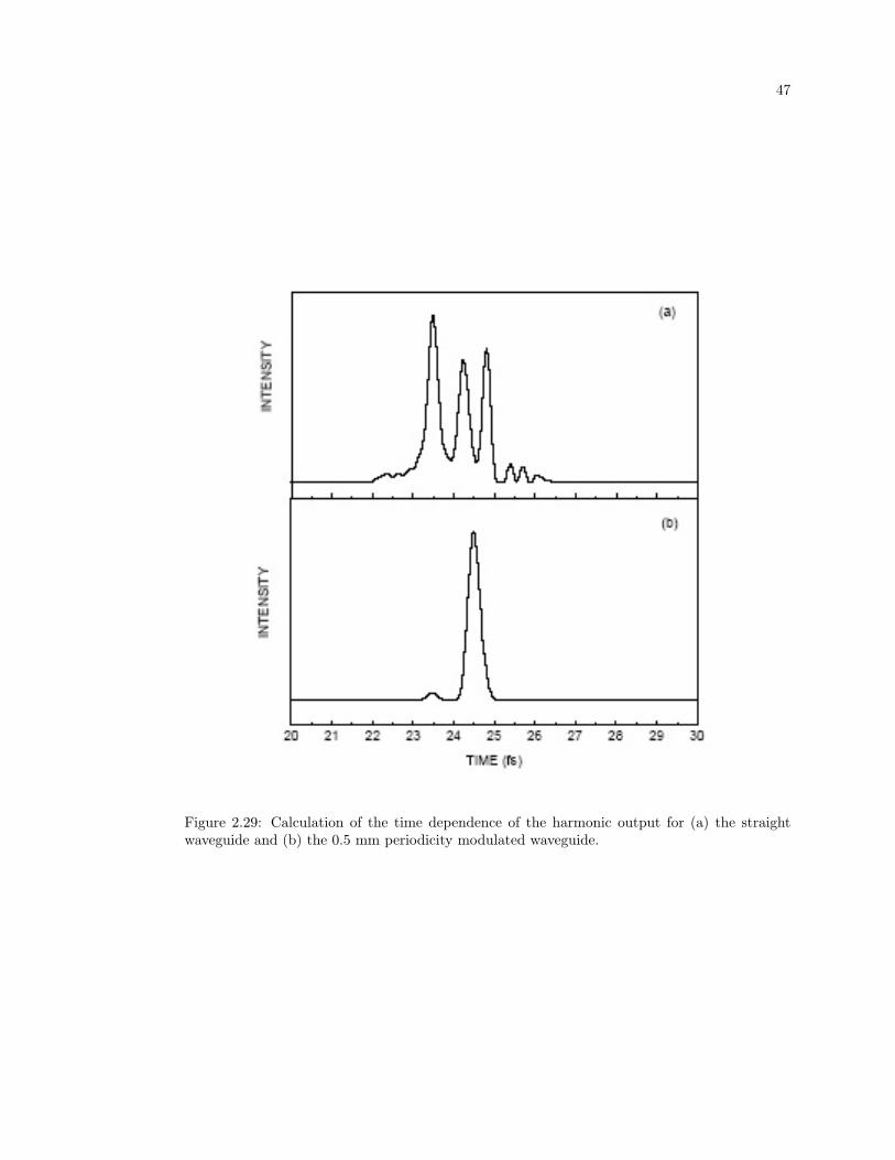
47

Figure 2.29: Calculation of the time dependence of the harmonic output for (a) the straightwaveguide and (b) the 0.5 mm periodicity modulated waveguide.

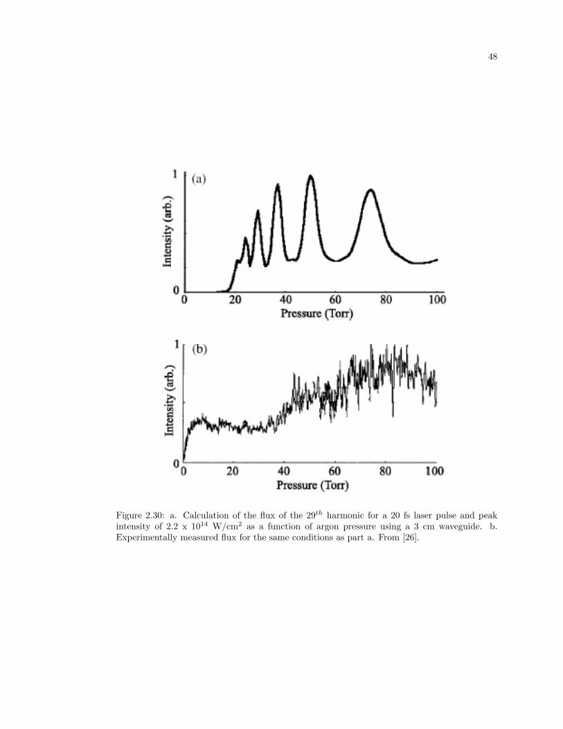
48

Figure 2.30: a. Calculation of the flux of the 29th harmonic for a 20 fs laser pulse and peakintensity of 2.2 x 1014 W/cm2 as a function of argon pressure using a 3 cm waveguide. b.Experimentally measured flux for the same conditions as part a. From [26].

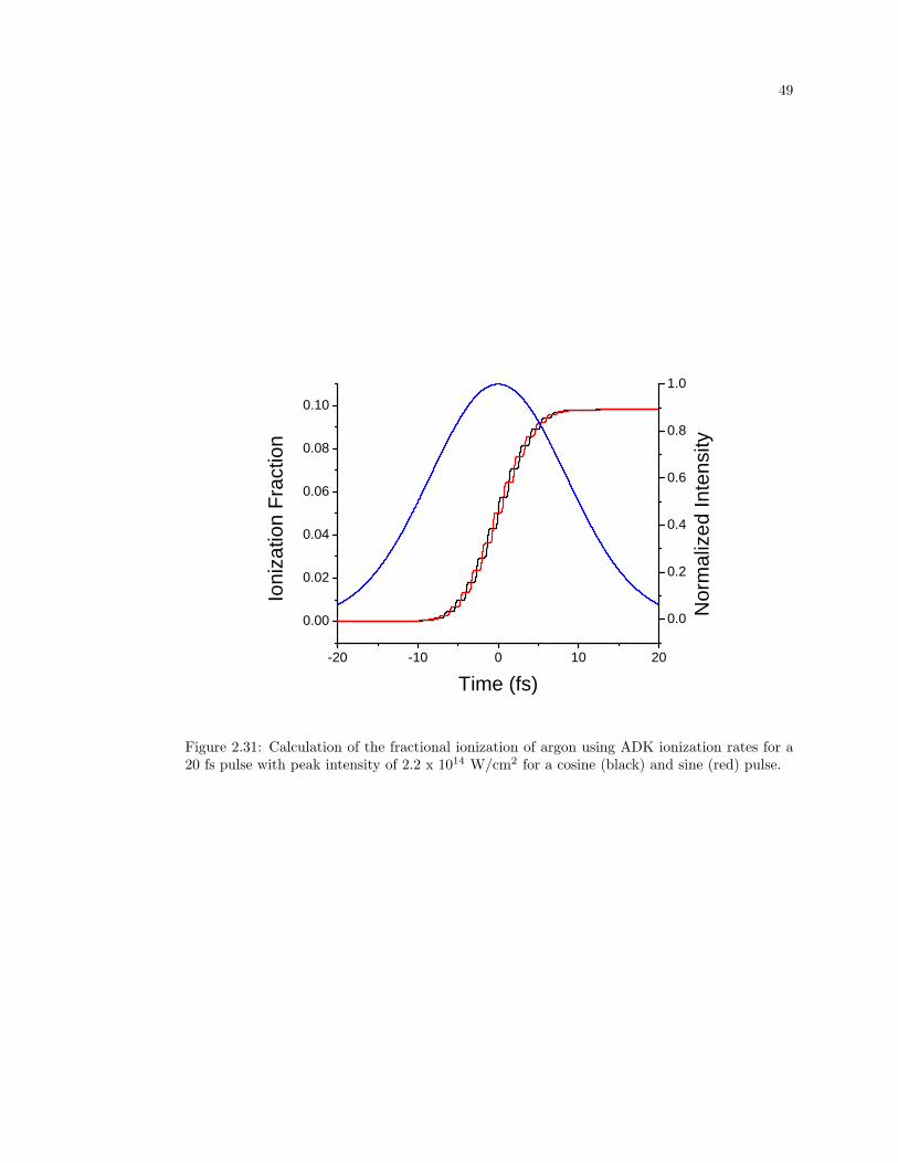
49

- 2 0 - 1 0 0 1 0 2 0

0 . 0 0

0 . 0 2

0 . 0 4

0 . 0 6

0 . 0 8

0 . 1 0

0 . 0

0 . 2

0 . 4

0 . 6

0 . 8

1 . 0

Ioniza

tion F

ractio

n

T i m e ( f s ) No

rmaliz

ed In

tensity

Figure 2.31: Calculation of the fractional ionization of argon using ADK ionization rates for a20 fs pulse with peak intensity of 2.2 x 1014 W/cm2 for a cosine (black) and sine (red) pulse.

50

stability (since they rely on nonlinear processes to broaden the spectrum). Phase matching

in hollow waveguides thus presents a more elegant, stable, and efficient method for attosecond

pulse generation.

Chapter 3

High Harmonic Generation from Ions

The highest photon energies obtained from high harmonic generation (HHG) have gener-

ally been limited not by the cutoff rule, but by the detrimental effects of ionization when using

high laser intensities. The resulting plasma can defocus the laser beam,[59] limiting the peak

intensity and therefore Up. It also causes a significant phase velocity mismatch between the driv-

ing laser and the harmonic light, greatly reducing the harmonic signal. Ionization can be kept

to a minimum by using shorter-duration laser pulses or atoms with a large ionization potential,

thus allowing the atoms survive to high laser intensities before ionizing. The highest harmonics

observed to date, at around 950 eV, have been generated using helium,[15, 70, 67] which has

the largest ionization potential of the noble gases. However, helium also has an exceptionally

small effective nonlinearity, which limits the harmonic flux. Larger, multi-electron atoms such as

argon typically generate greater signals, but the highest observable harmonic orders have been

comparatively lower. For example in Ar, photons of greater than 100 eV energy have never been

observed using an 800 nm driving laser,[83, 80] even using very short 7 fs duration pulses[65] or

large pulse energies. In other work, a longer-wavelength driving laser was used to increase the

harmonic emission in Ar to ∼ 150 eV.[68] Using longer wavelengths increases the value of Up for

the same laser intensity, however, this approach also reduces the efficiency of the process since

the electron wavefunction is more delocalized, lowering the probability of recombination.

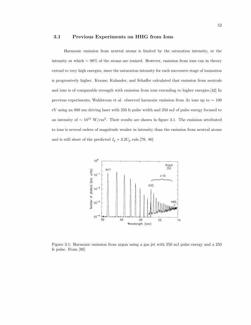
52

3.1 Previous Experiments on HHG from Ions

Harmonic emission from neutral atoms is limited by the saturation intensity, or the

intensity at which ∼ 98% of the atoms are ionized. However, emission from ions can in theory

extend to very high energies, since the saturation intensity for each successive stage of ionization

is progressively higher. Krause, Kulander, and Schaffer calculated that emission from neutrals

and ions is of comparable strength with emission from ions extending to higher energies.[42] In

previous experiments, Wahlstrom et al. observed harmonic emission from Ar ions up to ∼ 100

eV using an 800 nm driving laser with 250 fs pulse width and 250 mJ of pulse energy focused to

an intensity of ∼ 1015 W/cm2. Their results are shown in figure 3.1. The emission attributed

to ions is several orders of magnitude weaker in intensity than the emission from neutral atoms

and is still short of the predicted Ip + 3.2Up rule.[79, 80]

Figure 3.1: Harmonic emission from argon using a gas jet with 250 mJ pulse energy and a 250fs pulse. From [80]

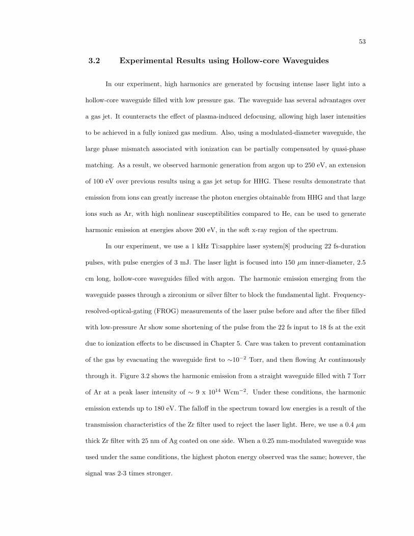
53

3.2 Experimental Results using Hollow-core Waveguides

In our experiment, high harmonics are generated by focusing intense laser light into a

hollow-core waveguide filled with low pressure gas. The waveguide has several advantages over

a gas jet. It counteracts the effect of plasma-induced defocusing, allowing high laser intensities

to be achieved in a fully ionized gas medium. Also, using a modulated-diameter waveguide, the

large phase mismatch associated with ionization can be partially compensated by quasi-phase

matching. As a result, we observed harmonic generation from argon up to 250 eV, an extension

of 100 eV over previous results using a gas jet setup for HHG. These results demonstrate that

emission from ions can greatly increase the photon energies obtainable from HHG and that large

ions such as Ar, with high nonlinear susceptibilities compared to He, can be used to generate

harmonic emission at energies above 200 eV, in the soft x-ray region of the spectrum.

In our experiment, we use a 1 kHz Ti:sapphire laser system[8] producing 22 fs-duration

pulses, with pulse energies of 3 mJ. The laser light is focused into 150 µm inner-diameter, 2.5

cm long, hollow-core waveguides filled with argon. The harmonic emission emerging from the

waveguide passes through a zirconium or silver filter to block the fundamental light. Frequency-

resolved-optical-gating (FROG) measurements of the laser pulse before and after the fiber filled

with low-pressure Ar show some shortening of the pulse from the 22 fs input to 18 fs at the exit

due to ionization effects to be discussed in Chapter 5. Care was taken to prevent contamination

of the gas by evacuating the waveguide first to ∼10−2 Torr, and then flowing Ar continuously

through it. Figure 3.2 shows the harmonic emission from a straight waveguide filled with 7 Torr

of Ar at a peak laser intensity of ∼ 9 x 1014 Wcm−2. Under these conditions, the harmonic

emission extends up to 180 eV. The falloff in the spectrum toward low energies is a result of the

transmission characteristics of the Zr filter used to reject the laser light. Here, we use a 0.4 µm

thick Zr filter with 25 nm of Ag coated on one side. When a 0.25 mm-modulated waveguide was

used under the same conditions, the highest photon energy observed was the same; however, the

signal was 2-3 times stronger.

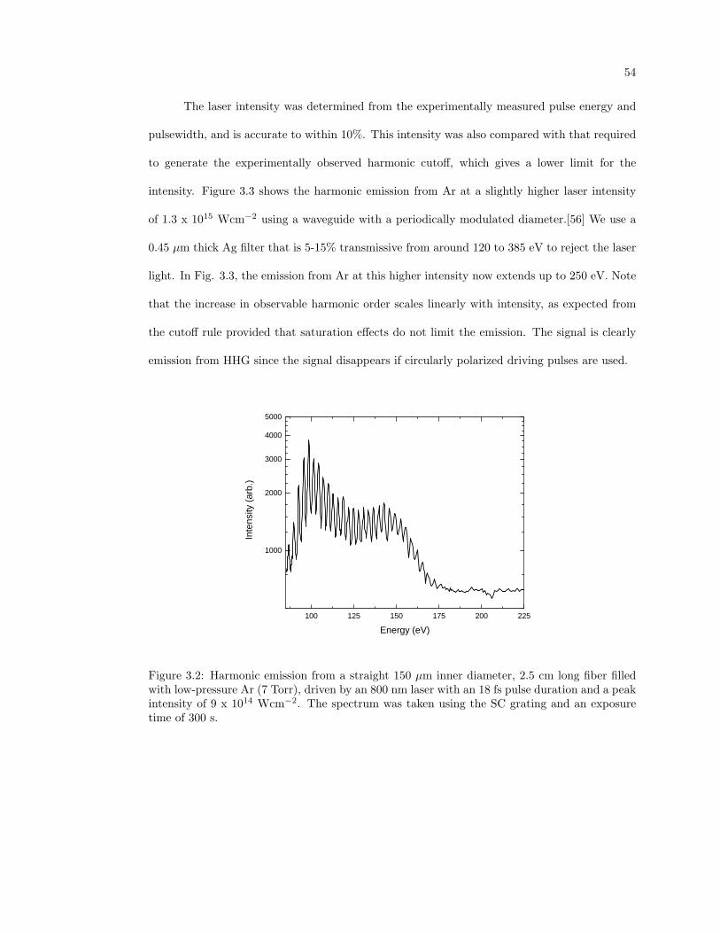
54

The laser intensity was determined from the experimentally measured pulse energy and

pulsewidth, and is accurate to within 10%. This intensity was also compared with that required

to generate the experimentally observed harmonic cutoff, which gives a lower limit for the

intensity. Figure 3.3 shows the harmonic emission from Ar at a slightly higher laser intensity

of 1.3 x 1015 Wcm−2 using a waveguide with a periodically modulated diameter.[56] We use a

0.45 µm thick Ag filter that is 5-15% transmissive from around 120 to 385 eV to reject the laser

light. In Fig. 3.3, the emission from Ar at this higher intensity now extends up to 250 eV. Note

that the increase in observable harmonic order scales linearly with intensity, as expected from

the cutoff rule provided that saturation effects do not limit the emission. The signal is clearly

emission from HHG since the signal disappears if circularly polarized driving pulses are used.

1 0 0 1 2 5 1 5 0 1 7 5 2 0 0 2 2 5

1 0 0 0

2 0 0 0

3 0 0 0

4 0 0 05 0 0 0

Inten

sity (a

rb.)

E n e r g y ( e V )

Figure 3.2: Harmonic emission from a straight 150 µm inner diameter, 2.5 cm long fiber filledwith low-pressure Ar (7 Torr), driven by an 800 nm laser with an 18 fs pulse duration and a peakintensity of 9 x 1014 Wcm−2. The spectrum was taken using the SC grating and an exposuretime of 300 s.

55

100 150 200 250 300 35010

100

1000

10000

Inten

sity (a

rb.)

Energy (eV)

Figure 3.3: Harmonic emission at a higher peak laser intensity of 1.3 x 1015 Wcm−2, using a0.25 mm period modulated waveguide. The spectrum was taken using the SC grating with a600 s exposure time.

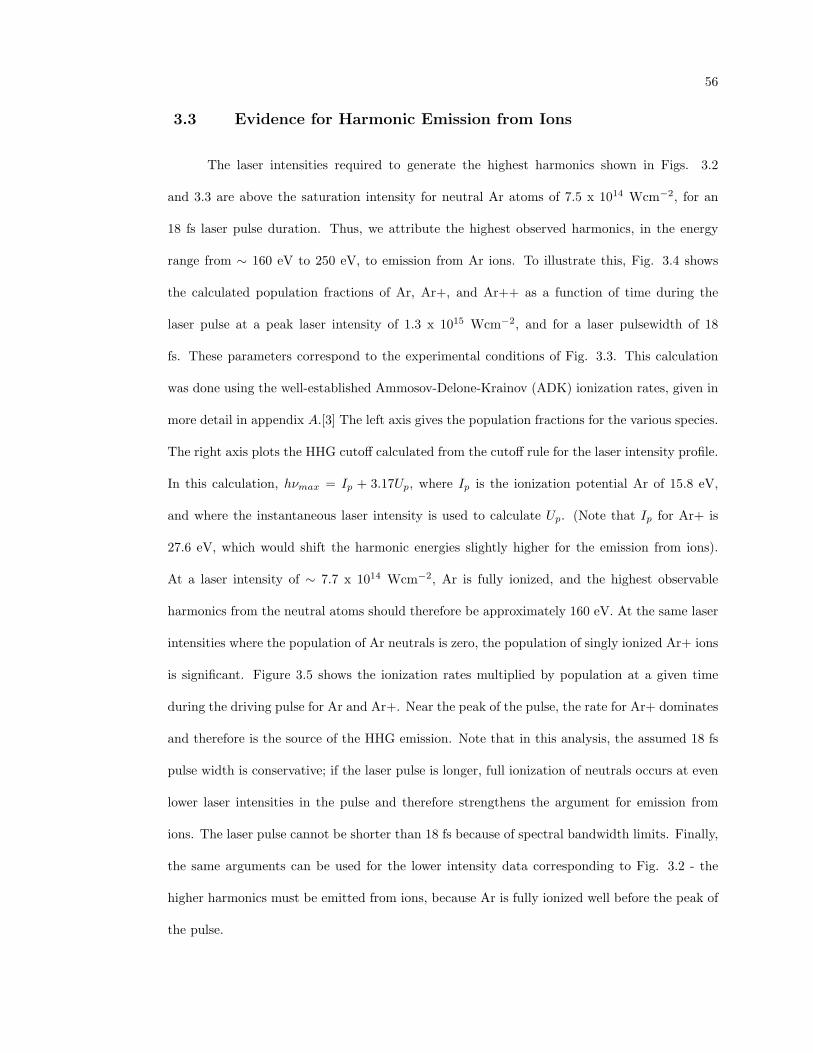
56

3.3 Evidence for Harmonic Emission from Ions

The laser intensities required to generate the highest harmonics shown in Figs. 3.2

and 3.3 are above the saturation intensity for neutral Ar atoms of 7.5 x 1014 Wcm−2, for an

18 fs laser pulse duration. Thus, we attribute the highest observed harmonics, in the energy

range from ∼ 160 eV to 250 eV, to emission from Ar ions. To illustrate this, Fig. 3.4 shows

the calculated population fractions of Ar, Ar+, and Ar++ as a function of time during the

laser pulse at a peak laser intensity of 1.3 x 1015 Wcm−2, and for a laser pulsewidth of 18

fs. These parameters correspond to the experimental conditions of Fig. 3.3. This calculation

was done using the well-established Ammosov-Delone-Krainov (ADK) ionization rates, given in

more detail in appendix A.[3] The left axis gives the population fractions for the various species.

The right axis plots the HHG cutoff calculated from the cutoff rule for the laser intensity profile.

In this calculation, hνmax = Ip + 3.17Up, where Ip is the ionization potential Ar of 15.8 eV,

and where the instantaneous laser intensity is used to calculate Up. (Note that Ip for Ar+ is

27.6 eV, which would shift the harmonic energies slightly higher for the emission from ions).

At a laser intensity of ∼ 7.7 x 1014 Wcm−2, Ar is fully ionized, and the highest observable

harmonics from the neutral atoms should therefore be approximately 160 eV. At the same laser

intensities where the population of Ar neutrals is zero, the population of singly ionized Ar+ ions

is significant. Figure 3.5 shows the ionization rates multiplied by population at a given time

during the driving pulse for Ar and Ar+. Near the peak of the pulse, the rate for Ar+ dominates

and therefore is the source of the HHG emission. Note that in this analysis, the assumed 18 fs

pulse width is conservative; if the laser pulse is longer, full ionization of neutrals occurs at even

lower laser intensities in the pulse and therefore strengthens the argument for emission from

ions. The laser pulse cannot be shorter than 18 fs because of spectral bandwidth limits. Finally,

the same arguments can be used for the lower intensity data corresponding to Fig. 3.2 - the

higher harmonics must be emitted from ions, because Ar is fully ionized well before the peak of

the pulse.

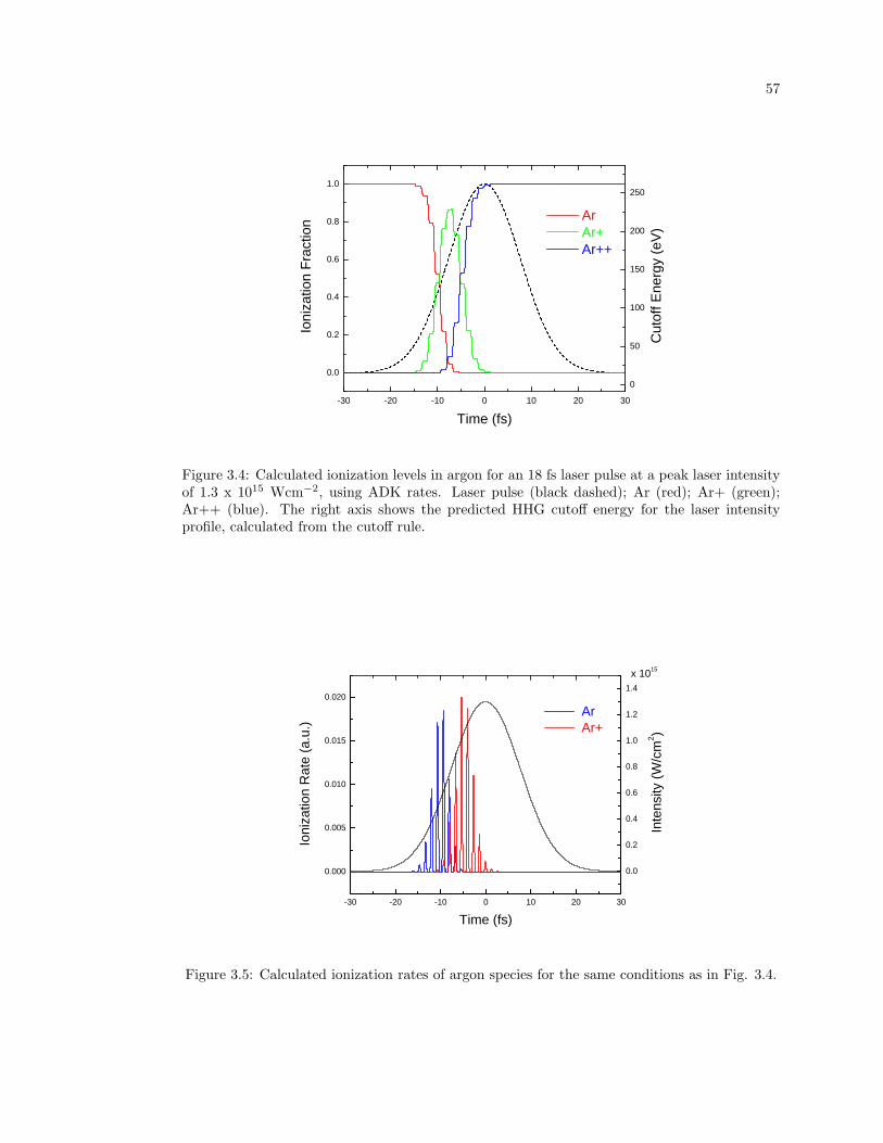
57

- 3 0 - 2 0 - 1 0 0 1 0 2 0 3 0

0 . 0

0 . 2

0 . 4

0 . 6

0 . 8

1 . 0

0

5 0

1 0 0

1 5 0

2 0 0

2 5 0

Ioniza

tion F

ractio

n

T i m e ( f s )

A r A r + A r + +

Cutof

f Ene

rgy (e

V)

Figure 3.4: Calculated ionization levels in argon for an 18 fs laser pulse at a peak laser intensityof 1.3 x 1015 Wcm−2, using ADK rates. Laser pulse (black dashed); Ar (red); Ar+ (green);Ar++ (blue). The right axis shows the predicted HHG cutoff energy for the laser intensityprofile, calculated from the cutoff rule.

- 3 0 - 2 0 - 1 0 0 1 0 2 0 3 0

0 . 0 0 0

0 . 0 0 5

0 . 0 1 0

0 . 0 1 5

0 . 0 2 0

0 . 0

0 . 2

0 . 4

0 . 6

0 . 8

1 . 0

1 . 2

1 . 4

Ioniza

tion R

ate (a

.u.)

T i m e ( f s )

A r A r +

x 1 0 1 5

Inten

sity (W

/cm2 )

Figure 3.5: Calculated ionization rates of argon species for the same conditions as in Fig. 3.4.

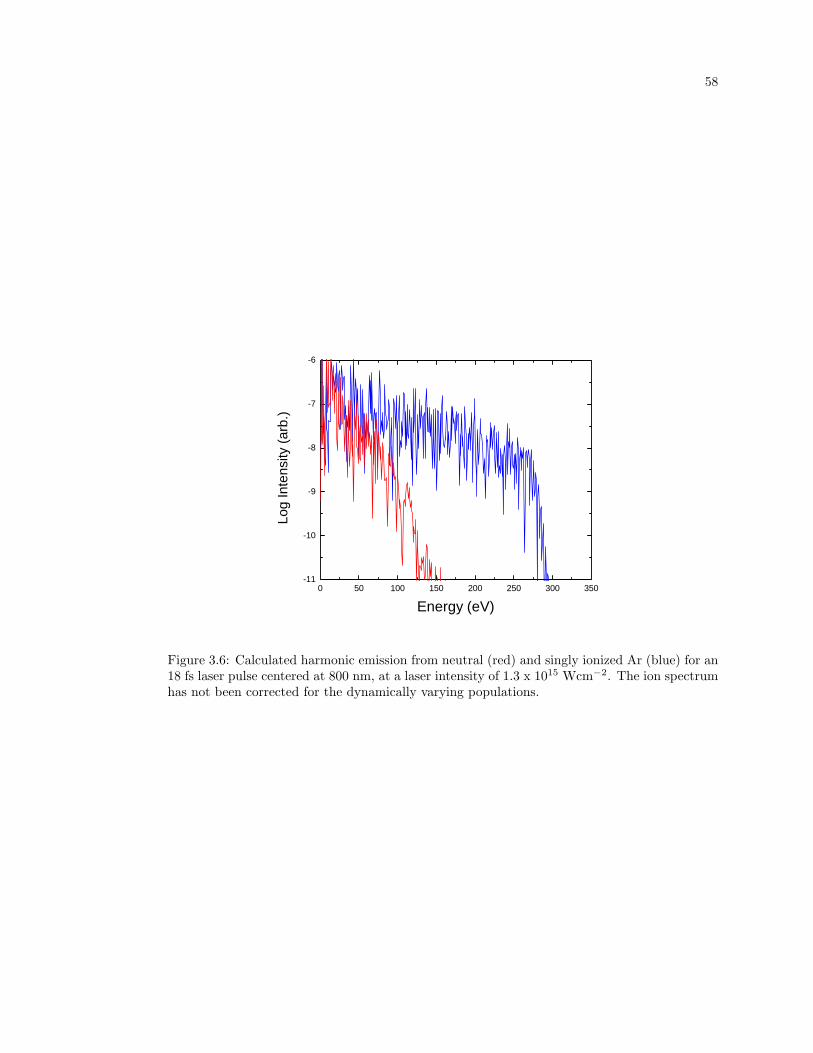
58

0 50 100 150 200 250 300 350-11

-10

-9

-8

-7

-6

Log I

ntens

ity (ar

b.)

Energy (eV)

Figure 3.6: Calculated harmonic emission from neutral (red) and singly ionized Ar (blue) for an18 fs laser pulse centered at 800 nm, at a laser intensity of 1.3 x 1015 Wcm−2. The ion spectrumhas not been corrected for the dynamically varying populations.

59

As further evidence for HHG from ions, we can compare the observed spectra with the

predictions of a fully quantum single-active electron approximation model that uses a soft core

potential to fit the ionization potential of the atom or ion under consideration.[37, 20] Only

qualitative comparisons are possible since the theory does not account for propagation effects or

the changing fraction of ionized species. Figure 3.6 shows predictions of the quantum model for

the harmonic spectrum emitted by Ar and Ar+ for an 18 fs driving-laser pulse at a peak intensity

of 1.3 x 1015 Wcm−2. The model predicts strong emission from neutrals up to photon energies

of 125 eV. For higher harmonics, the intensity drops rapidly by many orders of magnitude

with increasing harmonic order due to the complete ionization of Ar neutrals. In contrast,

emission from Ar+ is much stronger up to 260 eV. These theoretical predictions are in very

good qualitative agreement with our experimental observations. We also note that the quantum

calculations predict comparable emission intensities (i.e. effective nonlinear susceptibilities)

for neutrals and ions. This is consistent with our observations, which do not show a large

discontinuity in emission intensity with higher harmonic orders.

3.4 Validity of the ADK Model in the BSI Regime

One important question to address is whether the ADK model, which is valid in the

tunnelling ionization regime, is applicable in the barrier suppression ionization (BSI) regime.

Barrier suppression occurs when the electric field strength is comparable or greater than the

strength of the binding potential of the atom, allowing the electron to escape directly from the

potential well without tunnelling. This would lead to inaccuracies in the predictions of Figs.

3.4 and 3.5, although the quantum rate calculations and their predictions shown in Fig. 3.6 are

valid in this regime. Barrier suppression of an atom occurs for a field strength of Ebs = I2p/4, or,

in the case of Ar, an intensity of 2.5 x 1014 Wcm−2.[41, 5] Previous theoretical work has shown

that in this regime, ADK theory may overestimate the ionization rate and thus underestimate

the cutoff harmonic order from neutrals.[66, 71] Figure 3.7 shows the static field ionization rates

for H and He from a numerical solution of the time-dependent Schroedinger equation and from

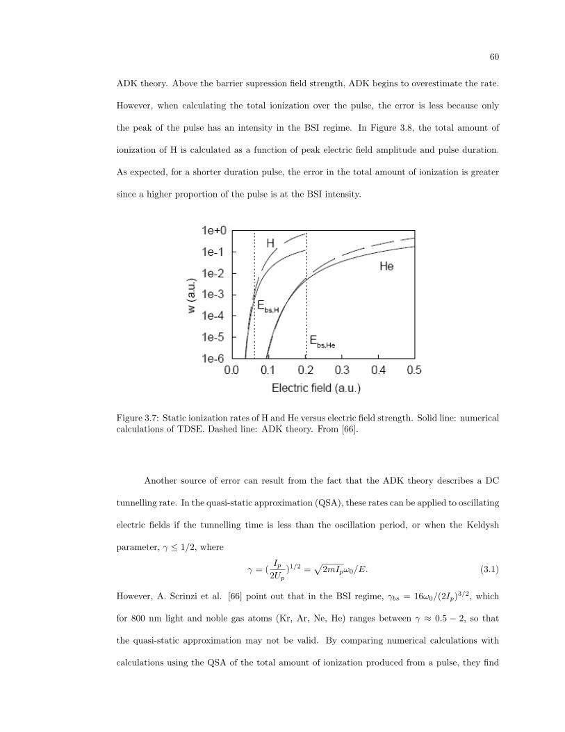
60

ADK theory. Above the barrier supression field strength, ADK begins to overestimate the rate.

However, when calculating the total ionization over the pulse, the error is less because only

the peak of the pulse has an intensity in the BSI regime. In Figure 3.8, the total amount of

ionization of H is calculated as a function of peak electric field amplitude and pulse duration.

As expected, for a shorter duration pulse, the error in the total amount of ionization is greater

since a higher proportion of the pulse is at the BSI intensity.

Figure 3.7: Static ionization rates of H and He versus electric field strength. Solid line: numericalcalculations of TDSE. Dashed line: ADK theory. From [66].

Another source of error can result from the fact that the ADK theory describes a DC

tunnelling rate. In the quasi-static approximation (QSA), these rates can be applied to oscillating

electric fields if the tunnelling time is less than the oscillation period, or when the Keldysh

parameter, γ ≤ 1/2, where

γ = (Ip

2Up)1/2 =

√2mIpω0/E. (3.1)

However, A. Scrinzi et al. [66] point out that in the BSI regime, γbs = 16ω0/(2Ip)3/2, which

for 800 nm light and noble gas atoms (Kr, Ar, Ne, He) ranges between γ ≈ 0.5 − 2, so that

the quasi-static approximation may not be valid. By comparing numerical calculations with

calculations using the QSA of the total amount of ionization produced from a pulse, they find

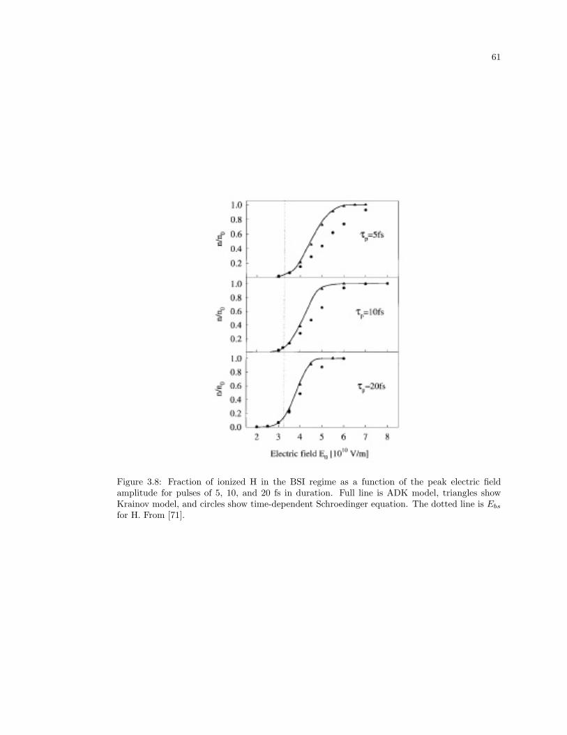
61

Figure 3.8: Fraction of ionized H in the BSI regime as a function of the peak electric fieldamplitude for pulses of 5, 10, and 20 fs in duration. Full line is ADK model, triangles showKrainov model, and circles show time-dependent Schroedinger equation. The dotted line is Ebs

for H. From [71].

62

that the deviation is less than 5% when the Keldysh parameter is between 0.5 < γ < 2 for 800

nm light. They conclude that the Keldysh condition which is calculated assuming tunnelling

ionization is not the same as for the BSI regime.

In our experiments, we use an 18 fs duration pulse with a peak intensity of 1.3 x 1015

Wcm−2. The peak electric field amplitude is Ep = 2.3Ebs for argon; however, the peak field

that the neutral argon atoms survive to will be somewhat less. From the calculations for He,

the actual rate is about 80% what ADK theory predicts when the field is twice the barrier

suppression field. Therefore the error in the ADK calculation of the total ionization fraction

during the pulse should not be significant. For Ar+, the calculated ionization rate using the

ADK model should be accurate, since we are below the barrier suppression intensity of the ion

(2.4 x 1015 Wcm−2) for our peak intensities. Previous work has shown very good agreement

between experiment and theory using ADK ionization rates for ions.[81, 17] Therefore, it is valid

to conclude that the significant extension of HHG we observe in Ar is due to emission from ions.

3.5 Plasma-induced Defocusing

We attribute our ability to observe these very high harmonic orders in argon primarily

to the use of a waveguide for high harmonic generation.[50] The waveguide minimizes the effect

of laser beam defocusing, resulting in high driving laser intensities even in the presence of

a substantial plasma. Theoretical calculations[59] and experimental observation[2] show that

plasma-induced defocusing effects limit the maximum intensity that can be achieved when a

laser is focused into an ionizing gas. These effects become significant when the defocusing

length, defined in Ref.[59] as lD = λnc/2ne, where ne is the electron density and nc is the

critical density, is smaller than the confocal parameter. In effect, the spatially varying plasma

creates a negative lens and the defocusing length is the length at which the phase advance at the

center of the beam is π/2. Under the conditions in our experiment, 100% ionized gas at 7 Torr,

the defocusing length is around 1 mm. This is an order of magnitude shorter than the laser

beam confocal parameter of ∼ 1 cm, and indicates that without the waveguide, the ionizing

63

gas would defocus the pulse before reaching its peak intensity. Experimentally, we observe that

the transverse profile of the beam emerging from a 2.5 cm long waveguide is unaffected by the

presence of the ionized gas for argon pressures up to 7 Torr, and that the energy decreases by

10-15%. This energy loss corresponds to a deposited energy of ∼30 eV for each atom in the

waveguide, and will lead to double-ionization of atoms in the center of the waveguide. We also

observe a significant spectral broadening, blueshifting of around 20-50 nm, and a shorter pulse

duration (from 22 fs to 18 fs) of the driving laser pulse when the gas is present, all of which

are indicative of a strong laser-plasma interaction that would be enhanced with guiding. At the

high laser intensities and ionization levels present in the waveguide, spectral broadening of the

harmonic peaks can also occur, as seen in Fig. 3.3.

When the argon pressure is increased above 9 Torr, the output mode breaks up and

harmonics are no longer observed. Therefore, there exists a limit to the amount of ionization-

induced defocusing for which the waveguide can compensate. Experimentally, we observe that

reducing the gas pressure in the waveguide will lead to an increase in the highest observed photon

energy. Figure 3.9 shows HHG spectra for argon at 5 and 7 Torr in a straight waveguide. At

the lower pressure, the flux at lower photon energies is reduced, but the higher photon energies

are enhanced. Figure 3.10 shows a more dramatic result for harmonics from neon at the same

intensity. There are several possible explanations for these results. It is possible that there is

still some defocusing effect which increases with higher pressures, reducing the intensity. Also, at

higher gas pressures, the laser energy at the output of the fiber is reduced, either from ionization

or from other loss mechanisms in the waveguide. The reduction in laser energy and therefore

intensity could also explain the decrease in harmonic energy.

The ability to generate harmonics in highly ionized media and from atomic ions holds

great promise to advance the energy range and flux of soft x-ray sources from HHG. Previously,

it was believed by many in the field that the limit to HHG energy was the saturation intensity.

In this work, we demonstrate that the true limit is given by the cutoff rule. In Chapter 2, it was

shown that the flux can be enhanced by using modulated waveguides even in 100 % ionization.

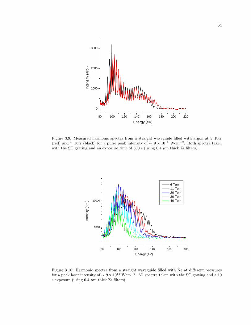
64

8 0 1 0 0 1 2 0 1 4 0 1 6 0 1 8 0 2 0 0 2 2 0

0

1 0 0 0

2 0 0 0

3 0 0 0

Inten

sity (a

rb.)

E n e r g y ( e V )

Figure 3.9: Measured harmonic spectra from a straight waveguide filled with argon at 5 Torr(red) and 7 Torr (black) for a pulse peak intensity of ∼ 9 x 1014 Wcm−2. Both spectra takenwith the SC grating and an exposure time of 300 s (using 0.4 µm thick Zr filters).

8 0 1 0 0 1 2 0 1 4 0 1 6 0 1 8 0

1 0 0 0

1 0 0 0 0

Inten

sity (a

rb.)

E n e r g y ( e V )

6 T o r r 1 1 T o r r 2 0 T o r r 3 0 T o r r 4 0 T o r r

Figure 3.10: Harmonic spectra from a straight waveguide filled with Ne at different pressuresfor a peak laser intensity of ∼ 9 x 1014 Wcm−2. All spectra taken with the SC grating and a 10s exposure (using 0.4 µm thick Zr filters).

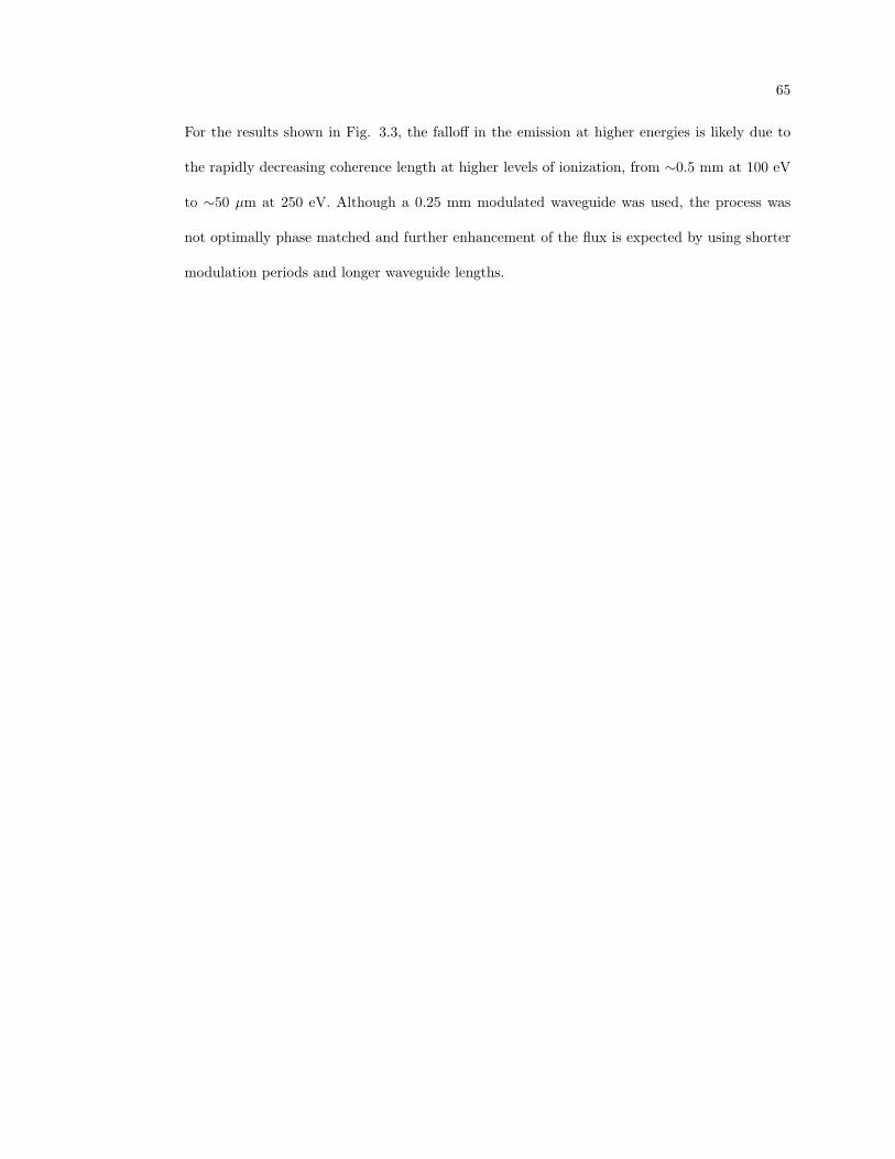
65

For the results shown in Fig. 3.3, the falloff in the emission at higher energies is likely due to

the rapidly decreasing coherence length at higher levels of ionization, from ∼0.5 mm at 100 eV

to ∼50 µm at 250 eV. Although a 0.25 mm modulated waveguide was used, the process was

not optimally phase matched and further enhancement of the flux is expected by using shorter

modulation periods and longer waveguide lengths.

Chapter 4

High Harmonic Generation Experimental Set-up

In this chapter, I discuss the experimental apparatus design and calibration used for the

results of Chapters 2 and 3. The laser system was designed by Sterling Backus and was originally

built by Sterling Backus and Randy Bartels. It is comprised of a 1 kHz two stage Ti:Sapphire

amplifier system, shown schematically in Figure 4.1.[8] The output of a Ti:Sapphire oscillator is

stretched to 200 ps using a grating stretcher, then passes through a zero length stretcher with

a deformable mirror in the focal plane where the pulse is spectrally dispersed. The low energy

pulse is then amplified in two stages to a final output pulse energy of 5 mJ, using 2 pump lasers

on the 2nd stage. The amplified output is compressed in time with a grating compressor. The

deformable mirror is used in conjunction with an Evolutionary Strategy algorithm to optimize

the second harmonic signal, giving a final compressed pulse width of ∼22 fs +/- 2 fs. The loss

from the grating compressor reduces the compressed signal to around 3 mJ.

The laser is focused with a 50 cm focal length mirror into a 150 µm inner-diameter

hollow-core waveguide with a coupling efficiency of ∼ 60%.

Figure 4.2 shows the experimental setup for high harmonic generation. The laser is

focused through a 250 µm-thick sapphire window and into the waveguide setup. The central,

2.5 cm fiber is held in a glass capillary with holes drilled in it to allow input of the gas, and there

are two small fiber sections at each end which allow differential pumping to vacuum on either

side. The harmonic signal and residual fundamental 800 nm light exit the waveguide into the rest

of the vacuum chamber. A valve after the waveguide setup makes it possible to vent and change

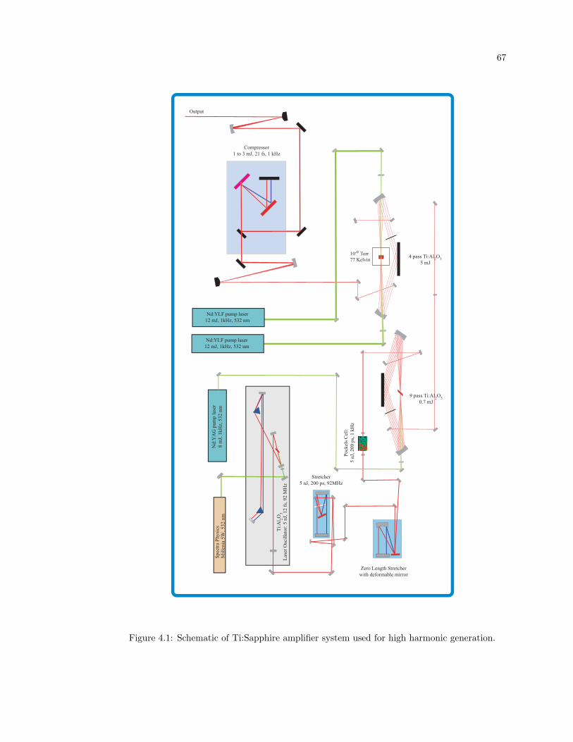
67

10 Torr77 Kelvin

-9

Figure 4.1: Schematic of Ti:Sapphire amplifier system used for high harmonic generation.

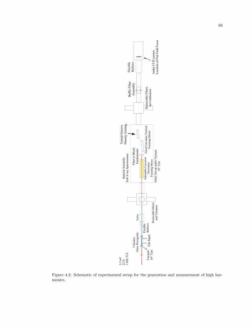
68

3 Se

ctio

n G

lass

Wav

egui

de

Gas

Inpu

t

Val

ve

Vac

uum

10

To

rr-3

Rem

ovab

le M

irror

and

Vie

wpo

rt

Rem

ovab

le F

ilter

sfo

r Cal

ibra

tion

Filte

r to

Blo

ckFu

ndam

enta

l

Entir

e Se

t-up

unde

r Vac

uum

10

Torr

-6

Baf

fle F

ilter

Ass

embl

y

And

or C

CD

cam

era

Loca

tion

of F

lat F

ield

Foc

us

Adj

usta

ble

Cur

vatu

re

Hor

izon

tal

Focu

sing

Mirr

or

Fixe

d C

urva

ture

Ver

tical

Focu

sing

Mirr

or

Var

ied-

Gro

ove

Den

sity

Gra

ting

Het

trick

Sci

entif

ic

Soft

X-r

ay S

pect

rom

eter

Flex

ible

B

ello

ws

Flex

ible

B

ello

ws

1-3

mJ

22 fs

1 kH

z Ti

:S

Figure 4.2: Schematic of experimental setup for the generation and measurement of high har-monics.

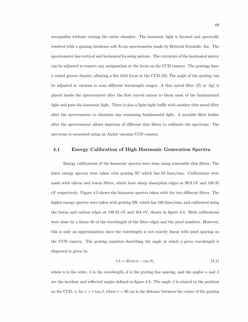
69

waveguides without venting the entire chamber. The harmonic light is focused and spectrally

resolved with a grazing incidence soft X-ray spectrometer made by Hettrick Scientific, Inc. The

spectrometer has vertical and horizontal focusing mirrors. The curvature of the horizontal mirror

can be adjusted to remove any astigmatism at the focus on the CCD camera. The gratings have

a varied groove density, allowing a flat field focus at the CCD.[35] The angle of the grating can

be adjusted in vacuum to scan different wavelength ranges. A thin metal filter (Zr or Ag) is

placed inside the spectrometer after the first curved mirror to block most of the fundamental

light and pass the harmonic light. There is also a light-tight baffle with another thin metal filter

after the spectrometer to eliminate any remaining fundamental light. A movable filter holder

after the spectrometer allows insertion of different thin filters to calibrate the spectrum. The

spectrum is measured using an Andor vacuum CCD camera.

4.1 Energy Calibration of High Harmonic Generation Spectra

Energy calibrations of the harmonic spectra were done using removable thin filters. The

lower energy spectra were taken with grating SC which has 65 lines/mm. Calibrations were

made with silicon and boron filters, which have sharp absorption edges at 99.9 eV and 188.35

eV respectively. Figure 4.3 shows the harmonic spectra taken with the two different filters. The

higher energy spectra were taken with grating SB, which has 160 lines/mm, and calibrated using

the boron and carbon edges at 188.35 eV and 284 eV, shown in figure 4.4. Both calibrations

were done by a linear fit of the wavelength of the filter edges and the pixel numbers. However,

this is only an approximation since the wavelength is not exactly linear with pixel spacing on

the CCD camera. The grating equation describing the angle at which a given wavelength is

dispersed is given by,

nλ = d(cos α− cos β), (4.1)

where n is the order, λ is the wavelength, d is the grating line spacing, and the angles α and β

are the incident and reflected angles defined in figure 4.5. The angle β is related to the position

on the CCD, x, by x = r tanβ, where r ∼ 80 cm is the distance between the center of the grating

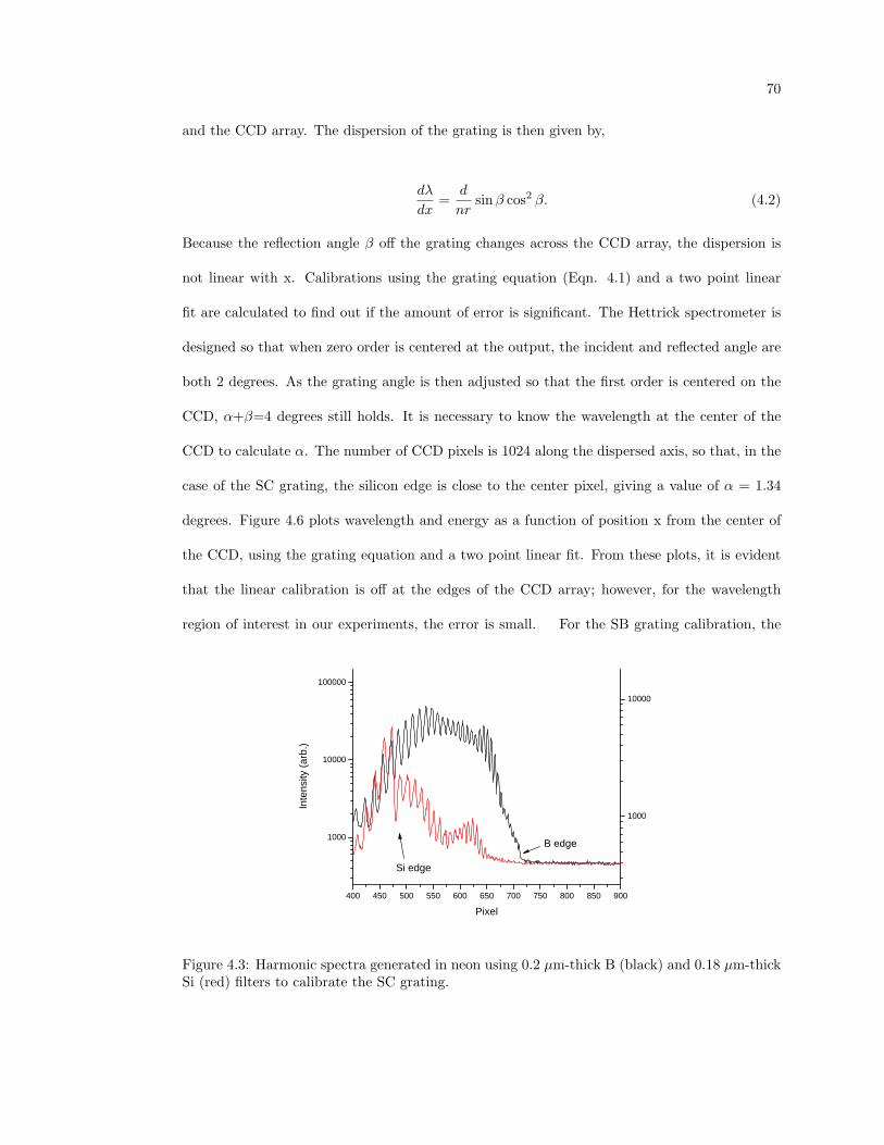
70

and the CCD array. The dispersion of the grating is then given by,

dλ

dx=

d

nrsinβ cos2 β. (4.2)

Because the reflection angle β off the grating changes across the CCD array, the dispersion is

not linear with x. Calibrations using the grating equation (Eqn. 4.1) and a two point linear

fit are calculated to find out if the amount of error is significant. The Hettrick spectrometer is

designed so that when zero order is centered at the output, the incident and reflected angle are

both 2 degrees. As the grating angle is then adjusted so that the first order is centered on the

CCD, α+β=4 degrees still holds. It is necessary to know the wavelength at the center of the

CCD to calculate α. The number of CCD pixels is 1024 along the dispersed axis, so that, in the

case of the SC grating, the silicon edge is close to the center pixel, giving a value of α = 1.34

degrees. Figure 4.6 plots wavelength and energy as a function of position x from the center of

the CCD, using the grating equation and a two point linear fit. From these plots, it is evident

that the linear calibration is off at the edges of the CCD array; however, for the wavelength

region of interest in our experiments, the error is small. For the SB grating calibration, the

4 0 0 4 5 0 5 0 0 5 5 0 6 0 0 6 5 0 7 0 0 7 5 0 8 0 0 8 5 0 9 0 0

1 0 0 0

1 0 0 0 0

1 0 0 0 0 0

1 0 0 0

1 0 0 0 0

Inten

sity (a

rb.)

P i x e l

B e d g eS i e d g e

Figure 4.3: Harmonic spectra generated in neon using 0.2 µm-thick B (black) and 0.18 µm-thickSi (red) filters to calibrate the SC grating.

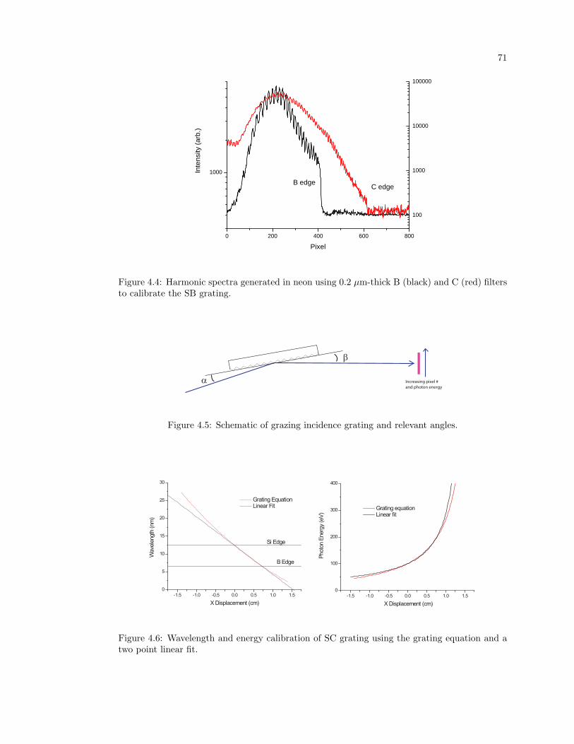
71

0 2 0 0 4 0 0 6 0 0 8 0 0

1 0 0 0

1 0 0

1 0 0 0

1 0 0 0 0

1 0 0 0 0 0

C e d g eInt

ensity

(arb.

)

P i x e l

B e d g e

Figure 4.4: Harmonic spectra generated in neon using 0.2 µm-thick B (black) and C (red) filtersto calibrate the SB grating.

α

β

Increasing pixel #and photon energy

Figure 4.5: Schematic of grazing incidence grating and relevant angles.

-1.5 -1.0 -0.5 0.0 0.5 1.0 1.50

5

10

15

20

25

30

B Edge

Wav

elen

gth

(nm

)

X Displacement (cm)

Grating Equation Linear Fit

Si Edge

-1.5 -1.0 -0.5 0.0 0.5 1.0 1.50

100

200

300

400

X Displacement (cm)

Phot

on E

nerg

y (e

V)

Grating equation Linear fit

Figure 4.6: Wavelength and energy calibration of SC grating using the grating equation and atwo point linear fit.

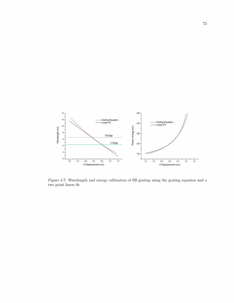
72

-1.5 -1.0 -0.5 0.0 0.5 1.0 1.5

100

200

300

400

500

Phot

on E

nerg

y (e

V)

X Displacement (cm)

Grating Equation Linear Fit

-1.5 -1.0 -0.5 0.0 0.5 1.0 1.50

2

4

6

8

10

12

14

C EdgeWav

elen

gth

(nm

)

X Displacement (cm)

Grating Equation Linear Fit

B Edge

Figure 4.7: Wavelength and energy calibration of SB grating using the grating equation and atwo point linear fit.

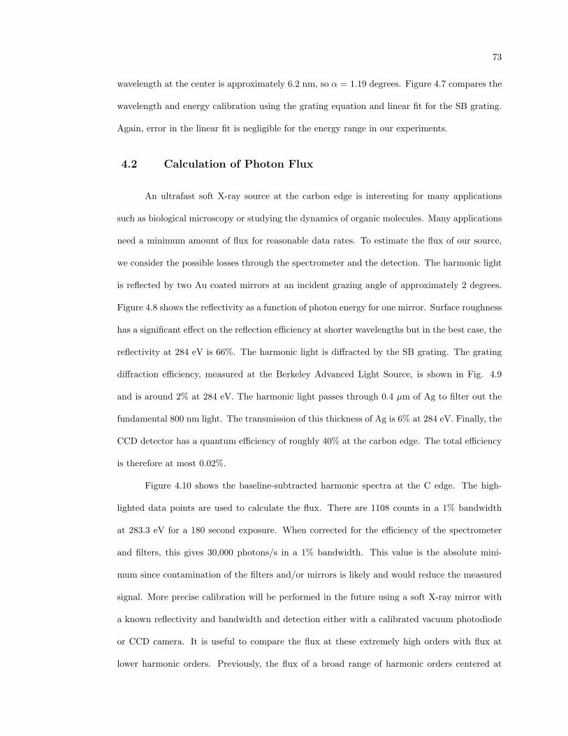
73

wavelength at the center is approximately 6.2 nm, so α = 1.19 degrees. Figure 4.7 compares the

wavelength and energy calibration using the grating equation and linear fit for the SB grating.

Again, error in the linear fit is negligible for the energy range in our experiments.

4.2 Calculation of Photon Flux

An ultrafast soft X-ray source at the carbon edge is interesting for many applications

such as biological microscopy or studying the dynamics of organic molecules. Many applications

need a minimum amount of flux for reasonable data rates. To estimate the flux of our source,

we consider the possible losses through the spectrometer and the detection. The harmonic light

is reflected by two Au coated mirrors at an incident grazing angle of approximately 2 degrees.

Figure 4.8 shows the reflectivity as a function of photon energy for one mirror. Surface roughness

has a significant effect on the reflection efficiency at shorter wavelengths but in the best case, the

reflectivity at 284 eV is 66%. The harmonic light is diffracted by the SB grating. The grating

diffraction efficiency, measured at the Berkeley Advanced Light Source, is shown in Fig. 4.9

and is around 2% at 284 eV. The harmonic light passes through 0.4 µm of Ag to filter out the

fundamental 800 nm light. The transmission of this thickness of Ag is 6% at 284 eV. Finally, the

CCD detector has a quantum efficiency of roughly 40% at the carbon edge. The total efficiency

is therefore at most 0.02%.

Figure 4.10 shows the baseline-subtracted harmonic spectra at the C edge. The high-

lighted data points are used to calculate the flux. There are 1108 counts in a 1% bandwidth

at 283.3 eV for a 180 second exposure. When corrected for the efficiency of the spectrometer

and filters, this gives 30,000 photons/s in a 1% bandwidth. This value is the absolute mini-

mum since contamination of the filters and/or mirrors is likely and would reduce the measured

signal. More precise calibration will be performed in the future using a soft X-ray mirror with

a known reflectivity and bandwidth and detection either with a calibrated vacuum photodiode

or CCD camera. It is useful to compare the flux at these extremely high orders with flux at

lower harmonic orders. Previously, the flux of a broad range of harmonic orders centered at

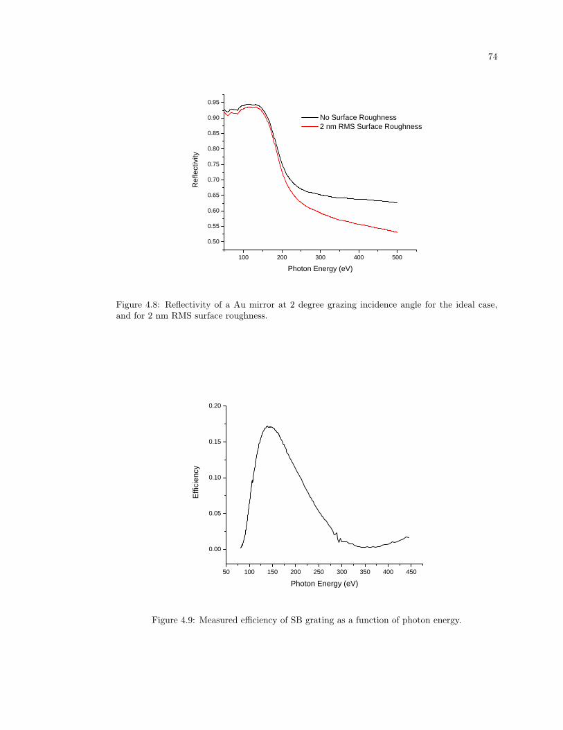
74

1 0 0 2 0 0 3 0 0 4 0 0 5 0 0

0 . 5 00 . 5 50 . 6 00 . 6 50 . 7 00 . 7 50 . 8 00 . 8 50 . 9 00 . 9 5

Refle

ctivity

P h o t o n E n e r g y ( e V )

N o S u r f a c e R o u g h n e s s 2 n m R M S S u r f a c e R o u g h n e s s

Figure 4.8: Reflectivity of a Au mirror at 2 degree grazing incidence angle for the ideal case,and for 2 nm RMS surface roughness.

5 0 1 0 0 1 5 0 2 0 0 2 5 0 3 0 0 3 5 0 4 0 0 4 5 0

0 . 0 0

0 . 0 5

0 . 1 0

0 . 1 5

0 . 2 0

Efficie

ncy

P h o t o n E n e r g y ( e V )

Figure 4.9: Measured efficiency of SB grating as a function of photon energy.

75

31 eV (harmonic orders 17-23) was measured using a vacuum photodiode.[10] The harmonics

were generated with a 5 kHz repetition rate laser in argon using a 10 cm long hollow-core 150

µm inner-diameter waveguide. The measured flux was ∼ 2 x 1012 photons/second. For further

comparison, Fig. 4.11 shows the flux from the soft X-ray beamline at the Advanced Light Source

at Berkeley. At the carbon edge, an estimated flux of 1013 photons/s in a 0.1% bandwidth is

produced before the monochromator. Despite the higher photon flux of the Advanced Light

Source, the pulse duration much greater than that of the soft x-ray light produced from HHG.

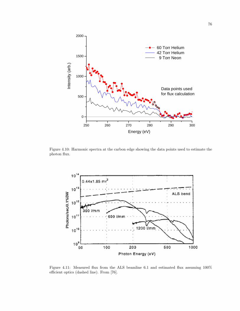
76

2 5 0 2 6 0 2 7 0 2 8 0 2 9 0 3 0 00

5 0 0

1 0 0 0

1 5 0 0

2 0 0 0

Inten

sity (a

rb.)

E n e r g y ( e V )

6 0 T o r r H e l i u m 4 2 T o r r H e l i u m 9 T o r r N e o n

D a t a p o i n t s u s e df o r f l u x c a l c u l a t i o n

Figure 4.10: Harmonic spectra at the carbon edge showing the data points used to estimate thephoton flux.

Figure 4.11: Measured flux from the ALS beamline 6.1 and estimated flux assuming 100%efficient optics (dashed line). From [76].

Chapter 5

Self-compression of Intense Femtosecond Pulses in Gas-filled

Hollow-core Waveguides

One surprising experimental result that came out of my research on high harmonic gener-

ation was the observation of temporal compression of the 800 nm driving pulse after propagating

in a hollow-core waveguide filled with low-pressure argon at ionizing intensities. Unlike other

standard pulse compression techniques, no subsequent dispersion compensation was used. Typ-

ically, pulse compression is accomplished by broadening of the spectrum of the pulse through

nonlinear self-phase modulation. This broadened pulse bandwidth can then be compressed to a

shorter pulse by appropriate dispersion compensation. Self-phase modulation of the pulse can

be done by propagation through an optical fiber[53, 73] or a gas-filled hollow waveguide[54] at

non-ionizing intensities and dispersion compensation is provided by prisms, gratings, or chirped

mirrors to create a negative group velocity dispersion. These schemes have been employed to

compress pulses to under 4 fs pulse duration[82]; however, such techniques are lossy and can be

quite complicated. Furthermore, all previous pulse compression schemes have been limited to

sub-millijoule pulse energies due to the damage threshold of the fibers or ionization of the gas.

The use of ionization to broaden the spectrum of a pulse for compression has been previously

considered theoretically.[72] However, the compression also depended on negative group velocity

dispersion compensation.

78

5.1 Experimental Results

In the experiment, light from a Ti:sapphire amplifier producing ∼ 30 fs near-transform

limited pulses with 2.5 mJ pulse energies at 1 kHz was focused into a 2.5 cm long, 150 micron

inner-diameter hollow waveguide filled with low pressure argon. The spot diameter of the laser

mode at the entrance of the waveguide was ∼ 85 µm FWHM and the energy throughput of

the waveguide was ∼ 60% with no gas. The focusing region before and after the waveguide

was held under vacuum to prevent any additional nonlinear effects. The pulse was charac-

terized before and after the waveguide using second-harmonic frequency-resolved-optical-gating

(SHG-FROG).[74] All FROG measurements were deconvolved using commercial software from

Femtosoft Technologies (FROG Version 3.03) to an error of < 1% for a 256x256 sampling grid.

The spectral marginals for each measurement agree with the experimentally measured spectra

to within 5%. After exiting the waveguide, the pulse passes through a 250 µm thick sapphire

window and a 1 mm thick fused silica beam splitter in the FROG setup. The total dispersion of

these elements corresponds to a group velocity dispersion of 61 fs2 and a third-order dispersion

of 40 fs3 at a center wavelength of 760 nm, which would change the pulse duration at most by 3

fs, not enough to significantly affect the experimental results. Also, the material gives a positive

group velocity dispersion, which would not explain pulse compression by the typical schemes.

The pulse shape after the fiber without gas is the same as the input to within our measurement

resolution.

The intensity in the waveguide, approximately 1015 W/cm2, is high enough to completely

doubly ionize the argon gas by the peak of the pulse (for a 30 fs duration pulse). This rapidly

changing ionization during the pulse results in an index of refraction that decreases with time,

causing a blue shift of the overall laser spectrum. The spectra at the exit of the waveguide with

varying pressures of argon is shown in figure 5.1. Pressures as low as 1 Torr result in significant

blue shift and spectral broadening and blue shifts of up to ∼ 50 nm are observed. Figure 5.2

shows the deconvolved FROG measurements of the temporal pulse shape after the waveguide

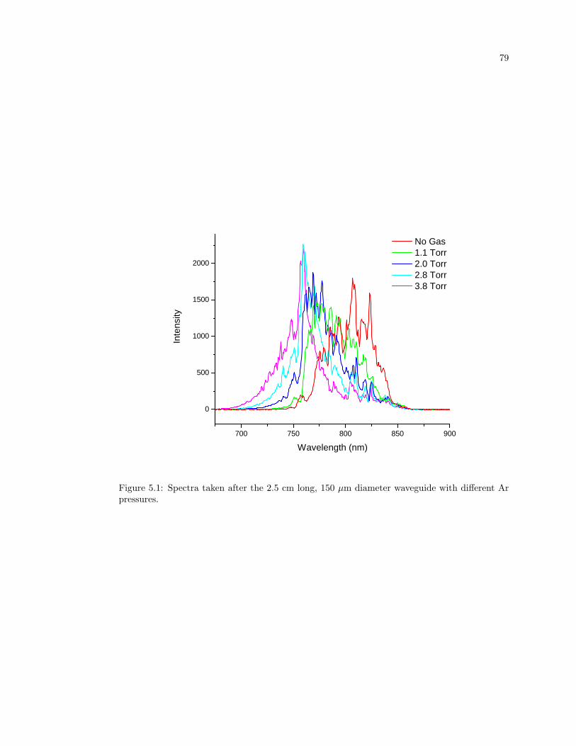
79

7 0 0 7 5 0 8 0 0 8 5 0 9 0 0

0

5 0 0

1 0 0 0

1 5 0 0

2 0 0 0

Inten

sity

W a v e l e n g t h ( n m )

N o G a s 1 . 1 T o r r 2 . 0 T o r r 2 . 8 T o r r 3 . 8 T o r r

Figure 5.1: Spectra taken after the 2.5 cm long, 150 µm diameter waveguide with different Arpressures.

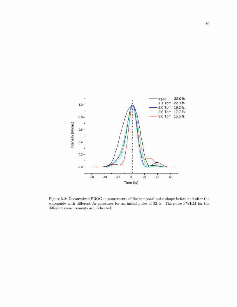
80

- 6 0 - 4 0 - 2 0 0 2 0 4 0 6 0

0 . 0

0 . 2

0 . 4

0 . 6

0 . 8

1 . 0

Inten

sity (N

orm.)

T i m e ( f s )

I n p u t 3 2 . 0 f s 1 . 1 T o r r 2 2 . 3 f s 2 . 0 T o r r 1 9 . 2 f s 2 . 8 T o r r 1 7 . 7 f s 3 . 8 T o r r 1 5 . 5 f s

Figure 5.2: Deconvolved FROG measurements of the temporal pulse shape before and after thewaveguide with different Ar pressures for an initial pulse of 32 fs. The pulse FWHM for thedifferent measurements are indicated.

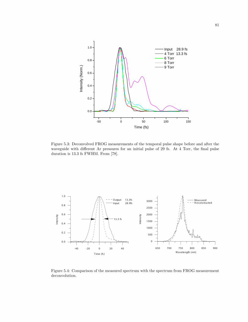
81

- 5 0 0 5 0 1 0 0 1 5 0

0 . 0

0 . 2

0 . 4

0 . 6

0 . 8

1 . 0

Inten

sity (N

orm.)

T i m e ( f s )

I n p u t 2 8 . 9 f s 4 T o r r 1 3 . 3 f s 6 T o r r 8 T o r r 9 T o r r

Figure 5.3: Deconvolved FROG measurements of the temporal pulse shape before and after thewaveguide with different Ar pressures for an initial pulse of 29 fs. At 4 Torr, the final pulseduration is 13.3 fs FWHM. From [78].

650 700 750 800 850 900

0

500

1000

1500

2000

2500

3000 Measured

Wavelength (nm)

Inte

nsi

ty

R econstructed

-40 -20 0 20 40

0.0

0.2

0.4

0.6

0.8

1.0

Inte

nsi

ty

T ime (fs )

Output 13.3fs Input 28.9fs

13.3 fs

Figure 5.4: Comparison of the measured spectrum with the spectrum from FROG measurementdeconvolution.

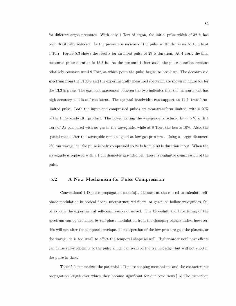
82

for different argon pressures. With only 1 Torr of argon, the initial pulse width of 32 fs has

been drastically reduced. As the pressure is increased, the pulse width decreases to 15.5 fs at

4 Torr. Figure 5.3 shows the results for an input pulse of 29 fs duration. At 4 Torr, the final

measured pulse duration is 13.3 fs. As the pressure is increased, the pulse duration remains

relatively constant until 9 Torr, at which point the pulse begins to break up. The deconvolved

spectrum from the FROG and the experimentally measured spectrum are shown in figure 5.4 for

the 13.3 fs pulse. The excellent agreement between the two indicates that the measurement has

high accuracy and is self-consistent. The spectral bandwidth can support an 11 fs transform-

limited pulse. Both the input and compressed pulses are near-transform limited, within 20%

of the time-bandwidth product. The power exiting the waveguide is reduced by ∼ 5 % with 4

Torr of Ar compared with no gas in the waveguide, while at 8 Torr, the loss is 10%. Also, the

spatial mode after the waveguide remains good at low gas pressures. Using a larger diameter,

230 µm waveguide, the pulse is only compressed to 24 fs from a 30 fs duration input. When the

waveguide is replaced with a 1 cm diameter gas-filled cell, there is negligible compression of the

pulse.

5.2 A New Mechanism for Pulse Compression

Conventional 1-D pulse propagation models[1, 13] such as those used to calculate self-

phase modulation in optical fibers, microstructured fibers, or gas-filled hollow waveguides, fail

to explain the experimental self-compression observed. The blue-shift and broadening of the

spectrum can be explained by self-phase modulation from the changing plasma index; however,

this will not alter the temporal envelope. The dispersion of the low-pressure gas, the plasma, or

the waveguide is too small to affect the temporal shape as well. Higher-order nonlinear effects

can cause self-steepening of the pulse which can reshape the trailing edge, but will not shorten

the pulse in time.

Table 5.2 summarizes the potential 1-D pulse shaping mechanisms and the characteristic

propagation length over which they become significant for our conditions.[13] The dispersion

83

length is given by:

Ldis =T 2

| d2kdω2 |,

(5.1)

where T is the pulse duration (1/e intensity) and k = ωn/c. For a 30 fs pulse FWHM, T =

18 fs. The dispersion length is the length over which the pulse duration would approximately

double due to group velocity dispersion (GVD). Self-phase modulation becomes important when

the spectral broadening is on the order of the spectral width of the initial pulse. The amount of

SPM broadening is given approximately by dφ(ω)/dt or ∼ ∆φNL/T where ∆φNL ∼ n2IωL/c.

The bandwidth of the input pulse is approximately 1/T . Therefore, SPM is significant when

∆φNL ∼ 1 and the effective length is given by:

LSPM =c

ωn2I. (5.2)

Another nonlinear mechanism is self-steepening of the pulse. The self-steepening process

depends on the nonlinear group index which is defined as n(g)2 = n2 + ω dn2

dω . In our case, the

assumption n(g)2 ≈ n2 is valid. The effective length over which self steepening is significant is

given by:

LSS =cT

n(g)2 I

. (5.3)

Lastly, the time-varying index due to ionization during the pulse also affects the pulse

spectrum. The plasma index is given by:

np =

√1−

ω2p

ω2' 1−

ω2p

2ω2,(5.4)

where ωp is the plasma frequency given by: ω2p = Nee

2/mε0, e and m are the electron charge and

mass, and Ne is the electron density. Because the electron density is increasing in time during

the leading part of the pulse, the plasma index is also changing during the pulse. In this way, the

plasma index acts like the nonlinear index, n2I, the difference being that it only decreases during

the pulse, instead of increasing and decreasing over the duration of the pulse. Therefore, the

spectrum predominately broadens to shorter wavelengths. The length over which the effective

nonlinear index from the plasma will affect the spectrum from self-phase modulation is given by

LPlasmaSPM = c/ωnp and the effective self-steepening length given by LPlasmaSS = cT/np.

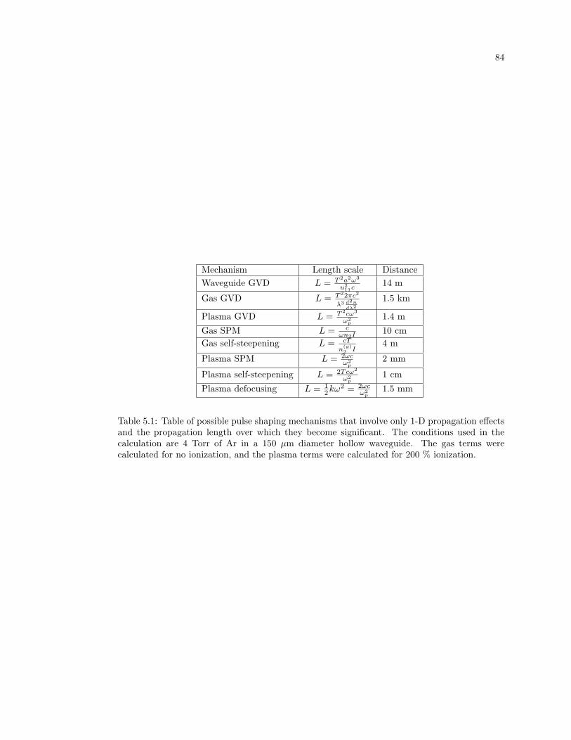
84

Mechanism Length scale DistanceWaveguide GVD L = T 2a2ω3

u211c

14 m

Gas GVD L = T 22πc2

λ3 d2ndλ2

1.5 km

Plasma GVD L = T 2cω3

ω2p

1.4 mGas SPM L = c

ωn2I 10 cmGas self-steepening L = cT

n(g)2 I

4 m

Plasma SPM L = 2ωcω2

p2 mm

Plasma self-steepening L = 2Tcω2

ω2p

1 cm

Plasma defocusing L = 12kω2 = 2ωc

ω2p

1.5 mm

Table 5.1: Table of possible pulse shaping mechanisms that involve only 1-D propagation effectsand the propagation length over which they become significant. The conditions used in thecalculation are 4 Torr of Ar in a 150 µm diameter hollow waveguide. The gas terms werecalculated for no ionization, and the plasma terms were calculated for 200 % ionization.

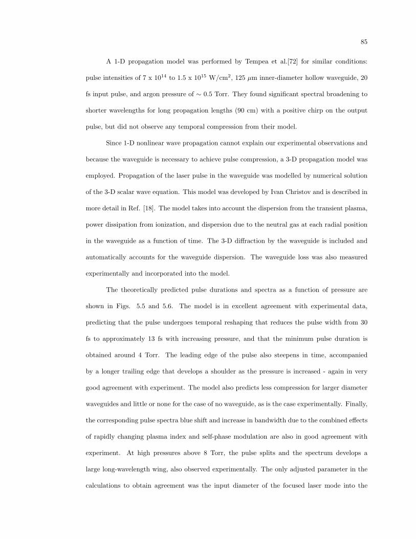
85

A 1-D propagation model was performed by Tempea et al.[72] for similar conditions:

pulse intensities of 7 x 1014 to 1.5 x 1015 W/cm2, 125 µm inner-diameter hollow waveguide, 20

fs input pulse, and argon pressure of ∼ 0.5 Torr. They found significant spectral broadening to

shorter wavelengths for long propagation lengths (90 cm) with a positive chirp on the output

pulse, but did not observe any temporal compression from their model.

Since 1-D nonlinear wave propagation cannot explain our experimental observations and

because the waveguide is necessary to achieve pulse compression, a 3-D propagation model was

employed. Propagation of the laser pulse in the waveguide was modelled by numerical solution

of the 3-D scalar wave equation. This model was developed by Ivan Christov and is described in

more detail in Ref. [18]. The model takes into account the dispersion from the transient plasma,

power dissipation from ionization, and dispersion due to the neutral gas at each radial position

in the waveguide as a function of time. The 3-D diffraction by the waveguide is included and

automatically accounts for the waveguide dispersion. The waveguide loss was also measured

experimentally and incorporated into the model.

The theoretically predicted pulse durations and spectra as a function of pressure are

shown in Figs. 5.5 and 5.6. The model is in excellent agreement with experimental data,

predicting that the pulse undergoes temporal reshaping that reduces the pulse width from 30

fs to approximately 13 fs with increasing pressure, and that the minimum pulse duration is

obtained around 4 Torr. The leading edge of the pulse also steepens in time, accompanied

by a longer trailing edge that develops a shoulder as the pressure is increased - again in very

good agreement with experiment. The model also predicts less compression for larger diameter

waveguides and little or none for the case of no waveguide, as is the case experimentally. Finally,

the corresponding pulse spectra blue shift and increase in bandwidth due to the combined effects

of rapidly changing plasma index and self-phase modulation are also in good agreement with

experiment. At high pressures above 8 Torr, the pulse splits and the spectrum develops a

large long-wavelength wing, also observed experimentally. The only adjusted parameter in the

calculations to obtain agreement was the input diameter of the focused laser mode into the

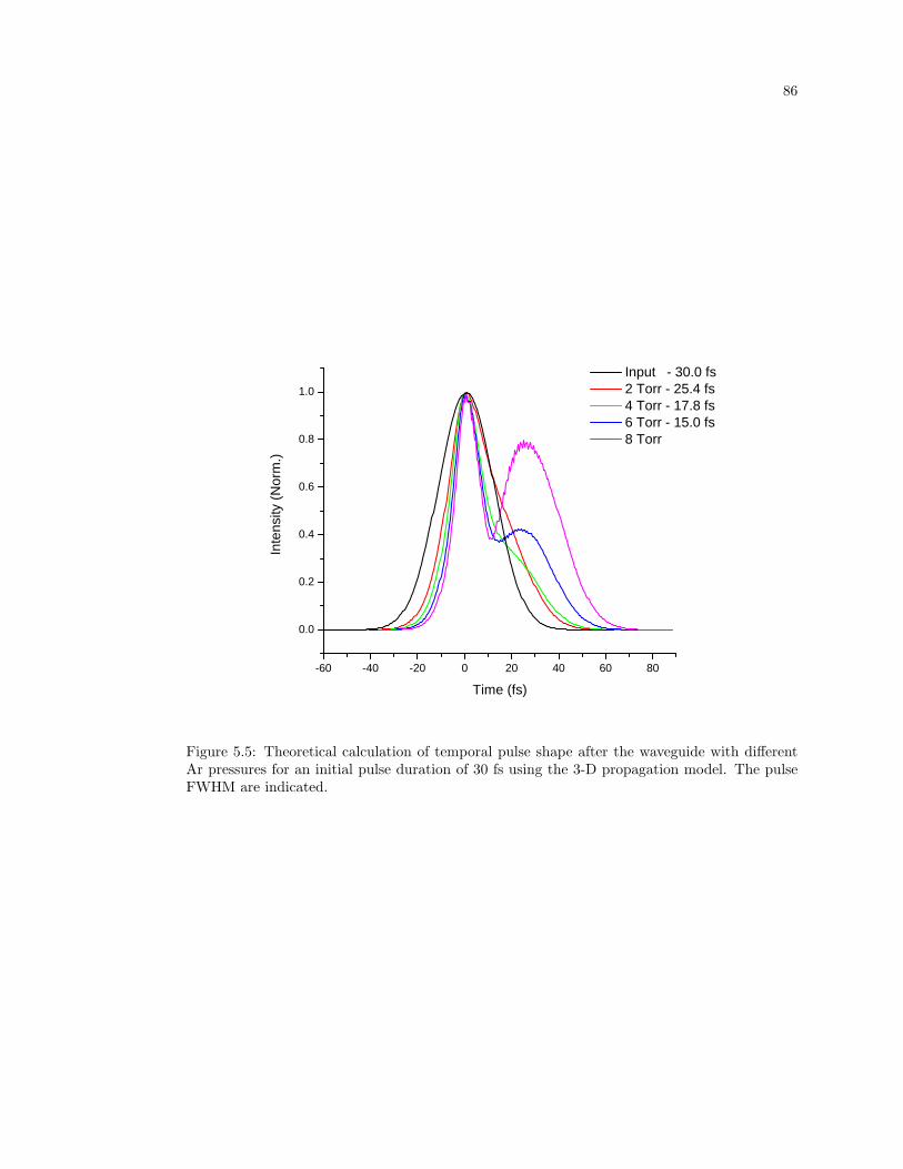
86

- 6 0 - 4 0 - 2 0 0 2 0 4 0 6 0 8 0

0 . 0

0 . 2

0 . 4

0 . 6

0 . 8

1 . 0 I n p u t - 3 0 . 0 f s 2 T o r r - 2 5 . 4 f s 4 T o r r - 1 7 . 8 f s 6 T o r r - 1 5 . 0 f s 8 T o r r

Inten

sity (N

orm.)

T i m e ( f s )

Figure 5.5: Theoretical calculation of temporal pulse shape after the waveguide with differentAr pressures for an initial pulse duration of 30 fs using the 3-D propagation model. The pulseFWHM are indicated.

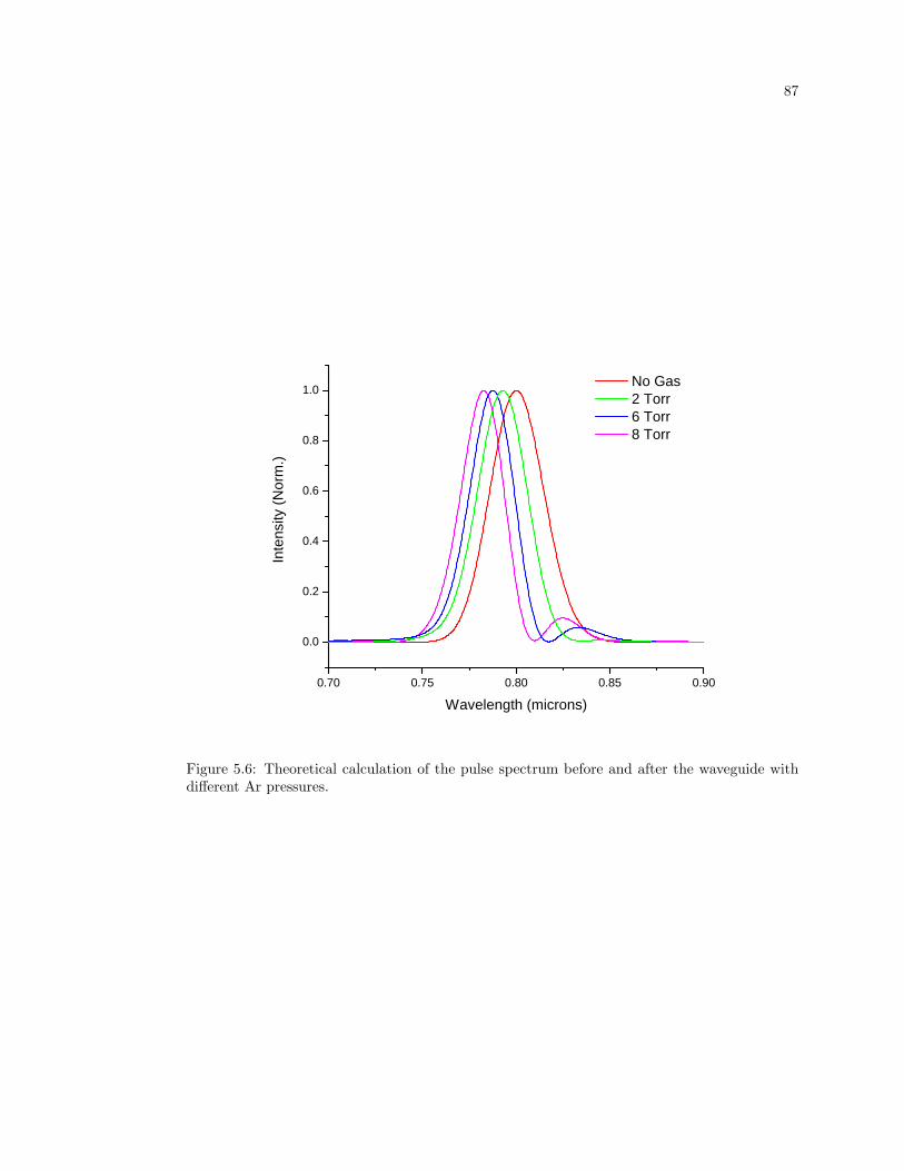
87

0 . 7 0 0 . 7 5 0 . 8 0 0 . 8 5 0 . 9 0

0 . 0

0 . 2

0 . 4

0 . 6

0 . 8

1 . 0

Inten

sity (N

orm.)

W a v e l e n g t h ( m i c r o n s )

N o G a s 2 T o r r 6 T o r r 8 T o r r

Figure 5.6: Theoretical calculation of the pulse spectrum before and after the waveguide withdifferent Ar pressures.

88

waveguide.

The self-compression is a result of the combined effects of plasma-induced refraction and

blue shifting, diffraction of the laser beam, phase modulation due to the rapidly-changing plasma

index, and guiding by the hollow waveguide. The role of plasma defocusing combined with the

waveguide refocusing governs the spatial propagation and is very important in the compression

process. The model shows that as the pulse begins to ionize the gas, the trailing edge of the

pulse refracts from the center of the waveguide due to plasma-induced defocusing. However,

this portion of the beam is then reflected back into the guide by the waveguide walls. This

leads to a temporally compressed pulse with a sharp leading edge and flat temporal phase. The

reshaping also leads to a small periodic oscillation in the beam diameter and pulsewidth as the

pulse propagates down the waveguide. This high-field pulse reshaping process has similarities

with passive mode locking of lasers using saturable absorbers - the trailing edge of the pulse is

slowly depleted periodically along the waveguide due to ionization-induced defocusing, where

the role of a laser resonator is replaced by the waveguide. Both experimentally and theoretically,

the pulse compression process is sensitive to the initial mode coupled into the waveguide. Also,

theoretically, the laser beam must be focused to a tighter focal spot diameter than the ideal

100 µm for coupling into the lowest-order mode of 150 µm waveguide, in agreement with our

experimental observations.

A new mechanism for pulse compression that operates at laser intensities above the ion-

ization threshold has been demonstrated both theoretically and experimentally. This technique

allows compression of pulses with millijoule energies and has the advantage of minimal distortion

of the laser mode, low power loss, and no need for additional dispersion compensation. It is

likely to scale to higher intensities and pulse energies, making it useful for high-field science and

applications.

Chapter 6

Spectral and Temporal Characterization of High Harmonic

Generation by Photoelectron Spectroscopy

In this chapter, I discuss the design and development of a simple in-line apparatus to

measure the spectral and temporal characteristics of high harmonic generation. The appara-

tus can be used in front of an experiment without disrupting the HHG beam. The spectrum

is measured by detecting photoelectrons emitted as a result of ionization of a noble gas by

the extreme-ultraviolet (EUV) light. The photoelectrons are energy analyzed using a compact

magnetic-bottle time-of-flight spectrometer. The spectrum can be reconstructed from the known

ionization potential and absorption of the detection gas. The time duration of the EUV pulse

is measured by cross-correlation with a portion of the driving laser pulse.

6.1 A Compact Magnetic Bottle Photoelectron Spectrometer

The magnetic bottle time-of-flight (TOF) apparatus is designed to collect and energy

analyze photoelectrons emitted over initial trajectories within a 2π solid angle. The increased

collection efficiency is necessary to measure the photoelectron spectrum from ionization of a gas

by high harmonics where the signal level is typically 2-3 electrons per laser shot. The detection

region has a strong magnetic field aligned along the TOF axis. The field is then reduced to

a lower, constant value in the time-of-flight region. In this way, electrons generated in the

detection region undergo cyclotron motion and follow the magnetic field lines to the detector.

As they pass from the high field to the low field region, their velocities are parallelized so that

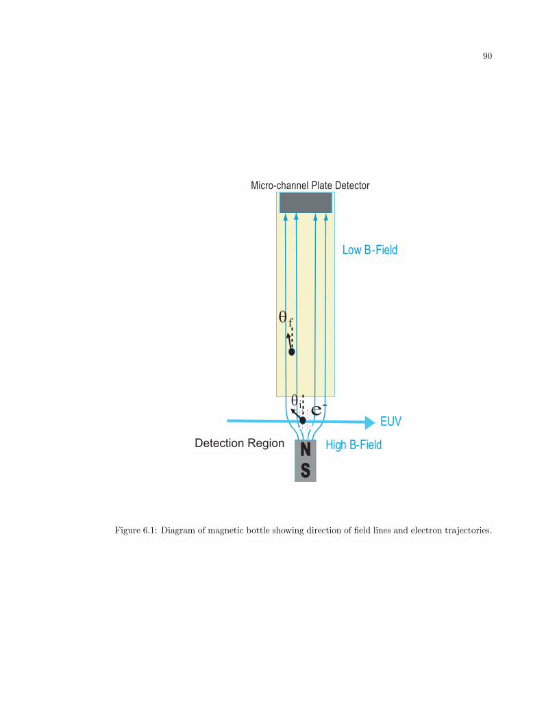
90

High B-Field

Low B-Field

NS

Micro-channel Plate Detector

e-

Detection Region

θi

θf

EUV

Figure 6.1: Diagram of magnetic bottle showing direction of field lines and electron trajectories.

91

even electrons initially travelling in a direction away from the flight tube end up with most of

their velocity redirected along axis. A schematic of the apparatus indicating the magnetic field

is given in Figure 6.1.

The theory of operation of the spectrometer is described in detail by P. Kruit and F. H.

Read.[43] The initial angular momentum of the electron is given by

` = m2v2 sin2 θi/eBi, (6.1)

where m, v, and e are the mass, velocity, and charge of the electron, θi is the initial angle of

the velocity with respect to the time-of-flight axis, and Bi is the initial, strong magnetic field.

From conservation of angular momentum, the final velocity angle of the electron, θf , in the

lower magnetic field, Bf , is given by the relation

sin θf

sin θi= (

Bf

Bi)1/2. (6.2)

If the difference between the initial and final fields is large enough, the final velocity direction

will be along the TOF axis for a range of different initial angles. For example, if Bf/Bi =

10−3, then for the maximum initial angle, θi = 90 degrees, the final angle is given by, θf =

sin−1(Bf/Bi)1/2 = 1.8 degrees. It is important to have a large difference in the initial and final

field so that electrons with the same initial velocity will have the same drift time in the TOF

tube. Also, for the best energy resolution, it is important for the changing-field region to be as

short as possible while remaining in the adiabatic limit. The adiabaticity parameter is defined

by

χ =2πmv

eB2z

|dBz

dz|, (6.3)

which is the fractional change in the field that the electron experiences in one cyclotron orbit.

The design of the spectrometer is shown in Figure 6.2. The spectrometer consists of a

stack of permanent magnets to generate the strong field in the detection region and a flight

tube with a solenoid constructed around it to create a uniform lower field. A cone with a 2 mm

diameter aperture is located before the entrance to the time-of-flight tube to allow differential

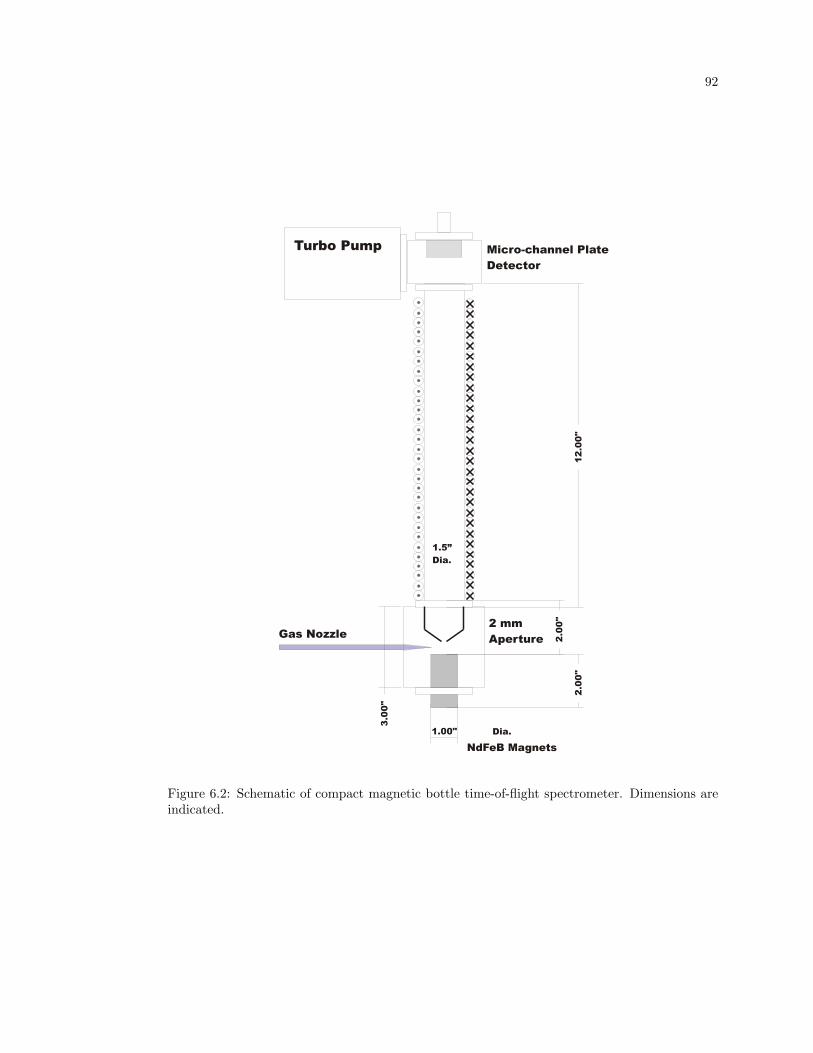
92

Gas Nozzle

NdFeB Magnets

12.0

0"

1.00" Dia.

2.0

0"

2.0

0"

Turbo Pump Micro-channel Plate

Detector

1.5”

Dia.

3.0

0"

2 mm

Aperture

Figure 6.2: Schematic of compact magnetic bottle time-of-flight spectrometer. Dimensions areindicated.

93

pumping and to limit the detection region. At the top of the TOF is a micro-channel plate

(MCP) detector and a 60 L/s turbo pump which evacuates the TOF region to a pressure of

10−6 Torr. A 3 cm long, 150 µm inner-diameter hollow-core glass fiber is used as a gas nozzle

to continuously leak gas into the detection region. Another 60 L/s turbo pump is attached

adjacent to the detection chamber so that the pressure in the detection region does not reach

above ∼ 10−4 Torr with the nozzle on. All of the surfaces in the detection region and TOF tube

are coated with conductive carbon powder to eliminate any charge buildup effects. Also, care

was taken to ensure that all parts were constructed with aluminum or non-magnetic stainless

steel. The MCP detector design is given in Appendix C. The current signal from the detector

is amplified by a 1 GHz Amplifier and Timing Discriminator (EG&G Ortec Model 9327) and

then recorded by a timing board on a PC (ACAM Time Measuring Device Model AM-F1,

manufactured by Acam-messelectronic gmbh Karlsruhe, Germany). The start signal is taken

from an SRS Delay Generator which also provides the trigger for the Pockels cell of the amplifier.

The true start time is obtained by direct detection of scattered photons from the driving laser,

producing a current signal from the MCP detector.

To aid in the design of the spectrometer, the total magnetic field was modelled. The

magnetic field of the permanent magnets are calculated using the equation for the magnetic

scalar potential,[36]

ΦM (x) =14π

∮S

n′ ·M(x′)da′

|x− x′|. (6.4)

The surface integral is evaluated over the top and bottom faces of the magnet. The value of

the magnetization, M, was found by fitting the experimentally measured value of the field on

axis at several distances from the magnet face, shown in figure 6.3. The magnetic field of the

solenoid was calculated using the equation for the magnetic field of a current loop, given in

reference [45], p.112. The solenoid field is then the sum of all the loop fields. The solenoid

parameters are loop radius of 2.05 cm, current of 1 A, and 9 loops/cm with a total length of 30

cm. The solenoid starts 5 cm above the top face of the permanent magnet. The code used for

the calculation is given in Appendix B. Figure 6.4 shows the total magnetic field on axis due to

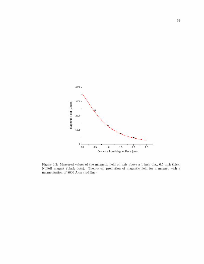
94

0 . 0 0 . 5 1 . 0 1 . 5 2 . 0 2 . 50

1 0 0 0

2 0 0 0

3 0 0 0

4 0 0 0

Magn

etic F

ield (G

auss)

D i s t a n c e f r o m M a g n e t F a c e ( c m )

Figure 6.3: Measured values of the magnetic field on axis above a 1 inch dia., 0.5 inch thick,NdFeB magnet (black dots). Theoretical prediction of magnetic field for a magnet with amagnetization of 8000 A/m (red line).

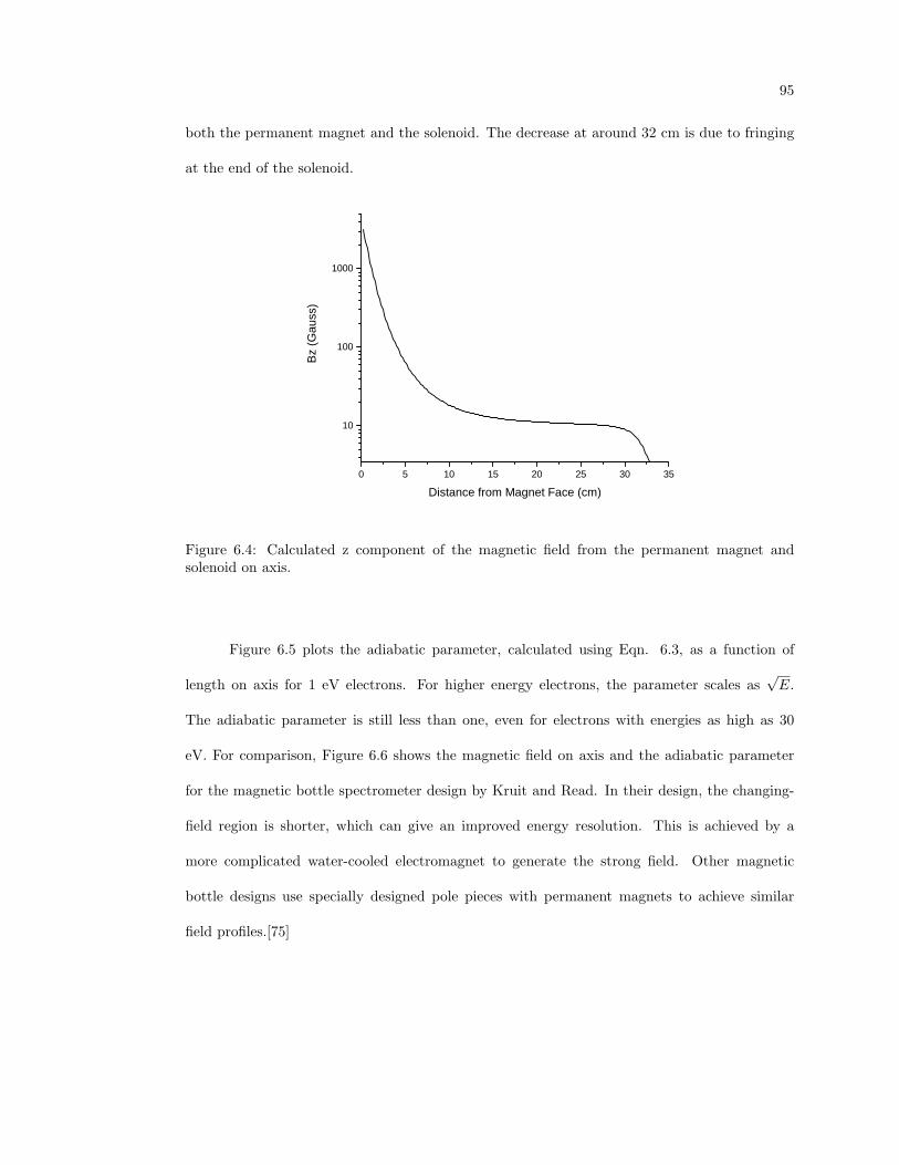
95

both the permanent magnet and the solenoid. The decrease at around 32 cm is due to fringing

at the end of the solenoid.

0 5 1 0 1 5 2 0 2 5 3 0 3 5

1 0

1 0 0

1 0 0 0

Bz (G

auss)

D i s t a n c e f r o m M a g n e t F a c e ( c m )

Figure 6.4: Calculated z component of the magnetic field from the permanent magnet andsolenoid on axis.

Figure 6.5 plots the adiabatic parameter, calculated using Eqn. 6.3, as a function of

length on axis for 1 eV electrons. For higher energy electrons, the parameter scales as√

E.

The adiabatic parameter is still less than one, even for electrons with energies as high as 30

eV. For comparison, Figure 6.6 shows the magnetic field on axis and the adiabatic parameter

for the magnetic bottle spectrometer design by Kruit and Read. In their design, the changing-

field region is shorter, which can give an improved energy resolution. This is achieved by a

more complicated water-cooled electromagnet to generate the strong field. Other magnetic

bottle designs use specially designed pole pieces with permanent magnets to achieve similar

field profiles.[75]

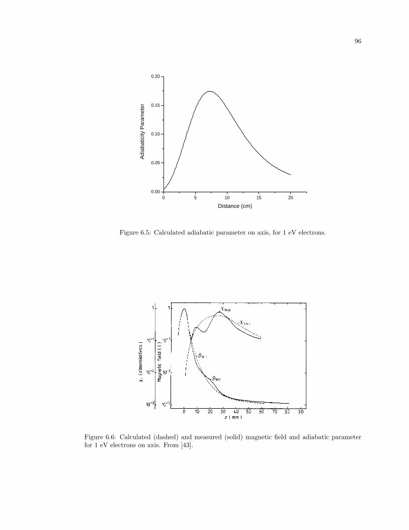
96

0 5 1 0 1 5 2 00 . 0 0

0 . 0 5

0 . 1 0

0 . 1 5

0 . 2 0

Adiab

aticity

Param

eter

D i s t a n c e ( c m )

Figure 6.5: Calculated adiabatic parameter on axis, for 1 eV electrons.

Figure 6.6: Calculated (dashed) and measured (solid) magnetic field and adiabatic parameterfor 1 eV electrons on axis. From [43].

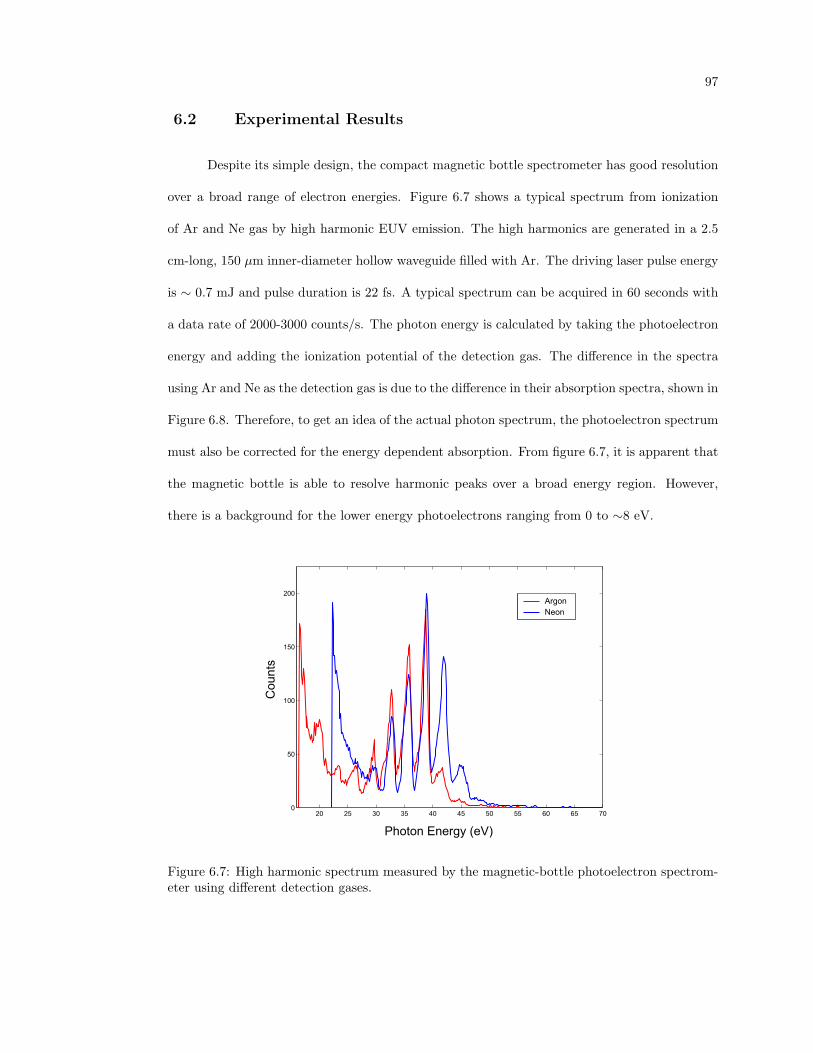
97

6.2 Experimental Results

Despite its simple design, the compact magnetic bottle spectrometer has good resolution

over a broad range of electron energies. Figure 6.7 shows a typical spectrum from ionization

of Ar and Ne gas by high harmonic EUV emission. The high harmonics are generated in a 2.5

cm-long, 150 µm inner-diameter hollow waveguide filled with Ar. The driving laser pulse energy

is ∼ 0.7 mJ and pulse duration is 22 fs. A typical spectrum can be acquired in 60 seconds with

a data rate of 2000-3000 counts/s. The photon energy is calculated by taking the photoelectron

energy and adding the ionization potential of the detection gas. The difference in the spectra

using Ar and Ne as the detection gas is due to the difference in their absorption spectra, shown in

Figure 6.8. Therefore, to get an idea of the actual photon spectrum, the photoelectron spectrum

must also be corrected for the energy dependent absorption. From figure 6.7, it is apparent that

the magnetic bottle is able to resolve harmonic peaks over a broad energy region. However,

there is a background for the lower energy photoelectrons ranging from 0 to ∼8 eV.

20 25 30 35 40 45 50 55 60 65 700

50

100

150

200

Photon Energy (eV)

Cou

nts

ArgonNeon

Figure 6.7: High harmonic spectrum measured by the magnetic-bottle photoelectron spectrom-eter using different detection gases.

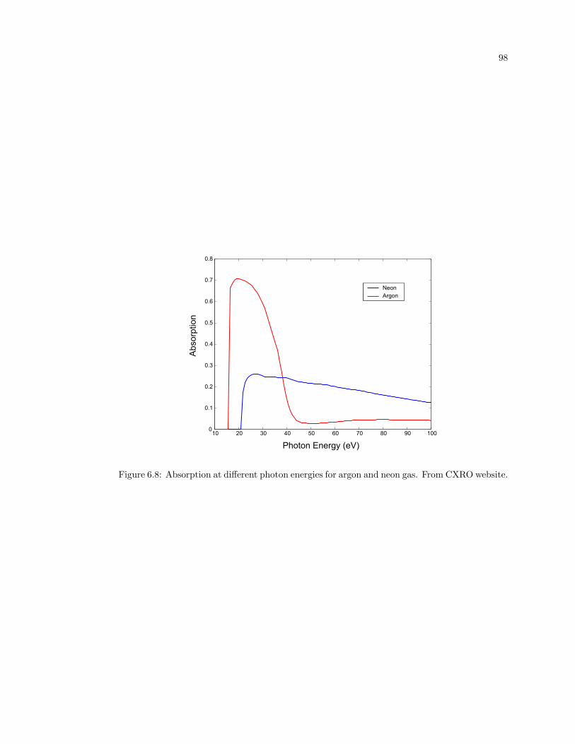
98

10 20 30 40 50 60 70 80 90 1000

0.1

0.2

0.3

0.4

0.5

0.6

0.7

0.8

Photon Energy (eV)

Abs

orpt

ion

NeonArgon

Figure 6.8: Absorption at different photon energies for argon and neon gas. From CXRO website.

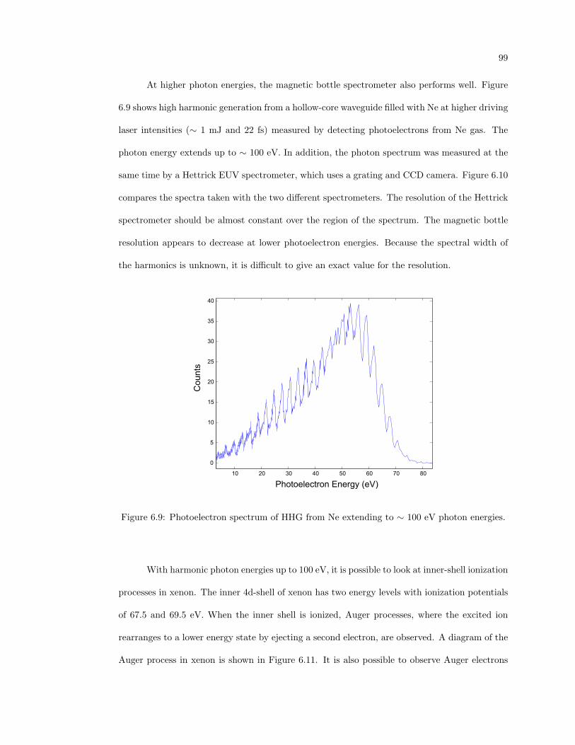
99

At higher photon energies, the magnetic bottle spectrometer also performs well. Figure

6.9 shows high harmonic generation from a hollow-core waveguide filled with Ne at higher driving

laser intensities (∼ 1 mJ and 22 fs) measured by detecting photoelectrons from Ne gas. The

photon energy extends up to ∼ 100 eV. In addition, the photon spectrum was measured at the

same time by a Hettrick EUV spectrometer, which uses a grating and CCD camera. Figure 6.10

compares the spectra taken with the two different spectrometers. The resolution of the Hettrick

spectrometer should be almost constant over the region of the spectrum. The magnetic bottle

resolution appears to decrease at lower photoelectron energies. Because the spectral width of

the harmonics is unknown, it is difficult to give an exact value for the resolution.

10 20 30 40 50 60 70 80

0

5

10

15

20

25

30

35

40

Photoelectron Energy (eV)

Cou

nts

Figure 6.9: Photoelectron spectrum of HHG from Ne extending to ∼ 100 eV photon energies.

With harmonic photon energies up to 100 eV, it is possible to look at inner-shell ionization

processes in xenon. The inner 4d-shell of xenon has two energy levels with ionization potentials

of 67.5 and 69.5 eV. When the inner shell is ionized, Auger processes, where the excited ion

rearranges to a lower energy state by ejecting a second electron, are observed. A diagram of the

Auger process in xenon is shown in Figure 6.11. It is also possible to observe Auger electrons

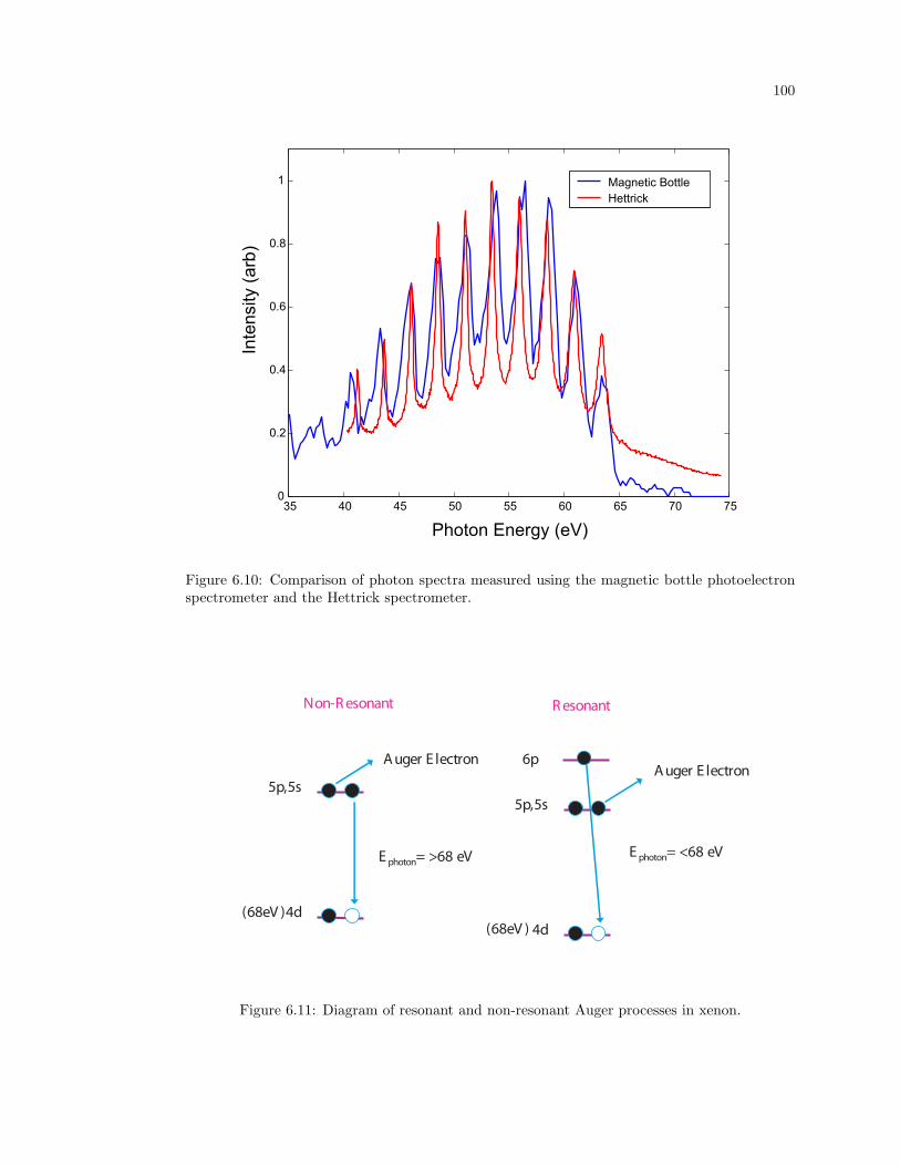
100

35 40 45 50 55 60 65 70 750

0.2

0.4

0.6

0.8

1

Photon Energy (eV)

Inte

nsity

(arb

)

Magnetic BottleHettrick

Figure 6.10: Comparison of photon spectra measured using the magnetic bottle photoelectronspectrometer and the Hettrick spectrometer.

5p,5s

4d(68eV )

A uger E lectron

5p,5s

4d(68eV )

6pA uger E lectron

E photon= >68 eV E photon= <68 eV

R esonantNon-R esonant

Figure 6.11: Diagram of resonant and non-resonant Auger processes in xenon.

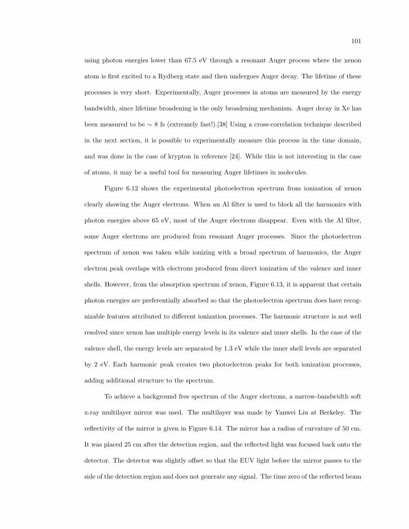
101

using photon energies lower than 67.5 eV through a resonant Auger process where the xenon

atom is first excited to a Rydberg state and then undergoes Auger decay. The lifetime of these

processes is very short. Experimentally, Auger processes in atoms are measured by the energy

bandwidth, since lifetime broadening is the only broadening mechanism. Auger decay in Xe has

been measured to be ∼ 8 fs (extremely fast!).[38] Using a cross-correlation technique described

in the next section, it is possible to experimentally measure this process in the time domain,

and was done in the case of krypton in reference [24]. While this is not interesting in the case

of atoms, it may be a useful tool for measuring Auger lifetimes in molecules.

Figure 6.12 shows the experimental photoelectron spectrum from ionization of xenon

clearly showing the Auger electrons. When an Al filter is used to block all the harmonics with

photon energies above 65 eV, most of the Auger electrons disappear. Even with the Al filter,

some Auger electrons are produced from resonant Auger processes. Since the photoelectron

spectrum of xenon was taken while ionizing with a broad spectrum of harmonics, the Auger

electron peak overlaps with electrons produced from direct ionization of the valence and inner

shells. However, from the absorption spectrum of xenon, Figure 6.13, it is apparent that certain

photon energies are preferentially absorbed so that the photoelectron spectrum does have recog-

nizable features attributed to different ionization processes. The harmonic structure is not well

resolved since xenon has multiple energy levels in its valence and inner shells. In the case of the

valence shell, the energy levels are separated by 1.3 eV while the inner shell levels are separated

by 2 eV. Each harmonic peak creates two photoelectron peaks for both ionization processes,

adding additional structure to the spectrum.

To achieve a background free spectrum of the Auger electrons, a narrow-bandwidth soft

x-ray multilayer mirror was used. The multilayer was made by Yanwei Liu at Berkeley. The

reflectivity of the mirror is given in Figure 6.14. The mirror has a radius of curvature of 50 cm.

It was placed 25 cm after the detection region, and the reflected light was focused back onto the

detector. The detector was slightly offset so that the EUV light before the mirror passes to the

side of the detection region and does not generate any signal. The time zero of the reflected beam

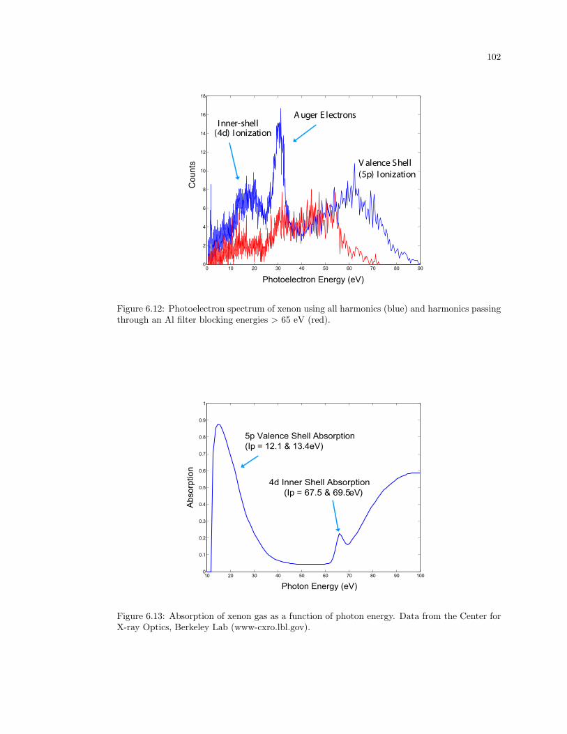
102

0 10 20 30 40 50 60 70 80 900

2

4

6

8

10

12

14

16

18

Photoelectron Energy (eV)

Cou

nts V alence Shell

(5p) Ionization

A uger E lectronsInner-shell

(4d) Ionization

Figure 6.12: Photoelectron spectrum of xenon using all harmonics (blue) and harmonics passingthrough an Al filter blocking energies > 65 eV (red).

10 20 30 40 50 60 70 80 90 1000

0.1

0.2

0.3

0.4

0.5

0.6

0.7

0.8

0.9

1

Photon Energy (eV)

Abs

orpt

ion

5p Valence Shell Absorption(Ip = 12.1 & 13.4eV)

4d Inner Shell Absorption(Ip = 67.5 & 69.5 eV)

Figure 6.13: Absorption of xenon gas as a function of photon energy. Data from the Center forX-ray Optics, Berkeley Lab (www-cxro.lbl.gov).

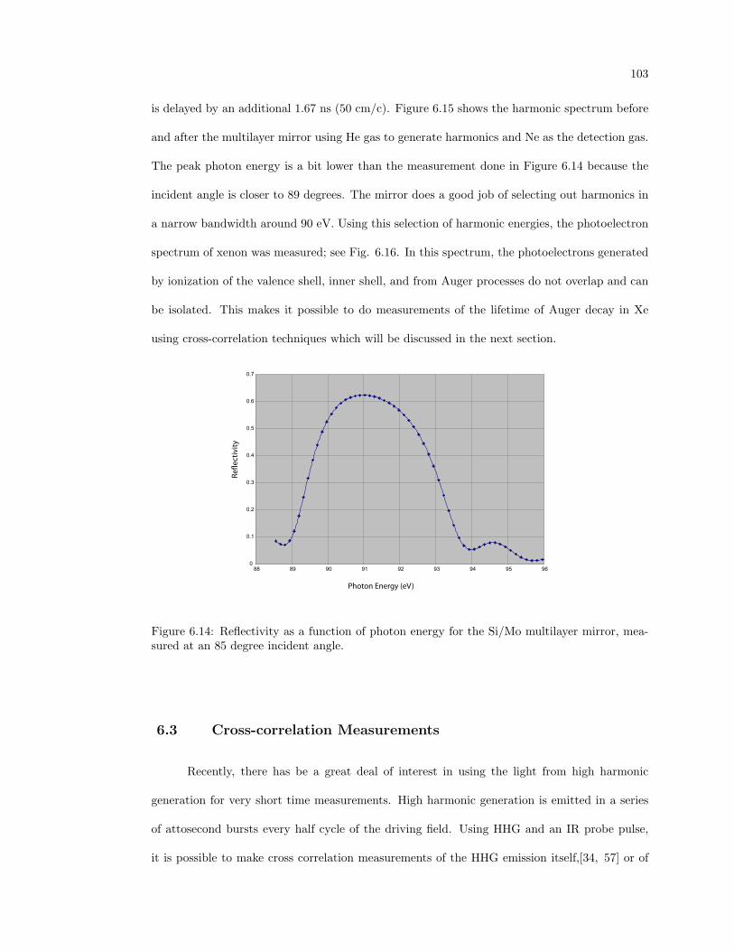
103

is delayed by an additional 1.67 ns (50 cm/c). Figure 6.15 shows the harmonic spectrum before

and after the multilayer mirror using He gas to generate harmonics and Ne as the detection gas.

The peak photon energy is a bit lower than the measurement done in Figure 6.14 because the

incident angle is closer to 89 degrees. The mirror does a good job of selecting out harmonics in

a narrow bandwidth around 90 eV. Using this selection of harmonic energies, the photoelectron

spectrum of xenon was measured; see Fig. 6.16. In this spectrum, the photoelectrons generated

by ionization of the valence shell, inner shell, and from Auger processes do not overlap and can

be isolated. This makes it possible to do measurements of the lifetime of Auger decay in Xe

using cross-correlation techniques which will be discussed in the next section.

0

0.1

0.2

0.3

0.4

0.5

0.6

0.7

88 89 90 91 92 93 94 95 96

Photon Energy (eV)

Ref

lect

ivit

y

Figure 6.14: Reflectivity as a function of photon energy for the Si/Mo multilayer mirror, mea-sured at an 85 degree incident angle.

6.3 Cross-correlation Measurements

Recently, there has be a great deal of interest in using the light from high harmonic

generation for very short time measurements. High harmonic generation is emitted in a series

of attosecond bursts every half cycle of the driving field. Using HHG and an IR probe pulse,

it is possible to make cross correlation measurements of the HHG emission itself,[34, 57] or of

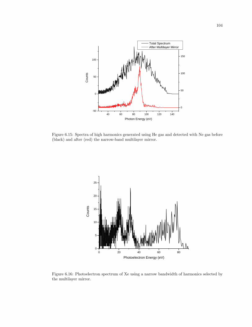
104

4 0 6 0 8 0 1 0 0 1 2 0 1 4 0- 5 0

0

5 0

1 0 0

0

5 0

1 0 0

1 5 0

Coun

ts

P h o t o n E n e r g y ( e V )

T o t a l S p e c t r u m A f t e r M u l t i l a y e r M i r r o r

Figure 6.15: Spectra of high harmonics generated using He gas and detected with Ne gas before(black) and after (red) the narrow-band multilayer mirror.

0 2 0 4 0 6 0 8 00

5

1 0

1 5

2 0

2 5

Coun

ts

P h o t o e l e c t r o n E n e r g y ( e V )

Figure 6.16: Photoelectron spectrum of Xe using a narrow bandwidth of harmonics selected bythe multilayer mirror.

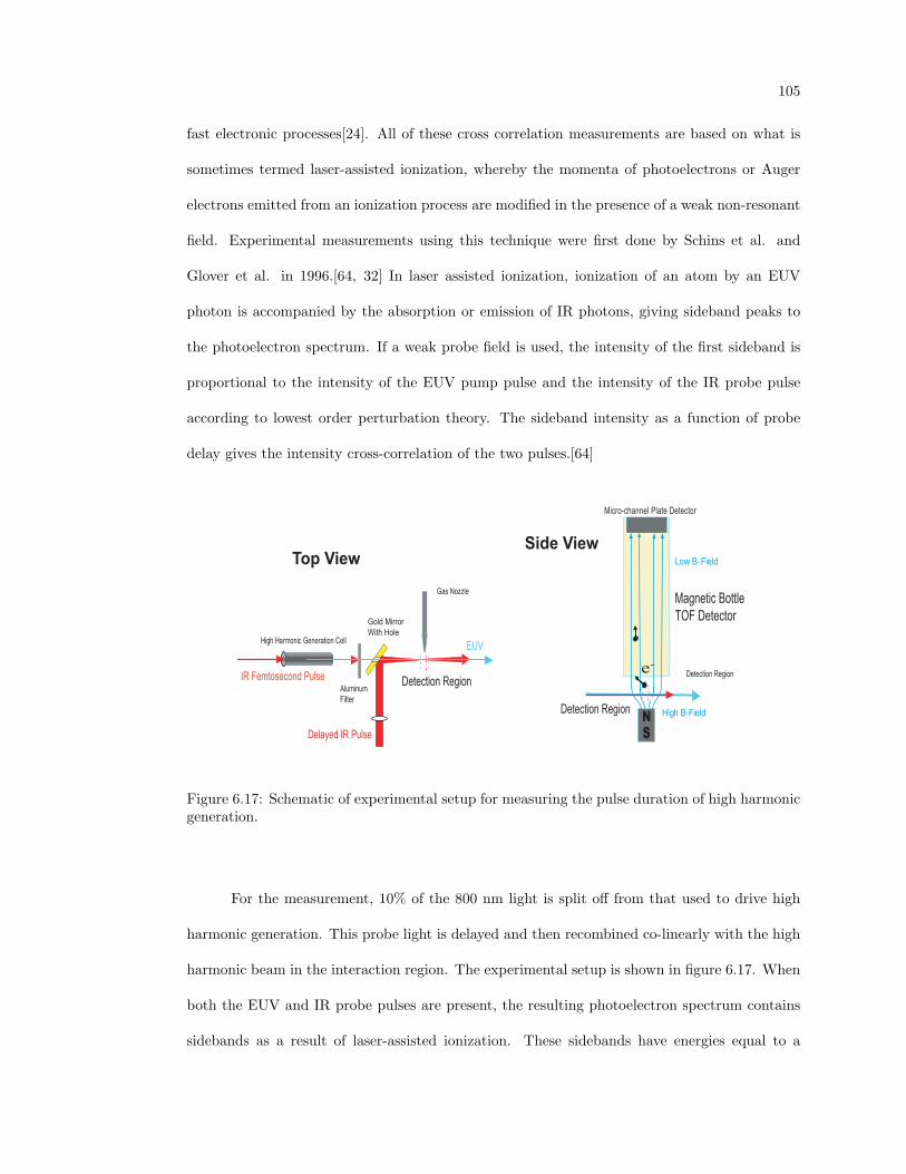
105

fast electronic processes[24]. All of these cross correlation measurements are based on what is

sometimes termed laser-assisted ionization, whereby the momenta of photoelectrons or Auger

electrons emitted from an ionization process are modified in the presence of a weak non-resonant

field. Experimental measurements using this technique were first done by Schins et al. and

Glover et al. in 1996.[64, 32] In laser assisted ionization, ionization of an atom by an EUV

photon is accompanied by the absorption or emission of IR photons, giving sideband peaks to

the photoelectron spectrum. If a weak probe field is used, the intensity of the first sideband is

proportional to the intensity of the EUV pump pulse and the intensity of the IR probe pulse

according to lowest order perturbation theory. The sideband intensity as a function of probe

delay gives the intensity cross-correlation of the two pulses.[64]

AluminumFilter

High Harmonic Generation Cell

IR Femtosecond Pulse

EUV

Gold MirrorWith Hole

Delayed IR Pulse

Gas Nozzle

Detection Region

High B-Field

Low B-Field

Magnetic Bottle TOF Detector

NS

Micro-channel Plate Detector

e-

Top ViewSide View

Detection Region

Detection Region

Figure 6.17: Schematic of experimental setup for measuring the pulse duration of high harmonicgeneration.

For the measurement, 10% of the 800 nm light is split off from that used to drive high

harmonic generation. This probe light is delayed and then recombined co-linearly with the high

harmonic beam in the interaction region. The experimental setup is shown in figure 6.17. When

both the EUV and IR probe pulses are present, the resulting photoelectron spectrum contains

sidebands as a result of laser-assisted ionization. These sidebands have energies equal to a

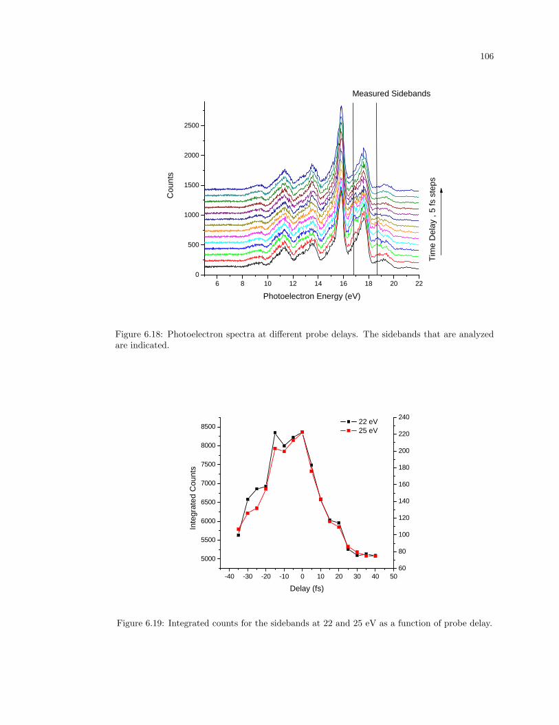
106

6 8 1 0 1 2 1 4 1 6 1 8 2 0 2 20

5 0 0

1 0 0 0

1 5 0 0

2 0 0 0

2 5 0 0

Coun

ts

P h o t o e l e c t r o n E n e r g y ( e V )

Time D

elay ,

5 fs

steps

M e a s u r e d S i d e b a n d s

Figure 6.18: Photoelectron spectra at different probe delays. The sidebands that are analyzedare indicated.

- 4 0 - 3 0 - 2 0 - 1 0 0 1 0 2 0 3 0 4 0 5 0

5 0 0 0

5 5 0 0

6 0 0 0

6 5 0 0

7 0 0 0

7 5 0 0

8 0 0 0

8 5 0 0 2 2 e V 2 5 e V

Integ

rated

Coun

ts

D e l a y ( f s )

6 08 01 0 01 2 01 4 01 6 01 8 02 0 02 2 02 4 0

Figure 6.19: Integrated counts for the sidebands at 22 and 25 eV as a function of probe delay.

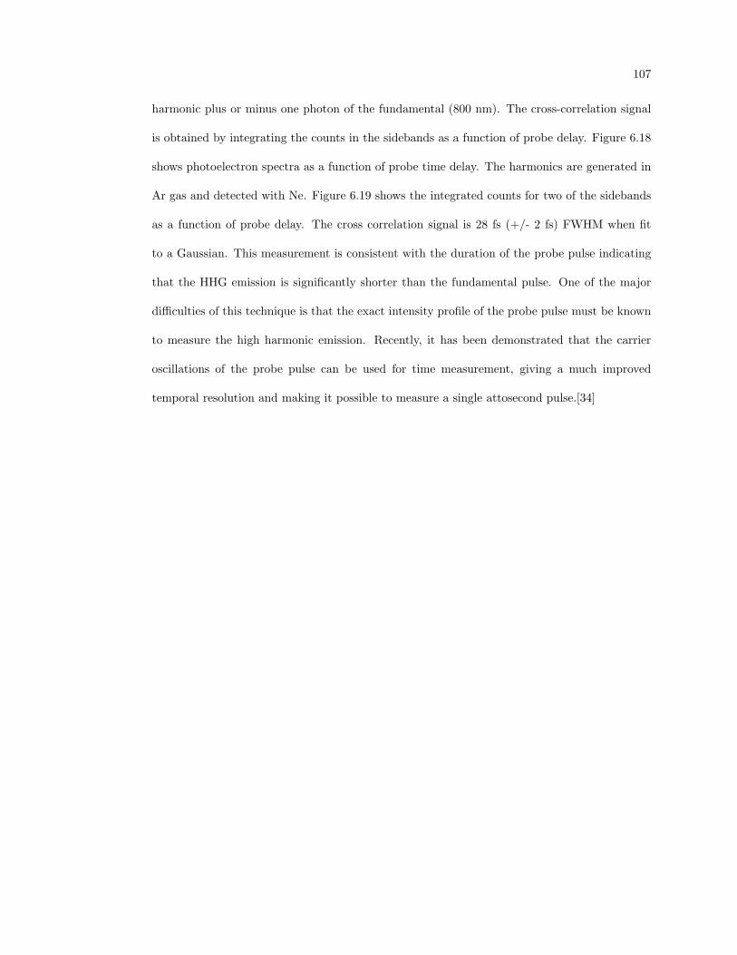
107

harmonic plus or minus one photon of the fundamental (800 nm). The cross-correlation signal

is obtained by integrating the counts in the sidebands as a function of probe delay. Figure 6.18

shows photoelectron spectra as a function of probe time delay. The harmonics are generated in

Ar gas and detected with Ne. Figure 6.19 shows the integrated counts for two of the sidebands

as a function of probe delay. The cross correlation signal is 28 fs (+/- 2 fs) FWHM when fit

to a Gaussian. This measurement is consistent with the duration of the probe pulse indicating

that the HHG emission is significantly shorter than the fundamental pulse. One of the major

difficulties of this technique is that the exact intensity profile of the probe pulse must be known

to measure the high harmonic emission. Recently, it has been demonstrated that the carrier

oscillations of the probe pulse can be used for time measurement, giving a much improved

temporal resolution and making it possible to measure a single attosecond pulse.[34]

Chapter 7

Conclusion

In conclusion, this work applies nonlinear optical techniques to significantly higher pho-

ton energies than before, enhancing the conversion efficiency and opening up the possibility of

generating multi-keV photon energies from high harmonic generation. The ideas in this work

have the potential to greatly increase the number of applications possible using HHG in many

areas of chemistry and biology by making it a practical, efficient, table-top light source. The

enhancements demonstrated in this work are still far from the theoretical limits. Future work on

quasi-phase matching over longer fiber lengths and using shorter modulations should improve the

photon flux from HHG even further. Quasi-phase matching techniques may also provide a means

of generating an enhanced attosecond duration pulse of high harmonic light. Currently, high

harmonic generation is the only method for generating light pulses of durations in the attosec-

ond regime (1 attosecond = 10−18 seconds). Already, initial experiments have been performed

using light from HHG to measure electronic processes on attosecond time scales. Therefore,

the advances demonstrated in this work have the potential to influence both technology and

fundamental science.

Bibliography

[1] G. P. Agrawal. Nonlinear Fiber Optics. Academic Press, San Diego, 3rd edition, 2001.

[2] C. Altucci, T. Starczwski, E. Mevel, C. Wahlstrom, B. Carre, and A. L’Huillier. Journal ofthe Optical Society of America B, 13:148, 1996.

[3] M.V. Ammosov, N.B. Delone, and V.P. Krainov. Tunnel ionization of complex atoms andof atomic ions in an alternating electromagnetic field. Soviet Physics JETP, 64(6):1191,1986.

[4] J.A. Armstrong, N. Bloembergen, J. Ducuing, and P.S. Pershan. Interactions between lightwaves in a nonlinear dielectric. Physical Review A, 127:1918, 1962.

[5] S. Augst, D.D. Meyerhofer, D. Strickland, and S.L. Chin. Laser ionization of noble gasesby coulomb-barrier suppression. JOSA B, 8(4):858–867, 1991.

[6] S. Augst, D. Strickland, D.D. Meyerhofer, S.L. Chin, and J.H. Eberly. Tunneling ionizationof noble gases in a high-intensity laser field. Physical Review Letters, 63(20):2212–2215,1989.

[7] S. Backus, R. Bartels, S. Thompson, R. Dollinger, H. C. Kapteyn, and M. M. Murnane.High-efficiency, single-stage 7-khz high-average-power ultrafast laser system. Optics Letters,26(7):465–467, 2001.

[8] S. Backus, C. Durfee, M.M. Murnane, and H.C. Kapteyn. High power ultrafast lasers.Review of Scientific Instruments, 69(3):1207–1223, 1998.

[9] P. Balcou, P. Salieres, A. L’Huillier, and M. Lewenstein. Generalized phase-matching condi-tions for high harmonics: The role of field-gradient forces. Physical Review A, 55(4):3204–3210, 1997.

[10] R. A. Bartels, A. Paul, H. Green, H. C. Kapteyn, M. M. Murnane, S. Backus, I. P. Christov,Y. W. Liu, D. Attwood, and C. Jacobsen. Generation of spatially coherent light at extremeultraviolet wavelengths. Science, 297(5580):376–378, 2002.

[11] M. Bauer, C. Lei, K. Read, R. Tobey, J. Gland, M. M. Murnane, and H. C. Kapteyn. Directobservation of surface chemistry using ultrafast soft-x- ray pulses. Physical Review Letters,87(2):025501, 2001.

[12] J. D. Bierlein, D. B. Laubacher, J. B. Brown, and C. J. van der Poel. Balanced phasematching in segmented ktiopo4 waveguides. Applied Physics Letters, 56(18):1725–1727,1990.

[13] R. W. Boyd. Nonlinear Optics. Academic Press, San Diego, 2nd edition, 2003.

110

[14] T. Brabec and F. Krausz. Intense few-cycle laser fields: Frontiers of nonlinear optics.Reviews of Modern Physics, 72(2):545–591, 2000.

[15] Z. H. Chang, A. Rundquist, H. W. Wang, M. M. Murnane, and H. C. Kapteyn. Gener-ation of coherent soft x-rays at 2.7 nm using high harmonics. Physical Review Letters,79(16):2967–2970, 1997.

[16] Z. H. Chang, A. Rundquist, H. W. Wang, M. M. Murnane, and H. C. Kapteyn. Temporalphase control of soft-x-ray harmonic emission. Physical Review A, 58(1):R30–R33, 1998.

[17] E.A. Chowdhury, C.P.J. Barty, and B.C. Walker. Nonrelativistic ionization of the l-shellstates in argon by a relativistic 1019 w/cm−2 laser field. Physical Review A, 63:042712,2001.

[18] I. P. Christov. Control of high harmonic and attosecond pulse generation in aperiodicmodulated waveguides. Journal of the Optical Society of America B, 18(12):1877–1881,2001.

[19] I. P. Christov, H. C. Kapteyn, and M. M. Murnane. Quasi-phase matching of high-harmonics and attosecond pulses in modulated waveguides. Optics Express, 7(11):362–367,2000.

[20] I.P. Christov, M.M. Murnane, and H.C. Kapteyn. Generation and propagation of attosecondx-ray pulses in gaseous media. Physical Review A, 57(4):R2285, 1998.

[21] E. Constant, D. Garzella, P. Breger, E. Mevel, C. Dorrer, C. Le Blanc, F. Salin, andP. Agostini. Optimizing high harmonic generation in absorbing gases: Model and experi-ment. Physical Review Letters, 82(8):1668–1671, 1999.

[22] P. B. Corkum. Plasma perspective on strong field multiphoton ionization. Physical ReviewLetters, 71(13):1994–1997, 1993.

[23] D. Descamps, C. Lynga, J. Norin, A. L’Huillier, C. G. Wahlstrom, J. F. Hergott, H. Merdji,P. Salieres, M. Bellini, and T. W. Hansch. Extreme ultraviolet interferometry measurementswith high-order harmonics. Optics Letters, 25(2):135–137, 2000.

[24] M. Drescher, M. Hentschel, R. Kienberger, M. Uiberacker, V. Yakovlev, A. Scrinizi, T. West-erwalbesloh, U. Kleineberg, U. Heinzmann, and F. Krausz. Time-resolved atomic inner-shellspectroscopy. Nature, 419(6909):803–807, 2002.

[25] C. G. Durfee, A. Rundquist, S. Backus, Z. Chang, C. Herne, H. C. Kapteyn, and M. M.Murnane. Guided-wave phase-matching of ultrashort-pulse light. Journal of NonlinearOptical Physics & Materials, 8(2):211–234, 1999.

[26] C. G. Durfee, A. R. Rundquist, S. Backus, C. Herne, M. M. Murnane, and H. C. Kapteyn.Phase matching of high-order harmonics in hollow waveguides. Physical Review Letters,83(11):2187–2190, 1999.

[27] M. M. Fejer, G. A. Magel, D. H. Jundt, and R. L. Byer. Quasi-phase-matched 2nd harmonic-generation - tuning and tolerances. IEEE Journal of Quantum Electronics, 28(11):2631–2654, 1992.

[28] M. Ferray, A. L’Huillier, X. F. Li, L. A. Lompr, G. Mainfray, and C. Manus. Multiple-harmonic conversion of 1064 nm radiation in rare gasses. Journal of Physics B, 21:L31,1987.

[29] M. B. Gaarde, F. Salin, Ph. Balcou, K. J. Schafer, K. C. Kulander, and A. L’Huillier.Spatiotemporal separation of high harmonic radiation into two quantum path components.Physical Review A, 59(2):1367–1373, 1999.

111

[30] E. A. Gibson, A. Paul, N. Wagner, R. Tobey, S. Backus, I. P. Christov, M. M. Murnane,and H. C. Kapteyn. High-order harmonic generation up to 250 ev from highly ionizedargon. Physical Review Letters, 92(3):033001, 2004.

[31] E. A. Gibson, A. Paul, N. Wagner, R. Tobey, D. Gaudiosi, S. Backus, I. P. Christov,A. Aquila, E. M. Gullikson, D. T. Attwood, M. M. Murnane, and H. C. Kapteyn. Co-herent soft x-ray generation in the water window with quasi-phase matching. Science,302(5642):95–98, 2003.

[32] T. E. Glover, R. W. Schoenlein, A. H. Chin, and C. V. Shank. Observation of laser as-sisted photoelectric effect and femtosecond high order harmonic radiation. Physical ReviewLetters, 76(14):2468–2471, 1996.

[33] R. Haight and D. R. Peale. Tunable photoemission with harmonics from subpicosecondlasers. Review of Scientific Instruments, 65(6):1853–1857, 1994.

[34] M. Hentschel, R. Kienberger, Ch. Spielmann, G. A. Reider, N. Milosevic, T. Brabec,P. Corkum, U. Heinzmann, M. Drescher, and F. Krausz. Attosecond metrology. Nature,414(6863):509–513, 2001.

[35] Michael C. Hettrick. In-focus monochromator: Theory and experiment of a new grazingincidence mounting. Applied Optics, 29:4531–4535, 1990.

[36] John David Jackson. Classical Electrodynamics, 3rd Edition. John Wiley & Sons, Inc.,New York, 1999.

[37] J. Javanainen, J.H. Eberly, and Q. Su. Numerical simulations of multiphoton ionizationand above-threshold electron spectra. Physical Review A, 38:3430, 1988.

[38] M. Jurvansuu, A. Kivimaki, and S. Aksela. Inherent lifetime widths of ar 2p−1, kr 3d−1,xe 3d−1, and xe 4d−1 states. Physical Review A, 64:012502–7, 2001.

[39] H. C. Kapteyn, L. B. D. Silva, and R. W. Falcone. Short-wavelength lasers. Proceedingsof the IEEE, 80(3):342, 1992.

[40] R. Kienberger, E. Goulielmakis, M. Uiberacker, A. Baltuska, V. Yakovlev, F. Bammer,A. Scrinzi, T. Westerwalbesloh, U. Kleineberg, U. Heinzmann, M. Drescher, and F. Krausz.Atomic transient recorder. Nature, 427(6977):817–821, 2004.

[41] V.P. Krainov. Ionization rates and energy and angular distributions at the barrier-suppression ionization of complex atoms and atomic ions. Journal of the Optical Societyof America B, 14(2):425, 1997.

[42] J. L. Krause, K. J. Schafer, and K. C. Kulander. High-order harmonic generation fromatoms and ions in the high intensity regime. Physical Review Letters, 68(24):3535, 1992.

[43] P. Kruit and F. H. Read. Magnetic field paralleliser for 2π electron-spectrometer andelectron-image magnifier. Journal of Physics E - Scientific Instruments, 16(4):313–324,1983.

[44] K. C. Kulander, K. J. Schafer, and J. L. Krause. Dynamics of short-pulse excitation,ionization and harmonic conversion. In Super-intense laser-atom physics, 316, pages 95–110. NATO Advanced Science Institutes, 1993.

[45] L. D. Landau, E. M. Lifshitz, and L. P. Pitaevskii. Electrodynamics of Continuous Media,2nd Edition. Reed Educational and Professional Publishing Ltd, Oxford, 1984.

[46] M. Lewenstein, Ph. Balcou, M. Y. Ivanov, and P.B. Corkum. Theory of high-harmonicgeneration of low-frequency laser fields. Physical Review A, 49(3):2117–2132, 1993.

112

[47] M. Lewenstein, P. Salieres, and A. L’Huillier. Phase of the atomic polarization in high-orderharmonic generation. Physical Review A, 52(6):4747–4754, 1995.

[48] A. L’Huillier, M. Lewenstein, P. Salieres, P. Balcou, M. Y. Ivanov, J. Larsson, and C. G.Wahlstrom. High-order harmonic-generation cutoff. Physical Review A, 48(5):R3433–R3436, 1993.

[49] A. R. Libertun, X. Zhang, A. Paul, E. Gagnon, T. Popmintchev, S. Backus, M. M. Murnane,H. C. Kapteyn, and I. P. Christov. Design of fully spatially coherent extreme-ultravioletlight sources. Applied Physics Letters, 84(19):3903–3905, 2004.

[50] E.A.J. Marcatili and R.A. Schmeltzer. Hollow metallic and dielectric waveguides for longdistance optical transmission and lasers. Bell System Technical Journal, 43:1783, 1964.

[51] A. McPherson, G. Gibson, H. Jara, U. Johann, T. S. Luk, I. A. McIntyre, K. Boyer, andC. K. Rhodes. Studies of multiphoton production of vacuum-ultraviolet radiation in therare gasses. Journal of the Optical Society of America B, 4:595–601, 1987.

[52] J. H. Moore, C. C. Davis, and M. A. Coplan. Building scientific apparatus : a practicalguide to design and construction, 2nd edition. Addison-Wesley, Redwood City, CA, 1989.

[53] B. Nikolaus and D. Grishkowsky. 12x pulse compression using optical fibers. AppliedPhysics Letters, 42(1):1–2, 1983.

[54] M. Nisoli, S. De Silvestri, and O. Svelto. Generation of high energy 10 fs pulses by a newpulse compression technique. Applied Physics Letters, 68(20):2793–2795, 1996.

[55] L. Nugent-Glandorf, M. Scheer, D. A. Samuels, A. M. Mulhisen, E. R. Grant, X. M. Yang,V. M. Bierbaum, and S. R. Leone. Ultrafast time-resolved soft x-ray photoelectron spec-troscopy of dissociating br-2. Physical Review Letters, 87(19):193002, 2001.

[56] A. Paul, R. A. Bartels, R. Tobey, H. Green, S. Weiman, I. P. Christov, M. M. Murnane,H. C. Kapteyn, and S. Backus. Quasi-phase-matched generation of coherent extreme-ultraviolet light. Nature, 421(6918):51–54, 2003.

[57] P. M. Paul, E. S. Toma, P. Breger, G. Mullot, F. Auge, Ph. Balcou, H. G. Muller, andP. Agostini. Observation of a train of attosecond pulses from high harmonic generation.Science, 292(5522):1689–1692, 2001.

[58] J. Peatross, M. V. Fedorov, and K. C. Kulander. Intensity-dependent phase-matchingeffects in harmonic generation. Journal of the Optical Society of America B, 12(5):863–870,1995.

[59] S.C. Rae. Ionization-induced defocusing of intense laser pulses in high-pressure gases. OpticsCommunications, 97:25–28, 1993.

[60] J. J. Rocca, C. H. Moreno, M. C. Marconi, and K. Kanizay. Soft-x-ray laser interferometryof a plasma with a tabletop laser and a lloyd’s mirror. Optics Letters, 24:420–422, 1999.

[61] A. Rundquist. Phase-matched generation of coherent, ultrafast x-rays using high harmonics.Ph.d., Washington State University, 1998.

[62] A. Rundquist, C.G. Durfee III, S. Backus, C. Herne, Z. Chang, M.M. Murnane, and H.C.Kapteyn. Phase-matched generation of coherent soft x-rays. Science, 280(5368):1412–1415,1998.

[63] P. Salieres, T. Ditmire, M. Perry, A. L’Huillier, and M. Lewenstein. Angular distributions ofhigh-order harmonics generated by a femtosecond laser. Journal of Physics B, 29(20):4771–4786, 1996.

113

[64] J. M. Schins, P. Breger, P. Agostini, R. C. Constantinescu, H. G. Muller, A. Bouhal,G. Grillon, A. Antonetti, and A. Mysyrowicz. Cross-correlation measurements of femtosec-ond extreme-ultraviolet high-order harmonics. Journal of the Optical Society of AmericaB, 13(1):197–200, 1996.

[65] M. Schnrer, Z. Cheng, M. Hentschel, G. Tempea, P. Klmn, T. Brabec, and F. Krausz.Absorption-limited generation of coherent ultrashort soft-x-ray pulses. Physical ReviewLetters, 83(4):722–725, 1999.

[66] A. Scrinzi, M. Geissler, and T. Brabec. Ionization above the coulomb barrier. PhysicalReview Letters, 83(4):706–709, 1999.

[67] E. Seres, J. Seres, F. Krausz, and C. Spielmann. Generation of coherent soft-x-ray radiationextending far beyond the titanium l edge. Physical Review Letters, 92(16):163002, 2004.

[68] B. Shan and Z. H. Chang. Dramatic extension of the high-order harmonic cutoff by usinga long-wavelength driving field. Physical Review A, 65(1):1804, 2002.

[69] P.L. Shkolnikov, A. Lago, and A.E. Kaplan. Optimal quasi-phase-matching for high-orderharmonic generation in gases and plasmas. Physical Review A, 50(6):R4461, 1994.

[70] C. Spielmann, N. H. Burnett, S. Sartania, R. Koppitsch, M. Schnrer, C. Kan, M. Lenzner,P. Wobrauschek, and F. Krausz. Generation of coherent x-rays in the water window using5-femtosecond laser pulses. Science, 278:661–664, 1997.

[71] C. Spielmann, N. H. Burnett, S. Sartania, R. Koppitsch, M. Schnrer, C. Kan, M. Lenzner,P. Wobrauschek, and F. Krausz. Near-kev coherent x-ray generation with sub-10-fs lasers.IEEE Journal of Selected Topics in Quantum Electronics, 4:249–265, 1998.

[72] G. Tempea and T. Brabec. Nonlinear source for the generation of high-energy few-cycleoptical pulses. Optics Letters, 23(16):1286–1288, 1998.

[73] W. J. Tomlinson, R. H. Stolen, and C. V. Shank. Compression of optical pulses chirpedby self-phase modulation in fibers. Journal of the Optical Society of America B, 1(2):139,1984.

[74] R. Trebino. Frequency-resolved optical gating: the measurement of ultrashort laser pulses.Kluwer Academic, Boston, 2000.

[75] T. Tsuboi, E. Y. Xu, Y. K. Bae, and K. T. Gillen. Magnetic bottle electron spectrometerusing permanent magnets. Review of Scientific Instruments, 59(8):1357–1362, 1988.

[76] J. H. Underwood and E. M. Gullikson. High-resolution, high-flux, user friendly vls beamlineat the als for the 501300 ev energy region. Journal of Electron Spectroscopy and RelatedPhenomena, 92:265–272, 1998.

[77] S. L. Voronov, I. Kohl, J. B. Madsen, J. Simmons, N. Terry, J. Titensor, Q. Wang, andJ. Peatross. Control of laser high-harmonic generation with counterpropagating light.Physical Review Letters, 8713(13):3902, 2001.

[78] N. L. Wagner, E. A. Gibson, T. Popmintchev, I. P. Christov, M. M. Murnane, and H. C.Kapteyn. Self-compression of ultrashort pulses through ionization-induced spatio-temporalreshaping. Physical Review Letters, to be published 2004.

[79] C.G. Wahlstrom, S. Borgstrom, J. Larsson, and S.G. Pettersson. High-order harmonicgeneration in laser-produced ions using a near-infrared laser. Physical Review A, 51:585,1995.

114

[80] C.G. Wahlstrom, J. Larsson, A. Persson, T. Starczewski, S. Svanberg, P. Salires, Ph. Balcou,and A. L’Huillier. High-order harmonic generation in rare gases with an intense short-pulselaser. Phys. Rev. A, 48:4709–4720, 1993.

[81] B. Walker, B. Sheehy, L.F. DiMauro, P. Agostini, K.J. Schafer, and K.C. Kulander. Pre-cision measurement of strong field double ionization of helium. Physical Review Letters,73(9):1227–1230, 1994.

[82] K. Yamane, Z. Zhang, K. Oka, R. Morita, M. Yamashita, and A. Suguro. Optical pulsecompression to 3.4fs in the monocycle region by feedback phase compensation. OpticsLetters, 28(22):2258–2260, 2003.

[83] J. Zhou, J. Peatross, M.M. Murnane, H.C. Kapteyn, and I.P. Christov. Enhanced highharmonic generation using 25 femtosecond laser pulses. Physical Review Letters, 76(5):752–755, 1996.

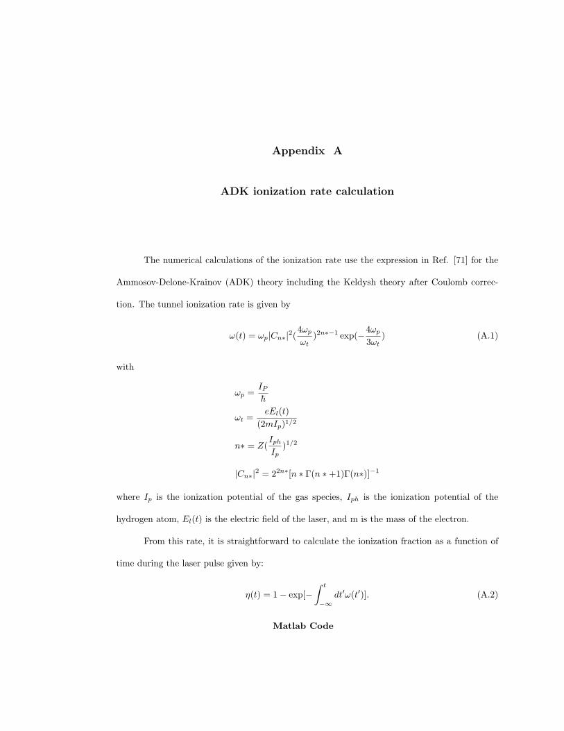
Appendix A

ADK ionization rate calculation

The numerical calculations of the ionization rate use the expression in Ref. [71] for the

Ammosov-Delone-Krainov (ADK) theory including the Keldysh theory after Coulomb correc-

tion. The tunnel ionization rate is given by

ω(t) = ωp|Cn∗|2(4ωp

ωt)2n∗−1 exp(−4ωp

3ωt) (A.1)

with

ωp =IP

h̄

ωt =eEl(t)

(2mIp)1/2

n∗ = Z(Iph

Ip)1/2

|Cn∗|2 = 22n∗[n ∗ Γ(n ∗+1)Γ(n∗)]−1

where Ip is the ionization potential of the gas species, Iph is the ionization potential of the

hydrogen atom, El(t) is the electric field of the laser, and m is the mass of the electron.

From this rate, it is straightforward to calculate the ionization fraction as a function of

time during the laser pulse given by:

η(t) = 1− exp[−∫ t

−∞dt′ω(t′)]. (A.2)

Matlab Code

116

Eion = 0.58065; % Ionization Potential for Argon in a.u.Eion2=27.6/27.21; % 2nd Ionization Potential for Argon in a.u.%Eion = 21.5646/27.21; % Ionization Potential for Neon in a.u.%Eion2=40.1/27.21; % 2nd Ionization Potential for Neon in a.u.

QN = 1./sqrt(2*Eion);QN2 = 2./sqrt(2*Eion2);Ain = 5.0E14; % Peak intensity in W/cm2Ain = sqrt(Ain/3.51E16); % Electric field amplitude

Tpul = 30.; % Pulse FWHM in fsTpul = Tpul*1E-15*4.1322E16;Tf = Tpul*0.84932;wo = 0.05695;TT = 2.*pi/wo;Nx = 10000; % Number of time stepsHT = 4.*Tf/Nx;for i=1:Nx T = i*HT; E(i)=Ain*exp(-(T-2.0*Tf)^2/Tf^2)*cos(wo*(T-2*Tf)); Int(i)=(Ain*exp(-(T-2.0*Tf)^2/Tf^2))^2;end

N(1)=1.;N1(i)=0.;N2(1)=0.;T(1)=0.;Rint=0.;for i=1:Nx-1 T(i+1) = i*HT; F = abs(E(i))+1.E-30; C2=2^(2*QN)/(QN*gamma(QN+1)*gamma(QN)); C22=2^(2*QN2)/(QN2*gamma(QN2+1)*gamma(QN2)); Rate1(i)=Eion*C2*(4.0*Eion*sqrt(2.0*Eion)/F)^(2.0*QN-1.0)*... exp(-4.0*Eion*sqrt(2.0*Eion)/(3.0*F)); Rate2(i)=Eion2*C22*(4.0*Eion2*sqrt(2.0*Eion2)/F)^(2.0*QN2-1.0)*... exp(-4.0*Eion2*sqrt(2.0*Eion2)/(3.0*F)); Rint=Rint+Rate1(i)*HT; N(i+1)=exp(-Rint); % Number of Neutrals N1(i+1)=1.-N(i)-N2(i); % Number of Single Ions N2(i+1)= N2(i)+Rate2(i)*N1(i)*HT; % Number of Double Ions Rate1(i)=Rate1(i)*N(i); Rate2(i)=Rate2(i)*N1(i);end

Neutral=1-N;Ion1=N1;Ion2=N2;T=(T-2*Tf)/TT*2.67; % Convert to fs

Appendix B

Magnetic Field Calculations

The calculation of the magnetic field of the magnetic-bottle spectrometer in Mathematica

is given on the following pages.

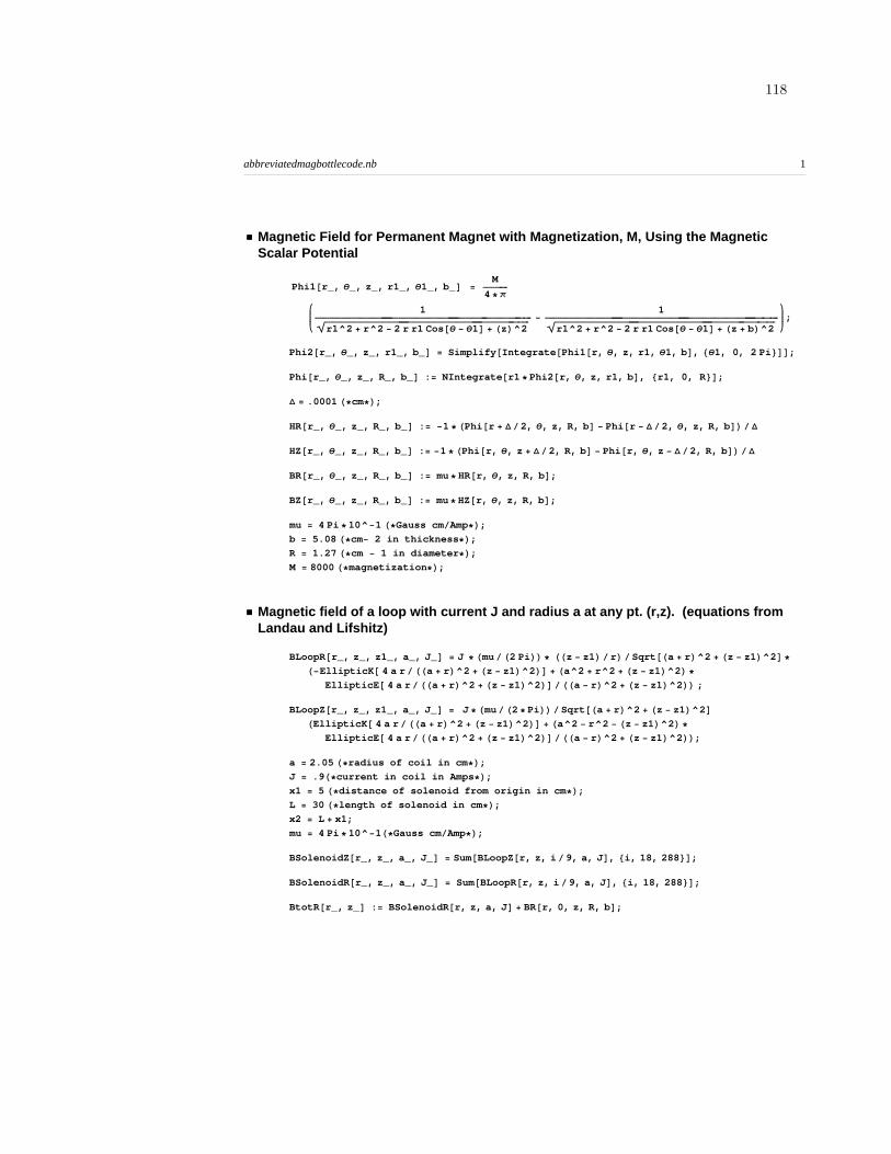
118

ü Magnetic Field for Permanent Magnet with Magnetization, M, Using the Magnetic Scalar Potential

Phi1@r_, θ_, z_, r1_, θ1_, b_D =M

4 ∗ π

i

kjjjjj

1è!!!!!!!!!!!!!!!!!!!!!!!!!!!!!!!!!!!!!!!!!!!!!!!!!!!!!!!!!!!!!!!!!!!!!!!!!!!!!!!!!!!!!!!!!

r1^2 + r^2 − 2 r r1 Cos@θ − θ1D + HzL^2−

1è!!!!!!!!!!!!!!!!!!!!!!!!!!!!!!!!!!!!!!!!!!!!!!!!!!!!!!!!!!!!!!!!!!!!!!!!!!!!!!!!!!!!!!!!!!!!!!!!

r1^2 + r^2 − 2 r r1 Cos@θ − θ1D + Hz + bL^2

y

{zzzzz;

Phi2@r_, θ_, z_, r1_, b_D = Simplify@Integrate@Phi1@r, θ, z, r1, θ1, bD, 8θ1, 0, 2 Pi<DD;

Phi@r_, θ_, z_, R_, b_D := NIntegrate@r1 ∗ Phi2@r, θ, z, r1, bD, 8r1, 0, R<D;

∆ = .0001 H∗cm∗L;

HR@r_, θ_, z_, R_, b_D := −1 ∗HPhi@r + ∆ ê2, θ, z, R, bD − Phi@r − ∆ê2, θ, z, R, bDLê ∆

HZ@r_, θ_, z_, R_, b_D := −1 ∗HPhi@r, θ, z + ∆ê2, R, bD − Phi@r, θ, z − ∆ ê2, R, bDLê∆

BR@r_, θ_, z_, R_, b_D := mu ∗ HR@r, θ, z, R, bD;

BZ@r_, θ_, z_, R_, b_D := mu ∗ HZ@r, θ, z, R, bD;

mu = 4 Pi ∗ 10^−1 H∗Gauss cmêAmp∗L;b = 5.08 H∗cm− 2 in thickness∗L;R = 1.27 H∗cm − 1 in diameter∗L;M = 8000 H∗magnetization∗L;

ü Magnetic field of a loop with current J and radius a at any pt. (r,z). (equations from Landau and Lifshitz)

BLoopR@r_, z_, z1_, a_, J_D = J ∗HmuêH2 PiLL∗ HHz − z1LêrLê Sqrt@Ha + rL^2 + Hz − z1L^2D∗

H−EllipticK@ 4 a rêHHa + rL^2 + Hz − z1L^2LD + Ha^2 + r^2 + Hz − z1L^2L∗

EllipticE@ 4 a rêHHa + rL^2 + Hz − z1L^2LDêHHa − rL^2 + Hz − z1L^2LL ;

BLoopZ@r_, z_, z1_, a_, J_D = J ∗HmuêH2 ∗ PiLLê Sqrt@Ha + rL^2 + Hz − z1L^2DHEllipticK@ 4 a rêHHa + rL^2 + Hz − z1L^2LD + Ha^2 − r^2 − Hz − z1L^2L∗

EllipticE@ 4 a rêHHa + rL^2 + Hz − z1L^2LDêHHa − rL^2 + Hz − z1L^2LL;

a = 2.05 H∗radius of coil in cm∗L;J = .9H∗current in coil in Amps∗L;x1 = 5 H∗distance of solenoid from origin in cm∗L;L = 30 H∗length of solenoid in cm∗L;x2 = L + x1;mu = 4 Pi ∗ 10^−1H∗Gauss cmêAmp∗L;

BSolenoidZ@r_, z_, a_, J_D = Sum@BLoopZ@r, z, iê9, a, JD, 8i, 18, 288<D;

BSolenoidR@r_, z_, a_, J_D = Sum@BLoopR@r, z, i ê9, a, JD, 8i, 18, 288<D;

BtotR@r_, z_D := BSolenoidR@r, z, a, JD + BR@r, 0, z, R, bD;

abbreviatedmagbottlecode.nb 1

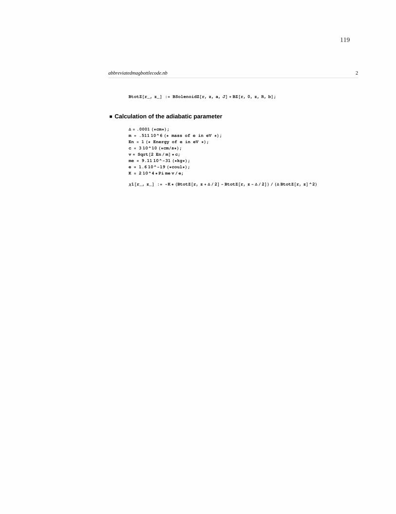
119

BtotZ@r_, z_D := BSolenoidZ@r, z, a, JD + BZ@r, 0, z, R, bD;

ü Calculation of the adiabatic parameter

∆ = .0001 H∗cm∗L;m = .511 10^6 H∗ mass of e in eV ∗L;En = 1 H∗ Energy of e in eV ∗L;c = 3 10^10 H∗cmês∗L;v = Sqrt@2 Enê mD∗ c;me = 9.11 10^−31 H∗kg∗L;e = 1.6 10^−19 H∗coul∗L;K = 2 10^4 ∗ Pi me v êe;

χ1@r_, z_D := −K ∗HBtotZ@r, z + ∆ê2D − BtotZ@r, z − ∆ê2DLêH∆ BtotZ@r, zD^2L

abbreviatedmagbottlecode.nb 2

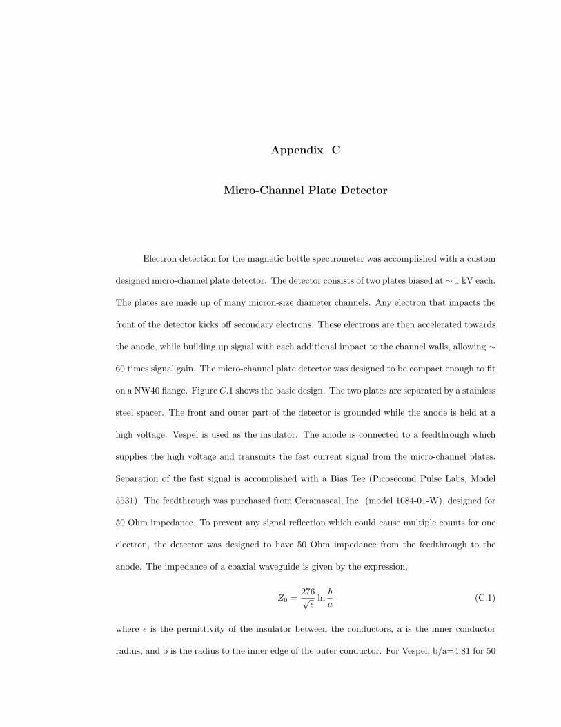
Appendix C

Micro-Channel Plate Detector

Electron detection for the magnetic bottle spectrometer was accomplished with a custom

designed micro-channel plate detector. The detector consists of two plates biased at ∼ 1 kV each.

The plates are made up of many micron-size diameter channels. Any electron that impacts the

front of the detector kicks off secondary electrons. These electrons are then accelerated towards

the anode, while building up signal with each additional impact to the channel walls, allowing ∼

60 times signal gain. The micro-channel plate detector was designed to be compact enough to fit

on a NW40 flange. Figure C.1 shows the basic design. The two plates are separated by a stainless

steel spacer. The front and outer part of the detector is grounded while the anode is held at a

high voltage. Vespel is used as the insulator. The anode is connected to a feedthrough which

supplies the high voltage and transmits the fast current signal from the micro-channel plates.

Separation of the fast signal is accomplished with a Bias Tee (Picosecond Pulse Labs, Model

5531). The feedthrough was purchased from Ceramaseal, Inc. (model 1084-01-W), designed for

50 Ohm impedance. To prevent any signal reflection which could cause multiple counts for one

electron, the detector was designed to have 50 Ohm impedance from the feedthrough to the

anode. The impedance of a coaxial waveguide is given by the expression,

Z0 =276√

εln

b

a(C.1)

where ε is the permittivity of the insulator between the conductors, a is the inner conductor

radius, and b is the radius to the inner edge of the outer conductor. For Vespel, b/a=4.81 for 50

121

Ohm impedance.[52] Figure C.2 shows the detailed dimensions of all the parts of the detector.

Anode2000 V

Micro-channel Plates

VespelInsulator

0 V

Figure C.1: MCP detector design. The micro-channel plates are in dark blue. The anode isbiased at 2 kV and is insulated from the grounded stainless steel housing.

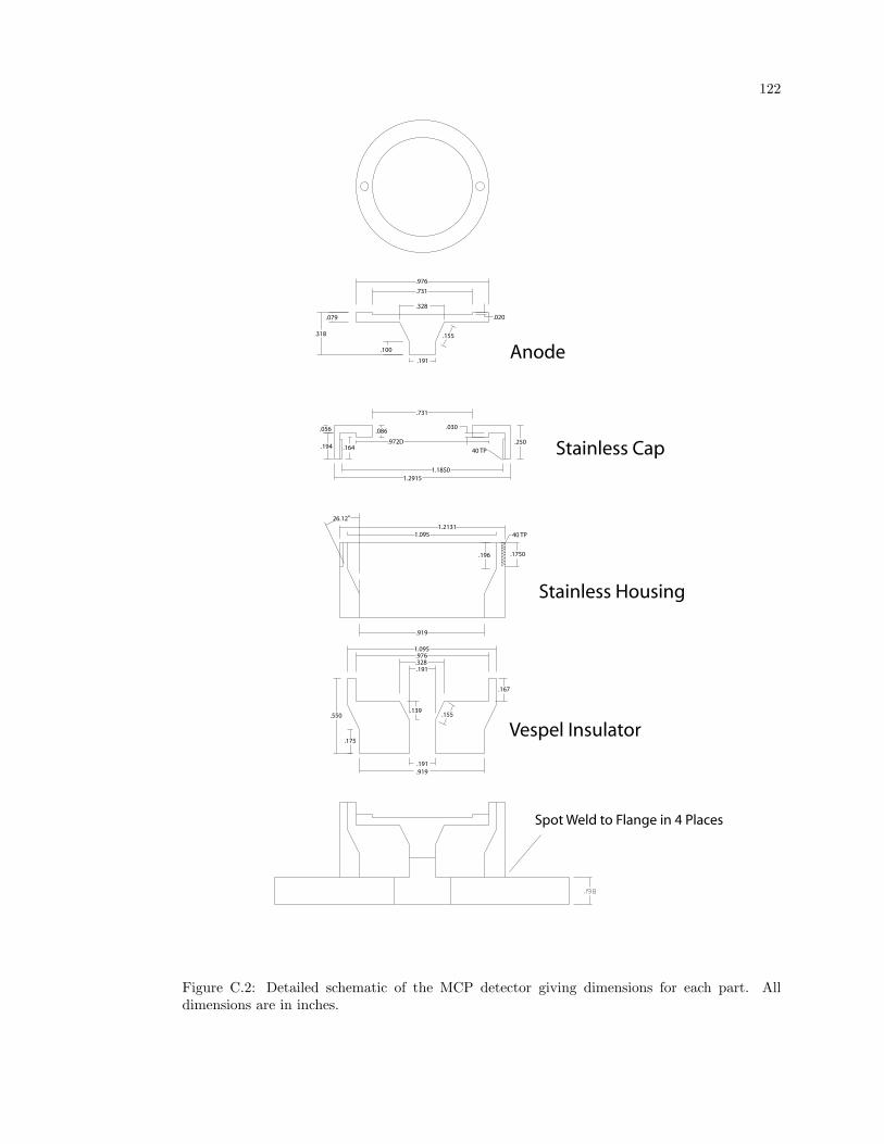
122

Spot Weld to Flange in 4 Places

Vespel Insulator

Stainless Housing

Stainless Cap

Anode

.976

.731

.328

.191

.079

.318

.100

.155

.020

.731

.056

.194

.086.030

.250

1.18501.2915

.164.972D

40 TP

1.0951.2131

26.12o

.196 .1750

40 TP

.919

1.095.976.328.191

.167

.155.139

.550

.175

.191

.919

Figure C.2: Detailed schematic of the MCP detector giving dimensions for each part. Alldimensions are in inches.