query optimization: sorting & joining · example: sql query step 3 step 3: transform initial...

Query Optimization: Sorting & JoiningCS 377: Database Systems

CS 377 [Spring 2016] - Ho

Recap: Query Processing• Some database

operations are expensive

• Performance can be improved by being “smart”

• RA expressions can be optimized via heuristics

• Cost-based optimization to determine “best” query plan

queryoutput

query parser andtranslator

evaluation engine

relational-algebraexpression

execution plan

optimizer

data statisticsabout data

Figure 12.1 from Database System Concepts book


Example: SQL Query Step 1Step 1: Convert SQL query into a parse tree

http://www.mathcs.emory.edu/~cheung/Courses/554/Syllabus/5-query-opt/intro.html



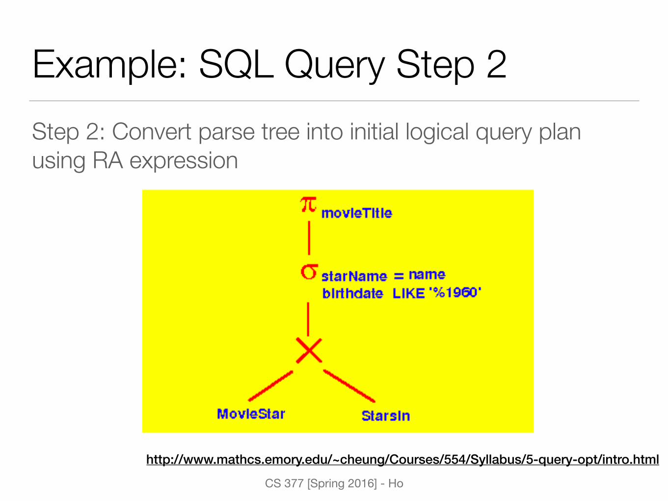
Example: SQL Query Step 2Step 2: Convert parse tree into initial logical query plan using RA expression




Example: SQL Query Step 3Step 3: Transform initial plan into optimal query plan using some measure of cost to determine which plan is better




Example: SQL Query Step 4Step 4: Select physical query operator for each relational algebra operator in the optimal query plan




Recap: Catalog InformationDatabase maintains statistics about each relation

• Size of file: number of tuples [nr], number of blocks [br], tuple size [sr], number of tuples or records per block [fr], etc.

• Information about indexes and indexing attributes

• Attribute values - number of distinct values [V(att, r)]

• Selection cardinality - expected size of selection given value [SC(att, r)]

• …


Recap: Cost-based OptimizationSELECT algorithms

• Linear search

• Binary search

• Index search

Different costs depending on the file organization and indexes


Sorting• One of the primary algorithms used for query processing

• ORDER BY

• DISTINCT

• JOIN

• Relations that fit in memory — use techniques like quicksort, merge sort, bubble sort

• Relations that don’t fit in memory — external sort-merge


External Sort-Merge Algorithm• Problem: Sort r records, stored in b file blocks with a total

memory space of M blocks

• Create sorted runs with i = 0

• Read M blocks of relation into memory

• Sort the in-memory blocks

• Write sorted data to run Ri, increment i


External Sort-Merge Algorithm (2)• Merge the sorted runs: merge subfiles until 1 remains

• Select the first record in sort order from each of the buffers

• Write the record to the output

• Delete the record from the buffer page, and read the next block if empty

• Total cost: br(2dlogM�1(br/M)e+ 1)


Example: External Merge Sort


ga d 31c 33b 14e 16r 16d 21m 3p 2d 7a 14

initialrelation

create

2419Sort fragments of

file in memory using internal sort

— where each run size is the

size of the block

For this example, use block size =

3 tuples

run 1

run 2

run 3

run 4


Example: External Merge Sort (2)


ga d 31c 33b 14e 16r 16d 21m 3p 2d 7a 14

a 19d 31g 24

b 14c 33e 16

d 21m 3r 16

a 14d 7p 2

initialrelation

createruns

mergepass–1

runs runs

2419

Once each run is sorted, we will

merge two runs together at a time

merge 1

merge 2




ga d 31c 33b 14e 16r 16d 21m 3p 2d 7a 14

a 19b 14c 33d 31e 16g 24

a 14d 7d 21m 3p 2r 16

a 19d 31g 24

b 14c 33e 16

d 21m 3r 16

a 14d 7p 2

initialrelation

createruns

mergepass–1

mergepass–2

runs runs

2419

Another layer of sorted runs, so again merge 2

runs at a time…




ga d 31c 33b 14e 16r 16d 21m 3p 2d 7a 14

a 14a 19b 14c 33d 7d 21d 31e 16g 24m 3p 2r 16

a 19b 14c 33d 31e 16g 24

a 14d 7d 21m 3p 2r 16

a 19d 31g 24

b 14c 33e 16

d 21m 3r 16

a 14d 7p 2

initialrelation

createruns

mergepass–1

mergepass–2

runs runssortedoutput

2419


JOIN• One of the most time-consuming operations

• EQUIJOIN & NATURAL JOIN varieties are most prominent — focus on algorithms for these

• Two way join: join on two files

• Multi-way joins: joins involving more than two files


JOIN PerformanceFactors that affect performance

• Tuples of relation stored physically together

• Relations sorted by join attribute

• Existence of indexes


JOIN Algorithms• Several different algorithms to implement joins

• Nested loop join

• Nested-block join

• Indexed nested loop join

• Sort-merge join

• Hash-join

• Choice is based on cost estimate


Example: Bank Schema• Join depositor and customer tables

• Catalog information for both relations:

• ncustomer = 10000

• fcustomer = 25 => bcustomer = 10000/25 = 400

• ndepositor = 5000

• fdepositor = 50 => bdepositor = 5000/50 = 100

• V(cname, depositor) = 2500 (each customer on average has 2 accounts)

• Cname in depositor is a foreign key of customer


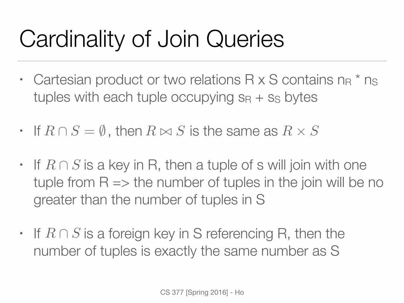
Cardinality of Join Queries• Cartesian product or two relations R x S contains nR * nS

tuples with each tuple occupying sR + sS bytes

• If , then is the same as

• If is a key in R, then a tuple of s will join with one tuple from R => the number of tuples in the join will be no greater than the number of tuples in S

• If is a foreign key in S referencing R, then the number of tuples is exactly the same number as S

R \ S = ; R ./ S R⇥ S

R \ S

R \ S


Cardinality of Join Queries (2)• If and A is not a key of R or S there are two

estimates that can be used

• Assume every tuple in R produces tuples in the join, number of tuples estimated:

• Assume every tuple in S produces tuples in the join, number of tuples estimated:

• Lower of two estimates is probably more accurate

R \ S = {A}

nR ⇤ ns

V (A, s)

nR ⇤ ns

V (A, r)


Example: Cardinality of Join• Estimate the size of

• Assuming no foreign key:

• V(cname, depositor) = 2500 => 5000 * 10000 / 2500 = 20,000

• V(cname, customer) = 10000 =>5000 * 10000 / 10000 = 5000

• Since cname in depositor is foreign key of customer, the size is exactly ndepositor = 5000

Depositor ./ Customer


Nested Loop Join• Default (brute force) algorithm

• Requires no indices and can be used with any join condition

• Algorithm:for each tuple tr in r do for each tuple ts in s do test pair (tr, ts) to see if condition satisfied if satisfied, output (tr, ts) pair

• R is the outer relation and S is the inner relation


Nested Loop Join Cost• Expensive as it examines every pair of tuples in the two

relations

• If smaller relation fits entirely in main memory, use that relation as inner relation

• Worst case: only enough memory to hold one block of each relation, estimated cost is nr * bs + br

• Best case: smaller relation fits in memory, estimated cost is br + bs disk access


Example: Nested Loop Join• Worst case memory scenario:

• Depositor as outer relation: 5000 * 400 + 1000 = 2,000,100 I/Os

• Customer as outer relation: 10000 * 100 + 400 = 1,000,400 I/Os

• Best case memory scenario (depositor fits in memory)

• 100 + 400 = 500 I/Os


Nested-Block Join• Instead of individual tuple basis, join one block at a time together

• Algorithm:for each block in r do for each block in s do use nested loop join algorithm on blocks to output matching pairs

• Worst case: each block in the inner relation s is only read once for each block in the outer relation, so estimated cost is br * bs + br

• Best case: same as nested loop with cost br + bs


Nested-Block vs Nested Loop JoinAssume worst memory case

• Nested loop join with depositor as inner relation: 10000 * 100 + 400 = 1,000,400 I/Os

• Nested-block join with depositor as inner relation: 400 * 100 + 400 = 40400 I/Os

What if a disk speed is 360K I/Os per hour?

• Nested loop join ~= 2.78 hours

• Nested-block join ~= 0.11 hours

A very small change can make a huge

difference in speed!


Indexed Nested-Loop Join• Index is available on inner loop’s join attribute — use index to

compute the join

• Algorithm: for each tuple tr in r do retrieve tuples from s using index search

• Worst case: buffer only has space for one page of r and one page of index, estimated cost is br + nr * c (c is cost of single selection on s using join condition)

• If indices available on both relations, use one with fewer tuples as outer relation


Example: Index Nested Loop Join• Assume customer has primary B+-tree index on customer

name, which contains 20 entries in each node

• Since customer has 10,000 tuples, height of tree is 4

• Using depositor as outer relation, estimated cost: 100 + 5000 * (4 + 1) = 25,100 disk accesses

• Block nested-loop join cost: 100 * 400 + 100 = 40,100 I/Os

• Cost is lower with index nested loop than block nested-loop join


Sort-Merge Join• Sort the relations based on the join

attributes (if not already sorted)

• Merge similar to the external sort-merge algorithm with the main difference in handling duplicate values in the join attribute — every pair with same value on join attribute must be matched

a 3b 1d 8

13df 7

m 5q 6

a Ab Gc Ld Nm B

a1 a2 a1 a3pr ps

r

s



Sort-Merge Join (2)• Can only be used for equijoins and natural joins

• Each tuple needs to be read only once, and as a result, each block is also read only once cost = sorting cost + br + bs

• If one relation is sorted, and other has secondary B+-tree index on join attribute, hybrid merge-joins are possible


Hash-Join• Applicable for equijoins and natural joins

• A hash function, h, is used to partition tuples of both relations into sets that have same hash value on the join attributes

• Tuples in the corresponding same buckets just need to be compared with one another and not with all the other tuples in the other buckets


Example: Hash-Join

Disk

R

S

(3,j) !(0,j) !

(0,a) !(0,a) !

(3,b) !!

(5,b) !!

(0,a) !(0,j) !

Disk

R1

S1

S2

R2

(0,a) !(0,a) !

(0,j) !!

(3,j) !(3,b) !

(0,a) !(0,j) !

(5,b) !!

(5,b) !!

Step 1: Use hash function to partition into B buckets


Example: Hash-Join (2)

Disk

R

S

(3,j) !(0,j) !

(0,a) !(0,a) !

(3,b) !!

(5,b) !!

(0,a) !(0,j) !

Disk

R1

S1

S2

R2

(0,a) !(0,a) !

(0,j) !!

(3,j) !(3,b) !

(0,a) !(0,j) !

(5,b) !!

(5,b) !!

Step 2: Join matching buckets


Hash-Join Algorithm• Partitioning phase

• 1 block for reading and M-1 blocks for hashed partitions

• Hash R tuples into k buckets (partitions)

• Hash S tuples into k buckets (partitions)

• Joining phase (nested block join for each pair of partitions)

• M-2 blocks for R partition, 1 block for S partition


Hash-Join Algorithm• Hash function h and the number of buckets are chosen

such that each bucket should fit in memory

• Recursive partitioning required if number of buckets is greater than number of pages M of memory

• Hash-table overflow occurs if each bucket does not fit in memory


Hash-Join Cost• If recursive partitioning is not required:

• Partitioning phase: 2bR + 2bS

• Joining phase: bR + bS

• Total: 3bR + 3bS

• If recursive partitioning is required:

• Number of passes required to partition:

• Total cost:2(bR + bS)dlogM�1(bS)� 1e+ bR + bS

dlogM�1(bS)� 1e


Example: Hash-Join• Assume memory size is 20 blocks

• What is cost of joining customer and depositor?

• Since depositor has less total blocks, we will use it to partition into 5 buckets, each of size 20 blocks

• Customer is also partitioned into 5 buckets, each of size 80 blocks

• Total cost: 3(100 + 400) = 1500 block transfers


Hybrid Hash-Join• Useful when memory sizes are relatively large and the

smallest relation is bigger than memory

• Idea: Keep first partition in memory to avoid disk I/O for reading and writing the first block

• Assume we have a slightly larger memory size of 25 blocks (compared to previous example) - keep the first partition of depositor in memory (20 blocks)

• Cost: 3(80 + 320) + 20 + 80 = 1300 block transfers


Hash Join vs Sorted Join• Sorted join advantages

• Good if input is already sorted, or need output to be sorted

• Not sensitive to data skew or bad hash functions

• Hash join advantages

• Can be cheaper due to hybrid hashing

• Dependent on size of smaller relation — good for different relation sizes

• Good if input already hashed or need output hashed


Complex Join• What about joins with conjunctive (AND) conditions?

• Compute the result of one of the simpler joins

• Final result consists of tuples in intermediate results that satisfy remaining conditions

• Test these conditions as tuples are generated

• What about joins with disjunctive (OR) conditions?

• Compute as the union of the records in individual joins


Example: Complex JoinWhat if we did a join on loan, depositor, and customer?

• Strategy 1: Compute depositor joins customer and then use that to compute the join with loans

• Strategy 2: Compute loan joins depositor first then use that to join with customer


Example: Complex Join (2)What if we did a join on loan, depositor, and customer?

• Strategy 3: Perform pair of joins at once, build an index on loan for lID and on customer for cname

• For each tuple t in depositor, lookup corresponding tuples in customer and corresponding tuples in loan

• Each tuple of depositor is examined exactly once


PROJECT Algorithms• Extract all tuples from R with only attributes in attribute

list of projection operator & remove tuples

• By default, SQL does not remove duplicates (unless DISTINCT keyword is included)

• Duplicate elimination

• Sorting

• Hashing (duplicates in same bucket)


Aggregation AlgorithmsSimilar to duplicate elimination

• Sort or hash to group same tuples together

• Apply aggregate functions to each group


Set Operation Algorithms• CARTESIAN PRODUCT

• Nested loop - expensive and should avoid if possible

• UNION, INTERSECTION, SET DIFFERENCE

• Sort-merge

• Hashing


Query Processing Recap

SQL Query RA Plan Optimized RA Plan Execution

Declarative user query

Translate to RA expression

Find logically equivalent but

more efficient RA expression

Select physical algorithm with

lowest IO cost to execute the plan


DBMS’s Query Execution Plan• Most commercial RDBMS can produce the query

optimizer’s execution plan to try to understand the decision made by the optimizer

• Common syntax is EXPLAIN <SQL query> (used by MySQL)

• Good DBAs (database administrators) understand query optimizers VERY WELL!


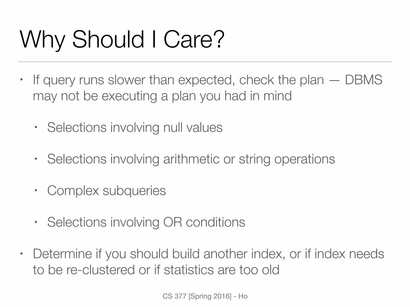
Why Should I Care?• If query runs slower than expected, check the plan — DBMS

may not be executing a plan you had in mind

• Selections involving null values

• Selections involving arithmetic or string operations

• Complex subqueries

• Selections involving OR conditions

• Determine if you should build another index, or if index needs to be re-clustered or if statistics are too old


Query Tuning Guidelines• Minimize the use of DISTINCT — don’t need if duplicates are

acceptable or if answer already has a key

• Minimize use of GROUP BY and HAVING

• Consider DBMS use of index when using math

• E.age = 2 * D.age might only match index on E.age

• Consider using temporary tables to avoid “double-dipping” into a large table

• Avoid negative searches (can’t utilize indexes)


Query Optimization: Recap• External sort-merge

• JOIN algorithms

• Nested loop join

• Nested-block join

• Indexed nested-loop join

• Sort-merge join

• Hash-join

• Other operation algorithms (PROJECT, SET, Aggregate)

query optimization: sorting & joining · example: sql query step 3 step 3: transform initial...

Documents