querying disjunctive databases in … · querying disjunctive databases ... one of the major...
TRANSCRIPT
This material is based upon work supported by the National Science Foundation under Grant #0083127
QUERYING DISJUNCTIVE DATABASESIN POLYNOMIAL TIME
by
Lars E. Olson
A thesis submitted to the faculty ofBrigham Young University
in partial fulfillment of the requirements for the degree of
Master of Science
Department of Computer Science
Brigham Young University
August, 2003

Copyright © 2003 Lars Olson
All Rights Reserved

BRIGHAM YOUNG UNIVERSITY
GRADUATE COMMITTEE APPROVAL
of a thesis submitted by
Lars Olson
This thesis has been read by each member of the following graduate committee and bymajority vote has been found to be satisfactory.
____________________________ ______________________________Date David W. Embley, Chair
____________________________ ______________________________Date Yiu-Kai Dennis Ng
____________________________ ______________________________Date Aurel Cornell
BRIGHAM YOUNG UNIVERSITY
As chair of the candidate’s graduate committee, I have read the thesis of Lars Olson in itsfinal form and have found that (1) its format, citations, and bibliographical style areconsistent and acceptable and fulfill university and department style requirements; (2) itsillustrative materials including figures, tables, and charts are in place; and (3) the finalmanuscript is satisfactory to the graduate committee and is ready for submission to theuniversity library.
____________________________ ______________________________Date David W. Embley, Committee Chairman
Accepted for the Department ______________________________David W. Embley, Graduate Coordinator
Accepted for the College ______________________________G. Rex Bryce, Associate Dean,College of Physical and Mathematical Sciences
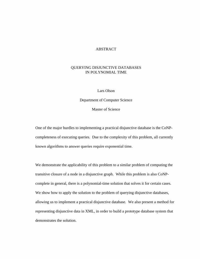
ABSTRACT
QUERYING DISJUNCTIVE DATABASESIN POLYNOMIAL TIME
Lars Olson
Department of Computer Science
Master of Science
One of the major hurdles to implementing a practical disjunctive database is the CoNP-
completeness of executing queries. Due to the complexity of this problem, all currently
known algorithms to answer queries require exponential time.
We demonstrate the applicability of this problem to a similar problem of computing the
transitive closure of a node in a disjunctive graph. While this problem is also CoNP-
complete in general, there is a polynomial-time solution that solves it for certain cases.
We show how to apply the solution to the problem of querying disjunctive databases,
allowing us to implement a practical disjunctive database. We also present a method for
representing disjunctive data in XML, in order to build a prototype database system that
demonstrates the solution.
-vi-
Table of Contents
1 Introduction . . . . . . . . . . . . . . . . . . . . . . . . . . . . . . . . . . . . . . . . . . . . . . . . . . . . . . 1
2 Related Work . . . . . . . . . . . . . . . . . . . . . . . . . . . . . . . . . . . . . . . . . . . . . . . . . . . . . 5
3 The Data Model . . . . . . . . . . . . . . . . . . . . . . . . . . . . . . . . . . . . . . . . . . . . . . . . . . . 7
3.1 Physical Implementation and Mapping to XML Data . . . . . . . . . . . . . . . . 7
3.2 Conversion from XML to a Disjunctive Graph . . . . . . . . . . . . . . . . . . . . 11
4 Query Complexity Issues . . . . . . . . . . . . . . . . . . . . . . . . . . . . . . . . . . . . . . . . . . . 17
4.1 Algorithms . . . . . . . . . . . . . . . . . . . . . . . . . . . . . . . . . . . . . . . . . . . . . . . . 17
4.2 Foundations for a Polynomial-Time Solution . . . . . . . . . . . . . . . . . . . . . 19
4.3 Path-connections and Reachability . . . . . . . . . . . . . . . . . . . . . . . . . . . . . 23
4.4 Simulation of the New Algorithm . . . . . . . . . . . . . . . . . . . . . . . . . . . . . . 28
4.5 Polynomial Running Time . . . . . . . . . . . . . . . . . . . . . . . . . . . . . . . . . . . . 35
5 Analysis and Results . . . . . . . . . . . . . . . . . . . . . . . . . . . . . . . . . . . . . . . . . . . . . . 39
6 Conclusions, Limitations, and Future Work . . . . . . . . . . . . . . . . . . . . . . . . . . . . 47
6.1 Summary . . . . . . . . . . . . . . . . . . . . . . . . . . . . . . . . . . . . . . . . . . . . . . . . . 47
6.2 Limitations and Future Work . . . . . . . . . . . . . . . . . . . . . . . . . . . . . . . . . . 47
Bibliography . . . . . . . . . . . . . . . . . . . . . . . . . . . . . . . . . . . . . . . . . . . . . . . . . . . . . . . . . . . 53
-vii-
List of Figures
1 An example disjunctive graph . . . . . . . . . . . . . . . . . . . . . . . . . . . . . . . . . . . . . . . . 6
2 Sample XML file containing a <Disj> tag . . . . . . . . . . . . . . . . . . . . . . . . . . . . . . 8
3 Disjunctive graph representing XML from Figure 2 . . . . . . . . . . . . . . . . . . . . . . . 8
4 Sample XML file containing a representation of a subset of the cross-product . 10
5 Alternate usage of the <Disj> tag . . . . . . . . . . . . . . . . . . . . . . . . . . . . . . . . . . . 11
6 Sample GEDCOM XML document . . . . . . . . . . . . . . . . . . . . . . . . . . . . . . . . . . . 12
7 DOM tree for the document in Figure 6 . . . . . . . . . . . . . . . . . . . . . . . . . . . . . . . 12
8 Graph from Figure 7 after transforming node names . . . . . . . . . . . . . . . . . . . . . . 13
9 Graph from Figure 8 after adding edge names . . . . . . . . . . . . . . . . . . . . . . . . . . . 14
10 Graph from Figure 9 after adding disjunctive edges . . . . . . . . . . . . . . . . . . . . . . 16
11 Algorithm ComputeClosure, which ensures that edges are added in order . . . . . 17
12 Algorithm AddEdge, the modified algorithm from [LYY95] . . . . . . . . . . . . . . . 18
13 Graph to demonstrate why the number of paths is exponential . . . . . . . . . . . . . . 21
14 Graph that does not satisfy the conditions of Theorem 1 . . . . . . . . . . . . . . . . . . . 27
15 Graph that does not satisfy the conditions of Theorem 1, but would still work with
the modified algorithm . . . . . . . . . . . . . . . . . . . . . . . . . . . . . . . . . . . . . . . . . . . . . 28
16 Example disjunctive graph . . . . . . . . . . . . . . . . . . . . . . . . . . . . . . . . . . . . . . . . . . 29
17 Comparison of query algorithms without computing path information . . . . . . . . 41
18 Comparison of query algorithms including path information . . . . . . . . . . . . . . . 42
19 Comparison of query algorithms after adding disjunctions . . . . . . . . . . . . . . . . . 43
20 Comparison of query algorithms on randomly generated data . . . . . . . . . . . . . . 45
-1-
Chapter 1
Introduction
In some data-storage applications, uncertain or contradictory data can occur. One
such application is genealogy: sometimes, for a single person we may find multiple
possible birth dates, multiple names, or even multiple family relations such as father or
mother. Many of these people lived long ago, and it may not ever be possible to ascertain
the correct values. One possibility, of course, is that contradictory data for one person
might indicate two separate people rather than one, but this might not be true for other
cases. Assuming the data refers to the same person, then, one possible policy would be to
store all the uncertain values, rather than choosing one and discarding the others.
This kind of data represents disjunctive data (i.e. data with an OR semantics, as in
“a or b or ...”). Introducing disjunctive data also introduces some extra logic that normal
databases do not provide. For example, suppose we are working with a genealogy data
model, such as GEDCOM [GED02], that associates individuals with a number of events,
which contain dates and places. Suppose further that for a given individual we have two
possible birth dates and places: 3 Jan 1904 at Provo, Utah, and 4 Jan 1904 at Payson,
Utah. Thus we have to create two event records, and create a disjunction to link the
individual with the two possible event records. However, suppose we query for the birth
year of this person—regardless of which event record is correct, we know that the year is
1904. In other words, for every possible interpretation of this data, the birth year for this
individual is 1904.
-2-
Since normal databases only have one possible interpretation, they have no need
for this kind of query functionality. Can regular databases be extended to allow for
queries with multiple interpretations? The answer is “yes,” but unfortunately, it has been
proven that answering queries on disjunctive databases is, in general, a CoNP-complete
problem [IV89]. Interesting special cases, however, may have polynomial-time solutions.
As we shall see in this thesis, the problem of computing transitive closures in
disjunctive graphs is highly similar to the problem we wish to solve. The general
transitive-closure problem is CoNP-complete, but under certain conditions it can be
solved in polynomial time [LYY95]. Can a similar approach be used in disjunctive
databases, and will these “certain conditions” still apply? As we will show in this thesis,
if we interpret values in the database as nodes in a graph, and relationships between
values as edges (with relationships to uncertain values represented as disjunctive edges),
then the database becomes a disjunctive graph, and computing the transitive closure of a
node in this graph will return all related values that appear in every interpretation of the
database.
This is close, but not quite what we want. For example, suppose one of the values
returned is the number 20. What does this 20 represent? Is it the person’s age at some
event? Is it a part of a date, or the page number of a source reference? To answer these
questions, we need to know not only the values, but the relationships used to reach these
values and how the relationships combine to represent them.
Unfortunately, as we shall see in this thesis, even in a graph in which the
polynomial-time algorithm from [LYY95] can be applied, the number of possible paths
-3-
between a pair of nodes is exponential. Thus, in order to keep a polynomial running time,
we must limit the paths we check to those paths that will help answer a query. However,
even limiting our search is not enough—we have to use an algorithm that makes a
stronger guarantee than the [LYY95] algorithm: not only that the values returned are
always reachable in any possible interpretation, but also that they are always reachable
through a given path in any possible interpretation. This thesis describes an extension to
the [LYY95] algorithm that makes these guarantees and still only requires polynomial
time.
We present the contribution of this thesis as follows. Chapter 2 describes work
that has previously been done in areas related to this problem, including why this work
has not fully solved this problem. It also introduces the concept of disjunctive graphs,
and the problem of solving the transitive closure of nodes in these graphs. Chapter 3
explains our representation of disjunctive data in XML. Chapter 4 introduces the
algorithms we use to answer queries on disjunctive data, demonstrates how the
algorithms work on a sample query, and proves that the algorithms run in polynomial
time. Chapter 5 analyzes the performance of a prototype database and query engine that
implement the algorithms. Chapter 6 presents our conclusions and enumerates several
open questions for possible future research.

-4-
1This, of course, assumes that P … NP. We make this assumption for all similar claimsthroughout the thesis.
-5-
Chapter 2
Related Work
Disjunctive databases have been examined in a few other publications, most
notably in [IV89] where it is proved that answering queries is a CoNP-complete problem,
meaning that all known algorithms for calculating the correct answer require exponential
time.1 [AG85] and [KW85] explain how database updates take on different meanings in
the presence of incomplete data (including disjunctive data). [AG85] also explains how
these updates work in context of three possible models of representing incomplete data.
[IV89] also describes a certain set of queries that can be solved in polynomial time,
although these queries require us to mark the attributes in the database under which
disjunctions can occur and those under which disjunctions cannot occur. The authors of
[IV89] describe criteria to determine when a query is intractable and when it can be
solved in polynomial time, depending on the marks of these attributes and how they
combine in a query. Since we wish to allow disjunctions in any part of the database, this
type of query analysis is insufficient.
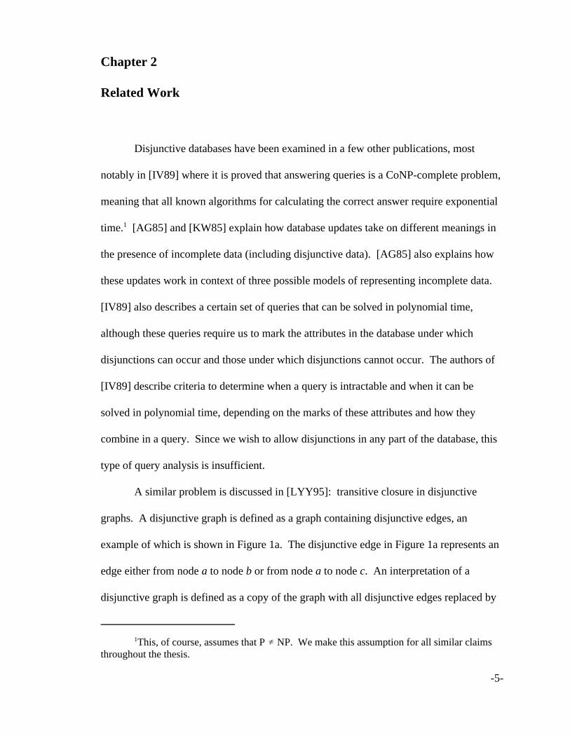
A similar problem is discussed in [LYY95]: transitive closure in disjunctive
graphs. A disjunctive graph is defined as a graph containing disjunctive edges, an
example of which is shown in Figure 1a. The disjunctive edge in Figure 1a represents an
edge either from node a to node b or from node a to node c. An interpretation of a
disjunctive graph is defined as a copy of the graph with all disjunctive edges replaced by
-6-
a
b
c
d
a
b
c
d
a
b
c
d
(a)
(b)
(c)
a
b
c
(d)
Figure 1: (a) An example disjunctive graph, (b),(c) its two interpretations, (d) an edge witha disjunctive tail.
one of the possible edges it represents. Figures 1b and 1c show the two possible
interpretations of the graph in Figure 1a. Since each disjunctive edge represents at least
two possible simple edges, it is easy to show that for a graph with n disjunctive edges,
there are at least 2n possible interpretations.
The transitive closure of a node a is defined as the set of nodes that are always
reachable from a in any interpretation. In Figure 1a, for example, the transitive closure of
node a is {a, d}. Since the number of possible interpretations is exponential, we cannot
determine this answer in polynomial time by simply calculating the intersection of
reachable nodes in every interpretation. This problem is also CoNP-complete in general;
however, [LYY95] gives an algorithm that will compute the answer in polynomial time if
all the disjunctive edges have disjunctions only in the head of the edge, rather than in the
tail. The edge in Figure 1d, for example, has a disjunctive tail, and thus the algorithm
would not work on a graph containing this edge.
-7-
Chapter 3
The Data Model
3.1 Physical Implementation and Mapping to XML Data
The prototype built for our work uses an XML-based database system. In
particular, we use as a database backend the University of Wisconsin’s Shore database
[SHORE] with its Niagara XML interface [NIAGARA] [TDCZ00], which uses
Apache.org’s Xerces C++ XML parser [XERCES]. These technologies are not
necessarily required for representing disjunctive data, nor is XML the only valid
approach. The underlying theory should be applicable to any data-storage system.
We chose XML in order to be compatible with newer standards such as
GEDCOM 6.0 [GED02]. These XML data formats must be slightly modified to include
some way to label sets of data values as disjunctions in order to be usable with our query
algorithm. Such a modification should, ideally, minimize the changes required to adapt
currently existing data for this type of database, and, at the same time, should also be as
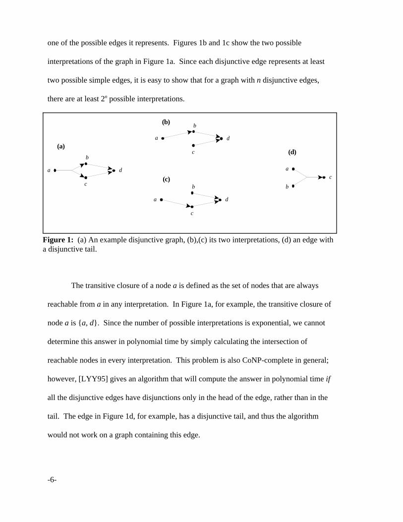
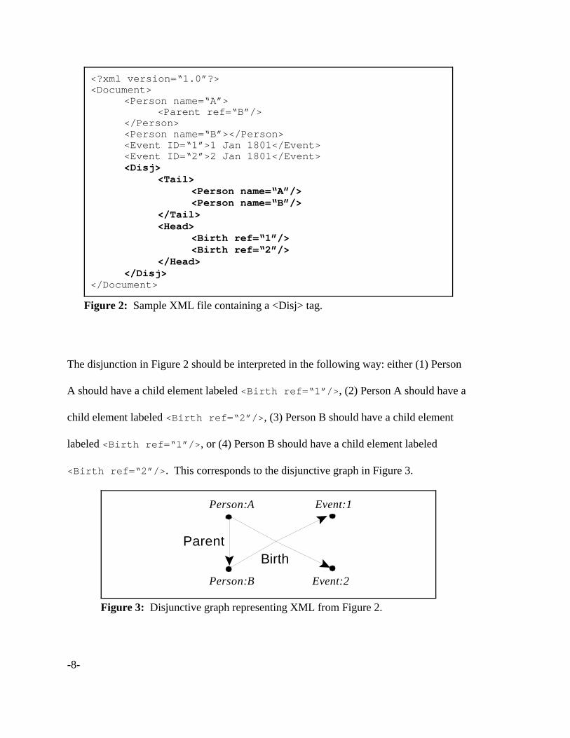
easy as possible for a human reader to understand. For this purpose we introduce
<Disj>, <Tail>, and <Head> tags to a standard XML document, as Figure 2 shows.
We assume that “name” is a key attribute for Person, “ID” is a key attribute for Event, the
“ref” attribute of Birth is a foreign key referencing Event, and the “ref” attribute of Parent
is a foreign key referencing Person.
-8-
<?xml version=“1.0”?><Document>
<Person name=“A”><Parent ref=“B”/>
</Person><Person name=“B”></Person><Event ID=“1”>1 Jan 1801</Event><Event ID=“2”>2 Jan 1801</Event><Disj>
<Tail><Person name=“A”/><Person name=“B”/>
</Tail><Head>
<Birth ref=“1”/><Birth ref=“2”/>
</Head></Disj>
</Document>
Figure 2: Sample XML file containing a <Disj> tag.
Person:A
Birth
Person:B
Event:1
Event:2
Parent
Figure 3: Disjunctive graph representing XML from Figure 2.
The disjunction in Figure 2 should be interpreted in the following way: either (1) Person
A should have a child element labeled <Birth ref=“1”/>, (2) Person A should have a
child element labeled <Birth ref=“2”/>, (3) Person B should have a child element
labeled <Birth ref=“1”/>, or (4) Person B should have a child element labeled
<Birth ref=“2”/>. This corresponds to the disjunctive graph in Figure 3.

-9-
For simple edges (edges without a disjunction), we store the head of the edge as a
child element of the tail of the edge. In Figure 3, for example, the edge labeled “Parent”
corresponds to the <Parent ref=“B”/> element in Figure 2.
In the most general case, we use a <Disj> tag for each disjunctive edge in the
graph. These tags appear as child elements of the root element of the document, and each
should have a <Tail> child element and a <Head> child element. The children of the
<Tail> element, called the tail nodes, should reference other records in the document,
and the children of the <Head> element, called the head nodes, should be elements that
would otherwise normally appear as children of the tail nodes. Since the contents of a
<Head> element depend on the contents of the <Tail> element, the <Disj> tag is
context-sensitive.
One important point to consider is that an edge with disjunctions in the head and
in the tail represents the disjunction of edges between each pair of tail and head nodes,
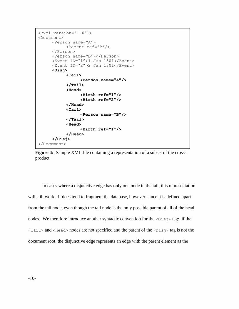
which is the full cross product. When we want only a proper subset of the cross product,
we allow multiple <Tail>/<Head> pairs as children of the <Disj> tag, as Figure 4
shows. The disjunction in Figure 4 should be interpreted in the following way: either (1)
Person A should have a child element labeled <Birth ref=“1”/>, (2) Person A should
have a child element labeled <Birth ref=“2”/>, or (3) Person B should have a child
element labeled <Birth ref=“1”/>. In other words, the cross product of each
<Tail>/<Head> pair is one of the possible interpretations.
-10-
<?xml version=“1.0”?><Document>
<Person name=“A”><Parent ref=“B”/>
</Person><Person name=“B”></Person><Event ID=“1”>1 Jan 1801</Event><Event ID=“2”>2 Jan 1801</Event><Disj>
<Tail><Person name=“A”/>
</Tail><Head>
<Birth ref=“1”/><Birth ref=“2”/>
</Head><Tail>
<Person name=“B”/></Tail><Head>
<Birth ref=“1”/></Head>
</Disj></Document>
Figure 4: Sample XML file containing a representation of a subset of the cross-product
In cases where a disjunctive edge has only one node in the tail, this representation
will still work. It does tend to fragment the database, however, since it is defined apart
from the tail node, even though the tail node is the only possible parent of all of the head
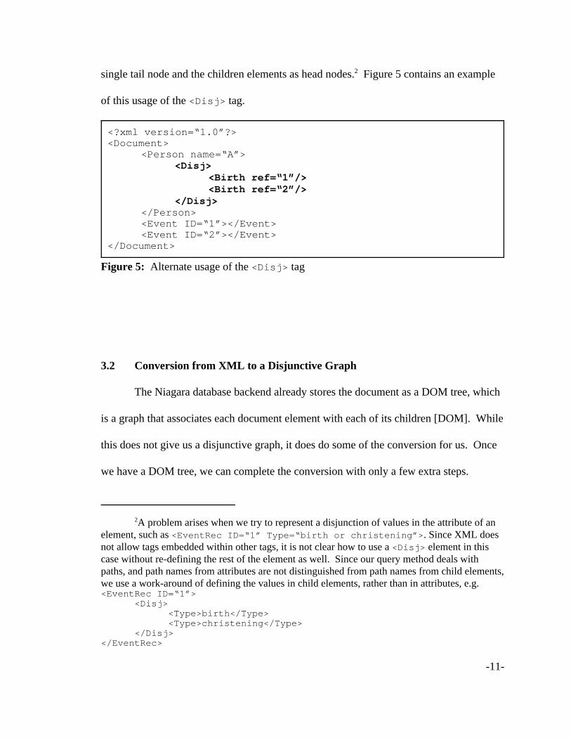
nodes. We therefore introduce another syntactic convention for the <Disj> tag: if the
<Tail> and <Head> nodes are not specified and the parent of the <Disj> tag is not the
document root, the disjunctive edge represents an edge with the parent element as the
2A problem arises when we try to represent a disjunction of values in the attribute of anelement, such as <EventRec ID=“1” Type=“birth or christening”>. Since XML doesnot allow tags embedded within other tags, it is not clear how to use a <Disj> element in thiscase without re-defining the rest of the element as well. Since our query method deals withpaths, and path names from attributes are not distinguished from path names from child elements,we use a work-around of defining the values in child elements, rather than in attributes, e.g.<EventRec ID=“1”>
<Disj><Type>birth</Type><Type>christening</Type>
</Disj></EventRec>
-11-
<?xml version=“1.0”?><Document>
<Person name=“A”><Disj>
<Birth ref=“1”/><Birth ref=“2”/>
</Disj></Person><Event ID=“1”></Event><Event ID=“2”></Event>
</Document>
Figure 5: Alternate usage of the <Disj> tag
single tail node and the children elements as head nodes.2 Figure 5 contains an example
of this usage of the <Disj> tag.
3.2 Conversion from XML to a Disjunctive Graph
The Niagara database backend already stores the document as a DOM tree, which
is a graph that associates each document element with each of its children [DOM]. While
this does not give us a disjunctive graph, it does do some of the conversion for us. Once
we have a DOM tree, we can complete the conversion with only a few extra steps.
-12-
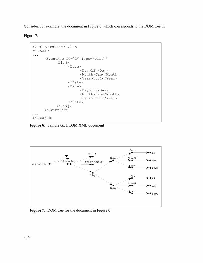
<?xml version=“1.0”?><GEDCOM>...
<EventRec Id=“1” Type=“birth”><Disj>
<Date><Day>12</Day><Month>Jan</Month><Year>1801</Year>
</Date><Date>
<Day>13</Day><Month>Jan</Month><Year>1801</Year>
</Date></Disj>
</EventRec>...</GEDCOM>
Figure 6: Sample GEDCOM XML document
G ED C O M
Id= “ 1 ”
D isj
T y p e = “ b ir th ”M o n t h
Y e a r
J a n
D a y
1 8 0 1
1 2
D a te
M o n t h
Y e a r
J a n
D a y
1 8 0 1
1 3
D a te
E v e n t R e c
Figure 7: DOM tree for the document in Figure 6
Consider, for example, the document in Figure 6, which corresponds to the DOM tree in
Figure 7.
-13-
GEDCOM :1EventRec:1
Id=“1”
Disj:1
Type=“birth” Month:1
Year:1Jan
Day:1
1801
12Date:1
Month:2
Year:2Jan
Day:2
1801
13
Date:2
Figure 8: Graph from Figure 7 after transforming node names
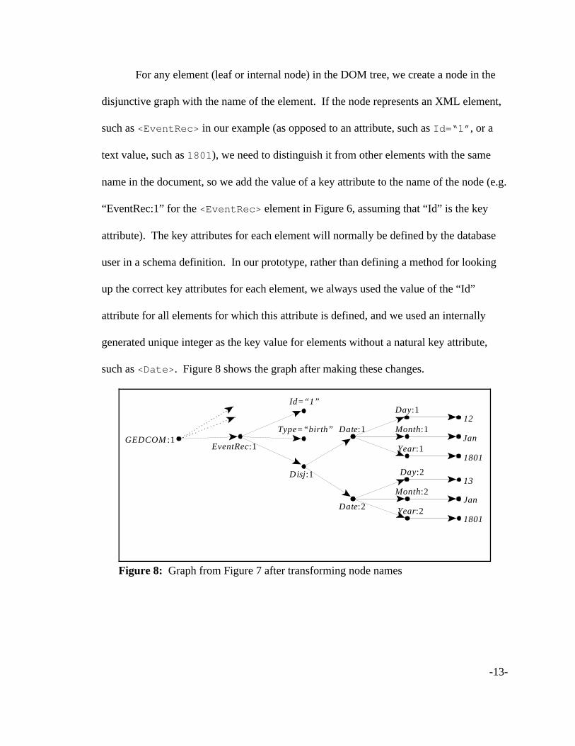
For any element (leaf or internal node) in the DOM tree, we create a node in the
disjunctive graph with the name of the element. If the node represents an XML element,
such as <EventRec> in our example (as opposed to an attribute, such as Id=“1”, or a
text value, such as 1801), we need to distinguish it from other elements with the same
name in the document, so we add the value of a key attribute to the name of the node (e.g.
“EventRec:1” for the <EventRec> element in Figure 6, assuming that “Id” is the key
attribute). The key attributes for each element will normally be defined by the database
user in a schema definition. In our prototype, rather than defining a method for looking
up the correct key attributes for each element, we always used the value of the “Id”
attribute for all elements for which this attribute is defined, and we used an internally
generated unique integer as the key value for elements without a natural key attribute,
such as <Date>. Figure 8 shows the graph after making these changes.
3Note that since this creates aliasing among several records, updates to the databaseshould change the edges in the graph, rather than the values of the nodes. Note also that careshould be taken if the value of any node could be equal to the internal representation of anelement concatenated with its key attribute (e.g. “EventRec:1”).
-14-
GEDCOM :1
1
D isj:1
birthEventRec:1Month :1
Year:1
Jan
Day :1
1801
12
Date:1
Month :2
Year:2
Day :213
Date:2
EventRec Type
Id
Date
Date
Day
DayMonth
Month
Year
Year
text
text
text
text
text
text
Figure 9: Graph from Figure 8 after adding edge names
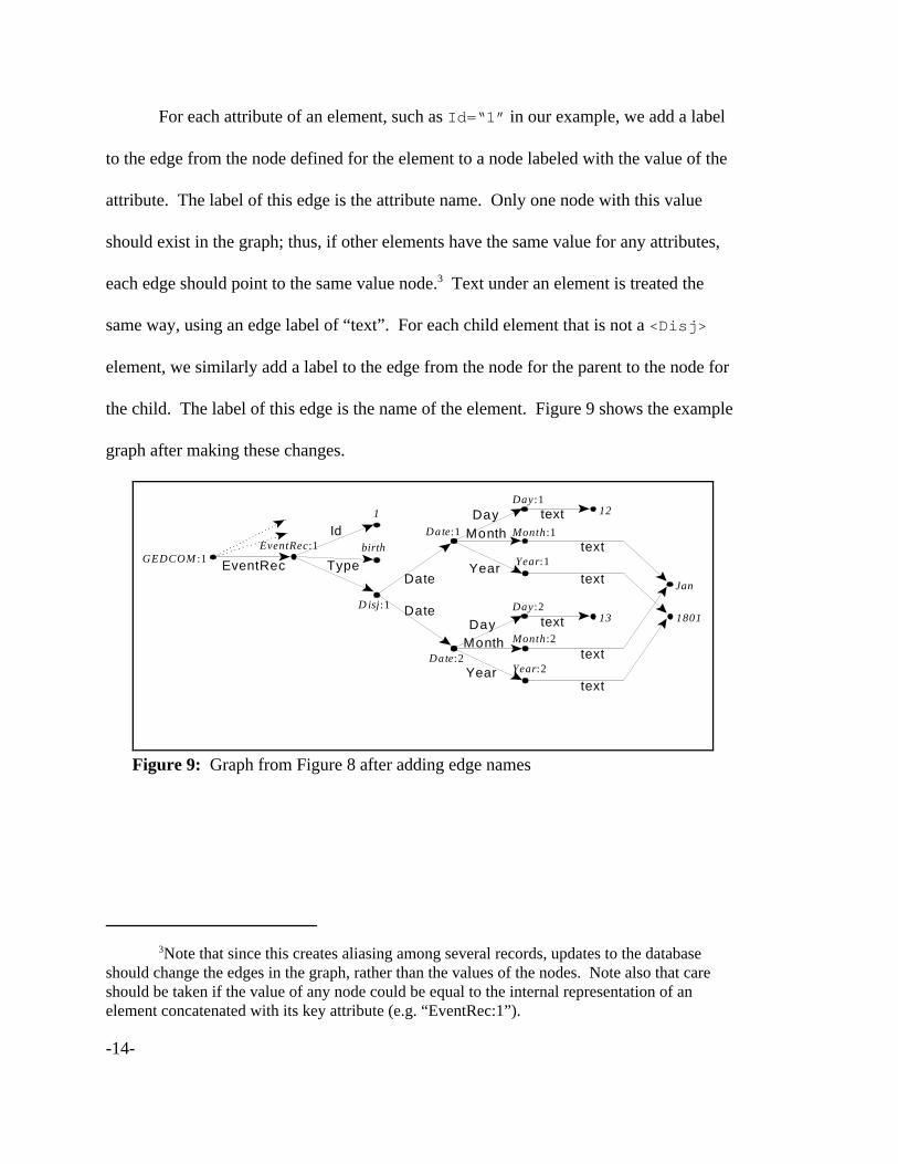
For each attribute of an element, such as Id=“1” in our example, we add a label
to the edge from the node defined for the element to a node labeled with the value of the
attribute. The label of this edge is the attribute name. Only one node with this value
should exist in the graph; thus, if other elements have the same value for any attributes,
each edge should point to the same value node.3 Text under an element is treated the
same way, using an edge label of “text”. For each child element that is not a <Disj>
element, we similarly add a label to the edge from the node for the parent to the node for
the child. The label of this edge is the name of the element. Figure 9 shows the example
graph after making these changes.

-15-
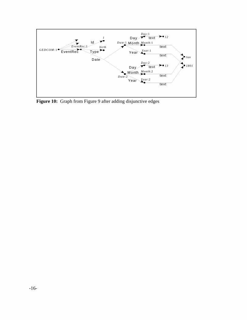
For each child element labeled <Disj>, since we have defined two possible
contexts for a disjunction, we have to check which type of disjunction it is. If the
children of the <Disj> element are <Tail>/<Head> pairs, we construct a separate
disjunctive edge with the set of child elements of <Tail> and of <Head> as the tail and
head, respectively. Note that the child elements must be defined with their key attributes
in order to attach the edge to the correct nodes in the graph. We have to treat the case
where we have multiple <Tail>/<Head> pairs special, since a single edge can only
represent the full cross product of the tail and the head. In our implementation, we store
this type of disjunction separately from the rest of the graph as a set of edges.
The other context for a disjunction is when the children of the <Disj> element
are not <Tail> and <Head> elements, but are implicitly only head elements. In this
case, we replace the <Disj> node and its incident edges with a single disjunctive edge
from the parent of the <Disj> element to the set of its child elements. If all of the child
elements have the same name, the name of this disjunctive edge is the name of its
elements. Otherwise, there is no single name that correctly represents this edge. In our
implementation, we assign the name to the empty string.
Figure 10 shows the final disjunctive graph of the example data from Figure 6.
Since we can complete this conversion with one pass of the entire XML document, the
entire conversion requires only O(m + n + p) time, where m is the number of edges in the
document, n is the number of nodes, and p is the number of values.
-16-
GEDCOM :1EventRec :1
Month :1
Year:1
Jan
Day :1
1801
12
D a te:1
Month :2
Year:2
Day :213
D a te:2
EventRec Type
Id
Date
Day
DayMonth
Month
Year
Year
text
text
text
text
text
text
1
birth
Figure 10: Graph from Figure 9 after adding disjunctive edges
-17-
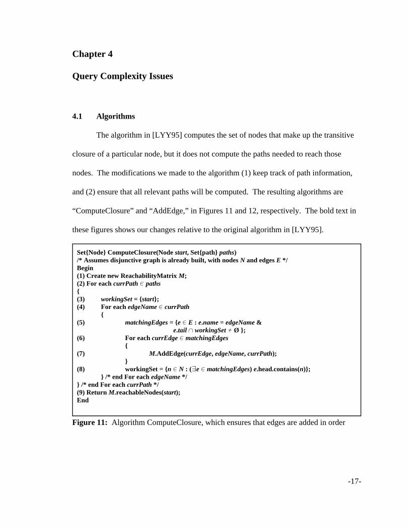
Set{Node} ComputeClosure(Node start, Set{path} paths)/* Assumes disjunctive graph is already built, with nodes N and edges E */Begin(1) Create new ReachabilityMatrix M;(2) For each currPath 0 paths{(3) workingSet = {start};(4) For each edgeName 0 currPath
{(5) matchingEdges = {e 0 E : e.name = edgeName &
e.tail 1 workingSet … Ø };(6) For each currEdge 0 matchingEdges
{(7) M.AddEdge(currEdge, edgeName, currPath);
}(8) workingSet = {n 0 N : (›e 0 matchingEdges) e.head.contains(n)};
} /* end For each edgeName */} /* end For each currPath */(9) Return M.reachableNodes(start);End
Figure 11: Algorithm ComputeClosure, which ensures that edges are added in order
Chapter 4
Query Complexity Issues
4.1 Algorithms
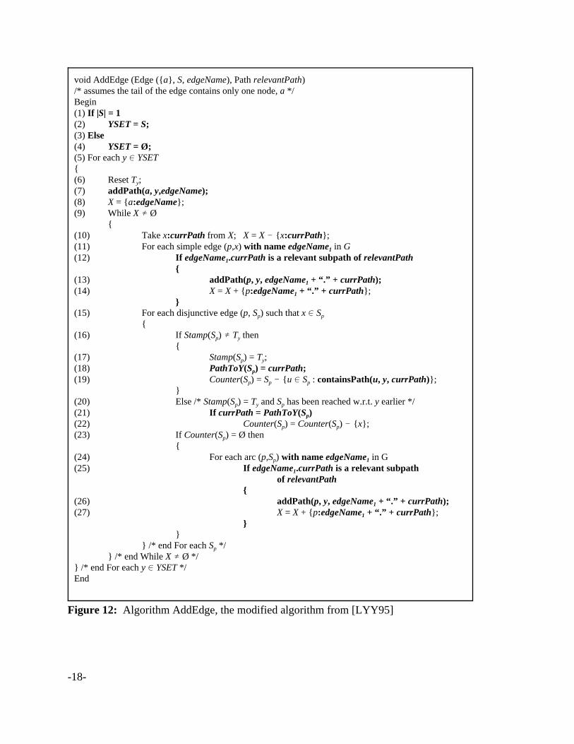
The algorithm in [LYY95] computes the set of nodes that make up the transitive
closure of a particular node, but it does not compute the paths needed to reach those
nodes. The modifications we made to the algorithm (1) keep track of path information,
and (2) ensure that all relevant paths will be computed. The resulting algorithms are
“ComputeClosure” and “AddEdge,” in Figures 11 and 12, respectively. The bold text in
these figures shows our changes relative to the original algorithm in [LYY95].
-18-
void AddEdge (Edge ({a}, S, edgeName), Path relevantPath)/* assumes the tail of the edge contains only one node, a */Begin(1) If |S| = 1(2) YSET = S;(3) Else(4) YSET = Ø;(5) For each y 0 YSET{(6) Reset Ty;(7) addPath(a, y,edgeName);(8) X = {a:edgeName};(9) While X … Ø
{(10) Take x:currPath from X; X = X ! {x:currPath};(11) For each simple edge (p,x) with name edgeName1 in G(12) If edgeName1.currPath is a relevant subpath of relevantPath
{(13) addPath(p, y, edgeName1 + “.” + currPath);(14) X = X + {p:edgeName1 + “.” + currPath};
}(15) For each disjunctive edge (p, Sp) such that x 0 Sp
{(16) If Stamp(Sp) … Ty then
{(17) Stamp(Sp) = Ty;(18) PathToY(Sp) = currPath;(19) Counter(Sp) = Sp ! {u 0 Sp : containsPath(u, y, currPath)};
}(20) Else /* Stamp(Sp) = Ty and Sp has been reached w.r.t. y earlier */(21) If currPath = PathToY(Sp)(22) Counter(Sp) = Counter(Sp) ! {x};(23) If Counter(Sp) = Ø then
{(24) For each arc (p,Sp) with name edgeName1 in G(25) If edgeName1.currPath is a relevant subpath
of relevantPath{
(26) addPath(p, y, edgeName1 + “.” + currPath);(27) X = X + {p:edgeName1 + “.” + currPath};
}}
} /* end For each Sp */} /* end While X … Ø */
} /* end For each y 0 YSET */End
Figure 12: Algorithm AddEdge, the modified algorithm from [LYY95]

-19-
4.2 Foundations for a Polynomial-Time Solution
To help explain the modifications, we first introduce some formal definitions. We
then establish the need for a polynomial-time solution by showing that the number of
possible paths is exponential.
Definition 1: A node is any string value designated as representing a database value.
Definition 2: An edge is an ordered triple (T, H, n) where T and H are non-empty sets of
nodes and n is a string. We call T the tail of the edge, H the head of the edge, and n the
name of the edge. We say that T is a disjunctive tail if |T| > 1. Similarly, we say that H is
a disjunctive head if |H| > 1. The edge is a disjunctive edge if either the head or the tail is
disjunctive, otherwise it is a simple edge. For example, ({Day:1}, {12}, text) is a simple
edge in Figure 10, and ({EventRec:1}, {Date:1, Date:2}, Date) is a disjunctive edge.
Definition 3: A graph is an ordered pair (N, E) where N is a set of nodes and E is a set of
edges such that for each (T, H, n) 0 E, T f N and H f N.
Definition 4: A path between two nodes x and y in a graph (N, E) is a sequence (p1, p2,
..., pk) of strings such that:
1. If the length of the sequence is 1, then there exists an edge (T, H, p1) in E such that
x 0 T and y 0 H.
2. If the length of the sequence is greater than 1, then for some z 0 N, there exists an
edge (T, H, p1) in E such that x 0 T and z 0 H and there exists a path (p2,..., pk)
from z to y.
-20-
An equivalent representation of a path (p1, p2, ..., pk) is p1.p2.AAA.pk. The length of a path
p1.p2.AAA.pk is k, the length of the sequence. We can also represent the length of a path
p1.p2.AAA.pk by |p1.p2.AAA.pk|. For example, in the graph in Figure 10, “Month.text” is a path
from node Date:1 to node Jan; it is also a path from Date:2 to Jan.
Definition 5: An edge (T, H, n) matches a path p at position i for 1 # i # k if n = pi,
where p = p1.p2.AAA.pk. We can equivalently say that the name of the edge n matches p at
position i. For example, the edge ({Month:1}, {Jan}, text) matches the path
“Month.text” at position 2.
Definition 6: A subpath of a path p1.p2.AAA.pk is a sequence pi.pi+1.AAA.pi+j where 1 # i # i +
j # k. The suffix of a path p1.p2.AAA.pk for k $ 2 is the subpath p2.AAA.pk. Note that the suffix
is not defined for a path with length less than 2. For example, “Date.Month” is a subpath
of “EventRec.Date.Month.text”. “Date.Month.text” is a subpath which is also the suffix
of “EventRec.Date.Month.text”.
Definition 7: A node y is reachable through path p from node x in graph G if every
interpretation of G contains the path p from x to y. In Figure 10, for example, the node
Jan is reachable from EventRec:1 through the path “Date.Month.text”, but node Date:1 is
not reachable from EventRec:1 through the path “Date”.
Definition 8: A node of interest to a path p and a node x is a node y that is always
reachable from x through a subpath of p.
The solution we present is based on two observations: (1) We need to guarantee
that a node is always reachable by a certain path in every possible interpretation. (2) We
must limit the number of paths we store and work with in the algorithm, because the
-21-
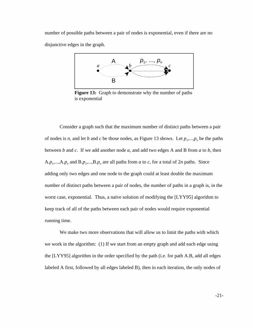
b cp1, ..., pn
a
B
A
Figure 13: Graph to demonstrate why the number of pathsis exponential
number of possible paths between a pair of nodes is exponential, even if there are no
disjunctive edges in the graph.
Consider a graph such that the maximum number of distinct paths between a pair
of nodes is n, and let b and c be those nodes, as Figure 13 shows. Let p1,...,pn be the paths
between b and c. If we add another node a, and add two edges A and B from a to b, then
A.p1,...,A.pn and B.p1,...,B.pn are all paths from a to c, for a total of 2n paths. Since
adding only two edges and one node to the graph could at least double the maximum
number of distinct paths between a pair of nodes, the number of paths in a graph is, in the
worst case, exponential. Thus, a naïve solution of modifying the [LYY95] algorithm to
keep track of all of the paths between each pair of nodes would require exponential
running time.
We make two more observations that will allow us to limit the paths with which
we work in the algorithm: (1) If we start from an empty graph and add each edge using
the [LYY95] algorithm in the order specified by the path (i.e. for path A.B, add all edges
labeled A first, followed by all edges labeled B), then in each iteration, the only nodes of
-22-
interest will be in the head of the added edge. (2) In each iteration, we will only find
potential nodes of interest if the edge in the current iteration is a simple edge.
To understand the first observation, consider path A.B as an example. First we
determine all the nodes of interest through the subpath A. If in a given iteration we add
an edge labeled A, any path to newly discovered nodes of interest must go through this
edge. If there are any other nodes of interest besides the node(s) in the head of the edge,
then they must be reachable through another edge already added. Since the only edges
that could be added before this edge are other edges labeled A, the new path to these
nodes must begin with A.A, and thus these nodes are not of interest.
After finding these nodes of interest, we next determine all the nodes of interest
through the subpath A.B. During an iteration that adds an edge labeled B, any path to
newly discovered nodes of interest must go through this edge. Any nodes other than the
node(s) in the head of this edge must also go through other edges after the new B edge.
Paths to these nodes must therefore contain edges after the B, and therefore they are not
of interest.
To understand the second observation, suppose that on any iteration we add a
disjunctive edge. Lemma 2 in [LYY95] states that any nodes that become reachable after
adding such an edge must also be reachable from each node in the head of this edge.
Since nodes of interest must be reachable as part of the definition, any newly discovered
nodes of interest must also be reachable through all the nodes in the head of this edge.
Similar to the first observation, any path to these nodes must go through other edges after
the newly added edge, and therefore cannot be nodes of interest. This even includes the

-23-
nodes in the head, since they must also be reachable through the other nodes in the head.
Thus, adding a disjunctive edge will not result in adding new nodes of interest.
4.3 Path-connections and Reachability
We now introduce the concept of a path-connection, and prove that, under certain
conditions, finding all path-connections is equivalent to finding the set of all reachable
nodes.
Definition 9: a path-connection through path p from node x to node y in a disjunctive
graph (N, E) is defined as a tuple (x, S, y, p) where x, y 0 N and S f N and either:
1. |p| = 1, S = {y}, and there exists an edge ({x}, S, p) (i.e. a simple edge from
x to y) in E; or
2. |p| > 1 (in which case, let p1 be the first edge of p and ps be the suffix of p),
for each u 0 S there is a path-connection through ps from u to y, and there
exists an edge ({x}, S, p1) in E.
Example: In Figure 10, (Month:1, {Jan}, Jan, text) is a path-connection through
the path “text” from Month:1 to Jan, since there is an edge ({Month:1}, {Jan}, text) in
the graph, thus satisfying case 1. (Date:1, {Month:1}, Jan, Month.text) is a path-
connection through the path “Month.text” from Date:1 to Jan, since there is a path-
connection through “text” from Month:1 to Jan, and there is an edge ({Date:1},
{Month:1}, Month) in the graph, thus satisfying case 2. Likewise, (EventRec:1, {Date:1,
Date:2}, Jan, Date.Month.text) is a path-connection through the path “Date.Month.text”
-24-
from EventRec:1 to Jan, since both Date:1 and Date:2 have path-connections through
“Month.text” to Jan and the edge ({EventRec:1}, {Date:1, Date:2}, Date) exists.
Theorem 1: Let G = (N, E) be a graph such that no edge in E has a disjunctive tail, and
let p be a path such that no disjunctive edge in E matches p at more than one position.
For any nodes x and y in G, there is a path-connection through p from x to y if and only if
y is reachable from x through path p in every interpretation of G.
Proof: The proof is similar to the proof for Lemma 1 in [LYY95].
(The ONLY IF part will be proved by induction on the length of path p.)
Basis: If the length of p is 1, then the path-connection from x to y must satisfy
case 1; that is, S = {y} and there exists an edge ({x}, {y}, p) in G. Since this is not a
disjunctive edge, it must appear in every interpretation of G, and thus y is reachable from
x through this edge in every interpretation.
Induction: Assume the length of p is greater than 1. Thus the path-connection
from x to y must satisfy case 2; that is, for each u 0 S there is a path-connection through
ps from u to y, and there exists an edge ({x}, S, p1) in G, where p1 is the first edge of p and
ps is the suffix of p. Since p = p1.ps, |ps| = |p| ! 1. Thus, by our inductive hypothesis, for
each u 0 S, y is reachable from u through ps in every interpretation of G. Given any
interpretation of G, we know that the interpretation must contain an edge ({x}, {u}, p1)
for some u 0 S. (If |S| = 1, then ({x}, S, p1) represents a simple edge, and it must appear
in any interpretation of G. The argument remains the same.) Since we already know that
-25-
any interpretation must contain a path from u to y labeled ps, we can concatenate the paths
p1 and ps to get a path from x to y labeled p1.ps = p.
(For the IF part, we prove by contradiction that if there is no path-connection
through p from x to y, then there exists an interpretation I in which y is not reachable from
x through path p.)
Given graph G, construct an interpretation I as follows: for each simple edge
({u}, {v}, n) in G, add a corresponding edge ({u}, {v}, n) to I. For each disjunctive edge
({u}, S, q1) in G, by the hypothesis there is at most one position in p that q1 can match. If
q1 does not match at any position in p then replace ({u}, S, q1) with ({u}, {v}, q1) for any
v 0 S. Otherwise, let q be the sub-path of p that begins at q1 and ends at the last edge of
p. If there is a path connection through q from u to y, then replace ({u}, S, q1) with ({u},
{v}, q1) for any v 0 S. Otherwise, there is no path connection through q from u to y, so by
definition, we have two possibilities:
1. |q| = 1, and thus q = q1. Then either S … {y} or the edge ({u}, S, q1) does
not exist. Since we know this edge exists, we are left with S … {y}. Since
an edge cannot have an empty tail, S must contain some element v … y.
Replace ({u}, S, q1) with ({u}, {v}, q1) in I.
2. |q| > 1, and thus q = q1.qs where qs is the suffix of q. Then either there
exists some v 0 S such that there is no path-connection through qs from v
to y, or the edge ({u}, S, q1) does not exist. Since we know this edge
exists, there must exist some such v 0 S. Replace ({u}, S, q1) with ({u},
{v}, q1) in I.
-26-
Since we have replaced each edge in G with an edge in I, I is a valid interpretation
of G. Now, assume that y is reachable from x through path p in I. Let z be the last node
on the path before y, and let q be the edge name. Then there must be a path-connection
through q from z to y in G, because either ({z}, {y}, q) was created from a simple edge
({z}, {y}, q) in G, in which case ({z}, {y}, q) exists in any interpretation of G, or it was
created from a disjunctive edge ({z}, S, q), and since |q| = 1, (from case 1, above), if there
were not a path-connection through q, this disjunctive edge in G would have been
replaced by edge ({z}, {v}, q) for some v … y.
Since there is at least one node in the path (namely, z) that has a path-connection
to y through a subpath of p, and at least one node in the path (namely, x) that does not,
there must be two consecutive nodes u and v on the path such that there is a path-
connection from v to y through a subpath of p in G (let qs be this subpath), but no such
path-connection from u to y. Let ({u}, {v}, q1) be the edge connecting u to v along path p
in I. Since u and v are consecutive nodes, q1.qs is also a subpath of p. If this edge had
been generated from a simple edge ({u}, {v}, q1) in G, then since there is a path-
connection through qs from v to y, by definition there is a path-connection through q1.qs
from u to y, contradicting our assumption. Thus, the edge must have been generated from
a disjunctive edge ({u}, S, q1) with v 0 S. We have already established that there is no
path-connection from u to y through q1.qs, and since |qs| > 0, |q1.qs| > 1, so case 2 applies.
But that means that since ({u}, S, q1) was replaced by edge ({u}, {v}, q1), there must not
be a path-connection through qs from v to y, contradicting our assumption that there is a
path-connection through qs from v to y. Therefore, there must be no such path p in I. #
-27-
a
b
c
d
e f
gA
A B
B
C
B
C
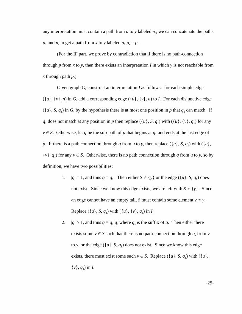
Figure 14: Graph that does not satisfy the conditions of Theorem 1
It is important to explain why we must include the condition that no disjunctive
edge in G can match at more than one position in the path. The graph in Figure 14 has
only one disjunctive edge, and therefore only two valid interpretations. It is easy to verify
that node g is reachable from node a through path A.B.B.C in both interpretations;
however, there is not a path-connection through A.B.B.C from a to g in the original
graph. This is because our definition of path-connection would require a path-connection
through either B.B.C or B.C from c to g, which would in turn require path-connections
from d to g and from e to g through either B.C or C, respectively. While each
interpretation does contain one of these two paths, neither path alone appears in both
interpretations.
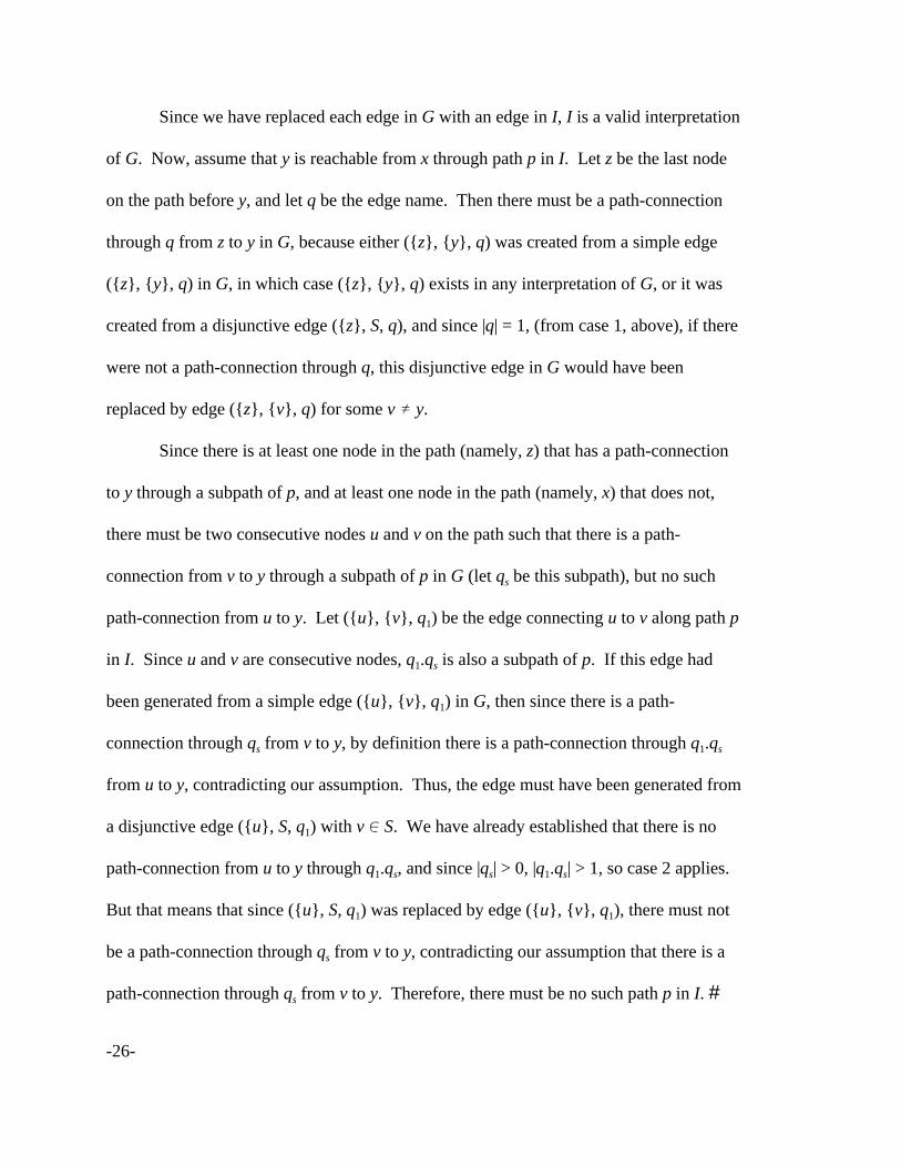
-28-
a
b
c e
A
A
dA
f
B
B
Figure 15: Graph that does not satisfy the conditions of Theorem 1, butwould still work with the modified algorithm
It is also important to note that while the absence of such disjunctive edges is a
sufficient condition for the algorithm to work, it is not a necessary condition. The
disjunctive edge in the graph in Figure 15 matches at two positions in the path A.A.B;
however, we can say that there is a path-connection from a to f through A.A.B, since both
b and c have path-connections to f through A.B. The difference lies in the fact that while
the disjunctive edge could match both the first and the second A in the path, it only
participates in the first. We leave the development of a stronger condition for graphs that
will work with the modified algorithm as future work.
4.4 Simulation of the New Algorithm
We demonstrate the execution of the modified algorithm by simulating it on the
disjunctive graph in Figure 16, using the query “find all values reachable by path
A.B.C.D.E from node a.” It is easy to see that node h is always reachable, but not so easy
to see that it belongs in the answer to this query. This graph is somewhat complicated,
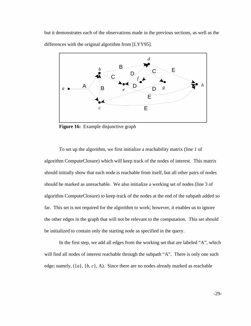
-29-
a
b
c
d
e
f
gA
B
Bh
CCD
D D
E
E
E
Figure 16: Example disjunctive graph
but it demonstrates each of the observations made in the previous sections, as well as the
differences with the original algorithm from [LYY95].
To set up the algorithm, we first initialize a reachability matrix (line 1 of
algorithm ComputeClosure) which will keep track of the nodes of interest. This matrix
should initially show that each node is reachable from itself, but all other pairs of nodes
should be marked as unreachable. We also initialize a working set of nodes (line 3 of
algorithm ComputeClosure) to keep track of the nodes at the end of the subpath added so
far. This set is not required for the algorithm to work; however, it enables us to ignore
the other edges in the graph that will not be relevant to the computation. This set should
be initialized to contain only the starting node as specified in the query.
In the first step, we add all edges from the working set that are labeled “A”, which
will find all nodes of interest reachable through the subpath “A”. There is only one such
edge; namely, ({a}, {b, c}, A). Since there are no nodes already marked as reachable
-30-
from all nodes in the head of this edge (i.e. nodes b and c), this does not change the
reachability matrix. The working set now gets changed to {b, c}.
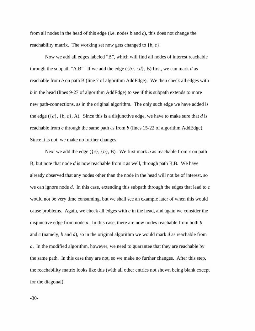
Now we add all edges labeled “B”, which will find all nodes of interest reachable
through the subpath “A.B”. If we add the edge ({b}, {d}, B) first, we can mark d as
reachable from b on path B (line 7 of algorithm AddEdge). We then check all edges with
b in the head (lines 9-27 of algorithm AddEdge) to see if this subpath extends to more
new path-connections, as in the original algorithm. The only such edge we have added is
the edge ({a}, {b, c}, A). Since this is a disjunctive edge, we have to make sure that d is
reachable from c through the same path as from b (lines 15-22 of algorithm AddEdge).
Since it is not, we make no further changes.
Next we add the edge ({c}, {b}, B). We first mark b as reachable from c on path
B, but note that node d is now reachable from c as well, through path B.B. We have
already observed that any nodes other than the node in the head will not be of interest, so
we can ignore node d. In this case, extending this subpath through the edges that lead to c
would not be very time consuming, but we shall see an example later of when this would
cause problems. Again, we check all edges with c in the head, and again we consider the
disjunctive edge from node a. In this case, there are now nodes reachable from both b
and c (namely, b and d), so in the original algorithm we would mark d as reachable from
a. In the modified algorithm, however, we need to guarantee that they are reachable by
the same path. In this case they are not, so we make no further changes. After this step,
the reachability matrix looks like this (with all other entries not shown being blank except
for the diagonal):
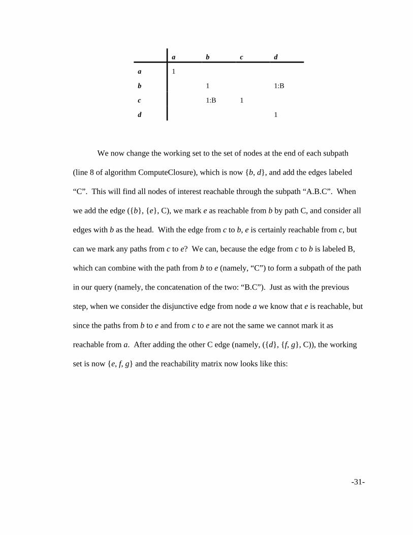
-31-
a b c d
a 1
b 1 1:B
c 1:B 1
d 1
We now change the working set to the set of nodes at the end of each subpath
(line 8 of algorithm ComputeClosure), which is now {b, d}, and add the edges labeled
“C”. This will find all nodes of interest reachable through the subpath “A.B.C”. When
we add the edge ({b}, {e}, C), we mark e as reachable from b by path C, and consider all
edges with b as the head. With the edge from c to b, e is certainly reachable from c, but
can we mark any paths from c to e? We can, because the edge from c to b is labeled B,
which can combine with the path from b to e (namely, “C”) to form a subpath of the path
in our query (namely, the concatenation of the two: “B.C”). Just as with the previous
step, when we consider the disjunctive edge from node a we know that e is reachable, but
since the paths from b to e and from c to e are not the same we cannot mark it as
reachable from a. After adding the other C edge (namely, ({d}, {f, g}, C)), the working
set is now {e, f, g} and the reachability matrix now looks like this:
-32-
a b c d e
a 1
b 1 1:B 1:C
c 1:B 1 1:B.C
d 1
e 1
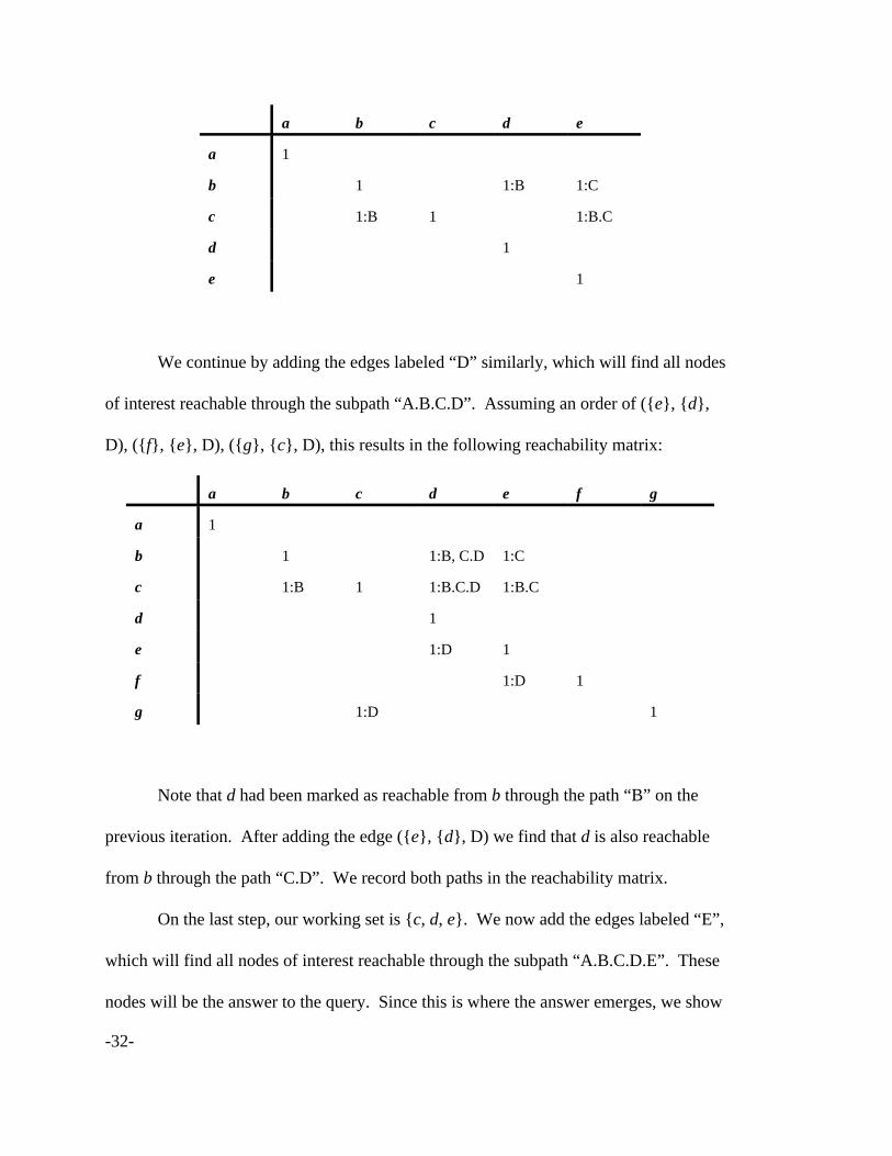
We continue by adding the edges labeled “D” similarly, which will find all nodes
of interest reachable through the subpath “A.B.C.D”. Assuming an order of ({e}, {d},
D), ({f}, {e}, D), ({g}, {c}, D), this results in the following reachability matrix:
a b c d e f g
a 1
b 1 1:B, C.D 1:C
c 1:B 1 1:B.C.D 1:B.C
d 1
e 1:D 1
f 1:D 1
g 1:D 1
Note that d had been marked as reachable from b through the path “B” on the
previous iteration. After adding the edge ({e}, {d}, D) we find that d is also reachable
from b through the path “C.D”. We record both paths in the reachability matrix.
On the last step, our working set is {c, d, e}. We now add the edges labeled “E”,
which will find all nodes of interest reachable through the subpath “A.B.C.D.E”. These
nodes will be the answer to the query. Since this is where the answer emerges, we show
-33-
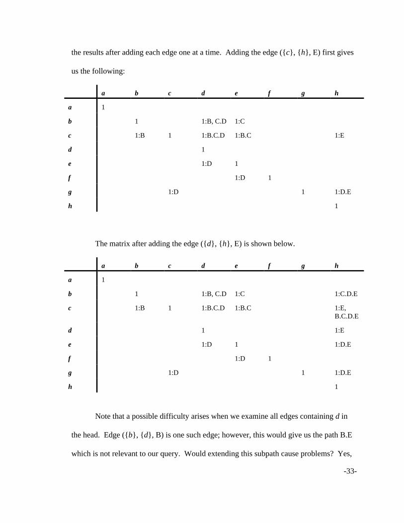
the results after adding each edge one at a time. Adding the edge ({c}, {h}, E) first gives
us the following:
a b c d e f g h
a 1
b 1 1:B, C.D 1:C
c 1:B 1 1:B.C.D 1:B.C 1:E
d 1
e 1:D 1
f 1:D 1
g 1:D 1 1:D.E
h 1
The matrix after adding the edge ({d}, {h}, E) is shown below.
a b c d e f g h
a 1
b 1 1:B, C.D 1:C 1:C.D.E
c 1:B 1 1:B.C.D 1:B.C 1:E,B.C.D.E
d 1 1:E
e 1:D 1 1:D.E
f 1:D 1
g 1:D 1 1:D.E
h 1
Note that a possible difficulty arises when we examine all edges containing d in
the head. Edge ({b}, {d}, B) is one such edge; however, this would give us the path B.E
which is not relevant to our query. Would extending this subpath cause problems? Yes,
4 Note that this may cause us to “add” an edge more than once if it matches at more thanone position in the path, in order to extend new subpaths at different positions. Since we onlyadd an edge at most once at each position of the path, however, this is still limited by the lengthof the path.
-34-
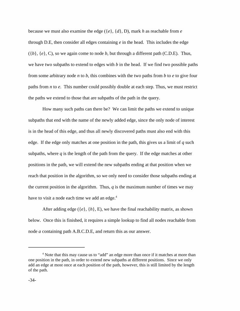
because we must also examine the edge ({e}, {d}, D), mark h as reachable from e
through D.E, then consider all edges containing e in the head. This includes the edge
({b}, {e}, C), so we again come to node b, but through a different path (C.D.E). Thus,
we have two subpaths to extend to edges with b in the head. If we find two possible paths
from some arbitrary node n to b, this combines with the two paths from b to e to give four
paths from n to e. This number could possibly double at each step. Thus, we must restrict
the paths we extend to those that are subpaths of the path in the query.
How many such paths can there be? We can limit the paths we extend to unique
subpaths that end with the name of the newly added edge, since the only node of interest
is in the head of this edge, and thus all newly discovered paths must also end with this
edge. If the edge only matches at one position in the path, this gives us a limit of q such
subpaths, where q is the length of the path from the query. If the edge matches at other
positions in the path, we will extend the new subpaths ending at that position when we
reach that position in the algorithm, so we only need to consider those subpaths ending at
the current position in the algorithm. Thus, q is the maximum number of times we may
have to visit a node each time we add an edge.4
After adding edge ({e}, {h}, E), we have the final reachability matrix, as shown
below. Once this is finished, it requires a simple lookup to find all nodes reachable from
node a containing path A.B.C.D.E, and return this as our answer.
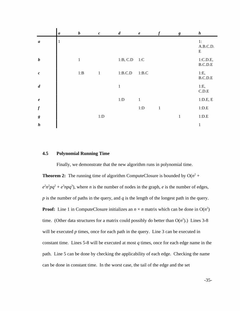
-35-
a b c d e f g h
a 1 1:A.B.C.D.E
b 1 1:B, C.D 1:C 1:C.D.E,B.C.D.E
c 1:B 1 1:B.C.D 1:B.C 1:E,B.C.D.E
d 1 1:E,C.D.E
e 1:D 1 1:D.E, E
f 1:D 1 1:D.E
g 1:D 1 1:D.E
h 1
4.5 Polynomial Running Time
Finally, we demonstrate that the new algorithm runs in polynomial time.
Theorem 2: The running time of algorithm ComputeClosure is bounded by O(n2 +
e2n2pq2 + e3npq3), where n is the number of nodes in the graph, e is the number of edges,
p is the number of paths in the query, and q is the length of the longest path in the query.
Proof: Line 1 in ComputeClosure initializes an n × n matrix which can be done in O(n2)
time. (Other data structures for a matrix could possibly do better than O(n2).) Lines 3-8
will be executed p times, once for each path in the query. Line 3 can be executed in
constant time. Lines 5-8 will be executed at most q times, once for each edge name in the
path. Line 5 can be done by checking the applicability of each edge. Checking the name
can be done in constant time. In the worst case, the tail of the edge and the set
-36-
workingSet could contain as many as n nodes, so calculating the intersection could
require O(n) time. Since this is done for each edge, line 5 requires at most O(en) time.
Line 7 is executed at most e times. Line 8 could require us, in the worst case, to check all
the edges. Since this is done for all the nodes, this would require O(en) time. Line 9
requires us to traverse one line of the reachability matrix, which requires only O(n) time.
The total running time is O(n2 + p @ q @ (en + e @ T) + n) = O(n2 + pq(en + e @ T)) where T
is the running time of algorithm AddEdge.
We now calculate the running time of algorithm AddEdge. Lines 1-4 require only
constant time, because if |S| > 1, we only have to initialize YSET to the empty set. The
loop from lines 5-27 will be executed at most once, since the size of YSET is at most 1.
Lines 6-8 can be done in constant time, assuming that line 7 can add the path to a hash
table with a good hash function. The while loop in lines 9-27 will be executed at most nq
times, since each node will be examined once for each position in the path, as already
discussed. Line 10 requires us to load the path from node x to node y, which could be as
long as q.
The loop from lines 11-14 will be executed at most e times. The condition in line
12 may require us to check each position in the path, which is at most q. Lines 13-14
require us to store a new path from p to y, which could also be as long as q. Thus, lines
11-14 can be executed in O(eq) time.
The loop from lines 15-27 will be executed at most e times. Lines 16 and 17 can
be done in constant time. Line 18 requires us to store the current path from x to y, which
could be as long as q. Line 19 requires us to check each node in the head of the edge,
-37-
which could be as many as n checks. It also requires us to look up the current path, which
could be as long as q, so the total time required for line 19 is O(nq). Similarly, lines 20-
22 will require us to store the current path, which requires O(q) time. Thus, lines 16-22
can be executed in O(nq) time.
The loop in Lines 24-27 will be executed at most e times. Lines 25-27 require us
to look up and store paths which are bounded by q. Thus, lines 24-27 can be executed in
O(eq) time.
Putting the code from lines 15-27 together thus requires O(e @ (nq + eq)) = O(enq
+ e2q) time. Adding this to the rest of the loop from lines 9-27 requires O(nq @ (eq + enq
+ e2q)) = O(en2q2 + e2nq2) time. Thus, the entire AddEdge algorithm requires O(q + en2q2
+ e2nq2) = O(en2q2 + e2nq2) time.
Substituting this back in to the running time of algorithm ComputeClosure gives a
total worst-case running time of O(n2 + pq(en + e @ (en2q2 + e2nq2)) = O(n2 + pq(en + e2n2q
+ e3nq2)) = O(n2 + pq(e2n2q + e3nq2)) = O(n2 + e2n2pq2 + e3npq3).

-38-
-39-
Chapter 5
Analysis and Results
We programmed a prototype database to handle disjunctive data and perform
queries. The host machine for the database was a dual-processor P3 running at 850MHz,
with a 256KB cache and 512 MB of RAM, running Debian Linux (using the 2.4.20 SMP
kernel). The compiler we used was the GNU C++ Compiler (gcc) version 2.95.4. The
data was stored on a RAID-5 system with 205.1GB of storage space, using the Adaptec
I2O 3210S version 2.4 drivers.
We programmed 4 algorithms for a timing comparison. The first was a brute-
force algorithm. Given a particular query, this algorithm constructs every possible
interpretation of the graph, calculates the set of nodes that answer the query in each
interpretation, and returns the intersection of all the sets. Since this algorithm always
checks every interpretation, its running time follows an exponential curve with respect to
the number of disjunctive edges.
The second algorithm was a backtracking algorithm, which performs a depth-first
search on the graph. If it encounters a disjunctive edge, it replaces the edge with one of
the simple edges it represents, and finishes calculating the set of nodes that answer the
query (similarly replacing other disjunctive edges it encounters). It then replaces the edge
with another one of the edges it represents and again calculates the set of nodes that
answer the query, and so forth until all possible edges have been checked. It then
computes the intersection of the sets it calculated. While this algorithm avoids
-40-
calculating every possible interpretation of the graph, it may run into the same disjunctive
edges multiple times. In a highly connected graph with e edges, each step could in the
worst case lead us to examine all e ! 1 of the other edges in the next step, which could
lead to e ! 2 in the next step, and so forth. This gives us a worst-case running time of e @
(e ! 1) @ (e ! 2) @ ... = e!. Caching results could improve this running time, at the expense
of using more memory, but since most genealogy data is not highly connected, our
backtracking algorithm does not use caching.
The third algorithm executed the query using the modified [LYY95] algorithm,
which runs in polynomial time. The fourth algorithm was a heuristic that removes all
disjunctive edges from the graph and answers the query based on the remaining edges.
Since it removes the disjunctive edges, it does not give a complete answer; however, it
provides a comparison to typical query engines for databases that do not contain
disjunctive data.
The chart in Figure 17 compares the running times of each algorithm for a simple
query on a small genealogy database containing data for three generations of people and
varying numbers of disjunctive edges. The query returns all known information about an
individual, without any path information. Because both axes of the graph have a
logarithmic scale, a straight line indicates a polynomial-time algorithm, while a curved
line shows an exponential algorithm. The graph shows two interesting conclusions.
First, for the test with only two disjunctive arcs, both the brute-force and the backtracking
algorithms out-perform the polynomial-time algorithm. With such a small number of
disjunctions, the polynomial-time algorithm has enough overhead to incur more cost than
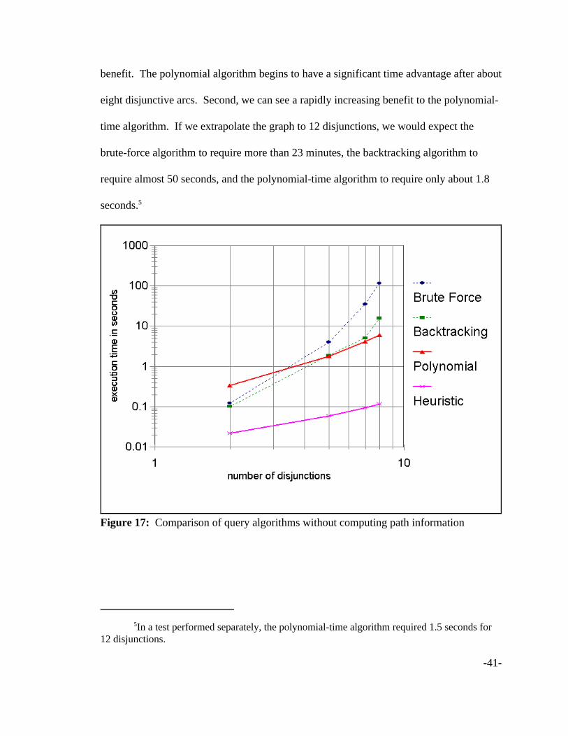
5In a test performed separately, the polynomial-time algorithm required 1.5 seconds for12 disjunctions.
-41-
Figure 17: Comparison of query algorithms without computing path information
benefit. The polynomial algorithm begins to have a significant time advantage after about
eight disjunctive arcs. Second, we can see a rapidly increasing benefit to the polynomial-
time algorithm. If we extrapolate the graph to 12 disjunctions, we would expect the
brute-force algorithm to require more than 23 minutes, the backtracking algorithm to
require almost 50 seconds, and the polynomial-time algorithm to require only about 1.8
seconds.5
-42-
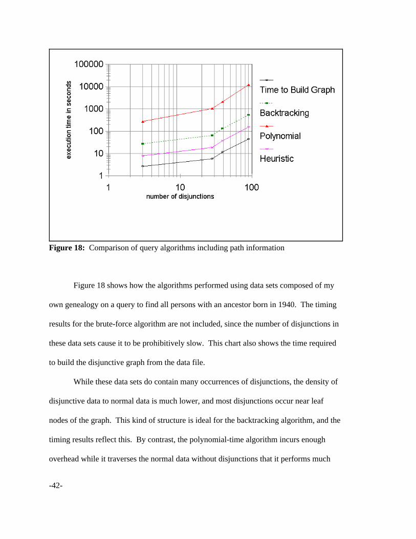
Figure 18: Comparison of query algorithms including path information
Figure 18 shows how the algorithms performed using data sets composed of my
own genealogy on a query to find all persons with an ancestor born in 1940. The timing
results for the brute-force algorithm are not included, since the number of disjunctions in
these data sets cause it to be prohibitively slow. This chart also shows the time required
to build the disjunctive graph from the data file.
While these data sets do contain many occurrences of disjunctions, the density of
disjunctive data to normal data is much lower, and most disjunctions occur near leaf
nodes of the graph. This kind of structure is ideal for the backtracking algorithm, and the
timing results reflect this. By contrast, the polynomial-time algorithm incurs enough
overhead while it traverses the normal data without disjunctions that it performs much
-43-
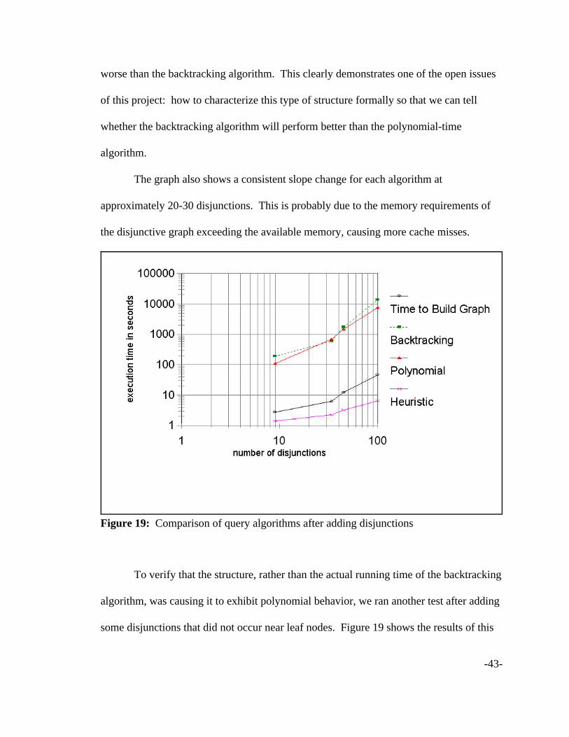
Figure 19: Comparison of query algorithms after adding disjunctions
worse than the backtracking algorithm. This clearly demonstrates one of the open issues
of this project: how to characterize this type of structure formally so that we can tell
whether the backtracking algorithm will perform better than the polynomial-time
algorithm.
The graph also shows a consistent slope change for each algorithm at
approximately 20-30 disjunctions. This is probably due to the memory requirements of
the disjunctive graph exceeding the available memory, causing more cache misses.
To verify that the structure, rather than the actual running time of the backtracking
algorithm, was causing it to exhibit polynomial behavior, we ran another test after adding
some disjunctions that did not occur near leaf nodes. Figure 19 shows the results of this
-44-
test, which confirm that the backtracking algorithm performs much worse with this type
of disjunction.
Both sets of results reflect the polynomial-time behavior of the new algorithm;
however, they also reflect a great deal of overhead for executing the algorithm on large
files with few disjunctions. In addition, this type of query that requires the algorithm to
trace through all the ancestors introduces more complexity. Since this query cannot be
done with a set of paths to enumerate every possible relationship between ancestors (i.e.
“Parent”, “Parent.Parent”, “Parent.Parent.Parent”, etc.), we used a query method where
we would first find the regular transitive closure of the node without path information,
thus finding all ancestors. We then run the algorithm again on the results to find all date
information for each ancestor. We effectively execute the algorithm twice.
To use the polynomial algorithm on typical large files in the range of several
megabytes or several gigabytes, we need to use more optimizations, both in building the
disjunctive graph and in querying it. Also, a more efficient method of finding a person’s
ancestors that doesn’t require us to execute the algorithm twice would greatly decrease
the running time required.
In addition, neither graph reflects the exponential time complexity of the
backtracking algorithm. Most of the disjunctions in the genealogy data we used occur
close to leaf nodes in the depth-first search, such as days or years of events; rather than
closer to the root node of the search. Since this behavior is highly dependent on the
structure of the data, we also tested the algorithms on randomly generated data. The
number of nodes in each graph varied from 5 to 18, and the number of edges was set to
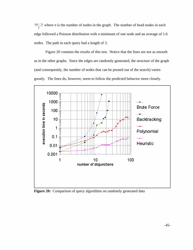
-45-
Figure 20: Comparison of query algorithms on randomly generated data
where n is the number of nodes in the graph. The number of head nodes in eachn n( )− 12
edge followed a Poisson distribution with a minimum of one node and an average of 1.6
nodes. The path in each query had a length of 3.
Figure 20 contains the results of this test. Notice that the lines are not as smooth
as in the other graphs. Since the edges are randomly generated, the structure of the graph
(and consequently, the number of nodes that can be pruned out of the search) varies
greatly. The lines do, however, seem to follow the predicted behavior more closely.

-46-
-47-
Chapter 6
Conclusions, Limitations, and Future Work
6.1 Summary
We have applied an algorithm to compute the transitive closure of a node in a
disjunctive graph to answer queries on disjunctive databases. We modified this algorithm
to keep track of path information. We have shown that under certain conditions, this
algorithm works correctly and can still run in polynomial time.
We have also established a model for representing disjunctive data in XML, and
we have built a prototype database to store and query this data. Empirical tests verify that
actual running times agree with theoretical predictions.
6.2 Limitations and Future Work
This project raises as many issues as it answers. While we have established a set
of conditions under which we can perform queries in polynomial time, many theoretical
questions still remain unanswered, including the following.
• When the graph is sparse enough, an algorithm such as the backtracking algorithm
does not require much time, even though worst-case analysis shows it to be slow.
Can we characterize the structure of a given disjunctive graph to show when an
exponential algorithm is still good enough, like in [ST01]?
• Can we represent more complicated structures, and can we apply the polynomial-
time algorithm to query them? These are two examples:

-48-
• Suppose that a we want to create a data table listing all of a user’s
ancestors that migrated from Illinois to Utah, and suppose that one
ancestor might have been born in Illinois before they left (in which case,
this ancestor should be included) or in Utah after they arrived (in which
case, the ancestor should not be included). This disjunction spans multiple
tables, so how might we represent this data, and would it satisfy the
conditions for the polynomial-time algorithm?
• Suppose that we need to add a disjunctive edge representing something
like (a OR b) Y ((c AND d) OR e), rather than (a OR b) Y (c OR d OR e),
as our current model of disjunctive edges allows. How would we
represent and query this sort of edge?
• Are there different ways we could represent the same disjunctive data? Could
some of these be more efficient than other ways, in terms of storage space, data
redundancy, and query complexity? Could we develop some kind of normal form
for disjunctive data, with these questions in mind?
• Is there a better way we can detect graphs with disjunctive edges that match at
more than one position in the path, and can we do it in polynomial time? Is there
a way we can still execute queries on these graphs in polynomial time?
Other questions dealing strictly with the extra logic involved with disjunctions in
the database include the following.

-49-
• How can we implement the different types of updates for incomplete data, such as
those described in [AG85] and [KW85]?
• How do we handle a query that contains variables, such as “find all records of
people with a father X, such that X was born in 1800 and the father of X was born
in 1770”?
• Can we do a pattern-matching search on the text in our disjunctive database, such
as SOUNDEX or regular expression? Is the complexity affected if all of the
nodes in a disjunction match the search pattern?
• Is there an efficient way to convert currently-existing data into disjunctive data? It
takes a lot of time to generate test data from an existing data file. While files that
contain “dirty” data exist, they depend mostly on natural language processing to
understand what the disjunctive values are, and it is difficult to specify a certain
pattern for converting then into <Disj> form. Automated data extraction
techniques would be very useful. Some problems to consider, including examples
of these problems actually found in the test data, are:
• How do we extract all possible values, if a given entry is invalid? e.g.
Date: 19 045 1779, which I took to mean “month 04 or month 05” but not
“month 45.”
• When do we factor in common substrings of a value? e.g. Date: 01
1734/35, which means “1734 or 1735,” so we have to factor in the “17” to
both the “34” and the “35.” We must also take care to distinguish this type
-50-
of entry from an entry like 01 1734/1735, where no factoring is necessary,
and like 01/02/1734, where no disjunction is even intended.
• What do we do if a very large range of values matches an entry? e.g. Date:
22 07 19??. It would be very inefficient to store each year from 1900-
1999 individually. Perhaps we could narrow the range through other clues
in the record (which is another question in itself), but if the range is still
too large, perhaps we should consider allowing statistical distributions as
values. How could we represent something like that?
• What if an entry is ambiguous? e.g. Date: 09/10 1652. Does the ‘/’
character indicate a disjunction, as in “month 09 or month 10”, or is it a
delimiter, as in “day 09 and month 10”? Also, does 11/13 11 1087 mean
“11 or 13”, or “between 11 and 13”?
• What if natural language processing is necessary? e.g. Date: ABT. 1490,
or Date: BEF. 1490. Should we be able to recognize all possible
abbreviations of “about,” “before,” “after,” “circa,” etc.? Related to this,
what if a disjunction is indicated by a note, e.g. Death Place: Provo, Utah.
Note: Could have also died at Pleasant Grove, Utah, or at Lindon, Utah.
A few questions related to the prototype implementation arise also, including the
following.
• Can we do any query optimization, making better use of indexes, or caching
results and partial results from the reachability matrix? If we know that there are

-51-
relatively few disjunctions in a data file, can we add a preprocessing step while
querying the data to take advantage of the data that doesn’t have disjunctions? If
the results are too big for main memory, how can we store partial results on disk?
Is query planning affected by the presence of disjunctive edges? For example, one
join order might involve an edge with a disjunctive tail, but a different join order
might not.
• Can we implement this with a more general query language, such as those
described in [XQUERY] or [DFFLS99]? If the query language allows
disjunctions within the query, could that affect the running time? There is
certainly more logic involved with disjunctions in the query. Normally, using
relational algebra notation, FA|B r = FA r c FB r, but with disjunctive data this
equality does not hold. For example, consider Figure 6, and consider the query
FDate.Day=“12” | Date.Day=“13” EventRec. The record shown in Figure 6 should be returned
in this query, since the day is either “12” or “13,” which in either case matches the
selection. If we separate the query and execute FDate.Day=“12” EventRec and
FDate.Day=“13” EventRec individually, however, nothing will be returned, since the
record does not satisfy either selection criteria alone.
• Can we make the prototype into a more general database that is not genealogy-
centered? What other applications are there for this work?

-52-
-53-
Bibliography
[AG85] S. Abiteboul and G. Grahne, “Update Semantics for IncompleteDatabases”, Proceedings of the 11th International Conference on VeryLarge Databases (VLDB), Aug. 21-23, 1985, Stockholm, Sweden, pp. 1-12.
[DFFLS99] A. Deutsch, M. Fernandez, D. Florescu, A. Levy, D. Suciu, “A QueryLanguage for XML,” Proceedings of the Eighth International World WideWeb Conference, May 11-14, 1999, Toronto, Canada.
[DOM] “Document Object Model (DOM)” The World Wide Web Consortium(W3C), http://www.w3c.org/DOM/.
[GED02] “GEDCOM XML Specification, Release 6.0, Beta Version,” Family andChurch History Department of The Church of Jesus Christ of Latter-DaySaints, http://www.familysearch.org/GEDCOM/GedXML60.pdf, Dec. 6,2002.
[IV89] T. Imielinski and K. Vadaparty, “Complexity of Query Processing inDatabases with OR-Objects,” Proceedings of the Eighth ACM Symposiumon Principles of Database Systems (PODS), Mar. 29-31, 1989,Philadelphia, Pennsylvania, pp. 51-65.
[KW85] A. M. Keller and M. W. Wilkins, “On the Use of an Extended RelationalModel to Handle Changing Incomplete Information”, IEEE Transactionson Software Engineering, Vol. 11, No. 7, Jul. 1985, pp. 620-633.
[LYY95] J. Lobo, Q. Yang, C. Yu, G. Wang, and T. Pham, “Dynamic Maintenanceof the Transitive Closure in Disjunctive Graphs,” Annals of Mathematicsand Artificial Intelligence, Vol. 14, 1995, pp. 151-176.
[NIAGARA] “Niagara Query Engine,” University of Wisconsin,http://www.cs.wisc.edu/niagara/.
[SHORE] “Shore Object Repository,” University of Wisconsin,http://www.cs.wisc.edu/shore/.
[ST01] D. A. Spielman and S. H. Teng, “Smoothed Analysis: Why The SimplexAlgorithm Usually Takes Polynomial Time,” Proceedings of the Thirty-Third Annual ACM Symposium on Theory of Computing, Jul. 6-8, 2001,Crete, Greece, pp. 296-305.
-54-
[TDCZ00] F. Tian, D. DeWitt, J. Chen, and C. Zhang, “The Design and PerformanceEvaluation of Alternative XML Storage Strategies”, ACM SIGMODRecord Special Issue on Data Management Issues in E-Commerce, Vol.31, No. 1, Mar. 2002, pp. 5-10.
[XERCES] “Xerces C++ Parser,” The Apache XML Project,http://xml.apache.org/xerces-c/index.html.
[XML] “Extensible Markup Language (XML)” The World Wide Web Consortium(W3C), http://www.w3c.org/XML/.
[XQUERY] “XQuery 1.0: An XML Query Language” The World Wide WebConsortium (W3C), http://www.w3c.org/TR/xquery/.