r 2017 - banco de la república (banco central de colombia) · predict average annual in ation were...

- Bogotá - Colombia - Bogotá - Colombia - Bogotá - Colombia - Bogotá - Colombia - Bogotá - Colombia - Bogotá - Colombia - Bogotá - Colombia - Bogotá - Colombia - B

cmunozsa

Texto escrito a máquina

Clustering and forecasting inflation expectations using the World Economic Survey: the case of the 2014 oil price shock on inflation targeting countries

cmunozsa


Por: Hector M. Zarate-Solano Daniel R. Zapata-Sanabria

cmunozsa


Núm. 993 2017

Clustering and forecasting inflation expectations using the World

Economic Survey: the case of the 2014 oil price shock on inflation

targeting countries ∗

Hector M. Zarate-Solano† Daniel R. Zapata-Sanabria‡

April 27, 2017

Abstract

This paper examines inflation expectations of the World Economic Survey for ten inflation

targeting countries. First, by a Self Organizing Maps methodology, we cluster the trajectory of

agents inflation expectations using the beginning of the oil price shock occurred in June of 2014 as

a benchmark in order to discriminate between those countries that anticipated the shock smoothly

and those with brisk changes in expectations. Then, the expectations are modeled by artificial

neural networks forecasting models. Second, for each country we investigate the information

content of the quantitative survey forecast by comparing it to the average annual inflation based

on national consumer price indices. The results indicate the presence of heterogeneity among

countries to anticipate inflation under the oil shock and, also different patterns of accuracy to

predict average annual inflation were found depending on the observed inflation trend.

Key Words: Inflation expectations, machine learning, self-organizing maps, nonlinear auto-

regressive neural network, expectation surveys

JEL Classification: C02, C222, C45, C63, E27

∗We would like to thank Johanna Garnitz at the IFO Institute for Economic Research for providing the data usedin this paper. The findings and suggestions expressed in this paper are those of the authors and do not necessarilyrepresent the view of the Banco de la Republica or its board of Directors†Senior Econometrician at Banco de la Republica Colombia (Central Bank of Colombia), email:

[email protected]‡Research Assistant at Banco de la Republica Colombia (Central Bank of Colombia), email:

[email protected] ff

1

mailto: [email protected]

mailto: [email protected]

1 Introduction

Subjective data from economic expectations surveys across countries has contributed recently on

studying crucial empirical macroeconomic issues focused on expectations formation and forecasting.

Expectations serves as guidance for real economic variables and policy decision makers and specifically,

inflation expectations are crucial for countries where targeting inflation were implemented as the

monetary policy rule. In general , their usefulness is considered on various kinds of tasks. For

instance, to test theories of inflation rigidities, to estimate key structural parameters, to test the

public understanding of the monetary policy. In addition, inflation expectations serve as a predictor

variable in both macroeconomic models and business cycles turning points forecasting models.

Expectation surveys have been applied to different agents, which include economic experts,

central bankers, financial agents, consumers, and firms. The implementation helps to provide a stock

of data that could be converted into an informational source about the effectiveness of the economic

policies and the economic agents level of institutional confidence. In the inflation expectations case,

surveys advise to the monetary policy makers about anchoring of inflation. One source to obtain

those expectations is through the World Economic Survey (WES), which is conducted among more

than 1000 economic experts in approximately 120 countries. The respondents evaluate the present

economic situation and the outlook of their own country given special attention to price trends

answering qualitative and quantitative questions.

In this sense, we pay particular attention to analyze a sample of inflation targeting countries and

take into account the oil price shock of 2014 on their inflation expectations and other macroeconomic

indicators due to their oil dependency as exporters or importers. With this aim, the forecast

evaluation takes place after the oil’s shock period from the 2014.QIII to 2016.QII. Also, for a better

understanding of agents’ expectations behavior and to obtain optimal forecasts, the combination

between clustering and forecasting analysis can be used synergistically. Thus, data visualization

techniques are useful to discover relevant characteristics and to perform clustering of agents’

expectations. Furthermore, machine learning methodologies could be employed to forecast inflation

expectations based on qualitative questions of WES surveys.

The objective of this article is twofold: firstly, we rely on Claveria et al. (2016) (1) , and

make use of the Self-organizing maps, SOM, as a clustering technique on the agent’s expectations

for some targeting countries to discriminate them after the oil’s shock of 2014 between soft or brisk

behaviors. Then, we predict the inflation expectations evaluating, at different horizons, the forecasts

from different models specifications of the Non-linear Autoregressive Neural network (NAR-NN).

Secondly, we examine the informational content of the quantitative prediction of the average annual

inflation on the WES in order to obtain further reliable inflation forecasts.

2

This paper contains five sections apart from this introduction. In the second section, the

methodologies of the models for clustering and forecasting are presented, emphasizing in the neural

network techniques. Section 3 described the expert economic survey data and how the qualitative

expectations indicators were aggregated. In section 4, we presented the main results, including

the clustering analysis and forecasting accuracy. Next in section 5, the statistical evaluation

of the quantitative inflation question is assessed. Finally, conclusions and future extensions are

proposed.

2 Methodology

This section describes the clustering and forecasting methodologies from the point of view of machine

learning methodologies from which artificial neural networks models have been widely used due

to their abilities to fulfill these tasks. The most frequent model in clustering is the Kohoens

Self-organizing maps, SOM, and to forecasting the multilayer perceptron from which the Non-linear

autoregressive neuronal network, NAR-NN, is a subclass.

2.1 Artificial neural networks

In order to explain the ANNs framework, we start looking at the key points of the simple neural

network model that are the base of the SOM and NAR-NN models.

ANNs are a kind of parallel computing systems consisting of a number of simple interconnected

processors called neurons or nodes, which through a learning process adjust their parameters to

approximate non-linear functions between a set of inputs (variables) and the output (results), see

Jain et al. (1996) (2). Thus there is not required assumptions about the generating process data

which allowed them to be a more flexible model.

Following Hagan et al. (2016) (3), the simplest neuron model is composed by a scalar input p,

called a single variable, which is multiplied by a scalars weight w. Then, wp plus the bias b form the

called net input n, which is send to the activation function f, to produce the scalar neuron output

a. However, ANN’s architecture may be more complex, they can have multiple inputs, layers and

neurons as show the figure 1.

3

Figure 1: A three layer neural network. Based on Hagan et al (2014)

The parameters, weights and biases, are adjusted with some learning rule (eg. kohonen’s

learning rule), and the activation function is chosen according the task wanted to solve. For example,

in the case of the SOM, were used the Competitive function. This networks are feed forward, which

means that there no loops between outputs and inputs 1. To see more details about ANNs see

Hagan et al. (2016) (3).

2.2 Self-organizing maps

In this paper, the Self-organized Maps, proposed by Kohonen 1982, are used to cluster the economic

agents’ expectations before the oil’s shock and mapping those expectations after the shock in the

resulting cluster map. SOMs are competitive feed-forward networks based on unsupervised training

with the property of topology preservation, which means that nearby input patterns should be

represented on the map by nearby output units, see Kohonen (2001) (4).

The SOM architecture consists of a two layer network: in the first layer the inputs are

multiplied with weights, that were initialized as small numbers. Then the results are evaluated by a

competitive function that produce a wining neuron (Best Matching unit). The weights are updated

according a learning rule, equation (1), and the neuron’s neighborhood are updated too. See the

figure (2) below.

wi(q) = (1− α)wi(q − 1) + α(p(q)) (1)

The training stage for each iteration consists in adjusting the weighs of the winning neuron

and its neighbors by using the learning rule. This process guarantees similarity between the inputs

1In the NAR-NN Model to perform multi-steps forecasts the network is transformed into a recurrent network aftertheir parameters were trained as a feed forward network.

4

Figure 2: A Self-Organizing Map of 5x5 dimension. Based on Hagan et al (2014)

and the neurons that are represented on the feature map (the second layer of the map). At the end

of the process the resulting learned weights capture the data characteristics on the feature map that

have two dimensions (3).

Kohonen suggested to use rectangular and hexagonal neighborhoods. Furthermore, with the

aim of improving the SOM’s performance, we considered to gradually decrease the neighbor size

during the training progresses, until it only includes the winning neuron. Also, to take into account

the trade-off between fast learning and stability, the learning rate can be also decreased in this

phase. This is given by the fact that a high learning rate at the beginning of the training phase

allows a quick but unstable learning. On the other side, with a small rate, the learning becomes

slow but more stable.

2.3 Nonlinear auto-regressive neural network

In this subsection we describe the main issues of the NAR-NN methodology which includes the

training algorithm selected. The model assumes that the current observation could be explained by

the compromise of two components: the signal and the noise. The first is an unknown function that

is approximated by the neural network to the inflation expectation time series with an autoregressive

structure. The second component is the noise, which is assumed to be independent with zero mean.

The model equation is stated below:

Yt = g(Yt−1 + Yt−2 + . . .+ Yt−p) + et (2)

In order to obtain the best approximation for g , the neural network architecture should

meet the following three conditions: it has to avoid overfitting 2, the predicted error should be

2 Overfitting is a characteristic that should be avoided and occurs when the neural network fit the data closely in

5

uncorrelated through time, and the cross-correlation function between the predicted errors and the

observed time series should be close to zero. In this paper we rely on the Bayesian regularization

framework to approximate g in a parsimonious way.

The objective function for the Bayesian regularization setup is given by:

F (x) = βT∑t=1

(Yt − Yt)T (Yt − Yt) + αn∑

i=1

x2i (3)

Which is the weighted combination between the model fit and the smoothness. The parameter

α penalizes the model complexity and β reflect the goodness of fit. The term x2i is the sum squared

of the parameters values of the network, weights and biases.

Using the Bayesian theorem sequentially, the joint posterior distribution of the parameters α

and β given the data D and the neural network model chosen M , is computed by multiplying the

likelihood times the joint a-priori distribution of α and β divided by the evidence:

P (α, β|D,M) =P (D|α, β,M)P (α,B|M)

P (D|M)(4)

The a priori joint density for α and β is assumed to come from the uniform distribution.

Consequently, the posterior could be obtained by computing the following probabilities:

P (D|α, β,M) =P (D|X,β,M)P (X|α,M)

P (X|D,α, β,M)(5)

P (X|D,α, β,M) =P (D|X,β,M)P (X|α,M)

P (D|α, β,M)(6)

to see the technical details and the full training algorithm see Hagan et al (2016) (3)

The adaptation of the algorithm requires to set the neural network architecture, M , which

means we have to pick the number of neurons in the input layer, the number of hidden layers, the

number of neurons per hidden layer and the number of neurons in the output layer, to more details

see Zhang et al (1998) (5).

Bayesian regularization guarantee that the parameters sum is optimal for the given data. In

order to optimize the regularization parameters the objective function F (x) should be minimized

following the Levenberg-Marquardt Back propagation algorithm.

Given the Bayesian regularization results there is flexibility to model the architecture of the

the training set, but in the testing set and out of sample, the fitting is poor.

6

network. For the hidden layer, we set a fix number of nodes, where their parameters, weights and

biases, always will sum a small amount. We used just one hidden layer due to the length of the

series. We observed that an extra layer did not change significantly the results. With respect to the

output layer, one node is used because the forecast is one-step-ahead. The selection of the adequate

number of input nodes or lags will be explained in the NAR-NN results section. In order to improve

the generalization of the network, the methodology usually requires to divide the data into three

sets: the training, validation and testing. However, the Bayesian regularization avoid the validation

stage because the solution is based on the optimization of the equation (3).

We employed the hyperbolic Tangent Sigmoid as activation function for the nodes in the

hidden layer as is showed below, which is frequently used in forecasting.

a =en − e−n

en + e−n(7)

a = n (8)

To the output layer the linear function is used. Notice that before training the network, data

normalization, which transform the data in the interval between [-1, 1], is required to faster the

training algorithm.

pn =2(p− pmin)

(pmax − pmin)− 1 (9)

3 World economic survey data

The data source of our empirical analysis came from the World economic Survey (WES) applied by

the IFO Institute for Economic Research.

The surveys contain qualitative and quantitative questions related to diagnostics and expec-

tations covering different macroeconomic topics: economic growth, interest rates, consumption,

capital, exchange rates and inflation, among others 3. These opinion surveys are responded quarterly

by economic experts mostly from public and private sector and academy. The subjective response

could be classified as positive, neutral or negative. These opinions are analyzed by assigning values

to the responses in the following way: where the response is considered positive a numerical value

of 9 is coded. A value of 5 represent a neutral choice and a value of 1 express the negative response.

Next, the average rating is calculated by country for each question. Traditionally the analysts divide

by the following rule: a positive zone is related to an average greater than 5, and the negative is

3 An example of the World economic survey WES questionnaire was include in the appendix A, see figure 12

7

below to 5. Nevertheless, the neutral zone depends on the subjectivity of the analyst. One of results

of this paper is to establish the limits of the three zones by letting the data speaks for itself.

The WES survey also introduce a quantitative questions about the future inflation. This

question is also evaluated through the forecasting error decomposition in the section 6. To see more

about WES see Stangl (2007) (6, chap. 5), and Stangl(2007) (7).

For SOM and NAR-NN models we rely on the qualitative WES questions. Thus, we select

expectations of the next six months for 16 inflation targeting countries around the world that ranges

from 1991.QIII to 2016.QII. The sample of countries analyzed were Brazil, Canada, Switzerland,

Chile, Colombia, Czech Republic, United Kingdom, Hungary, Korea Republic, Mexico, Norway,

Philippines, Poland, Sweden, Thailand, South Africa. In figure 5 the inflation expectations indicator

and the actual annual inflation are plotted for some countries of the sample 4 5. In addition we

include a summarize of or data, their histograms, and their correlation, relevant to the SOM analysis

6. Furthermore, we applied traditional unit root tests to study the properties of the inflation

expectations time series, see the results on table A.7 in appendix A.

Overall economy Capital expenditures Private consumption Inflation rate

Min 1 1 1 1

1stQ 4.8 4.7 4.57 4

Median 5.8 5.7 5.5 5.5

Mean 5.79 5.59 5.44 5.32

3rdQ 6.8 6.6 6.5 6.8

Max 9 9 9 9

Table 1: Data Summary of WES expectations

4We did not include all the inflation targeting countries in our study because the survey for them stared at thedifferent dates

5Figure 11 in Appendix A contains the full time series length6Figure 3 shows that our variables have variation, figure 4 shows the correlation between them. Because we are

interested in inflation expectation and the other variables do not show a linear correlation with it, we keep them toour analysis.

8

Figure 3: Histograms of Agents’ expectations of economic situation for next 6 months in macroeco-nomic variables

Figure 4: Scatter plot of of Agents’ expectations of economic situation for next 6 months

9

(a) Brazil (b) Canada

(c) Chile (d) Colombia

10

(e) Czech Republic (f) Korea

(g) Mexico (h) Norway

11

(i) Switzerland (j) United Kingdom

Figure 5: Countries Inflation Expectations and Annual inflation. Source WES survey and OECD statistics12

4 Results

In this section we present the main results of the different methodologies related to clustering and

forecasting the inflation’s expectation. First, we present the SOM analysis, which include sequential

steps: the map topology choice based on data, the SOM neural network training and validation and

finally the clustering map of agents expectations. These three steps are explained in detail in the

appendix B. Then we overlap agents’ inflation expectations on the resulting SOM map. By last, the

NAR-NN results are developed.

4.1 Self-organizing maps of agents’ expectations

Based on the SOM analysis we set a 10X10 hexagonal map with a learning rate varying from 0.05

to 0.0001 and we used 1000 iterations. The computation was realized using the kohonen package

in R developed by Wehrens et al. (2007) (8). The training step used observations before the oil

shock identified on 2014.QII, which cover a sample of 84 observations per country for the expected

situation by the end of the next 6 months of the overall economy, capital expenditures, private

consumption and inflation.

A key tool in this analysis is the feature map or heat map that is the representation of a single

variable across the map (Figure 6). In this application, the colors identify the level of the indicator.

For example: the blue color is associated with low expectations and the red with high expectations.

Clustering can be performed by using hierarchical clustering on the weight learned vectors of the

variable. This procedure requires to set the number of clusters. Thus, given the nature of the

expectations we used 3 clusters that represents the low, neutral and high expectations.

(a) Overall economy (b) Capital expenditures

13

(c) Private consumption (d) Inflation rate

Figure 6: SOMs of countries economy situation expectations for the next 6 months (1991.QIII to2014.QIV )

4.2 Overlapping agents’ inflation expectations by country

In order to discriminate the agents’ inflation expectation patterns after the oil price shock that

took place on June of 2014, we overlap those expectation from the third quarter of 2014 to the

second quarter of 2016 on the heatmap resulting from the SOM analysis. As a consequence, we

classified the expectations patterns by country into two categories: smooth and brisk expectations

trajectories. For smooth transitions we expected to found a path that moves through a single cluster.

Otherwise, we identify a brisk trajectory by observing a changing path among several clusters. In

The figure 7(a), the black arrow represent the trajectory of the inflation expectation with an initial

node marked with a black start symbol.

For example, in the case of Colombia, figure 7(d), the observed inflation expectations on July

of 2014 are located in the higher expectation cluster, then moves through the Heatmap ending in

the lower expectation cluster. We classified this pattern as having brisk expectations behavior. On

the other hand, the Korea Republic Inflation expectations (f) remains in the same neutral cluster.

Therefore it is classified with a smooth expectation path. Finally, the summary of the classification

results for the sample of countries expectations is shown in table 2.

14



(e) Czech Republic (f) Korea Republic

15



Figure 7: Countries Inflation rate next 6 months (III.2014 to II.2016) on the Expected Inflationrate SOM Map

16

Country Inflation expectation Lag selected

Brazil Brisk 1

Canada Brisk 8

Chile Smooth 4

Colombia Brisk 5

Czech R. Smooth 6

Korea R. Smooth 2

Mexico Smooth 6

Norway Smooth 1

Switzerland Brisk 8

United K. Smooth 6

Table 2: Classification of inflation expectations and lag selected in the NAR-NN model

4.3 Non linear autoregressive neural network results

From the Bayesian regulation framework applied to the NAR-NN methodology, we have to select a

model M . For each country, the sum of parameters is conditional on the complexity of its data.

In this context we chose a flexible network where regularization guarantee the minimum sum of

parameters. Thus, we set an architecture with one hidden layer of 10 neurons. Moreover, at the

input layer we have to specify the number of neurons, that corresponds to the lag order used to

forecast one step ahead. We used the Neural Network Toolbox provided by Matlab (9) .

The lag order selection were based on different criterion’s: The mean squared error resulting

from the testing data, the error auto-correlation function, and the cross-correlation between the

errors and the observed data. In this way, from lags 1 to 10 we generated 30 neural networks per lag

and obtain the MSE for the training, testing, and the complete sample. Then, we select the lag that

reports the smallest median from the testing data sample taking into account the auto-correlations

diagnostics 7. The lag chosen for each country is presented in table 2 and the overall results from

lags 1 to 10 are shown in table 3 8. A similar procedure was developed by Ruiz et al. (2016)

(10).

Figure 8 displays the observed data (Black line), the fit in the training set (Blue line), the

forecasts in horizons 1 and 2 (green and orange lines respectively), and the out of sample forecasts 8

steps ahead (yellow line). Also, the figure 9 is divided into three blocks. The left corresponds to

7In most of the cases mean and median, of the lag chosen, are both the smallest. However, in Colombian, CzechR., and Switzerland is not the case, even though the lag’s mean is closes to the smallest mean.

8These results for all data set, training set and testing set are presented in tables C.8, C.9, and C,10 respectivelyin appendix C.

17

the training set (from 1991.QIII to 2014.QII), the center to the testing set, which is the after oil

shock period (from 2014.QIII to 2016.QII), and the right block is the forecasted period. The table 4

contains the mean squared error at different time horizons for the selected countries 9 10.

Countries Lags 1 2 3 4 5 6 7 8 9 10

Brazil mean 1.70 2.08 1.85 1.93 1.83 1.85 1.83 1.90 1.92 2.04

median 1.69 2.07 1.85 1.86 1.83 1.85 1.83 1.84 1.92 2.04

Canada mean 2.02 1.74 1.59 1.63 1.62 1.54 1.56 1.52 1.75 1.73

median 2.03 1.74 1.59 1.63 1.62 1.54 1.56 1.52 1.75 1.73

Switzerland mean 1.32 1.22 1.04 1.04 1.02 0.98 1.06 0.78 0.93 0.77

median 1.31 1.22 1.04 1.04 1.02 0.98 1.06 0.78 0.94 0.83

Chile mean 4.36 2.76 2.75 2.69 2.73 2.82 2.90 3.18 3.13 2.92

median 4.38 2.76 2.79 2.68 2.76 2.81 2.88 3.28 3.08 2.91

Colombia mean 4.94 2.88 2.91 2.95 2.89 2.88 2.96 3.26 3.20 3.30

median 4.97 2.88 2.92 2.88 2.78 2.83 2.81 3.23 3.15 3.20

Czech R. mean 0.73 0.74 0.73 0.70 0.93 0.72 1.20 1.24 2.21 1.61

median 0.74 0.74 0.73 0.70 0.93 0.67 1.20 1.24 2.10 1.16

United K. mean 0.86 0.87 0.95 0.95 0.88 0.82 0.84 1.21 0.87 0.85

median 0.87 0.86 0.95 0.95 0.88 0.82 0.83 0.84 0.87 0.83

Korea R. mean 2.21 1.86 1.99 2.02 2.03 2.21 2.40 2.06 2.06 2.05

median 2.22 1.86 1.99 2.02 2.03 2.21 2.40 2.06 2.06 2.05

Mexico mean 0.38 0.43 0.52 0.49 0.48 0.34 0.48 0.35 0.52 1.09

median 0.38 0.42 0.52 0.49 0.48 0.30 0.57 0.37 0.31 0.53

Norway mean 1.41 1.44 1.61 1.67 1.59 2.01 2.04 2.10 1.88 1.80

median 1.41 1.44 1.61 1.67 1.59 2.01 2.04 2.10 1.88 1.80

Table 3: Lag statistics test data - forecast one-step ahead. sample = 30

9A summary results of the neural networks parameters are presented in table C.11, appendix C10A simulation of 1000 networks was performed to ensure that the MSE presented belongs to the average neural

network find after specifying the model previous described. See table C.12, appendix C

18



19



20


Figure 8: Countries forecasted Inflation rate next 6 months by NAR-NN

Figure 9: Data block division ant out of sample sets

21

All data Training set Testing set Testing setone steap-ahead one-step ahead one-step ahead two-step ahead

Brazil 1,993 2,039 1,470 2,616Canada 1,320 1,301 1,519 1,834Chile 2,226 2,185 2,680 2,429Colombia 1,573 1,462 2,776 2,648Czech R 0,887 0,908 0,665 1,464Korea 1,474 1,440 1,857 3,028Mexico 0,896 0,951 0,299 0,341Norway 1,846 1,884 1,419 1,221Switzerland 0,313 0,268 0,781 1,414United K. 1,215 1,252 0,820 1,465

Table 4: MSE by period and time horizon

5 Quantitative forecasting inflation expectations

This section look at the comparison between annual average inflation based on the CPI and the

correspondent quantitative WES inflation assessment which is obtained from the survey question

“the rate of inflation on average this year will be: % p.a.”. In this section we follow previous works

by Fildes and Stekler (2002) (11) and Hammella and Haupt (2007) (6, chap. 9) in order to quantify

and examine the accuracy of the WES forecasts at different horizons. It is worth to notice that the

expert’s information increase from quarter to quarter as data inflation is released.

5.1 Statistical analysis of the forecasting error

The forecast error is calculated in the following way:

e(L,Q(h), t) = p(L, t)− q(L,Q(h), t) (10)

Where L = countries, h = I,II,III,IV, and t = 1991,. . . , 2016 First, we compute different error

statistics for each quarter that include the RMSFE (root mean squared forecast error), MAE (mean

absolute error), and Theil U-statistic, See Hammella and Haupt 2007 11.

Second, the error decomposition, based on the mean squared error and proposed by Theil

in 1966 (12), is constructed . This illustrated how the error changes conditional on the different

forecasting horizons and is divided into three factors: the bias share Vh, the spread share Sh, and

11The the respective statistics equations are presented in appendix D.1, also MAE and U-statistic results are intables D.13 and D.14 respectively, see appendix

22

the covariance share Kh. The Vh bias component refers to the systematic distortions of the forecast,

where bias should decrease through forecast horizons only if the expectations are anchored. The

Sh measures the dispersion between the observed inflation and the WES forecast . Finally, Kh

assess the linear association between the average inflation and the WES forecast, if the correlation

is perfect then K = 0. Notice that The three components should add 1.

5.2 Quantitative inflation expectations results

The tables 5 and 6 summarize the RMSFE and its decomposition for the countries selected in

previous sections at the different time horizons. According with the results the RMSFE decrease

through the year for countries such as Switzerland, Colombia, Korea, and Norway. Nevertheless,

there are some countries which shows another pattern where the last forecast is more uncertain such

as Brazil, Canada, Chile, Czech Republic, and United Kingdom. These features remain observing

the MAE and U-statistics. Figure 10 compare the respective observed annual inflation (bar line)

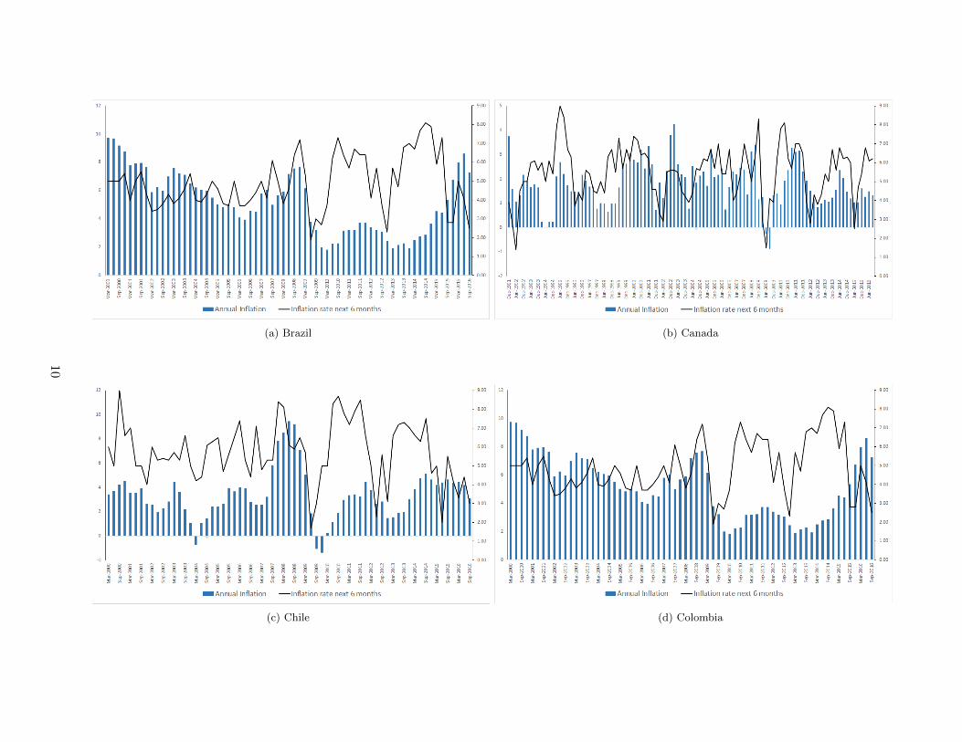
and the WES expectation for each quarter by countries 12 13.

In Colombia we observed that the actual annual inflation was overestimated during the

period 2000 to 2003, then until 2007 the expectations were close to the observed inflation. The

2008 financial crises caused that expectations suffers a short period of underestimation and over

estimation till 2014. Finally, the 2014 oil shock induce an underestimated inflation period. There

are different patterns across the countries such as Mexico, where the expectations were close to the

actual inflation until the oil shock, after the inflation was overestimate.

Countries 4-step forecast (QI) 3-step forecast (QII) 2-step forecast (QIII) 1-step forecast (QIV)

Brazil 182.71 321.48 354.44 431.01

Canada 0.70 0.57 0.42 0.58

Switzerland 0.75 0.50 0.41 0.38

Chile 1.23 1.46 1.36 1.66

Colombia 1.80 1.67 1.43 1.00

Czech R. 2.29 1.16 1.32 2.02

United K. 0.89 0.88 0.90 0.99

Korea 1.61 1.41 1.16 1.09

Mexico 3.37 2.03 4.48 3.62

Norway 0.78 0.65 0.52 0.39

Table 5: Root mean squared forecast errors of WES survey quantitative inflation question

12 Due to there are some countries with different monetary policies regimens the starting year of the series whereadjusted for the scale

13The quarter-specific forecasting error by country is plotted in Figure 17, appendix D

23

Countries Error descomposition 4-step forecast (QI) 3-step forecast (QII) 2-step forecast (QIII) 1-step forecast (QIV)

Brazil

V 0.13 0.06 0.07 0.01

S 0.84 0.81 0.53 0.10

K 0.06 0.14 0.45 0.92

Canada

V 0.16 0.20 0.31 0.16

S 0.05 0.14 0.26 0.26

K 0.83 0.70 0.46 0.61

Switzerland

V 0.22 0.32 0.30 0.19

S 0.22 0.28 0.37 0.54

K 0.60 0.55 0.35 0.31

Chile

V 0.003 0.02 0.05 0.02

S 0.02 0.20 0.74 0.75

K 1.02 0.84 0.25 0.27

Colombia

V 0.003 0.06 0.04 0.01

S 0.08 0.02 0.05 0.33

K 0.96 0.99 0.95 0.71

Czech R.

V 0.10 0.17 0.05 0.0001

S 0.05 0.38 0.35 0.36

K 0.88 0.60 0.64 0.68

United K.

V 0.23 0.26 0.18 0.14

S 0.16 0.28 0.43 0.30

K 0.64 0.56 0.43 0.60

Korea

V 0.37 0.44 0.52 0.39

S 0.03 0.002 0.0003 0.02

K 0.62 0.45 0.50 0.62

Mexico

V 0.03 0.13 0.01 0.01

S 0.43 0.002 0.11 0.03

K 0.57 1.04 0.92 1.01

Norway

V 0.06 0.02 0.08 0.02

S 0.19 0.14 0.13 0.18

K 0.79 0.79 0.83 0.84

Table 6: Theil error decomposition of the WES forecast errors 1991.I to 2016.II

24



25



26


Figure 10: Countries Inflation Expectations and Annual inflation. Source WES survey and OECD statistics27

6 Conclusions

Predicting inflation expectations from international survey data applied to economics agents is a

valuable goal in some empirical topics of monetary macroeconomics. The quarterly questions about

the evolution of prices in these surveys consider both qualitative and quantitative answers. In this

research, we started with analyzing the informational content of the subjective question by finding

different patterns of expectations among countries and forecasting it. Secondly, we evaluate the

suitability of the quantitative WES inflation forecasts by accomplishing a statistical decomposition

of the forecasting errors.

Thus, we first rely on explorative techniques situated inside the machine learning methods

to cluster and predict inflation’s expectations in a sample of countries that have implemented the

inflation targeting scheme as their monetary policy. Therefore, by using a clustering technique

known as Self-Organizing Maps and a predictive model based on artificial neuronal networks, we

visualize and predict different patterns of inflation expectations according to their perceptions before

the imminent coming oil shock that took place in the middle of 2014.

We cluster 16 countries according to the evolution of their inflation expectations during the

transition period to the recent minimum oil price mark. Then we generate forecasts of survey

expectations by the NAR-NN model for selected countries. Regarding to the SOM analysis, we

find that some countries exhibited a brisk behavior that is associated with signs that inflation

expectations were deanchoring. On the other side, there were countries with a soft evolution of

inflation expectations.

Concerning to the statistical evaluation of the quantitative inflation expectation, we detected

that the uncertainty of the predictions of the average annual inflation across countries could be

classified into two groups of countries with different patterns through the year. The first group is

characterized by the fact that the closer the economic agent is to the end of the year the smaller the

prediction bias is. It includes Colombia and Switzerland among others. The other group of countries

which attract attention by displaying an increasing bias in the last quarter of the prediction are

Brazil, Canada and Chile. However, we have to notice that overestimation of inflation is observed

for some countries in periods when inflation is going down.

28

7 Bibliography

[1] O. Claveria, E. Monte, S. Torra, A self-organizing map analysis of survey-based agents ex-

pectations before impending shocks for model selection: The case of the 2008 financial crisis,

International Economics 146 (2016) 40–58. doi:10.1016/j.inteco.2015.11.003.

[2] A. Jain, J. Mao, K. Mohiuddin, Artificial neural networks: a tutorial, Computer 29 (3) (1996)

31–44. doi:10.1109/2.485891.

[3] M. T. Hagan, H. B. Demuth, M. H. Beale, J. O. De, Neural network design, s. n., 2016.

[4] T. Kohonen, Self-organizing maps, Springer, 2001.

[5] G. Zhang, B. E. Patuwo, M. Y. Hu, Forecasting with artificial neural networks:: The state of

the art, International Journal of Forecasting 14 (1) (1998) 35 – 62. doi:http://doi.org/10.

1016/S0169-2070(97)00044-7.

URL http://www.sciencedirect.com/science/article/pii/S0169207097000447

[6] G. Goldrian, Handbook of Survey-Based Business Cycle Analysis, Edward Elgar, 2007.

[7] A. Stangl, European data watch: Ifo world economic survey micro data, Schmollers Jahrbuch :

Journal of Applied Social Science Studies / Zeitschrift fur Wirtschafts- und Sozialwissenschaften

127 (3) (2007) 487–496.

URL http://EconPapers.repec.org/RePEc:aeq:aeqsjb:v127_y2007_i3_q3_p487-496

[8] R. Wehrens, L. Buydens, Self- and super-organising maps in r: the kohonen package, J. Stat.

Softw. 21 (5).

URL http://www.jstatsoft.org/v21/i05

[9] M. T. Hagan, H. B. Demuth, M. H. Beale, Neural Network Toolbox User’s Guide.

[10] L. Ruiz, M. Cuellar, M. Calvo-Flores, M. Jimenez, An application of non-linear autoregressive

neural networks to predict energy consumption in public buildings, Energies 9 (9) (2016) 684.

doi:10.3390/en9090684.

[11] R. Fildes, H. Stekler, The state of macroeconomic forecasting, Journal of Macroeconomics

24 (4) (2002) 435–468. doi:10.1016/s0164-0704(02)00055-1.

[12] H. Theil, G. A. C. Beerens, C. G. d. Leeuw, C. B. Tilanus, Applied economic forecasting,

North-Holland, 1975.

[13] Self-organising maps for customer segmentation using r (Feb 2014).

URL https://www.r-bloggers.com/self-organising-maps-for-customer-segmentation-using-r

29

http://dx.doi.org/10.1016/j.inteco.2015.11.003

http://dx.doi.org/10.1109/2.485891

http://www.sciencedirect.com/science/article/pii/S0169207097000447


http://dx.doi.org/http://doi.org/10.1016/S0169-2070(97)00044-7

http://dx.doi.org/http://doi.org/10.1016/S0169-2070(97)00044-7


http://EconPapers.repec.org/RePEc:aeq:aeqsjb:v127_y2007_i3_q3_p487-496

http://EconPapers.repec.org/RePEc:aeq:aeqsjb:v127_y2007_i3_q3_p487-496

http://www.jstatsoft.org/v21/i05

http://www.jstatsoft.org/v21/i05

http://dx.doi.org/10.3390/en9090684

http://dx.doi.org/10.1016/s0164-0704(02)00055-1

https://www.r-bloggers.com/self-organising-maps-for-customer-segmentation-using-r

https://www.r-bloggers.com/self-organising-maps-for-customer-segmentation-using-r

Appendix A Data

A.1 Qualitative series

Brazil

From 1991−07−01 to 2016−04−01

Infla

tion

rate

nex

t 6 m

onth

s

1995 2000 2005 2010 2015

24

68

Canada

From 1991−07−01 to 2016−04−01

Infla

tion

rate

nex

t 6 m

onth

s

1995 2000 2005 2010 2015

24

68

Swirtzeland

From 1991−07−01 to 2016−04−01

Infla

tion

rate

nex

t 6 m

onth

s

1995 2000 2005 2010 2015

24

68

Chile

From 1991−07−01 to 2016−04−01

Infla

tion

rate

nex

t 6 m

onth

s

1995 2000 2005 2010 2015

24

68

Colombia

From 1991−07−01 to 2016−04−01

Infla

tion

rate

nex

t 6 m

onth

s

1995 2000 2005 2010 2015

24

68

Czech republic

From 1991−07−01 to 2016−04−01

Infla

tion

rate

nex

t 6 m

onth

s

1995 2000 2005 2010 2015

24

68

United Kingdom

From 1991−07−01 to 2016−04−01

Infla

tion

rate

nex

t 6 m

onth

s

1995 2000 2005 2010 2015

24

68

Korea

From 1991−07−01 to 2016−04−01

Infla

tion

rate

nex

t 6 m

onth

s

1995 2000 2005 2010 2015

24

68

Mexico

From 1991−07−01 to 2016−04−01

Infla

tion

rate

nex

t 6 m

onth

s

1995 2000 2005 2010 2015

24

68

Norway

From 1991−07−01 to 2016−04−01

Infla

tion

rate

nex

t 6 m

onth

s

1995 2000 2005 2010 2015

24

68

Figure 11: Expected Inflation Rate for the next 6 months

30

A.2 WES Survey questionnaire

Figure 12: Example of the World economic survey WES questionnaire

31

A.3 Unit root tests

ADF Phillips-Perron

t-Stat Prob. t-Stat Prob.

Brazil -5.32 0.0001 -5.25 0.0002

Canada -5.37 0.0001 -5.40 0.0001

Switzerland -4.49 0.0026 -4.09 0.009

Chile -4.97 0.0005 -4.97 0.0005

Colombia -6.15 0.0000 -6.14 0

Czech Republic -4.62 0.0017 -4.73 0.0012

United Kingdom -4.89 0.0007 -4.63 0.0016

Korea -5.62 0.0000 -5.55 0.0001

Mexico -5.06 0.0004 -4.89 0.0007

Norway -5.21 0.0002 -5.03 0.0004

Test critical values: 1% level -4.04 -4.053392

5% level -3.45 -3.455842

10% level -3.15 -3.15371

Table 7: Unit root test

Appendix B Self- organizing map validation

B.1 Choice of Topology

In this section we set the for the best topology according with the available data. It includes finding

the dimensions of the map and the form of the neighbourhood. In order to have more neighbors

around the winning neuron, we choose the hexagonal topology that allocate six neurons around .

for the dimensions we found several empirical rules. The first rule is to have the number of neurons

increase as the square root y of the number of data points. This give us a map of 40 neurons. The

second rule said to have 10 samples per neuron, that give of 192 neurons around.

Trying to get enough granularity on the map with also a small topographic error, we tried

different architectures. Unfortunately, there is not a firm criterion for the best performance in SOM

networks. Due the goal of finding the agent’s clusters before the oil’s shock price, we divide our data

into two sets, before and after the shock. Thus, the training data will be from the third quarter of

1991 to the second quarter of 2014.

While The first rule suggest a map of 16x12, by the square rule suggested to have a map with

32

38 neurons around. Using the R software, we analyzed various architectures: from 3x10 to 18x10,

from which their topographic errors where stored, and taking into account the granularity and their

errors 14.Figure 3(a) bring us to choose hexagonal topology of 10x10.

(a) Best Matching unit error, error node distance, quantization error and sample per neuron vs

map width node size

(b)

Figure 13

14The quantization error is not comparable between maps because is susceptible to map size. To see more abouttopographic error see Post-training analysisi section

33

B.2 Post-training analysis

Following Wehrens (2007) (8) and Lynn (2014) (13) we analysis the results from the trained map

to validated the previous results. The training progress shows the mean distance between neuron’s

weights to the samples represented through each iteration. When the training progress reach a

minimum, no more iterations are required, see figure 3(b).

(a) (b)

Figure 14

In figure 4(a) the node or quality distance map is shown. This map displays an approximation

of the distance per node to the sample that their are representing. The smallest the distance,a

better map is found. This error is called the quantization error. When it is large, there are some

inputs vectors that are not adequately represented on the map. However it is susceptible to the

map sizes: if the map is too large, it could be near to zero. This would represent overfitting because

the number of neurons on the map should be significantly smaller that the sample size. the mean

quantization error found is 0.5888693.

In the figure 4(b) can analyse how many samples are mapped to each node on the map. Ideally

we want that the sample distributions be relatively uniform. Our map is relatively uniform, and it

is mapping between 10 to 15 samples per neuron. Also, there are non empty neurons.

34

(a) (b)

Figure 15

The figure 5(b) map is also named the U-matrix, and shows the distance between each neuron

and its immediate neighbours. Because we choose a hexagonal neighbour, each neuron have six

neurons on their neighbourhood. This maps also assists to identify similar neurons. Before analyse

our Neighbourhood distance, it is helpful the figure 5(a) that shows neighbourhood distance per

neuron on the total map, in this case the neuron number 45.

Figure 16: Weight vectors

35

The weight vectors plot, figure 6, shows the weights associated to each neuron. Each weight

vector is similar to the variable that is representing due to the kohonen’s learning rule. Looking the

weights distribution on the map, green for economy over all, yellow for Capital expenditures, orange

for private consumption, and white for inflation expectations, we can distinguish patterns of the

variables. In our map we can see how the inflation expectations is dissimilar to the other Agent’s

expectations, and the latter how they are similar to each others.

Finally we present three measures of topographic errors. We already saw the first one,the

quantization error, that is average distance between each variable and the closest neuron , again

our quantization error is 0.5888693. The Best-matching error is the average distance between the

best matching unit and the following, which is 1.568656, this is in terms of coordinates in the map.

Similarly, the node distant error is the average distance between all pairs of most similar codebook

vectors., which is 1.387984.

Appendix C Non Linear Autorregresive neural networks valida-

tion

C.1 Lag selection

36

Countries Lags 1 2 3 4 5 6 7 8 9 10

Brazil mean 2.02 1.99 1.88 1.94 1.90 1.86 1.87 1.92 1.89 1.88median 2.01 1.99 1.88 1.90 1.90 1.86 1.87 1.88 1.89 1.88

Canada mean 1.17 1.38 1.31 1.29 1.33 1.30 1.31 1.32 1.29 1.32median 1.15 1.38 1.31 1.29 1.30 1.30 1.31 1.32 1.29 1.30

Switzerland mean 1.03 1.09 1.04 1.04 1.03 1.03 0.76 0.31 0.50 0.63median 1.03 1.09 1.04 1.04 1.03 1.03 0.87 0.31 0.50 0.83

Chile mean 2.22 2.09 2.10 2.22 2.09 1.97 2.08 2.05 2.05 2.10median 2.22 2.09 2.05 2.23 2.17 1.95 1.93 1.97 2.11 2.10

Colombia mean 1.56 1.58 1.58 1.62 1.62 1.60 1.61 1.60 1.57 1.62median 1.56 1.58 1.58 1.59 1.57 1.59 1.55 1.58 1.54 1.57

Czech Republic mean 1.85 2.05 1.99 1.94 1.85 0.93 1.73 1.78 0.36 0.26median 1.87 2.06 1.99 1.94 1.85 0.89 1.73 1.78 0.32 0.25

United Kingdom mean 1.27 1.40 1.39 1.38 1.26 1.21 1.10 0.96 1.15 0.96median 1.27 1.41 1.39 1.38 1.26 1.21 1.10 1.00 1.16 0.92

Korea mean 1.36 1.47 1.45 1.46 1.45 1.35 1.36 1.30 1.29 1.31median 1.36 1.47 1.45 1.46 1.45 1.35 1.36 1.30 1.29 1.31

Mexico mean 1.26 1.36 1.33 1.14 1.12 0.99 1.21 1.26 0.95 0.27median 1.25 1.37 1.32 1.14 1.12 0.90 1.44 1.35 1.21 0.25

Norway mean 1.87 2.08 1.97 1.98 1.92 1.91 1.83 1.81 1.76 1.75median 1.86 2.08 1.97 1.98 1.92 1.91 1.83 1.81 1.76 1.75

Table 8: Lag statistics all data - forecast one step ahead- sample = 30

37

Countries Lags 1 2 3 4 5 6 7 8 9 10






Czech Republic mean 1.95 2.17 2.11 2.05 1.94 0.95 1.78 1.83 0.18 0.13median 1.96 2.17 2.10 2.05 1.94 0.91 1.78 1.83 0.15 0.16

United Kingdom mean 1.31 1.45 1.43 1.42 1.29 1.25 1.13 0.93 1.18 0.97median 1.31 1.46 1.43 1.42 1.29 1.25 1.13 1.01 1.18 0.92

Korea mean 1.29 1.44 1.40 1.41 1.39 1.27 1.26 1.23 1.22 1.23median 1.28 1.44 1.40 1.41 1.39 1.27 1.26 1.23 1.22 1.23



Table 9: Lag statistics train data - forecast one step ahead- sample = 30

38

Countries Lags 1 2 3 4 5 6 7 8 9 10






Czech R. mean 0.73 0.74 0.73 0.70 0.93 0.72 1.20 1.24 2.21 1.61median 0.74 0.74 0.73 0.70 0.93 0.67 1.20 1.24 2.10 1.16

United K. mean 0.86 0.87 0.95 0.95 0.88 0.82 0.84 1.21 0.87 0.85median 0.87 0.86 0.95 0.95 0.88 0.82 0.83 0.84 0.87 0.83

Korea R. mean 2.21 1.86 1.99 2.02 2.03 2.21 2.40 2.06 2.06 2.05median 2.22 1.86 1.99 2.02 2.03 2.21 2.40 2.06 2.06 2.05



Table 10: Lag statistics test data - forecast one step ahead- sample = 30

39

C.2 Post training analysis

Countries Total number Effective number maximum sum Sum squared Totalof parameters of parameters squared of parameters of parameters epoch

Brazil 31 2.88 2760 1.74 355Canada 101 7.66 53 1.01 622Chile 61 4.68 91.3 1.11 228Colombia 71 5.02 72 0.72 1000Czech Republic 81 31.17 61.6 20.96 314Korea 41 2.99 280 1.10 1000Mexico 81 20.71 61.7 9.91 114Norway 31 2.96 2760 1.49 70Switzerland 101 38.81 53.4 22.16 330United Kingdom 81 10.20 64.7 3.39 245

Countries Best Error Input-error Correlation coefficientepoch autocorrelation correlation Trainig R Testing R All R

Brazil 2 1 0 0.605 0.877 0.632Canada 99 1 0 0.570 0.334 0.551Chile 56 1 0 0.702 -0.049 0.678Colombia 429 1 0 0.445 0.560 0.463Czech Republic 253 1 0 0.885 0.607 0.884Korea 1000 1 0 0.523 -0.464 0.554Mexico 64 1 0 0.875 0.474 0.879Norway 4 1 0 0.641 -0.041 0.640Switzerland 240 1 0 0.935 0.759 0.921United Kingdom 77 1 0 0.740 0.473 0.743

Table 11: Neural networks resume results of training phase

C.3 MSE evaluation

Brazil Korea

All data Training set Testing set All data Training set Testing set

mean 2.01 2.05 1.65 1.47 1.44 1.86

median 2.00 2.04 1.61 1.47 1.44 1.86

std 0.04 0.03 0.18 0.01 0.01 0.03

maximum 2.09 2.09 2.11 1.52 1.44 2.51

minimum 1.92 1.97 1.24 1.36 1.34 1.62

40

Canada Mexico


mean 1.33 1.31 1.52 0.97 1.03 0.34

median 1.32 1.30 1.52 0.90 0.95 0.30

std 0.06 0.06 0.01 0.24 0.24 0.17

maximum 2.09 2.09 2.11 3.91 4.00 2.94

minimum 1.92 1.97 1.24 0.90 0.95 0.30

Chile Norway


mean 2.21 2.17 2.69 1.87 1.91 1.41

median 2.23 2.18 2.68 1.86 1.90 1.42

std 0.06 0.07 0.03 0.04 0.04 0.03

maximum 1.33 1.36 1.01 2.06 2.12 1.51

minimum 0.55 0.54 0.67 1.82 1.86 1.25

Colombia Switzerland


mean 1.59 1.48 2.83 0.31 0.27 0.78

median 1.57 1.46 2.78 0.31 0.27 0.78

std 0.08 0.07 0.21 0.00 0.00 0.00

maximum 1.93 1.76 3.69 0.31 0.27 0.78

minimum 1.57 1.46 2.77 0.31 0.27 0.78

Czech Republic United Kigdom


mean 0.90 0.92 0.69 1.21 1.25 0.82

median 0.89 0.91 0.67 1.21 1.25 0.82

std 0.08 0.08 0.08 0.00 0.00 0.00

maximun 1.21 1.25 0.82 1.21 1.25 0.82

minimum 1.21 1.25 0.82 1.21 1.25 0.82

Table 12: Neural network simulations statistics by data sets, sample = 1000

41

Appendix D Quantitative forecasting inflation expectations

D.1 Equations of the statistical analysis forecasting error

Root mean squared forecast error (RMSFE):√√√√ 1

26

2016∑1991

e(L,Q(h), t)2 (11)

Mean absolute error (MAE):

1

26

2016∑1991

| e(L,Q(h), t) (12)

Theil U.statistic: √126

∑20161991 e(L,Q(h), t)2√

126

∑20161991 q(L,Q(h), t)2

√126

∑20161991 p(L, t)

2(13)

Bias share:

V (h) =

[126

∑20161991 q(L,Q(h), t)2 − 1

26

∑20161991 p(L, t)

]2

126

∑20161991 e(L,Q(h), t)2

(14)

The spread share:

S(h) =[Sq(h)− Sp(h)]2

126

∑20161991 e(L,Q(h), t)2

(15)

where Sq(h) and Sp(h) are the standard deviations of the respective quarter.

The covariance share:

K(h) =2(1− rq,p(h))Sq(h)− S(h)

126

∑20161991 e(L,Q(h), t)2

(16)

where rq,p(h) is the correlation coefficient between q and p. Thus V (h) + S(h) +K(h) = 1

42

4-step forecast (QI) 3-step forecast (QII) 2-step forecast (QIII) 1-step forecast (QIV)

Brazil 67.52 99.05 94.00 122.19

Canada 0.51 0.43 0.34 0.41

Switzerland 0.59 0.41 0.32 0.30

Chile 0.97 1.04 0.89 0.93

Colombia 1.33 1.14 0.92 0.65

Czech R. 1.43 0.78 0.82 0.95

United K. 0.76 0.72 0.68 0.77

Korea 1.26 1.11 0.91 0.78

Mexico 1.63 1.22 2.14 1.79

Norway 0.61 0.51 0.43 0.31

Table 13: MAE of WES survey quantitative inflation question

4-step forecast (QI) 3-step forecast (QII) 2-step forecast (QIII) 1-step forecast (QIV)

Brazil 0.001 0.001 0.001 0.001

Canada 0.138 0.113 0.083 0.115

Switzerland 0.237 0.162 0.126 0.120

Chile 0.022 0.028 0.027 0.033

Colombia 0.010 0.009 0.007 0.005

Czech R. 0.049 0.026 0.029 0.048

United K. 0.110 0.111 0.112 0.122

Korea 0.075 0.067 0.055 0.054

Mexico 0.022 0.011 0.022 0.019

Norway 0.143 0.118 0.101 0.079

Table 14: U-statistic of WES survey quantitative inflation question

43

(a)

(b)

44

(c)

(d)

45

(e)

(f)

46

(g)

(h)

47

(i)

(j)

Figure 17: Quarter-specific forecasting error by country

48

ogotá -

r 2017 - banco de la república (banco central de colombia) · predict average annual in ation were...

Documents