r. kraus, e. cliﬀ, c. woolsey, and j. luby · 2009-06-02 · r. kraus, e. cliff, c. woolsey, and...

OPTIMAL CONTROL OF AN UNDERSEA GLIDER IN ASYMMETRIC PULL-UP

R. Kraus, E. Cliff, C. Woolsey, and J. Luby

aCASVirginia Center for Autonomous Systems

Virginia Polytechnic Institute & State UniversityBlacksburg, VA 24060www.unmanned.vt.edu

October 24, 2008

Technical Report No. VaCAS-2008-03Copyright c© 2008

The views expressed in this article are those of the author and do notreflect the official policy or position of the United States Air Force, De-partment of Defense, or the U.S. Government.

Summary

An undersea glider is a winged autonomous undersea vehicle which modulates its buoyancyto rise or sink and moves its center of mass to control pitch and roll attitude. By properlyphasing buoyancy and pitch control, an undersea glider rectifies the vertical motion causedby changes in buoyancy into forward motion caused by the lift force on the fixed wing. Thecharacteristic “porpoising” motion is useful in oceanographic surveys and the propulsionmethod is extremely efficient – undersea gliders routinely operate for months without humanintervention. Glider efficiency could be improved even further by addressing the phenomenonof “stall” (loss of lift) when a glider transitions from downward to upward flight. Becausethe stall phenomenon occurs asymmetrically over the vehicle’s wing, it can cause directionalerrors which must be corrected at a corresponding energetic cost. This paper describes theformulation of a point mass model and its dynamic equations of motion. An optimal controlformulation was designed using angle of attack and buoyancy as controls to investigate controlscheduling methods for avoiding stall in a symmetric pull-up. The calculations were repeatedusing three different numerical solution techniques for comparison of the methodologies andresults. The model was updated to include longitudinal rigid body dynamics and changedthe control to the rate of change of the longitudinal center of gravity location. This modelallowed for the inclusion of added mass effects due to fluid displacement.

i

Contents

1 Introduction 1

2 Vehicle Dynamic Model 2

2.1 Equations of Motion . . . . . . . . . . . . . . . . . . . . . . . . . . . . . . . 2

2.2 Wings Level Gliding Flight . . . . . . . . . . . . . . . . . . . . . . . . . . . . 4

3 Longitudinal Dynamics: Point Mass Model 5

4 Optimal Control Problem 6

4.1 Necessary Conditions . . . . . . . . . . . . . . . . . . . . . . . . . . . . . . . 7

4.2 Two-Point Boundary Value Problem . . . . . . . . . . . . . . . . . . . . . . 7

4.3 Numerical Results . . . . . . . . . . . . . . . . . . . . . . . . . . . . . . . . . 7

4.4 Alternative Solution Methods . . . . . . . . . . . . . . . . . . . . . . . . . . 11

5 Longitudinal Dynamics: Rigid Body Model 12

6 Conclusions 15

ii

List of Figures

1 Reference frames. . . . . . . . . . . . . . . . . . . . . . . . . . . . . . . . . . 2

2 Equilibrium glide characteristics for the Slocum model in [1]. . . . . . . . . . 5

3 Control histories for four values of tf (RU = Rα = 100). . . . . . . . . . . . . 8

4 State histories for four values of tf (RU = Rα = 100). . . . . . . . . . . . . . 9

5 Control histories with tf = 30 seconds for three choices of RU/Rα. . . . . . . 9

6 State histories with tf = 30 seconds for three choices of RU/Rα. . . . . . . . 10

7 Three-state solution method comparison. . . . . . . . . . . . . . . . . . . . . 12

8 Fixed rate model comparison with optimized models. . . . . . . . . . . . . . 14

9 Trajectory Comparisons. . . . . . . . . . . . . . . . . . . . . . . . . . . . . . 14

10 Solution including added mass effects. . . . . . . . . . . . . . . . . . . . . . . 15

iii

List of Tables

1 Initial and final equilibrium states. . . . . . . . . . . . . . . . . . . . . . . . 13

iv


1 Introduction

Buoyancy-driven undersea gliders are highly efficient winged underwater vehicles which lo-comote by modifying their internal shape. In the typical actuation scheme, a servo-actuatorshifts the center of mass relative to the center of buoyancy and a buoyancy bladder modulatesthe glider’s net weight (weight minus buoyancy). By appropriately cycling these actuators,the vehicle can control its directional motion and propel itself with great efficiency. Examplesof undersea gliders include Slocum [13], Seaglider [3], and Spray [12].

Undersea gliders locomote by repeatedly descending and ascending in a sawtooth pattern.The locomotive efficiency owes to the fact that these vehicles spend much of their time insteady, gliding flight. Little control effort is required except at transition points, where theglider switches from downward to upward flight or vice versa. Early efforts to design flightcontrol systems for undersea gliders focused, appropriately, on designing efficient steadymotions and controlling the vehicles about these nominal motions [4]. More recent studies[6] have re-examined undersea glider design and control with a view toward even greaterefficiency in nominal flight.

The transition from descent to ascent is a minor portion of an undersea glider’s flight profileand has received little attention in flight control design. In this maneuver, the vehicletransitions from a stable, steady descending motion to a stable, steady ascending motionwhile maintaining forward flight. The locomotive force (i.e., the net weight) changes sign andthe vehicle rotates by moving its center of mass. Graver [5] proposed a nine-state switchedlinear state feedback controller to negotiate the transition and illustrated the results in asimulation of Slocum. As Graver pointed out, however, existing undersea glider controlsystems are not so sophisticated. Typically, the net weight and center of mass are servo-controlled to pre-set positions that correspond to desired steady motions. “Flight control”consists of outer loop corrections to attain the desired pitch and heading angles [5]. Whilethis approach works well for a vehicle in steady motion, operators have observed problemswith stall when vehicles transition from descent to ascent. When this happens, the vehiclecan lose directional stability, a situation which must be corrected with additional controleffort when the vehicle finally approaches the desired steady, ascending flight condition [3].

This report uses an optimal control formulation to investigate control scheduling for anundersea glider in a symmetric pull-up. The motivation is to generate and characterizefeasible state/control histories which involve a transition from steady, descending flight tosteady, ascending flight. A primary objective is to prevent stall during this maneuver.The results may suggest a more informed open-loop control scheduling strategy for existingundersea glider flight control systems.

The initial findings in this report were presented at the 18th International Symposium onMathematical Theory of Networks & Systems [7].

Section 2 develops the general dynamic model for an undersea glider and reviews the con-ditions for steady, wings level flight. Section 3 describes a simplified longitudinal dynamicmodel that is amenable to numerical optimization. Section 4 describes the optimal controlformulation and presents the results of our numerical investigation. Conclusions and a brief

Page 1

Virginia Center for Autonomous Systems Report No. 2008-03


discussion of related, ongoing research efforts are provided in Section 6.

2 Vehicle Dynamic Model

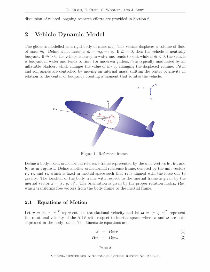
The glider is modelled as a rigid body of mass mrb. The vehicle displaces a volume of fluidof mass mf . Define a net mass as m = mrb − mf . If m = 0, then the vehicle is neutrallybuoyant. If m > 0, the vehicle is heavy in water and tends to sink while if m < 0, the vehicleis buoyant in water and tends to rise. For undersea gliders, m is typically modulated by aninflatable bladder, which changes the value of mf by changing the displaced volume. Pitchand roll angles are controlled by moving an internal mass, shifting the center of gravity inrelation to the center of buoyancy creating a moment that rotates the vehicle.

rcm

v

!

i 1

i2

i3

b1b

2

b3

Figure 1: Reference frames.

Define a body-fixed, orthonormal reference frame represented by the unit vectors b1, b2, andb3, as in Figure 1. Define another orthonormal reference frame, denoted by the unit vectorsi1, i2, and i3, which is fixed in inertial space such that i3 is aligned with the force due togravity. The location of the body frame with respect to the inertial frame is given by theinertial vector x = [x, y, z]T . The orientation is given by the proper rotation matrix RIB,which transforms free vectors from the body frame to the inertial frame.

2.1 Equations of Motion

Let v = [u, v, w]T represent the translational velocity and let ω = [p, q, r]T representthe rotational velocity of the AUV with respect to inertial space, where v and ω are bothexpressed in the body frame. The kinematic equations are

x = RIBv (1)

RIB = RIBω (2)

Page 2



where the character · denotes the 3 × 3 skew-symmetric matrix satisfying ab = a × b forvectors a and b.

The rotation matrix RIB is typically parameterized using Euler angles. For aircraft andunderwater vehicles, the most common choice of Euler angles are the roll angle φ, the pitchangle θ, and the yaw angle ψ. Let e1, e2, and e3 represent the standard orthonormal basisfor R

3. In terms of conventional Euler angles, the rotation matrix is

RIB(φ, θ, ψ) = ee3ψee2θee1φ.

Another reference frame which is commonly used in ocean vehicle dynamics is the “currentframe,” known as the “wind frame” in aircraft dynamics (c1,c2, c3) . This frame is relatedto the body frame through the components of the body translational velocity vector. Definethe two hydrodynamic angles

α = arctan(wu

)and β = arcsin

( vV

), (3)

where V = ‖v‖. To transform a vector from the current frame to the body frame, one appliesthe proper rotation

RBC(α, β) = e−e2αee3β.

For example, one may transform the velocity vector from the current frame to the bodyframe as follows:

v = RBC(α, β)(V c1) =

V cosα cos βV sin β

V sinα cosβ

. (4)

The linear momentum of the body/fluid system, expressed in the body frame, is denotedp. The angular momentum is denoted h. The vectors p and h are the conjugate momentacorresponding to v and ω, respectively. Thus,

(p

h

)=

(M CT

C I

)(v

ω

)(5)

where the 3×3 sub-matrices M , C, and I define the 6×6 generalized inertia matrix, whichincludes both the rigid body inertia and the added inertia due to the fluid. The dynamicequations are

p = p × ω + mg(RT

IBi3

)+ f v(v,ω) (6)

h = h × ω + p × v +mrbgrcm ×(RT

IBi3

)+ mv(v,ω) (7)

where fv and mv represent the force and moment due to viscous flow effects and rcm isthe location of the vehicle center of mass. Typically, one writes f v in terms of its threecomponents in the current frame: drag force D, side force S, and lift force L. The viscousmoment is expressed in terms of its three components in the body frame: roll moment L,pitch moment M , and yaw moment N . Thus, we have

f v(v,ω) = −RBC(α, β)

D(v,ω)S(v,ω)L(v,ω)

and mv(v,ω) =

L(v,ω)M(v,ω)N(v,ω)

.

Page 3



Equations (1),(2), (6), and (7) describe the motion of a rigid undersea glider in inertial space.Given that our immediate aim is simply to characterize steady, wings level gliding motions,we have omitted the dynamics of the moving mass actuator from this model. In fact, inSection 3, we specialize further to a point mass model of the undersea glider, a standardpractice in flight trajectory optimization. For a higher-dimensional vehicle model, whichincludes the internal actuator dynamics, see [1] or [5].

In studying steady motions, we typically ignore the translational kinematics (1). Moreover,the structure of the dynamic equations (6) and (7) is such that only the “tilt vector”

ζ = RTIB

i3

is required to express the dynamics, allowing us to replace the matrix equation (2) for therotational kinematics with the equation for ζ. We therefore consider the following, reducedset of equations:

ζ = ζ × ω (8)

p = p × ω + mgζ + fv. (9)

h = h × ω + p × v +mrbgrcm × ζ + mv (10)

2.2 Wings Level Gliding Flight

The conditions for wings level, gliding flight are that ω = 0, v · e2 = 0, and ζ · e2 = 0. Thesecond condition implies that v = 0 and therefore that β = 0. The third condition impliesthat φ = 0. Assume a nominal velocity v0 = [u0, 0, w0]

T or, equivalently, nominal valuesof speed V0 and angle of attack α0. Substituting all of these conditions into equations (8)through (10), one obtains a corresponding center of mass location rcm, flight path angleγ0 = θ0 − α0, and net weight m0g; see [8] and references therein.

The equilibrium values of rcm, γ0, and m0 depend on the system parameters and on thelift and drag model as well as the speed and angle of attack. Let q(V ) denote the dynamicpressure:

q(V ) =1

2ρV 2

where ρ is the fluid density, which is assumed to remain constant. Let S represent a referencearea such as the wing planform area. Dimensional analysis shows that, in steady, symmetricflight, the drag and lift force may be written in terms of dimensionless coefficients as follows:

D(V, α) = CD(α)q(V )S and L(V, α) = CL(α)q(V )S

whereCD(α) = CD0

+K (CL(α))2 and CL(α) = CLαα.

Figure 2 shows the wings level equilibrium glide characteristics for the dynamic model givenin [1] for the Slocum electric glider with the wing surface area as the reference area: S =0.1327 m2. The lift and drag parameters are:

CLα= 2.04 rad−1, CD0

= 0.03, and K = 0.16.

Page 4



−30 −20 −10 0 10 20 30−80

−60

−40

−20

0

20

40

60

80

α ( o )

γ (

o ),θ

( o )

γθ

(a) θ(α) and γ(α).

−80 −70 −60 −50 −40 −30 −20 −10 0−80

−70

−60

−50

−40

−30

−20

−10

0

10

20

γ ( o )

θ (

o )

(b) θ versus γ.

Figure 2: Equilibrium glide characteristics for the Slocum model in [1].

Figure 2(a) illustrates a fundamental obstacle in transitioning an undersea glider from de-scending to ascending flight at constant speed: the equilibrium manifold is discontinuouswhen α is zero. There can be no “quasi-steady” transition from downward to upward flightat constant speed.

3 Longitudinal Dynamics: Point Mass Model

In this note, we consider only symmetric motions, i.e., motions confined to the vehicle’s planeof symmetry. Recalling that β ≡ 0 for longitudinally symmetric motions, we have from (4)

(VV α

)=

(cosα sinα− sinα cosα

)(uw

). (11)

Ignoring inviscid hydrodynamic coupling between pitch and heave motions, we find from thefirst and third components of equation (9) that

(muumww

)=

(−mwwqmuuq

)+ W

(− sin θcos θ

)−

(cosα − sinαsinα cosα

)(DL

)(12)

where W = mg.

At this point, we make a key assumption to simplify the optimal control problem developed inSection 4. We assume that mu = mw and, for notational simplicity, we define m = mu = mw.

While added mass is not generally the same in surge and heave for an undersea vehicle,the assumption considerably simplifies the optimal control problem formulation. Our aim isan improved understanding of control scheduling for an undersea glider in a pull-up and weexpect analysis results for this simplified model to provide valuable insight. Substituting (12)into (11), with mu = mw = m, the translational dynamic equations simplify to

(VV α

)=

(0V q

)+

1

mW

(− sin γcos γ

)−

1

m

(D(V, α)L(V, α)

)

Page 5



where γ = θ − α. For notational simplicity, we normalize the three forces by mass:

W =1

mW, D(V, α) =

1

mD(V, α), and L(V, α) =

1

mL(V, α).

Taking α and U = dWdt

as inputs, we have the following two-input dynamic model:

Vγ˙W

=

−W sin γ − D(V, α)1

V

(−W cos γ + L(V, α)

)

U

. (13)

4 Optimal Control Problem

We consider the model (13) of vertical plane motions for an undersea glider and study thecontrol of transition from dive to climb. It has been observed that such transitions canexhibit large angle of attack (AoA) values resulting in degraded heading stability [3]. It isof interest to find transition strategies that limit these AoA excursions.

In practice, the inputs (α and U) are subject to upper and lower bounds. In lieu of boundson the control, our cost functional will employ the usual quadratic integral (control effort)as follows:

J =1

2

∫ tf

0

(Rα

(α(t)

αref

)2

+RU

(U(t)

Uref

)2)

dt (14)

where Rα and RU are control penalty weights and αref and Uref are reference values. We takeαref = 1 radian and Uref = 1 (m/s2)/s. Initial conditions at time t0 = 0 and final conditionsat a specified final time t = tf are given for all three states:

V (t0) = V0, γ(t0) = γ0, W (t0) = W0 (15)

V (tf ) = Vf , γ(tf ) = γf , W (tf ) = Wf (16)

Our (open-loop) optimal control problem is to determine control histories α(·), U(·) totransfer the dynamic model (13) from initial conditions (15) to end conditions (16) whileminimizing the cost functional (14).

To study this problem we used Pontryagin’s Minimum Principle [9] to derive a two-pointboundary value problem (TPBVP) that characterizes extremal state/control trajectories.Numerical solutions of the TPBVP are candidates for optimality; they satisfy necessaryconditions for optimality. Our motivation here is to produce feasible state/control pathsthat meet the end conditions.

Page 6



4.1 Necessary Conditions

We begin with the usual variational Hamiltonian

H(λV , λγ, λW , V, γ, W , α, U)△= −λV

[D(V, α) + W sin γ

]+λγV

[L(V, α) − W cos γ

]

+λW U +λ0

2

(Rα

(α(t)

αref

)2

+RU

(U(t)

Uref

)2)

The adjoint vector (λV , λγ, λW ) must satisfy the differential equations:

λV = λV∂D

∂V−λγV

∂L

∂V+λγV 2

[L(V, α) − W cos γ

](17)

λγ = λV W cos γ −λγVW sin γ (18)

˙λW = λV sin γ +λγV

cos γ , (19)

whereas the Hmin optimality condition requires:

0 = −λV∂D

∂α+λγV

∂L

∂α+ λ0

Rα

α2

ref

α (20)

0 = λW + λ0

RU

U2

ref

U . (21)

As noted above, the drag coefficient is quadratic in α, so these equations are linear in the

controls. For a minimizer we must have λ0Rα

α2

ref

−2KC2

L α

mq(V (t))λV (t) ≥ 0. We assume

the problem is normal so that λ0 > 0 and test this minimality condition along candidateextremals.

4.2 Two-Point Boundary Value Problem

Using extremal controls from (20, 21) we have a system of six differential equations (13and 17-19) and six boundary conditions (15 and 16). We formulate a Newton problemwith the initial values of the adjoints as (three) unknowns and the end-conditions (16) tobe satisfied. This problem was solved numerically using the fsolve procedure in Matlab

(version R2007b). The underlying initial-value problem for the state/adjoint ODE systemwas solved using ode45.

4.3 Numerical Results

The problem of Section 4.2 was solved for a range of control weight ratios and final times.The lift and drag parameters, corresponding to the values used in [1] for the Slocum vehicle,are given near the end of Section 2.2. Other relevant parameters are:

m = 50 kg, S = 0.1327 m2, and ρ = 1027 kg/m3.

Page 7



The six boundary conditions (15 and 16) were the same for each case:

V0 = 0.77 m/s, γ0 = −12.7◦, W0 = 0.124 m/s2

Vf = V0, γf = −γ0, Wf = −W0

0 10 20 30 40 50 60−100

−80

−60

−40

−20

0

20

40

Time, t [s]

Buo

yanc

y P

ump

Rat

e [c

c/s]

tf = 30s

= 40s = 50s = 60s

(a) Pump rate history: U(t).

0 10 20 30 40 50 60−0.2

0

0.2

0.4

0.6

0.8

1

1.2

Time, t [s]

Com

man

ded

Ang

le o

f Atta

ck, α

[deg

])

tf = 30s

= 40s = 50s = 60s

(b) AoA history: α(t).

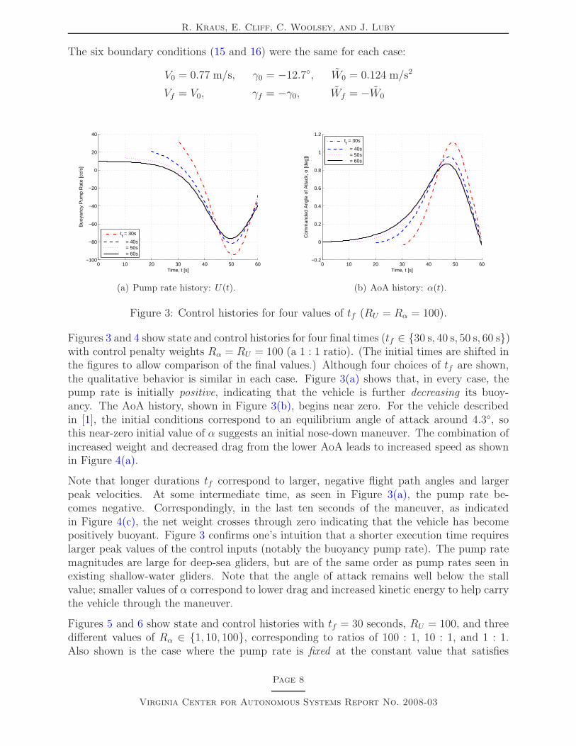
Figure 3: Control histories for four values of tf (RU = Rα = 100).

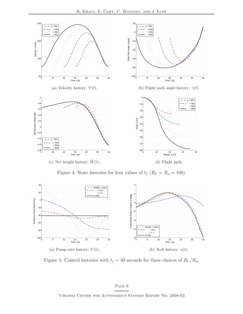
Figures 3 and 4 show state and control histories for four final times (tf ∈ {30 s, 40 s, 50 s, 60 s})with control penalty weights Rα = RU = 100 (a 1 : 1 ratio). (The initial times are shifted inthe figures to allow comparison of the final values.) Although four choices of tf are shown,the qualitative behavior is similar in each case. Figure 3(a) shows that, in every case, thepump rate is initially positive, indicating that the vehicle is further decreasing its buoy-ancy. The AoA history, shown in Figure 3(b), begins near zero. For the vehicle describedin [1], the initial conditions correspond to an equilibrium angle of attack around 4.3◦, sothis near-zero initial value of α suggests an initial nose-down maneuver. The combination ofincreased weight and decreased drag from the lower AoA leads to increased speed as shownin Figure 4(a).

Note that longer durations tf correspond to larger, negative flight path angles and largerpeak velocities. At some intermediate time, as seen in Figure 3(a), the pump rate be-comes negative. Correspondingly, in the last ten seconds of the maneuver, as indicatedin Figure 4(c), the net weight crosses through zero indicating that the vehicle has becomepositively buoyant. Figure 3 confirms one’s intuition that a shorter execution time requireslarger peak values of the control inputs (notably the buoyancy pump rate). The pump ratemagnitudes are large for deep-sea gliders, but are of the same order as pump rates seen inexisting shallow-water gliders. Note that the angle of attack remains well below the stallvalue; smaller values of α correspond to lower drag and increased kinetic energy to help carrythe vehicle through the maneuver.

Figures 5 and 6 show state and control histories with tf = 30 seconds, RU = 100, and threedifferent values of Rα ∈ {1, 10, 100}, corresponding to ratios of 100 : 1, 10 : 1, and 1 : 1.Also shown is the case where the pump rate is fixed at the constant value that satisfies

Page 8



0 10 20 30 40 50 6050

100

150

200

Time, t [s]

Vel

ocity

, V [m

/s]

tf = 30s

= 40s = 50s = 60s

(a) Velocity history: V (t).

0 10 20 30 40 50 60−100

−80

−60

−40

−20

0

20

Time, t [s])

Glid

e P

ath

Ang

le, γ

[deg

]

tf = 30s

= 40s = 50s = 60s

(b) Flight path angle history: γ(t).

0 10 20 30 40 50 60−0.8

−0.6

−0.4

−0.2

0

0.2

0.4

0.6

0.8

1

Time, t [s]

Net

Buo

yanc

y M

ass

[kg]

tf = 30s

= 40s = 50s = 60s

(c) Net weight history: W (t).

0 10 20 30 40−80

−70

−60

−50

−40

−30

−20

−10

0

Range, X [m]

Dep

th, Z

[m]

tf = 30s

= 40s = 50s = 60s

(d) Flight path.

Figure 4: State histories for four values of tf (RU = Rα = 100).

0 5 10 15 20 25 30−100

−80

−60

−40

−20

0

20

40

Time, t [s]

Buo

yanc

y P

ump

Rat

e [c

c/s]

Ru/Rα = 100:1 = 10:1 = 1:1α only

(a) Pump rate history: U(t).

0 5 10 15 20 25 30−8

−6

−4

−2

0

2

4

Time, t [s]

Com

man

ded

Ang

le o

f Atta

ck, α

[deg

])

Ru/Rα = 100:1 = 10:1 = 1:1α only

(b) AoA history: α(t).

Figure 5: Control histories with tf = 30 seconds for three choices of RU/Rα.

Page 9



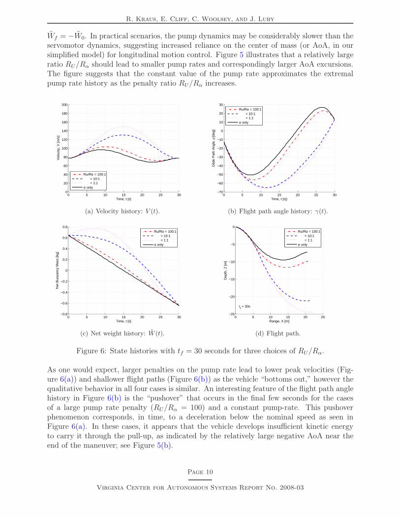
Wf = −W0. In practical scenarios, the pump dynamics may be considerably slower than theservomotor dynamics, suggesting increased reliance on the center of mass (or AoA, in oursimplified model) for longitudinal motion control. Figure 5 illustrates that a relatively largeratio RU/Rα should lead to smaller pump rates and correspondingly larger AoA excursions.The figure suggests that the constant value of the pump rate approximates the extremalpump rate history as the penalty ratio RU/Rα increases.

0 5 10 15 20 25 300

20

40

60

80

100

120

140

160

180

200

Time, t [s]

Vel

ocity

, V [m

/s]

Ru/Rα = 100:1 = 10:1 = 1:1α only

(a) Velocity history: V (t).

0 5 10 15 20 25 30−70

−60

−50

−40

−30

−20

−10

0

10

20

30

Time, t [s])

Glid

e P

ath

Ang

le, γ

[deg

]

Ru/Rα = 100:1 = 10:1 = 1:1α only

(b) Flight path angle history: γ(t).

0 5 10 15 20 25 30−0.8

−0.6

−0.4

−0.2

0

0.2

0.4

0.6

0.8

Time, t [s]

Net

Buo

yanc

y M

ass

[kg]

Ru/Rα = 100:1 = 10:1 = 1:1α only

(c) Net weight history: W (t).

0 5 10 15 20 25−25

−20

−15

−10

−5

0

Range, X [m]

Dep

th, Z

[m]

tf = 30s

Ru/Rα = 100:1 = 10:1 = 1:1α only

(d) Flight path.

Figure 6: State histories with tf = 30 seconds for three choices of RU/Rα.

As one would expect, larger penalties on the pump rate lead to lower peak velocities (Fig-ure 6(a)) and shallower flight paths (Figure 6(b)) as the vehicle “bottoms out,” however thequalitative behavior in all four cases is similar. An interesting feature of the flight path anglehistory in Figure 6(b) is the “pushover” that occurs in the final few seconds for the casesof a large pump rate penalty (RU/Rα = 100) and a constant pump-rate. This pushoverphenomenon corresponds, in time, to a deceleration below the nominal speed as seen inFigure 6(a). In these cases, it appears that the vehicle develops insufficient kinetic energyto carry it through the pull-up, as indicated by the relatively large negative AoA near theend of the maneuver; see Figure 5(b).

Page 10



4.4 Alternative Solution Methods

In addition to using Pontryagin’s Minimum Principle to set up and solve a TPBVP, twomore numerical methods were used for comparison. First, a POST1-like code was used.The second method used DIDO [10]–a commercially available add-in for Matlab that usespseudospectral approximation theory [11] to numerically calculate a solution.

POST-like Solution Method. Our POST implementation imposes a user-specified gridon the time-axis, including nodes at the beginning and the end times. Within each panel thevalue of the control is constant; the collection of control values are unknowns in a NonlinearProgramming (NLP) formulation. The states are propagated over each panel by solving aninitial-value problem (Matlab’s ode45), while fmincon from the Optimization Toolbox

is used to (iteratively) solve the NLP problem. Jacobians are not required but can be suppliedby the user. In this application they were included and improved convergence.

DIDO Solution Method. Similar to the POST-like method, DIDO uses a numericalapproximation based at nodes, but spaces them according to a Legendre-Gauss-Lobatoscheme. The NLP unknowns in the DIDO formulation include both controls and states.The dynamics are approximated by a collocation procedure; the resulting algebraic equa-tions are equality constraints in the NLP problem which is solved via the SNOPT soft-ware http://www.sbsi-sol-optimize.com/asp/sol product snopt.htm. The Jacobiansare computed by finite-differencing; they cannot be supplied by the user.

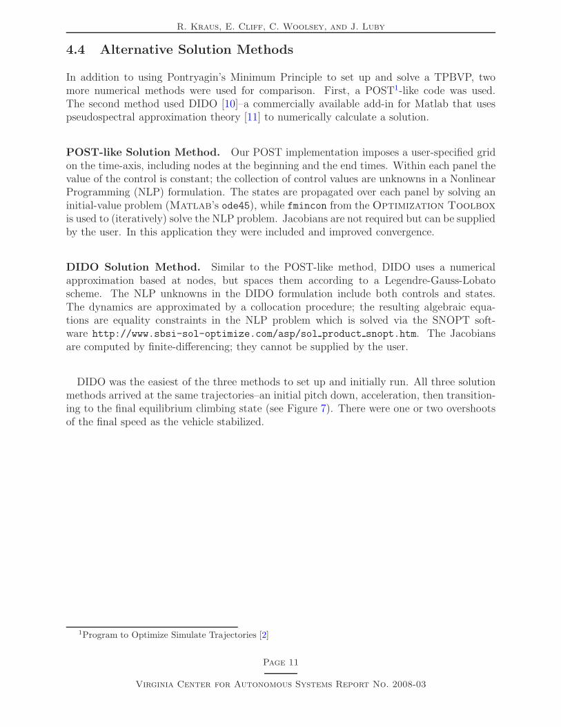
DIDO was the easiest of the three methods to set up and initially run. All three solutionmethods arrived at the same trajectories–an initial pitch down, acceleration, then transition-ing to the final equilibrium climbing state (see Figure 7). There were one or two overshootsof the final speed as the vehicle stabilized.

1Program to Optimize Simulate Trajectories [2]

Page 11



0 10 20 30 40 50 6060

70

80

90

100

110

120

Time, t [sec]

Vel

ocity

, V [c

m/s

]

0 10 20 30 40 50 60−80

−60

−40

−20

0

20

40

60

Time, t [sec]

Glid

e P

ath

Ang

le, γ

[deg

]

0 10 20 30 40 50 60−0.8

−0.6

−0.4

−0.2

0

0.2

0.4

0.6

0.8

Time, t [sec]

Net

Mas

s, ~

m [k

g]

0 10 20 30 40 50 60−6

−5

−4

−3

−2

−1

0

1

2

Time, t [sec]

Ang

le o

f Atta

ck C

ontr

ol, α

[deg

]

0 10 20 30 40 50 60−80

−60

−40

−20

0

20

40

60

Time, t [sec]

Pitc

h A

ngle

, θ [d

eg]

POSTFSOLVEDIDO

Figure 7: Three-state solution method comparison.

5 Longitudinal Dynamics: Rigid Body Model

The model was changed to include three more state variables and to make the rate ofchange of the longitudinal center of mass position the control, rather than AoA. The rate ofchange of the net mass (buoyancy pump rate) was constant. The new equations of motionare:

V = V q sinα cosα

(mu

mw

−mw

mu

)−W

mu

cosα sin θ +W

mw

sinα cos θ

−D

(cos2 α

mu

+sin2 α

mw

)+ L cosα sinα

(1

mu

−1

mw

)

α = q

(mw

mu

sin2 α +mu

mw

cos2 α

)+W

V

(sinα sin θ

mu

+cosα cos θ

mw

)

+D

Vcosα sinα

(1

mu

−1

mw

)−

L

V

(sin2 α

mu

+cos2 α

mw

)

θ = q

q =1

Iyy

((mw −mu)V

2 sinα cosα + Mαα + Mqq −mV g(Xcm cos θ + Zcm sin θ))

˙W = −2W0/tf

Xcm = UXcm

Page 12



Table 1: Initial and final equilibrium states.Initial Conditions Final Conditions

V0 = 77 cm/s V1 = 77 cm/sα0 = 4.3◦ α1 = −4.3◦

θ0 = −8.4◦ θ1 = 8.4◦

q0 = 0 deg/s q1 = 0 deg/s

W0 = 6.18 N W1 = −6.18 NXcm,0 = 1.3 cm Xcm,1 = −1.3 cm

This model includes the added mass terms in the translation and pitch dynamics. It stillassumes the process of moving the center of mass is small and slow enough to not affect theoverall momenta.

Parameters The Lift and Drag profiles are as defined earlier. The pitch Moment profileis described by two terms:

Mα = CMαqSc Mq = CMq

qSc

CMα= −0.15 CMq

= −10.0

where

c = 0.1311 m

Iyy = 13.177 kg · m2

The vertical position of the center of mass was fixed at Zcm = 5 cm below the centerline.The combined initial and final (equilibrium) conditions were prescribed as shown in Table 1.

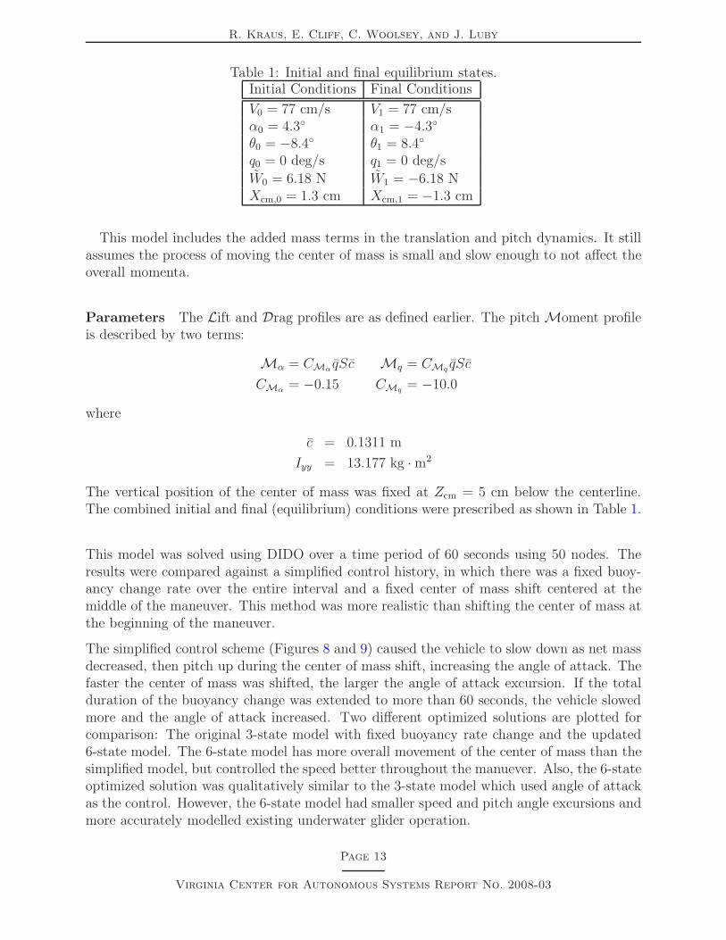
This model was solved using DIDO over a time period of 60 seconds using 50 nodes. Theresults were compared against a simplified control history, in which there was a fixed buoy-ancy change rate over the entire interval and a fixed center of mass shift centered at themiddle of the maneuver. This method was more realistic than shifting the center of mass atthe beginning of the maneuver.

The simplified control scheme (Figures 8 and 9) caused the vehicle to slow down as net massdecreased, then pitch up during the center of mass shift, increasing the angle of attack. Thefaster the center of mass was shifted, the larger the angle of attack excursion. If the totalduration of the buoyancy change was extended to more than 60 seconds, the vehicle slowedmore and the angle of attack increased. Two different optimized solutions are plotted forcomparison: The original 3-state model with fixed buoyancy rate change and the updated6-state model. The 6-state model has more overall movement of the center of mass than thesimplified model, but controlled the speed better throughout the manuever. Also, the 6-stateoptimized solution was qualitatively similar to the 3-state model which used angle of attackas the control. However, the 6-state model had smaller speed and pitch angle excursions andmore accurately modelled existing underwater glider operation.

Page 13



0 10 20 30 40 50 6040

50

60

70

80

90

100

110

120

Time, t [sec]

Vel

ocity

, V [c

m/s

]

0 10 20 30 40 50 60

−10

−5

0

5

10

Time, t [sec]

Ang

le o

f Atta

ck C

ontr

ol, α

[deg

]

0 10 20 30 40 50 60−60

−40

−20

0

20

40

Time, t [sec]

Pitc

h A

ngle

, θ [d

eg]

0 10 20 30 40 50 60−60

−40

−20

0

20

40

Time, t [sec]

Glid

e P

ath

Ang

le, γ

[deg

]

0 10 20 30 40 50 60−4

−2

0

2

4

6

Time, t [sec]

Long

itudi

nal c

g lo

catio

n, X

cg [c

m]

0 10 20 30 40 50 60−0.8

−0.6

−0.4

−0.2

0

0.2

0.4

0.6

0.8

Time, t [sec]

Net

Mas

s, ~

m [k

g]

Fixed cg shift rateControlled Shift RateControlled α

Figure 8: Fixed rate model comparison with optimized models.

0 5 10 15 20 25 30 35

−20

−15

−10

−5

0

X−Position, X [m]

Z−

Pos

ition

(D

epth

), Z

[m]

Trajectory

Fixed cm Shift at Halftime3−State: Fixed Buoyancy Rate6−State Rigid Body

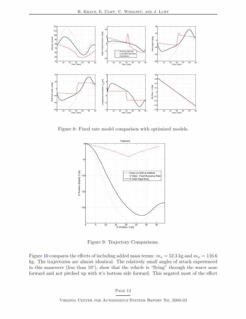
Figure 9: Trajectory Comparisons.

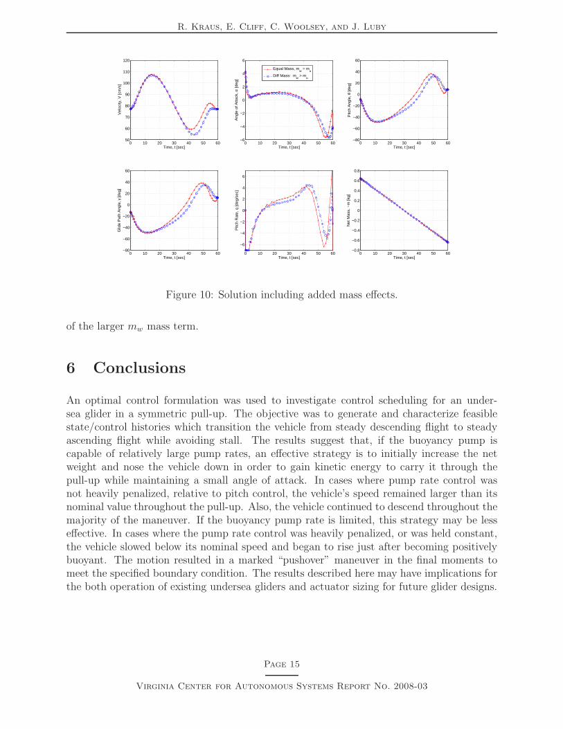
Figure 10 compares the effects of including added mass terms: mu = 52.3 kg and mw = 116.6kg. The trajectories are almost identical. The relatively small angles of attack experiencedin this maneuver (less than 10◦), show that the vehicle is “flying” through the water noseforward and not pitched up with it’s bottom side forward. This negated most of the effect

Page 14



0 10 20 30 40 50 6050

60

70

80

90

100

110

120

Time, t [sec]

Vel

ocity

, V [c

m/s

]

0 10 20 30 40 50 60−6

−4

−2

0

2

4

6

Time, t [sec]

Ang

le o

f Atta

ck, α

[deg

]

0 10 20 30 40 50 60−80

−60

−40

−20

0

20

40

60

Time, t [sec]

Pitc

h A

ngle

, θ [d

eg]

0 10 20 30 40 50 60−80

−60

−40

−20

0

20

40

60

Time, t [sec]

Glid

e P

ath

Ang

le, γ

[deg

]

0 10 20 30 40 50 60

−6

−4

−2

0

2

4

6

Time, t [sec]

Pitc

h R

ate,

q [d

eg/s

ec]

0 10 20 30 40 50 60−0.8

−0.6

−0.4

−0.2

0

0.2

0.4

0.6

0.8

Time, t [sec]

Net

Mas

s, ~

m [k

g]

Equal Mass, mw

= mu

Diff Mass: mw

> mu

Figure 10: Solution including added mass effects.

of the larger mw mass term.

6 Conclusions

An optimal control formulation was used to investigate control scheduling for an under-sea glider in a symmetric pull-up. The objective was to generate and characterize feasiblestate/control histories which transition the vehicle from steady descending flight to steadyascending flight while avoiding stall. The results suggest that, if the buoyancy pump iscapable of relatively large pump rates, an effective strategy is to initially increase the netweight and nose the vehicle down in order to gain kinetic energy to carry it through thepull-up while maintaining a small angle of attack. In cases where pump rate control wasnot heavily penalized, relative to pitch control, the vehicle’s speed remained larger than itsnominal value throughout the pull-up. Also, the vehicle continued to descend throughout themajority of the maneuver. If the buoyancy pump rate is limited, this strategy may be lesseffective. In cases where the pump rate control was heavily penalized, or was held constant,the vehicle slowed below its nominal speed and began to rise just after becoming positivelybuoyant. The motion resulted in a marked “pushover” maneuver in the final moments tomeet the specified boundary condition. The results described here may have implications forthe both operation of existing undersea gliders and actuator sizing for future glider designs.

Page 15



Acknowledgements. The authors are grateful to Nina Mahmoudian for her input con-cerning glider steady motions. This work was sponsored, in part, by AFOSR under Grant#FA9550-07-1-0273 and by ONR under Grant #N00014-08-1-0012.

Page 16



References

[1] P. Bhatta. Nonlinear Stability and Control of Gliding Vehicles. PhD thesis, PrincetonUniversity, 2006.

[2] G.L. Brauer, D.E. Cornick, and R. Stevenson. Capabilities and applications of theprogram to optimize simulated trajectories. Technical Report NASA CR-2770, MartinMarietta Corporation, 1977.

[3] C. C. Eriksen, T. J. Osse, R. D. Light, T. Wen, T. W. Lehman, P. L. Sabin, J. W.Ballard, and A. M. Chiodi. Seaglider: A long-range autonomous underwater vehicle foroceanographic research. Journal of Oceanic Engineering, 26(4):424–436, 2001. SpecialIssue on Autonomous Ocean-Sampling Networks.

[4] A. M. Galea. Optimal path planning and high level control of an autonomous glidingunderwater vehicle. Master’s thesis, Massachusetts Institute of Technology, 1999.

[5] J. G. Graver. Underwater Gliders: Dynamics, Control, and Design. PhD thesis, Prince-ton University, 2005.

[6] S. A. Jenkins, D. E. Humphreys, J. Sherman, J. Osse, C. Jones, N. Leonard, J. Graver,R. Bachmayer, T. Clem, P. Carroll, P. Davis, J. Berry, P. Worley, and J. Wasyl. Under-water glider system study. Technical Report 53, Scripps Institution of Oceanography,May 2003.

[7] R. Kraus, E. Cliff, C. Woolsey, and J. Luby. Optimal control of an undersea glider in asymmetric pull-up. In Proceedings of the 18th International Symposium on MthermaticalTheory of Networks and Systems, Blacksburg, Virginia, 2008.

[8] N. Mahmoudian, J. Geisbert, and C. A. Woolsey. Steady turns and optimal paths forunderwater gliders. In AIAA Guidance, Navigation, and Control Conference, HiltonHead Island, SC, August 2007. AIAA-2007-6602.

[9] L. S. Pontryagin, V.G. Boltyanskii, R. V. Gamkrelidze, and E. F. Mishchenko. TheMathematical Theory of Optimal Processes. Wiley-Interscience, 1962.

[10] I. Michael Ross. A Beginner’s Guide to DIDO (Ver 7.3): A MATLAB Applicationpackage for Solving Optimal Control Problems. Elissar, LLC, Monterey, CA, 2007.

[11] I.M. Ross and F. Fahroo. Legendre pseudospectral approximations of optimal con-trol problems. In Lecture Notes in Control and Information Sciences, pages 327–342.Springer-Verlag, New York, NY, 2003.

[12] J. Sherman, R. E. Davis, W. B. Owens, and J. Valdes. The autonomous underwaterglider “Spray”. Journal of Oceanic Engineering, 26(4):437–446, 2001. Special Issue onAutonomous Ocean-Sampling Networks.

Page 17



[13] D. C. Webb, P. J. Simonetti, and C. P. Jones. SLOCUM: An underwater glider propelledby environmental energy. Journal of Oceanic Engineering, 26(4):447–452, 2001. SpecialIssue on Autonomous Ocean-Sampling Networks.

Page 18


r. kraus, e. cliﬀ, c. woolsey, and j. luby · 2009-06-02 · r. kraus, e. cliff, c. woolsey, and...

Documents