RlSK ANAlYSlS TECHNIQUES IN DEFENCE PROCUREMENT

Keith Hull MSc CEng MIEE

This paper explains the risk analysis techniques u e d by the Accountancy, Estimating and Pricing Services (AEPS). Ministry o f Defence. Procurement Executive. The aim of the paper is to provide a convenient reference document for procurement staff rather than to advance &he theory. Topics covered include identification of risk mens. approaches to risk analysis and strategies for risk reduction and control.

The choice o f risk analysis technique depends on the definition. scale and phase o f the project. All techniques, howewr. require a systematic approach. so a generaiised methodology for risk analysis is proposed. Whilst risk analysis methods and models are valuable tools. the right answers still depend upon judgement and specialist expertise.

INTRODUCTION.

Risk is a part of everyday life and is usually associated with advene or harmful events, but individuals do have a degree of choice in the levels of risk to which they are prepared to expose themselves. Managers have a similar choice when managing the risks within their particular projects.

There is a need to identify risks especially during the early stages of a project, and to implement an effective risk management plan to ensure that risks are reduced to an acceptable level as the project proceeds. Not doing so may result in failing to meet performance requirements and/or serious cost and schedule overruns. A properly implemented approach to risk management will allow managers to conc- entmte ~ S O U I - C Z S into those ares where risksare perceived Y being high and to conuin risks within reasonable and acceptable limits. The assessment of risk and its management is a continuous process. It is therefore necessary that risk assessments are

made at the s t a r t of the project and when options are being compared. Hence, risk management should be integrated into the overall project management process and performed continuously.

Engineers and Accountmu of AEPS have applied risk assessment techniques of varying degrees of complexity for many yeus, but have used more formal approaches since 198 1. Before explaining our approach, the need for and benefits of risk analysis will be discussed. Some definitions will then be given. The approach we have adopted is presented and the idea of a risk management process is explored. Finally, we describe the current methods and models used by AEPS.

The need for risk analysis.

There is, of course, nothing new about risk analysis. The basic theory has been around for a long time. However, there has been little demand for these techniques in an environment where risks can be diluted by distributing them over many contracts/projects and where risks CM be passed on. With competition and incentive pricing t h e n is now a more open market for defence work, and much of the burden of risk and responsibility is being transferred from MOD to industry. Not all risks can or should be transferred. Some risks will not be cost effective to push onto the contractor and others may not be fully accepted and may rebound back onto MOD if the risks materialhe. It is, therefore, 'Important for both industry and MOD to identify and evaluate risk, particularly when projects involve significant new technology and long timescdes. The House of Commons Defence Committed found that the roots of cost escalation, and in some cases project cancellation, were due to an insufficiently critical approach to technological risk assessment. This was coupled with an unjustified optimism in the ability Of contrac:ors to develop solutions dependent upon

'House of Commons Defenca Committer Fifth Rzport Session 1987-88.

3/1

-

unproven technology, within the price tendered and time constraints of the project. MOD cannot be fully protected from the consequences of the failure of its contractors simply by adoption of new contracting initiatives. Incentive contracts place an even greater importance on the need for tightly drawn specifications and statements of work based on proper risk assessment.

Project Managers run the risk of their projects failing in one or more of the following ways;-

1. Performance not up to specification. 2. Poor Reliability and Maintainability. 3. Late delivery. 4. Cost too high.

Such risk indicators are to acertain extent inter-related in that compromises made in one element may have consequential effects on the others.

A B

Figure 1. Single Point Estimate.

Conventionally, performance, cost and schedule estimates are deterministic; that is, the estimates are expressed as single values. Figure 1, illustrates the situation where only single point estimates are given for two proposais. Uncertainty is not measured, they contain no measure of quality and they belie the existence of a range of possible outturns. With this information the decision maker may well choose "A" as the best proposal, if the estimates relate to delivery timescales for example. However if uncertainty in the estimates are taken into account his decision may well be different. Figure 2, shows the case when the estimates are expressed as probability distributions to reflect the uncertainty surrounding the outturns of each proposal. The situation depicted is that there is some probability that the outturn of "A" will be higher than "B. If this probability is small, the decision maker would still select "A". However, when the overlap is significant, the single-value estimates would no longer provide a valid criteria for selection.

A B

Figure 2. Estimates with Uncertainty

The benefits of risk analysis.

Risk analysis has been used in AEPS primarily for fixed/firm price contract estimating. The use of risk analysis has a number of benefits. It allows accountants and engineers to take account of the degree of variation within individual elements of estimates and makes it more difficult for a supplier to exaggerate the need for blanket contingencies. It provides an indication of the reliability of the estimates and enables sensitivity testing of the various performance, reliability, maintainability, cost and schedule components. It can also provide contract negotiators and tender evaluation panels with a quantified assessment of risk for particular pricing situations and gives project management better insight, knowledge and confidence for decision making and risk management. Better informed decision makers are able to control risk rather than be controlled by it. Of these benefits, it is the ability to provide advice on the level of confidence we have in our estimates which provided AEPS management with the initial justification for undertaking risk analysis. It has applications in most areas (including Capital Investment Programmes and Long Term Costings) where judgements involving risk need to be made or assessed.

Definitions.

The reminder of this section defines and make some distinctions between risk and uncertainty, risk assessment and risk management, objective and subjective probabilities, endogenous and exogeneous risk variables, and, in the context of proposal and investment appraisals, estimation bias and variability risk.

Risk and Uncertaintv.

Risk can be described as the product of the probability of an event occurring and its consequences or, in other words, risk is about uncertainty and its impact. Uncertainty alone puts no one at risk, it is the resulting impact of

the event that is important. Thus attention is best concentrated on those events or activities where the magnitude of the consequences or impact of an adverse event occurring is significant. These consequences would manifest themselves as financial loss, time delay or under achievement of performance. Therefore the risk analysis must cover both the probability of occurrence and the impact of adverse events.

Analvsis and Risk

Risk Analysis is the assessment of uncertainty and impact with a view to understanding the associated implications in order to manage, reduce, transfer or control risk. Risk Analysis tells us the probability of the performance meeting the requirement or of having a cost or schedule overrun, it indicates the amount of the shortfall in performance or how large the overrun can be. Risk Management refers to the sum total of all the processes used in the management of risk. Its aim is to identify, analyse, reduce and control risk. It also involves the development of suitable strategies and fall back options to minimise the impact of uncertainty.

. . . . ...

Objective probabilities arc where the relative frequency of evenrs can be measured, for example, tossing coins or rolling dice. However, much of the information necessary to produce probabilities in risk analysis involves interpretation and adjustment of objective data, or judgements based on experience with no directly relevant data. This information is therefore subjective, and could be highly unreliable. As it is the aim of risk analysis to create the basis upon which effective decisions are made, it is important that subjective probabilities of outcomes arc as reliable as possible, and that the sources of unreliability are well understood.

eous R i s k

Endogenous risks are, to some extent, under the control of the project managers. Exogeneous risks, on the other hand, refer to risks like exchange rate, suppliers going bankrupt, flooding, fire and 'Acts of God' which are normally beyond the control of those managing projects.

variation around the mathematical expected value of an outcome. The majority of the literature on risk assessment is concerned with this risk.

Estimation bias is one of the main sources of data unreliability and can be reduced by critical scrutiny of the estimates, using independent expert advice as necessary to help decide whether individual figures are reasonable.

RISK ANALYSIS APPROACH.

The approach we have adopted in AEPS is to combine risk aaalysis with the normal pricing activity. Cost and schedule estimating must, among many other things, take into account the levels of technical performance of the equipment required, the resources to be used and timescalea to be achieved. Combining risk analysis and the pricing process has some major benefits. A direct measure of risk is obtained at the same time as the estimate is formed and therefore allows the contingency value, if required, to be quantified. Insight into risk is achieved by using methods which enable sources of risk to be identified and examined in a systematic manner. This also gives a better understanding of the correlation (interdependencies) between items, which can have large combined effects on the overall distribution.

The level of detail required for the risk assessment should be that warranted by the value and perceived uncertainty as well as the time constraints on the task. Generally speaking, the lower the perceived risk (which is dependent on definition, phase, size and complexity), the simpler the exercise required.

To implement our strategy we have produced computational models and methods that can be used easily and quickly by AEPS accountants and engineers in the field. Field officers have been trained in the use of risk analysis and have the support, when required, of a team of analysts in the Estimating Techniques Group.

RISK MANAGEMENT METHOD.

. . . . Risk management techniques require a systematic approach designed to suit the model

It is sometimes useful to divide risk into and the circumstances in which they are used. two types: estimation bias and variability risk. The method described here is a fairly detailed Estimation bias refers to the systematic error or and general one which consists of four distinct tendency to overestimate or underestimate. phases, namely the risk identification, analysis, Variability risk measures the degree of expected

3 /3

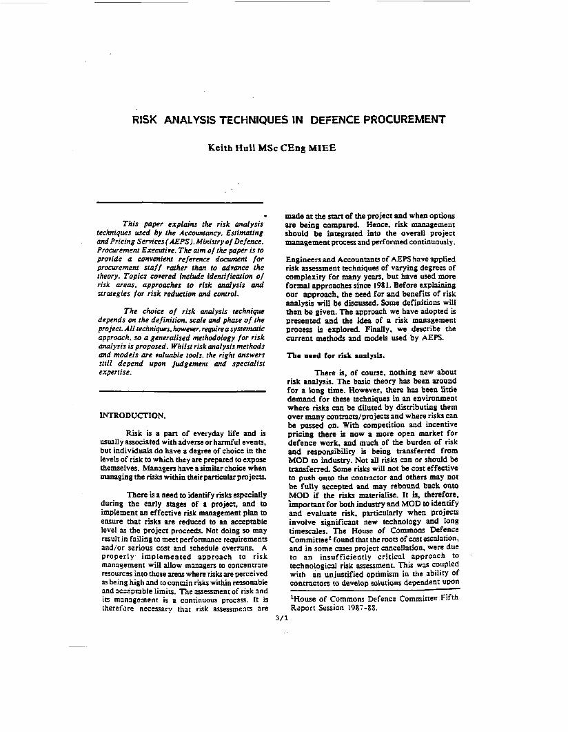
planning and management stages shown in Figure 3.

Figure 3. The Risk Management Process.

Briefly. the identification phase is qualitative and involves breaking the task down and identifying the risks and their responses; the analysis phase models the individual elements and then combines them to form an overall resulc the planning and management phases involve planning and taking the corrective action either to eliminate or lesson risks. Each phase is divided into a number of steps. A similar approach was first described by Chapman and Cooperfl].

Risk Identification Phase

The aim of the Identification Phase is to gain a clear understanding of the task in hand and to discover what risks are involved and the possible responses that could be made if these risks materialised.

Step 1 Identification of Key Parameters.

Familiarise with all relevant and available information including the contractor proposals with supporting data, Invitation T o Tender (ITT), Requi rement Specification, management plans and past similar projects. Identify the objectives, define contract/system boundaries, external interfaces and sub- contract/sub-system interdependencies. List main requirements, equipment to be procured, critical milestones etc.

Step 2 Decomposition of Task into Key Elements or Activities.

Divide the task into meaningful elements or activities and define their interactions. This step provides the necessary work breakdown structure required for assessment and can be based on the list of requirements, Contractor’s proposal or quotation line items. Activities having a large impact should be decomposed further. Items with a relatively small

3/4

impact and where risks are similar should be consolidated. Activities for the integration of sub-systems and the total system must not be overlooked.

Step 3 Define Each Activity.

Describe in detail each activity. This helps to define what is involved and what is not. Obviously the time spent on each activity should be in proportion to the value and perceived risks.

Step 4 Identify Sources of Risk.

List and describe all sources of risk for each activity. Evaluate plans for contradictions and voids. Identify the anticipated point at which the risk would be realised if no corrective action were taken. Each main area of uncertainty will have a number of component risks associated with it which may include:

Scientific Risk. Will it actually work? Is the activity specification within the bounds of physical possibility? Are there any inconsistencies in the requirement.

Technological Risk. Does the current state of technology allow the project to be undertaken within asatisfactory level of risk; is the technology proved and in place to bridge the innovation gap? (A lot of projects in the past have produced long delays, major cost overruns and performance shortfalls due to technological difficulties.)

Engineering Risk. What are the risks involved in the engineering processes? Will the necessary resources in terms of plant, labour, tools etc be available to carry out the required activities?

Supply Risk. To what degree is the activity dependent on the supply of goods or services. What material is particularly scarce?

Business Risk. What, if any, are the risks to the project from the Contractor’s decision making and operating situation. Do they have the necessary management team and funding to carry out this project?

Commercial Risk. Is there any risk

that the Contractor may be affected by commercial forces?

Political Risk. Could the project be affected by political decisions and what political events may introduce changes in policy?

International Risk. In the C+C of collaborative projezts extra risks occur ranging from agreeing exchange rates up to the possibility of the withdrawal of a nation.

There are many other potential sources of risk that can impact on a particular project.

Figure 4. shows the project with several risk sources or drivers attacking from all sides.

PERFORYANCE I€-- \ \

Figure 4. Risk Components.

The risks impact on the project and affect performance, reliability, maintainability, schedule and cost. Hence, the aggregated effect of the technical and non-technical risks can be expressed in terms of performance shortfalls, poor reliability, difficult maintainability, schedule delays and cost overruns. Understanding the sources of risk and the impact areas provide a structure or framework to examine risks effectively.

Step 5 Determine Risk Responses.

Examine the sources of risk identified in Step 4 and determine the consequences and necessary responses should these risks materialise. If any of the Responses also contain significant risks these must also be considered. Search for common- mode and cascade relationships. Exclude from further consideration those risks which involve a negligible probability or effect on the final result.

Step 6 Identify Dependent Risks

more than one activity. These activities should be factored to remove the dependent component or grouped together in correlation pairs or dependency groups.

RIsk Analysis Phase

The Analysis Phase assesses the impact of the risks identified and provides information on the risks to be targeted during the planning and management phases. This is normally achieved by a qualitative and quantitative analysis. If the availability or quality of data make quantification impossible, doing just a qualitative analysis is st i l l worthwhile.

1

w m

m y D w - IMPACT

Figure 5. Risk Impact Diagram/Matrix.

Step I

Step 8

Preparatory Quantification

Before the quantification process starts in earnest it is sometimes a good idea to organise. rank and rate the risks for further evaluation. The impact diagram, figure 5 , offers a conceptual diagram for a risk rating mechanism. It can be used by identifying individual risk by marking them on the matrix to give a quick pictorial view of the main risks.

Estimate Activities.

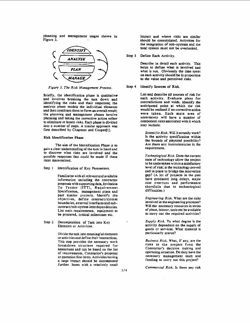
Estimate the range of probabilities and values that can reasonably be anticipated for each activity, using the information obtained in the risk identification phase. This will define the distribution of values for each activity. For example, if an activity can take between 2 - 10 days, breakdown the range into intervals, say 2 days and estimate the probability of each interval, see figure 6.

Identify those risks which are present in

0.4

0.3 2

g 0.2 B

0.1

Figure 6 . Activity Estimaie Example.

Note probabilities must add up to one. To help order events and ensure the relevant axioms of probability are not violated there are schemes, such as the " Modi f i ed Churchman - A c ko f f method".

Alternatively, a probability distribution can be selected from a range of distributions that reflect most accurately the estimator's belief, figure 7. If the estimator believes an activity can take on a number of equally likely values between a minimum and maximum then a uniform distribution is chosen. A triangular distribution can model the circumstances when the estimator feels it is more likely that the values will centre on some figure and reduce towards the limits. The Beta distribution is discussed later.

BL(TocL(y

n

Figure 7 . Distribulions Used in Risk Analysis.

Judgements should be based whenever possible on historical data, relevant experience and advice from others with specialist knowledge. Catastrophic variations, such as major design changes,

Step 9

Step 10

labour problems, floods, etc should be considered outside the scope of the assessment and treated as contract conditions.

Aggregate Activities.

Combine the risk estimates for each activity using manual procedures, simple computer routines, commercial risk analysis software, or in-house computer package.

Estimate Correlation Coefficients Between Activities.

A general difficulty in combining uncertain events is the need to consider probablistic dependence between ac t iv i t ies . T h e combina t ion of independent activities produces results that have less spread than if they were dependent elements. Hence, if activities are assumed to be independent when they are not, an underestimate of the overall risk will result. Accounting for dependence can be achieved by applying one of the following methods:-

a. Determine and apply correlation coefficients to the activities. Without historical data this step could be difficult.

b. Aggregate all elements which are dependent into a single separate independent element.

c. Run the analysis twice. First assume no correlation and then assume total correlation. The correct result will lie between the two.

d. Factor out the common elements.

Step 11 Sensitivity Analysis.

Several iterations or partial iterations of the above approach might be appropriate. Different levels of detail can be tried or values can be changed to discover the sensitivity of any activity.

Step 12 Report.

Report final results and update risk database/log.

Risk Planning Phase

The aim of the Risk Planning Phase is to prepare risk reduction, elimination and fall-back plans for managing the risks that may impact on the project.

RISK ANALYSIS MODELS AND TECHNIQUES.

Step 13 Plan Risk Reduction

Study the results and determine the cost and benefits of the Risk Identification and Analysis process and make necessary plans to remove, reduce or transfer risks. This is done by changing the existing project plans, specificatiops, chosing different alternatives and sharing the risks with others. Fallback Plans, Le., plans which are implemented after the risk occurs or at some trigger event, should be developed for residual or accepted risks.

Risk Management Phase

The objective of the Risk Management Phase is to implement the mechanisms and plans to reduce risk. By making comparisons between the current and previous Risk Analysis results appropriate management decisions may be taken. This phase also includes monitoring, controlling and reporting.

Step 14 Manage Risks

Install and maintain monitoring procedures to provide updates to the Risk Analysis. Decide and implement the corrective actions to be taken in order to achieve required cost, timescale, re l iab i l i ty , main ta inabi l i ty and performance goals.

The method outlined is quite a detailed approach and if applied rigourously can be expensive in manpower. Clearly, not all tasks justify such a detailed approach and must be tailored to suit the task.

*Programme Evaluation and Review Technique (PERT). SGraphical Evaluation and Review Technique (GERT). 'Venture Evaluation and Review Technique (VERT).

3/7

The models used for the analysis phase range from simple procedures and adjustments for the addition of independent activities to more complex techniques including probability trees, activity networks (PERTZ, GERTS and VERT') and simulation.

The choice of risk technique depends on the level of definition of the project, its value, perceived uncertainty and many other factors.

This section looks briefly at some of the main models and techniques used for risk analysis.

Payback Period.

Decision criteria such as the payback period of the project, its accounting rate of return, the Net Present Value (NPV) and the Internal Rate of Return (IRR) are often used in financial investment appraisals to judge a project's worth or risk.

The payback period is the time needed for the total (discounted or undiscounted) benefits to equal the s u m of costs. In other words the payback period is the time needed to recover the capital investment and the time for which the capital is "at risk".

Payback adopts a very simplistic approach to risk and can be a poor decision criteria for investment appraisals as it treats all benefits and costs as certain and ignores them completely after the break even point. Nevertheless, this crude indicator is widely used, probably due to the ease with which it can be calculated and understood. It can sometimes be useful as a supplement to other risk techniques particularly if used in conjunction with a measure of the project's overall Net Present Value (NF'V). NPV is calculated as follows:-

U

where B; are the net benefits and ris the discount rate. Some analysts use an internal rate of return (IRR) which will give almost the same ranking of projects as the payback period. IRR is that discount rate for which NPV = 0. The most common decision criterion is that the investment is worthwhile if the NPV is positive using a discount rate defined by the next-best use Of

.-

BASIC ESTIMATE fM

RADAR DEVELOPMENT COSTS

RISK FACTOR REVISED ESTIMATE fM

WBS ELEMENT

AERIAL TRANSMITER

Sig Gen Amp

RECEIVER POWER SUPPLY PROCESSOR DISPLAY SYSTEM ITEGRATION

TOTAL

9

20 15 22

5 25 4 . 2

1.20

1.30 1.35 1.20 1.20 1.40 1.04 1.60

11

26 20 26 6

35 4 3

I 102 131 I Table I Example Using Risk Factors.

capital, or if IRR exceeds the return from the next-best use of capital.

Adjustment of the discount rate is sometimes used as a way of allowing for risk. For example, a larger discount rate might be used in the IWV calculation, or the IRR might be required to exceed the return from a relatively risk-free investment by some “risk margin”. However, this kind of adjustment does not assess the degree of risk involved and gives no indication of whether the safety margin is appropriate. Besides being crude, it pushes decisions in favour of options with short term high risk rather than long term comparatively safe ones.

Risk Factors.

The Risk Factor method estimates the total added cost or time that might be expected due to risks. Risk Factors are multipliers which are used to increase individual project elements (basic estimate) according to the perceived risks. Table 1 illustrates the technique.

The baseline project estimate of f 102M has been revised to f 13 1M to accommodate additional costs that may result from risks. Analysis of past projects and discussions with knowledgeable engineers and managers can assist in determining the factors that should be applied. It is important to know what is in the “basic estimate’’ because often these estimates do contain allowances and are not necessarily minimum/best estimates.

Sensitivity Analysis.

Sensitivity analysis shows how changes in the values of various factors affect the final project out-turn. Alternatively, sensitivity analysis can determine the bounds on specific parameters for which the out-turn is still acceptable, with a l l other parameters set to their nominal, pessimistic, optimistic or expected values. This enables the most important parameters to be identified for further analysis and monitoring.

It is important that only plausible ranges of values are chosen for uncertain parameters. The ranges will not in general be the same or symmetric for all variables. Also, the relationships or correlations between factors must be carefully considered. Correlated parameters are best identified by looking a t the underlying sources of risk as explained earlier.

Comprehensive sensitivity analysis can give the analyst a good feel for the overall risk of a project or a particular decision. Projects for ,which the out-turn figure varies greatly as a result of small changes in certain key variables are clearly very risky. Conversely, if the out-turn is virtually invariant to the largest plausible changes in all variables then the project can be considered low risk.

Given its simplicity and wide range of uses, it is not surprising that sensitivity analysis is the most popular risk appraisal technique.

3 / 8

A

B

c

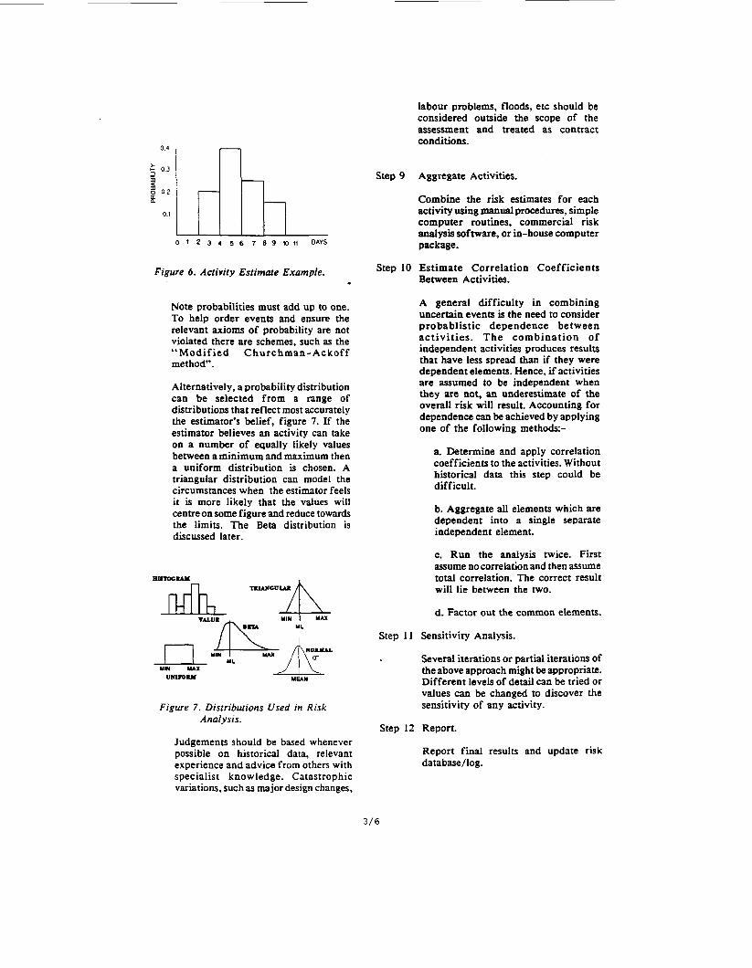
Table 2 Caldation of the Expected Value ( E ) and Standard Deviation.

PS 5 4x1 UX& (E(.>-+ mxF@P,

0.5 100 50 4 5 9025 45 12.5 0.5 4) 4 95 9025 45 12.5

4 x 1 = 5 VAR= 9025 m= 95 cv = 19

0.5 10 5 -5 25 12.5 0.5 0 0 5 25 12.5

WX) = 5 VAR= 25 m= 5 cv- 1

0.5 100 50 -50 2500 1250 0.5 0 0 50 wlo 1250

Yx)= M vAR= 2500 50

cv = 1

Expected Values and Measures of Spread.

The "expected" outcome is the sum of all possible outcomes where each outcome is weighted by its probability. It is simply the average or mean outcome. For example, suppose a contractor has a contract or activity which makes a large number of items and each item has an uncertain cost out-turn as follows:-

0.3

Expected cost = f5000x0.1 +f 10000~0.6 +f15OOOxO.3

=f 11000 The expected cost for each item is

f 1 1.000 and providing the contractor sets the price above this value a profit will be made in the long run. Although the expected value does describe the probability distribution in the long term it is of limited applicability when there are few, or no replications. If the cost profile in the example was estimated for a particular event then setting the price based on the expected cost may well be unfair as the chance of over charging is

very high (greater than 0.7 in this case).

The spread of possible outcomes is, of course, an indication of the amount of risk involved in a project, This spread is normally measured using the standard deviation given by-

where E(x) is the expected value, xs denotes the outcome and Ps the probability.

The calculation of the standard deviation and its interpretation is illustrated by the following example:

A has a 0.5 chance of achieving an NPV of f 100 and a 0.5 chance of -f90.

B has a 0.5 chance of achieving an NPV of f10 and a 0.5 chance of fO.

C has a 0.5 chance of achieving an NPV of flOO and a 0.5 chance of fO.

In both A & B the Expected NPVs are f S

3/9

but the spread around this value is much greater for A (=f95) than B (=f5),dee Table 2. Where options have the same expected value the greater the standard deviation the options have, the more risky they are. So A is more risky than B, which accords with intuition.

Option C has an expected NPV and a standard deviation of f5O. However, the standard deviation is a poor measure of risk when comparing projects or activities which have different m e g valueL In this case the Coefficient of Variation (standard deviation divided by the expected value) is more appropriate as this measures the riskiness per unit of cost, time or benefit. Options A, B & C have coefficient of variances of 19, 1, and 1, respectively. On this measure C has less risk per unit of benefit than A and the same as B, which also accords with intuition.

Method of Moments

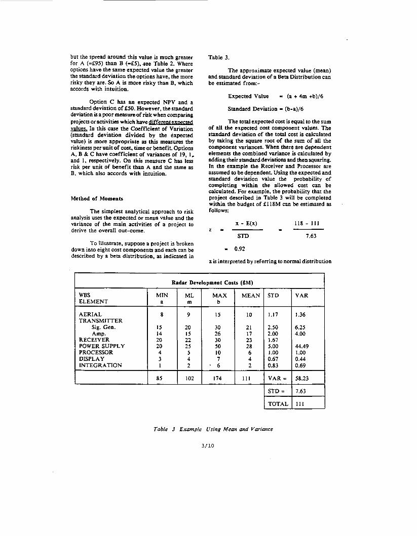
The simplest analytical approach to risk analysis uses the expected or mean value and the variance of the main activities of a project to derive the overall out-come.

To illustrate, suppose a project is broken down into eight cost components and each can be described by a beta distribution, as indicated in

Table 3.

The approximate expected value (mean) and standard deviation of a Beta Distribution can be estimated from-

Expected Value = (a + 4m +b)/6

Standard Deviation = (b-a)/6

The total expected cost is equal to the sum of all the expected cost component values. The standard deviation of the total cost is calculated by taking the square root of the sum of all the component variances. When there are dependent elements the combined variance is calculated by adding their standard deviations and then squaring. In the example the Receiver and Processor are assumed to be dependent. Using the expected and standard deviation value the probability of completing within the allowed cost can be calculated. For example, the probability that the project described in Table 3 will be completed within the budget of f 1 ISM can be estimated as follows:

118 - 111 x - E(x) z = I

STD 7.63

= 0.92

z is interpreted by referring to normal distribution

WBS ELEMENT

AERIAL TRANSM-R

Sig. Gen. Amp.

RECEIVER POWER SUPPLY PROCESSOR DISPLAY INTEGRATION

Radar Development Costs (fM)

MIN 1 ”,” I M t X 1 MEAN a

5.00 44.49 1 .oo 0.67 0.44 0.83

1 STD- 176; 1 TOTAL 1 1 1

Table 3 Example Using Mean and Variance

3/10

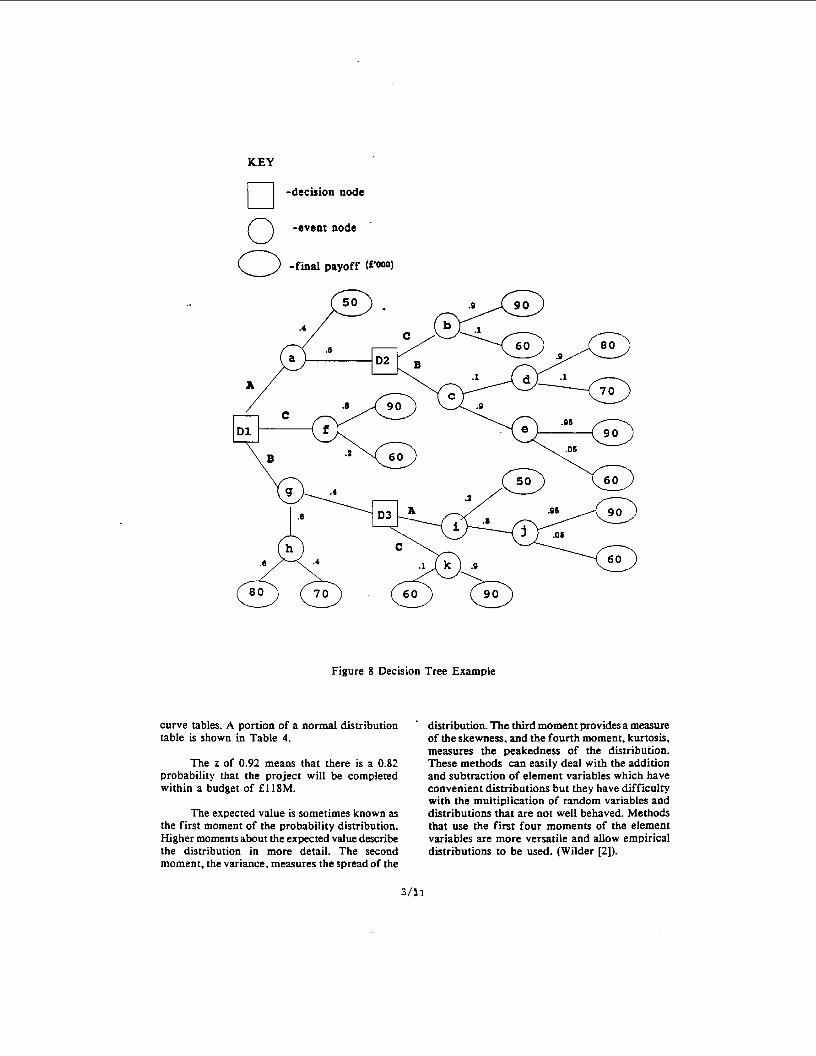
KEY u -decision node

-event node 0 0 - f ind payoff (f*om)

Figure 8 Decision Tree Example

curve tables. A portion of a normal distribution table is shown in Table 4.

The L of 0.92 means that there is a 0.82 probability that the project will be completed within a budget of f 1 18M.

The expected value is sometimes known as the first moment of the probability distribution. Higher moments about the expected value describe the distribution in more detail. The second moment, the variance, measures the spread of the

distribution. The third moment provides a measure of the skewness, and the fourth moment, kurtosis, measures the peakedness of the distribution. These methods can easily deal with the addition and subtraction of element variables which have convenient distributions but they have difficulty with the multiplication of random variables and distributions that are not well behaved. Methods that use the first four moments of the element variables are more versatile and allow empirical distributions to be used. (Wilder [Z]).

3/11

Table 4 Cumulative Proportions of Area under the Normal Curve for selected values of 2

Z

-3 -2 -1 0 .92 1 2 3

Probability

0.00 13 0.0228 0.1587 0.5000 0.8210 0.84 13 0.9772 0.9987

choose one of three Options A, B, & C. Option A is the cheapest at f50K but may not be available. Option B is f8OK but there is a chance that a f 10K discount can be obtained, however, it too may not be available. Option C, on the other hand, is certain to be available and has a price of f90K with a chance of a f30K discount. Figure 8 below shows the decision tree for the option selection problem.

The tree is drawn from left to right on the basis of the known information about costs, discounts and probabilities. The probabilities for availabilities and discounts become less favourable with time. For example, it is known that the probability of obtaining Option A is 0.4 while at the later event node i it is 0.2.

Monte Carlo Simulation.

When there are a large number of activities or element variables to be combined, or where there are complex dependence relationships between variables it is often too difficult to do the job analytically. In these cases analysts usually turn to computer sampling techniques such as Monte Carlo Simulation. This requires descriptions of the probability distributions for each element and a description of any interrelationships between these distributions. Using this knowledge, the computer takes one random drawing from each of the various distributions and combines them to form a single result. The computer then repeats the exercise a large number of times and aggregates the results of each trial to form the probability distribution of the final result. The greater the number of trials or simulations the closer will the random variable approach the theoretical distribution. In practice we use at least 1000 trials.

Decision Trees.

In a number of cases, namely those concerned with sequential decisions, decision trees may be a sensible approach to risk analysis. A decision tree is a graphical representation of a set of possible strategies which can result in a different "payofPdepending on the events which occur. If the value of the payoffs and the probabilities of the events are known, then the decision tree indicates which strategy should be followed to maximise the payoff.

The tree is analysed by working back from right to left by calculating the expected value at each node. For example, at event node b the expected cost is given by ((90 x 0.9) + (60 x 0.1)) = f87K. Similarly at event node c the expected value is found by ((80 x 0.9 x 0.1) + (70 x 0.1 x 0.1) + (90 x 0.95 x 0.9) + (60 x .05 x 0.9)) = f87.SK.

At a decision node a choice is required between strategies. At D2 the choice is between taking option B and C. Option C has a lower expected cost (f87K rather than the f87.5K of option B) and is therefore chosen. This process is continued from right to left until the best strategy is determined at DI. The strategy which minimises the expected cost is to try for Option A first, then if this fails, Option C.

AEPS RISK ANALYSIS MODELS.

Financial modelling packages can be used for quantifying the uncertainty associated with cost estimates. Such software programs are essentially stochastic aggregation models whereby the user defines probability density functions for the input elements of the financial model and the output is a cost versus probability table or curve. The major drawback to such software is that the user has to build his model from a series of commands which are not very easy to use without some programming knowledge and experience. Users are also expected either to specify a probability distribution or choose from a limited range of specified distributions. AEPS has developed two interactive computer risk analysis packages: one for costs (ESTBUILD) and the other for schedule and performance (NETBUILD).

For example, suppose it is necessary to

3/12

Design Delivery

Figure 10 Simple Network

Cost Risk Analysis Model.

AEPS‘s cost risk analysis package is called ESTBUILD and was originally developed to provide an evaluation of cost estimate uncertainty. However, the uncertainty associated with such things as design complexity, resource availability, and schedule impact can also be considered. ESTBUILD is a stochastic aggregation model which has been optimised for pricing and costing purposes by defining an appropriate input probability distribution and customising the output tables and graphs. The Beta distribution was chosen for this model as it was considered the most appropriate for modelling both manual and

Figure 9 Befa Distribution

intellectual effort. This distribution, figure 9, has the following attributes:-

a. It represents the estimator’s best estimate and incorporates the whole range of possible values.

b. It has only one best estimate.

c. Belief is fairly indifferent around the mode value. (Not so with the often used triangular distribution.)

d. The degree of belief close to the limits of possible values should be very small.

e. The distribution is capable of taking on a variety of forms.

f. Used by PERT and well understood for modelling.

ESTBUILD requires the estimator to specify three values: the most likely estimate of cost for elements of the project being priced, the maximum estimate and the minimum estimate which together specify the range of costs expected. A Beta distribution is superimposed by the package on each of these element ranges using the three values supplied by the estimator. The correlation status of each element must be specified if falsely optimistic confidence intervals are not to be obtained.

Monte Carlo simulation methods are used to combine the individual element distributions to arrive at a probability distribution of AEPS‘s opinion of likely cost or price outturn. This distribution is used to determine particular points

. of interest for pricing purposes. For example, it is possible to use the generated probability distribution to assess the probability that the outturn price will be greater than a particular value or, conversely, the probability of whether the outturn will be less than or equal to a particular value. Any contractor’s fixed/fim price quotation or bid can be examined in the light of AEPSs projection of outturns and the probability of the outturn being less than or equal to the contractor’s price can be determined.

An example of using ESTBUILD is

3/13

shown in the Appendix.

Schedule Risk Analysis Model.

NETBUILD is a stochastic simulation network model with probabilistic node logic. Unlike PERT, NETBUILD does not require all activities to be completed successfully for the project to complete. Figure 10 shows a simple network where there is a choice between manufacturing in-house and buying-out. With probabilistic node logic, “TEST” will be initiated if either “ASSEMBLY’ or “BW-OUT’ is completed, whereas, PERT would require both. Probabilities can be assigned to the “DESIGN” node h a r d e r to decide which of the follow on activities is to be started. This technique is often referred to as GERT.

RISK REDUCTION AND CONTROL.

The risk analysis approach outlined earlier provides the insight and the ability to track closely and manage those areas that increase the chance of successfully completing a project.

The actions available for reducing the impact or likelihood of risks Vary between projects and during the project life cycle. In the early stages it may be possible to eliminate or reduce risks by changing the project design without incurring a high cost. Further into the project life cycle, actions concentrate more on tactics of implementation, such as second sourcing of critical components, resources and, if possible, people.

The risks associated with large capital projects can be reduced by paying for further research, pilot studies, or prototyping to obtain more information and then readdressing the problem. Undertaking the high risk activities early is always a good strategy. The earlier action is taken, the less disruption is caused and the lower the cost.

NETBUILD can also allow the analyst to specify when an activity can start and end in relation to partially completed dependent activities. For example, the User can specify the amount of work that has to be completed by the “DESIGN” node before “MANUFACTURE” can begin. “MANUFACTURE“ cannot end until “DESIGN” is complete plus the time required to complete the last part of manufacture. Without this enhancement, the network under study would have to be broken down into a far greater amount of detail, requiring complex interactions between activities to be meaningfully defined, before realistic results could be obtained.

NETBUILD uses the Beta or Triangular distribution to describe the duration times for each activity and Monte Carlo simulation to combine them according to the probabilistic logic specified. The output is similar to that of ESTBUILD and gives schedule versus probability tables and curves. In addition, an activity “criticality” index is produced that identifies the activities that have significant probability of being on the critical path.

Performance Risk Analysis.

Cost, schedule and performance are interdependent. ESTBUILD and NETBUILD can only address the problem of performance uncertainty in a fairly limited way. Neither model allows the relationships between cost, schedule and performance to be established for each activity and then combined in an overall result. This can be achieved using a VERT type model. VERT was developed by Moeller [3] and is a stochastic simulation network model with probabilistic node logic. Although similar to NETBUILD. VERT is much more mathematical in nature in that each activity can be defined by a variety of mathematical transformations.

Exogeneous risk can often be transferred to agents who are prepared to accept this risk in return for the payment of an insurance premium. UK government departments do not, in general, find it cost-effective to insure against many types of exogeneous risks. However, they do use third party insurance to administer claims against departments and to recover damages from those who damage government property. Where the administration costs are more than a small percentage of the claim payments, it is often more efficient for the public sector to use private insurance or claims handling companies.

Spreading orders around a number of suppliers reduces the risk of being caught without essential components. This strategy, however, may have a cost penalty (small order, economic batch qty, etc.). The ability to use alternative fuels can not only reduce the risks of being left without power, but may also make it easier to take advantage of relative price changes.

Risk can also be reduced by changing the balance between time, cost and requirement targets by allowing more time and resources or designing the system to exceed the requirements (derating) or reducing the requirements. Engineers are frequently faced with decisions of this kind, and in order to ensure that there is a sensible trade-off between reliability, performance, timescale and cost, they need to be given some idea of the value of the reduced uncertainty

3/14

provided by the greater reliability.

All these practical steps will help to reduce the uncertainties associated with a project. However such measures will not remove all the uncertainty and often there will be significant (probably exogenous) residual risk that can be so great in terms of impact that they have to be covered separately.

CONCLUSION.

Sir John Harvey- Jones, retired chairman of ICI, has observed, “Business is about taking acceptable risks. Companies that take no riskor take unacceptable risks disappear. The idea is to minimize the risks that can be minimized, while taking quite high levels of risk in areas which cannot.”

The choice of risk techniques between the various methods and models depends on the level of definition of the project, its value and other factors.

An early mistake we made in AEPS was an excessive concentration on the numerical side of risk analysis and not enough emphasis on the total process of the analysis of risk. This problem was overcome by the adoption of a systematic method which considered both the qualitative and quantitative aspects of the task. The qualitative analysis ensured that no major areas of risk were excluded and that inter-relationships between the activities were established. Assuming all activities are independent is a common fault and understates the overall risk.

Another difficulty experienced was in providing an unambiguous interpretation of statistical terms for the estimating engineers and decision-makers. This was essentially solved by training and customisation of computer programs used.

To a large extent the ability to identify the right answer to a risk assessment depends on specialised expertise. Judgements must be made, in some cases based on historical data, in others based upon a wide range of relevant experience. Our risk assessment techniques mean that it is now possible to identify the likely variation of project cost and schedule outturn, and as a result, help clarify the choices available to the decision- maker.

Further research on the subject of risk is being undertaken within AEPS particularly on the application of VERT like techniques and the

use of expert systems aided by the automatic capture of both qualitative and quantitative data. It is evident that risk analysis is still in its infancy and we welcome the opportunity to contribute further to developments in this field.

REFERENCES

1. D Cooper and C Chapman, “Risk Analysis for Large Projects”, John Wiley & Sons, 1987.

2. J J Wilder, “The Versatile Method of Moments”, Proceedings of the International Society of Parametric Analysts, 1989.

3. G L Moeller, “Venture Evaluation and Review Technique”,U.S. Army Armament Material Readiness Command, 1979.

4. P F Dienemann, “Estimating Cost Uncertainty Using Monte Carlo Techniques”,The RAND Corporation, Memorandum RM-4854-PR, 1966.

5. R D Stewart and R M Wyskida, “Cost Estimator’s Reference Manual“, John Wiley & Sons, 1987.

6. A T O’Donnell and T E Rhodes, “Risk, Uncertainty and Public Sector Investment Appraisal“.

APPENDIX RISK ANALYSIS EXAMPLE

METHOD.

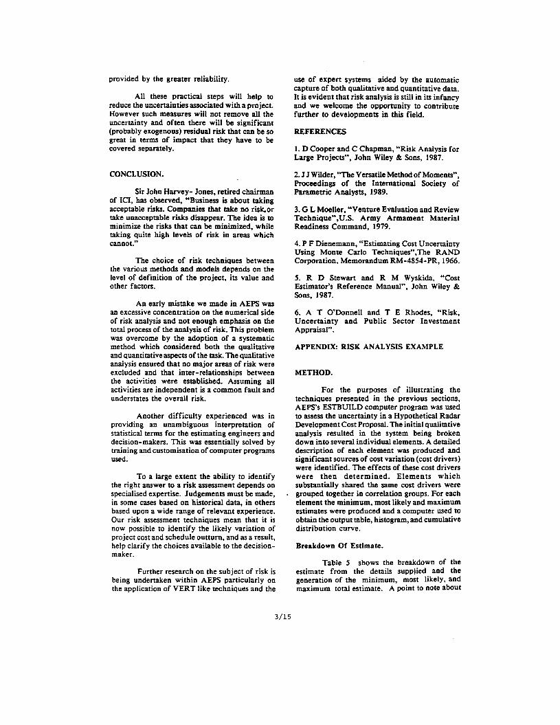
For the purposes of illustrating the techniques presented in the previous sections, AEPS‘s ESTBUILD computer program was used to assess the uncertainty in a Hypothetical Radar Development Cost Proposal. The initial qualitative analysis resulted in the system being broken down into several individual elements. A detailed description of each element was produced and significant sources of cost variation (cost drivers) were identified. The effects of these cost drivers were then determined. Elements which substantially shared the same cost drivers were grouped together in correlation groups. For each element the minimum, most likely and maximum estimates were produced and a computer used to obtain the output table, histogram, and cumulative distribution curve.

Breakdown Of Estimate.

Table 5 shows the breakdown of the estimate from the details supplied and the generation of the minimum, most likely, and maximum total estimate. A point to note about

3/15

Op Code

+

+ + + + + + +

TOT

the overall maximum and minimum values is that they represent the estimator’s opinion of the absolute range of the estimate - there is, however, a very minute chance that these values would occur in practice.

Elements Minimum Most Maximum Description Estimate Likely Estimate

Aerial 8 9 15 Transmitter

Sig. Gen. I5 20 30 Amp 14 15 26

20 22 30 20 2s 50

Receiver Power Supply Processor 4 5 10 Display 3 4 7 Integration . 1 2 6

TOTAL COST fM 85 102 174

Radar Development Costs Frroucncv

94 SO 104 109 114 119 124 129 134 Catm

Figure I I ESTBUILD Frequency Histogram

INTERPRETATION OF RESULTS.

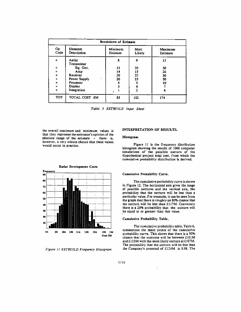
Histogram.

Figure 11 is the frequency distribution histogram showing the results of 1000 computer simulations of the possible outturn of the Hypothetical project total cost, from which the cumulative probability distribution is derived.

Cumulative Probability Curve.

The cumulative probability curve is shown in Figure 12. The horizontal axis gives the range of possible outturns and the vertical axis, the probability that the outturn will be less than a particular value. For example, it can be seen from the graph that there is roughly an 80% chance that the outturn will be less than f 117M. Conversely there is a 20% probability that the outturn will be equal to or greater than this value.

Cumulative Probability Table.

The cumulative probability table, Table 6, summarizes the main points of the cumulative probability curve. This shows that there is a 90% chance that the outcome will be between f lOlM and f 123M with the most likely outturn at f 107M. The probability that the outturn will be less than the Company’s proposal of f124M is 0.98. The

3/16

Radar Development Costs Probabiity

Description Value Probability that fM out-turn is less

than value. Lower 90% 101 0.05 “onfidence limit

94 99 104 109 114 119 124 129 IS4 cntf?d

Lost likely estimat Mean estimate Jpper 90% zonfidence limit Company’s estimate

Figure 12 Cumulative Probability Curve

I 107 0.30 111 0.60 I23 0.95

124 0.98

supplier, in this case, has very little chance that his proposal price will be exceeded.

~ ~~

Table 6 Cumulative Probability Table

COPYRIGHT.

Copyright (C) Controller HMSO London 1991

3/17