Spatial Competition and Pricing in the Agricultural Chemical Industry

R. Lee Hall, Jeffrey H. Dorfman, and Lewell F. Gunter The University of Georgia

Paper for presentation at the 2004 American Agricultural Economics Association Annual Meeting

May 2004

Abstract Three theories of spatial competition are tested on retail price data for the agricultural chemical industry. The empirical tests find only weak evidence of any spatial competition using primary data from sixty-five retailers and twelve different chemicals. Demand and supply-side variables have statistically significant, but economically trivial impacts on retail chemical prices. Competition in the local retail chemical markets appears to have virtually no effect on the retail chemical prices. These results point indirectly to a virtually complete control of retail prices by the chemical manufacturers, likely through the rebate program they offer retailers. The oligopoly structure of the chemical manufacturing industry makes such control possible. The results suggest that consolidation of retailers or distributors will not have anti-competitive effects since price competition is essentially absent from this market already.

© 2004 by R. Lee Hall, Jeffrey H. Dorfman, and Lewell F. Gunter. Please do not cite with permission.

Contact author: Jeffrey Dorfman, Ag. & Applied Economics, Univ. of Georgia, 312 Conner Hall, Athens GA 30602-7509. ph: 706.542.0754. email: jdorfman@agecon.uga.edu.

Agricultural Chemical Industry Introduction

The U.S. Department of Commerce (2001) estimated U. S. farm production expenses for

the fertilizer and chemical industry totaled $18.5 billion dollars in 1999. Insecticides, herbicides,

pesticides, and fungicides are important subcategories of these major expenses, reaching

approximately $8.8 billion in the U.S. in 1997. Without these expenditures, serious damage to

crops would result, causing a drop in both quality and yield. Pesticides have been a growing

source of crop protection since the post-World War II era, and have contributed to the high

productivity of U.S. agriculture (ERS, 2000). Since widespread farmer adoption of chemicals on

crops in the 1940s (MacIntyre, 1987), use has steadily increased, with fluctuations correlated

with crop prices.

A study by Knutson & Associates (1990) describes the possible effects of a ban on

pesticides. The study finds that U.S. farmers would be less competitive in a global market and

major exports, such as corn, wheat, and peanuts, would drop 27%. The study also reveals

farmers in warm, humid climates, i.e. the southern United States, would be harmed more because

such weather promotes higher pest populations. Another study, conducted by GRC Economics

(1989), focuses on a ban of fungicides only. The authors find that U.S. peanut production would

decrease 68% if fungicides were not used. The study also estimates that overall consumer food

prices would increase 13%. Therefore, both farmers and consumers are affected by these inputs.

There are many factors influencing pesticide prices. A partial list includes: commodity

prices, overall health of the agricultural economy, regulations and standards, marketing and

advertising, effectiveness of the product, and safety of the product. These factors have a macro

effect on price, meaning most of these factors are included in price whether the pesticide is

purchased in California or Georgia. The current study focuses on micro level factors affecting

the chemical price, including spatial competition and demand shifting components. Thus, macro

factors will not be included in our econometric model, as we strive to focus on the spatial

component of retail pricing for agricultural chemicals. In this study, we will test the hypothesis

that spatial competition in the agricultural pesticide market has a significant effect on the retail

price of these chemicals. Before testing this hypothesis, we will lay out some of the relevant

theory and previous work, move on to a discussion of our data, and then present the model and

test results.

Theory and Previous Literature

Supply Side Issues

It is estimated that today it costs between $70 and $100 million dollars to research and

develop a new chemical compound for the global market. This creates an obvious incentive to

consolidate and gain scale economies and the incentive is working. In 1996, ten large chemical

manufacturing firms dominated the chemical manufacturing industry worldwide; today, these ten

firms have been reduced to six: Bayer Crop Science, Syngenta, Monsanto, DuPont, Dow

AgroScience, and BASF. The annual sales of these six companies were $22.70 billion for the

year 2000 (Clay, 2001). Clearly, the industry is moving more toward an oligopoly market

structure. From the farmer’s point of view, most experts agree that the concentration of the firms

has been positive with chemical input prices dropping and yields increasing during the period of

consolidation (Clay, 2001).

However, retailers may not have the same point of view as farmers. Leroux, Wortman,

and Mathis (2001) state that “consolidation of the pesticide industry has allowed the companies

2

to more thoroughly control prices both through online outlets and through local outlets.”

Chemical retailers do not deal directly with manufacturers, but are tied to them indirectly

through a rebate system in which manufacturers provide money directly to the retailers at the end

of the year. Most chemical retailers purchase pesticides at a distribution center which buys

directly from the manufacturers. The retailer pays the specified price of the product within

fifteen days of the purchase to the distributor. The retailer in turn charges the farmer the

wholesale price, plus their mark-up, and minus an adjustment to account for the expected rebate

from the manufacturer. The chemical sales representative for each company provides each

individual store with anticipated amounts of rebates.1 Thus, manufacturers play an important

role in the retail pricing of pesticides, able to adjust the retail pricing level of their products

through manipulation of the rebates.

The agricultural chemical market is a high touch industry, requiring large amounts of

customer service and customer interaction. Farmers are accustomed to one-on-one, face-to-face

transactions when purchasing chemical inputs. Farmers are dependant on retailers to provide the

products needed and advice on using the products in the most beneficial way in their area. In

many cases a farmer relies more on trusted individuals’ recommendations than on published

production information (Barry, et al., 1998). Retailers provide customer service representatives

to visit farmers, provide advice, and make sure the chemical application process and rates are

correct. In other cases, a representative from the chemical manufacturer will provide advice

directly to the farmer or supply the retailer with information to pass on the customer. Moss

(2001) argues that these factors make chemical buying decisions fundamentally driven by

personal relationships, significantly diminishing price competition among retailers.

1 It is unclear whether every store receives the same level of rebate or even if rebates are based on a single formula. It was deemed extremely unlikely that firms would provide this type of sensitive financial information for the study; therefore rebate details were not sought.

3

Most chemical retail stores do not deliver, at least not free of charge. Thus, an f.o.b.

pricing scheme is standard and assumed throughout this study.

Demand Side Issues

The United States is the largest purchaser and user of pesticides in the world, with 33%

of worldwide pesticides sales within the U.S. borders (McEwan and Deen, 1997). The USDA’s

Farm Production Expenditures report for the 2001 crop estimates U.S. farm production expenses

at $197 billion dollars with agricultural chemicals making up 4.4% or $8.6 billion. The average

chemical expenditures per farm in 2001 were $3,996. However, the statistics are much higher

for crop farms in the United States, with average expenditures on agricultural chemicals of

$8,170. The Southeast Region, which includes farms in Alabama, Florida, Georgia, and South

Carolina, has much lower total farm expenses than the national average, but chemical

expenditures make up a larger percentage of their expenses at 5%, or $3,818. In Georgia, the

source of this study’s data, pesticides made up 4.1% or $76.34 million in expenses (NASS,

2001).

Farmers’ decisions of what chemicals to buy in what quantity are a function of acreage

grown, types of crops, and economic conditions (McEwan and Deen, 1997). The makeup of the

chemical bundle to be purchased will change from year-to-year and throughout the growing

season based on pest cycles, weather conditions, and commodity prices. These three factors help

determine if pesticide applications are economically justified. For example, it would be

unjustified to apply a pesticide to a crop if the cost of the application would exceed the benefit

obtained. This could be this case in if the crop price was extremely low, pests could not be

controlled, or drought had already caused excessive crop damage. Throughout the growing

season farmers will make numerous purchases of chemicals. The decision of where to purchase

4

inputs is not, and should not be, straightforward. As any savvy consumer understands, it is

important to compare prices and shop around.

Studies of the demand for pest control have generally concluded farmers’ pest control

purchasing decisions are relatively inelastic with respect to product price (Fernandez-Cornjeo

and Jans, 1995; McIntosh and Williams, 1992). Norgaard (1976) argued farmers also appear to

be “irrational” in their pesticide use, using more than the profit-maximizing amount. This

“irrational” behavior is most likely attributed to risk aversion on the part of the farmer. Fox and

Weersink (1995) define pesticides as a class of inputs called damage control inputs, recognizing

their role in risk reduction as well as profit generation. Specific chemical purchases are also

highly substitutable across brands. Thus, small price changes can result in significant changes in

the mix of products used as farmers attempt to maximize profits. For example, a farmer may

choose between Orthene 75S and Dipel to control an insect problem depending on price of each

product. Both products control many of the same pests and the only difference may be in the

price. This high cross-price elasticity of demand for specific chemicals should increase

competition among retailers (and/or manufacturers and distributors) without contradicting the

inelastic overall demand for chemicals since aggregate purchases are unaffected (ERS, 2000).

As in any industry, retailers have to meet the needs of the customers. One way the

agricultural chemical retailers do this is through establishing a line of credit for farmers. This

helps farmers with liquidity issues and convenience, saving time and allowing employees to

purchase (pickup) chemicals without trusting those employees with a company checkbook.

Once the chemical purchase has been made the farmer normally faces three payment options:

pay at the time of purchase, pay monthly, or pay at the end of the season. The third option will

generally involve paying accrued interest charges in addition to the chemical purchase price.

5

However, in the world of chemical sales, like most industries, not everyone is equal. Farmers

who purchase large quantities of product normally receive a bulk discount (and may receive

more favorable payment terms). Such rewards for large customers suggest that the presence of

large-scale commercial farmers may influence the degree of price competition observed among

retailers.

Spatial Competition

The most natural criterion for the separation of consumers and individual consumer

markets is a spatial one. Households, farms, and businesses exist, purchase and consume in a

spatial environment. Products are manufactured at one location and then distributed to various

and numerous markets. When one includes factors such as transportation costs and general

frictions of distance such as loss of information and inconvenience, markets are more clearly

understood in a spatial environment. Capozza and Van Order (1978) state two essential

distinguishing features of spatial competition: transportation costs and downward sloping

average costs curves over some range of quantity sold. In the modern world, transportation costs

include shipping costs for remote purchases and must vary across possible purchase sites to make

location matter. Average costs curves are assumed to be negatively sloped within some quantity

range (due to economies of scale or fixed costs) since otherwise there would no advantage to

concentrating production.

With spatially distributed, competing firms, each firm’s price behavior is also partially

dependent on its belief concerning the price responses of its competitors. These beliefs are

referred to as conjectural variations since it is the firm’s “conjecture” that counts. The three

main conjectural variations considered in the analysis of spatial economic theory (Greenhut,

Norman, and Hung, 1987) are Löschian competition, Hotelling-Smithies competition, and

6

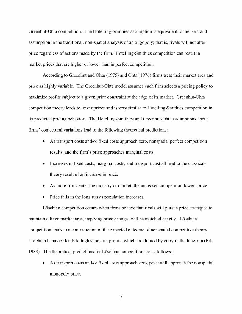
Greenhut-Ohta competition. The Hotelling-Smithies assumption is equivalent to the Bertrand

assumption in the traditional, non-spatial analysis of an oligopoly; that is, rivals will not alter

price regardless of actions made by the firm. Hotelling-Smithies competition can result in

market prices that are higher or lower than in perfect competition.

According to Greenhut and Ohta (1975) and Ohta (1976) firms treat their market area and

price as highly variable. The Greenhut-Ohta model assumes each firm selects a pricing policy to

maximize profits subject to a given price constraint at the edge of its market. Greenhut-Ohta

competition theory leads to lower prices and is very similar to Hotelling-Smithies competition in

its predicted pricing behavior. The Hotelling-Smithies and Greenhut-Ohta assumptions about

firms’ conjectural variations lead to the following theoretical predictions:

• As transport costs and/or fixed costs approach zero, nonspatial perfect competition

results, and the firm’s price approaches marginal costs.

• Increases in fixed costs, marginal costs, and transport cost all lead to the classical-

theory result of an increase in price.

• As more firms enter the industry or market, the increased competition lowers price.

• Price falls in the long run as population increases.

Löschian competition occurs when firms believe that rivals will pursue price strategies to

maintain a fixed market area, implying price changes will be matched exactly. Löschian

competition leads to a contradiction of the expected outcome of nonspatial competitive theory.

Löschian behavior leads to high short-run profits, which are diluted by entry in the long-run (Fik,

1988). The theoretical predictions for Löschian competition are as follows:

• As transport costs and/or fixed costs approach zero, price will approach the nonspatial

monopoly price.

7

• As fixed costs and transport costs rise, price falls, whereas an increase in marginal

costs leads to ambiguous results.

• As firms enter and thus competition increases, prices increases.

• Price increases as population density, or consumers, increases.

Very few studies have been done on spatial competition in the agribusiness sector. Fik

(1988) studied spatial competition in food markets or supermarkets. He theorized that price

competition in the retail food markets is highly dependent on the location and/or the distance to

rival firms. His results concluded a solid link between price, space and the intensity of price

reaction as a decreasing function of distance. Durham, Sexton, and Ho Song (1996) examined

the role of spatial pricing in the allocation of tomatoes from farms to processing facilities across

the state of California. The aim of the study was to determine if the tomato farmers were

shipping the product to the most profitable processing facilities. The results indicated farmers

were hauling the tomatoes an extra 10 miles per trip to the processing plant. This misallocation

was estimated to cost an extra $7.41 million dollars in transportation costs; however, this

represented only a 1.9% loss from potential industry-wide profit.

Empirical Testing

Model Definition

To test these theories of spatial competition in the retail-level U.S. agricultural chemical

industry, a retailer mail survey was conducted in Georgia and the data were used to estimate an

econometric model of chemical pricing for twelve different, commonly used agricultural

chemicals.

8

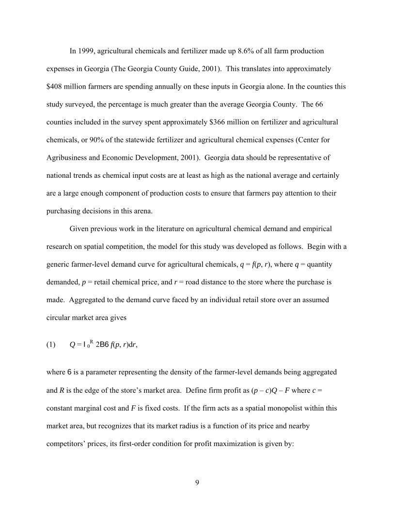
In 1999, agricultural chemicals and fertilizer made up 8.6% of all farm production

expenses in Georgia (The Georgia County Guide, 2001). This translates into approximately

$408 million farmers are spending annually on these inputs in Georgia alone. In the counties this

study surveyed, the percentage is much greater than the average Georgia County. The 66

counties included in the survey spent approximately $366 million on fertilizer and agricultural

chemicals, or 90% of the statewide fertilizer and agricultural chemical expenses (Center for

Agribusiness and Economic Development, 2001). Georgia data should be representative of

national trends as chemical input costs are at least as high as the national average and certainly

are a large enough component of production costs to ensure that farmers pay attention to their

purchasing decisions in this arena.

Given previous work in the literature on agricultural chemical demand and empirical

research on spatial competition, the model for this study was developed as follows. Begin with a

generic farmer-level demand curve for agricultural chemicals, q = f(p, r), where q = quantity

demanded, p = retail chemical price, and r = road distance to the store where the purchase is

made. Aggregated to the demand curve faced by an individual retail store over an assumed

circular market area gives

(1) Q = I0

R 2B6 f(p, r)dr,

where 6 is a parameter representing the density of the farmer-level demands being aggregated

and R is the edge of the store’s market area. Define firm profit as (p – c)Q – F where c =

constant marginal cost and F is fixed costs. If the firm acts as a spatial monopolist within this

market area, but recognizes that its market radius is a function of its price and nearby

competitors’ prices, its first-order condition for profit maximization is given by:

9

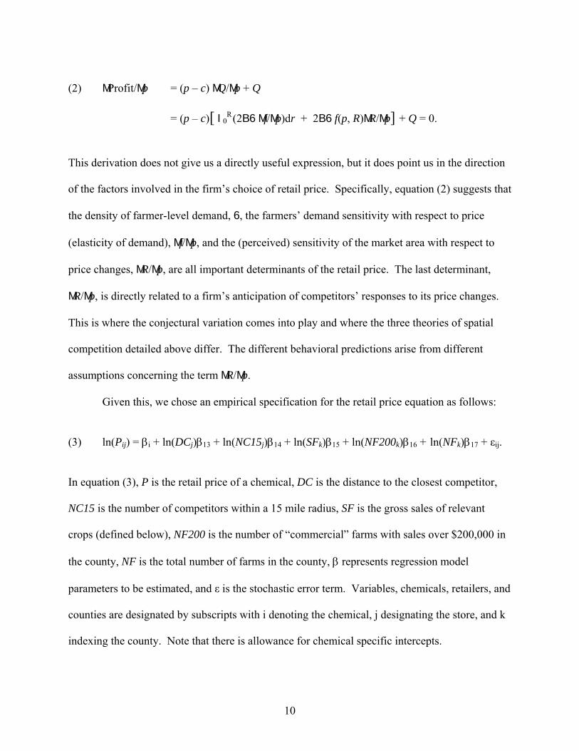
(2) MProfit/Mp = (p – c) MQ/Mp + Q

= (p – c)[ I0R (2B6 Mf/Mp)dr + 2B6 f(p, R)MR/Mp] + Q = 0.

This derivation does not give us a directly useful expression, but it does point us in the direction

of the factors involved in the firm’s choice of retail price. Specifically, equation (2) suggests that

the density of farmer-level demand, 6, the farmers’ demand sensitivity with respect to price

(elasticity of demand), Mf/Mp, and the (perceived) sensitivity of the market area with respect to

price changes, MR/Mp, are all important determinants of the retail price. The last determinant,

MR/Mp, is directly related to a firm’s anticipation of competitors’ responses to its price changes.

This is where the conjectural variation comes into play and where the three theories of spatial

competition detailed above differ. The different behavioral predictions arise from different

assumptions concerning the term MR/Mp.

Given this, we chose an empirical specification for the retail price equation as follows:

(3) ln(Pij) = βi + ln(DCj)β13 + ln(NC15j)β14 + ln(SFk)β15 + ln(NF200k)β16 + ln(NFk)β17 + εij.

In equation (3), P is the retail price of a chemical, DC is the distance to the closest competitor,

NC15 is the number of competitors within a 15 mile radius, SF is the gross sales of relevant

crops (defined below), NF200 is the number of “commercial” farms with sales over $200,000 in

the county, NF is the total number of farms in the county, β represents regression model

parameters to be estimated, and ε is the stochastic error term. Variables, chemicals, retailers, and

counties are designated by subscripts with i denoting the chemical, j designating the store, and k

indexing the county. Note that there is allowance for chemical specific intercepts.

10

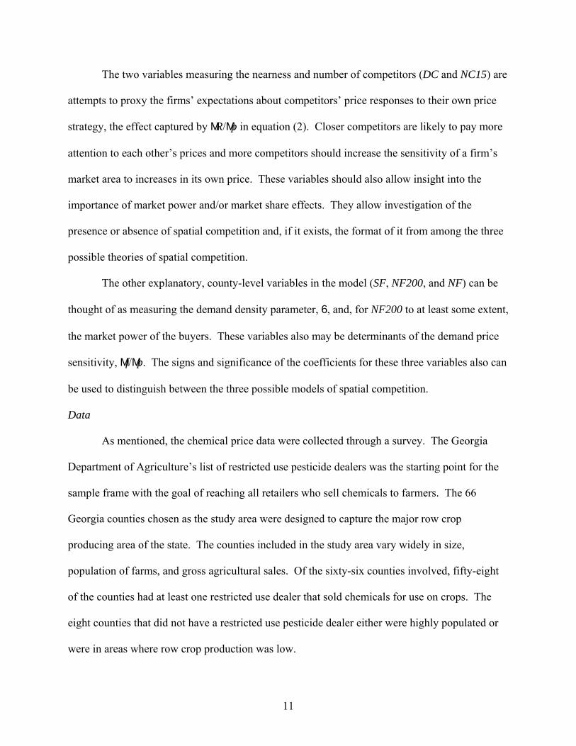
The two variables measuring the nearness and number of competitors (DC and NC15) are

attempts to proxy the firms’ expectations about competitors’ price responses to their own price

strategy, the effect captured by MR/Mp in equation (2). Closer competitors are likely to pay more

attention to each other’s prices and more competitors should increase the sensitivity of a firm’s

market area to increases in its own price. These variables should also allow insight into the

importance of market power and/or market share effects. They allow investigation of the

presence or absence of spatial competition and, if it exists, the format of it from among the three

possible theories of spatial competition.

The other explanatory, county-level variables in the model (SF, NF200, and NF) can be

thought of as measuring the demand density parameter, 6, and, for NF200 to at least some extent,

the market power of the buyers. These variables also may be determinants of the demand price

sensitivity, Mf/Mp. The signs and significance of the coefficients for these three variables also can

be used to distinguish between the three possible models of spatial competition.

Data

As mentioned, the chemical price data were collected through a survey. The Georgia

Department of Agriculture’s list of restricted use pesticide dealers was the starting point for the

sample frame with the goal of reaching all retailers who sell chemicals to farmers. The 66

Georgia counties chosen as the study area were designed to capture the major row crop

producing area of the state. The counties included in the study area vary widely in size,

population of farms, and gross agricultural sales. Of the sixty-six counties involved, fifty-eight

of the counties had at least one restricted use dealer that sold chemicals for use on crops. The

eight counties that did not have a restricted use pesticide dealer either were highly populated or

were in areas where row crop production was low.

11

The retailers were each contacted via telephone and asked two questions. The first

question was: does your firm sell pesticides for use on farms? If the firm answered ‘yes’ then the

firm was asked for their fax number. If the answer was ‘no’ then they were eliminated from the

list of potential survey participants. Since the firms did not sell chemicals that were used by

farms, it was assumed the firm either sold pesticides for home pest control or other pesticides not

related to farming. Thus, the survey was sent to the entire population of retailers in the study

area.

The survey faxed to each retailer asked the firm to provide the retail price paid by the

average farmer for twelve highly used agricultural chemicals. Of the 204 surveys faxed out, 65

were returned, for a response rate of 32%. Not all the responders provided prices for all the

chemicals; however, overall there were 552 prices responses from the 65 responding retailers.

These responses comprise the price data for this study. The names of the twelve chemicals and

summary details of the responses can be found in table 1.

The remaining variables were constructed from secondary data. The two spatial

competition measures (DC and NC15) were constructed using Microsoft Map Quest and the firm

addresses in the original RUP list from the Georgia Department of Agriculture. The fifteen mile

radius for the NC15 variable was chosen as an approximation of how far a farmer was willing to

travel to purchase these chemicals; any stores farther away were deemed to far to expect a farmer

to travel, particularly given that this is direct distance, not road mileage. While this is an

arbitrary definition of potential market area for a firm, it seems a reasonable one given the

demands on farm labor time and the transportation cost associated with these (bulky) chemicals.

The average distance between competitors is 5.83 miles, the longest distance between

competitors is 18.7, and the shortest distance is 0.3 miles.

12

The number of total and commercial farms in each county (NF and NF200) was obtained

from USDA’s 1997 Census of Agriculture.2 The value of (relevant) farm production in each

county (SF) was computed by summing county-level value data for row and forage crops, fruits

and nuts, vegetables, ornamental horticulture, and forestry production (Center for Agribusiness

and Economic Development, 2002). Categories included are those crops most reliant on the

surveyed chemicals.

Estimation Approach and Diagnostics

The model was estimated using generalized least squares (GLS) to account for chemical-

specific heteroscedasticity. That is, the model error variance was allowed to vary by chemical,

but was held constant for all observations on each chemical. Diagnostic testing for firm-specific

and regional heteroscedasticity found no evidence of such effects. The condition number for the

model data matrix is 387, so multicollinearity is not a particular problem with this data set.

Spatial autocorrelation is a potential problem for the regression model given that the data

is spatial in nature and space is an integral part of the hypotheses we wish to test. Therefore,

Moran’s I test was performed to test for the presence of spatial autocorrelation (Moran, 1950).

Moran’s I test uses the residuals from an initial OLS regression on the model being tested

estimation to test for spatial autocorrelation, and is defined as:

(2) I = [ ( 3i 3j wijeiej )/ ( 3i 3j wij ) ]/ [(n-k)s2/n] ,

where wij is a binary variable equal to one if observations i and j are “neighbors,” ei is the ith

residual from the OLS regression, n is the number of observations in the data set, k is the number

of estimated regressors, s2 is the standard OLS estimator of the error variance, and the

summations are all from i (or j) =1, 2., …, n. When spatial autocorrelation is present, Moran’s I

test statistic is greater than one. 2 Table 6: Farms, Land in Farms, and Value of Land and Buildings, and Land Use: 1997 and 1992.

13

Two chemicals were tested for spatial autocorrelation: Temik® and RoundUp®

UltraMax (2.5 gallon); these are the most popular chemicals and the data set contained the most

observations for these two, meaning the test would have the most power in these cases. The

results of the Moran’s I test, displayed in table 2, reveal no statistical evidence in favor of spatial

autocorrelation; both the test statistics are negative and the z-scores of the two test statistics are

considerably below the one-tail critical value of 1.645 for a 0.05 significance level. Therefore,

the GLS model is assumed free of spatial autocorrelation.

Results: Statistical versus Economic Significance

The results of the regression model estimation are shown in table 3. The key result is that

the coefficients on the two variables most closely linked to spatial competition, DC and NC15,

are both statistically and economically insignificant. Thus, these coefficients don’t offer

empirical evidence in favor of spatial competition to the retail agricultural chemical market.

The coefficients on the demand-side variables are all statistically significant, but are

pretty minor in terms of economic impact (recall that all the coefficients are elasticities due to the

double-log form). For example, the price elasticity with respect to the number of farms (NF) is

0.0822. With a t-value of over 5, this coefficient is very precisely estimated, but the economic

impact is trivial. The number of farms would have to decrease by 12% to cause chemical prices

to decrease by 1%. The price elasticity with respect to the number of commercial farms (NF200)

is approximately the same magnitude, but of opposite sign with a point estimate of -0.0798.

Since a possible scenario is for the total number of farms to shrink while commercial farms

increase (through consolidation), one could anticipate some decrease in agricultural chemical

prices over time. This makes sense if retailers need to price more competitively to attract the

14

business of larger farms which are more likely to shop carefully given the larger expense of

buying chemicals in higher quantities.

The estimated price elasticity with respect to gross farm sales (SF) is also statistically

significant, but economically insignificant. An increase in sales, assumedly linked to an increase

in the total quantity of chemicals purchased, leads to a slightly lower price. This is consistent

with Hotelling-Smithies and Greenhut-Ohta competition, but not with the Löschian theory.

However, this evidence in favor of two of the theories of spatial competition relative to the third

cannot be considered particularly strong given the magnitude of the elasticity (point estimate of -

0.0289) and the insignificance of the other, more obvious, spatial competition variables.

Statistical significance without economic significance seems a low hurdle for an economic

theory to clear.

Conclusions

The main finding of this study is the lack of spatial competition among agricultural

chemical retailers, even though the average distance between retailers was less than six miles.

Only weak evidence in favor of spatial competition can be found, with that evidence leaning

toward Hotelling-Smithies or Greenhut-Ohta style competition. The level of competition in the

retail chemical markets appears to be unrelated to the level of retail chemical prices.

This surprising finding suggests that the oligopoly structure of the chemical

manufacturers and distributors, combined with the manufacturers’ rebate programs, has given

them tight control over retail prices. One policy implication of this finding is that there is little

point in worrying about consolidation among chemical distributors and retailers as retail prices

seem unlikely to rise if “competition” is reduced.

15

We also find that prices are controlled firmly enough by manufacturers and distributors

that demand-side shifters do not have much impact on retail prices either. While we measured

statistically significant effects of the demand-side variables included in the regression model, the

economic magnitude of these effects is trivial.

16

References

Barry, P.J., Sotomayor, N., and L.A. Moss. “Professional Farm Manager’s View on Leasing

Contracts and Land Control: An Illinois Perspective.” Journal of the American Society of

Farm Managers and Rural Appraisers. Vol. 62 (1998-1999): 15-19.

Capozza, D.R., and Van Order, R., “A Generalized Model of Spatial Competition.” The

American Economic Review. Vol. 68 No. 5 (December 1978): 896-908.

Center for Agribusiness & Economic Development, College of Agriculture and Environmental

Sciences, University of Georgia. The Georgia County Guide. 2001

Center for Agribusiness & Economic Development, College of Agriculture and Environmental

Sciences, University of Georgia. The Georgia Farmgate Value Report 2001. 2002

Clay, Heather. “Agro Chemical Giants- Keeping track of the names.” Hivelights. Vol. 14 No. 4

(November 2001).

Durham, C.A., Sexton, R.J., and Ho Song, J. “Spatial Competition, Uniform Pricing, and

Transportation Efficiency in the California Processing Tomato Industry.” American

Journal of Agricultural Economics. Vol. 78 Issue 1 (February 1996): 115-125.

Fernandez-Cornejo, J., and Jans, S. “Quality-Adjusted Price and Quantity Indices for

Pesticides.” American Journal of Agricultural Economics. Vol. 77 Issue 3 (August

1995): 645-659.

Fik, T.J., “Spatial Competition and Price Reporting in Retail Food Markets,” Economic

Geography, Vol. 64 Issue 1 (January 1988): 29-44.

Fox, G. and Weersink, A., “Damage Control and Increasing Returns.” American Journal of

Agricultural Economics. Vol. 77 Issue 1 (February 1995): 33-39.

17

GRC Economics. “The Value of Fungicides to the Availability of a Healthy and Affordable

Food Supply.” Washington, D.C. (1989).

Greenhut M.L., Norman, G., and Hung, C., The Economics of Imperfect Competition: A Spatial

Approach. New York: Cambridge University Press, 1987.

Greenhut, M.L., and Ohta, H., “Monopoly Output Under Alternative Spatial Pricing

Techniques.” American Economic Review Vol. 62 Issue 4 (July1975): 705-713.

Knutson, R.D., Taylor, J.B., & E.G. Smith. Economic Impacts of Reduced Chemical Use.

Knutson & Associates, College Station, Texas. 1990.

Leroux, N., Wortman, M.S., and Mathias, E., “Dominant Factors Impacting the Development of

Business-to-Business (B2B) E-Commerce in Agriculture.” Paper presented at the 2001

IAMA Symposium in Sydney, Australia, June 27-28, 2001.

MacIntyre, A.A., “Why Pesticides Received Extensive Use in America: A Political Economy of

Agricultural Pest Management to 1970.” Natural Resource Journal Vol. 27 Summer

Issue (1987).

McEwan, B., and Deen, K., “A Review of Agriculture Pesticides Pricing and Availability in

Canada. University of Guelph. 1997.

McIntosh, C.S., and Williams, A.A., “Multiproduct Product Choices and Pesticide Regulation in

Georgia.” Southern Journal of Agricultural Economics. Vol. 24 Issue 1 (July, 1992):

135-144.

Moran, P.A.P., “Partial and Multiple Rank Correlation.” Biometrika Vol. 37 Issue1/2

(June,1950): 26-32.

Moss, L.A. “Who Wins and Loses and How Will E-Markets Affect Rural America?” Paper

presented at the USDA Outlook Forum, Washington, DC, February, 2001.

18

Norgaard, R.B., “The Economics of Improving Pesticide Use.” Annual Review of Entomology.

Vol. 21 (1976): 45-60.

Ohta, H., “On the Efficiency of Production Under Conditions of Imperfect Competition.”

Southern Economic Journal Vol. 43 Issue 2 (October 1976): 1124-35.

U.S. Department of Agriculture, Economic Research Service, Agricultural Resources and

Environmental Indicators. (October, 2000): Chapter 4.3.

U.S. Department of Agriculture. National Agriculture Statistics Service. 1997 Census of

Agriculture—County Data. Table 6 – Farms, Land in Farms, Value of Land and

Buildings, and land Use: 1997 and 1992.

U.S. Department of Agriculture. National Agriculture Statistics Service. Farm Computer Usage

and Ownership Report. July 2001.

U.S. Department of Agriculture. National Agriculture Statistics Service. Farm Production

Expenditures 2001 Summary. July 2002.

U.S. Department of Commerce. “Farm Income and Farm Production Expenses” May 2001,

Table CA45, Regional Economic Information System, Bureau of Economic Analysis,

U.S. Department of Commerce, Washington, D.C.

19

Table 1: Chemical Price Response Summary

Chemical Count Counties Included

Max ($) Min ($)

Mean ($) STD($)

Temik® 64 36 3.49 2.95 3.09 0.11

Round-Up®(2.5) 57 32 55 33.35 45.64 4.08

Round-Up®(bulk) 48 29 46.90 37.40 40.11 2.12

Glyfos® X-TRA (2.5) 44 30 42 19 27.95 5.98

Glyfos® X-TRA(bulk) 32 24 35.25 18.5 23.39 4.31

Prowl® 3.3 EC 63 36 34 13 18.84 2.72

Orthene®75S 40 29 17 7.5 10.39 1.51

Orhtene®90S 53 34 12 7.5 9.29 0.76

Bravo® 720 42 29 55 35 39.50 3.72

Chlorothalonil 29 23 32 55 37.75 4.35

Trilin® 27 19 21 10.65 15.96 2.23

Trifluralin HF 52 32 22.5 8.95 15.29 2.06

20

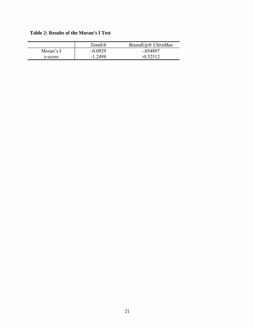
Table 2: Results of the Moran’s I Test

Temik® RoundUp® UltraMax Moran’s I -0.0929 -.054897

z-score -1.2498 -0.52512

21

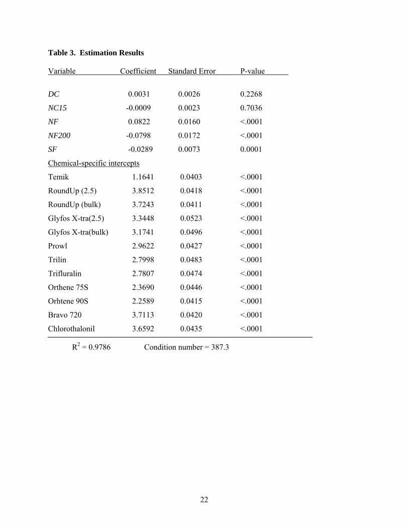
Table 3. Estimation Results

Variable Coefficient Standard Error P-value

DC 0.0031 0.0026 0.2268

NC15 -0.0009 0.0023 0.7036

NF 0.0822 0.0160 <.0001

NF200 -0.0798 0.0172 <.0001

SF -0.0289 0.0073 0.0001

Chemical-specific intercepts

Temik 1.1641 0.0403 <.0001

RoundUp (2.5) 3.8512 0.0418 <.0001

RoundUp (bulk) 3.7243 0.0411 <.0001

Glyfos X-tra(2.5) 3.3448 0.0523 <.0001

Glyfos X-tra(bulk) 3.1741 0.0496 <.0001

Prowl 2.9622 0.0427 <.0001

Trilin 2.7998 0.0483 <.0001

Trifluralin 2.7807 0.0474 <.0001

Orthene 75S 2.3690 0.0446 <.0001

Orhtene 90S 2.2589 0.0415 <.0001

Bravo 720 3.7113 0.0420 <.0001

Chlorothalonil 3.6592 0.0435 <.0001 R2 = 0.9786 Condition number = 387.3

22

Appendix: List of Surveyed Chemicals Temik® is a restricted use pesticide for the control of insects, mites and nematodes. Aventis CS

is the manufacturer of this product, which has a generic, or common, name of Aldicarb.

Temik® is used on peanuts, cotton, soybeans, and tobacco3 at planting to control a

variety of pests in the surveyed region.

Round-Up® UltraMax is a popular herbicide that is used on a variety of crops in the survey area.

The generic name is Glyphosphate, and has many competitors. The introduction of

genetically modified crops, such as Round-Up ready cotton has greatly increased the

demand of this product. Round-Up® Ultramax is a product of the Monsanto, and in sold

in three different ways: 2.5-gallon containers, 30 gallon drums, and in bulk. The survey

included price questions for the 2.5-gallon containers and in bulk.

Glyfos® X-TRA is a popular generic herbicide, Glyphosphate, that is direct competition with

Round-Up® Ultramax. It is used on the same crops and sold in the same forms: 2.5-

gallon containers, 30-gallon drums, and bulk. Price was collected on 2.5-gallon

containers and in bulk.

Prowl® 3.3 EC is a herbicide used on cotton, fruit & nut crops, peanuts, soybeans, and a variety

of vegetable crops. The generic name is pendimethalin, and it is manufactured by the

BASF Company. Prowl® 3.3 EC is sold in 2.5-gallon containers.

Trilin® is a selective herbicide for the pre-emergence of annual grasses and broadleaf weeds.

Trilin® is used on a variety of crops including vegetables, soybeans, cotton, and peanuts.

Trilin® is a product of the Griffin Corporation and is sold in 2.5-gallon containers.

3 Temik® is not labeled for tobacco use in Georgia. However, it is widely used on the crop according to many retailers.

23

Trifluralin HF is a product of the UAP company and is a basically the same product as Trilin®.

Again, the chemical is used on the same crops as Trilin® and is sold in 2.5-gallon

containers.

Orthene® 75 S is a water-soluble insecticide powder manufactured by the Valent Corporation.

Orhtene 75 S is composed of 75% of the active ingredient, Acephate. Orhtene 75 S is

used on many crops in the survey region including vegetables, cotton, tobacco, and

peanuts.

Orthene® 90 S is a stronger version of Orthene® 75 S, and is made up of 90% Acephate. Both

Orthene® 75 S and 90 S are sold by the pound in a variety of packing. The surveyed

packing was a 10-lb water-soluble bag.

Bravo® 720 is an agricultural fungicide used mainly on vegetable and peanut crops in the

surveyed region. The generic name is Chlorothalonil. Bravo® 720 is a product of ISK

Biosciences Corporation and is sold in 2.5-gallon containers.

Chlorothalonil is a generic name for Bravo 720 and is manufactured by a variety of chemical

companies. It is also sold in 2.5-gallon containers and is used on the same crops as

Bravo® 720.

24