r-max: a general polynomial time algorithm for near-optimal reinforcement learning
DESCRIPTION
R. Brafman and M. Tennenholtz Presented by Daniel Rasmussen. R-Max: A General Polynomial Time Algorithm for Near-Optimal Reinforcement Learning. Motivation. Exploration versus Exploitation - PowerPoint PPT PresentationTRANSCRIPT

R. Brafman and M. Tennenholtz
Presented by Daniel Rasmussen
Exploration versus Exploitation Should we follow our best known path for a
guaranteed reward, or take an unknown path for a chance at a greater reward?
Explicit policies do not work well in multiagent settings
R-Max uses an implicit exploration/exploitation policy How does it do this? Why should we believe it works?

BackgroundR-Max algorithmProof of near-optimalityVariations on the algorithmConclusions

A set of (normal form) games
Each game has a set of possible actions and rewards associated with those actions as usual
We add a probabilistic transfer function that maps the current game and the players’ actions onto the next game

(2,2)
(3, 1)
(2, 3)
(1, 1)
(4,2)
(1, 1)
(2, 2)
(1, 0)
(0,2)
(5, 1)
(2, 4)
(3, 1)
(4,3)
(3, 3)
(2, 3)
(1, 1)
(2,0)
(3, 0)
(2, 1)
(1, 1)
(5,2)
(0, 1)
(4, 3)
(5, 1)
0.7
0.3
0.2
0.4
0.4

History: the set of all past states, the actions taken in those states, and the rewards received (plus the current state) (S x A2 x R)t x S
Policy: a mapping from the set of histories to the set of possible actions in the current state P: (S x A2 x R)t x S A, for all t >= 0
Value of a policy: expected average reward if we follow the policy for T steps Denoted U(s, pa, po, T) U(pa) = minpominslimT..∞ U(s, pa, po, T)

ε-return mixing time: how many steps do we need to take before the expected average reward is within ε of the stable average Min T such that U(s, pa, po, T) > U(pa) – ε for all s
and po
Optimal policy: the policy with the highest U(pa) We will always parameterize this in ε and T (i.e.
the policy with the highest U(pa) whose ε-return mixing time is T)

The agent always knows what state it is in
After each stage the agent knows what actions were taken and what rewards were received
We know the maximum possible reward, Rmax
We know the ε-return mixing time of any policy

When faced with the choice between a known and unknown reward, always try the unknown reward

Maintain an internal model of the stochastic game
Calculate an optimal policy according to model and carry it out
Update model based on observations
Calculate a new optimal policy and repeat
Input N: number of games k: number of actions in each game ε: the error bound δ: the probability of failure Rmax: the maximum reward value T: the ε-return mixing time of an optimal
policy
Initializing the internal model Create states {G1...Gn} to represent the
stages in the stochastic game Create a fictitious game G0 Initialize all rewards to (Rmax, 0) Set all transfer functions to point to G0 Associate a boolean known/unknown
variable with each entry in each game, initialized to unknown
Associate a list of states reached with each entry, which is initially empty

(2,2)
(3, 1)
(2, 3)
(1, 1)
(4,2)
(1, 1)
(2, 2)
(1, 0)
(0,2)
(5, 1)
(2, 4)
(3, 1)
(4,3)
(3, 3)
(2, 3)
(1, 1)
(2,0)
(3, 0)
(2, 1)
(1, 1)
(5,2)
(0, 1)
(4, 3)
(5, 1)
0.7
0.3
0.2
0.4
0.4
G1
G2
G3
G4
G5
G6

Rmax,0
Rmax,0
Rmax,0
Rmax,0
Rmax,0
Rmax,0
Rmax,0
Rmax,0
Rmax,0
Rmax,0
Rmax,0
Rmax,0
Rmax,0
Rmax,0
Rmax,0
Rmax,0
Rmax,0
Rmax,0
Rmax,0
Rmax,0
Rmax,0
Rmax,0
Rmax,0
Rmax,0
unknown{}
unknown{}
unknown{}
unknown{}
G1
G2
G3
G4
G5
G6
G0

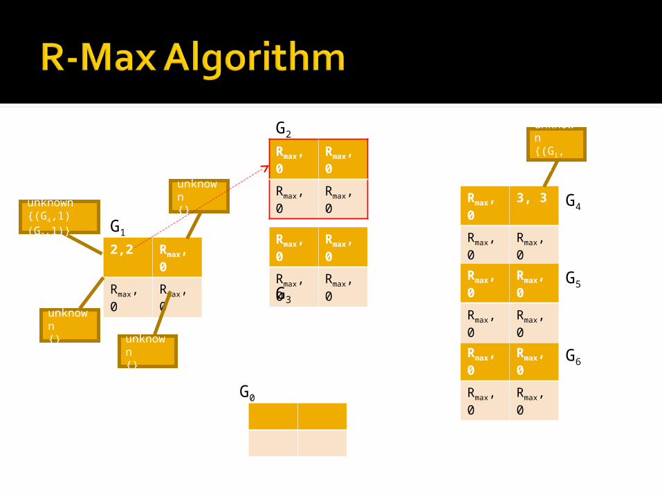
Repeat Compute an optimal policy for T steps based
on the current internal model Execute that policy for T steps After each step:▪ If an entry was visited for the first time, update the
rewards based on observations▪ Update the list of states reached from that entry▪ If the list of states reached now contains c+1
elements▪ mark that entry as known▪ update the transition function▪ compute a new policy

Rmax,0
Rmax,0
Rmax,0
Rmax,0
Rmax,0
Rmax,0
Rmax,0
Rmax,0
Rmax,0
Rmax,0
Rmax,0
Rmax,0
Rmax,0
Rmax,0
Rmax,0
Rmax,0
Rmax,0
Rmax,0
Rmax,0
Rmax,0
Rmax,0
Rmax,0
Rmax,0
Rmax,0
unknown{}
unknown{}
unknown{}
unknown{}
G1
G2
G3
G4
G5
G6
G0

2,2 Rmax,0
Rmax,0
Rmax,0
Rmax,0
Rmax,0
Rmax,0
Rmax,0
Rmax,0
Rmax,0
Rmax,0
Rmax,0
Rmax,0
Rmax,0
Rmax,0
Rmax,0
Rmax,0
Rmax,0
Rmax,0
Rmax,0
Rmax,0
Rmax,0
Rmax,0
Rmax,0
unknown{(G4,1)}
unknown{}
unknown{}
unknown{}
G1
G2
G3
G4
G5
G6
G0

2,2 Rmax,0
Rmax,0
Rmax,0
Rmax,0
Rmax,0
Rmax,0
Rmax,0
Rmax,0
Rmax,0
Rmax,0
Rmax,0
Rmax,0
3, 3
Rmax,0
Rmax,0
Rmax,0
Rmax,0
Rmax,0
Rmax,0
Rmax,0
Rmax,0
Rmax,0
Rmax,0
unknown{(G4,1)}
unknown{}
unknown{}
unknown{}
G1
G2
G3
G4
G5
G6
G0
unknown{(G1,1)}
2,2 Rmax,0
Rmax,0
Rmax,0
Rmax,0
Rmax,0
Rmax,0
Rmax,0
Rmax,0
Rmax,0
Rmax,0
Rmax,0
Rmax,0
3, 3
Rmax,0
Rmax,0
Rmax,0
Rmax,0
Rmax,0
Rmax,0
Rmax,0
Rmax,0
Rmax,0
Rmax,0
unknown{(G4,1)(G2,1)}
unknown{}
unknown{}
unknown{}
G1
G2
G3
G4
G5
G6
G0
unknown{(G1, 1)}

2,2 Rmax,0
Rmax,0
Rmax,0
Rmax,0
Rmax,0
Rmax,0
Rmax,0
Rmax,0
Rmax,0
Rmax,0
Rmax,0
Rmax,0
3, 3
Rmax,0
Rmax,0
Rmax,0
Rmax,0
Rmax,0
Rmax,0
Rmax,0
Rmax,0
Rmax,0
Rmax,0
unknown{}
unknown{}
unknown{}
G1
G2
G3
G4
G5
G6
G0
unknown{(G1, 1)}
0.5
0.5known{(G4,1)(G2,1)}

Goal: prove that if the agent follows the R-Max algorithm for T steps the average reward will be within ε of the optimum
Outline of proof: After T steps the agent will have either obtained
near-optimum average reward or it will have learned something new
There are a polynomial number of parameters to learn, therefore the agent can completely learn its model in polynomial time
The adversary can block learning, but if it does so then the agent will obtain near-optimum reward
Either way the agent wins!

Lemma 1: If the agent’s model is a sufficiently close approximation of the true game, then an optimal policy in the model will be near-optimal in the game We guarantee that the model is
sufficiently close by waiting until we have c + 1 samples before marking an entry known

Lemma 2: the difference between the expected reward based on the model and the actual reward will be less than the exploration probability times Rmax |Vmodel – Vactual| < eRmax
large |Vmodel – Vactual| large exploration probability
Combining Lemma 1 and 2 In unknown states the agent has an
unrealistically high expectation of reward (Rmax), so Lemma 2 tells us that the probability of exploration is high
In known states Lemma 1 tells us that we will obtain near-optimal reward
We will always be in either a known or unknown state, therefore we will always explore with high probability or obtain near-optimal reward
If we explore for long enough then (almost) all states will be known, and we are guaranteed near-optimal reward

Remove assumption that we know the ε-return mixing time of an optimal policy, T
Remove assumption that we know Rmax
Simplified version for repeated games

R-Max is a model-based reinforcement learning algorithm that is guaranteed to converge on the near-optimal average reward in polynomial time Works on zero-sum stochastic games, MDPs,
and repeated games
The authors provide a formal justification for optimism under uncertainty heuristic Guarantee that the agent either obtains near-
optimal reward or learns efficiently

For complicated games N, k, and T are all likely to be high, so polynomial time will still not be computationally feasible
We do not consider how the agent’s behaviour might impact the adversary’s