RULES OF THUMB AND DYNAMICPROGRAMMING�By Martin Lettau and Harald UhligCentER for Economic ResearchTilburg UniversityP.O. Box 901535000 LE TilburgThe NetherlandsMarch 28, 1995�This paper grew out of an earlier investigation on \How well do Arti�cially Intelligent Agents Eat Cake?"(1992). We have received many helpful comments in particular from Tom Sargent, Seppo Honkapohja, AldoRustichini, Johan Stennek, Nabil Al Najjar, Tim Van Zandt, Laurence Baker, Kenneth Corts, MichihiroKandori and seminar participants at CORE and Princeton University.

1

2AbstractThis paper studies the relationships between learning about rules of thumb (rep-resented by classi�er systems) and dynamic programming. Building on a result aboutMarkovian stochastic approximation algorithms, we characterize all decision functionsthat can be asymptotically obtained through classi�er system learning, provided theasymptotic ordering of the classi�ers is strict. We demonstrate in a robust examplethat the learnable decision function is in general not unique, not characterized by astrict ordering of the classi�ers, and may not coincide with the decision function de-livered by the solution to the dynamic programming problem even if that function isattainable. As an illustration we consider the puzzle of excess sensitivity of consump-tion to transitory income: classi�er systems can generate such behavior even if one ofthe available rules of thumb is the decision function solving the dynamic programmingproblem, since bad decisions in good times can \feel better" than good decisions inbad times.JEL Classi�cation: E00, C63, C61, E21

31 IntroductionAgents faced with an intertemporal optimization problem are usually assumed to use dy-namic programming methods to derive their optimal decisions. However, observed data isoften hard to reconcile with intertemporal optimization. As an alternative approach, Camp-bell and Mankiw (1989, 1991), DeLong and Summers (1986) and Ingram (1990) have demon-strated that observed behavior is often more consistent with agents following some simple adhoc rules of thumb. Typically these models postulate a single rule of thumb and demonstrateits implications. In this paper we study systematically how agents learn to choose betweenmany di�erent rules of thumb in general dynamic choice problems. We represent a collectionof rules of thumb as a classi�er system following Holland (1986). Learning about these com-peting rules of thumb takes place via a simple accounting schmes which nonetheless enablesthe learning agent to deal with the dynamic structure of the model. Modelling boundedlyrational agents in this way is appealing because it relies only on simple calculations ratherthan complex and forward-looking reasoning. Using stochastic approximation methods wecharacterize analytically all possible asymptotic learning outcomes and compare them tothe dynamic programming solution. We show that certain aspects of the classi�er systemare closely related to the value function in dynamic programming. However, in general thelearnable decision function is not unique and may not coincide with the optimal decisionfunction even if that function is attainable. As an illustration we consider the puzzle ofexcess sensitivity of consumption to transitory income as documented by Flavin (1981), Halland Mishkin (1982), Zeldes (1989) and Carroll and Summers (1991) among others. DeLongand Summers (1986) and Campbell and Mankiw (1989, 1991) explain this puzzle by allowingfor irrational consumers who always consume their current income. We show analyticallythat this speci�c rule of thumb can be the asymptotic outcome of classi�er system learningdespite the fact that the optimal decision function is part of the system.Intuitively, classi�er system learning works as follows. A classi�er system is motivated bya model of the brain as a collection of competing \if .. then .." statements. These condition- action pairs are called classi�ers or, in our words, rules of thumb. 1 They compete via asingle number attached to each of the classi�ers, which is called its strength. At any givendate t, the precondition of several classi�ers (the if-part) might be satis�ed. The brain willthen have to choose among these applicable classi�ers. It will do so by selecting the classi�erwith the highest strength. Learning takes place by adjusting the strength over time in thefollowing manner. First, the strength is reduced by a certain percentage, thus penalizing the1See Edelman (1992) for a useful reference on how a biologist/psychologist relates the functioning of thehuman brain to classi�er system like structures.

4classi�er for being chosen. Second, the classi�er is rewarded by adding the instantaneousutility generated at that date as well as a certain percentage of the strength of classi�er chosenat the next date t+ 1 to its strength. This updating scheme accomplishes several things. Itis simple and thus compatible with modelling boundedly rational behaviour. If a classi�erdoes not generate any immediate or future bene�ts, it will quickly drop out of competitiondue to the penalty of loosing some of its strength when chosen. If a classi�er generates verylittle instantaneous utility, but helps to improve conditions in the future, it can be rewardedvia the percentage of the strength of the classi�er chosen at date t + 1. Clearly, this is acrucial feature in any scheme which attempts to solve dynamic decision problems reasonablywell. The strength updating scheme has been called the \bucket brigade algorithm" sinceone can think of the classi�er chosen at date t + 1 as handing part of its strength downto the classi�er chosen at date t like a bucket of water. One can also think of this as anauction, where classi�ers o�er a payment proportional to their strength for the privilegeof determining the choice at the present date, which is paid to the classi�er chosen at theprevious date.Classi�er systems belong to the class of arti�cial intelligencemethods. Some recent appli-cations of arti�cially intelligent learning in economic models include Marimon, McGrattan,and Sargent (1990) who use classi�er system learning in Kiyotaki and Wright's (1989) modelof money as a method to compute equilibria. They demonstrate that classi�er system learn-ing o�ers an addition to the toolkit of numerically solving dynamic optimization problemssurveyed in Taylor and Uhlig (1990). Arthur et.al. (1994) simulate a complete stock marketwith many agents, each endowed with a classi�er system. Lettau (1994) has shown thatarti�cially intelligent learning can explain observed in ows and out ows of mutual funds.Arthur (1993) derives some theoretical results, which are also based on stochastic approx-imation results, for a simpli�ed version of classi�er system learning in a stationary modelwhere there is no dynamic link between periods. He also compares classi�er system learningto behavior observed by human subjects in economic experiments and concludes that thislearning method matches many features of human behavior in experiments very well.The rest of the paper is organized as follows. In the second section, we de�ne a generaldiscrete dynamic choice problem and solve it using standard dynamic programming. In thethird section, we introduce classi�er systems and and explain how they learn. In section four,we analyze what classi�er systems learn asymptotically. To this end we recast the bucketbrigade algorithm for updating the strengths of the classi�ers as a stochastic approximationalgorithm. Building on a result about Markovian stochastic approximation procedures byMetivier and Priouret (1984) (see Appendix B) we completely characterize all possible strictorderings of the asymptotic strengths, i.e. all decision functions which a given classi�er

5system can learn, provided the classi�ers are strictly ordered by their strength asymptotically.Using these results we are able to compare the asymptotic outcome of classi�er systemlearning to the solution obtained by dynamic programming. We show that the strengthmeasure is closely related to the value function in dynamic programming, and that, in fact,they coincide in some special situations (see Proposition 5). The �fth section demonstrates ina simple but revealing example that the learnable decision function is in general not unique,not characterized by a strict ordering of the classi�er strengths, and may not coincide withthe optimal decision function even if that function is attainable. As an illustration weconsider in section six the puzzle of excess sensitivity of consumption to transitory incomeas documented by Flavin (1981), Hall and Mishkin (1982), Zeldes (1989) and Carroll andSummers (1991) among others. DeLong and Summers (1986) and Campbell and Mankiw(1989, 1991) explain this puzzle by allowing for irrational consumers who always consumetheir current income. We show analytically that this speci�c rule of thumb can be theasymptotic outcome of classi�er system learning despite the fact that the optimal decisionfunction is part of the system. The basic intuition is the following. Spending more in goodtimes may simply \feel better" on average than following the optimal decision function atall times. The last section concludes.2 Dynamic ProgrammingMany recursive stochastic dynamic optimization problems can be discretized at least ap-proximately, and written as a dynamic program in the following form:v(s) = maxa2A nu(s; a) + �E�s;av(s0)o ; (1)where A = fa1; : : : ; amg is the set of actions an agent can take, S = fs1; : : : ; sng is the setof possible states, u(s; a) 2 IR is the instantaneous utility derived from choosing action a instate s, 0 < � < 1 is a discount factor and �s;a is a probability distribution on S , which isallowed to depend on s and a. We assume throughout that �s;a(s0) > 0 for all s0 2 S . De�nea decision function to be a function h : S ! A and let H be the set of all decision functions.A standard contraction mapping argument as in Stokey and Lucas, with Prescott (1989),section 3.2, shows that there is a unique v� solving the dynamic programming problem in (1).The solution is characterized by some (not necessarily unique) decision function h� : S ! Awhich prescribes some action h�(s) in state s.For any decision function h de�ne the associated value function vh as the solution to theequation vh(s) = u(s; h(s)) + �E�s;h(s)vh(s0) (2)

6or as vh = (I � ��h)�1 uh; (3)where vh is understood as the vector [vh(s1); : : : ; vh(sn)]0 in IRn, �h is the n�n-matrix de�nedby �h;i;j = �si;h(si)(sj)and uh is the vector [u(s1; h(s1)); : : : ; u(sn; h(sn))]0 in IRn. Clearly, v� = vh�. The next propo-sition tells us that no randomization is needed to achieve the optimum (This will contrastwith some classi�er systems in the example in section 5 below, which require randomizingamong classi�ers even in the limit).Proposition 1 For all s 2 S , v�(s) = maxh2H vh(s):Proof: De�ne �v via �v(s) = maxh2H vh(s). We have to show that v�(s) � �v(s) for allstates s (the reverse inequality is trivial). De�ne an operator T : IRn ! IRn as follows: forany v 2 IRn, let Tv be the right-hand side of (1). Since �v � vh for any decision function h, wehave (T �v)(s) � (Tvh)(s) � vh(s) for any decision function h. In particular, (T �v)(s) � �v(s)for all states s. Iterating this argument, we �nd that T j�v(s) � �v(s) for all states s. By theusual contraction mapping argument, T j�v ! v�. It therefore follows that v�(s) � �v(s) forall states s. �For future reference, let u = mins;a u(s; a) and �u = maxs;a u(s; a) be the minimumand themaximum one-period utility attainable. Furthermore, de�ne �h to be the unique invariantprobability distribution on S for the transition law �h, i.e. �h is the solution to �h = �Th�hwith Ps �h(s) = 1. The uniqueness of �h follows with standard results about Markov chainsfrom the strict positivity of all �s;a(s0) .3 Classi�er System LearningLet A0 = a0 [ A, where a0 is meant to stand for \no action speci�ed". A rule of thumb isa function r : S ! A0 with r(S) 6= fa0g. A classi�er c is a pair (r; z) consisting of a ruleof thumb r and a strength z 2 IR. A classi�er c = (r; z) is called applicable in state s, ifr(s) 6= a0. 2 A classi�er system is a list C = (c1; : : : ; cK) of classi�ers, so that for every2Note that Holland (1986) proposed a binary decoding of the state space. The two formualtions areequivalent since one can always appropriately rede�ne the state space.

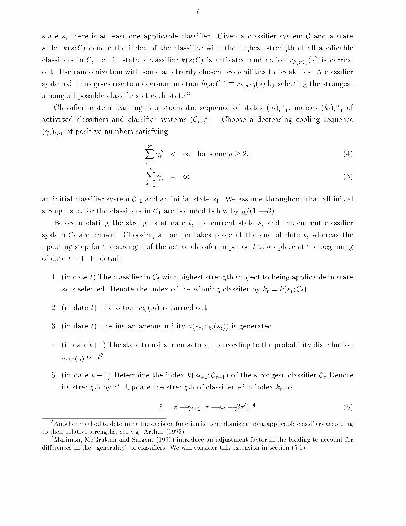
7state s, there is at least one applicable classi�er. Given a classi�er system C and a states, let k(s; C) denote the index of the classi�er with the highest strength of all applicableclassi�ers in C, i.e. in state s classi�er k(s; C) is activated and action rk(s;C)(s) is carriedout. Use randomization with some arbitrarily chosen probabilities to break ties. A classi�ersystem C thus gives rise to a decision function h(s; C ) � rk(s;C)(s) by selecting the strongestamong all possible classi�ers at each state.3Classi�er system learning is a stochastic sequence of states (st)1t=1, indices (kt)1t=1 ofactivated classi�ers and classi�er systems (Ct)1t=1. Choose a decreasing cooling sequence( t)t�0 of positive numbers satisfying1Xt=1 pt < 1 for some p � 2; (4)1Xt=1 t = 1 (5)an initial classi�er system C 1 and an initial state s1. We assume throughout that all initialstrengths zc for the classi�ers in C1 are bounded below by u=(1 � �).Before updating the strengths at date t, the current state st and the current classi�ersystem Ct are known. Choosing an action takes place at the end of date t, whereas theupdating step for the strength of the active classifer in period t takes place at the beginningof date t+ 1. In detail:1. (in date t) The classi�er in Ct with highest strength subject to being applicable in statest is selected. Denote the index of the winning classifer by kt = k(st; Ct).2. (in date t) The action rkt(st) is carried out.3. (in date t) The instantaneous utility u(st; rkt(st)) is generated.4. (in date t+1) The state transits from st to st+1 according to the probability distribution�st;r(st) on S .5. (in date t + 1) Determine the index k(st+1; Ct+1) of the strongest classi�er Ct Denoteits strength by z0. Update the strength of classi�er with index kt to~z = z � t+1 (z � ut � �z0) :4 (6)3Another method to determine the decision function is to randomize among applicable classi�ers accordingto their relative strengths, see e.g. Arthur (1993).4Marimon, McGrattan and Sargent (1990) introduce an adjustment factor in the bidding to account fordi�erences in the \generality" of classi�ers. We will consider this extension in section (5.1).

8The classi�er system Ct+1 is then de�ned to be the classi�er system Ct with c replacedby ~c = (r; ~z).The updating of the strength of the classi�er activated in period t occurs at stage 5 whenut and st+1 are known. Note, that the updating equation (6) uses the period t strenghts todetermine z0 which is added to the strength of classi�er which is active in period t. After�nishing with stage 5, we go on to stage 1 in time t + 1. The classi�er chosen at stage 1in period t + 1 might di�er from the \hypothetical" one which was used to complete theupdating in stage 5. The updating algorithm is formulated in such a way that the updatingdoes not require calculating the strengths at t + 1 �rst, which would otherwise give rise tocomplications in cases where the activated classi�ers at date t and t+1 have the same index.This is an attractive way to model boundedly rational learning since it relies only on simplecalculations and avoids complex forward-looking reasoning like forming expectations.The strength updating equation (6) is often referred to as a bucket brigade, since eachactivated classi�er has to pay or give away part of its strength z in order to get activated, butin turn receives not only the instantaneous reward ut for his action, but also the \payment" bythe next activated classi�er �z0, discounted with �. Note the formal similarity to equation (1)which hints at the intuition why the bucket brigade is able to deal with the dynamic structureof the maximization problem. Numerical procedures to calculate the value function in (1)are often based on iterations of approximation of the value function. A guess is pluggedinto the right hand side of (1) which yields a new guess. The new guess is in turn pluggedinto the right hand side, and so on. The contration mapping theorem ensures that thisprocess converges to the true value function. The bucket brigade algorithm accomplishes asimilar approximation for the strengths of the classi�ers instead of the state dependent valuefunction.We should stress that an agent who is equipped with a classi�er system only performsvery simple computations. She does not have to deal with a complex dynamic programmingproblem but learns via the simple bucket brigade algorithm for updating the strenghts.Moreover, she only has to memorize K numbers, the strength for each classi�er, which forlarge state spaces might be much smaller than the number of states n. The dimension ofthe value function in the dynamic program is of course equal to n. Note, however, that thenumber of classifers can in general be larger than the number of states.

94 Asymptotic BehaviorClassi�er system learning leads to a stochastic sequence of decision functions (ht)1t=1 given byht = h(st; Ct). We are interested in determining the asymptotic behavior of this sequence, i.e.which decision functions are eventually learned, and whether they coincide with an optimaldecision function for (1).It is convenient for the further analysis to rewrite the accounting scheme (6) as a stochas-tic approximation algorithm in the following way (for a general overview and introduction tostochastic approximation algorithms, see Sargent (1992) and Ljung, P ug and Walk (1992)). 5Let �t be the K-dimensional vector of all strengths at date t. Let Yt = [st�1; kt�1; st; kt] be thevector of the past and present state and the indices kt�1 and kt of the activated classi�ers.Given Yt and �t, the updating procedure as laid out above generates Yt+1. The vector �t+1is computed via �t+1 = �t � t+1f(�t; Yt+1) (7)with f(�t; Yt+1) = ekt g(�t; Yt+1); (8)where ekt is the K-dimensional unit vector with a one in entry kt and zeros elsewhere, andwhere g(�t; Yt+1) = �t;kt � u(st; rkt(st))� ��t;kt+1: (9)Note that f is linear in �t. Furthermore, if u=(1 � �) � �t;k � �u=(1 � �) + �� for all k andsome �� � 0, then u=(1 � �) � �t+1;k � �u=(1 � �) + ��� for all k. Thus, the elements of �twill be bounded below and above by u=(1 � �) and �u=(1 � �) in the limit as t ! 1. Thesequences (�t;k)t are in general not monotonically decreasing, even if the starting strengthszk of the �rst classi�er system C1 are bounded below by �u=(1 � �), but they are typicallyclose to being monotonically decreasing in numerical applications.Consider a vector of strengths �1 so that, conditional on some strength �t0 and somevalue for Yt0 at some date t0, we have �t ! �1 with positive probability. If all elementsof �1 are distinct, we call �1 a limit strength vector. We aim at characterizing all limitstrength vectors. To do that, we �rst consider a special situation and formulate necessaryconditions for a vector to be a limit strength vector in that situation, see Proposition 2 andthe consistency condition below. We then show in Theorem 1, that these conditions are acomplete characterization in general.5Marimon et. al. (1990, sec. 5) already suggest to use stochastic approximation results to study the limitbehavior of classi�er system.

10Consider the special situation where convergence to �1 is almost sure for any value ofYt0, and where the ordering of the elements in �t coincides with the ordering of the entriesin �1 almost surely for all t � t0. Using the list of rules from the classi�er system C1and attaching strengths according to a strength vector � 2 IRK allows one to identify astrength vector � with a classi�er system C�. Given a limit strength vector �1, �nd theassociated classi�er system C1. Find the index k(s) = k(s; Ct) of the strongest classi�er foreach state s, the resulting decision function h(s) = h(s; Ct), the associated transition matrix�h and thus the invariant distribution �h on S . Note that k(s) coincides with k(st; Ct) forall t � t0 almost surely by our special assumption. Thus, the transition law for the statevector Yt to Yt+1 can be restated as drawing st+1 according to the transition law �h andsetting the index kt+1 to be the index k(st+1): denote this transition law with �̂. Since�h is the unique invariant distribution for �h, it follows that there is a unique invariantdistribution � for �̂. The marginal distribution of � with respect to the index kt in Yt+1yields an invariant distribution � on the set f1; : : : ;Kg of classi�er indices. This distributioncan alternatively be computed directly via �(k) = Prob(k = k(s)) = Pfsjk=k(s)g �h(s). Callclassi�ers asymptotically active if they are a winning classi�er for at least one state, i.e. if�(k) > 0. Call all other classi�ers asymptotically inactive. De�ne�(�) � E� [f(�; Y )] ;where the expectation is calculated with respect to the invariant distribution �.Proposition 2 In the special situation where convergence to �1 is almost sure for anyvalue of Yt0, and where the ordering of the entries in �t coincides with the ordering of theentries in �1 almost surely for all t � t0, a necessary condition for a limit strength vector is�(�1) = 0: (10)Proof: Take expectations with respect to the invariant distribution � over the initialstate Yt0 in equation (7) and sum from t = t0 to some T . Since � is the invariant distribution,this amounts to taking expectations with respect to the invariant distribution over each futureYt as well. Exploiting almost sure convergence yields�1 = �t0 � 1Xt=t0 t+1�(�t): (11)Assume now that (10) does not hold and that instead, say, �(�1) > � > 0. Since �(�t) !�(�1) and hence �(�t) > �=2 for t � T , some T , a contradiction follows from (11), (5) andthe �niteness of �1. �

11The necessary condition (10) can be studied a bit further. It is easy to see that�(�) = � � (� � ~u� �B�) ; (12)where � denotes element-by-element multiplication of two vectors of equal dimension, where~u = 266664 ...E�h [u(s; rk(s)) j k(s) = k]... 377775 (13)(and arbitrary entries, whenever the conditional expectation is not well de�ned, i.e. whenever�(k) = 0) and where B is a matrix withBk;l = Prob(fs0 j k(s0) = lg j k(s) = k)= Pfijk=k(si)gPfjjl=k(sj)g �h(si)�h;i;j�(ck) (14)for all indices k indexing classi�ers with �(k) 6= 0 (choose some arbitrary number between 0and 1 otherwise).Suppose one were given only the ordering of the classi�ers according to �1 rather thanthe strength vector itself. Given the ordering, one can recover the index of the winningclassi�er k(s) as well as the decision function h, the utilities u(s; rk(s)) and the probabilities�h;i;j, �h(s) and �(k). Equation (10) can thus be used to solve for �1 by solving a systemof K linear equations in K unknowns. For the asymptotically active classi�ers, a simplecontraction mapping argument shows that their strengths is uniquely given by�1 = (I � �B)�1~u; (15)where (in slight abuse of notation) the rows and columns corresponding to asymptoticallyinactive classi�ers are meant to be eliminated in that equation. Equation (10) does notimpose any restrictions on the strength of asymptotically inactive classi�ers. However theirvalue can be bound by inspecting the construction of k(s) from the ordering implied by �1:the strength of any classi�er, including asymptotically inactive classi�ers, is bound aboveby the strengths of the asymptotically active classi�ers which are applicable in states wherethe given classi�er is applicable as well. In other words, the following consistency conditionapplies.consistency condition:for all s 2 S and all classi�ers ck in C� with k 6= k(s) and c(s) 6= a0, we have�1;k < �1;k(s).

12We call a vector �1 2 IRK a candidate limit strength vector, if �1 satis�es equation (10)as well as the consistency condition. Note that the calculations leading up to and following(10) essentially only require knowledge of the ordering of the classi�ers resulting from �1.As a result of the discussion above we thus haveProposition 3 1. Under the conditions of proposition 2, every limit strength vector isa candidate limit strength vector.2. For each of the K! possible strict orderings of the K classi�ers, there is a vector �1 2IRK satisfying (10). �1 is unique up to the assignment of strengths to asymptoticallyinactive classi�ers. �1 is a candidate limit strength vector, if it satis�es the consistencycondition.It is important when interpreting the second part of this proposition, that the givenordering of the classi�ers is used to calculate k(s), not the solved-for strength vector �1, andthe resulting decision function and probabilities. The vector �1 may give rise to a di�erentindex ~k(s) of the winning classi�er and it is the task of the consistency condition to checkfor the equality of k(s) with ~k(s).For two special cases, the candidate limit strength vectors are easy to construct and aredirectly related to the dynamic programming calculations in section 2.Proposition 4 Suppose there is only one rule r 2 R . Then there is a unique candidatelimit strength vector �1 2 IR and it satis�es � = E�rvr. In particular, if r = h�, then�1 = E�h�v�.Proof: In this case (15) reduces to�1 = (I � �)�1E�h[uh]: (16)We therefore need to show that E�h[vh] = (1� �)�1E�h[uh] (17)or (1� �)�Tvh = �huh: (18)But this follows immeadiately from (3) and from the fact that�T = �T�h; (19)

13which completes the proof. �However, in general zk 6= E�h [vh(s)jk(s) = k] : (20)Proposition 5 Let h� be a decision function with v� = vh� and suppose that h� is unique.Suppose, furthermore, that all K rules are applicable in at most one state and that for eachs 2 S , there is exactly one rule with r(s) = h�(s); denote its index with k�(s). De�ne �by assigning for each state s strength v�(s) to the classi�er with index k�(s). For all otherclassi�ers c applicable in some state s, assign some strength strictly strictly below v�(s).Then �1 is a candidate limit strength vector which implements the dynamic programmingsolution.Proof: Compare equation (15) to equation (3) and note that B = �h and ~u = uh. �Theorem 1 shows that our characterization is general.Theorem 1 Every candidate limit strength vector is a limit strength vector and vice versa.The proof of this theorem can be found in Appendix A. It draws on a result by Metivierand Priouret (1984) about Markov stochastic approximation procedures, restated in Ap-pendix B for convenience. The theorem indicates how classi�er system learning happensover time. For some initial periods, the orderings of the classi�ers may change due to chanceevents. Eventually, however, the system has cooled down enough and a particular orderingof the strengths is �xed for all following periods. As a result, the asymptotically inactiveclassi�ers will no longer be activated, and the system converges to the limit strength vectoras if the transition from states to states was exogenously given: the classi�er system haslearned the �nal decision rule. Alternatively, one can train a classi�er system to learn aparticular decision rule corresponding to some candidate limit strength vector by forcing theprobabilistic transitions from one state to the next to coincide with those generated by thedesired decision rule: after some initial training periods, the strengths will remain in thedesired ordering and will not change the imprinted pattern. The number of initial trainingperiods and the number of the cooling periods is path-dependent; however, given a particularhistory, the theorem and its proof do not rule out that the strengths break free once moreto steer towards a di�erent limit. In fact, this will typically happen with some probability

14due to (5). If there is a su�ciently long string of \unusual events", these events can have alarge e�ect on the updating of the strengths in (6) and thus change an existing ordering.It should be noted that the characterization only applies to limit strength vectors witha strict ordering of the strengths. As we will see in the next section, this is not just rulingout knife-edge cases. A robust example will be constructed, where equality of the strengthsof two classi�ers is necessary asymptotically.5 ExamplesWe provide an example which demonstrates the similarities and the di�erences betweenclassi�er systems and the dynamic programming approach. It also demonstrates why thecase of several asymptotically active classi�ers for one state cannot be ruled out. The exampleis abstract and meant for illustration only; it has therefore been kept as simple as possible.Suppose S = f1; 2; 3g, A = f1; 2g and that the transition to the next state is determinedby the choice of the action only, regardless of the current state s:s0 = 1 s0 = 2 s0 = 3a = 1 : �s;1(1) = 1=3 �s;1(2) = 1=3 �s;1(3) = 1=3a = 2 : �s;2(1) = 0 �s;2(2) = 1 �s;2(3) = 0Note, that some probabilities are zero, in contrast to our general assumption. This is doneto simplify the algebra for this example. We further have a discount factor 0 < � < 1 andutilities u(s; a); s = 1; 2; 3; a = 1; 2. We assume without loss of generality that u(2; 1) = 0.We impose the restriction that u(3; a) = u(1; a) for a = 1; 2, so that state s = 3 is essentiallyjust a \copy" of state s = 1. Thus, there are three free parameters, u(1; 1), u(1; 2) andu(2; 2).The di�erence between state s = 1 and state s = 3 is in how they are treated by theavailable rules. Assume that there are two rules, r1 and r2, described byr1 r2s = 1 : r1(1) = 1 r2(1) = 2s = 2 : r1(2) = 0 r2(2) = 1s = 3 : r1(1) = 1 r2(1) = 0with \0" denoting the action a0, i.e. non-applicability. Note that rule 2 is applicable in states = 1 but not in state s = 3.We aim at calculating all candidate limit strength vectors. Since there are only tworules, there can be only two strict rankings of the corresponding classi�er strengths, namely

15z1 > z2 (Case I) and z2 > z1 (Case II). We will also have reason to consider the case z1 = z2with nontrivial randomization between the classi�ers (Case III), a situation not covered byour theoretical analysis above. Each of these cases are analyzed below. Note that the twogiven rules never lead to action a = 2 in state s = 2: the value of u(2; 2) is thus irrelevantfor the comparison of the classi�ers. Each of the cases below will thus be valid only undersome restrictions on the values for the remaining two free parameters u(1; 1) and u(1; 2).The results are summarized in Table 1 and Figure 1.Case I: z1 > z2: In this case, classi�er 1 is activated in states s = 1 and s = 3 and classi�er2 is activated in state s = 2. Thus, action a = 1 is taken in all three states: h(s) � 1.It follows that �h(1) = �h(2) = �h(3) = 1=3. For the strengths, one needs to solve theequations z1 = u(1; 1) + �3 (2z1 + z2)z2 = �3 (2z1 + z2):This case can thus be obtained if and only ifu(1; 1) > 0: (21)Case II: z2 > z1: In this case, rule 2 is applied in states s = 1 and s = 2 whereas rule1 is applied in state s = 3. Hence, h(1) = 2; h(2) = 1; h(3) = 1 and consequently�h(1) = �h(3) = 1=4 and �h(2) = 1=2. The strengths are calculated fromz1 = u(1; 1) + �3 (z1 + 2z2)z2 = 13(u(1; 2) + �z2) + 2�9 (z1 + 2z2):It is easily checked that this case can be obtained if and only ifu(1; 2) > 3u(1; 1): (22)Case III: z1 = z2 = z: . We provide a \solution" for this case, even though our theory abovedoes not cover cases without strict ranking of the classi�ers. The reasoning employedhere should be rather intuitive, however. Given state s = 1, we guess that classi�er c1is activated with some probability p, whereas classi�er c2 is activated with probability 1- p, i.e. there is randomization between the classi�ers. The resulting decision functionis random. Given s = 1, states s0 = 1 and s0 = 3 will be reached with probability

16p=3 each. The invariant distribution �h is therefore �h(1) = �h(3) = 1=(4 � p),�h(2) = (2 � p)=(4 � p). Let �h(s; k) be the joint probability that state s occursand classi�er k is activated. We havec1 c2s = 1 : �h(1; 1) = p=(4 � p) �h(1; 2) = (1� p)=(4 � p)s = 2 : �h(2; 1) = 0 �h(2; 2) = (2� p)=(4 � p)s = 3 : �h(3; 1) = 1=(4 � p) �h(3; 2) = 0:The common strength z should satisfy both equations arising from (10), one for clas-si�er c1 and one for classi�er c2 yielding11 � �u(1; 1) = z = 11 � � 1 � p3� 2pu(1; 2); (23)which can be solved for p. Note that p is a viable probability if and only if 0 � p � 1.Thus, case III is valid, if and only if one of the following two inequality restrictions issatis�ed:� u(1; 2) � 3u(1; 1) � 0 or� u(1; 2) � 3u(1; 1) � 0.The calculated strengths and probabilities calculated in this case are unique except ifu(1; 1) = u(1; 2) = 0. The inequalities have to be strict in order for p to be nontrivial:otherwise, the decision rule obtained coincides with the one derived from case I or caseII.Table 1 shows that for any given values of u(s; a) there is at least one applicable case.However, the only case available may be Case III and thus the solution prescribed by theclassi�er system involves randomizing between the classi�ers.It is interesting to compare these possibilities with the solution to the dynamic program-ming problem. If u(2; 2) is large enough, the optimal decision function will always prescribeaction a = 2 in state s = 2, which cannot be done with the classi�ers above. Any classi�ersystem with the rules given above will result in a suboptimal solution simply because thecorrect solution is not within reach.Assume instead that u(2; 2) is small enough, so that the decision function h� solvingthe dynamic programming problem takes action h�(2) = 1 in state s = 2. By symmetry,h�(1) = h�(3) and v�(1) = v�(3). Furthermore, h�(1) = h�(3) = 1 if and only ifu(1; 1) + �=2 (v�(1) + v�(2)) � u(1; 2) + �v�(2) (24)

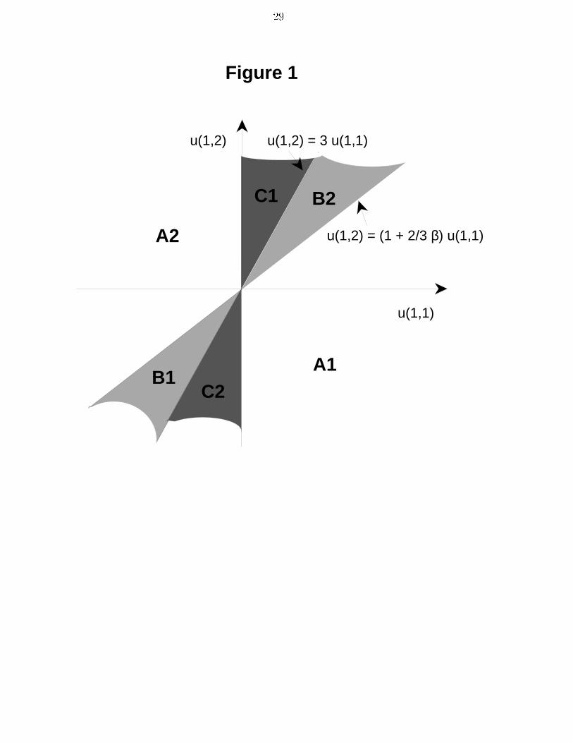
17and h�(1) = 2 otherwise.6 Directly calculating v� = vh� with equation (3) for the two choicesyields� h�(1) = 1, if u(1; 2) � �1 + 23��u(1; 1),� h�(1) = 2, if u(1; 2) � �1 + 23��u(1; 1).A summary of all possible situation is found in Table 1 and Figure 1. The learnabledecision function may not be unique (area C2). The learnable decision function may involveasymptotic randomization between the available rules (area C1). The learnable decisionfunction can also be di�erent from the solution to the dynamic programming problem, evenif that solution is attainable by ranking the classi�ers appropriately: this is the case in areaB1. The intuitive reason for this last observation is quickly found: since u(2; 1) has beennormalized to zero, u(1; 1) measures how much classi�er c1 gains against classi�er c2 by beingapplicable in state 2 rather than state s = 1. If u(1; 1) is positive, state s = 3 correspondsto \good times" and state s = 2 corresponds to \bad times". Since the accounting systemfor calculating the strength of classi�ers does not distinguish between rewards generatedfrom the right decision and rewards generated from being in good times, a classi�er that isapplicable only in good times \feels better" to the arti�cially intelligent agent than it should.Thus, if u(1; 1) > 0, classi�er c1 may be used \too often" and if u(1; 1) < 0, classi�er c1 maybe used \too little". This is what happens in regions B and C.5.1 Adjusting for GeneralityIn the bidding and accounting scheme as laid out in section (3) each classi�er is treatedequally independent of their generality. The example above shows that rules which areapplicable only in a small number of states, ie. speci�c rules, can dominate \better" generalrules even if their are inferior. This raises the immediate question whether it is possibleto adjust the scheme so that this drawback can be eliminated. Marimon, McGrattan andSargent (1990) adjust the payment of the classi�ers with a proportional factor that dependson the number of states in which the classi�er is active. We will allow for the more generalcase where there is a general correction factor for each classi�er.Consider the above example with only two classi�ers. Let �1; �2 be the adjustment factorfor the classi�er 1 and 2, respectively and let xi = �izi be the adjusted strength for classi�eri. The �rst obvious change in the scheme is as follows. The strongest classi�er is foundby comparing the values of �z instead of just z and the strength is updated according to6If equation (24) holds with equality, both choices for h�(1) are optimal.

18~z = z � t+1 (�z � ut � ��0z0) : However, the di�erence to the accounting system presentedabove is small and immaterial asymptotically. To see that rewrite the equation as ~x =x � � t+1 (x� ut � �x0) and therefore di�ers from (6) only by a classi�er-individual scalaradjustment for the updating step size. Asymptotically, only the expression in bracketsmatters, and there is no di�erence. This shows that for the adjustment to work in the limit,one has to distinguish between the bidding and the payment between the classi�ers. Thuswe propose the following adjustment.The bid of each applicable classi�er is still equal to its strength. Thus the strongestclassi�er still wins the bidding. However, the winning classi�er only pays back x = �zinstead of z. Hence, the adjustment factors � determine how much of its strength the winningclassi�er has to give away. A classi�er with a low � has thus an advantage over a classi�erwith a high �. Next we check whether it is possible to �nd a set of �'s which guaranteethat the classi�er learning solution is identical to the dynamic programming solution. Wenormalize �2 to unity thus leaving �1 as free parameter. Assume for the moment that thedynamic programming solution prescribes h�(1) = 1 (the condition for this case is given inthe preceeding section). Thus, we have to �nd �1 so that classi�er 1 is stronger than classi�er2 in the limit, ie. z1 > z2. Note that since the payments are now x1 and x2, equation (10) x2.Using x1 = �1z1 and x2 = z2 we can get the consistency condition in terms of the strengths.We get z1 � z2 = u(1; 1) " 3��� � 2�3(1� �) # : (25)Hence, if u(1; 1) > 0 any � satisfying � < 3� �2� (26)will give the desired result that classi�er 1 is stronger than classi�er 2. If u(1; 1) < 0 theinequality is reverses. The analysis for the other case z2 > z1 is analogous. This showsthat we always can �nd appropriate payment adjustments that can lead the classi�er systemsolution to coincide with the dynamic programming solution if it is attainable. Note however,that this is only possible after having solved the dynamic program. In other words, it is notpossible to select the correct payment adjustment factors without knowing the dynamicprogramming solution.7Furthermore, it is not clear whether letting the adjustment parameters depend on thegenerality of the classi�ers is optimal in every case. It might solve the problem of selecting7Marimon, McGrattan and Sargent's \bids" correspond to our payment �z. The winning classi�er intheir paper is, as in ours, determined by the strength and not by the as bid, as one might be led to believefrom their teerminology. From this it follows that more general rules bene�t from their adjustment schemeand not speci�c ones as they say on p. 338.

19inferior speci�c rules in some cases. But one also could imagine cases where a speci�c butsuperior rule which is only applicable in bad states s dominated by an general but inferiorrule which is applicable in good and bad states. Instead one could de�ne adjustment schemeswhich depend on whether a classi�er is applicable in \good" or in \bad" states. In general,the above analysis shows that rules that are applicable in \good" states should receive ahigh � thus penalizing them for being applicable in these good times. On the contrary,classi�ers which are mostly applicable in bad states should receive a low �. Of course, insome problems it is ex ante not clear to determine which state is \good" and which one is\bad". In these cases it is hard to �nd suitible adjustment parameters.6 Generating Excess Sensitivity of Consumption toTransitory IncomeConsider the puzzle of excess sensitivity of consumption to transitory income as documentedby Hall and Mishkin (1982), Zeldes (1989) and Carroll and Summers (1991) among others.DeLong and Summers (1986) and Campbell and Mankiw (1989, 1991) propose ad hoc ruleof thumb consumers to explain this feature of aggregate consumption. Their rule of thumbconsumers are not as sophisticated as our learning agents. They estimate models which allowfor a �xed proportion of consumers who just consume their current income and �nd that thespeci�cation including rule of thumb consumers is capable of producing excess sensitivity. Inan alternative approach Laibson (1993) explains the puzzle as stemming from the inabilityto precommit future selves not to spend too much out of transitory income.We will construct an example to show that classi�er system learning can generate suchbehavior even if the optimal decision function is part of the system since bad decisions ingood times can \feel better" than good decisions in bad times. Speci�cally we show that thead-hoc rule of thumb \consume current income" can be the asymptotic outcome of classi�ersystem learning. In order to get analytical results we make some simplifying assumptions,but the general avor of the results should be intuitive even in more complex models.There is an in�nitely lived agent who derives utility u(ct) from consuming in period tand who discounts future utility at the rate 0 < � < 1. The agent receives random incomeyt each period. Suppose there are two income levels, y > y > 0 and that income follows aMarkov process with transition probabilities py y = Prob(yt = y j yt�1 = y), etc.. The agententers period t with some wealth wt. Next periods wealth is given by wt+1 = wt + yt � ct.A borrowing constraint is imposed so that ct � wt + yt. Furthermore, we assume that theagent is born with zero wealth: w0 = 0.

20To cast this model into our framework, we discretize the model and assume that allvariables take only integers values: w 2 f0; 1; 2; : : : ; �wg, etc.. The state of the system isgiven by st = (wt; y), where y is the present income level, y 2 fy; yg. Note that the impliedtransition probabilities �ij from state i to state j are not strictly positive, in contrast to ourassumption in section 2. This assumption is for simpli�cation of the algebra only. 8The dynamic programming problem is given byv(w; y) = maxc2f0;1;:::;w+yg0B@u(c) + � Xy02fy;yg pyy0 [v(w+ y � c; y0)]1CA : (27)Given particular choices for the (increasing) utility function and the parameters of thismodel, this dynamic programming problem can be solved with the techniques in section 2.Let h�(s) = c�(w; x) be the decision function solving this dynamic program. Note thatc�(0; yl) = y. Hence when the agent has zero wealth and current income is low, she spendsall her income.Now consider two rules, r1 and r2 with strengths z1 and z2 respectively. Rule r1 isapplicable in all states and coincides with the optimal decision function h�. Rule r2 isapplicable only in states when the income is high, i.e. in \good" states. We assume thatr2(w; y) = w + y; (28)so that rule r2 prescribes consumption of the maximal amount when income is high.Will the suboptimal rule r2 be asymptotically active when it is applicable despite thefact that the optimal rule r1 is always applicable? This coincides with the ranking z2 > z1.Note that in this regime the agent always spends her total current income and never savesThis is the ad-hoc rule of thumb consumer considered by DeLong and Summers (1986) andCampbell and Mankiw (1989, 1991). Thus the invariant distribution over states �h haszero weight on all states st = (w; y) with w > 0; y 2 fy; yg. This makes the equation forcalculating the strengths very simple:z1 = u(yl) + �(py yz1 + (1� py y)z2) (29)z2 = u(yh) + �(py yz1 + (1� py y)z2): (30)Solving these two equations for z1 and z2 gives the limit strengths. To see whether this8We could modify the model in the following way so that �ij > 0 8i; j. Let p > 0 be the probability thatnext periods wealth is given by wt+1 = wt+ yt� ct whereas with probability 1� p, an arbitrary wealth levelwt+1 is drawn next period uniformly from 0; 1; :::; �w. While all the results are valid for p close to unity, thealgebra is much more cumbersome. For simplicity we choose p = 1.

21ranking is feasible we have to check if z2 > z1 sincez2 � z1 = u(y)� u(y)1� �(py y � py y) > 0; 0 < py y; py y; � < 1; (31)rule r1 (r2) will be active when income is low (high). The resulting consumption decisionis h(s) = c(w; y) = y. The intuition behind this suboptimal behavior is as in the precedingexample: rule r2 may be asymptotically stronger than rule r1 since it only applies in \goodtimes" and thus \feels better" on average than rule r2. Thus we have demonstrated that ruleof thumb consumption behavior can be the outcome of learning behavior and thus shouldnot be dismissed as completely ad-hoc.This example is only intended as an illustration. We should stress that the choice ofclassi�ers is ad hoc. However, the resulting behavior should be fairly robust in more complexproblems.7 ConclusionIn this paper we have discussed the asymptotic behavior of rules of thumb learning repre-sented by Holland's (1986) classi�er system. We have shown how a bucket brigade algorithmenables classi�er systems to deal with general discrete recursive stochastic dynamic optimiza-tion problems. We reformulated the evolution of the strengths as a stochastic approximationalgorithm. Using a theorem by Metevier and Priouret (1984) we are able to obtain a gen-eral characterization of all possible limit outcomes provided that the classi�ers are strictlyordered in the limit. A simple example shows that the attainable decision function is neithernecessarily unique nor characterized by a strict ordering of classi�ers. With these resultswe are also able to compare classi�er learning to the dynamic programming solution of thedynamic optimization problem. Due to the bucket brigade payment scheme, the classi�erstrengths are in close relationship to the value function of the dynamic problem, in fact, incertain situations they coincide.The example also shows in what circumstances classi�er system learning may lead tosuboptimal behavior even when the optimal decision rule is an element of the classi�ersystem. Since the optimal classi�er is applicable in all possible states of nature, a suboptimalclassi�er might dominate the optimal one if is applicable only in \good" states of the world.Bad decisions in good times can \feel better" than good decision in bad times. We also showthat this e�ect might lead a consumer in an intertemporal consumption problem to consumetoo much in periods of high income generating excess sensitivity to transitory income.

22AppendixA Proof of Theorem 1Proof: We �rst show that a given candidate limit strength vector is a limit strengthvector. To that end, we analyze �rst an alteration of the stochastic approximation schemeabove and characterize its limits in the claim below. We then show that the limit to thisaltered scheme corresponds to a limit strength vector in the original scheme.Claim: Consider a candidate limit strength vector �1a and its associated decisionfunction h. Fix the transition probabilities �h. Consider the following altered updatingsystem: let the classi�er system consist only of the asymptotically active classi�ers accordingto �1. Fix some starting date t0, initial strength vector �t0 with �t0;l � u=(1 � �) for all land an initial state Yt0 . Let ~�t be the vector of strengths of this reduced classi�er systemat date t � t0 and let ~�1 be the corresponding subvector of �1 of strengths of only theasymptotically active classi�ers. Furthermore, let the transition from state st to st+1 alwaysbe determined by the transition probabilities �h. Then ~�t ! ~�1 almost surely. Furthermore,for almost every sample path, the transition probabilities �st;rkt coincide with the transitionprobabilities given by �h for all but �nitely many t.Proof of the Claim: The updating scheme is still given by (7), (8) and (9). Thetransition law for Yt is given by �̂, where �̂ was de�ned in section 4. In particular, �̂ doesnot depend on ~�t due to our alteration of the updating process. The random variables Y liein a �nite, discrete set. Note that ~�t always remains in the compact set � = [u=(1� �); �z]d,where d is the number of asymptotically active classi�ers and �z is the maximum of all initialstarting strengths in ~�t0 and �u=(1 � �). With our remarks after theorem 2 in Appendix B,this theorem thus applies if we can verify assumptions (F), (M1), (M5c) and the additionalassumptions listed in the theorem itself.Assumption (F) is trivial, since f is continuous. Assumption (M1), the uniqueness of �,follows from the uniqueness of �h. For (M5c), note that I � �̂ is continuously invertible onits range and that f(~�; Y ) is linear and thus Lipschitz continuous in ~�. For the additionalassumptions of the theorem, note �rst that p =1 in (M2) is allowed according to our remarksfollowing the theorem in Appendix B, so that the restriction Pn 1+(p=2)n <1 is simply therestriction that the sequence ( n) is bounded. For the conditions on the di�erential equation,consider � as given in equation (12) and ~u and B given in equations (13) and (14) restrictedto entries of asymptotically active classi�ers. Note that the di�erential equation

23d~�(t)dt = ��(~�(t))= � � �~�1 � ~u� �B~�1�is linear with the unique stable point ~� given by (15). The di�erential equation is globallystable since the matrix �� � (I � �B) has only negative eigenvalues (note that 0 < � < 1and that Bk;l is a stochastic matrix). Theorem 2 thus applies with A = � and we havelimt!1 ~�t = ~�1 a.s.,as claimed.The claim that the transition probabilities �st;rkt coincide with the transition probabil-ities given by �h follows from the almost sure convergence to the limit. Given almost anysample path, all deviations ~�t;k� ~�1;k will be smaller than some given � > 0 for all t � T forsome su�ciently large T, where T depends in general on the given sample path and on �.Make � less than half the minimal di�erence between the limit strengths of any two di�erentclassi�ers j ~�1;k � ~�1;l j. We then have that the ranking of the classi�ers by strength willnot change from date T onwards. But that means that the transition probabilities �st;rktcoincide with the transition probabilities given by �h, concluding the proof of the claim. �Given a candidate limit strength vector �1, �nd � > 0 such that 4� is strictly smallerthan the smallest distance between any two entries of �1. Denote the underlying probabilityspace by (;�;P) and states of nature by ! 2 . Consider the altered updating scheme asdescribed in the claim above with t0 = 1 and the given initial state. Find the subvector ~�1of �1, corresponding to the asymptotically active classi�ers according to �1. We can thus�nd a date t1, a state Y and a strength vector �� for only the asymptotically active classi�ersso that given some event 0 � of positive probability, sample paths satisfy Yt1 = Y ,j ~�t1;l � ��l j< � for all l, j ~�t;l� ~�1;l j< � for all l and all t and ~�t ! ~�1. For any sample path(~�t)t�t1 (i.e. not just those obtained for states of nature in 0) , �nd the \shifted" samplepath (�̂t)t�t1 obtained by starting from �̂t1 = �� instead of ~�t1, but otherwise using the samerealizations ut and states Yt for updating. This resets the initial conditions and shifts thestarting date to t1, but leaves the probabilistic structure otherwise intact: the claim thusapplies and we have again �̂t ! ~�a.s.. Furthermore, given 0, an induction argument appliedto (6) yields j �̂t;l� ~�t;l j�j �̂t1;l� ~�t1;l j< � for all t � t1 and all l. As a result, j �̂t;l� ~�1;l j< 2�for all t � t1 and all l, given 0. Extend �̂t to a strength vector ��t for all classi�ers byassigning the strengths given by �1 to inactive classi�ers. By our assumption about �, the

24ordering of the strengths given by any ��t, t � t1 coincides with the ordering of the strengthsgiven by �1. Thus starting the classi�er system learning at t1, strength vector �t1 = ��t1 andstate Yt1 = Y at t1, the evolution of the strengths �t is described by �t = ��t for all ! 2 0and we therefore have that �t ! �1 with positive probability. This shows that �1 is a limitstrength vector, completing the �rst part of the proof.Consider in reverse any limit strength vector �1: we have to show that �1 satis�es (10),since the consistencyconsistencyconsistencyconsistency condition is trivially satis�ed by def-inition of k(s). Find � > 0 so that 4� is strictly smaller than the smallest distance betweenany two entries of �1. Find a date t1 � t0 so that on a set 0 of positive probability, we havej �t;l��1;l j< � for all t � t1 and all l, and �t ! �1. Given the strict ordering of the strengthsin �1, there is a candidate limit strength vector �01 which is unique up to the assignment ofstrength to asymptotically inactive classi�ers, see proposition 3. Given any particular stateof nature �! 2 0 and thus values for �t1 and Yt1 at date t1, consider the altered updatingscheme as outlined in the claim with that starting value (and t0 � t1 for the notation in theclaim). Via the claim, ~�t ! ~�1 a.s., where ~�01 is the subvector of the candidate limit strengthvector �01 corresponding to the asymptotically active classi�ers. Thus, the strengths in ~�(!)coincide with the strengths of the asymptotically active classi�ers in �t(�!) for almost all !and it is now easy to see that therefore the strengths of the asymptotically active classi�ersin �1 has to coincide with the strength of the asymptotically active classi�ers in �01, �nishingthe proof of the second part. To make the last argument precise, observe that ~�t(!) ! ~�1except on a measurable nullset ! 2 ��! 2 �. Note that the exceptional set is the samewhenever the initial conditions �t1 and Yt1 are the same. Since there are only �nitely manysuch initial conditions that can be reached, given the discrete nature of our problem andthe �xed initial conditions at date t0, the exceptional set � = f(�!; !) j �! 2 0; ! 2 ��!g is ameasurable subset of zero probability of 0 � in the product probability space on � .It follows that the strengths of the asymptotically active classi�ers in �1 and �01 coincidefor all (�!; !) 2 0�=�, which is a set of positive probability. Since these strengths are notrandom, we must have equality with certainty. �

25B A Theorem about Markov Stochastic Approxima-tion AlgorithmsIn this section, we use the notation of Metivier and Priouret (1984). For a general overviewand introduction to stochastic approximation algorithms, see Sargent (1992) and Ljung,P ug and Walk (1992).For each � 2 IRd consider a transition probability �̂�(y; dx) on IRk. This transitionprobability de�nes a controlled Markov chain on IRd.De�ne a stochastic algorithm by the following equations:9�n+1 = �n � n+1f(�n; Yn+1) (32)where f(�; y) is a function f : IRd � IRk ! IRd,P [Yn+1 2 B j Fn] = �̂�n(Yn;B) (33)where P [Yn+1 2 B j Fn] is the conditional probability of the event fYn+1 2 Bg given �0; : : : ; �n,Y0; : : : ; Yn.We call ! �̂� the operator �̂� (x) � R (y)�̂�(x; dy). Assume the following:(F) For every R > 0 there exists a constant MR such thatsupj�j�R supx j f(�; x) j�MR:(M1) For every �, the Markov chain �̂� has a unique invariant probability ��.(M2) There exist p � 2 and positive constants �R < 1, KR for which supj�j�R R j y jp�̂�(x; dy) � �R j x jp +KR.(M3) For every function10 v with the property j v(x) j� K(1+ j x j) and every �; �0,j � j� R, j �0 j� R,supx j �̂�v(x)� �̂�0v(x) j� ~KR j � � �0 j supx6=x0 j v(x)� v(x0) jj x� x0 j :(M4) For every � the Poisson equation(1� �̂�)v� = f(�; �)� Z f(�; y)��(dy) (34)has a solution v� with the following properties of (M5).9The algorithm here is subscripted with n rather than t.10The functions v here and in the next two assumptions have no (or at least no apparent) connection withthe value functions in the main body of the paper.

26(M5) For all R there exist constants MR and CR so thata) supj�j�R j v�(x)� v�(x0) j�MR j x� x0 j;b) supj�j�R j v�(x) j� CR(1+ j x j);c) j v�(x)� v�0(x) j� CR j � � �0 j (1+ j x j) for j � j� R, j �0 j� R.Let �(�) � Z f(�; y)��(dy) = E�� [f(�; y)]:Metivier and Priouret (1984) have shown the following theorem.Theorem 2 Consider the algorithm de�ned by (32) and (33) and assume that (F) and(M1) through (M5) are satis�ed. Suppose that ( n) is decreasing with Pn n = +1 andPn 1+(p=2)n < 1, where p � 2 is the constant entering (M2). Let 1 � fsupn j �n j<1g.Then there is a set ~1 � 1 such that P (1n~1) = 0 and with the following property: forevery �� that is a locally asymptotically stable point of the equationd�(t)dt = ��(�(t))with domain of attraction D(��) and for every ! 2 ~1 such that for some compact A � D(��),�n(!) 2 A for in�nitely many n, the following holds:limn �n(!) = ��Remarks:1. Suppose Y is always a member of some �nite set fy1; : : : ; yqg and assume that (M1)is satis�ed. The operator �̂� can then simply be understood as a matrix operatingon IRq via �̂�vi = Pj(�̂�)ijvj, where vi � v(yi) for any given function v : IRk ! IR.In particular, the q-dimensional vector corresponding to the function v� in (M4) canalways be found by inverting the matrix (I � �̂�) on its range and applying it to theq-dimensional vector corresponding to the right hand side of equation (34), noting thatthe right hand side of that equation is indeed in the range of I��̂�, since it is orthogonalto the q-dimensional vector representing the unique invariant probability ��.2. Suppose � is always in some compact subset of IRd and Y is always a member of somediscrete, �nite subset of IRk. Then assumptions (M2), (M4) and (M5a) and (M5b) aretrivially satis�ed and p in (M2) can be chosen to be p =1.3. Suppose, �̂� is independent of �. Then assumption (M3) is trivially satis�ed.

27ReferencesArthur, W. B. (1993): \On designing economic agents that behave like human agents,"Journal of Evolutionary Economics, 3, 1-22.|, J. Holland, B. LeBaron, R. Palmer, and P. Taylor (1994): \An arti�cial stockmarket," work in progress, Santa Fe Institute.Banks, J. S. and R. K. Sundaram (1992): \Denumerable-Armed Bandits," Economet-rica, 5, 1071-1096Blume, Lawrence and David Easley (1993): \Rational Expectations and RationalLearning," mimeo, Cornell University.Campbell, J. Y., and N. G. Mankiw (1989):\Consumption, Income, and Interest Rates:Reinterpreting the Time Series Evidence," NBER Macroeconomics Annual, 185-215|, and | (1991): \The response of consumption to income: a cross-country investigation,"European Economic Review, 35, 715-21.Carroll, C. D., and L. H. Summers (1991): \Consumption growth parallels incomegrowth: some new evidence," in National Saving and Economic Performance, ed. by B.D. Bernheim and J. Shoven, Chicago: Chicago University Press.DeLong, B. J., and L. H. Summers (1986): \The changing cyclical variability of eco-nomic activity in the US," in The American business cycle: continuity and change, ed.by R. J. Gordon, Chicago: Chicago University Press.Edelman, G. (1992): Bright Air, Briliant Fire - On the matter of mind, London: PenguinBooks.Flavin, M. (1981): \The Adjustment of Consumption to changing Expectations aboutfuture Income," Journal of Political Economy, 89, 974-1009.Hall, R. E., and S. Mishkin (1982): \The sensitivity of consumption to transitoryincome: estimates from panel data on households," Econometrica, 50, 461-481.Holland, J.H. (1986): Adaptation in Natural and Arti�cial Systems, 2. ed., Cambridge,MA: MIT Press.Ingram, B. (1990): \Equilibrium Modeling of Asset Prices: Rationality Versus Rules ofThumb," Journal of Business and Economic Statistics, 1, 115-126.

28Kiyotaki, N., and R. Wright (1989): \On Money as a Medium of Exchange," Journalof Political Economy, 97, 927-954.Laibson, D. (1993): \Golden eggs and hyperbolic discounting," draft, MIT.Lettau, M. (1994): \Risk-Taking Bias in a Financial Market with Adaptive Agents," draft,Princeton University.|, and H. Uhlig (1992): \How well do Arti�cially Intelligent Agents Eat Cake?" draft,Princeton University.Ljung, L., G. Pflug, and H. Walk (1992): Stochastic Approximation and Optimizationof Random Systems, Basel: Birkh�auser Verlag.Marcet, A.t and T. J. Sargent (1989): \Least Squares Learning and the Dynamics ofHyperin ation," in Chaos, Sunspots, Bubbles and Nonlinearities, ed. by W. A. Barnett,J. Geweke and K. Shell, Cambridge: Cambridge University Press.Marimon, R., E. McGrattan, and T.J. Sargent (1990): \Money as a Medium ofExchange in an Economy with Arti�cially Intelligent Agents," Journal of EconomicDynamics and Control, 14, 329-373.Metivier, M., and P. Priouret (1984): \Applications of a Kushner and Clark Lemma toGeneral Classes of Stochastic Algorithms," IEEE Transactions on Information Theory,IT-30, 2, 140-151.Sargent, T. J. (1992): Bounded Rationality in Macroeconomics, draft, University ofChicago.Stokey, N. L., and R. E. Lucas, Jr., with E. C. Prescott (1989): RecursiveMethods in Economic Dynamics, Cambridge, MA: Harvard University Press.Taylor, J. B., and H. Uhlig (1990): \Solving Nonlinear Stochastic Growth Models:A Comparison of Alterantive Solution Methods," Journal of Business and EconomicStatistics, 8, 1 - 18.Zeldes, S. P. (1989): \Consumption and liquidity constraints: an empirical investigation,"Journal of Political Economy, 97, 305-346.

29u(1,2)

u(1,1)

u(1,2) = (1 + 2/3 β) u(1,1)

u(1,2) = 3 u(1,1)

Figure 1

C2B1

B2C1

A2

A1

30Area Restriction Case I Case II Case III h?(1) Dyn. Prog.z1 > z2 z1 < z2 z1 = z2 = CS ?u(1; 1) > 0A1 u(1; 2) � 3u(1; 1) Yes No No 1 yesu(1; 2) � (1 + 2=3 �)u(1; 1)u(1; 1) > 0B2 u(1; 2) � 3u(1; 1) Yes No No 2 nou(1; 2) � (1 + 2=3 �)u(1; 1)u(1; 1) � 0A2 u(1; 2) > 3u(1; 1) No Yes No 2 cannotu(1; 2) � (1 + 2=3 �)u(1; 1)u(1; 1) � 0B1 u(1; 2) > 3u(1; 1) No Yes No 1 no, but couldu(1; 2) � (1 + 2=3 �)u(1; 1)u(1; 1) � 0C1 u(1; 2) � 3u(1; 1) No No Yes random cannotu(1; 2) � (1 + 2=3 �)u(1; 1)u(1; 1) > 0C2 u(1; 2) > 3u(1; 1) Yes Yes Yes not unique maybeu(1; 2) � (1 + 2=3 �)u(1; 1)Table 1: Summary of Cases I, II, III