J O I N T C E N T E R AEI-BROOKINGS JOINT CENTER FOR REGULATORY STUDIES

A Regulatory Analysis of EPA’s Proposed Rule to Reduce Mercury Emissions from Utility Boilers

Joel Schwartz*

Regulatory Analysis 04-07 September 2004

* The author is Joel Schwartz, a visiting scholar at the American Enterprise Institute. The views expressed in this paper reflect those of the author and do not necessarily reflect those of the institutions with which he is affiliated.

J O I N T C E N T E R AEI-BROOKINGS JOINT CENTER FOR REGULATORY STUDIES

In order to promote public understanding of the impact of regulations on consumers, business, and government, the American Enterprise Institute and the Brookings Institution established the AEI-Brookings Joint Center for Regulatory Studies. The Joint Center’s primary purpose is to hold lawmakers and regulators more accountable by providing thoughtful, objective analysis of relevant laws and regulations. Over the past three decades, AEI and Brookings have generated an impressive body of research on regulation. The Joint Center builds on this solid foundation, evaluating the economic impact of laws and regulations and offering constructive suggestions for reforms to enhance productivity and welfare. The views expressed in Joint Center publications are those of the authors and do not necessarily reflect the views of the Joint Center.

ROBERT W. HAHN Executive Director

ROBERT E. LITAN Director

COUNCIL OF ACADEMIC ADVISERS KENNETH J. ARROW Stanford University

MAUREEN L. CROPPER University of Maryland

PHILIP K. HOWARD Covington & Burling

PAUL L. JOSKOW Massachusetts Institute of Technology

DONALD KENNEDY Stanford University

ROGER G. NOLL Stanford University

GILBERT S. OMENN University of Michigan

PETER PASSELL Milken Institute

RICHARD SCHMALENSEE Massachusetts Institute of Technology

ROBERT N. STAVINS Harvard University

CASS R. SUNSTEIN University of Chicago

W. KIP VISCUSI Harvard University

All AEI-Brookings Joint Center publications can be found at www.aei-brookings.org

© 2004 by the author. All rights reserved.

Executive Summary

EPA’s proposed rule for mercury reductions from coal-fired utility boilers is unlikely to provide significant health benefits, both because mercury exposure at current levels is unlikely to be causing harm, and because even in a best-case scenario the mercury rule could reduce mercury in fish by no more than a few percent.

The claim that reducing mercury in fish will reduce neurological harm to fetuses of

exposed pregnant women is based on the assumptions that the results of an epidemiologic study of mothers and children in the Faroe Islands represents a genuine cause-effect relationship between low-level mercury exposure and children’s neurological health, and that Faroes-like effects would occur in Americans even at mercury exposures as low as 1/15th the minimum level associated with health effects in the Faroes study.

But even accepting these assumptions at face value, the reported health effects are subtle

and at current American mercury exposure levels have no implications for general neurological or cognitive health. For example, based on the Faroes results, a complete elimination of U.S. utility mercury emissions could, in a best-case scenario, move children who are at, say, the 10th percentile on neurological and cognitive test scores to between the 10.3 and 10.6 percentiles. Even this small improvement is unrealistically optimistic, because it also assumes a one-to-one correspondence between mercury emission reductions and mercury levels in freshwater fish, and that people with high mercury exposures receive all of their mercury from non-commercial, freshwater fish.

Furthermore, a similar study of children in the Seychelles reported no harm from mercury

exposures several times higher than even relatively highly exposed Americans. The Seychelles study may be more relevant to Americans, because people in the Seychelles are exposed to mercury through eating ocean fish, while people in the Faroe Islands are exposed through eating whale blubber.

EPA’s mercury rule is thus likely to provide few or no health benefits. On the other hand,

EPA estimates even modest utility mercury reductions will cost about $1.4 billion per year. These costs will in part be passed through to consumers, reducing the resources available for other health- and welfare-enhancing expenditures.

If EPA still wishes to go forward with utility regulations, rather than regulate mercury

directly, EPA should scrap both its mercury rule and its companion Interstate Air Quality Rule, which would regulate utility nitrogen oxides and sulfur dioxide (SO2), and instead require reductions only in SO2 emissions.

SO2 reductions will reduce mercury levels in fish by reducing sulfate levels in lakes and

streams, which reduces methylmercury formation—the form of mercury that gets into fish and to which people are exposed. Furthermore, the SO2 reductions will reduce mercury in freshwater fish regardless of where the mercury in fish is coming from and will cost less than mercury reductions. SO2 reductions will also reduce sulfate particulate matter and regional haze, and the measures necessary to reduce SO2 emissions will also modestly reduce mercury emissions.

While the costs of additional SO2 reductions might still outweigh their benefits, the cost-

benefit picture for utility SO2 reductions is far superior to even the most generous best-case benefit estimates for EPA’s proposed utility mercury rule.

1

A Regulatory Analysis of EPA’s Proposed Rule to

Reduce Mercury Emissions from Utility Boilers

Joel Schwartz

1. Introduction

EPA’s proposed rule for mercury reductions from coal-fired utility boilers (Mercury

Rule) is unlikely to provide significant health benefits, both because mercury exposure at current

levels is unlikely to be causing harm, and because even in a best-case scenario the Mercury Rule

could reduce mercury in fish by no more than a few percent.

The debate over the benefits of power plant mercury emission reductions hinges on (1)

the extent to which such reductions will reduce fish mercury levels, (2) whether reductions in

fish mercury levels will improve health, and (3) whether there are cheaper ways to achieve

reductions in fish mercury levels. In other words, does the regulation maximize net benefits to

Americans when compared with other potential policy choices regarding power plant mercury

emissions.

The assumption that reducing mercury in fish will reduce neurological harm to fetuses of

exposed women is based on several assumptions, including the following:

• The results of an epidemiologic study of mothers and children in the Faroe Islands, where

people are exposed to mercury mainly from eating whale blubber, represents a genuine

cause-effect relationship between low-level mercury exposure and children’s

neurological health.

• The Faroe Islands study is applicable to Americans, who are exposed to mercury mainly

from eating fish, rather than through whale blubber.

• Mercury exposure causes neurological and cognitive harm to all people exposed to

mercury even at levels as low as 1/15th the minimum level associated with health effects

in the Faroe Islands study, even though at most a minute fraction of all people would be

expected to be so sensitive to mercury’s effects.

2

But even accepting these three assumptions at face value, the reported health effects are

subtle and at current American mercury exposure levels have no implications for general

neurological or cognitive health. For example, under these three assumptions, a complete

elimination of U.S. utility mercury emissions could, in a best-case scenario, improve average

neurological and cognitive test scores of the most highly exposed American children (0.5% of all

children) by about 1/35th to 1/65th of a standard deviation, depending on the specific test. This is

the equivalent of moving from, say, the 10th percentile to between the 10.3 and 10.6 percentiles

in test performance. In more practical terms, this is equivalent to developmental gains of perhaps

one to two weeks in cognitive and neurological performance. Improvements would be smaller

for children with lower initial mercury exposures. But even this small improvement is

unrealistically optimistic, because it also includes the following additional unrealistic

assumptions:

• There is a one-to-one correspondence between mercury emission reductions and

mercury levels in freshwater fish, when observations suggest that fish mercury levels

would decline by half or less of the amount of mercury deposition reductions.

• People with high mercury exposures receive all of their mercury from non-

commercial, freshwater fish, which is the only source of mercury exposure that might

be reduced through utility mercury reductions.

Furthermore, a similar study of children in the Seychelles reported no harm from mercury

exposures several times higher than even relatively highly exposed Americans. The Seychelles

study may be more relevant to Americans, because people in the Seychelles are exposed to

mercury through eating ocean fish—that is, in a similar manner to Americans.

EPA acknowledges the uncertainty of mercury benefits and instead justifies the Mercury

Rule mainly on its co-benefits in reducing emissions of sulfur dioxide (SO2) and nitrogen oxides

(NOx) and touts its “integrated” approach to regulating mercury, and through the companion

Interstate Air Quality Rule (IAQR), also regulating NOx and SO2 from power plants at the same

time.

The purported co-benefits are in turn mainly a result of reductions in mortality and other

health effects due to reductions in particulate matter (PM) that would result from the SO2

3

reductions, and, to a lesser extent, from the NOx reductions. EPA attributes less than 0.1 % of

the benefits of these rules to reductions in ozone. However, because toxicology studies suggest

sulfate and nitrate PM are not toxic, even at levels substantially higher than current levels, these

benefits may also fail to materialize.

The health effects claims for PM are instead based on epidemiological studies that

reported statistical associations between PM and health outcomes. Yet critiques of these studies

suggest they suffer from confounding and other statistical and methodological problems that may

render their results spurious. In developing its PM co-benefit estimates, EPA also ignored

epidemiologic studies that reported no association between PM and mortality. In any case, if

EPA believes SO2 reductions are what account for the vast majority of health and welfare

benefits of the combined Mercury Rule and IAQR, then the agency should focus on SO2

reductions and reject NOx and mercury reductions.

The Mercury Rule and the IAQR are thus likely to provide minimal health benefits. On

the other hand, the combined rules will by EPA’s estimate cost nearly $3 billion per year in 2010

and $4.7 billion in 2020. These costs will in part be passed through to consumers, reducing their

disposable income. Reducing families’ disposable income causes offsetting health damage of its

own and should be weighed against any purported benefits of the two rules.

If EPA still wishes to go forward with utility regulations, rather than regulate mercury

directly, EPA should scrap both the Mercury Rule and the Interstate Air Quality Rule and instead

require reductions only in SO2 emissions. Such reductions will reduce mercury levels in fish by

reducing sulfate levels in lakes and streams, which reduces methylmercury formation—the form

of mercury that gets into fish and to which people are exposed.

Reducing SO2 emissions is likely to cause much larger fish mercury reductions than

would reducing utility mercury emissions directly. Utility mercury emissions account for at most

11% of U.S. mercury deposition. Thus, even if all mercury in fish is coming from current

mercury emissions, the Mercury Rule will have little effect.

To the extent that mercury in fish is coming from mercury already in the environment,

the rule’s effects will be that much smaller. It should also be noted that these best-case effects of

reducing power plant mercury emissions apply only to freshwater fish. Ocean fish mercury levels

would not be affected at all by the Mercury Rule.

4

On the other hand, SO2 reductions will reduce mercury in freshwater fish regardless of

where the mercury is coming from, by reducing the rate of methylmercury formation, and will

cost less than mercury reductions. SO2 reductions will also reduce sulfate PM and regional haze,

and the measures necessary to reduce SO2 emissions will also modestly reduce mercury

emissions. While the costs of additional SO2 reductions might still outweigh their benefits, the

cost-benefit picture for utility SO2 reductions is far superior to even the most generous best-case

benefit estimates for the Mercury Rule.

2. Background on EPA’s Proposed Power Plant Rules

On December 20, 2000 EPA issued a finding that it is “appropriate and necessary” to

regulate hazardous air pollutants (HAP) from utility boilers.1 By making this finding EPA

committed to issuing a regulation under Section 112 of the Clean Air Act (CAA) requiring

Maximum Achievable Control Technology (MACT) for utility boiler mercury emissions. For a

given source category and pollutant, CAA Section 112 defines MACT for existing sources as the

average level of pollution control achieved by the best 12% of existing sources in a given source

category.

Pollution Reduction Requirements

The Mercury Rule actually includes two alternative proposals for how the agency would

regulate mercury emissions from utility boilers, as follows:

Require utilities to install controls representing MACT under Section 112 of the Clean Air Act

Utilities would be regulated under Section 112 of the Clean Air Act in a similar fashion

to other industrial sources of HAP. Mercury emissions would be capped at 34 tons per year in

2007. This represents a reduction of 14 tons per year or 29% below current estimated levels.2

EPA has also proposed a cap-and-trade alternative to traditional MACT. Under this

alternative, the universe of utilities would have to meet the MACT reduction requirement

overall, but individual facilities could meet their emission reduction obligation either by reducing

1 65 FR 79826 2 69 FR 4712

5

emissions on-site or obtaining emission permits from other facilities that have achieved

reductions. Emissions would go down the required level overall, but facilities that could reduce

mercury most cheaply would account for the reductions, rather than all facilities being required

to meet a uniform mercury emission rate.

Establish “standards of performance” limiting mercury emissions from new and existing utilities

under Section 111 of the Clean Air Act

Utilities would be regulated under Section 111 of the Clean Air Act through a two-phase

cap-and-trade program, capping total mercury emissions at 15 tons per year in 2018 when the

Phase II requirement would come into effect. This represents a reduction of 33 tons per year, or

69% below current estimated emissions. The mercury cap for Phase I would come into effect in

2010 and would apparently require mercury reductions equal to the reductions achieved as a co-

benefit of reductions required by the Interstate Air Quality Rule for SO2 and NOx, which EPA

estimates to be 14 tons per year, or 29% below current estimated levels.3 New sources would

have to meet an emissions rate standard in addition to obtaining emission permits for any

remaining emissions.

If EPA elects to implement the second alternative, the agency would rescind its

December 20, 2000 “appropriate and necessary” finding, which would remove the requirement

that utility mercury emissions be regulated under the CAA’s Section 112 MACT requirement.

The IAQR companion rule would require reductions in SO2 and NOx from utility boilers

in the eastern half of the U.S., where coal-fired utility boilers are a common electricity source.

EPA estimates that utility boilers in the IAQR region emitted 9.4 million tons of SO2 in 2002 and

would have baseline emissions of 9 million tons in 2010.4 The IAQR would cap emissions 57%

lower, at 3.9 million tons in 2010, and 2.7 million tons in 2015.

For NOx, EPA estimates that utilities emitted 3.7 million tons in 2002 and that baseline

emissions would be 3.1 million in 2010. The IAQR would cap emissions 48% below this, at 1.6

million tons in 2010, and 1.3 million tons in 2015.

3 Ibid. 4 69 FR 4586

6

Costs and Benefits

For the IAQR, EPA projects that the annual incremental control costs would be $2.9

billion in 2010, $3.7 billion in 2015, and $4.9 billion in 2020, and that the full social costs would

be the same as the direct control costs.5 These control costs would include reductions in mercury

equal to the reductions under the Section 112 MACT proposal, though in this case the reductions

are assumed to be achieved as an ancillary benefit of measures taken to control NOx and SO2.6

If implemented without the IAQR, EPA estimates that its Section 112 mercury MACT

proposal would cost $1.36 billion per year in direct control costs and $1.6 billion in overall social

costs.7 These costs would be incurred due to measures necessary to reduce mercury emissions

alone, on the assumptions that the IAQR SO2 and NOx reductions are not implemented, and that

each individual source would have to meet the MACT emission rate.

EPA does not estimate the monetary benefits of mercury reductions, arguing that the

benefits are real, but too uncertain to put a number on. For SO2 and NOx reductions, EPA

estimates the IAQR will confer benefits worth $58 billion in 2010 and $84 billion in 2015.8 Of

these benefits, 98.2% are due to the presumed health and welfare benefits of reducing particulate

matter, mainly due to reductions in mortality. The remaining benefits are due to improvements in

visibility. Ozone reductions account for less than 0.1% of EPA’s benefit estimate.

Of the benefits of PM reductions, EPA attributes 85.2% to sulfate reductions and 13.4%

to nitrate reductions.9 The remaining benefits are attributed to reductions in organic PM. Because

most PM2.5 monitoring locations already attain EPA’s annual and 24-hour PM2.5 standards, and

because already-adopted requirements for motor vehicles and power plants will achieve

substantial additional reductions in emissions of PM2.5 and PM2.5 precursors over the next several

years,10 most of the benefits EPA attributes to PM reductions are due to reductions from initial

levels that already comply with EPA’s PM2.5 standards. In other words, EPA assumes that there

is no threshold below which PM does not cause increased mortality.

5 69 FR 4646 and Environmental Protection Agency, Economic & Energy Analysis for the Proposed Interstate Air Quality Rulemaking (Washington, DC: January 28, 2004), http://www.epa.gov/air/interstateairquality/tm0009.pdf. 6 69 FR 4712 7 69 FR 4706 and 69 FR 4712 8 69 FR 4646 9 Environmental Protection Agency, Benefit Analysis for the Section 112 Utility Rule (Washington, DC: January 2004), http://www.epa.gov/ttn/atw/utility/proposalutilitymactbenefitsanalysisfinal.pdf. 10 J. Schwartz, No Way Back: Why Air Pollution Will Continue to Decline (Washington, DC: American Enterprise Institute, July 2003), http://www.aei.org/docLib/20030804_4.pdf.

7

Given its estimates of costs and benefits, EPA concludes the IAQR will confer net annual

social benefits of $55 billion in 2010 and $80 billion in 2015.

3. Mercury in the Environment

EPA’s preamble and technical documentation for its Mercury Rule suffer from lack of

context on current mercury emissions, trends in mercury emissions over time, and sources of

mercury deposition in the United States. A key factor for policy is that the U.S. has reduced its

mercury air emissions by about 70% during the last 15 years and probably by 80% to 90% since

the early 1980s. To the extent that U.S. mercury reductions will reduce mercury levels in fish,

almost all of the potential benefits of those reductions have therefore already been achieved.

Analysis of the sources of mercury deposition suggests that most deposition in the

continental U.S. comes from a combination of anthropogenic sources outside the U.S. and from

natural emissions. Results of a recent deposition modeling study lead to the conclusion that a

complete elimination of mercury from U.S. coal-fired utility boilers would reduce mercury

deposition in the U.S. by at most about 11%.11

EPA is remiss in not providing this important context. Such information should be

provided as part of the preamble and technical documentation if EPA chooses to finalize the

Mercury Rule. EPA should also estimate the rule’s likely effects on mercury deposition. Doing

so would provide key information on the maximum benefits that could be achieved from

implementing the Mercury Rule, making the policy issues in the rulemaking more transparent.

Current Mercury Emission Inventory

EPA estimates that in 1999 coal-fired utility boilers emitted 47.9 tons of mercury per

year, or about 41% of total U.S. anthropogenic emissions of 117 tons per year.12 Figure 1

summarizes U.S. mercury sources. Sources emitting at least two tons per year are listed

separately, with other source categories are grouped by how much they emit each year.

EPA estimates worldwide mercury emissions are about 5,000 to 5,500 tons per year, with

about 40% of this coming from current anthropogenic sources, 40% from re-emission of mercury

11 C. Seigneur et al., “Global Source Attribution for Mercury Deposition in the United States,” Environmental Science & Technology, vol. 38, no. 2 (2003), pp. 555-569.

8

already in the environment due to human activities,13 and 20% from natural sources.14 Recent

estimates in the scientific literature are somewhat higher, ranging from 6,600 to 7,000 tons per

year for total emissions, with current anthropogenic emissions ranging from 2,200 to 2,600 tons

per year.15 In either case, U.S. anthropogenic emissions represent roughly 2%, and utility boilers

one percent, of total world mercury emissions.

Mercury Emission Trends

Current mercury emissions are far lower than past levels. In its Mercury Study Report to

Congress, EPA estimated 158 tons of mercury were emitted in 1995.16 That inventory did not

include emissions from gold ores, which are included in the 1999 inventory. Assuming gold-ore

emissions were the same in previous years, the 1995 inventory would be 170 tons.

Emissions were substantially higher in 1989 and 1990, due to much higher emissions

from waste incineration and roasting and milling of mercury ores. Researchers from the United

States Geological Survey (USGS) estimate that compared with 1995, emissions from waste

incineration were 47 tons/year higher in 1990 and 162 tons/year higher in 1989.17 Likewise, total

emissions from mercury ore milling and roasting were virtually zero in 1996, but 72 tons in

1990. The USGS was not able to determine how much of the mining emissions were air

emissions vs. emissions to water or land.

Assuming emissions from other sources were the same in 1989/90 as in 1995, the 1989

and 1990 inventories would be, respectively, 374 and 259 tons/year.18 The large decreases from

the late 1980s to the early 1990s are due to drastic reductions in the amount of mercury in the

waste stream coming into waste incinerators and to regulatory limits on mercury emissions from

12 EPA 1999 national emission inventory data available at http://www.epa.gov/ttn/chief/net/1999inventory.html. 13 Most mercury in the environment from human activities is due to past mercury emissions. Re-emission refers to the fact that some of this mercury, as well as mercury from past natural emissions, is continually cycled between land, air, and water, allowing past mercury emissions to be transported by air and redeposited. These mercury re-emissions are not affected by current mercury policy. 14 69 FR 4658 15 Sources for these estimates are cited in Seigneur et al., “Global Source Attribution for Mercury Deposition in the United States.” 16 Environmental Protection Agency, Mercury Study Report to Congress Volume II: An Inventory of Anthropogenic Mercury Emissions in the United States (Washington, DC: December 1997), http://www.epa.gov/ttn/oarpg/t3/reports/volume2.pdf. 17 J. L. Sznopek and T. G. Goonan, The Materials Flow of Mercury in the Economies of the United States and the World (United States Geological Survey, 2000), http://pubs.usgs.gov/circ/2000/c1197/c1197.pdf, S. M. Jasinski, The Materials Flow of Mercury in the United States (United States Bureau of Mines, 1994), http://pubs.usgs.gov/usbmic/ic-9412/mercury.pdf.

9

waste incineration. In addition, mercury ore mining in the U.S. had essentially stopped by the

mid-1990s.19

I was not able to locate national emissions estimates for years prior to 1989, however,

other evidence suggests emissions were substantially higher than in 1989. Mercury consumption

was about 70% higher in the late 1970s and early 1980s when compared with 1989.20 A mercury

emissions inventory trend compiled for Florida concluded that emissions were 3.7 times higher

in 1980 than in 1990, with the declines coming mainly from waste incineration.21

Figure 2 displays the estimated inventories for 1989 through 1999, along with a rough

guess at the potential range of the inventory in the early 1980s, based on overall U.S. mercury

use and the Florida inventory. Mercury emissions declined 70% between 1989 and 1999, and

probably by as much as 80% to 90% since the early 1980s.

Sources of Mercury Deposition

The potential effect of utility boiler mercury reductions depends on the extent to which

utility mercury emissions contribute to mercury deposition in the United States and in other areas

where they could affect fish mercury levels and the extent to which current mercury deposition

affects current fish mercury levels.

Mercury deposition around the United States is relatively poorly understood. A recent

study attempted to shed light on this issue by apportioning mercury deposition among natural

sources, North American anthropogenic sources, and other anthropogenic sources.22 The study

concluded that, on average, North American mercury sources contribute about 25 to 32 percent

mercury deposition in the continental U.S. At only three of 19 deposition measurement sites did

North American emissions contribute more than half of all mercury deposition. Natural

emissions contributed an average of 25 to 45 percent of total mercury deposition, while

anthropogenic emissions from Asia contributed 20 to 30 percent. The ranges result from a

sensitivity analysis regarding the fraction of total mercury emissions due to natural vs.

anthropogenic sources. The results were based on mercury emissions estimates for 1998.

18 For this estimate, I assumed that two-thirds of the mining emissions were air emissions. 19 Sznopek and Goonan, The Materials Flow of Mercury in the Economies of the United States and the World. 20 Jasinski, The Materials Flow of Mercury in the United States. 21 J. D. Husar and R. B. Husar, “Trend of Anthropogenic Mercury Flow in Florida, 1930-2000,” Mercury in the Environment: Assessing and Managing Multimedia Risks, Orlando, Florida, American Chemical Society, April 7-11, 2002.

10

The authors also concluded that their results should be considered a likely upper bound

on the North American anthropogenic contribution, because current mercury transport models

appear to be missing some chemical transformations of mercury, causing the models to

overestimate the local and regional impacts of some anthropogenic emission sources.23

According to the emission inventory developed for the study, electric utilities accounted

for 27% of mercury emissions in 1998. Recall that EPA estimates utilities accounted for 41% of

mercury emissions in 1999. The discrepancy appears to be due to the Seigneur et al. study

including more emissions from incineration and mobile sources when compared with EPA.

Seigneur et al. estimated U.S. mercury emissions to be 170 tons in 1998 (the same as EPA’s

1995 inventory), while EPA estimated 117 tons in 1999.

Taking 32% as the North American anthropogenic contribution to U.S. mercury

deposition and the Seigneur et al. inventory breakdown, coal-fired utilities contribute 9% of U.S.

mercury deposition (0.27 * 0.32 = 0.086, or 8.6%).

We can get a back-of-the-envelope estimate of the utility contribution based on EPA’s

mercury inventory by assuming that the North American contribution to deposition scales with

total North American emissions. Seigneur et al. estimate that North American sources emitted

220 tons of mercury in 1998. This drops to 169 tons given EPA’s 1999 inventory, or 23% less.

Assuming a linear relation with deposition, this would result in a corresponding decline in the

North American contribution to U.S. deposition and therefore an 8% decline in total U.S.

deposition. North American emissions would then account for 27% of all U.S. mercury

deposition. If coal-fired utility boilers contribute 41% of U.S. anthropogenic mercury emissions,

then coal-fired utilities would contribute 11% of all U.S. mercury deposition. Recall that this too

is likely an likely upper limit, because it relied on the upper-limit estimate of the North American

contribution from Seigneur et al.

It is possible that power plant mercury emissions are more likely than other North

American emissions to deposit near the emission source. On the other hand, Seigneur et al.

suggest that local and regional deposition is overestimated by current mercury transport models,

22 Seigneur et al., “Global Source Attribution for Mercury Deposition in the United States.” 23 C. Seigneur et al., “On the Effect of Spatial Resolution on Atmospheric Mercury Modeling,” The Science of the Total Environment, vol. 304, no. 1-3 (2003), pp. 73-81.

11

suggesting that the local and regional effects of current mercury emissions may be

overestimated.24

Sources of Mercury in Fish

Consumption of methylmercury (MeHg) in fish is the main route by which Americans

are exposed to mercury.25 MeHg in fish ultimately comes from current and past anthropogenic

and natural mercury emissions. Mercury from these sources can deposit in water bodies, where

microbes convert some of it to MeHg, which can accumulate in fish. Fish that are progressively

higher on the food chain accumulate progressively higher levels of MeHg. Thus, top-level

predatory fish have the highest MeHg body burdens. For example, shark and swordfish have the

highest mercury levels among commonly consumed ocean fish, while walleye and bass are

among the highest in mercury for freshwater fish.26

The degree to which current mercury emissions are the source of current mercury in fish

is uncertain. In its Mercury Study Report to Congress, EPA concluded, "it is not possible to

quantify the contribution of U.S. anthropogenic emissions relative to other sources of mercury,

including natural sources and re-emissions from the global pool, on methylmercury levels in

seafood and freshwater fish consumed by the U.S. population. Consequently, the U.S. EPA is

unable to predict at this time how much, and over what time period, methylmercury

concentrations in fish would decline as a result of actions to control U.S. anthropogenic

emissions."27

Studies that have assessed the link between mercury deposition and mercury levels in fish

have had mixed results. Those that looked at small, relatively well-characterized regions have

found the strongest relationships. For example, a study of mercury deposition and levels in fish

in northern Wisconsin found that declines in fish mercury levels tracked declines in mercury

deposition. Each 10% decline in deposition was associated with a 5% decline in fish mercury

24 Ibid. 25 K. R. Mahaffey et al., “Blood Organic Mercury and Dietary Mercury Intake: National Health and Nutrition Examination Survey, 1999 and 2000,” Environmental Health Perspectives, vol. 112, no. 5 (2004), pp. 562-570. 26 Ibid. 27 Environmental Protection Agency, Mercury Study Report to Congress, Volume I: Executive Summary (Washington, DC: December 1997), http://www.epa.gov/ttn/oarpg/t3/reports/volume1.pdf.

12

levels.28 Thus, declines in deposition were associated with declines in fish mercury levels, but

the declines were not as rapid as might be expected based on declines in deposition. A possible

reason is that mercury already in sediments may have been released into the water, offsetting

some of the deposition declines.29

Florida researchers recently searched for a link between mercury deposition and levels in

Everglades’ fish. In this case the relationship was also positive, but a bit weaker than found in

Wisconsin. Changes in mercury deposition between 1990 and 2000 accounted for one-third of

the mercury decline observed in fish. The study concluded that other factors besides recent

atmospheric mercury deposition might explain much of the variability in fish mercury levels and

that key uncertainties in mercury emissions, transport, and sediment chemistry must be resolved

before a clear cause-and-effect relationship can be established between given mercury sources

and levels found in fish.30

A recent national epidemiologic study of mercury deposition and fish mercury levels

reported a statistically significant inverse relationship between mercury deposition rates and

concentrations in fish.31 While it is not plausible that fish mercury levels are inversely related to

deposition, the fact that other factors in the model, such as percent of land under cultivation and

water chemistry variables, explained much of the variation in mercury levels in fish suggests

uncertainty in the degree to which current mercury deposition is causing current elevated

mercury levels in fish. The researchers used a multivariate regression model that accounted for

other factors that could affect fish mercury levels, such as proximity to point sources of mercury

water emissions (for example, sewage treatment works or paper mills), percent of land under

cultivation (which could affect mercury input to water through erosion and runoff), and water

chemistry variables, such as pH, and levels of sulfate and dissolved organic carbon.

The authors cited data limitations that could account for the lack of the expected positive

relationship between mercury deposition and fish levels. For example, the fish mercury data

28 T. R. Hrabik and C. J. Watras, “Recent Declines in Mercury Concentration in a Freshwater Fishery: Isolating the Effects of De-Acidification and Decreased Atmospheric Mercury Deposition in Little Rock Lake,” Science of the Total Environment., vol. 297, nos. 1-3 (2002), pp. 229-237. 29 C. J. Watras et al., “Decreasing Mercury in Northern Wisconsin: Temporal Patterns in Bulk Precipitation and a Precipitation-Dominated Lake,” Environmental Science & Technology, vol. 34 (2000), pp. 4051-4057. 30 T. Atkeson and C. D. Pollman, “Trends of Mercury in Florida’s Environment: 1989-2001,” Mercury in the Environment: Assessing and Managing Multimedia Risks, Orlando, Florida, American Chemical Society, April 7-11, 2002. 31 N. Knuffman and R. Lutter, Does Mercury in Fish Come from the Air? (Washington, DC: AEI-Brookings Joint Center for Regulatory Studies, September 2000).

13

were collected several years before the deposition data. On the other hand, the regression model

and sensitivity analyses overall accounted for a great deal of the variation in fish mercury levels,

with r2 values ranging from 0.65 to 0.69. Furthermore, variables besides deposition had the

expected associations with fish mercury levels.

Based on these results, it seems likely that given percentage declines in mercury

deposition will result in lower percentage declines in mercury levels in fish. For example, if fish

mercury levels decline at half the rate of deposition declines, we would expect a complete

elimination of power plant mercury to result in an average decline of about 5% in fish mercury

levels.

It is also worth noting that these declines apply only to freshwater fish. Reductions in

U.S. mercury emissions will likely have no effect on mercury levels in ocean fish, because the

U.S. contributes only about 1/50th of estimated annual mercury air emissions and because ocean

fish mercury levels may be relatively insensitive to recent anthropogenic mercury emissions in

any case. A recent study of trends in mercury levels in tuna collected in 1971 and 1998

concluded that mercury levels had not changed over the time period, despite evidence of

increasing worldwide mercury emissions, mainly due to increases from Asia.32

Another factor to consider is worldwide mercury emission trends. While Europe and

America have eliminated most mercury emissions during the last decade, mercury emissions

from Asian countries are increasing. Recent estimates indicate that during the last decade

mercury emissions increased 55% in China and 27% in India.33 Emissions from Asia and natural

emissions together dominate mercury deposition in most of the U.S. and the Asian contribution

will only increase with time.

Upper-Bound Effect of Utility Mercury Reductions on Fish Mercury Levels

Overall, it appears that even large utility mercury emissions reductions could have at best

a relatively small effect on mercury deposition rates and an even smaller effect on fish mercury

levels. Even choosing EPA’s most stringent option for the proposed Mercury Rule, that is, a 70%

mercury reduction, U.S. freshwater fish mercury levels could be expected to decline on average

32 A. M. L. Kraepiel et al., “Sources and Variations of Mercury in Tuna,” Environmental Science & Technology, vol. 37, no. 24 (2003), pp. 5551-5558. 33 C. Seigneur, Global Emissions Inventory Activity Review: Mercury (GEIA Center, May 25, 2003), www.geiacenter.org/reviews/mercury.html.

14

by at most 7%, while ocean fish levels would be unaffected. Given a 29% utility mercury

reduction, fish mercury levels would decline by at most 3%. If fish mercury declines more

slowly relative to emission reductions, as suggested by field research, then the fish mercury

reductions would be substantially lower than these amounts.

EPA’s claim that the benefits of the Mercury Rule can not be assessed with confidence is

simply incorrect. It would be relatively easy to derive a reasonable upper-bound for the potential

effect of the rule on fish mercury levels and EPA should do such an analysis before making a

final decision on the rule.

While utility mercury reductions will likely do little to reduce fish mercury levels,

reducing sulfur dioxide has the potential to be very effective. Water chemistry affects the rate at

which microbes convert inorganic mercury to methylmercury (MeHg), the form of mercury that

gets into fish and therefore of concern for human exposure. Higher levels of sulfate increase the

rate of MeHg formation, indicating a link between SO2 emissions and MeHg in fish.34 This link

has great import for mercury reduction policy, and will be discussed in more detail below.

4. Health Effects of Mercury

There is no question that high levels of mercury are neurotoxic. Tragic mercury

poisonings in Japan in the 1950s and 1960s and in Iraq in the early 1970s showed the danger of

high mercury exposures.35 Highly exposed children suffered mental retardation, cerebral palsy,

and seizures. But these episodes involved mercury exposures tens to hundreds of times greater

than even relatively highly exposed Americans experience. Furthermore, where Americans are

exposed to very small amounts of mercury over a long period of time, the poisoning incidents

involved very large exposures over a short period of time. The key question for policy is whether

the much lower mercury exposures experienced by Americans could be causing harm. The vast

majority of mercury exposure in the United States comes from eating fish contaminated with

methylmercury.36 The main concern is whether MeHg in fish consumed by pregnant women

34 Hrabik and Watras, “Recent Declines in Mercury Concentration in a Freshwater Fishery: Isolating the Effects of De-Acidification and Decreased Atmospheric Mercury Deposition in Little Rock Lake.” 35 G. J. Myers and P. W. Davidson, “Does Methylmercury Have A Role in Causing Developmental Disabilities in Children?” Environmental Health Perspectives, vol. 108, suppl. 3 (2000), pp. 413-420. 36 K. R. Mahaffey et al., “Blood Organic Mercury and Dietary Mercury Intake: National Health and Nutrition Examination Survey, 1999 and 2000.”

15

could be causing later cognitive and neurological harm to children exposed to MeHg in the

womb.

Health Effects of Current Human Mercury Exposure Levels

Three major epidemiologic studies in the Faroe Islands, the Seychelles, and New Zealand

have assessed the relationship between chronic, low-level mercury exposure in the womb and

later performance on cognitive and neurological tests. The Faroe and New Zealand studies

reported associations between higher MeHg levels and reductions in test scores, while the

Seychelles study did not.37 EPA set its reference dose (RfD) based on the results of the Faroe

Islands study. The RfD is a daily intake of a given chemical that EPA estimates is “likely to be

without an appreciable risk of deleterious effects during a lifetime.”

EPA’s RfD for Mercury is a blood level of 5.8 micrograms of mercury per liter of blood

(ug/L), which is equivalent to 5.8 parts per billion (ppb).38 The corresponding level in hair is 1.1

parts per million (ppm). EPA has estimated that a mercury intake of 0.1 micrograms per

kilogram of body weight per day would lead to a body mercury level equal to the RfD, and has

therefore set the RfD for daily mercury intake at this level. The greatest concern for low-dose

mercury exposure is its effect on the developing fetus. The RfD is also intended to protect a

developing fetus from harm.

Based on a random sample of more than 1,700 women aged 16 to 49, the Centers for

Disease Control estimates that about 8% of women of childbearing age have body mercury levels

exceeding the RfD.39 Given these exposure levels, EPA initially estimated that about 320,000

children born each year are at risk of neurological and cognitive damage from mercury. Based on

evidence from umbilical cord blood that mercury might be more concentrated in the fetus than in

the mother, EPA recently raised this estimate to 630,000.40 As a result of these estimates, EPA,

environmental activists, and numerous media outlets have stated or implied that hundreds of

37 In the case of the New Zealand study, the association of mercury with lower neurological test performance occurred only if one child with high mercury exposure was excluded from the analysis. K. S. Crump et al., “Influence of Prenatal Mercury Exposure Upon Scholastic and Psychological Test Performance: Benchmark Analysis of a New Zealand Cohort,” Risk Analysis, vol. 18, no. 6 (1998), pp. 701-713. 38 D. C. Rice et al., “Methods and Rationale for Derivation of a Reference Dose for Methylmercury by the U.S. EPA,” Risk Analysis, vol. 23, no. 1 (2003), pp. 107-115. 39 Centers for Disease Control, Second National Report on Human Exposure to Environmental Chemicals (Atlanta: January 2003). 40 J. Lowy, “EPA Raises Estimate of Newborns Exposed to Mercury,” Scripps-Howard News Service, April 4, 2004.

16

thousands of children are suffering brain damage and mental retardation due to prenatal mercury

exposure.41

Assuming that CDC’s results are representative of the U.S. population, and there is no

reason to believe otherwise, we can say with confidence that 8% of women do indeed have

mercury levels exceeding the RfD. That said, EPA’s large numbers and the scary claims that go

with them represent a gross exaggeration of the actual harm from current mercury exposures.

The exaggeration results from three errors in the portrayal of mercury exposure and risks.

• Treating the RfD as a safety level, above which harm occurs, when the evidence suggests

the RfD is likely to be well below a level that could cause harm.

• Whatever the true safety level is, assuming that all people with mercury above the safety

level experience harm. But by its very nature, the safety level is intended to protect the

most sensitive people. Thus, the vast majority of people who exceed the nominal safety

level in fact have not exceeded a substantive safety level.

• Glossing over the difference between subtle and severe health effects. The RfD is set to

protect against the most subtle and mild health effects. Thus, even if the RfD were a true

41 See, for example: J. Nesmith, “Senators attack mercury proposal; EPA accused of pro-industry bias,” Atlanta Journal Constitution, April 13, 2004 (“When mercury is consumed by a pregnant woman, most often when she eats fish, it can cause her baby to be born with brain damage. Although the effect can be severe in individual cases, a report by the National Academy of Sciences warned in 2000 that mercury poisoning of unborn babies in America probably results in an overall increase in the number of children ‘who have to struggle to keep up in school.’ The EPA has estimated that each year 630,000 newborns in the United States, or nearly one in six, have dangerous levels of mercury in their blood.”) J. Morris, “EPA to investigate its proposed mercury rule,” Dallas Morning News, May 13, 2004 (“Ingested in sufficient quantities, mercury _ a byproduct of coal combustion _ can harm the nervous system and cause learning disabilities, mental retardation and other problems. It’s a particular threat to fetuses exposed through their mothers; the EPA estimates that 630,000 of the 4 million babies born each year could be at risk for some type of mercury-related developmental disorder.”) S. Hartsoe, “Experts: EPA emissions plan harmful to health, NC tourism,” Associated Press, February 26, 2004 (“Mercury exposure can cause permanent brain and kidney damage, said Dr. John Pittman, and unborn and young children are particularly at risk. The EPA estimates that as many as 630,000 children may be born each year with unhealthy levels of mercury in their blood. ‘The amount of mercury (in patients) is through the roof,’ Pittman said.”) Natural Resources Defense Council, “Mercury Contaminated Fish: A Guide to Staying Healthy and Fighting Back,” http://www.nrdc.org/health/effects/mercury/index.asp, and http://www.nrdc.org/health/effects/mercury/effects.asp, accessed August 30, 2004, (“Eating fish contaminated with mercury, a poison that interferes with the brain and nervous system, can cause serious health problems, especially for children and pregnant women.” “Prenatal and infant mercury exposure can cause mental retardation, cerebral palsy, deafness and blindness.”) Friends of the Earth press release, “Hard-Hitting Ad Tells President Bush to Protect America’s Children from Mercury Pollution,” March 16, 2004 (“…a hard-hitting national ad in today’s national edition of USA Today (circulation: 2.2 million) shows an image of toddlers with the headline ‘They’re being poisoned.’”), http://www.foe.org/new/releases/304mercpr.html.

17

safety limit, exceeding it would not necessarily put one anywhere near a mercury dose

necessary to cause mental retardation or other serious or noticeable problems.

I discuss these issues in more detail below.

A key feature of the RfD is that it is set so as to protect the most sensitive individuals

from even the most subtle health effects. In the case of mercury, this meant setting the RfD based

on the Faroe Islands test results on the Boston Naming Test (BNT), a relatively specific

neurological test in which children name objects based on line drawings.42 Associations of

mercury with reductions in performance on other specific tests (e.g., finger tapping, recall of

names) or on more general tests of intelligence or cognitive performance required either higher

mercury doses or did not occur at any dose.

The starting point for calculation of the RfD, is an estimation of the Benchmark Dose

(BMD). In this case, the BMD is the dose expected to result in a doubling of the number of

children performing below the 5th percentile on the BNT. The BMD was calculated to be 85 ppb

in blood. As a safety factor, EPA then takes the bottom of the 95% confidence interval for the

BMD. This value is 58 ppb and is referred to as the benchmark dose lower limit (BMDL).

The BMDL is then divided by two safety factors of 3.16 (100.5), or a total of a factor of

10, to arrive at the RfD. The first factor is for variation and uncertainty in the way different

individuals absorb, distribute, and excrete mercury (referred to as toxicokinetics). The second

factor is for variation and uncertainty in the way different individuals respond to mercury at the

organ or cellular level (referred to as toxicodynamics). The idea is to ensure that the RfD protects

even the most sensitive individuals.

Population Exposure Relative to the Reference Dose and the Benchmark Dose

Figure 3 displays the cumulative percent of women of childbearing age with blood

mercury below a given level. The graph on the lower right gives the full vertical scale, while the

small graph in the upper left expands the scale for the highest exposure levels. The smaller graph

was created by fitting a lognormal function to the mercury exposure distribution reported by

42 Rice et al., “Methods and Rationale for Derivation of a Reference Dose for Methylmercury by the U.S. EPA,” P. Grandjean et al., “Methylmercury Exposure Biomarkers as Indicators of Neurotoxicity in Children Aged 7 Years,” American Journal of Epidemiology, vol. 150, no. 3 (1999), pp. 301-305, P. Grandjean et al., “Cognitive Deficit in 7-Year-Old Children with Prenatal Exposure to Methylmercury,” Neurotoxicology and Teratology, vol. 19, no. 6 (1997), pp. 417-428.

18

CDC for women aged 16 to 49.43 The solid line is the fit of the central exposure estimate, while

the dashed line is the fit for the top of the 95% confidence interval, which represents a

conservative estimate of the fraction of women with mercury above a given level. The graphs

also mark the RfD, BMDL, and BMD.

Note that few women have mercury levels anywhere near the lowest level associated with

health effects in the Faroe Islands study. For example, only one in 270 women have mercury

levels greater than half the BMDL and only one in 1,700 are above the BMDL.44

Figure 4 shows the percent of women with mercury greater than any given level. The

inset graph expands the vertical scale to show the small percentage of women at higher mercury

exposure levels. Note that although 8% of women are above the RfD, almost all of them are

much closer to the RfD than to the BMDL. For example, of the 8% of women with mercury

greater than the RfD, two out of three are below 1/5th the BMDL, and more than 95% are below

half the BMDL.

Health Effects Based on the Faroe Islands, New Zealand, and Seychelles Studies

The size of the associations between mercury and health outcomes in the Faroe Islands

and New Zealand studies is small. Lutter and Mader (2001) estimated the change in scores on

various tests used in the Faroe Islands and New Zealand studies based on the regression

coefficients reported in the studies.45 To be conservative, they assumed that reduced test scores

occur on all tests46 in all people at any mercury level above the RfD.

For example, reducing mercury levels from twice the RfD down to the RfD—a 50%

reduction—would improve test scores by about 1/12th to 1/30th of a standard deviation.47

43 Centers for Disease Control, Second National Report on Human Exposure to Environmental Chemicals. 44 None of the American women tested by CDC had mercury levels equal to or greater than the BMDL. However, such high mercury levels are extremely rare—estimated here to be one in 1,700—and the CDC tested 1,709 women. Thus, one wouldn’t necessarily expect the CDC sample to include any of the handful of highly exposed women that might exist in the U.S. population. Centers for Disease Control, “Blood and Hair Mercury Levels in Young Children and Women of Childbearing Age—United States, 1999,” Morbidity and Mortality Weekly Report, vol. 50, no. 8 (2001), pp. 140-143. 45 The regression coefficient represents the size of the association between mercury exposure and test score. It takes the form of a number equal to the expected change in a test score for a given change in mercury exposure. R. Lutter and E. Mader, Health Effects of Mercury-Contaminated Fish: A Reassessment (Washington, DC: AEI-Brookings Joint Center for Regulatory Studies, March 2001). 46 That is, all tests for which a statistically significant association was reported between mercury exposure and test score. 47 Calculated by linear interpolation of Lutter and Mader’s estimates for the “low” and “medium” exposure categories in Table 2 of their paper.

19

Reducing mercury levels from half the BMDL down to the RfD—an 80% reduction—would

improve test scores by about 1/5th to 1/8th of a standard deviation.48 Even the largest of these

effect sizes is relatively small, given that plus or minus two standard deviations from the

population average is considered “normal.” In addition, effect sizes were smallest for the most

general tests of cognitive and neurological performance (e.g., the McCarthy Perceptual

Performance Scales (MPPS)) and largest for the most specific tests (e.g., a test of reaction time

or the BNT). In practical terms, these mercury exposure reductions would amount to children

achieving developmental gains equivalent to about one to three months in age.49 Fewer than one

in 200 children would be at the upper end of this benefit range.

Thus, even assuming that everyone experiences harm even at mercury levels as low as

one-half or even 1/10th the BMDL, the implications for neurological and cognitive health are

relatively minor. But this hypothetical analysis is much more pessimistic than the real-world

situation, even if we continue to take the Faroe Islands and New Zealand results at face value.

First, the RfD is based on the Boston Naming Test. RfDs for other neurological tests

were higher, meaning that higher mercury exposures would be necessary to cause harm.50 For

many tests, mercury exposure was not at all associated with lower scores. For example, in the

New Zealand study, there was no association of mercury exposure with lower scores on any test

unless the child with the highest mercury exposure was removed from the analysis. Even then,

there was no relationship between higher mercury exposure and lower test scores on 20 of the 26

tests administered, including the IQ test.51 In the Faroe Islands study, mercury was associated

with lower scores on eight of 20 tests. These included the immediate recall and delayed recall

portions of the California Verbal Learning Test, a test of short-term memory, but not on the

48 Calculated by linear interpolation of Lutter and Mader’s estimates for the “medium” and “high” exposure categories in Table 2 of their paper. 49 Estimated based on results in P. Grandjean et al., “Cognitive Deficit in 7-Year-Old Children with Prenatal Exposure to Methylmercury.” 50 A fine point here is that the BMDL for the McCarthy Perceptual Performance Scales, a test used in the New Zealand study, was similar to that for the Faroe Islands’ BNT when the entire sample of children was included in the New Zealand analysis. When the child with the highest mercury exposure was removed from the analysis, the BMDL on the McCarthy test dropped to less than half the level calculated using the entire sample of children. Although this child had a mercury exposure four times greater than the next most exposed child, he was not an outlier by the conventional criterion of having a value at least three standard deviations greater than the mean. Crump et al., “Influence of Prenatal Mercury Exposure Upon Scholastic and Psychological Test Performance: Benchmark Analysis of a New Zealand Cohort.” 51 Another fine point is that even with removal of the child with the highest exposure level, the fact that six tests resulted in a statistically significant mercury association should be treated with caution. The significance levels were

20

learning and recognition portions of the test.52 Mercury exposure was associated with a

decreased score on the IQ subtest assessing attention, but not on the other two subtests, which

assessed verbal and visuo-spatial reasoning and cognitive flexibility.

Second, the Lutter and Mader analysis made the intentionally conservative, but

improbable assumption that everyone in the U.S. is several times more sensitive to mercury than

the people in the Faroe Islands or New Zealand—that is, they assumed harm from mercury even

at mercury exposures much lower than the levels associated with harm in the Faroe Islands or

New Zealand studies. Indeed, the rationale for the RfD is based on just the opposite logic: a

small percentage of people might be “outliers,” which in this case means they absorb MeHg

more readily, excrete it more slowly, detoxify it less effectively, and react to it more strongly

than the vast majority of other human beings, including the children in the Faroe Islands and

New Zealand studies. Such people are expected to be uncommon, because the odds are small that

all of these “negative” traits would occur simultaneously in the same person.

Putting this all together, we can draw the following conclusions:

• The vast majority of women who exceed the RfD are still well below the BMDL. For

example, of women who exceed the RfD, 95% are below 1/2 the BMDL and 65% are

below 1/5th the BMDL.

• Most people with mercury exposures above the RfD, but below the BMDL would not be

expected to suffer ill effects.

• Even if health effects occur below the BMDL, the effects are small and have at worst

subtle and unnoticeable implications for intelligence or neurological health.

Thus, even taking the Faroe Islands and New Zealand studies at face value, we can see

that the EPA’s claim that 320,000 or 630,000 children are at risk of neurological harm is at best a

great exaggeration. Activist and media claims and implications that hundreds of thousands of

children each year are rendered brain damaged or learning disabled due to mercury exposure is

not adjusted for multiple comparisons and are therefore biased toward unrealistically high statistical significance (i.e., unrealistically low p values). Ibid. 52 P. Grandjean et al., “Methylmercury Exposure Biomarkers as Indicators of Neurotoxicity in Children Aged 7 Years,” American Journal of Epidemiology, vol. 150, no. 3 (1999), pp. 301-305. P. Grandjean et al., “Cognitive Deficit in 7-Year-Old Children with Prenatal Exposure to Methylmercury,” Neurotoxicology and Teratology, vol. 19, no. 6 (1997), pp. 417-428.

21

in the realm of hysterical fantasy. Indeed, the very reason for the controversy over the health

effects of low-level mercury exposure is that the hypothesized effects are so small and subtle as

to be difficult to detect even with large samples of children and a battery of specialized

neurological tests.

Even these conclusions still depended on the assumption that the Faroe Islands and New

Zealand results represent a genuine cause-effect relationship between mercury exposure and

neurological development that is applicable to people in the United States. But as noted earlier,

the New Zealand study suffered from unstable results. Mercury appeared to have no health

effects unless the child with the highest mercury exposure was removed from the dataset. The

New Zealand study also included a much smaller sample of children than the Faroe Islands

study. As a result, regulators have focused on the Faroe Islands study to support derivation of the

RfD and regulatory limits on mercury emissions.

In contrast to the results of the Faroe Islands and New Zealand studies, a study of

mothers and children in the Seychelles suggests that current mercury exposure levels in the U.S.,

as well as the much higher mercury exposures in the Seychelles do not have any effect on

neurological or cognitive health or development.53 The Seychelles study followed nearly 800

children through age nine and was comparable to the Faroe Islands study in its statistical power

to detect any effects of mercury exposure.54 Furthermore, several lines of evidence suggest that

the Seychelles study is more relevant than the Faroe Islands study for understanding the potential

effects of mercury on children in the United States.

• The Seychellois get their MeHg from a diet rich in the same types of ocean fish eaten by

Americans, while the Faroese get their MeHg from eating whale blubber.55 Thus, the

Seychellois are exposed to mercury in a fashion similar to people in the U.S.

• Whale blubber is also high in PCBs, inorganic mercury, and other contaminants, while

the fish eaten by the Seychellois and by Americans are not.56

53 G. J. Myers et al., “Prenatal Methylmercury Exposure from Ocean Fish Consumption in the Seychelles Child Development Study,” Lancet, vol. 361, no. 9370 (2003), pp. 1686-1692. 54 Ibid. 55 Ibid., P. Grandjean et al., “Cognitive Performance of Children Prenatally Exposed to ‘Safe’ Levels of Methylmercury,” Environmental Research, vol. 77, no. 2 (1998), pp. 165-172. 56 G. J. Myers and P. W. Davidson, “Does Methylmercury Have a Role in Causing Developmental Disabilities in Children?”

22

• Although the mercury levels in the Seychellois and the Faroese are similar, the whale

blubber eaten by the Faroese has about five times the mercury per unit mass as the fish

eaten by the Seychellois.57 Thus, to the extent mercury is actually causing neurological

deficits in the Faroese, it could be due to higher acute exposures to mercury than occur in

the Seychelles.

• The Seychelles study used mercury in maternal hair as the exposure measure, while the

Faroe Islands study used mercury in umbilical cord blood.58 The Faroe Islands study also

measured mercury in maternal hair, but the association of mercury with neurological

outcomes was generally smaller and less statistically insignificant based on this

measure.59 There is some controversy over whether one method is better than the other.60

The Faroe Islands researchers argued that umbilical cord blood is a better marker of

mercury exposure than hair, because they found a stronger association between mercury

in cord blood and lower test scores. But this appears to be circular reasoning. What

matters is which mercury measurement provides a better marker of exposure to the brain,

which is where mercury actually has its effects. Maternal hair mercury levels have been

calibrated to fetal brain levels, while cord-blood mercury has not.61 Another factor to

consider is that cord blood provides a measure of mercury exposure only at birth, while

maternal hair can be used to assess mercury exposure to a fetus throughout pregnancy.62

• The Faroe Islands population is descended from Scandinavians, while the Seychellois are

ethnically European and African.63 Neither population is as ethnically diverse as the U.S.,

but the Seychellois appear to be more diverse and therefore may be more representative

of the range of variation in response to MeHg.

57 The shark eaten by New Zealanders has about seven times the mercury concentration as the fish eaten by the Seychellois. Myers et al., “Prenatal Methylmercury Exposure from Ocean Fish Consumption in the Seychelles Child Development Study.” 58 N. Keiding et al., “Prenatal Methylmercury Exposure in the Seychelles,” Lancet, vol. 362, no. 9384 (2003), pp. 664-665; author reply 665. 59 P. Grandjean et al., “Cognitive Deficit in 7-Year-Old Children with Prenatal Exposure to Methylmercury,” Myers and Davidson, “Does Methylmercury Have a Role in Causing Developmental Disabilities in Children?” 60 Keiding et al., “Prenatal Methylmercury Exposure in the Seychelles.” 61 E. Cernichiari et al., “Monitoring Methylmercury During Pregnancy: Maternal Hair Predicts Fetal Brain Exposure,” Neurotoxicology, vol. 16, no. 4 (1995), pp. 705-710, Keiding et al., “Prenatal Methylmercury Exposure in the Seychelles.” 62 Keiding et al., “Prenatal Methylmercury Exposure in the Seychelles.” 63 Rice et al., “Methods and Rationale for Derivation of a Reference Dose for Methylmercury by the U.S. EPA.”

23

The opposite results of the Faroe Islands and Seychelles studies still needs to be

explained. However, given the results available, the Seychelles study appears to be more relevant

to the U.S. population and the way in which it is exposed to methylmercury. If so, then no one is

being harmed by current mercury emissions and further reductions in mercury would not provide

any health benefits, even if such reductions do reduce mercury levels in fish.

Potential Health Benefits of EPA’s Mercury Rule

EPA rightly notes that the benefits of mercury reductions can not be precisely estimated

because of uncertainties in the degree to which utility mercury reductions will reduce deposition

and mercury levels in fish, and uncertainties in the health benefits of reducing mercury levels in

fish.

Despite these uncertainties, EPA should have done a “best-case” analysis by assuming

(1) that utility mercury reductions translate directly into one-to-one mercury reductions in

freshwater fish, (2) that the freshwater fish mercury reductions translate directly into one-to-one

reductions in Americans’ mercury exposure , and (3) that the mercury exposure reductions

translate directly into health benefits for all people with blood mercury levels greater than the

RfD, with the benefits determined by the effect sizes estimated in the Faroe Islands and New

Zealand studies.

As shown above, these maximum benefits are small even if we make the improbable

assumption that everyone experiences health effects at any exposure above the RfD and that we

reduce everyone’s exposure down to the RfD. But to get even these small and unlikely-to-

materialize benefits, we would need to eliminate virtually all worldwide mercury emissions,

including natural emissions and re-emission of mercury already in the environment. Eliminating

all U.S. mercury emissions would reduce mercury deposition by at most one-third, and

eliminating all utility mercury emissions would reduce mercury deposition by at most 11%. To

estimate the Mercury Rule’s maximum benefit, I make the following assumptions:

• Given that power plants account for 11% of U.S. mercury deposition (see above), a 70%

reduction in power plant mercury emissions, EPA’s most stringent alternative, would

reduce U.S. mercury deposition by about 7%.

24

• Assuming that freshwater fish mercury levels are proportional to deposition, freshwater

fish mercury levels would be reduced by an average of 7%. Ocean fish mercury levels

would likely remain unchanged.64

• If all mercury exposure is due to eating freshwater fish, the utility mercury reductions

would, on average, reduce women’s mercury exposure by 7%. Women with blood

mercury above the RfD have an average mercury level of about 12 ppb, or about twice

the RfD, so the reduction in average blood mercury levels would be 0.84 ppb under these

conservative assumptions. For women at five times the RfD, or 29 ppb (about 0.37% of

all women are at or above this level), the exposure reduction would be 2.2 ppb.

Taking Lutter and Mader’s estimates of the benefits of mercury reductions based on the

Faroe Islands and New Zealand studies, these mercury exposure reductions would improve

average cognitive and neurological test scores of the children of women who are above the RfD

by about 1/90th to 1/200th of a standard deviation for the average exposure, and 1/55th to 1/90th of

a standard deviation for those at high exposure levels (five times the RfD or half the BMDL). A

complete elimination of utility mercury emissions would result in a 1/35th to 1/65th of a standard

deviation improvement for those at high exposures. In terms of practical developmental

improvements as measured by test scores, this would be equivalent to speeding a child’s

development by perhaps one to two weeks. In terms of test scores, this is the equivalent of

moving from, say, the 10th percentile to between the 10.3 to 10.6 percentiles.

To be even more conservative in estimating the potential benefits of mercury reductions,

we can look at those areas of the U.S. that may be more affected by regional sources of mercury

emissions than the average U.S. location. Seigneur et al. estimated that for three of 19 deposition

monitoring sites, more than half of U.S. mercury deposition comes from North American

sources. Assuming 75% of U.S. mercury deposition comes from North American emissions, and

that coal-fired power plants represent 41% of those emissions, a 70% reduction in power plant

emissions would reduce deposition by 21% (0.75 * 0.41 * 0.7 = 0.21). Once again assuming this

translates directly into exposure reductions, test scores would improve by about 1/20th to 1/65th

of a standard deviation, depending on the test and the initial mercury exposure level. Complete

64 This is consistent with trends in ocean tuna mercury levels reported in Kraepiel et al., “Sources and Variations of Mercury in Tuna.”

25

elimination of utility mercury emissions would improve scores by 1/12th to 1/45th of a standard

deviation.

In practical terms, this is the equivalent of moving development ahead by a few to several

weeks for the types of cognitive and neurological tasks measured in the various epidemiological

studies. Or in terms of test scores, it is the equivalent of moving from the 10th percentile to

between the 10.4 and 11.5 percentiles in relative performance. In either case, the vast majority of

children would be toward the lower end of these benefit ranges, because so few people are

exposed mercury at levels substantially above the RfD.

These estimates represent an extreme best case for the benefits of completely eliminating

utility mercury emissions, and are far more optimistic than a genuine best case. First, because

only a fraction of the population would experience any benefits from reductions in mercury

exposure from levels already below the BMDL. Second, because any given reduction in mercury

emissions would result in substantially less than a one-to-one reduction in mercury exposure.

This is because few people receive 100% of their mercury exposure from eating non-commercial

freshwater fish, the main source of mercury exposure that could be significantly affected by

reductions in U.S. mercury emissions,65 and because reductions in freshwater fish mercury levels

would not track one-to-one with mercury deposition reductions. Of course, if mercury has no

effects at current exposure levels, as suggested by the Seychelles study, then reducing mercury

would have no effect at all on Americans’ health.

Thus, despite the uncertainties, it is clearly possible to estimate the potential health

benefits of a best-case scenario for the Mercury Rule. EPA should do so and then determine

whether the benefits are worth having given the costs, and whether the best-case benefits are

likely to materialize. This would provide far more transparent information on the worth of the

Mercury Rule than is currently provided by the Mercury Rule’s preamble or Regulatory Impact

Analysis (RIA).

5. “Co-Benefits” of EPA’s Mercury Rule

65 Addressing mercury levels in freshwater, non-commercial fish is key for reducing mercury exposure. First, as noted earlier, ocean fish mercury levels are unlikely to be affected by changes in U.S. emissions. Second, non-commercial freshwater fish, that is, fish caught by anglers for consumption by themselves and their family and

26

EPA does not attempt to quantify the benefits of the mercury reductions in the Mercury

Rule, and instead promotes the rule based on ostensible “co-benefits” due to SO2 and NOx

reductions.66 Even these co-benefits are questionable, as will be discussed below. More

importantly, if EPA believes that the benefits of mercury reductions are due mainly to other

pollutants reduced as a consequence of mercury reductions, then the agency should directly

regulate those other pollutants, rather than using “co-benefits” as a marketing tactic to justify an

otherwise foolish regulation.

EPA claims in its RIA for the Mercury Rule that “the health benefits of addressing

mercury, SO2, and NOx in an integrated fashion are dramatic.” In fact, the claim of “integrated”

benefits merely masks EPA’s own conclusion that almost all of the purported benefits of the

reductions are due to reductions in PM, which in turn are due mainly to SO2 reductions. The RIA

attributes 85.2% of the reduction in PM levels to SO2 reductions and 13.4% to NOx reductions.67

Providing separate estimates of the net benefits of SO2 and NOx reductions would provide more

insight and transparency regarding the net benefits of reducing each individual pollutant.

The likely lack of benefits for mercury emissions reductions has already been discussed.

NOx emission reductions will also have small health benefits, because NOx makes only a small

contribution to PM in the eastern U.S., while even EPA has previously concluded that ozone

reductions to attain the 8-hour standard will impost net social costs on Americans. Indeed, in its

RIA for the 8-hour ozone standard, EPA estimated that the social costs of attaining the standard

would be roughly twice as large as the benefits.68 Independent analysts have shown that EPA

substantially underestimated the likely costs of attaining the standard, making the situation much

worse than EPA predicted.69 In any case, even EPA attributes less than 0.1% of the benefits of

the IAQR to ozone reductions.70

friends, is believed to be the greatest source of mercury exposure since most commercial fish have relatively low mercury levels. Environmental Protection Agency, Mercury Study Report to Congress. 66 69 FR 4707 67 Environmental Protection Agency, Benefit Analysis for the Section 112 Utility Rule. 68 Environmental Protection Agency, Regulatory Impact Analyses for the Particulate Matter and Ozone National Ambient Air Quality Standards and Proposed Regional Haze Rule (Washington, DC: July 17, 1997), www.epa.gov/ttn/oarpg/naaqsfin/ria.html. 69 See, for example, Susan E. Dudley, Comments on the U.S. Environmental Protection Agency’s Proposed National Ambient Air Quality Standard for Ozone (Arlington, Virginia: Mercatus Center, March 1997), www.mercatus.org/research/RSP19972.htm, Randall Lutter, Is EPA’s Ozone Standard Feasible? (Washington, DC: AEI-Brookings Joint Center for Regulatory Studies, December 1999), www.aei.brookings.org/publications/reganalyses/reg_analysis_99_06.pdf. 70 69 FR 4646

27

EPA’s NOx SIP Call regulation was implemented in May 2004 and requires a 60%

reduction in ozone-season NOx emissions from coal-fired power plants and industrial boilers.71

EPA’s regulations for on- and off-road diesel and gasoline vehicles will progressively reduce

total NOx emissions from these sources by more than 80% during the next 20 years or so as the

fleet turns over to 21st Century vehicles.72 Thus, EPA has already taken actions that will

eliminate the vast majority of remaining NOx emissions. The marginal benefits of additional

NOx reductions are therefore likely to be zero.

The ostensible benefits of additional PM reductions are questionable. Toxicology studies

suggest that sulfate and nitrate are not toxic even at levels substantially higher than those

currently found in ambient air. For example, ammonium sulfate is used as an inert control in

studies of the health effects of acid aerosols, while inhaled magnesium sulfate is used

therapeutically to reduce airway constriction in asthmatics.73 Studies with healthy and asthmatic

volunteers have failed to find respiratory effects of inhaled nitrate PM, even at levels many times

higher than ever experienced today.74 Likewise, a number of researchers have raised concerns

over the validity of the epidemiologic results.75 EPA also ignored contrary evidence from studies

that did not find a link between PM and mortality.76

71 Environmental Protection Agency, Addendum to the Regulatory Impact Analysis for the NOx SIP Call, FIP, and Section 126 Petitions (Washington, DC: September 1998). 72 J. Schwartz, Public Interest Comment on EPA’s Proposed Nonroad Engine and Fuel Standards (Arlington, Virginia: Mercatus Center, August 2003), http://www.mercatus.org/pdf/materials/381.pdf, Schwartz, No Way Back: Why Air Pollution Will Continue to Decline, Environmental Protection Agency, “Control of Air Pollution from New Motor Vehicles: Tier 2 Motor Vehicle Emissions Standards and Gasoline Sulfur Control Requirements; Final Rule,” Federal Register, February 10, 2000, pp. 6698-6870, www.epa.gov/otaq/tr2home.htm#preamble, Environmental Protection Agency, Regulatory Impact Analysis: Heavy-Duty Engine and Vehicle Standards and Highway Diesel Fuel Sulfur Control Requirements (Washington, DC: December 2000), www.epa.gov/otaq/diesel.htm, Environmental Protection Agency, Final Regulatory Analysis: Control of Emissions from Nonroad Diesel Engines (Washington, DC: May 2004), http://www.epa.gov/nonroad-diesel/2004fr/420r04007a.pdf. 73 J. Q. Koenig et al., “Respiratory Effects of Inhaled Sulfuric Acid on Senior Asthmatics and Nonasthmatics,” Archives of Environmental Health, vol. 48, no. 3 (1993), pp. 171-175, L. J. Nannini, Jr. and D. Hofer, “Effect of Inhaled Magnesium Sulfate on Sodium Metabisulfite-Induced Bronchoconstriction in Asthma,” Chest, vol. 111, no. 4 (1997), pp. 858-861, E. L. Avol et al., “Controlled Exposures of Human Volunteers to Sulfate Aerosols. Health Effects and Aerosol Characterization,” American Review of Respiratory Disease, vol. 120, no. 2 (1979), pp. 319-327. 74 M. T. Kleinman et al., “Effect of Ammonium Nitrate Aerosol on Human Respiratory Function and Symptoms,” Environmental Research, vol. 21, no. 2 (1980), pp. 317-326. 75 See, for example, F. W. Lipfert, “Commentary on the HEI Reanalysis of the Harvard Six Cities Study and the American Cancer Society Study of Particulate Air Pollution and Mortality,” Journal of Toxicology and Environmental Health, Part A, vol. 66, no. 16-19 (2003), pp. 1705-1714, F. W. Lipfert, Unresolved Questions in Air Pollution Epidemiology, Review Comments on the U.S. Environmental Protection Agency’s Air Quality Criteria for Particulate Matter, Third External Review Draft (Annapolis, MD: Annapolis Center for Science-Based Public Policy, July 2002), F. W. Lipfert and R. E. Wyzga, “Statistical Considerations in Determining the Health Significance of Constituents of Airborne Particulate Matter,” Journal of the Air and Waste Management

28

Also worth noting is that almost all of the PM reductions for which EPA takes credit will

occur in areas that already comply with federal PM2.5 standards. As of the end of 2003, national

PM2.5 data show that only about 18% of monitoring locations violate the annual PM2.5 standard

and only 0.6% violate the 24-hour standard.77 Furthermore, about 58% of violating locations

would reach attainment with PM2.5 reductions of less than 10% and another 24% of locations

would reach attainment with PM2.5 reductions of 10% to 20%. Existing motor vehicle and power

plant requirements will achieve these reductions and more.78 To the extent that some locations

will still be out of attainment after upcoming “baseline” reductions in PM2.5, almost all are in

California, an area where the Mercury Rule and the IAQR will have no effect in any case. Thus,

from the perspective of PM2.5 attainment, the marginal benefits of the IAQR are likely to be

close to zero.

EPA claims in the Mercury Rule preamble and RIA that there will also be direct health

benefits from reduced ambient NO2 and SO2 levels, in addition to the effect of these reductions

on PM and ozone levels. But neither the Mercury Rule nor the associated RIA mention that

virtually the entire U.S. has been in attainment of federal SO2 and NO2 standards for years, that

ambient levels of both pollutants have steadily declined and continue to decline, and that NO2

and SO2 levels at nearly all monitoring sites are below the respective standards by a substantial

margin.79 Since there are likely no additional direct health benefits to be had by further

reductions in these pollutants, EPA should not imply that current low levels of NO2 and SO2 are

causing harm.

Association, vol. 49, no. 9 (1999), pp. 182-191, S. H. Moolgavkar, Review of Chapter 8 of the Criteria Document for Particulate Matter (Comments Submitted to EPA), 2002, S. H. Moolgavkar and E. G. Luebeck, “A Critical Review of the Evidence on Particulate Air Pollution and Mortality,” Epidemiology, vol. 7, no. 4 (1996), pp. 420-428, G. Koop and L. Tole, “Measuring the Health Effects of Air Pollution: To What Extent Can We Really Say That People Are Dying from Bad Air?” Journal of Environmental Economics and Management, vol. 47 (2004), pp. 30-54. For a review with numerous additional references to the literature, see J. Schwartz, Particulate Air Pollution: Weighing the Risks (Washington, DC: Competitive Enterprise Institute, April 2003), http://www.cei.org/pdf/3452.pdf. 76 F. W. Lipfert and S. C. Morris, “Temporal and Spatial Relations between Age Specific Mortality and Ambient Air Quality in the United States: Regression Results for Counties, 1960-97,” Occupational and Environmental Medicine, vol. 59, no. 3 (2002), pp. 156-174, F. W. Lipfert et al., “The Washington University-EPRI Veterans’ Cohort Mortality Study,” Inhalation Toxicology, vol. 12 (suppl. 4) (2000), pp. 41-73. 77 Calculated from national PM2.5 monitoring data for 2001-2003 downloaded from EPA at http://www.epa.gov/air/data/montrnd.html?us~usa~United%20States. 78 Schwartz, No Way Back: Why Air Pollution Will Continue to Decline, Schwartz, Public Interest Comment on EPA’s Proposed Nonroad Engine and Fuel Standards. 79 J. Schwartz and S. F. Hayward, Air Quality in America: A Dose of Reality on Air Pollution Levels, Trends and Health Risks (Washington, DC: American Enterprise Institute, April 28, 2004), http://www.aei.org/docLib/200404301_schwartzhayward.pdf.

29

6. SO2 Reductions and Mercury in Fish

Ironically, if EPA wants to reduce mercury in fish, reducing SO2 emissions is likely to be

far more effective and far less expensive than reducing power plant mercury emissions. In order

to get into fish, mercury must be converted to MeHg by microbes. Water chemistry affects the

rate at which microbes convert inorganic mercury to MeHg. For example, higher levels of sulfate

increase the rate of MeHg formation, indicating a link between SO2 emissions and MeHg in

fish.80 A recent study showed that reducing sulfate levels in a lake caused large reductions in

MeHg levels in fish.81

This research is particularly robust, because the effect was measured through a controlled

experiment. The lake under study is naturally separated into two basins with little exchange

between them. Small amounts of sulfate were added to the “treatment” basin in the 1980s, while

nothing was done to the “reference” basin. During the 1990s, the treatment basin naturally

deacidified at a faster rate than the reference basin. In the treatment basin, fish mercury levels

were slightly higher to begin with, but declined 60 percent more than in the reference lake.

About half of the decline was due to de-acidification and about half to declines in mercury

deposition.

As detailed earlier, there is great uncertainty about where current mercury in fish is

coming from and substantial evidence that current power plant emissions are a small factor.

Thus, reducing power plant emissions is likely to do little to reduce mercury levels in fish and

may even be ineffective. On the other hand, reducing SO2 emissions is likely to cause substantial

reductions in fish mercury levels, and will do so regardless of where the mercury in fish is

coming from. Thus, SO2 reduction is a less risky mercury-control policy, because it is less

subject to uncertainties in where mercury comes from or how it is getting into fish.

Reducing SO2 emissions will also have co-benefits in reducing people’s PM exposure

and reducing regional haze over eastern national parks and other scenic areas, and will likely also

cause modest reductions in power plant mercury emissions. Furthermore, large reductions in

80 T. R. Hrabik and C. J. Watras, “Recent Declines in Mercury Concentration in A Freshwater Fishery: Isolating the Effects of De-Acidification and Decreased Atmospheric Mercury Deposition in Little Rock Lake.” 81 Ibid.

30

sulfur dioxide emissions are likely to be less expensive than large reductions in mercury

emissions.82

If sulfate PM is not toxic, SO2 reductions alone will still not confer net benefits.

However, reducing utility SO2 and scrapping plans for additional mercury or NOx reductions

promises the best combination of comparatively low costs and comparatively high benefits, as

well as the greatest certainty that at least some of the hoped-for benefits will actually materialize.

EPA should therefore consider SO2 reductions alone as a replacement policy for the Mercury

Rule and the Interstate Air Quality Rule.

7. Health-Health Tradeoffs in EPA’s Proposed Regulation

As shown above, the harm from current U.S. mercury emissions appears to be

somewhere between small and non-existent. This means that additional reductions will provide

at best small benefits and possibly no benefits. On the other hand, the costs of additional

pollution reductions can cause harm of their own.

The policy problem is that pollution reduction measures involve “health-health” tradeoffs

for the public.83 Reducing pollution may improve health. But regulations to reduce pollution

make most goods and services more expensive, reducing families’ disposable income. Because

people on average use their income to make their lives safer and healthier—for example, by

buying better and safer products, more nutritious food, better medical care, more leisure time,

etc.—reducing peoples’ disposable income reduces their health.

A number of researchers have attempted to estimate the health effects of regulatory costs.

These estimates suggest that every $15 million in additional regulatory costs results in one

additional induced fatality.84 Expected health benefits of a regulation must be weighed against

82 See, for example, Energy Information Administration, Analysis of Strategies for Reducing Multiple Emissions from Electric Power Plants: Sulfur Dioxide, Nitrogen Oxides, Carbon Dioxide, and Mercury and a Renewable Portfolio Standard (Washington, DC: July 2001), www.eia.doe.gov/oiaf/servicerpt/epp/pdf/sroiaf(2001)03.pdf. 83 Randall Lutter and John Morrall appear to be the first to use this term. See R. Lutter and J. F. Morrall, “Health-Health Analysis: A New Way to Evaluate Health and Safety Regulation,” Journal of Risk and Uncertainty, vol. 8 (1994), pp. 43-66. 84 R. Lutter et al., “The Cost-Per-Life-Saved Cutoff for Safety-Enhancing Regulations,” Economic Inquiry, vol. 37, no. 4 (1999), pp. 599-608. Fifteen million dollars was their “best estimate,” with a range of $10 million to $50 million. Health-health analysis is only a partial analysis of the net welfare effects of a regulation, because such analyses currently include only mortality. Benefit-cost analyses attempt to include all costs and benefits of a regulation—not only mortality, but morbidity (that is, disease and disability), and all the other social-welfare effects

31

these health costs in order to increase the likelihood that a given regulation will provide net

health benefits to the public.

EPA did not include the negative health effects of regulatory costs when considering the

worth of the Mercury Rule. Given the likely lack of benefits from additional U.S. mercury

reductions and EPA’s estimate of $1.6 billion per year for the cost of the MACT rule, the

Mercury Rule is virtually certain to do net harm to public health.

By considering the net welfare effects of pollution-control regulations, policymakers can

explicitly address the tradeoffs between the health benefits of lower pollution levels, and the

health costs of reducing people’s disposable income through imposition of regulatory costs. EPA

should perform such an assessment for the Mercury Rule.

8. Conclusion

EPA’s Mercury Rule and Interstate Air Quality Rule will provide few benefits and are

likely to impose billions of dollars per year in net costs on Americans. Based on the results of the

Seychelles study, which is the one most relevant for Americans, mercury at current levels in fish

is unlikely to be causing harm to American children. Indeed, even if we assume the results of the

Faroe Islands study apply in the U.S. and that people in the U.S. experience harm from mercury

exposures even 1/15th as large as the minimum effect level in the Faroe Islands, the effects of

current mercury exposures are still small, subtle, and unnoticeable. Sulfate and nitrate PM are

also unlikely to be causing harm at current levels.

To the extent EPA nevertheless wishes to go forward with additional utility pollution

reductions, SO2 reductions appear to be the best approach. Reducing utility SO2 emissions has a

much greater potential to reduce fish mercury levels and a much greater certainty that the hoped-

for mercury reductions will actually occur, when compared with reductions in utility mercury

emissions. Furthermore, SO2 reductions will also reduce PM2.5 haze and increase visibility,

ensuring that SO2 reductions will provide some tangible welfare benefits.

of a regulation. In this sense, health-health analysis is a weaker test of the value of a regulation than benefit-cost analysis. However, because it is a weaker test, if a regulation can’t be shown to have net health benefits in a health-health analysis, than it is likely that the regulation in question will cause net harm to the public. Health-health analysis also has the virtue of making the net health effects of a regulation explicit to the public, while benefit-cost analysis is often perceived, inaccurately, as divorced from concerns over human welfare.

32

Figure 1. EPA 1999 U.S. Mercury Emission Inventory,

in Tons per Year

Coal-Fired Utility Boilers, 47.9

Portland Cement Manufacturing, 2.4

Refuse Systems, 2.1

1 to 2 tons/year (15), 19.7

0.5 to 1 tons/year (9), 6.3

Less than 0.5 tons/year (389), 8.2

Gold Ores, 11.5

Chlorine Production, 6.5 Hazardous Waste

Incinerators, 4.9

Medical Waste Incinerators, 2.8

Municipal Waste Combustors, 5.1

Total = 117 tons/year

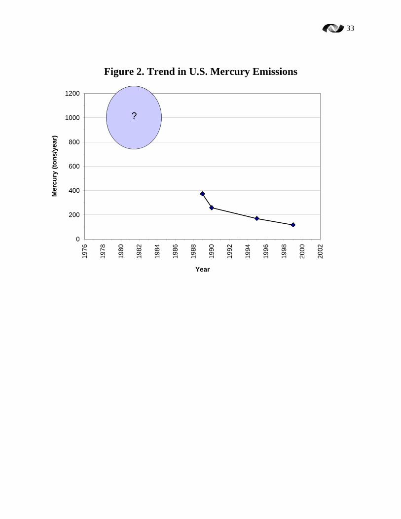
33

Figure 2. Trend in U.S. Mercury Emissions

0

200

400

600

800

1000

120019

76

1978

1980

1982

1984

1986

1988

1990

1992

1994

1996

1998

2000

2002

Year

Mer

cury

(ton

s/ye

ar)

?

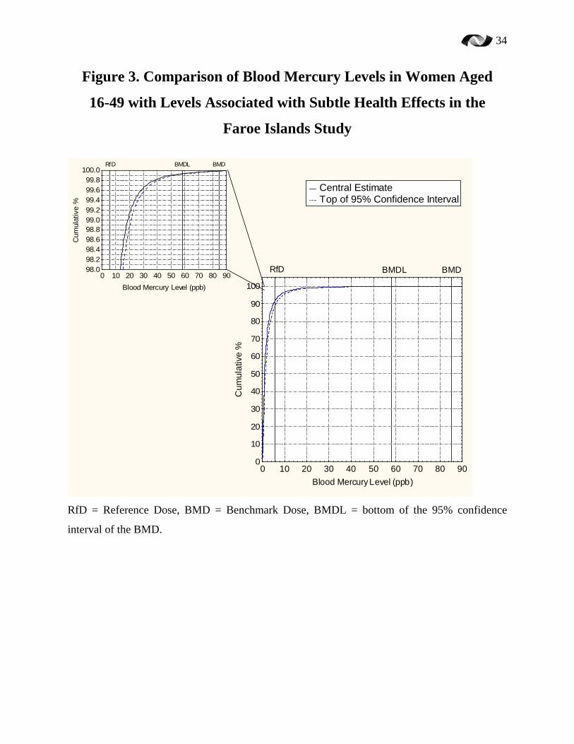
34

Figure 3. Comparison of Blood Mercury Levels in Women Aged

16-49 with Levels Associated with Subtle Health Effects in the

Faroe Islands Study

0 10 20 30 40 50 60 70 80 90Blood Mercury Level (ppb)

0

10

20

30

40

50

60

70

80

90

100

Cum

ulat

ive

%

BMDL BMDRfD0 10 20 30 40 50 60 70 80 90

Blood Mercury Level (ppb)

98.098.298.498.698.899.099.299.499.699.8

100.0

Cum

ulat

ive

%

BMDL BMDRfD

Central Estimate Top of 95% Confidence Interval

RfD = Reference Dose, BMD = Benchmark Dose, BMDL = bottom of the 95% confidence

interval of the BMD.

35

Figure 4. Percent of Women with

Blood Mercury Greater than Given Levels

0%

10%

20%

30%

40%

50%

60%

70%

0.1*RfD 0.5*RfD RfD 2*RfD 3*RfD 5*RfD(0.5*BMDL)

10*RfD(BMDL)

0%

1%

2%

3%

4%

5%

6%

7%

8%

9%

10%

RfD 2*RfD 3*RfD 5*RfD(0.5*BMDL)

10*RfD(BMDL)