radar-aware transmission and scheduling for cognitive
TRANSCRIPT

Rochester Institute of Technology Rochester Institute of Technology
RIT Scholar Works RIT Scholar Works
Theses
5-2020
Radar-Aware Transmission and Scheduling for Cognitive Radio Radar-Aware Transmission and Scheduling for Cognitive Radio
Dynamic Spectrum Access in the CBRS Radio Band Dynamic Spectrum Access in the CBRS Radio Band
Dennis P. Bleier [email protected]
Follow this and additional works at: https://scholarworks.rit.edu/theses
Recommended Citation Recommended Citation Bleier, Dennis P., "Radar-Aware Transmission and Scheduling for Cognitive Radio Dynamic Spectrum Access in the CBRS Radio Band" (2020). Thesis. Rochester Institute of Technology. Accessed from
This Thesis is brought to you for free and open access by RIT Scholar Works. It has been accepted for inclusion in Theses by an authorized administrator of RIT Scholar Works. For more information, please contact [email protected].

Radar-Aware Transmission and Scheduling forCognitive Radio Dynamic Spectrum Access in the
CBRS Radio Band
Dennis P. Bleier

Radar-Aware Transmission and Scheduling forCognitive Radio Dynamic Spectrum Access in the
CBRS Radio BandDennis P. Bleier
May 2020
A Thesis Submittedin Partial Fulfillment
of the Requirements for the Degree ofMaster of Science
inComputer Engineering
COE_hor_k https://www.rit.edu/engineering/DrupalFiles/images/site-lockup.svg
1 of 1 1/9/2020, 10:42 AM
Department of Computer Engineering

Radar-Aware Transmission and Scheduling forCognitive Radio Dynamic Spectrum Access in the
CBRS Radio BandDennis P. Bleier
Committee Approval:
Dr. Andres Kwasinski Advisor DateDepartment of Computer Engineering
Dr. Andreas Savakis DateDepartment of Computer Engineering
Dr. Alexander Loui DateDepartment of Computer Engineering
i

Acknowledgments
I would like to thank my advisor, Dr. Andres Kwasinski, for his support and guid-
ance throughout the project;Dr. Alexander Loui and Dr. Andreas Savakis for being
members of the committee; and the Department of Computer Engineering for letting
me take part in this research.
ii

I would like to dedicate this work to my family and friends. Without your support I
would not have been able to complete this work.
iii

Abstract
Use of the wireless spectrum is increasing. In order to meet the throughput require-
ments, Dynamic Spectrum Access is a popular technique to maximize spectrum usage.
This can be applied to the Citizen Broadband Radio Service (3550-3700MHz), a band
recently opened by the Federal Communications Commission for opportunistic access.
This radio band can be accessed as long as no higher priority users are interfered with.
The top priority users are called incumbents, which are commonly naval radar. Naval
radars transmit a focused beam that can be modelled as a periodic function. Lower
tier users are prohibited from transmitting when their transmissions coincide and
interfere with the radar beam. The second and third tier users are called Priority
Access Licensees and General Authorized Access, respectively. Lower tier users must
account for the transmission outage due to the presence of the radar in their schedul-
ing algorithms. In addition, the scheduling algorithms should take Quality of Service
constraints, more specifically delay constraints into account. The contribution of this
thesis is the design of a scheduling algorithm for CBRS opportunistic access in the
presence of radar that provides Quality of Service for users, consider different traffic
needs.
This was implemented using the ns-3 discrete-event network simulator to simulate
an environment with a radar and randomly placed radios using LTE-U to opportunis-
tically transmit data. The proposed algorithm was compared against the Proportional
Fair algorithm and a Proportional Fair algorithm with delay awareness. Performance
was measured with and without fading models present. The proposed algorithm bet-
ter balanced Quality of Service requirements and minimized the effect of transmission
outage due to presence of the radar.
iv

Contents
Signature Sheet i
Acknowledgments ii
Dedication iii
Abstract iv
Table of Contents v
List of Figures vii
List of Tables viii
Acronyms ix
1 Introduction 1
1.1 Introduction . . . . . . . . . . . . . . . . . . . . . . . . . . . . . . . . 1
1.2 Background . . . . . . . . . . . . . . . . . . . . . . . . . . . . . . . . 2
1.3 Previous Work . . . . . . . . . . . . . . . . . . . . . . . . . . . . . . 7
1.4 Motivation . . . . . . . . . . . . . . . . . . . . . . . . . . . . . . . . . 10
1.5 Novel Contribution . . . . . . . . . . . . . . . . . . . . . . . . . . . . 10
2 System Setup 11
2.1 Physical Layout . . . . . . . . . . . . . . . . . . . . . . . . . . . . . . 11
2.2 Channel Characteristics . . . . . . . . . . . . . . . . . . . . . . . . . 12
2.3 LTE and Internet Protocol . . . . . . . . . . . . . . . . . . . . . . . . 13
2.4 Radar Modelling . . . . . . . . . . . . . . . . . . . . . . . . . . . . . 14
3 Radar-Aware Transmission and Scheduling 16
3.1 Radar-Aware Transmission and Scheduling . . . . . . . . . . . . . . . 16
4 Results 19
4.1 Experimental Setup . . . . . . . . . . . . . . . . . . . . . . . . . . . . 19
4.1.1 NS-3 Setup . . . . . . . . . . . . . . . . . . . . . . . . . . . . 19
4.1.2 Design of Experiments . . . . . . . . . . . . . . . . . . . . . . 20
v

CONTENTS
4.2 No Fading Results . . . . . . . . . . . . . . . . . . . . . . . . . . . . 21
4.2.1 The Process to Final Values . . . . . . . . . . . . . . . . . . . 27
4.3 Fading Results . . . . . . . . . . . . . . . . . . . . . . . . . . . . . . 29
4.4 Overall Result . . . . . . . . . . . . . . . . . . . . . . . . . . . . . . . 32
4.5 Assumptions . . . . . . . . . . . . . . . . . . . . . . . . . . . . . . . . 33
5 Conclusions and Future Work 34
5.1 Conclusion . . . . . . . . . . . . . . . . . . . . . . . . . . . . . . . . . 34
5.2 Future Work . . . . . . . . . . . . . . . . . . . . . . . . . . . . . . . . 34
Bibliography 36
vi

List of Figures
1.1 NS-3 LTE Radio Protocol Stack for eNodeB . . . . . . . . . . . . . . 4
1.2 Reprinted from 3GPP TS 36.213 [1] . . . . . . . . . . . . . . . . . . . 5
1.3 Radar Beam Pattern at 60 RPM . . . . . . . . . . . . . . . . . . . . 8
2.1 User Equipment and EnodeB Layout . . . . . . . . . . . . . . . . . . 12
2.2 Network Topology of Simulated Network . . . . . . . . . . . . . . . . 13
2.3 Radar Beam Observed at Different Locations . . . . . . . . . . . . . . 15
4.1 LTE-EPC Stack in NS-3 [2] . . . . . . . . . . . . . . . . . . . . . . . 20
4.2 Histograms of Proportional Fair No Fading . . . . . . . . . . . . . . . 24
4.3 Histograms of Proportional Fair Delay Aware No Fading . . . . . . . 25
4.4 Histograms of Proposed Algorithm No Fading Traffic . . . . . . . . . 26
4.5 Histogram of Proportional Fair Fading . . . . . . . . . . . . . . . . . 31
vii
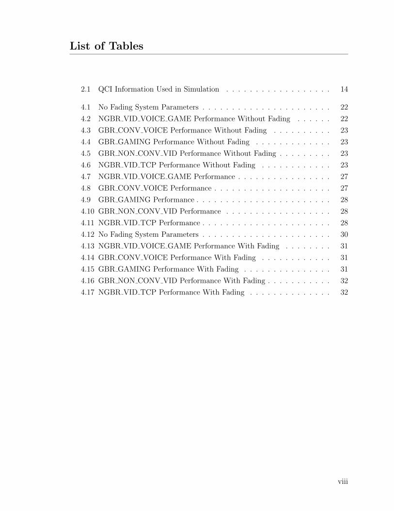
List of Tables
2.1 QCI Information Used in Simulation . . . . . . . . . . . . . . . . . . 14
4.1 No Fading System Parameters . . . . . . . . . . . . . . . . . . . . . . 22
4.2 NGBR VID VOICE GAME Performance Without Fading . . . . . . 22
4.3 GBR CONV VOICE Performance Without Fading . . . . . . . . . . 23
4.4 GBR GAMING Performance Without Fading . . . . . . . . . . . . . 23
4.5 GBR NON CONV VID Performance Without Fading . . . . . . . . . 23
4.6 NGBR VID TCP Performance Without Fading . . . . . . . . . . . . 23
4.7 NGBR VID VOICE GAME Performance . . . . . . . . . . . . . . . . 27
4.8 GBR CONV VOICE Performance . . . . . . . . . . . . . . . . . . . . 27
4.9 GBR GAMING Performance . . . . . . . . . . . . . . . . . . . . . . . 28
4.10 GBR NON CONV VID Performance . . . . . . . . . . . . . . . . . . 28
4.11 NGBR VID TCP Performance . . . . . . . . . . . . . . . . . . . . . . 28
4.12 No Fading System Parameters . . . . . . . . . . . . . . . . . . . . . . 30
4.13 NGBR VID VOICE GAME Performance With Fading . . . . . . . . 31
4.14 GBR CONV VOICE Performance With Fading . . . . . . . . . . . . 31
4.15 GBR GAMING Performance With Fading . . . . . . . . . . . . . . . 31
4.16 GBR NON CONV VID Performance With Fading . . . . . . . . . . . 32
4.17 NGBR VID TCP Performance With Fading . . . . . . . . . . . . . . 32
viii

Acronyms
3GPP
3rd Generation Partnership Project
AMC
Adaptive Modulation and Coding
CBRS
Citizens Broadband Radio Service
CQI
Channel Quality Indicator
CTS
Clear to Send
DSA
Dynamic Spectrum Access
eNB
eNodeB
EPC
Evolved Packet Core
FCC
Federal Communications Commission
ix

Acronyms
GAA
General Authorized Access
GBR
Guaranteed Bit Rate
HOL
Head-of-Line
IP
Internet Protocol
ITU-R
International Telecommunication Union Radiocommunication Sector
LTE
Long Term Extension
LTE-U
Long Term Extension - Unlicensed
MAC
Medium Access Control
MCS
Modulation and Coding Scheme
NGBR
Non-Guaranteed Bit Rate
x

Acronyms
ODFM
Orthogonal Frequency-Division Multiplexing
PAL
Priority Access Licensee
PGW
Packet Data Network Gateway
QAM
Quadrature Amplitude Modulation
QoS
Quality of Service
QPSK
Quadrature Phase Shift Keying
RB
Resource Block
RBG
Resource Block Group
RCQI
Relative Channel Quality Index
RTS
Request to Send
xi

Acronyms
SGW
Serving Gateway
TTI
Transmission Time Interval
UDP
User Datagram Protocol
UE
User Equipment
U.S.
United States
xii

Chapter 1
Introduction
1.1 Introduction
The number of users of wireless radio technologies has greatly increased in the past
few years. This has led to an evolving use of the radio spectrum. Currently, all
radio bands are allocated by the FCC for specific purposes. This leads to high usage
of some spectrum bands and low usage of others. Studies found that up to 82.6%
of the spectrum was unused [3]. Most of this spectrum is inaccessible to common
users, however it does present the idea that commonly used frequency bands may
being inefficiently used. One strategy to use the spectrum more effectively is sharing
through Dynamic Spectrum Access (DSA). This is a technique used in the cognitive
radio paradigm [4] in which a secondary network is established in the same physical
area and frequency band as the primary network. The secondary users will sense the
spectrum for holes, then either transmit on open frequencies in open time periods or
transmit at a power that will not interfere with other users. These techniques are
called interweave and underlay, respectively. In addition to DSA techniques to more
efficiently use the spectrum, the regulatory body controlling spectrum allocation in
the U.S. has noticed the increased need for bandwidth and has opened the CBRS
band of frequencies (3550-3700MHz) to general users. The general users must respect
the previous users of the band, called incumbents, and users that purchase licenses,
1

CHAPTER 1. INTRODUCTION
PAL. The primary incumbent users of the CBRS band are naval radars and satellites.
In addition to the increasing number of people using wireless devices, it should be
noted that a 40% of the population lives on the coast in the United States, even though
this area only accounts for less than 10% of the nations land mass [5]. This means
that many people fall within the exclusion zone that is recommended by regulatory
bodies to protect the functionality of the radar [6]. This provides an opportunity for
spectrum access if the exclusion distance can be reduced or circumvented through
DSA. The close proximity to the coast is notable because it is where naval radars are
usually located.
The unused spectrum and the majority of the population being located close to
the coast is motivation to closely study dynamic spectrum access near the coast. This
may include avoiding naval radar. Naval radar can be modelled as a periodic signal
with a peak in signal every rotation [7].
The contribution of this paper is to present a radar aware scheduling algorithm.
1.2 Background
Over the past few years, usage of the radio spectrum has become an increasingly
important concern. More users than ever are using wireless technologies in their ev-
eryday lives including cellular phones, Bluetooth devices and smart home devices.
This is putting a strain on the limited radio bandwidth that consumers can use.
Those in charge of spectrum allocation have noticed and have started adapting how
the spectrum is used and who can use it. Some bands that are opening will allow
general access, but only if the new devices do not interfere with the incumbent users
of the frequency. One such band is the CBRS band [8]. This consists of frequencies
from 3550 MHz to 3700 MHz, which is unique in pioneering a model for spectrum
sharing. In this band there are three tiers of users, incumbents, which includes the
U.S. Navy, Priority Access Licensees (PAL) and General Authorized Access (GAA)
2

CHAPTER 1. INTRODUCTION
users. The incumbents must not be interfered with. PAL users must not be inter-
fered with by GAA users. GAA users must not interfere with anyone. The primary
incumbent user of the CBRS band is the U.S. Military for radars, satellite providers
and communication. The U.S. population is most dense in port cities near the coast,
which is primarily where radar technologies are used. Some studies have been done
attempting opportunistic transmission in the presence of radar.
The NS-3 discrete network simulator was used to simulate the network environ-
ment. This provides models of packet switched networks. In NS-3, all devices are
nodes. Protocol stacks and applications are then applied to nodes. Applications are
tasks that each nodes completes. The simulator connects devices over an abstract
channel. The channel can be a physical link or a wireless channel. A wireless channel
is used in our simulations. NS-3 has an LTE module that uses the LTE-Evolved
Packet Core (EPC) implementation. The module has been partially designed to sup-
port the evaluation of DSA. The modelling can take many factors into account such
as fading and propagation.
The LTE module is able to track the allocation of individual RBs. This allows
careful tracking to confirm that no eNB will transmit when it is under the radar
beam. In addition, the simulator is able to handle many eNB and even more UE.
This allows a realistic simulation with many different devices. The LTE module has
abstracted each of the layers used in the LTE protocol stack. A diagram of the LTE
stack for the eNB is shown in Figure 1.1.
3

CHAPTER 1. INTRODUCTION
Figure 1.1: NS-3 LTE Radio Protocol Stack for eNodeB
The abstraction of each layer allows scheduling algorithms to be quickly switched
and tested. Traffic that flows from S1-U Devices is able to be kept the same between
experiments. In addition, lower layers such as the physical layers also remain the
same. This system allows for just the performance of the scheduling algorithm to be
tested.
The NS-3 module is able to model Adaptive Modulation and Coding (AMC). This
4

CHAPTER 1. INTRODUCTION
is a process that adjusts the modulation scheme based on channel quality. Period-
ically, the eNodeB (eNB), a LTE base station, sends a reference signal to the User
Equipment (UE), LTE users. Based on the spectral efficiency observed by the User
Equip, a Channel Quality Indicator (CQI) is reported. The CQI is standardized by
the 3GPP in [1]. The table that the UE uses to determine CQI is shown in Figure
1.2.
Figure 1.2: Reprinted from 3GPP TS 36.213 [1]
The higher the efficiency and CQI Index, the higher code rate achievable. There
are three modulation schemes supported by NS-3, Quadrature Phase Shift Keying
(QPSK), 16-quadrature amplitude modulation (16-QAM), and 64-QAM. Modulation
schemes such as 64-QAM support a higher data rates, but are more vulnerable to
interference. The CQI and spectrum efficiency are then used to calculate the MCS.
MCS is an estimation and not exact. There are 28 MCS classes which are used to
calculate which modulation scheme will be used and the size of the transport block.
The transport block is how much data can be effectively transmitted in each resource
block (RB). The RB is a 1ms/180kHz block of time and frequency [9]. This is the
most basic unit in orthogonal frequency-division multiplexing (ODFM) system used
in LTE.
Scheduling is another factor that must be taken into account. Recently, many
5

CHAPTER 1. INTRODUCTION
studies have been performed that optimize how each RB is used. This approach is
possible to apply to the CBRS band even though most current implementations of
LTE use a lesser frequency, some companies are using LTE-U in this band [10].
The first scheduling algorithm that will be leveraged is the proportional fair algo-
rithm as explained by [11]. This algorithm schedules a user when the current channel
quality is high compared to its past quality. In order to calculate this, the algorithm
uses the current achievable rate divided by the past averaged throughput to calculate
a relative channel quality indicator (RCQI). In the NS-3 simulator LTE module [2]
the proportional fair algorithm works as follows. Let i, j be generic users; t be the
subframe index; k be the resource block index; Mi,k(t) be the MCS of user i at RB
k and S(M,B) be the transport block size when B blocks are used. The achievable
rate is calculated by Equation 1.1.
Ri(k, t) =S(Mi,k(t), 1)
τ(1.1)
This calculates the achievable rate for one user, i, using RB k in subframe t. τ is
the duration of one TTI, which is 1ms in LTE. After the achievable rate is calculated,
it is used in Equation 1.2 to allocate each RBG.
ik(t) = argmaxj=1,...,N
(Rj(k, t)
Tj(t)) (1.2)
Tj(t) is the past throughput for user j. This establishes the RCQI as indicated
earlier. The UE with the best RCQI is allocated the RBG. The past throughput for
user j is shown in Equation 1.3.
Tj(t) = (1 − 1
α) ∗ Tj(t− 1) +
1
α∗ Tj(t) (1.3)
The past average throughput is calculated using the exponential moving average
approach. Tj(t) is the throughput achieved by the user j in the subframe t. The
6

CHAPTER 1. INTRODUCTION
process to calculate ˆTj(t) is as follows. First the MCS is determined using Equation
1.4.
Mj(t) = mink:ik(t)=j
Mj,k(t) (1.4)
The minimum supported MCS is used. This gives the best throughput to error
rate. The total number of RBGs allocated to the user is then counted based on the
number of RBGs and when user j had the highest RCQI. The throughput for the
subframe, Tj(t) is then calculated using Equation 1.5.
Tj(t) =S(Mj(t), Bj(t))
τ(1.5)
This is the process for the proportional fair algorithm. This algorithm was fully
implemented within the NS-3 simulator [2]. A delay aware proportional fair algorithm
was created that changed the ik(t) to the equation shown in Equation 1.6.
ik(t) = argmaxj=1,...,N
(exp[wi,j(t) − Tj
Tj+Rj(k, t)
Tj(t)]) (1.6)
This added a delay aware aspect to the proportionally fair algorithm. The usual
proportionally fair algorithm does not have any QoS delay awareness.
The rest of this paper is organized as follows. Chapter II describes the system
setup. The radar aware scheduling algorithm is outlined in Chapter III. Simulation
results are presented in Chapter IV, followed by conclusions in Chapter V.
1.3 Previous Work
Many recent works have focused on DSA in the CBRS band. The most notable to
this thesis is [12]. This studies the feasibility of coexistence of LTE-U with a rotating
radar in the CBRS band. The authors found that it is possible for an LTE-U eNodeB
7
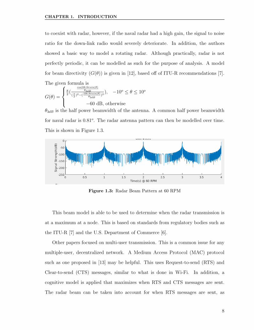
CHAPTER 1. INTRODUCTION
to coexist with radar, however, if the naval radar had a high gain, the signal to noise
ratio for the down-link radio would severely deteriorate. In addition, the authors
showed a basic way to model a rotating radar. Although practically, radar is not
perfectly periodic, it can be modelled as such for the purpose of analysis. A model
for beam directivity (G(θ)) is given in [12], based off of ITU-R recommendations [7].
The given formula is
G(θ) =
π2(
cos(68.8πsin(θ)θ3dB
(π2
)2−((68.8πsin(θ)
θ3dB)2
), −10o ≤ θ ≤ 10o
−60 dB, otherwise
θ3dB is the half power beamwidth of the antenna. A common half power beamwidth
for naval radar is 0.81o. The radar antenna pattern can then be modelled over time.
This is shown in Figure 1.3.
Figure 1.3: Radar Beam Pattern at 60 RPM
This beam model is able to be used to determine when the radar transmission is
at a maximum at a node. This is based on standards from regulatory bodies such as
the ITU-R [7] and the U.S. Department of Commerce [6].
Other papers focused on multi-user transmission. This is a common issue for any
multiple-user, decentralized network. A Medium Access Protocol (MAC) protocol
such as one proposed in [13] may be helpful. This uses Request-to-send (RTS) and
Clear-to-send (CTS) messages, similar to what is done in Wi-Fi. In addition, a
cognitive model is applied that maximizes when RTS and CTS messages are sent.
The radar beam can be taken into account for when RTS messages are sent, as
8

CHAPTER 1. INTRODUCTION
knowledge of the periodic signal will be known and the round trip time for sending
RTS and receiving the CTS message will also be known.
Another paper [14], studied adaptive scheduling. This algorithm places a priority
on each type of traffic based on desired quality-of-service (QoS). There are three
important pieces of the priority function, the k term, which prioritizes real time
traffic when the number of available RBs shrinks, the α term takes into account
the guaranteed delay against the current observed delay and the β term takes into
account the current throughput against the expected throughput. The equation for
the priority function is shown in Equation 1.7.
p(i, j) = kj ∗ exp[αj ∗wi,j(t) − Tj
Tj+ βj ∗
rj − ri,jrj
] (1.7)
p(i, j) is the priority of queue j of user i. i is a generic user. j is a generic traffic
stream. αj and βj are weights to balance delay vs throughput priority. Their sum
should be 1. Tj is the maximum packet delay. rj is the expected packet throughput.
wi,j(t) is the current observed delay of the Head-of-line (HOL) packet. ri,j is the
average througput of traffic queue j of user i. kj is the real time adaptive coefficient.
kj is calculated using Equation 1.8.
kj =
1 + u(N−N)N
, Traffic class j is real-time
1, Traffic class j is non-real-time(1.8)
N is the mean number of available subchannels and N is the number of sub-
channels currently available. u() is the unit-step function. Using kj places a higher
priority on real-time traffic when available channels decrease. This will be helpful
in providing a QoS based scheduling algorithm. Many of the other algorithms only
take the channel quality into effect or are not adaptive. In addition, many scheduling
algorithms are not aware of QoS requirements.
9

CHAPTER 1. INTRODUCTION
1.4 Motivation
The motivation for this work is to more efficiently use the radio spectrum in the
coastal areas. This is an area with a high population density and will require a more
optimally used spectrum to service an increasing number of user’s data needs. End
users will be able to take advantage of the higher throughput to support applications
such as video streaming and browsing social media.
1.5 Novel Contribution
The new idea present is a periodically changing scheduler. Based on the rotation of
the radar, the availability of the transmitter and routes will change. The scheduling
algorithm will detect when the radar beam is overhead and know when the transmitter
is able to transmit. It is assumed that the radar is perfectly periodic.
The scheduling algorithm does not just mute transmission, it uses the amount
of time transmission will be muted due to the radar, the current channel conditions
and QoS requirements in order to maintain the required QoS most efficiently. This
allows users to experience the QoS that is expected and does not interfere with the
incumbent radar. By using real-time channel quality measurements, the base station
can maximize overall throughput in addition to maintaining QoS requirements.
10

Chapter 2
System Setup
Using the NS-3 simulator, a simulation environment was created. This simulator
allows the entire LTE stack and Internet Protocol (IP) to be simulated and takes a
variety of factors into account including physical layout, fading, and Adaptive Modu-
lation and Coding (AMC). In the simulated system, there were five UE and one eNB.
This was used for all of the simulations. Simulations were run until the queue length
reached a steady state.
2.1 Physical Layout
For the simulations, an eNB was placed, then five UE placed in a uniform disc around
the eNB. The distance between could be adjusted to vary the effects of fading and
propagation loss on the signal. Figure 2.1 shows the physical layout of the setup.
11

CHAPTER 2. SYSTEM SETUP
Figure 2.1: User Equipment and EnodeB Layout
This layout keeps the propagation loss the same for all of the UE. Signal degra-
dation due to fading will be different. While each UE experiences different fading,
it is constant between each run, so that the channel conditions are consistent when
different scheduling algorithms are tested.
2.2 Channel Characteristics
Signal degradation was simulated. Propagation loss and fading were able to be sim-
ulated. Some experiments were run without fading. The Friis Model was used as
12

CHAPTER 2. SYSTEM SETUP
outlined in [15] for both path loss and fading. Simulating these increases how realis-
tic the channel is modelled.
In addition, the adaptive modulation and coding system that was mentioned in
Section 1.2 was used. This changes the size of the transport block based on the
channel condition from fading and propagation loss. This is a realistic system that is
used that varies the throughput that a channel can experience.
2.3 LTE and Internet Protocol
In the simulation, the IP stack was installed on the eNB and UE. In order to sim-
ulate traffic, an external device connected through the internet sent User Datagram
Protocol (UDP) traffic to each UE. The network topology is shown in Figure 2.2.
Figure 2.2: Network Topology of Simulated Network
The Packet Data Network Gateway (PGW) and Serving Gateway (SGW) are
nodes that are part of the Evolved Packet Core (EPC). This is part of the LTE
model. The PGW provides access to the internet and other services to down-link
users. The SGW receives and forwards packets from the PGW to the correct eNB.
The SGW also keeps track of IP bearer services. The Evolved Packet System (EPS)
as outlined in [16] is maintains QoS for the UE.
The EPS bearer uses QoS Class Identifiers (QCI) to ensure traffic QoS require-
ments are upheld. This signals to the eNB what type of traffic is being transmitted.
This is used to keep traffic under delay constraints and under packet error loss rates.
13

CHAPTER 2. SYSTEM SETUP
There were five different traffic classes used in simulation. These are shown with their
QCI identifier, resource type, delay budget and example services in Table 2.1.
QCI Resource Type Max Delay Example Services
1 GBR 100ms Conversational Voice
3 GBR 50ms Real Time Gaming
4 GBR 300ms Non-Conversational Video
7 Non-GBR 100ms Video (Live Streaming), Interactive Gaming
9 Non-GBR 300ms TCP-Based Buffered Video Streaming
Table 2.1: QCI Information Used in Simulation
The resource type is if the traffic has a guaranteed bit rate or not. Guaranteed bit
rate traffic has a bandwidth that is guaranteed. There are many other QCI indicators
outlined in [16], but only five were used in the simulation.
2.4 Radar Modelling
In the simulations, a simple model was used for the radar. The model from the ITU-
R [7] and shown in [12] was used. The pattern is shown in 1.3. An experiment was
conducted using Matlab. Using the previously mentioned model, observation of the
radar was done at different points. The observed peak of the radar is different based
on location. Examples of this are shown in Figure 2.3.
14

CHAPTER 2. SYSTEM SETUP
Figure 2.3: Radar Beam Observed at Different Locations
The observed peak is shifted at each location. This is a very simple model of
the radar, but is sufficient. Four distinct locations were shown, but there are many
more possible. An interactive program was created in Matlab that allowed the user
to move a point around a circle and the observed radar beam would be shown.
15

Chapter 3
Radar-Aware Transmission and Scheduling
3.1 Radar-Aware Transmission and Scheduling
The scheduling algorithm is different from classic schedulers in that it is able to dy-
namically change based on channel conditions and in our case based on the radar.
The proposed algorithm uses the current HOL delay of the queues and the current
channel conditions to provide timely transmission of packets. In addition, the pro-
posed algorithm puts a priority on GBR traffic, to minimize the radar effects on
guaranteed traffic. The algorithm is also aware of when each UE will experience the
effect of the radar and boosts transmission such that the overall delay experienced
will be minimized.
In order to create this algorithm, the proportional fair algorithm was studied.
This provided a good starting point that balanced all of the traffic. Packets are
scheduled based on their relative channel quality and past throughput. When there
are no differentiating factors between UE, all of the traffics will have the same average
throughput. Next, a boost period was added. This is for all traffic classes and provides
a temporary boost to each stream by adding the upcoming delay onto the traffic queue
length. This prioritizes the traffic that is about to be muted due to the radar beam.
Next, a delay aware aspect was added to the algorithm. This was adapted from the
adaptive scheduling algorithm in [14]. The priority equation shown in Equation 1.7
16

CHAPTER 3. RADAR-AWARE TRANSMISSION AND SCHEDULING
was changed and merged with the proportional fair algorithm. The α term focuses
on the delay and the β term is the proportional fair aspect. The sum of the α and β
terms is one. The terms can be changed to place a higher weight on the delay aspect
or the proportional fair aspect of scheduling. Another part of [14] that was adapted
was the k term becoming the p term. In the previous adaptive algorithm, the k term
added a higher priority to real-time traffic when the amount of available subchannels
dropped below the mean available amount of subchannels. In the proposed situation,
the number of available subchannels is more consistent, but when the radios can
transmit is changing. The adaptation has been made to change the k, which is in
the frequency domain, to the p term, which is the time domain. The p term becomes
active when there is less than the mean time remaining until the radar beam causes
the radio to mute. This allows GBR traffic to more likely meet QoS requirements.
All of the equations used in the calculation are shown below.
First, the achievable rate is calculated the same as the proportional fair algorithm
as shown in Equation 1.1. Let i be a generic user and j be a flow of user i The
algorithm then allocates RBGs to active users using Equation 3.1.
ik = argmaxj=1,...,N
0, tj,off < t < tj,on
pj ∗ exp[αj ∗ wi,j(t)−TjTj
+ βj ∗ Rj(k,t)
Tj(t)] , otherwise
(3.1)
tj,off is the time when flow j must be muted as to not interfere with the radar.
tj,on is when the flow j is able to resume transmission. αj and βj are weights that
change how much weight is placed on the delay awareness or the channel awareness.
Their sum is 1. Tj is the maximum allowed delay as required from QCI. Rj(k, t) is the
achievable rate for the stream j in the current RB. Tj(t) is the exponential moving
average throughput of the stream j as calculated in Equation 1.3. pj is the priority of
the stream j. wi,j(t) is the queue delay experienced by stream j for user i, in addition
to a boost in performance when the radar is approaching. This is calculated using
17

CHAPTER 3. RADAR-AWARE TRANSMISSION AND SCHEDULING
Equation 3.2.
wi,j(t) =Qi,j(t)
Rj(k, t)+ u(t− tj,off + ∆tj) ∗ 1.5∆tj (3.2)
In this equation, Qi,j(t) is the length of the queue of stream j. u(·) is the unit-step
function. ∆tj is the amount of time that the radio is muted to not interfere with the
radar. By accounting for the delay due to the radar, peaks in queue delay are able to
be minimized. Another part that helps minimize queue delay for GBR traffic is the
priority term pj. The equation for this is shown in Equation 3.3.
pj =
1 +u(tavg−tremaining)
tavg∗2, GBR Traffic
1, Non-GBR Traffic(3.3)
In this equation, tavg is the average time remaining before the transmitter is
required to mute and tremaining is the amount of time remaining before the transmitter
is required to mute. As the time approaches that the radio must mute transmissions,
the pj term increases, putting a higher priority on GBR traffic. After the RBGs are
allocated, the remaining steps in the proportional fair algorithm are followed including
calculating the proper MCS as shown in Equation 1.4 and the actual throughput for
the user i in subframe at t as shown in 1.5.
The algorithm prioritizes GBR traffic, minimizes the effect of muting for the radar
of packet delay and maintains delay requirements according to QCI.
18

Chapter 4
Results
There were two main simulation scenarios that were run, with fading and without
fading. Three algorithms are compared, the proportional fair, as outlined in [11] and
Section 1.2, proportional fair with delay awareness, as outlined in Section 1.2 and
the proposed algorithm, as outlined in Chapter 3.1. For each of these the αj and
βj terms were adjusted. The αj term determines how much weight is placed on the
queue delay and the βj term weights how much the scheduler will perform like the
proportional fair.
4.1 Experimental Setup
4.1.1 NS-3 Setup
The simulator used was the NS-3 simulator. This simulates all of the discrete events
within Internet Systems [2]. This is organized in such a way that user modules can
be created and all source code is available to edit. Each part of the network is broken
into modules and most have classes that assist the user with setup and customization.
In addition, there are plenty of examples to help new users get started. The NS-3
simulator allows simulation of the LTE-EPC stack and allows for IP connectivity with
only a few lines of code for setup. The IP stack can be used between two devices easily
without the user having to worry about implementing their functionality. Figure 4.1
19

CHAPTER 4. RESULTS
shows how this is implemented.
Figure 4.1: LTE-EPC Stack in NS-3 [2]
Each of the blocks are different parts of the LTE-EPC stack and can be modi-
fied. For the experiment, the MAC layer of the eNB was modified to implement the
proposed algorithm and the other algorithms that were used for comparison. A new
module was added to MAC layer. The downlink scheduling function was modified
to determine the results. In NS-3 this function is called DoSchedDlTriggerReq. The
changes that were made to implement the proposed algorithm were assigning each
stream an offset of when they would be required to turn off, adding awareness of
turning off to the scheduling function and implementing the proposed algorithm to
select which UE will get allocated each RB.
4.1.2 Design of Experiments
For the experiments, a variety of traffic classes were present. These included both
GBR and NGBR traffic. Also, traffic with different delay constraints were selected.
Traffic was also selected to reflect real use of a network with different services. Classes
that support services such as buffered video streaming, live-streaming video, online
gaming and conversational voice were used. Another change that was made for each of
20

CHAPTER 4. RESULTS
the simulations was the packet size. This was determined by using different values and
increasing until the system reached a steady state without all traffic classes meeting
their QoS requirements all of the time. If the packet size decreased then all traffic
would meet their requirements and the comparison would be more difficult to observe.
If the packet size is decreased too much, then all traffic classes will perform similarly,
as there is not enough traffic to load the network.
In order to determine which αj and βj terms performed the best, simulations were
run that changed each of the weights by 0.05. These were repeated until a good
balance between the GBR and NGBR traffic was reached. The goal is to minimize
the amount of time that the traffic is above the delay constraint. Once a good balance
was reached, the traffic was changed by 0.01 to find the most optimal. There were
multiple ratios that performed favorably.
4.2 No Fading Results
The partial simulation parameters are shown in Table 4.1 below.
21

CHAPTER 4. RESULTS
Parameter Value
Packet Size 2160 Bytes
Packet Arrival Rate 200 / s
Delay Due to Radar 50 ms
GBR αj value 0.4
GBR βj value 0.6
NGBR αj value 0.6
NGBR βj value 0.4
UE Distance from ENb 100m
θ3dB of Radar 0.81o
Radar Rotation Speed 60 rpm
Table 4.1: No Fading System Parameters
The parameters for αj and βj were found by varying the values and finding which
resulted in the best performance. Many experiments were run will small changes to
the αj and βj terms. The results were then recorded against each other and the result
that had the best relative performance between the GBR and NGBR was selected.
The results for the simulation without fading are shown in the Tables below.
NGBR VID VOICE GAME Maximum QoS Delay: 100ms
Mean Delay (ms) Standard Deviation (ms) Maximum Delay (ms) Probability Over
Proposed Algorithm 92.1 15.9 162.0 0.221
Proportional Fair 12.6 11.2 93.7 0
Proportional Fair + Delay Awareness 91.9 21.8 230.4 0.208
Table 4.2: NGBR VID VOICE GAME Performance Without Fading
22

CHAPTER 4. RESULTS
GBR CONV VOICE Maximum QoS Delay: 100ms
Mean Delay (ms) Standard Deviation (ms) Maximum Delay (ms) Probability Over
Proposed Algorithm 76.9 18.4 116.4 0.045
Proportional Fair 11.9 7.8 54.8 0
Proportional Fair + Delay Awareness 85.6 20.7 143.3 0.153
Table 4.3: GBR CONV VOICE Performance Without Fading
GBR GAMING Maximum QoS Delay: 50ms
Mean Delay (ms) Standard Deviation (ms) Maximum Delay (ms) Probability Over
Proposed Algorithm 34.4 13.4 69.1 0.046
Proportional Fair 12.7 7.6 55.0 0.004
Proportional Fair + Delay Awareness 40.4 16.8 104.5 0.160
Table 4.4: GBR GAMING Performance Without Fading
GBR NON CONV VID Maximum QoS Delay: 300ms
Mean Delay (ms) Standard Deviation (ms) Maximum Delay (ms) Probability Over
Proposed Algorithm 255.9 41.4 384.9 0.159
Proportional Fair 13.5 7.9 54.6 0
Proportional Fair + Delay Awareness 283.6 43.7 516.3 0.260
Table 4.5: GBR NON CONV VID Performance Without Fading
NGBR VID TCP Maximum QoS Delay: 300ms
Mean Delay (ms) Standard Deviation (ms) Maximum Delay (ms) Probability Over
Proposed Algorithm 276.7 31.7 460.3 0.146
Proportional Fair 11.7 7.2 51.9 0
Proportional Fair + Delay Awareness 258.6 41.8 515.2 0.092
Table 4.6: NGBR VID TCP Performance Without Fading
In this case, the proportional fair algorithm was able to outperform the others, as
it was not concerned with the delays and there was enough bandwidth that allowed
all users to stay under their delay constraints. The effects of the p, α and β terms
were able to be seen. These are reflected in a lower Mean Delay (ms) for the gam-
ing traffic in the proposed algorithm, compared to the proportional fair with delay
awareness. The radar-aware aspect of the proposed algorithm was able to minimize
23

CHAPTER 4. RESULTS
the max delay which caused all traffic classes had a lower maximum delay than the
proportional fair + delay awareness. Histograms were also created that showed the
distribution of queue delay throughout the simulation. The histogram for propor-
tional fair simulation is shown in Figure 4.2.
Figure 4.2: Histograms of Proportional Fair No Fading
As expected, all of the traffic has a very similar distribution. Proportional fair
keeps the throughput of the streams equal. This is because all of the channels have
the same channel conditions. There is no difference to how the proportional fair
scheduler treats the GBR and NGBR traffic. Next, the histogram of the proportional
fair with delay awareness is shown in Figure 4.3.
24

CHAPTER 4. RESULTS
Figure 4.3: Histograms of Proportional Fair Delay Aware No Fading
This algorithm had more spread than the proportional fair due to the delay
awareness. The two streams with the highest delay, GBR NON CONV VID and
NGBR VID TCP were separate from the other three. There is similar performance
of the GBR NON CONV VID and NGBR VID TCP because both of their delay
constraints are 300ms. There are also similarities between the GBR CONV VID and
NGBR VID VOICE GAME traffic because they have the same delay constraint of
100ms. THE GBR GAMING traffic has many points that are in the first two classes
of 20ms and 40ms because the delay constraint is 50ms. This is true for the The
histogram of the proposed algorithm is shown in Figure 4.4.
25

CHAPTER 4. RESULTS
Figure 4.4: Histograms of Proposed Algorithm No Fading Traffic
The proposed algorithm has a wider distribution than the other algorithms, due
to the multiple factors that the proposed algorithm takes into account. This allows
better performance for the low latency QoS flows. Within these graphs, the tail to the
left, prominent in the GBR CONV VOICE traffic, is due to the priority that is placed
on GBR traffic and the boost period that is present immediately prior to ceasing
transmissions for the radar. The tail of the right, easily seen in the NGBR VID TCP
traffic, is due to the stopping transmissions to not interfere with the radar. There is
also some differentiation between the GBR and NGBR traffic with the same delay
constraints. This is because the proposed algorithm places a higher priority on the
26

CHAPTER 4. RESULTS
GBR traffic. Due to overall throughput being a finite resource, the NGBR traffic
suffers worse performance.
4.2.1 The Process to Final Values
There were a variety of attempts prior to finding a favorable result. Different values
for αj and βj were used in addition to using different values in the denominator of
the priority function. The tables below shows some of the intermediate steps, along
with a reference.
NGBR VID VOICE GAME Maximum QoS Delay: 100ms
Mean Delay (ms) Standard Deviation (ms) Maximum Delay (ms) Probability Over
Reference 92.2 15.6 164.6 0.222
P Value 1/1 103.3 18.2 184.0 0.642
P Value 1/4 83.2 14.7 151.2 0.085
Both Alpha 0.75 94.8 19.4 166.1 0.364
Both Alpha 0.25 113.8 21.0 224.8 0.805
No Radar Delay 95.5 21.5 246.6 0.239
Table 4.7: NGBR VID VOICE GAME Performance
GBR CONV VOICE Maximum QoS Delay: 100ms
Mean Delay (ms) Standard Deviation (ms) Maximum Delay (ms) Probability Over
Reference 71.3 18.4 108.5 0.016
P Value 1/1 62.6 22.3 108.9 0.030
P Value 1/4 73.6 16.3 122.7 0.022
Both Alpha 0.75 73.6 18.5 121.2 0.028
Both Alpha 0.25 55.1 20.5 95.8 0
No Radar Delay 73.6 18.7 118.9 0.024
Table 4.8: GBR CONV VOICE Performance
27

CHAPTER 4. RESULTS
GBR GAMING Maximum QoS Delay: 50ms
Mean Delay (ms) Standard Deviation (ms) Maximum Delay (ms) Probability Over
Reference 32.1 12.7 65.5 0.030
P Value 1/1 28.7 12.9 55.6 0.058
P Value 1/4 33.0 12.5 73.3 0.037
Both Alpha 0.75 33.0 13.0 66.4 0.034
Both Alpha 0.25 25.4 11.4 51.0 0
No Radar Delay 34.6 14.2 94.1 0.076
Table 4.9: GBR GAMING Performance
GBR NON CONV VID Maximum QoS Delay: 300ms
Mean Delay (ms) Standard Deviation (ms) Maximum Delay (ms) Probability Over
Reference 237.3 41.7 370.0 0.086
P Value 1/1 211.8 42.3 317.5 0.012
P Value 1/4 242.5 39.0 380.9 0.089
Both Alpha 0.75 245.1 42.6 389.0 0.134
Both Alpha 0.25 193.5 35.0 310.1 0.000
No Radar Delay 239.2 43.1 446.3 0.082
Table 4.10: GBR NON CONV VID Performance
NGBR VID TCP Maximum QoS Delay: 300ms
Mean Delay (ms) Standard Deviation (ms) Maximum Delay (ms) Probability Over
Reference 282.0 30.5 468.2 0.153
P Value 1/1 327.8 35.5 529.3 0.818
P Value 1/4 243.7 29.4 408.2 0.037
Both Alpha 0.75 294.0 35.0 487.6 0.348
Both Alpha 0.25 375.7 41.7 611.9 0.996
No Radar Delay 283.8 39.8 571.2 0.156
Table 4.11: NGBR VID TCP Performance
The reference is the proposed algorithm as is. The P value 1/1 places a much
higher priority on the GBR traffic, at the cost of the NGBR traffic. This changes the
denominator of the P function shown in Equation 3.3. This change removed the factor
28

CHAPTER 4. RESULTS
of two. The P value 1/4 changed the factor in the denominator to 4. This placed
too little priority on the GBR traffic, which allowed the NGBR traffic to outperform
it. Changing both of the α values to 0.75 had no meaningful effect on the result
and overall decreased performance. Changing both of the α values to 0.25 allowed
the GBR traffic to thrive, but came at a very steep cost to the NGBR traffic. The
simulation without radar delay did not artificially increase the length of the queue
prior to the transmitter turning off. This led to higher maximum delays and slightly
worse performance for the NGBR traffic.
The tables shown above show that a balance is required. If one term is allowed
to overpower the others, it will cause one type of traffic to gain too much and the
others suffer. The proposed algorithn was able to balance the factors shown above
successfully.
4.3 Fading Results
The experiment was then repeated with fading effecting the channel. This reduces
the quality of the channel. Algorithms such as the proportional fair do not take
into account the queue delay, and thus only maximize the channels that have a good
quality. Because of the degradation in channel quality, the achievable throughput
decreased. The Friis model [15] was used to simulate the effects of fading. This
model is based on the distance the UE are from the eNB The parameters used in the
simulation are shown in Table 4.12.
29

CHAPTER 4. RESULTS
Parameter Value
Packet Size 1140 Bytes
Packet Arrival Rate 200 / s
Delay Due to Radar 50 ms
GBR αj value 0.62
GBR βj value 0.38
NGBR αj value 0.48
NGBR βj value 0.52
UE Distance from ENb 10m
θ3dB of Radar 0.81o
Radar Rotation Speed 60 rpm
Table 4.12: No Fading System Parameters
In addition to the throughput decreasing, the distance between the eNB and UE
was required to decrease. Radio signals degrade logarithmically and at the previously
used distance of 100m, the signal was not strong enough to transmit any data. To
determine the αj and βj weights for this simulation, the simulation was run with 10
of the possible 120 UE combinations and performance was based off of the average.
When a favorable balance was achieved, the simulation was run with all 120 UE
combinations and the results were averaged. A histogram of the performance of the
proportional fair algorithm is shown in Figure 4.5.
30

CHAPTER 4. RESULTS
Figure 4.5: Histogram of Proportional Fair Fading
Because the performance is highly related to channel quality, the algorithm pri-
oritized the good channel. This led to neglect of the other traffic and once a steady
state was reached, the three streams were all much over their maximum constraints.
For this reason, the proportional fair algorithm was excluded from the fading results.
The results from the experiment with fading are shown below.
NGBR VID VOICE GAME Maximum QoS Delay: 100ms
Mean Delay(ms) Standard Deviation(ms) Maximum Delay(ms) Probability Over
Proposed Algorithm 62.8 19.9 127.1 0.155
Proportional Fair + Delay Awareness 38.0 14.5 103.2 0.063
Table 4.13: NGBR VID VOICE GAME Performance With Fading
GBR CONV VOICE Maximum QoS Delay: 100ms
Mean Delay(ms) Standard Deviation(ms) Maximum Delay(ms) Probability Over
Proposed Algorithm 38.9 16.1 90.6 0.029
Proportional Fair + Delay Awareness 40.4 14.8 105.8 0.068
Table 4.14: GBR CONV VOICE Performance With Fading
GBR GAMING Maximum QoS Delay: 50ms
Mean Delay(ms) Standard Deviation(ms) Maximum Delay(ms) Probability Over
Proposed Algorithm 19.0 10.3 59.4 0.023
Proportional Fair + Delay Awareness 16.6 10.2 71.4 0.020
Table 4.15: GBR GAMING Performance With Fading
31

CHAPTER 4. RESULTS
GBR NON CONV VID Maximum QoS Delay: 300ms
Mean Delay(ms) Standard Deviation(ms) Maximum Delay(ms) Probability Over
Proposed Algorithm 141.9 32.13 262.0 0.063
Proportional Fair + Delay Awareness 116.0 21.8 226.5 0.029
Table 4.16: GBR NON CONV VID Performance With Fading
NGBR VID TCP Maximum QoS Delay: 300ms
Mean Delay(ms) Standard Deviation(ms) Maximum Delay(ms) Probability Over
Proposed Algorithm 225.4 38.0 379.7 0.233
Proportional Fair + Delay Awareness 113.3 22.6 220.4 0.029
Table 4.17: NGBR VID TCP Performance With Fading
For this simulation, the channel quality was varied for each user and an average
taken. This allowed all users to experience favorable and unfavorable conditions.
The proposed algorithm places a higher emphasis on the the GBR traffic. This has
a negative effect on the NGBR traffic. The α and β terms allow the balance of the
two. These values changed due to the change in channel characteristics.
4.4 Overall Result
By utilizing the α and β terms, the proposed algorithm was able to effectively balance
the QoS delay restraints of GBR traffic and NGBR traffic. Because there is limited
bandwidth, the improved performance of the GBR traffic came at the cost of the
NGBR traffic. Although there was a decrease in performance, the NGBR traffic was
able to remain under the delay constraint up to 89% of the time. The α and β terms
allowed this as there is a trade off between how closely the algorithm weights the
delay aware aspect and the proportional fair.
32

CHAPTER 4. RESULTS
4.5 Assumptions
In order to obtain the results, some assumptions needed to be made. The first is
that the eNB is able to transmit to each of the UE separately. If this was not true
then each time the eNB stopped transmitting, all of the queues would grow by the
amount of time the eNB was not transmitting for. This increase would not be able to
be reduced without the eNB using more RBs. This would be a serious assumption to
break. The next assumption was that all of the UE were equidistantly placed around
the eNB. If the UE were all placed very close together, their transmissions would be
required to cease at the same time. If this were violated, a situation similar to the
first assumption would be present. As long as there is reasonable spacing between
the UE, this is not as serious. Another assumption is that the radar is perfectly
periodic without side lobes, that should not be interfered with or cause interference.
This would lead to different pattern of eNB transmission stoppage. The model also
assumes that all UE are stationary. If this were violated, when the eNB stopped
transmitting to each UE would constantly change. This could lead to interference
with the radar beam if the eNB transmission did not stop at the proper time.
33

Chapter 5
Conclusions and Future Work
5.1 Conclusion
In conclusion a radar-aware scheduling algorithm was created. NS-3 was used to
simulate a wireless situation in which a radar was simulated. This discrete network
simulator was used to simulate the LTE stack and the IP stack. The proposed al-
gorithm was able to successfully balance the QoS requirements of GBR and NGBR
traffic. Without fading present. the proposed algorithm had minimal degradation in
NGBR quality, with a large increase in quality to the GBR traffic. In the case of
fading, the NGBR traffic performance suffered more, but the increase to GBR traffic
was still present. This algorithm can allow more efficient use of the CBRS band in
the densely populated coastal areas. This allows users to experience higher quality
wireless communications.
5.2 Future Work
Future work could include using a more complex model for the radar. The model
used was simple and actual radar is more complex than the moving average used.
The αj term and βj term could be optimized for each individual QCI. Currently the
algorithm was tested using a variety of values for the αj and βj for the GBR and
NGBR traffic. Other antenna models could be used and explored to show their effect
34

CHAPTER 5. CONCLUSIONS AND FUTURE WORK
on transmissions. Another future exploration could be adding mobility to each of the
UE. This would be more realistic and also require the UE to take the current and
next position of the UE to determine when to stop transmitting, as to not interfere
with the radar beam.
35
Bibliography
[1] 3GPP, “Evolved Universal Terrestrial Radio Access (E-UTRA); Physical layerprocedures ,” 3rd Generation Partnership Project (3GPP), Technical Specifica-tion (TS) 36.213, 10 2014, version 12.3.0. [Online]. Available: https://www.etsi.org/deliver/etsi ts/136200 136299/136213/12.03.00 60/ts 136213v120300p.pdf
[2] ns 3 Project, “Lte module - design documentation.” [Online]. Available:https://www.nsnam.org/docs/models/html/lte-design.html
[3] M. A. McHenry, P. A. Tenhula, D. McCloskey, D. A. Roberson, and C. S. Hood,“Chicago spectrum occupancy measurements & analysis and a long-term studiesproposal,” in TAPAS ’06, 2006.
[4] J. Mitola, G. Q. Maguire et al., “Cognitive radio: making software radios morepersonal,” IEEE personal communications, vol. 6, no. 4, pp. 13–18, 1999.
[5] “2011 to 2015 american community survey.” [Online]. Available: https://www.census.gov/acs/www/data/data-tables-and-tools/data-profiles/2015/
[6] L. E. S. G. Locke and A. Secretary, “An assessment of the near-term viabilityof accommodating wireless broadband systems in the 1675-1710 mhz 1755-1780mhz 3500-3650 mhz and 4200-4220 mhz 4380-4400 mhz bands,” October 2010.
[7] “Mathematical models for radiodetermination radar systems antenna patternsfor use in interference analysis,” Recommendation, ITU-R M.1851, Tech. Rep.,Jun. 2009.
[8] 3GPP, “Citizens Broadband Radio Service (CBRS) 3.5 GHz bandfor LTE in the United States,” 3rd Generation Partnership Project(3GPP), Technical Specification (TS) 36.744, 01 2017, version 14.0.0.[Online]. Available: https://portal.3gpp.org/desktopmodules/Specifications/SpecificationDetails.aspx?specificationId=3103
[9] ——, “Group radio access network; physical channel and modulation (release 8)ts 36.211,” 3GPP, Tech. Rep., 2009.
[10] “Ongo wireless coverage - in-building, public space & industrial iot: Cbrsalliance,” Oct 2019. [Online]. Available: https://www.cbrsalliance.org/
[11] S. Sesia, I. Toufik, and M. Baker, Multi-User Scheduling and InterferenceCoordination. Wiley, 2011, pp. 279–292. [Online]. Available: https://ieeexplore.ieee.org/document/8045774
[12] N. Nurani Krishnan, N. Mandayam, I. Seskar, and S. Kompella, “Experiment:Investigating feasibility of coexistence of lte-u with a rotating radar in cbrsbands,” in 2018 IEEE 5G World Forum (5GWF), 07 2018, pp. 65–70.
36
BIBLIOGRAPHY
[13] Q. Zhao, L. Tong, A. Swami, and Y. Chen, “Decentralized cognitive mac foropportunistic spectrum access in ad hoc networks: A pomdp framework,” Cal-ifornia Univ Davis Dept. of Electrical and Computer Engineering, Tech. Rep.,2007.
[14] J. Li, B. Xu, Z. Xu, S. Li, and Y. Liu, “Adaptive packet scheduling algorithm forcognitive radio system,” in 2006 International Conference on CommunicationTechnology, Nov 2006, pp. 1–5.
[15] H. T. Friis, “A note on a simple transmission formula,” Proceedings of the IRE,vol. 34, no. 5, pp. 254–256, 1946.
[16] 3GPP, “Universal Mobile Telecommunications System (UMTS);LTE; Architec-ture enhancements for non-3GPP accesses,” 3rd Generation Partnership Project(3GPP), Technical Specification (TS) 36.402, 11 2014, version 11.4.0. [Online].Available: https://www.etsi.org/deliver/etsi ts/136200 136299/136213/12.03.00 60/ts 136213v120300p.pdf
37