radial and pruned tetrahedral interpolation techniques · 3 a cube is returned from the color table...

Radial and Pruned Tetrahedral Interpolation Techniques Gary L. Vondran Hewlett-Packard Laboratories - Cambridge HPL-98-95 radial, tetrahedral, pruned tetrahedral, interpolation, color mapping, color space conversion, cube subdivision, image processing, color processing

Presented are two new interpolation approaches based on CubeSubdivision. The first, Radial Interpolation, exploits the observation that the subcube in each iteration can be generated by averaging the vertex of the cube indexed by the slice across the input values with all other vertices of the cube. This leads to further optimizations, resulting in Radial Interpolation requiring only n+1 table accesses and n+1 additions to generate each pixel output component, when interpolating using n bits. The second, Pruned Tetrahedral Interpolation, takes advantage of pruning techniques to implement a tetrahedral interpolation in 2n additions for each pixel output component. Also presented is an implementation that can perform both Radial and Pruned Tetrahedral Interpolations. Finally, Non-Symmetric Radial and Pruned Tetrahedral Interpolation approaches are presented that allow for interpolation with a non-symmetric color table.

External Posting Date : Oct 22, 2009 [Fulltext] Approved for External Publication

Internal Posting Date: April, 1998 [Fulltext]

© Copyright 1998 Hewlett-Packard Development Company, L.P.

2

1. Background

When working with color data, it is a common desire to convert the data from one color space rep-resentation into another. A scanner may use the additive color space RGB (Red, Green, Blue)while printers use the subtractive color space CMY (Cyan, Magenta, Yellow). Other spacesinclude CMYK (Cyan, Magenta, Yellow, and Black), CieLab, YCbCr, LUV, LHS, and others. Toallow these devices to interact, a method is needed to convert the data from the color space of onedevice to the color space of another.

1.1 Color Space Conversion ProcessIdeally a mathematical formula can be used for color space conversion. Some conversions can beperformed with a linear matrix multiply while others have complex non-linear relationships. Inaddition, translations to expand the color gamut and correct for imperfections in the reading, dis-playing, and printing devices are also performed on the color data. It is generally desired to com-bine these translations into the color conversion process in order to reduce computations. It is alsodesired that the implementation be flexible such that it may be used to translate from any colorspace to any other color space, including device corrections.

The most direct approach that satisfies all these wants is a lookup table. The advantages of alookup table are that it is simple and can be used for any translation. The translation performed isdetermined by the table used. The drawback, however, is that these tables can be enormous. Aconversion from a 24 bit RGB color space to a 24 bit CMY color space requires a

224 bit RGB Table Entries * 24 bit CMY / Entry * 1 Byte / 8 bit = 48 MByte Table.

A 48 MByte table is clearly unreasonable and makes the direct table lookup approach unaccept-able.

The solution, presented in Pugsley [10] and Pugsley [11], is to reduce the table by storing only acoarse lattice of points of the color space and using linear interpolation to compute the valuesbetween these points. In this approach, only values for every 2n points are stored in each of theinput dimensions. The last point of each dimension is also stored to allow for interpolationbetween the last point that is a multiple of 2n and the final value in the color space. Using thisapproach, the lookup table is (2b-n+1)d entries, given d input dimensions each with b input bits.The value n should be chosen such that the behavior between lattice points is approximately lin-ear. If n is chosen too high, the linear interpolation will not adequately approximate the transla-tion. Choosing n to be too small results in a table that is larger then needed. Given a 24 bit RGBinput (d=3 and b=8) to be converted to 24 bit CMY with n=4, the resultant table size is

(28-4+1)3 Table Entries * 24 bit CMY / Entry * 1 Byte / 8 bit = 14.4 KByte Table.

Figure 1 shows an overview of the color space conversion process. In it, the input value (a,b,c),representing a color in a cylindrical color space, is translated into coordinates (x,y,z), representingthe same color in an output cartesian color space.

In Figure 1, the input value’s upper bits, (au,bu,cu), index the color table, retrieving the coarse lat-tice cube that contains the input value (a,b,c). The lower bits, (al,bl,cl), are then used to interpolatethe output value within this cube.

3

A cube is returned from the color table lookup because the color table only stores a coarse latticeof points, spaced 2n values apart. Thus, each component of the input value (a,b,c) may fallbetween these lattice points, as shown below.

To be able to interpolate a value that does not fall on a lattice point, all the nearest entries to theinput point within the coarse lattice are accessed. In a three dimensional lattice, the value (a,b,c) isbetween eight lattice entries: (au,bu,cu), (au,bu,cu+1), (au,bu+1,cu), (au,bu+1,cu+1), (au+1,bu,cu),(au+1,bu,cu+1), (au+1,bu+1,cu), (au+1,bu+1,cu+1). This is shown in figure 2. For a one dimen-sional space, a line is returned. For a two dimensional space, a square is returned. For a fourdimensional space a hyper-cube is returned. For all cases, the number of points returned is 2d,given d input dimensions.

Once the cube is returned from the color table, the location within the cube is interpolated usingthe lower bits of the input value, i.e. (al,bl,cl). It is the purpose of this paper to present the cubesubdivision interpolation methods developed.

1.2 Cube Subdivision InterpolationJay Gondek [2] developed the concept of Cube Subdivision Interpolation. Cube Subdivision uses

Upper bits index colortable, selecting the cubewhich bounds the outputvalue.

x

y

z

Output

0

0

0

7

7

7

Color SpaceComponents

a

b

c

Input a

b

c

(au, bu, cu)

0

0

0

7

7

7

au

al

bu

bl

cu

cl

(au, bu, cu)

Color SpaceComponents

The output value withinbounding cube is inter-polated using the lowerbits.

Figure 1. Color Space Conversion Process

n

n

n

2nau a 2

nau 1+( )<≤ where au a 2

n⁄ a >> n a b:n[ ]= ==

2nbu b 2

nbu 1+( )<≤ where bu b 2

n⁄ b >> n b b:n[ ]===

2ncu c 2

ncu 1+( )<≤ where cu c 2

n⁄ c >> n c b:n[ ]===

4

the process of dividing the cube into subcubes and selecting the subcube that contains the value(a,b,c). The selected subcube then becomes the cube for the next subdivision iteration. The subdi-vision process is performed n times, at which point the location (a,b,c) will be origin of the finalcube and its value will be the output (x,y,z).

In this example, the initial cube is divided into eight subcubes. The first iteration determines point(a,b,c) to be in the top-left subcube. This subcube then becomes the cube for the next iteration,which determines the point (a,b,c) to be in the bottom-left subcube. The following iteration thenselects the top-back subcube and the final iteration selects the bottom-right subcube. The point(a,b,c) is the origin of this subcube, and its value is the output (x,y,z).

Note, the above process is for a three dimensional input space. The same approach can be used forany dimensional input space. In a one dimensional space, two values will be returned from thetable lookup, forming a line. For each iteration the line is divided into two segments, and the seg-ment containing the point is selected. This is effectively a binary search. For the two dimensionalspace, four points are returned from the lookup, forming a square. This square is divided into foursub-squares and the sub-square which contains the point is then used for the next iteration. A fourdimensional space will work with hyper-cubes, in which each iteration will subdivide the hyper-cube into sixteen sub-hyper-cubes. It should be noted that the number of sub-components that canbe selected in each iteration is a function of the number of dimensions, d, and is equal to 2d.

1.2.1 Subcube SelectionIn the Cube Subdivision process, the ability to determine which subcube the point (a,b,c) is in isneeded. If one considers that Cube Subdivision is in effect a multi-dimensional binary search, thistask is quite simple. Cube Subdivision works by splitting the cube into two halves in each dimen-

2ncu

2n(cu+1)

2nbu

2nau

2n(au+1)

a

c

255

255

0

2n(bu+1)

Figure 2. Eight Nearest Lattice Points to (a,b,c)

Figure 3. Cube Subdivision Process

5

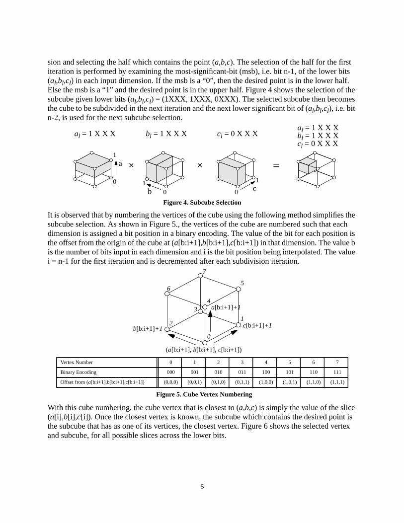
sion and selecting the half which contains the point (a,b,c). The selection of the half for the firstiteration is performed by examining the most-significant-bit (msb), i.e. bit n-1, of the lower bits(al,bl,cl) in each input dimension. If the msb is a “0”, then the desired point is in the lower half.Else the msb is a “1” and the desired point is in the upper half. Figure 4 shows the selection of thesubcube given lower bits (al,bl,cl) = (1XXX, 1XXX, 0XXX). The selected subcube then becomesthe cube to be subdivided in the next iteration and the next lower significant bit of (al,bl,cl), i.e. bitn-2, is used for the next subcube selection.

It is observed that by numbering the vertices of the cube using the following method simplifies thesubcube selection. As shown in Figure 5., the vertices of the cube are numbered such that eachdimension is assigned a bit position in a binary encoding. The value of the bit for each position isthe offset from the origin of the cube at (a[b:i+1],b[b:i+1],c[b:i+1]) in that dimension. The value bis the number of bits input in each dimension and i is the bit position being interpolated. The valuei = n-1 for the first iteration and is decremented after each subdivision iteration.

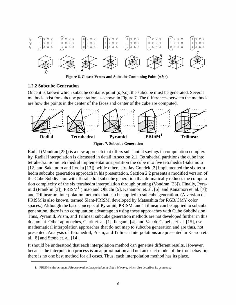
With this cube numbering, the cube vertex that is closest to (a,b,c) is simply the value of the slice(a[i],b[i],c[i]). Once the closest vertex is known, the subcube which contains the desired point isthe subcube that has as one of its vertices, the closest vertex. Figure 6 shows the selected vertexand subcube, for all possible slices across the lower bits.

a

b c

al = 1 X X X bl = 1 X X X cl = 0 X X Xal = 1 X X Xbl = 1 X X Xcl = 0 X X X

0

1

01

0

1

=

Figure 4. Subcube Selection

× ×

(a[b:i+1], b[b:i+1], c[b:i+1])

a[b:i+1]+1

b[b:i+1]+1 c[b:i+1]+1

0

12

34

56

7

Figure 5. Cube Vertex Numbering

Vertex Number 0 1 2 3 4 5 6 7

Binary Encoding 000 001 010 011 100 101 110 111

Offset from (a[b:i+1],b[b:i+1],c[b:i+1]) (0,0,0) (0,0,1) (0,1,0) (0,1,1) (1,0,0) (1,0,1) (1,1,0) (1,1,1)

6

1.2.2 Subcube GenerationOnce it is known which subcube contains point (a,b,c), the subcube must be generated. Severalmethods exist for subcube generation, as shown in Figure 7. The differences between the methodsare how the points in the center of the faces and center of the cube are computed.

Radial (Vondran [22]) is a new approach that offers substantial savings in computation complex-ity. Radial Interpolation is discussed in detail in section 2.1. Tetrahedral partitions the cube intotetrahedra. Some tetrahedral implementations partition the cube into five tetrahedra (Sakamoto[12] and Sakamoto and Itooka [13]), while others six. Jay Gondek [2] implemented the six tetra-hedra subcube generation approach in his presentation. Section 2.2 presents a modified version ofthe Cube Subdivision with Tetrahedral subcube generation that dramatically reduces the computa-tion complexity of the six tetrahedra interpolation through pruning (Vondran [23]). Finally, Pyra-mid (Franklin [3]), PRISM1 (Imao and Ohuchi [5], Kanamori et. al. [6], and Kanamori et. al. [7])and Trilinear are interpolation methods that can be applied to subcube generation. (A version ofPRISM is also known, termed Slant-PRISM, developed by Matsushita for RGB/CMY colorspaces.) Although the base concepts of Pyramid, PRISM, and Trilinear can be applied to subcubegeneration, there is no computation advantage in using these approaches with Cube Subdivision.Thus, Pyramid, Prism, and Trilinear subcube generation methods are not developed further in thisdocument. Other approaches, Clark et. al. [1], Ikegami [4], and Van de Capelle et. al. [15], usemathematical interpolation approaches that do not map to subcube generation and are thus, notpresented. Analysis of Tetrahedral, Prism, and Trilinear Interpolations are presented in Kasson et.al. [8] and Stone et. al. [14].

It should be understood that each interpolation method can generate different results. However,because the interpolation process is an approximation and not an exact model of the true behavior,there is no one best method for all cases. Thus, each interpolation method has its place.

1. PRISM is the acronym PRogrammable Interpolation by Small Memory, which also describes its geometry.

01 2 3

4 5 67

0 X X X0 X X X0 X X X








al:bl:cl:

Figure 6. Closest Vertex and Subcube Containing Point (a,b,c)

Radial Tetrahedral PRISM1 TrilinearFigure 7. Subcube Generation

Pyramid

7

2. Cube Subdivision Interpolation Methods

Presented in this section are new Cube Subdivision Interpolation methods based on Radial andTetrahedral subcube generation. The first is Radial Interpolation. As the name implies, thismethod is based on the Radial subcube generation. The second, Pruned Tetrahedral, exploits sev-eral key observations to reduce the complexity of the six tetrahedra interpolation approach. Alsopresented is a common implementation that can be used for both Radial and Pruned TetrahedralInterpolation. Finally, modifications to the Radial and Pruned Tetrahedral implementations arepresented that allow for these methods to interpolate when using a non-symmetric color lattice.

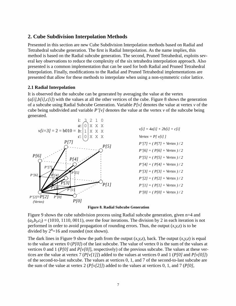
2.1 Radial InterpolationIt is observed that the subcube can be generated by averaging the value at the vertex(a[i],b[i],c[i]) with the values at all the other vertices of the cube. Figure 8 shows the generationof a subcube using Radial Subcube Generation. Variable P[v] denotes the value at vertex v of thecube being subdivided and variable P’[v] denotes the value at the vertex v of the subcube beinggenerated.

Figure 9 shows the cube subdivision process using Radial subcube generation, given n=4 and(al,bl,cl) = (1010, 1110, 0011), over the four iterations. The division by 2 in each iteration is notperformed in order to avoid propagation of rounding errors. Thus, the output (x,y,z) is to bedivided by 2n=16 and rounded (not shown).

The dark lines in Figure 9 show the path from the output (x,y,z), back. The output (x,y,z) is equalto the value at vertex 0 (P[0]) of the last subcube. The value of vertex 0 is the sum of the values atvertices 0 and 1 (P[0] and P[v[0]], respectively) of the previous subcube. The values at these ver-tices are the value at vertex 7 (P[v[1]]) added to the values at vertices 0 and 1 (P[0] and P[v[0]])of the second-to-last subcube. The values at vertices 0, 1, and 7 of the second-to-last subcube arethe sum of the value at vertex 2 (P[v[2]]) added to the values at vertices 0, 1, and 7 (P[0],

P’[2]=P[2]P[0]

P[1]P[3]

P[4]

P[5]

P[6]

P[7]

P’[0]

P’[1]P’[3]

P’[5]P’[4]

P’[7]

P’[6]

3 2 1 00 X X X1 X X X0 X X X

i:a:b:c:

v[i=3] = 2 = b010 = v[i] = 4a[i] + 2b[i] + c[i]

Vertex = P[ v[i] ]

P’[7] = ( P[7] + Vertex ) / 2

P’[6] = ( P[6] + Vertex ) / 2

P’[5] = ( P[5] + Vertex ) / 2

P’[4] = ( P[4] + Vertex ) / 2

P’[3] = ( P[3] + Vertex ) / 2

P’[2] = ( P[2] + Vertex ) / 2

P’[1] = ( P[1] + Vertex ) / 2

P’[0] = ( P[0] + Vertex ) / 2

(Vertex)

Figure 8. Radial Subcube Generation

8

P[v[0]], and P[v[1]]) of the third-to-last subcube. The values at vertices 0, 1, 2, and 7 of the third-to-last subcube are the sum of the value at vertex 6 (P[v[3]]) and vertices 0, 1, 7, and 2 (P[0],P[v[0]], P[v[1]], and P[v[2]]) of the cube input from the color table.

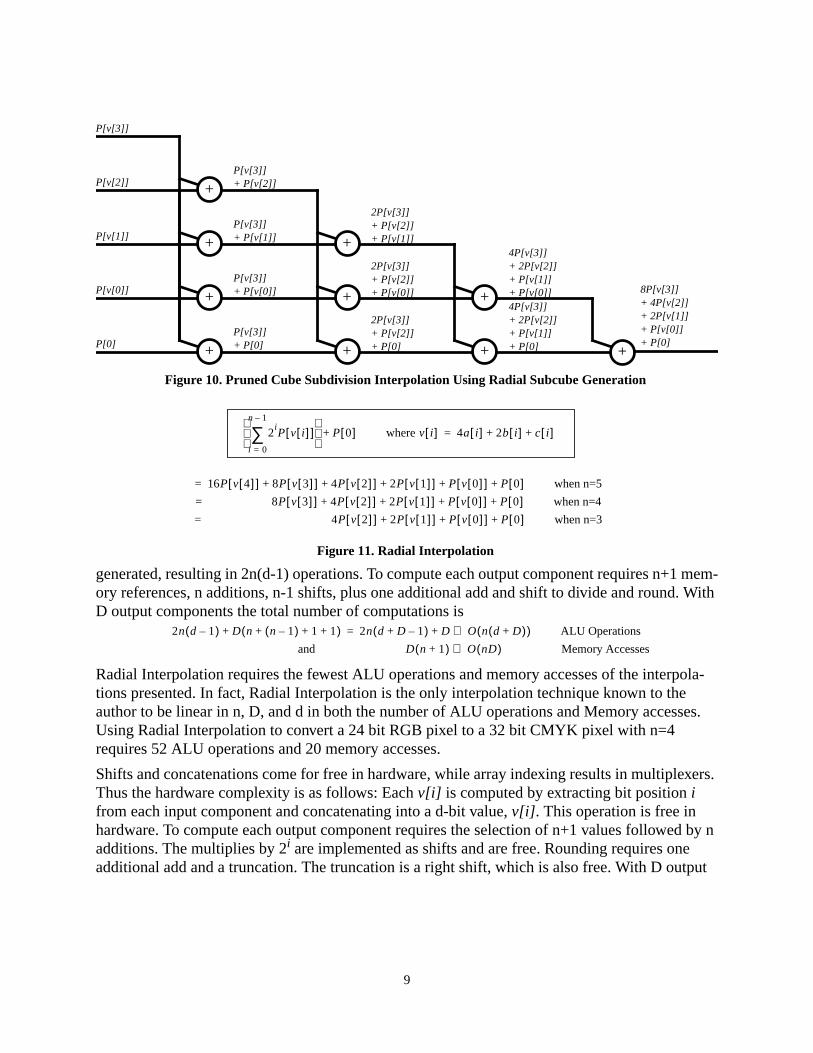
Note, only 10 of the 32 adders actually contribute to the output (x,y,z). In fact, only five of theeight vertices contribute to the output (vertices P[7], P[6], P[2], P[1] and P[0]). Figure 10 showsthe pruned implementation of the Cube Subdivision with Radial Cube Generation. Also shownare the values at each stage in the interpolation process.

As can be seen in Figure 10, the output can be computed directly (i.e. 8P[v[3]] + 4P[v[2]] +2P[v[1]] + P[v[0]] + P[0] ). A general equation can be developed to compute the output, and ispresented in Figure 11.

Given d input dimensions, D output dimensions and 2n values between coarse lattice points, thenumber of computations is: Each v[i] requires d-1 adds and d-1 shifts. There are n vertices v[i]

+

+

+

+

+

+

+

+

+

+

+

+

+

+

+

+

+

+

+

+

+

+

+

+

+

+

+

+

+

+

+

+

P[7]

P[6]

P[5]

P[4]

P[3]

P[2]

P[1]

P[0]

1 0 1 01 1 1 00 0 1 1

al:bl:cl:

1 0 1 01 1 1 00 0 1 1

v[3] = 6 v[2] = 2 v[1] = 7 v[0] = 1

1 0 1 01 1 1 00 0 1 1

1 0 1 01 1 1 00 0 1 1

(x,y,z)

Figure 9. Cube Subdivision Interpolation Using Radial Subcube Generation

9

generated, resulting in 2n(d-1) operations. To compute each output component requires n+1 mem-ory references, n additions, n-1 shifts, plus one additional add and shift to divide and round. WithD output components the total number of computations is

Radial Interpolation requires the fewest ALU operations and memory accesses of the interpola-tions presented. In fact, Radial Interpolation is the only interpolation technique known to theauthor to be linear in n, D, and d in both the number of ALU operations and Memory accesses.Using Radial Interpolation to convert a 24 bit RGB pixel to a 32 bit CMYK pixel with n=4requires 52 ALU operations and 20 memory accesses.

Shifts and concatenations come for free in hardware, while array indexing results in multiplexers.Thus the hardware complexity is as follows: Each v[i] is computed by extracting bit position ifrom each input component and concatenating into a d-bit value, v[i]. This operation is free inhardware. To compute each output component requires the selection of n+1 values followed by nadditions. The multiplies by 2i are implemented as shifts and are free. Rounding requires oneadditional add and a truncation. The truncation is a right shift, which is also free. With D output

+

8P[v[3]]+ 4P[v[2]]+ 2P[v[1]]+ P[v[0]]+ P[0]

4P[v[3]]+ 2P[v[2]]+ P[v[1]]+ P[0]

4P[v[3]]+ 2P[v[2]]+ P[v[1]]+ P[v[0]]

2P[v[3]]+ P[v[2]]+ P[v[0]]

2P[v[3]]+ P[v[2]]+ P[v[1]]

2P[v[3]]+ P[v[2]]+ P[0]

P[v[3]]+ P[v[1]]

P[v[3]]+ P[v[2]]

P[v[3]]+ P[v[0]]

P[v[3]]+ P[0]

P[v[1]]

P[v[2]]

P[v[0]]

P[0]

P[v[3]]

+

+

+

+

+

+

+

+

+

Figure 10. Pruned Cube Subdivision Interpolation Using Radial Subcube Generation

2iP v i[ ][ ]

i 0=

n 1–

∑

P 0[ ]+ where v i[ ] 4a i[ ] 2b i[ ] c i[ ]+ +=

16P v 4[ ][ ] 8P v 3[ ][ ] 4P v 2[ ][ ] 2P v 1[ ][ ] P v 0[ ][ ] P 0[ ]+ + + + + when n=5=

8P v 3[ ][ ] 4P v 2[ ][ ] 2P v 1[ ][ ] P v 0[ ][ ] P 0[ ]+ + + += when n=4

4P v 2[ ][ ] 2P v 1[ ][ ] P v 0[ ][ ] P 0[ ]+ + += when n=3

Figure 11. Radial Interpolation

2n d 1–( ) D n n 1–( ) 1 1+ + +( )+ 2n d D 1–+( ) D+ O n d D+( )( )⇒= ALU Operations

and D n 1+( ) O nD( )⇒ Memory Accesses

10

components the total number of hardware elements is

Figure 12 presents a C code implementation of Radial Interpolation. Note, the presented imple-mentation is designed to minimize control flow dependencies, i.e. branches, which are becomingmore costly in high performance architectures. It is understood that implementations can bedeveloped to minimize other aspects, e.g. memory accesses, etc.. The implementation operates asfollows: Passed in is an array of input components, a color table pointer array, and an array of out-put components. Each input component is checked if it is the maximum value (i.e. 255). Remem-ber that the last point of each dimension is stored in the color table to allow for interpolationbetween the last point that is a multiple of 2n and the final value in the color space. It can beshown that the segment from the last multiple of 2n and the final value has 2n-1 steps instead of 2n,which the interpolation process assumes. Therefore, when the maximum value is observed, itsvalue is incremented by one to assure the final point is reached.

Next, the indices into the color table are generated. The indices include the origin (i.e. point 0),v[0], v[1], v[2], and v[3]. Note, in this implementation, the values, origin, v0, v1, v2, and v3, areactually the indices into the color table and not just the offset from the origin. This was done tosimplify the presented implementation. Once the indices are generated, the output components are

D n 1+( ) O nD( )⇒ Adders

D n 1+( ) O nD( )⇒ Multiplexers 2d:1( )

#define C_INC 1#define B_INC C_INC*17#define A_INC B_INC*17#define TABLE_INC A_INC*17/******************************************//** radial_interpolation() **//******************************************/void radial_interpolation(unsigned char input[],unsigned char table[][TABLE_INC], unsigned char output[]){

register int origin, v0, v1, v2, v3 ;register int a, b, c ;register int x, y, z ;

/**************************************//* Snap max value to last table value *//**************************************/a = ( input[0] == 0x0ff ) ? 0x100 : (int) input[0] ;b = ( input[1] == 0x0ff ) ? 0x100 : (int) input[1] ;c = ( input[2] == 0x0ff ) ? 0x100 : (int) input[2] ;

/***************************************//* Compute Indexes into table *//***************************************/origin = A_INC*(a >> 4) + B_INC*(b >> 4) + (c >> 4) ;v0 = origin + A_INC*( (a & 0x01) )

+ B_INC*( (b & 0x01) ) + (c & 0x01 ) ;

v1 = origin + A_INC*( (a & 0x02) >> 1 ) + B_INC*( (b & 0x02) >> 1 ) + (c & 0x02 ) >> 1) ;

v2 = origin + A_INC*( (a & 0x04) >> 2 ) + B_INC*( (b & 0x04) >> 2 ) + (c & 0x04) >> 2) ;

v3 = origin + A_INC*( (a & 0x08) >> 3 ) + B_INC*( (b & 0x08) >> 3 ) + (c & 0x08) >> 3 ) ;

/*************//* Compute x *//*************/x = ( ( (int) table[0][origin] + (int) table[0][v0] + ( (int) table[0][v1] << 1 ) + ( (int) table[0][v2] << 2 ) + ( (int) table[0][v3] << 3 ) + 0x08 ) >> 4 ) ; /* Round */

/*************//* Compute y *//*************/y = ( ( (int) table[1][origin] + (int) table[1][v0] + ( (int) table[1][v1] << 1 ) + ( (int) table[1][v2] << 2 ) + ( (int) table[1][v3] << 3 ) + 0x08 ) >> 4 ) ; /* Round */

/*************//* Compute z *//*************/z = ( ( (int) table[2][origin] + (int) table[2][v0] + ( (int) table[2][v1] << 1 ) + ( (int) table[2][v2] << 2 ) + ( (int) table[2][v3] << 3 ) + 0x08 ) >> 4 ) ; /* Round */

output[0] = (char) x ;output[1] = (char) y ;output[2] = (char) z ;

}

Figure 12. Radial Interpolation C Implementation with n=4

11

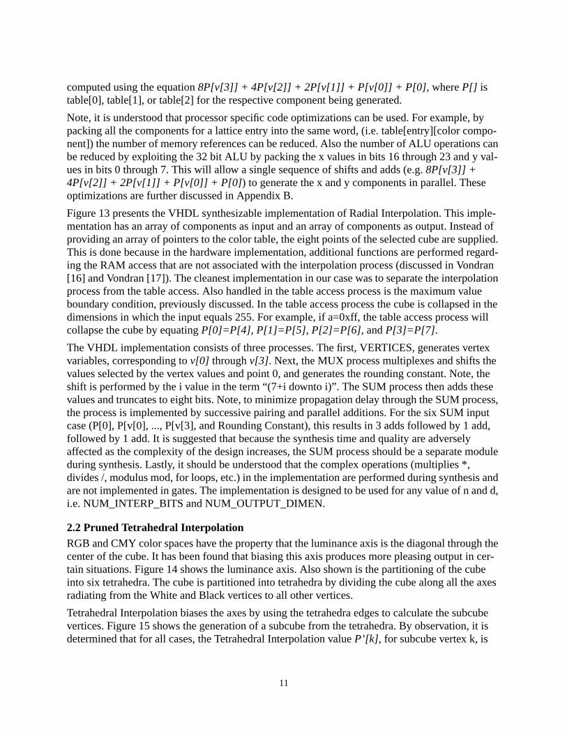
computed using the equation 8P[v[3]] + 4P[v[2]] + 2P[v[1]] + P[v[0]] + P[0], where P[] istable[0], table[1], or table[2] for the respective component being generated.

Note, it is understood that processor specific code optimizations can be used. For example, bypacking all the components for a lattice entry into the same word, (i.e. table[entry][color compo-nent]) the number of memory references can be reduced. Also the number of ALU operations canbe reduced by exploiting the 32 bit ALU by packing the x values in bits 16 through 23 and y val-ues in bits 0 through 7. This will allow a single sequence of shifts and adds (e.g. 8P[v[3]] +4P[v[2]] + 2P[v[1]] + P[v[0]] + P[0]) to generate the x and y components in parallel. Theseoptimizations are further discussed in Appendix B.

Figure 13 presents the VHDL synthesizable implementation of Radial Interpolation. This imple-mentation has an array of components as input and an array of components as output. Instead ofproviding an array of pointers to the color table, the eight points of the selected cube are supplied.This is done because in the hardware implementation, additional functions are performed regard-ing the RAM access that are not associated with the interpolation process (discussed in Vondran[16] and Vondran [17]). The cleanest implementation in our case was to separate the interpolationprocess from the table access. Also handled in the table access process is the maximum valueboundary condition, previously discussed. In the table access process the cube is collapsed in thedimensions in which the input equals 255. For example, if a=0xff, the table access process willcollapse the cube by equating P[0]=P[4], P[1]=P[5], P[2]=P[6], and P[3]=P[7].

The VHDL implementation consists of three processes. The first, VERTICES, generates vertexvariables, corresponding to v[0] through v[3]. Next, the MUX process multiplexes and shifts thevalues selected by the vertex values and point 0, and generates the rounding constant. Note, theshift is performed by the i value in the term “(7+i downto i)”. The SUM process then adds thesevalues and truncates to eight bits. Note, to minimize propagation delay through the SUM process,the process is implemented by successive pairing and parallel additions. For the six SUM inputcase (P[0], P[v[0], ..., P[v[3], and Rounding Constant), this results in 3 adds followed by 1 add,followed by 1 add. It is suggested that because the synthesis time and quality are adverselyaffected as the complexity of the design increases, the SUM process should be a separate moduleduring synthesis. Lastly, it should be understood that the complex operations (multiplies *,divides /, modulus mod, for loops, etc.) in the implementation are performed during synthesis andare not implemented in gates. The implementation is designed to be used for any value of n and d,i.e. NUM_INTERP_BITS and NUM_OUTPUT_DIMEN.

2.2 Pruned Tetrahedral InterpolationRGB and CMY color spaces have the property that the luminance axis is the diagonal through thecenter of the cube. It has been found that biasing this axis produces more pleasing output in cer-tain situations. Figure 14 shows the luminance axis. Also shown is the partitioning of the cubeinto six tetrahedra. The cube is partitioned into tetrahedra by dividing the cube along all the axesradiating from the White and Black vertices to all other vertices.

Tetrahedral Interpolation biases the axes by using the tetrahedra edges to calculate the subcubevertices. Figure 15 shows the generation of a subcube from the tetrahedra. By observation, it isdetermined that for all cases, the Tetrahedral Interpolation value P’[k], for subcube vertex k, is

12

equal to the average of the subdivided cube values P[k & v[i]] and P[k | v[i]]. Note, characters“&” and “|” denote the bitwise AND and OR operations, respectively.

Figure 16 shows the Pruned Tetrahedral Interpolation for n=4. P’[] denotes the values of the sub-

Figure 13. Radial Interpolation VHDL Implementation with n=NUM_INTERP_BITS

------------------------------------------------------- Radial Interpolation. -------------------------------------------------------entity radial isport ( -- Input Pixel (a,b,c) -- input: in INPUT_ARRAY ; -- Vertex Points of Cube from Color Table -- point: in POINT_ARRAY ; -- Output Pixel (x,y,z) -- output: out OUTPUT_ARRAY) ;end radial ;

---------------------------------------------architecture radialrtl of radial is---------------------------------------------

signal vertex: VERTEX_ARRAY ; signal point_value: POINT_VALUE_ARRAY ;

begin

----------------------------------------------------------- Compute selected vertices from slices across input.---------------------------------------------------------VERTICIES: process ( input )begin ------------------------------------------------ -- For each slice across the input lower bits -- ------------------------------------------------ for i in NUM_INTERP_BITS-1 downto 0 loop vertex(i) <= input(0)(i) & input(1)(i) & input(2)(i); end loop ;end process ;

--------------------------------------------------- Select the values of vertices to be used by ---- interpolation. The last two vertices are ---- always point(0) and the rounding constant. ---------------------------------------------------MUX: process ( vertex, point )begin ------------------------------- -- For each output dimension -- ------------------------------- for d in 0 to NUM_OUTPUT_DIMEN-1 loop ---------------- -- Initialize -- ---------------- point_value(d) <= (others => (others => ‘0’));

------------------------------------------ -- point_value( 0 : NUM_INTERP_BITS-1 ) -- ------------------------------------------ for i in 0 to NUM_INTERP_BITS-1 loop case vertex(i) is

when “000” => point_value(d)(i)(7+i downto i) <= point(d)(0) ; when “001” => point_value(d)(i)(7+i downto i <= point(d)(1) ;

when “010” => point_value(d)(i)(7+i downto i) <= point(d)(2) ;



when “101” => point_value(d)(i)(7+i downto i) <= point(d)(5);

when “110” => point_value(d)(i)(7+i downto i) <= point(d)(6);

when others => point_value(d)(i)(7+i downto i) <= point(d)(7); end case ;

----------------- -- point(d)(0) -- ----------------- point_value(d)(NUM_INTERP_BITS)(7 downto 0) <= point(d)(0) ; ----------------------- -- Rounding constant -- ----------------------- point_value(d)(NUM_INTERP_BITS+1) (NUM_INTERP_BITS-1) <= ‘1’ ; end loop ; end loop ;end process ;

------------------------------------------------------- SUM adds the selected vertices values and trun- ---- cates to eight bits. The process is implemented ---- to minimize time by successive pairing and ---- adding. -------------------------------------------------------SUM: process ( point_value ) variable temp: POINT_VALUES ; variable bound: INTEGER ;begin ------------------------------- -- For each output dimension -- ------------------------------- for d in 0 to NUM_OUTPUT_DIMEN-1 loop -------------------------------- -- Initialize temp and bound. -- -------------------------------- temp := point_value(d) ; bound := NUM_INTERP_BITS + 2 ; --------------------------------------------- -- Loop for ceil(log2(NUM_INTERP_BITS-1)). -- --------------------------------------------- for i in 0 to NUM_INTERP_BITS-1 loop --------------------------------------- -- Pair temp array elements and add. -- --------------------------------------- for j in 0 to (NUM_INTERP_BITS/2) loop ------------------------------- -- Step 1: Move temp(even’s) -- ------------------------------- if ( 2*j < bound ) then temp(j) := temp(2*j) ; else temp(j) := (others => ‘0’) ; end if ; ----------------------------- -- Step 2: Add temp(odd’s) -- ----------------------------- if ( (2*j)+1 < bound ) then temp(j) := temp(j) + temp((2*j)+1); else temp(j) := temp(j) ; end if ; end loop ; ---------------------------------- -- Set bound for next iteration -- ---------------------------------- bound := ( bound / 2 ) + ( bound mod 2 ) ; end loop ; ---------------------- -- Truncate output. -- ---------------------- output(d) <= temp(0)(7+NUM_INTERP_BITS downto NUM_INTERP_BITS) ; end loop ;end process ;

---------------------------------------------------------end radialrtl;---------------------------------------------------------

13

cube vertices after the first subdivision iteration. P’’[] denotes the values of the subcube verticesafter the second subdivision iteration. And P’’’[] and P’’’’[] denote the values of the vertices afterthe third and fourth iterations, respectively. Note, the division by 2 in each iteration is not per-formed in order to avoid propagation of rounding errors. Thus the output (x,y,z) is to be divided by2n=16 and rounded (not shown).

Given d input dimensions, D output dimensions and 2n values between coarse lattice points, the

Black

White

Blue

Green

Cyan

RedMagenta

Yellow

Lum

inan

ce

Figure 14. Luminance Axis in RGB/CMY Color Space and Tetrahedral Cube Partitioning

P’[2]=P[2]P[0]

P[1]P[3]

P[4]

P[5]

P[6]

P[7]

P’[0]

P’[1]P’[3]

P’[5]P’[4]

P’[7]

P’[6]

(Vertex)

P’[2]=P[2]P[0]

P[7]

P’[0]

P’[6]

(Vertex)

P[3]

P’[1]P’[3]

P’[5]P’[4]

P’[7]

P’[2]=P[2]P[0]

P[6]

P[7]

P’[0]

P’[6]

(Vertex)

P[3]

P’[1]P’[3]

P’[5]P’[4]

P’[7]

Figure 15. Tetrahedral Subcube Generation

P’[7] = ( P[v[i] & 7] + P[v[i] | 7] ) / 2

= ( P[v[i]] + P[7] ) / 2

P’[6] = ( P[v[i] & 6] + P[v[i] | 6] ) / 2

P’[5] = ( P[v[i] & 5] + P[v[i] | 5] ) / 2

P’[4] = ( P[v[i] & 4] + P[v[i] | 4] ) / 2

P’[3] = ( P[v[i] & 3] + P[v[i] | 3] ) / 2

P’[2] = ( P[v[i] & 2] + P[v[i] | 2] ) / 2

P’[1] = ( P[v[i] & 1] + P[v[i] | 1] ) / 2

P’[0] = ( P[v[i] & 0] + P[v[i] | 0] ) / 2

= ( P[0] + P[v[i]] ) / 2

where v[i] = 4a[i] + 2b[i] + c[i]

14

number of computations is: Each v[i] requires d adds and d-1 shifts. There are n vertices v[i] gen-erated, resulting in n(2d-1) operations. From this, 2n memory indexes are computed, some as sim-ple as “0” and “v[n-1]”, while others are a series of ANDs and ORs. One form of reduction is thatcommon subexpressions exists in the index computations (e.g. “v[1] & v[0]” is used in manyexpressions in the example). The number of logic operations to compute the indices is equal to

As can be seen in Figure 16, 2n-1 additions are used. One additional add and shift is needed peroutput component to divide and round, totaling (2n-1)+1+1 = 2n+1. Also in Figure 16, 2n memoryreferences are shown. However, Pruned Tetrahedral Interpolation can be implemented such that acap is placed on the number of memory accesses at the number of vertices of the cube (2d verticesare on the cube). Thus, the minimum of the two is used, i.e. min(2d, 2n). With D output compo-nents the total number of computations is

Using Pruned Tetrahedral Interpolation to convert a 24 bit RGB pixel to a 32 bit CMYK pixelwith n=4 requires 110 ALU operations and 32 memory accesses. Clearly, biasing the luminanceaxis comes at the cost of more operations (unbiased Radial Cube Subdivision Interpolation

Figure 16. Pruned Tetrahedral Interpolation

+

+

+

+

+

+

+

+

+

+

+

+

+

+

+

P[0]

P[v[3]]

P[v[3] | v[2]]

P[v[3] & v[2]]

P[v[3] | (v[2] | v[1])]

P[v[3] & (v[2] | v[1])]

P[v[3] | (v[2] & v[1])]

P[v[3] & (v[2] & v[1])]

P[v[3] | (v[2] | (v[1] | v[0]))]

P[v[3] & (v[2] | (v[1] | v[0]))]

P[v[3] | (v[2] & (v[1] | v[0]))]

P[v[3] & (v[2] & (v[1] | v[0]))]

P[v[3] | (v[2] | (v[1] & v[0]))]

P[v[3] & (v[2] | (v[1] & v[0]))]

P[v[3] | (v[2] & (v[1] & v[0]))]

P[v[3] & (v[2] & (v[1] & v[0]))]

P’’’’[0] = (x,y,z)

P’’’[0]

P’’’[v[0]]

P’’[0]

P’’[v[1]]

P’’[v[1] | v[0]]

P’’[v[1] & v[0]]

P’[0]

P’[v[2]]

P’[v[2] | v[1]]

P’[v[2] & v[1]]

P’[v[2] | (v[1] | v[0])]

P’[v[2] & (v[1] | v[0])]

P’[v[2] | (v[1] & v[0])]

P’[v[2] & (v[1] & v[0])]Where v[i] = 4a[i] + 2b[i] + c[i]

2 2i

1–( )i 1=

n 1–

∑ 2 1 3 7 …+ + +( )=

n 2d 1–( ) 2 2i

1–( )i 1=

n 1–

∑ D 2n

1+( )+ + O nd 2nD+( )⇒ ALU Operations

and D min 2d

2n,( )( ) O D min 2

d2

n,( )( )( )⇒ Memory Accesses

15

requires a total of 52 ALU operations and 20 memory accesses for the same conversion).

Shifts and concatenations come for free in hardware, while array indexing results in multiplexers.Thus, the hardware complexity is as follows: Each v[i] is computed by extracting bit position ifrom each input component and concatenating into a d-bit value, v[i]. The number of AND/ORgates to compute the indices is equal to

To compute each output component requires the selection of 2n-1 values followed by 2n-1 addi-tions. Rounding requires one additional add and a truncation. The truncation is a right shift, whichis free. With D output components the total number of hardware elements is

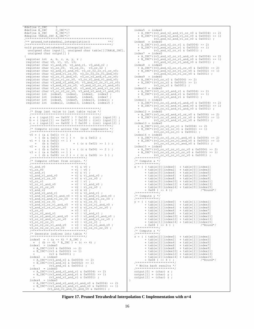
Figure 17 presents the C implementation for Pruned Tetrahedral Interpolation. The implementa-tion operates as follows: Passed in is an array of input components, an array of color table point-ers, and an array of output components. Each input component is snapped to the last table value ifthe input is the maximum value (i.e. 255) in that dimension. Next, the selected vertices, v0through v3, and indices into the color table are generated. Finally the table is accessed and the val-ues summed, rounded and truncated to eight bits.

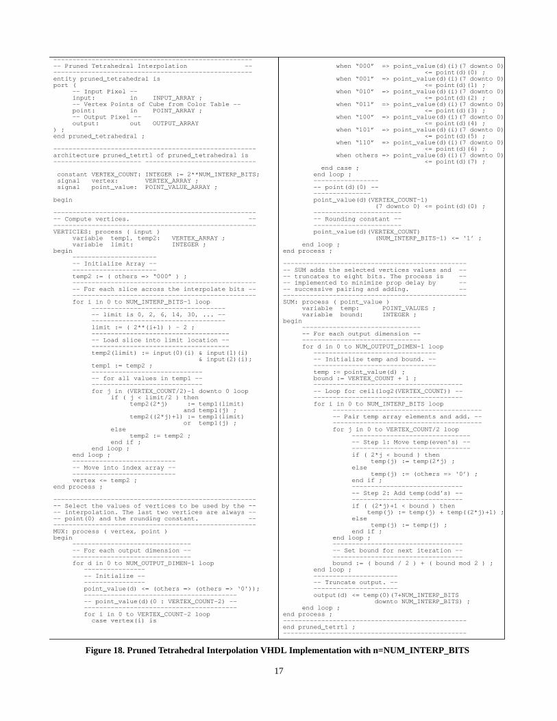
Figure 18 presents the VHDL implementation of Pruned Tetrahedral Interpolation. The VHDLimplementation consists of three processes. The first, VERTICES, generates the vertex variablesand performs the bitwise AND and OR operations to produce the vertex selections for the MUXprocess. The MUX process multiplexes the values selected by the vertex values and point 0, andgenerates the rounding constant. The SUM process then adds these values and truncates to eightbits. Note, it should be understood that the complex operations (multiplies *, divides /, modulusmod, for loops, etc.) in the implementation are performed during synthesis and are not imple-mented in gates.

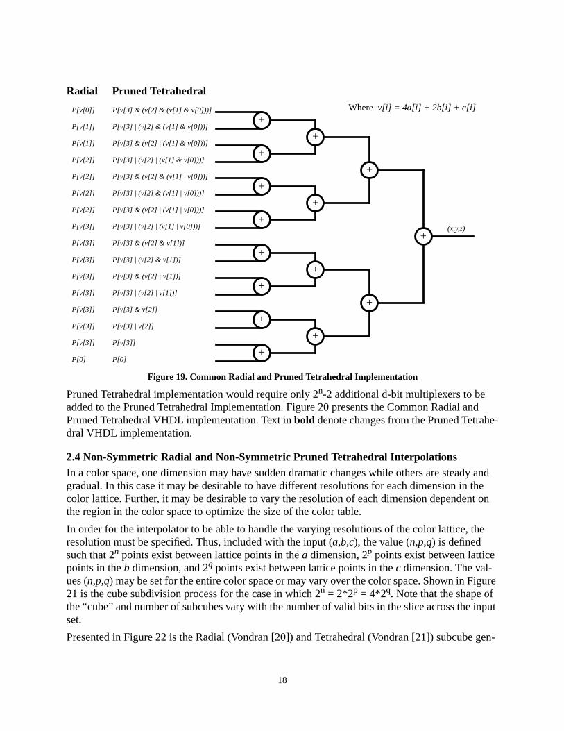
2.3 Common Radial and Pruned Tetrahedral ImplementationA user may wish to use Pruned Tetrahedral for conversions of RGB and CMY pixels, and RadialInterpolation for all others (CieLab, LUV, YCbCr, etc.). In software this is easily done by calling adifferent routine. Separate implementations in hardware, however, mean separate logic that maybe idle when the other interpolation is in use. Thus it is desirable to develop a common implemen-tation that can be used for both Radial or Pruned Tetrahedral Interpolation. Figure 19 (Vondran[19]) presents the common implementation for n=4.

Notice that the difference between the two types of interpolation is the index of the vertices.Because the number of bits of v[] is generally less than the number of bits of variable P[], it isbetter to multiplex the indices prior to the memory access. Also note that the last two values(P[v[3]] and P[0]) are the same and will be for all values of n. Thus, a common Radial and

d 2 2i

1–( )i 1=

n 1–

∑

2d 1 3 7 …+ + +( )=

D 2n

1–( ) 1+( ) D 2n( ) O 2

nD( )⇒= Adders

D 2n

1–( ) O 2nD( )⇒ Multiplexers 2

d:1( )

d 2 2i

1–( )i 1=

n 1–

∑

O 2nd( )⇒ Additional AND/OR Gates

16

Figure 17. Pruned Tetrahedral Interpolation C Implementation with n=4

#define C_INC 1#define B_INC C_INC*17#define A_INC B_INC*17#degine TABLE_INC A_INC*17/*************************************************//** pruned_tetrahedral_interpolation() **//*************************************************/void pruned_tetrahedral_interpolation(unsigned char input[], unsigned char table[][TABLE_INC],

unsigned char output[] ){ register int a, b, c, x, y, z ; register char v0, v1, v2, v3; register char v1_and_v0, v2_and_v1, v3_and_v2 ; register char v1_or_v0, v2_or_v1, v3_or_v2 ; register char v2_and_v1_and_v0, v3_or_v2_or_v1_or_v0; register char v2_and_v1_or_v0, v3_or_v2_or_v1_and_v0; register char v2_or_v1_and_v0, v3_or_v2_and_v1_or_v0; register char v2_or_v1_or_v0, v3_or_v2_and_v1_and_v0; register char v3_and_v2_and_v0, v3_and_v2_or_v1_or_v0; register char v3_and_v2_or_v0, v3_and_v2_or_v1_and_v0; register char v3_or_v2_and_v0, v3_and_v2_and_v1_or_v0; register char v3_or_v2_or_v0, v3_and_v2_and_v1_and_v0; register int index0, index1, index2, index3 ; register int index4, index5, index6, index7 ; register int index8, index9, index10, index11 ; register int index12, index13, index14, index15 ;

/***************************************/ /* Snap last value to last table value */ /***************************************/ a = ( input[0] == 0x0ff ) ? 0x100 : (int) input[0] ; b = ( input[1] == 0x0ff ) ? 0x100 : (int) input[1] ; c = ( input[2] == 0x0ff ) ? 0x100 : (int) input[2] ; /**********************************************/ /* Compute slices across the input components */ /**********************************************/ v0 = ( (a & 0x01) << 2 ) + ( (b & 0x01) << 1 ) + (c & 0x01) ; v1 = ( (a & 0x02) << 1 ) + (b & 0x02) + ( (c & 0x02) >> 1 ) ; v2 = (a & 0x04) + ( (b & 0x04) >> 1 ) + ( (c & 0x04) >> 2 ) ; v3 = ( (a & 0x08) >> 1 ) + ( (b & 0x08) >> 2 ) + ( (c & 0x08) >> 3 ) ; /*******************************/ /* Compute offset from origin. */ /*******************************/ v1_and_v0 = v1 & v0 ; v1_or_v0 = v1 | v0 ; v2_and_v1 = v2 & v1 ; v2_and_v1_and_v0 = v2 & v1_and_v0 ; v2_and_v1_or_v0 = v2 & v1_or_v0 ; v2_or_v1 = v2 | v1 ; v2_or_v1_and_v0 = v2 | v1_and_v0 ; v2_or_v1_or_v0 = v2 | v1_or_v0 ; v3_and_v2 = v3 & v2 ; v3_and_v2_and_v1 = v3 & v2_and_v1 ; v3_and_v2_and_v1_and_v0 = v3 & v2_and_v1_and_v0 ; v3_and_v2_and_v1_or_v0 = v3 & v2_and_v1_or_v0 ; v3_and_v2_or_v1 = v3 & v2_or_v1 ; v3_and_v2_or_v1_and_v0 = v3 & v2_or_v1_and_v0 ; v3_and_v2_or_v1_or_v0 = v3 & v2_or_v1_or_v0 ; v3_or_v2 = v3 | v2 ; v3_or_v2_and_v1 = v3 | v2_and_v1 ; v3_or_v2_and_v1_and_v0 = v3 | v2_and_v1_and_v0 ; v3_or_v2_and_v1_or_v0 = v3 | v2_and_v1_or_v0 ; v3_or_v2_or_v1 = v3 | v2_or_v1 ; v3_or_v2_or_v1_and_v0 = v3 | v2_or_v1_and_v0 ; v3_or_v2_or_v1_or_v0 = v3 | v2_or_v1_or_v0 ; /*******************************/ /* Generate indices into table */ /*******************************/ index0 = ( (a >> 4) * A_INC ) + ( (b >> 4) * B_INC ) + (c >> 4) ; index1 = index0 + A_INC*((v3 & 0x0004) >> 2) + B_INC*((v3 & 0x0002) >> 1) + (v3 & 0x0001) ; index2 = index0 + A_INC*((v3_and_v2 & 0x0004) >> 2) + B_INC*((v3_and_v2 & 0x0002) >> 1) + (v3_and_v2 & 0x0001) ; index3 = index0 + A_INC*((v3_and_v2_and_v1 & 0x0004) >> 2) + B_INC*((v3_and_v2_and_v1 & 0x0002) >> 1) + (v3_and_v2_and_v1 & 0x0001) ; index4 = index0 + A_INC*((v3_and_v2_and_v1_and_v0 & 0x0004) >> 2) + B_INC*((v3_and_v2_and_v1_and_v0 & 0x0002) >> 1) + (v3_and_v2_and_v1_and_v0 & 0x0001) ;

index5 = index0 + A_INC*((v3_and_v2_and_v1_or_v0 & 0x0004) >> 2) + B_INC*((v3_and_v2_and_v1_or_v0 & 0x0002) >> 1) + (v3_and_v2_and_v1_or_v0 & 0x0001) ; index6 = index0 + A_INC*((v3_and_v2_or_v1 & 0x0004) >> 2) + B_INC*((v3_and_v2_or_v1 & 0x0002) >> 1) + (v3_and_v2_or_v1 & 0x0001) ; index7 = index0 + A_INC*((v3_and_v2_or_v1_and_v0 & 0x0004) >> 2) + B_INC*((v3_and_v2_or_v1_and_v0 & 0x0002) >> 1) + (v3_and_v2_or_v1_and_v0 & 0x0001) ; index8 = index0 + A_INC*((v3_and_v2_or_v1_or_v0 & 0x0004) >> 2) + B_INC*((v3_and_v2_or_v1_or_v0 & 0x0002) >> 1) + (v3_and_v2_or_v1_or_v0 & 0x0001) ; index9 = index0 + A_INC*((v3_or_v2 & 0x0004) >> 2) + B_INC*((v3_or_v2 & 0x0002) >> 1) + (v3_or_v2 & 0x0001) ; index10 = index0 + A_INC*((v3_or_v2_and_v1 & 0x0004) >> 2) + B_INC*((v3_or_v2_and_v1 & 0x0002) >> 1) + (v3_or_v2_and_v1 & 0x0001) ; index11 = index0 + A_INC*((v3_or_v2_and_v1_and_v0 & 0x0004) >> 2) + B_INC*((v3_or_v2_and_v1_and_v0 & 0x0002) >> 1) + (v3_or_v2_and_v1_and_v0 & 0x0001) ; index12 = index0 + A_INC*((v3_or_v2_and_v1_or_v0 & 0x0004) >> 2) + B_INC*((v3_or_v2_and_v1_or_v0 & 0x0002) >> 1) + (v3_or_v2_and_v1_or_v0 & 0x0001) ; index13 = index0 + A_INC*((v3_or_v2_or_v1 & 0x0004) >> 2) + B_INC*((v3_or_v2_or_v1 & 0x0002) >> 1) + (v3_or_v2_or_v1 & 0x0001) ; index14 = index0 + A_INC*((v3_or_v2_or_v1_and_v0 & 0x0004) >> 2) + B_INC*((v3_or_v2_or_v1_and_v0 & 0x0002) >> 1) + (v3_or_v2_or_v1_and_v0 & 0x0001) ; index15 = index0 + A_INC*((v3_or_v2_or_v1_or_v0 & 0x0004) >> 2) + B_INC*((v3_or_v2_or_v1_or_v0 & 0x0002) >> 1) + (v3_or_v2_or_v1_or_v0 & 0x0001) ; /*************/ /* Compute x */ /*************/ x = ( ( table[0][index0] + table[0][index1] + table[0][index2] + table[0][index3] + table[0][index4] + table[0][index5] + table[0][index6] + table[0][index7] + table[0][index8] + table[0][index9] + table[0][index10] + table[0][index11] + table[0][index12] + table[0][index13] + table[0][index14] + table[0][index15] + 0x08 ) >> 4 ); /*Round*/ /*************/ /* Compute y */ /*************/ y = ( ( table[1][index0] + table[1][index1] + table[1][index2] + table[1][index3] + table[1][index4] + table[1][index5] + table[1][index6] + table[1][index7] + table[1][index8] + table[1][index9] + table[1][index10] + table[1][index11] + table[1][index12] + table[1][index13] + table[1][index14] + table[1][index15] + 0x08 ) >> 4 ) ; /*Round*/ /*************/ /* Compute z */ /*************/ z = ( ( table[2][index0] + table[2][index1] + table[2][index2] + table[2][index3] + table[2][index4] + table[2][index5] + table[2][index6] + table[2][index7] + table[2][index8] + table[2][index9] + table[2][index10] + table[2][index11] + table[2][index12] + table[2][index13] + table[2][index14] + table[2][index15] + 0x08 ) >> 4 ) ; /*Round*/ /**********************/ * Write back results */ /**********************/ output[0] = (char) x ; output[1] = (char) y ; output[2] = (char) z ;}

17

Figure 18. Pruned Tetrahedral Interpolation VHDL Implementation with n=NUM_INTERP_BITS

------------------------------------------------------ Pruned Tetrahedral Interpolation ------------------------------------------------------entity pruned_tetrahedral isport ( -- Input Pixel -- input: in INPUT_ARRAY ; -- Vertex Points of Cube from Color Table -- point: in POINT_ARRAY ; -- Output Pixel -- output: out OUTPUT_ARRAY) ;end pruned_tetrahedral ;

-----------------------------------------------------architecture pruned_tetrtl of pruned_tetrahedral is----------------------- -----------------------------

constant VERTEX_COUNT: INTEGER := 2**NUM_INTERP_BITS; signal vertex: VERTEX_ARRAY ; signal point_value: POINT_VALUE_ARRAY ;

begin

------------------------------------------------------- Compute vertices. -------------------------------------------------------VERTICIES: process ( input ) variable temp1, temp2: VERTEX_ARRAY ; variable limit: INTEGER ;begin ---------------------- -- Initialize Array -- ---------------------- temp2 := ( others => “000” ) ; ------------------------------------------------ -- For each slice across the interpolate bits -- ------------------------------------------------ for i in 0 to NUM_INTERP_BITS-1 loop ----------------------------------- -- limit is 0, 2, 6, 14, 30, ... -- ----------------------------------- limit := ( 2**(i+1) ) - 2 ; ------------------------------------ -- Load slice into limit location -- ------------------------------------ temp2(limit) := input(0)(i) & input(1)(i) & input(2)(i); temp1 := temp2 ; ----------------------------- -- for all values in temp1 -- ----------------------------- for j in (VERTEX_COUNT/2)-1 downto 0 loop if ( j < limit/2 ) then temp2(2*j) := temp1(limit) and temp1(j) ; temp2((2*j)+1) := temp1(limit) or temp1(j) ; else temp2 := temp2 ; end if ; end loop ; end loop ; --------------------------- -- Move into index array -- --------------------------- vertex <= temp2 ;end process ;

------------------------------------------------------- Select the values of vertices to be used by the ---- interpolation. The last two vertices are always ---- point(0) and the rounding constant. -------------------------------------------------------MUX: process ( vertex, point )begin ------------------------------- -- For each output dimension -- ------------------------------- for d in 0 to NUM_OUTPUT_DIMEN-1 loop ---------------- -- Initialize -- ---------------- point_value(d) <= (others => (others => ‘0’)); ---------------------------------------- -- point_value(d)(0 : VERTEX_COUNT-2) -- ---------------------------------------- for i in 0 to VERTEX_COUNT-2 loop case vertex(i) is

when “000” => point_value(d)(i)(7 downto 0) <= point(d)(0) ;







when others => point_value(d)(i)(7 downto 0) <= point(d)(7) ; end case ; end loop ; ----------------- -- point(d)(0) -- --------------- point_value(d)(VERTEX_COUNT-1) (7 downto 0) <= point(d)(0) ; ----------------------- -- Rounding constant -- ----------------------- point_value(d)(VERTEX_COUNT) (NUM_INTERP_BITS-1) <= ‘1’ ; end loop ;end process ;

-------------------------------------------------- SUM adds the selected vertices values and ---- truncates to eight bits. The process is ---- implemented to minimize prop delay by ---- successive pairing and adding. --------------------------------------------------SUM: process ( point_value ) variable temp: POINT_VALUES ; variable bound: INTEGER ;begin ------------------------------- -- For each output dimension -- ------------------------------- for d in 0 to NUM_OUTPUT_DIMEN-1 loop -------------------------------- -- Initialize temp and bound. -- -------------------------------- temp := point_value(d) ; bound := VERTEX_COUNT + 1 ; --------------------------------------- -- Loop for ceil(log2(VERTEX_COUNT)) -- --------------------------------------- for i in 0 to NUM_INTERP_BITS loop --------------------------------------- -- Pair temp array elements and add. -- --------------------------------------- for j in 0 to VERTEX_COUNT/2 loop ------------------------------- -- Step 1: Move temp(even’s) -- ------------------------------- if ( 2*j < bound ) then temp(j) := temp(2*j) ; else temp(j) := (others => ‘0’) ; end if ; ----------------------------- -- Step 2: Add temp(odd’s) -- ----------------------------- if ( (2*j)+1 < bound ) then

temp(j) := temp(j) + temp((2*j)+1) ; else temp(j) := temp(j) ; end if ; end loop ; ---------------------------------- -- Set bound for next iteration -- ---------------------------------- bound := ( bound / 2 ) + ( bound mod 2 ) ; end loop ; ---------------------- -- Truncate output. -- ---------------------- output(d) <= temp(0)(7+NUM_INTERP_BITS downto NUM_INTERP_BITS) ; end loop ;end process ;------------------------------------------------end pruned_tetrtl ;------------------------------------------------

18

Pruned Tetrahedral implementation would require only 2n-2 additional d-bit multiplexers to beadded to the Pruned Tetrahedral Implementation. Figure 20 presents the Common Radial andPruned Tetrahedral VHDL implementation. Text in bold denote changes from the Pruned Tetrahe-dral VHDL implementation.

2.4 Non-Symmetric Radial and Non-Symmetric Pruned Tetrahedral InterpolationsIn a color space, one dimension may have sudden dramatic changes while others are steady andgradual. In this case it may be desirable to have different resolutions for each dimension in thecolor lattice. Further, it may be desirable to vary the resolution of each dimension dependent onthe region in the color space to optimize the size of the color table.

In order for the interpolator to be able to handle the varying resolutions of the color lattice, theresolution must be specified. Thus, included with the input (a,b,c), the value (n,p,q) is definedsuch that 2n points exist between lattice points in the a dimension, 2p points exist between latticepoints in the b dimension, and 2q points exist between lattice points in the c dimension. The val-ues (n,p,q) may be set for the entire color space or may vary over the color space. Shown in Figure21 is the cube subdivision process for the case in which 2n = 2*2p = 4*2q. Note that the shape ofthe “cube” and number of subcubes vary with the number of valid bits in the slice across the inputset.

Presented in Figure 22 is the Radial (Vondran [20]) and Tetrahedral (Vondran [21]) subcube gen-

Figure 19. Common Radial and Pruned Tetrahedral Implementation

+

+

+

+

+

+

+

+

+

+

+

+

+

+

P[0]

P[v[3]]

P[v[3] | v[2]]

P[v[3] & v[2]]

P[v[3] | (v[2] | v[1])]

P[v[3] & (v[2] | v[1])]

P[v[3] | (v[2] & v[1])]

P[v[3] & (v[2] & v[1])]

P[v[3] | (v[2] | (v[1] | v[0]))]

P[v[3] & (v[2] | (v[1] | v[0]))]

P[v[3] | (v[2] & (v[1] | v[0]))]

P[v[3] & (v[2] & (v[1] | v[0]))]

P[v[3] | (v[2] | (v[1] & v[0]))]

P[v[3] & (v[2] | (v[1] & v[0]))]

P[v[3] | (v[2] & (v[1] & v[0]))]

P[v[3] & (v[2] & (v[1] & v[0]))]

(x,y,z)

Where v[i] = 4a[i] + 2b[i] + c[i]

P[0]

P[v[3]]

P[v[3]]

P[v[3]]

P[v[3]]

P[v[3]]

P[v[3]]

P[v[3]]

P[v[3]]

P[v[2}]

P[v[2]]

P[v[2]]

P[v[2]]

P[v[1]]

P[v[1]]

P[v[0]]

Radial Pruned Tetrahedral

+

19

Figure 20. Common Radial and Pruned Tetrahedral VHDL Implementation

------------------------------------------------------ Pruned Tetrahedral Interpolation ------------------------------------------------------entity pruned_tetrahedral isport ( -- Interpolation Select -- tetra_not_radial: in INPUT_ARRAY ; -- Input Pixel -- input: in INPUT_ARRAY ; -- Vertex Points of Cube from Color Table -- point: in POINT_ARRAY ; -- Output Pixel -- output: out OUTPUT_ARRAY) ;end pruned_tetrahedral ;

-----------------------------------------------------architecture pruned_tetrtl of pruned_tetrahedral is----------------------- -----------------------------

constant VERTEX_COUNT: INTEGER := 2**NUM_INTERP_BITS; signal vertice: VERTEX_ARRAY ; signal point_value: POINT_VALUE_ARRAY ;

begin

------------------------------------------------------- Compute vertices. -------------------------------------------------------VERTICIES: process ( tetra_not_radial, input ) variable vertex: STD_LOGIC_VECTOR(2 downto 0) ;

variable temp1, temp2: VERTEX_ARRAY ; variable limit, prev_limit: INTEGER ;begin ---------------------- -- Initialize Array -- ---------------------- limit := 0 ; temp2 := ( others => “000” ) ; ------------------------------------------------ -- For each slice across the interpolate bits -- ------------------------------------------------ for i in 0 to NUM_INTERP_BITS-1 loop ------------------------------------ -- Load slice into limit location -- ------------------------------------ vertex := input(0)(i) & input(1)(i) & input(2)(i) ; ---------------------------------- -- Select Radial or Tetrahedral -- ---------------------------------- if ( tetra_not_radial = ‘0’ ) then ------------ -- Radial -- ------------ ------------------------- -- limit is 1, 2, 4, 8 -- ------------------------- prev_limit := limit ; limit := 2**i ; ------------------------------ -- Assign multiplex selects -- ------------------------------ for j in (VERTEX_COUNT/2)-1 downto 0 loop if ( j < limit ) then

temp2(prev_limit + j) := vertex ; else temp2 := temp2 ; end if ; end loop ; else ----------------- -- Tetrahedral -- ----------------- ----------------------------------- -- limit is 0, 2, 6, 14, 30, ... -- ----------------------------------- limit := ( 2**(i+1) ) - 2 ; ------------------------------------ -- load slice into limit location -- ------------------------------------ temp2(limit) := vertex ; temp1 := temp2 ; ----------------------------- -- for all values in temp1 -- ----------------------------- for j in (VERTEX_COUNT/2)-1 downto 0 loop

if ( j < limit/2 ) then temp2(2*j) := temp1(limit) and temp1(j) ; temp2((2*j)+1) := temp1(limit) or temp1(j) ; else temp2 := temp2 ; end if ; end loop ; end if ; end loop ; --------------------------- -- Move into index array -- --------------------------- vertice <= temp2 ;end process ;

------------------------------------------------------- Select the values of vertices to be used by the ---- interpolation. The last two vertices are always ---- point(0) and the rounding constant. -------------------------------------------------------MUX: process ( vertice, point )begin for d in 0 to NUM_OUTPUT_DIMEN-1 loop point_value(d) <= (others => (others => ‘0’)); for i in 0 to VERTEX_COUNT-2 loop case vertice(i) is








when others => point_value(d)(i)(7 downto 0) <= point(d)(7) ; end case ; end loop ; point_value(d)(VERTEX_COUNT-1) (7 downto 0) <= point(d)(0) ; point_value(d)(VERTEX_COUNT) (NUM_INTERP_BITS-1) <= ‘1’ ; end loop ;end process ;

-------------------------------------------------- SUM adds the selected vertices values and ---- truncates to eight bits. The process is ---- implemented to minimize prop delay by ---- successive pairing and adding. --------------------------------------------------SUM: process ( point_value ) variable temp: POINT_VALUES ; variable bound: INTEGER ;begin for d in 0 to NUM_OUTPUT_DIMEN-1 loop temp := point_value(d) ; bound := VERTEX_COUNT + 1 ; for i in 0 to NUM_INTERP_BITS loop for j in 0 to VERTEX_COUNT/2 loop if ( 2*j < bound ) then temp(j) := temp(2*j) ; else temp(j) := (others => ‘0’) ; end if ; if ( (2*j)+1 < bound ) then

temp(j) := temp(j) + temp((2*j)+1) ; else temp(j) := temp(j) ; end if ; end loop ; bound := ( bound / 2 ) + ( bound mod 2 ) ; end loop ; output(d) <= temp(0)(7+NUM_INTERP_BITS downto NUM_INTERP_BITS) ; end loop ;end process ;

------------------------------------------------end pruned_tetrtl ;------------------------------------------------

20

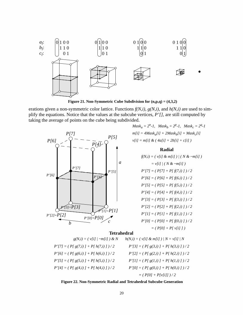
erations given a non-symmetric color lattice. Functions f(N,i), g(N,i), and h(N,i) are used to sim-plify the equations. Notice that the values at the subcube vertices, P’[], are still computed bytaking the average of points on the cube being subdivided.

0 1 0 0 1 1 0 0 1

al:bl:cl:

0 1 0 0 1 1 0 0 1

0 1 0 0 1 1 0 0 1

0 1 0 0 1 1 0 0 1

Figure 21. Non-Symmetric Cube Subdivision for (n,p,q) = (4,3,2)

Maska = 2n-1, Maskb = 2p-1, Maskc = 2q-1

m[i] = 4Maska[i] + 2Maskb[i] + Maskc[i]

v[i] = m[i] & ( 4a[i] + 2b[i] + c[i] )

Figure 22. Non-Symmetric Radial and Tetrahedral Subcube Generation

Tetrahedral

f(N,i) = ( v[i] & m[i] ) | ( N & ~m[i] )

= v[i] | ( N & ~m[i] )

P’[7] = ( P[7] + P[ f(7,i) ] ) / 2

P’[6] = ( P[6] + P[ f(6,i) ] ) / 2

P’[5] = ( P[5] + P[ f(5,i) ] ) / 2

P’[4] = ( P[4] + P[ f(4,i) ] ) / 2

P’[3] = ( P[3] + P[ f(3,i) ] ) / 2

P’[2] = ( P[2] + P[ f(2,i) ] ) / 2

P’[1] = ( P[1] + P[ f(1,i) ] ) / 2

P’[0] = ( P[0] + P[ f(0,i) ] ) / 2

= ( P[0] + P[ v[i] ] )

Radial

P’[7] = ( P[ g(7,i) ] + P[ h(7,i) ] ) / 2

P’[6] = ( P[ g(6,i) ] + P[ h(6,i) ] ) / 2

P’[5] = ( P[ g(5,i) ] + P[ h(5,i) ] ) / 2

P’[4] = ( P[ g(4,i) ] + P[ h(4,i) ] ) / 2

P’[3] = ( P[ g(3,i) ] + P[ h(3,i) ] ) / 2

P’[2] = ( P[ g(2,i) ] + P[ h(2,i) ] ) / 2

P’[1] = ( P[ g(1,i) ] + P[ h(1,i) ] ) / 2

P’[0] = ( P[ g(0,i) ] + P[ h(0,i) ] ) / 2

= ( P[0] + P[v[i]] ) / 2

P’[1]=P[1]

P’[0]=P[0]P’[2]=P[2]

P’[3]=P[3]

P[4]

P[5]P[6]

P[7]

P’[4]

P’[5]P’[6]

P’[7]

a

b c

g(N,i) = ( v[i] | ~m[i] ) & N h(N,i) = ( v[i] & m[i] ) | N = v[i] | N

21

Figure 23 and 24 present the Non-Symmetric Radial and Pruned Tetrahedral Interpolations. Note,a common implementation (Vondran [18]) can be used for both by multiplexing the indices of theinput values.

Given d input dimensions, D output dimensions and 2(n,p,q) values between coarse lattice points,the number of computations for Non-Symmetric Radial Interpolation is: Each v[i] and m[i]require d adds, and d-1 shifts. One additional bitwise AND operation masks v[i] using m[i].There are max(n,p,q) vertices v[i] and max(n,p,q) masks m[i] generated, resulting inmax(n,p,q)*((2d-1)+(2d-1)+1) = max(n,p,q)*(4d-1) operations. Each f(N,i) requires 3 bitwiselogic operations (one bitwise OR, one AND, and one NOT). It can be shown that the number off(N,i) references is

As shown in Figure 23, 2max(n,p,q)-1 additions are used. One additional add and shift is needed peroutput component to divide and round, totaling (2max(n,p,q)-1)+1+1 = 2max(n,p,q)+1. In Figure 23,2max(n,p,q) memory references are shown, however, a cap can be implemented on the number ofmemory accesses at the number of vertices of the cube (2d vertices are on the cube). Thus, theminimum of the two is used, i.e. min(2d, 2max(n,p,q)). With D output components the total number

Figure 23. Non-Symmetric Radial Interpolation

+

+

+

+

+

+

+

+

+

+

+

+

+

+

+

P[0]

P[ v[3] ]

P[ v[2] ]

P[ f( v[2], 3) ]

P[ v[1] ]

P[ f( v[1], 3) ]

P[ f( v[1], 2) ]

P[ f( f( v[1], 2), 3) ]

P[ v[0] ]

P[ f( v[0], 3) ]

P[ f( v[0], 2) ]

P[ f( f( v[0], 2), 3) ]

P[ f ( v[0], 1) ]

P[ f( f( v[0], 1), 3) ]

P[ f( f( v[0], 1), 2) ]

P[ f( f( f( v[0], 1), 2), 3) ]

P’’’’[0] = (x,y,z)

P’’’[0]

P’’’[ v[0] ]

P’’[0]

P’’[ v[1] ]

P’’[ v[0] ]

P’’[ f( v[0], 1) ]

P’[0]

P’[ v[2] ]

P’[ v[1] ]

P’[ f( v[1], 2) ]

P’[ v[0] ]

P’[ f( v[0], 2) ]

P’[ f( v[0], 1) ]

P’[ f( f( v[0], 1), 2) ]

Where v[i] = m[i] & ( 4a[i] + 2b[i] + c[i] )f(N,i) = v[i] | ( N & ~m[i] )

number f N i,( ) references 2max n p q, ,( ) 1–

1 2i–

–( )i 1=

max n p q, ,( ) 1–

∑=

22

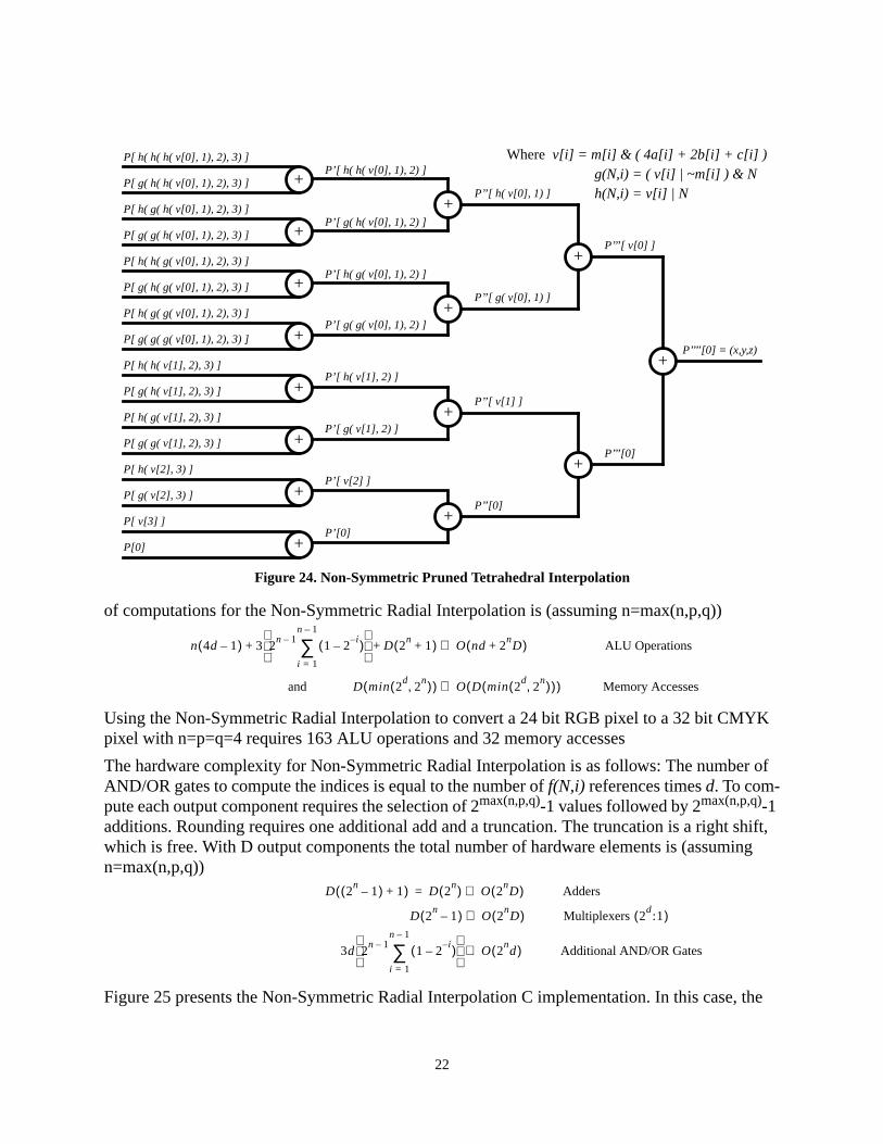
of computations for the Non-Symmetric Radial Interpolation is (assuming n=max(n,p,q))

Using the Non-Symmetric Radial Interpolation to convert a 24 bit RGB pixel to a 32 bit CMYKpixel with n=p=q=4 requires 163 ALU operations and 32 memory accesses

The hardware complexity for Non-Symmetric Radial Interpolation is as follows: The number ofAND/OR gates to compute the indices is equal to the number of f(N,i) references times d. To com-pute each output component requires the selection of 2max(n,p,q)-1 values followed by 2max(n,p,q)-1additions. Rounding requires one additional add and a truncation. The truncation is a right shift,which is free. With D output components the total number of hardware elements is (assumingn=max(n,p,q))

Figure 25 presents the Non-Symmetric Radial Interpolation C implementation. In this case, the

Figure 24. Non-Symmetric Pruned Tetrahedral Interpolation

+

+

+

+

+

+

+

+

+

+

+

+

+

+

+

P[0]

P[ v[3] ]

P[ g( v[2], 3) ]

P[ h( v[2], 3) ]

P[ g( g( v[1], 2), 3) ]

P[ h( g( v[1], 2), 3) ]

P[ g( h( v[1], 2), 3) ]

P[ h( h( v[1], 2), 3) ]

P[ g( g( g( v[0], 1), 2), 3) ]

P[ h( g( g( v[0], 1), 2), 3) ]

P[ g( h( g( v[0], 1), 2), 3) ]

P[ h( h( g( v[0], 1), 2), 3) ]

P[ g( g( h( v[0], 1), 2), 3) ]

P[ h( g( h( v[0], 1), 2), 3) ]

P[ g( h( h( v[0], 1), 2), 3) ]

P[ h( h( h( v[0], 1), 2), 3) ]

P’’’’[0] = (x,y,z)

P’’’[0]

P’’’[ v[0] ]

P’’[0]

P’’[ v[1] ]

P’’[ g( v[0], 1) ]

P’’[ h( v[0], 1) ]

P’[0]

P’[ v[2] ]

P’[ g( v[1], 2) ]

P’[ h( v[1], 2) ]

P’[ g( g( v[0], 1), 2) ]

P’[ h( g( v[0], 1), 2) ]

P’[ g( h( v[0], 1), 2) ]

P’[ h( h( v[0], 1), 2) ]Where v[i] = m[i] & ( 4a[i] + 2b[i] + c[i] )

g(N,i) = ( v[i] | ~m[i] ) & Nh(N,i) = v[i] | N

n 4d 1–( ) 3 2n 1–

1 2i–

–( )i 1=

n 1–

∑

D 2n


and D min 2d

2n,( )( ) O D min 2

d2


D 2n

1–( ) 1+( ) D 2n( ) O 2

nD( )⇒= Adders

D 2n


d:1( )

3d 2n 1–

1 2i–

–( )i 1=

n 1–

∑


23

input consists of arrays of input components, cube vertices (points), and lattice resolution values.The output is an array of components corresponding to the color in the output space. A cube ver-tex point array is passed in rather than a table pointer because the color lattice resolution for eachdimension may vary depending upon the region in the color space. How the color lattice is packedin the color table will determine the hashing scheme needed. Thus the presented implementationassumes the resolution and address into the color table have been computed prior to accessing theinterpolation routine. The remaining portion of Figure 24 follows closely the Non-SymmetricRadial Interpolation method previously derived.

Figure 25. Non-Symmetric Radial Interpolation C Implementation

#define f(v, m, N) ( v | ( N & ~m ) )/*************************************************//** nonsym_radial_interpolation() **//*************************************************/void nonsym_radial_interpolation( unsigned char input[], unsigned char point[][8], unsigned char resolution[], unsigned char output[] ){ register unsigned char Amask, Bmask, Cmask ; register int a, b, c, x, y, z ; register unsigned char m0, m1, m2, m3 ; register unsigned char v0, v1, v2, v3 ; register unsigned char f_v1_v0, f_v2_v1 ; register unsigned char f_v2_f_v1_v0, f_v2_v0 ; register unsigned char f_v3_v2, f_v3_f_v2_v1 ; register unsigned char f_v3_f_v2_f_v1_v0 ; register unsigned char f_v3_f_v2_v0, f_v3_v1 ; resister unsigned char f_v3_f_v1_v0, f_v3_v0 ;

/******************/ /* Generate Masks */ /******************/ Amask = ( 1 << resolution[0] ) - 1 ; Bmask = ( 1 << resolution[1] ) - 1 ; Cmask = ( 1 << resolution[2] ) - 1 ;

/***************************************/ /* Snap last value to last table value */ /***************************************/ a = ( input[0] == 0x0ff ) ? 0x100 : (int) input[0] ; b = ( input[1] == 0x0ff ) ? 0x100 : (int) input[1] ; c = ( input[2] == 0x0ff ) ? 0x100 : (int) input[2] ;

/*************************************************/ /* Compute slices across masks and input components */ /*************************************************/ m0 = ( (Amask & 0x01) << 2 ) + ( (Bmask & 0x01) << 1 ) + (Cmask & 0x01); m1 = ( (Amask & 0x02) << 1 ) + (Bmask & 0x02) + ( (Cmask & 0x02) >> 1 ); m2 = (Amask & 0x04)

+ ( (Bmask & 0x04) >> 1 ) + ( (Cmask & 0x04) >> 2 ); m3 = ( (Amask & 0x08) >> 1 )

+ ( (Bmask & 0x08) >> 2 ) + ( (Cmask & 0x08) >> 3 ); v0 = m0 & ( ( (a & 0x01) << 2 ) + ( (b & 0x01) << 1 ) + (c & 0x01) ); v1 = m1 & ( ( (a & 0x02) << 1 ) + (b & 0x02) + ( (c & 0x02) >> 1 ) ) ; v2 = m2 & ( (a & 0x04) + ( (b & 0x04) >> 1 ) + ( (c & 0x04) >> 2 ) ) ; v3 = m3 & ( ( (a & 0x08) >> 1 ) + ( (b & 0x08) >> 2 ) + ( (c & 0x08) >> 3 ) ) ;

/*******************************/ /* Compute offset from origin. */ /*******************************/ f_v1_v0 = f(v1,m1,v0) ; f_v2_v1 = f(v2,m2,v1) ; f_v2_f_v1_v0 = f(v2,m2,f_v1_v0) ; f_v2_v0 = f(v2,m2,v0) ; f_v3_v2 = f(v3,m3,v2) ; f_v3_f_v2_v1 = f(v3,m3,f_v2_v1) ; f_v3_f_v2_f_v1_v0 = f(v3,m3,f_v2_f_v1_v0) ; f_v3_f_v2_v0 = f(v3,m3,f_v2_v0) ; f_v3_v1 = f(v3,m3,v1) ; f_v3_f_v1_v0 = f(v3,m3,f_v1_v0) ; f_v3_v0 = f(v3,m3,v0) ;

/*************/ /* Compute x */ /*************/ x = ( ( point[0][f_v3_f_v2_f_v1_v0] + point[0][f_v2_f_v1_v0] + point[0][f_v3_f_v1_v0] + point[0][f_v1_v0] + point[0][f_v3_f_v2_v0] + point[0][f_v2_v0] + point[0][f_v3_v0] + point[0][v0] + point[0][f_v3_f_v2_v1] + point[0][f_v2_v1] + point[0][f_v3_v1] + point[0][v1] + point[0][f_v3_v2] + point[0][v2] + point[0][v3] + point[0][0] + 0x08 ) >> 4 ) ; /*Round*/ /*************/ /* Compute y */ /*************/ y = ( ( point[1][f_v3_f_v2_f_v1_v0] + point[1][f_v2_f_v1_v0] + point[1][f_v3_f_v1_v0] + point[1][f_v1_v0] + point[1][f_v3_f_v2_v0] + point[1][f_v2_v0] + point[1][f_v3_v0] + point[1][v0] + point[1][f_v3_f_v2_v1] + point[1][f_v2_v1] + point[1][f_v3_v1] + point[1][v1] + point[1][f_v3_v2] + point[1][v2] + point[1][v3] + point[1][0] + 0x08 ) >> 4 ) ; /*Round*/ /*************/ /* Compute z */ /*************/ z = ( ( point[2][f_v3_f_v2_f_v1_v0] + point[2][f_v2_f_v1_v0] + point[2][f_v3_f_v1_v0] + point[2][f_v1_v0] + point[2][f_v3_f_v2_v0] + point[2][f_v2_v0] + point[2][f_v3_v0] + point[2][v0] + point[2][f_v3_f_v2_v1] + point[2][f_v2_v1] + point[2][f_v3_v1] + point[2][v1] + point[2][f_v3_v2] + point[2][v2] + point[2][v3] + point[2][0] + 0x08 ) >> 4 ) ; /*Round*/ /**********************/ /* Write back results */ /**********************/ output[0] = (char) x ; output[1] = (char) y ; output[2] = (char) z ;}

24

Figure 26 presents the VHDL implementation of the Non-Symmetric Radial Interpolation. Note,the implementation closely follows that of the Pruned Tetrahedral Interpolation in Figure 18. Thedifferences consist of the addition of the MASKS process and the lines “P’[2*j] = P[j] ;” and“P’[2*i+1]=v[i]|(P[i] & ~m[i]) ;” in the VERTICES process. No changes are made in the MUXand SUM processes (with the exception of several comment statements)

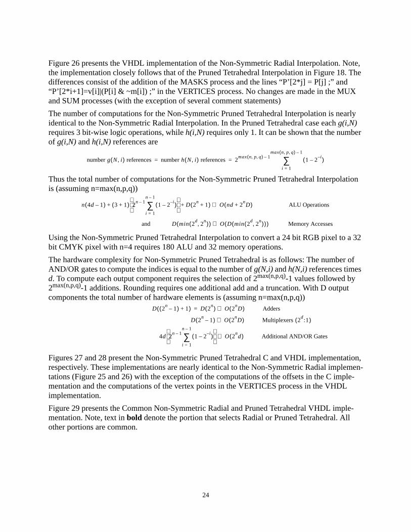
The number of computations for the Non-Symmetric Pruned Tetrahedral Interpolation is nearlyidentical to the Non-Symmetric Radial Interpolation. In the Pruned Tetrahedral case each g(i,N)requires 3 bit-wise logic operations, while h(i,N) requires only 1. It can be shown that the numberof g(i,N) and h(i,N) references are

Thus the total number of computations for the Non-Symmetric Pruned Tetrahedral Interpolationis (assuming n=max(n,p,q))

Using the Non-Symmetric Pruned Tetrahedral Interpolation to convert a 24 bit RGB pixel to a 32bit CMYK pixel with n=4 requires 180 ALU and 32 memory operations.

The hardware complexity for Non-Symmetric Pruned Tetrahedral is as follows: The number ofAND/OR gates to compute the indices is equal to the number of g(N,i) and h(N,i) references timesd. To compute each output component requires the selection of 2max(n,p,q)-1 values followed by2max(n,p,q)-1 additions. Rounding requires one additional add and a truncation. With D outputcomponents the total number of hardware elements is (assuming n=max(n,p,q))

Figures 27 and 28 present the Non-Symmetric Pruned Tetrahedral C and VHDL implementation,respectively. These implementations are nearly identical to the Non-Symmetric Radial implemen-tations (Figure 25 and 26) with the exception of the computations of the offsets in the C imple-mentation and the computations of the vertex points in the VERTICES process in the VHDLimplementation.

Figure 29 presents the Common Non-Symmetric Radial and Pruned Tetrahedral VHDL imple-mentation. Note, text in bold denote the portion that selects Radial or Pruned Tetrahedral. Allother portions are common.

number g N i,( ) references number h N i,( ) references 2max n p q, ,( ) 1–

1 2i–

–( )i 1=

max n p q, ,( ) 1–

∑= =

n 4d 1–( ) 3 1+( ) 2n 1–

1 2i–

–( )i 1=

n 1–

∑

D 2n


and D min 2d

2n,( )( ) O D min 2

d2


D 2n

1–( ) 1+( ) D 2n( ) O 2

nD( )⇒= Adders

D 2n


d:1( )

4d 2n 1–

1 2i–

–( )i 1=

n 1–

∑


25

Figure 26. Non-Symmetric Radial Interpolation VHDL Implementation

------------------------------------------ Non-Symmetric Radial Interpolation ------------------------------------------entity nonsym_radial isport ( -- Input Pixel -- input: in INPUT_ARRAY ; -- Vertex Points of Cube from Color Table -- point: in POINT_ARRAY ; -- Lattice Resolution -- resolution: in RESOLUTION_ARRAY ; -- Output Pixel -- output: out OUTPUT_ARRAY) ;end nonsym_radial ;

-----------------------------------------------------architecture nonsym_radialrtl of nonsym_radial is----------------------- -----------------------------

constant VERTEX_COUNT: INTEGER := 2**NUM_INTERP_BITS; signal mask: MASK_ARRAY ; signal vertex: VERTEX_ARRAY ; signal point_value: POINT_VALUE_ARRAY ;

begin

------------------------------------------------------- Compute Lattice Resolution Masks -------------------------------------------------------MASKS: process ( resolution ) variable top: INTEGER ;begin ------------------------ -- For each Component -- ------------------------ for i in 0 to 2 loop top := 0 ; ----------------------------------- -- Convert BIT_VECTOR to INTEGER -- ----------------------------------- for j in 2 downto 0 loop if ( resolution(i)(j) = ‘1’ ) then top := top + 2**j ; else top := top ; end if ; end loop ; ------------------- -- Generate Mask -- ------------------- for j in NUM_INTERP_BITS-1 downto 0 loop if ( j < top ) then mask(j)(i) <= ‘1’ ; else mask(j)(i) <= ‘0’ ; end if ; end loop ; end loop ;end process ;

------------------------------------------------------- Compute vertices. -------------------------------------------------------VERTICIES: process ( input, mask ) variable temp1, temp2: VERTEX_ARRAY ; variable limit: INTEGER ;begin ----------------------- -- Initialize Arrays -- ----------------------- temp2 := ( others => “000” ) ; ------------------------------------------------ -- For each slice across the interpolate bits -- ------------------------------------------------ for i in 0 to NUM_INTERP_BITS-1 loop ----------------------------------- -- limit is 0, 2, 6, 14, 30, ... -- ----------------------------------- limit := ( 2**(i+1) ) - 2 ; ------------------------------------ -- Load slice into limit location -- ------------------------------------ temp2(limit) := mask(i) and ( input(0)(i) & input(1)(i) & input(2)(i) ) ; temp1 := temp2 ; ----------------------------- -- for all values in temp1 -- ----------------------------- for j in (VERTEX_COUNT/2)-1 downto 0 loop if ( j < limit/2 ) then

-------------------- -- P’[2*j] = P[j] -- -------------------- temp2(2*j) := temp1(j) ; ---------------------------------- -- P’[2*j+1]=v[i]|(P[j] & ~m[i])-- ---------------------------------- temp2((2*j)+1) := temp1(limit)

or ( temp1(j) and not mask[i] ) ; else temp2 := temp2 ; end if ; end loop ; end loop ; --------------------------- -- Move into index array -- --------------------------- vertex <= temp2 ;end process ;

------------------------------------------------------- Select the values of vertices to be used by the ---- interpolation. The last two vertices are always ---- point(0) and the rounding constant. -------------------------------------------------------MUX: process ( vertex, point )begin for d in 0 to NUM_OUTPUT_DIMEN-1 loop point_value(d) <= (others => (others => ‘0’)); for i in 0 to VERTEX_COUNT-2 loop case vertex(i) is









------------------------------------------------------- Select the values of vertices to be used by the ---- interpolation. The last two vertices are always ---- point(0) and the rounding constant. -------------------------------------------------------SUM: process ( point_value ) variable temp: POINT_VALUES ; variable bound: INTEGER ;begin for d in 0 to NUM_OUTPUT_DIMEN-1 loop temp := point_value(d) ; bound := VERTEX_COUNT + 1 ; for i in 0 to NUM_INTERP_BITS loop for j in 0 to VERTEX_COUNT/2 loop if ( 2*j < bound ) then temp(j) := temp(2*j) ; else temp(j) := (others => ‘0’) ; end if ; if ( (2*j)+1 < bound ) then


------------------------------------------------end nonsym_radialrtl ;------------------------------------------------

26

Figure 27. Non-Symmetric Pruned Tetrahedral Interpolation C Implementation

#define g(v, m, N) ( ( v | ~m ) & N )#define h(v, N) ( v | N )/*************************************************//** nonsym_pruned_tetrahedral() **//*************************************************/void nonsym_pruned_tetrahedral( unsigned char input[], unsigned char point[][8], unsigned char resolution[], unsigned char output[] ){ register unsigned char Amask, Bmask, Cmask ; register int a, b, c, x, y, z ; register unsigned char m0, m1, m2, m3 ; register unsigned char v0, v1, v2, v3 ; register unsigned char g_v1_v0, h_v1_v0 ; register unsigned char g_v2_v1, g_v2_g_v1_v0 ; register unsigned char g_v2_h_v1_v0, h_v2_v1 ; register unsigned char h_v2_g_v1_v0, h_v2_h_v1_v0 ; register unsigned char g_v3_v2, g_v3_g_v2_v1 ; register unsigned char g_v3_h_v2_v1 ; register unsigned char g_v3_g_v2_g_v1_v0 ; register unsigned char g_v3_g_v2_h_v1_v0 ; register unsigned char g_v3_h_v2_g_v1_v0 ; register unsigned char g_v3_h_v2_h_v1_v0 ; register unsigned char h_v3_v2, h_v3_g_v2_v1 ; register unsigned char h_v3_h_v2_v1 ; register unsigned char h_v3_g_v2_g_v1_v0 ; register unsigned char h_v3_g_v2_h_v1_v0 ; register unsigned char h_v3_h_v2_g_v1_v0 ; register unsigned char h_v3_h_v2_h_v1_v0 ;

/******************/ /* Generate Masks */ /******************/ Amask = ( 1 << resolution[0] ) - 1 ; Bmask = ( 1 << resolution[1] ) - 1 ; Cmask = ( 1 << resolution[2] ) - 1 ;

/***************************************/ /* Snap last value to last table value */ /***************************************/ a = ( input[0] == 0x0ff ) ? 0x100 : (int) input[0] ; b = ( input[1] == 0x0ff ) ? 0x100 : (int) input[1] ; c = ( input[2] == 0x0ff ) ? 0x100 : (int) input[2] ;

/*************************************************/ /* Compute slices across masks and input components */ /*************************************************/ m0 = ( (Amask & 0x01) << 2 ) + ( (Bmask & 0x01) << 1 ) + (Cmask & 0x01); m1 = ( (Amask & 0x02) << 1 ) + (Bmask & 0x02) + ( (Cmask & 0x02) >> 1 ); m2 = (Amask & 0x04)

+ ( (Bmask & 0x04) >> 1 ) + ( (Cmask & 0x04) >> 2 ); m3 = ( (Amask & 0x08) >> 1 )

+ ( (Bmask & 0x08) >> 2 ) + ( (Cmask & 0x08) >> 3 ); v0 = m0 & ( ( (a & 0x01) << 2 ) + ( (b & 0x01) << 1 ) + (c & 0x01) ) ; v1 = m1 & ( ( (a & 0x02) << 1 ) + (b & 0x02) + ( (c & 0x02) >> 1 ) ) ; v2 = m2 & ( (a & 0x04) + ( (b & 0x04) >> 1 ) + ( (c & 0x04) >> 2 ) ) ; v3 = m3 & ( ( (a & 0x08) >> 1 ) + ( (b & 0x08) >> 2 ) + ( (c & 0x08) >> 3 ) ) ;

/*******************************/ /* Compute offset from origin. */ /*******************************/ g_v1_v0 = g(v1,m1,v0) ; h_v1_v0 = h(v1,v0) ; g_v2_v1 = g(v2,m2,v1) ; g_v2_g_v1_v0 = g(v2,m2,g_v1_v0) ; g_v2_h_v1_v0 = g(v2,m2,h_v1_v0) ; h_v2_v1 = h(v2,v1) ; h_v2_g_v1_v0 = h(v2,g_v1_v0) ; h_v2_h_v1_v0 = h(v2,h_v1_v0) ; g_v3_v2 = g(v3,m3,v2) ; g_v3_g_v2_v1 = g(v3,m3,g_v2_v1) ; g_v3_g_v2_g_v1_v0 = g(v3,m3,g_v2_g_v1_v0) ; g_v3_g_v2_h_v1_v0 = g(v3,m3,g_v2_h_v1_v0) ; g_v3_h_v2_v1 = g(v3,m3,h_v2_v1) ; g_v3_h_v2_g_v1_v0 = g(v3,m3,h_v2_g_v1_v0) ; g_v3_h_v2_h_v1_v0 = g(v3,m3,h_v2_h_v1_v0) ;

h_v3_v2 = h(v3,v2) ; h_v3_g_v2_v1 = h(v3,g_v2_v1) ; h_v3_g_v2_g_v1_v0 = h(v3,g_v2_g_v1_v0) ; h_v3_g_v2_h_v1_v0 = h(v3,g_v2_h_v1_v0) ; h_v3_h_v2_v1 = h(v3,h_v2_v1) ; h_v3_h_v2_g_v1_v0 = h(v3,h_v2_g_v1_v0) ; h_v3_h_v2_h_v1_v0 = h(v3,h_v2_h_v1_v0) ;

/*************/ /* Compute x */ /*************/ x = ( ( point[0][0] + point[0][v3] + point[0][g_v3_v2] + point[0][g_v3_g_v2_v1] + point[0][g_v3_g_v2_g_v1_v0] + point[0][g_v3_g_v2_h_v1_v0] + point[0][g_v3_h_v2_v1] + point[0][g_v3_h_v2_g_v1_v0] + point[0][g_v3_h_v2_h_v1_v0] + point[0][h_v3_v2] + point[0][h_v3_g_v2_v1] + point[0][h_v3_g_v2_g_v1_v0] + point[0][h_v3_g_v2_h_v1_v0] + point[0][h_v3_h_v2_v1] + point[0][h_v3_h_v2_g_v1_v0] + point[0][h_v3_h_v2_h_v1_v0] + 0x08 ) >> 4 ) ; /*Round*/

/*************/ /* Compute y */ /*************/ y = ( ( point[1][0] + point[1][v3] + point[1][g_v3_v2] + point[1][g_v3_g_v2_v1] + point[1][g_v3_g_v2_g_v1_v0] + point[1][g_v3_g_v2_h_v1_v0] + point[1][g_v3_h_v2_v1] + point[1][g_v3_h_v2_g_v1_v0] + point[1][g_v3_h_v2_h_v1_v0] + point[1][h_v3_v2] + point[1][h_v3_g_v2_v1] + point[1][h_v3_g_v2_g_v1_v0] + point[1][h_v3_g_v2_h_v1_v0] + point[1][h_v3_h_v2_v1] + point[1][h_v3_h_v2_g_v1_v0] + point[1][h_v3_h_v2_h_v1_v0] + 0x08 ) >> 4 ) ; /*Round*/

/*************/ /* Compute z */ /*************/ z = ( ( point[2][0] + point[2][v3] + point[2][g_v3_v2] + point[2][g_v3_g_v2_v1] + point[2][g_v3_g_v2_g_v1_v0] + point[2][g_v3_g_v2_h_v1_v0] + point[2][g_v3_h_v2_v1] + point[2][g_v3_h_v2_g_v1_v0] + point[2][g_v3_h_v2_h_v1_v0] + point[2][h_v3_v2] + point[2][h_v3_g_v2_v1] + point[2][h_v3_g_v2_g_v1_v0] + point[2][h_v3_g_v2_h_v1_v0] + point[2][h_v3_h_v2_v1] + point[2][h_v3_h_v2_g_v1_v0] + point[2][h_v3_h_v2_h_v1_v0] + 0x08 ) >> 4 ) ; /*Round*/

/**********************/ /* Write back results */ /**********************/ output[0] = (char) x ; output[1] = (char) y ; output[2] = (char) z ;

}

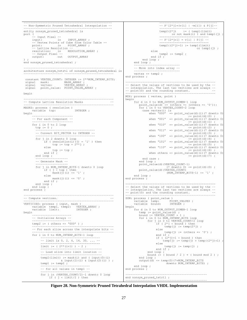
27

Figure 28. Non-Symmetric Pruned Tetrahedral Interpolation VHDL Implementation

------------------------------------------------------ Non-Symmetric Pruned Tetrahedral Interpolation ------------------------------------------------------entity nonsym_pruned_tetrahedral isport ( -- Input Pixel -- input: in INPUT_ARRAY ; -- Vertex Points of Cube from Color Table -- point: in POINT_ARRAY ; -- Lattice Resolution -- resolution: in RESOLUTION_ARRAY ; -- Output Pixel -- output: out OUTPUT_ARRAY) ;end nonsym_pruned_tetrahedral ;

-----------------------------------------------------architecture nonsym_tetrtl of nonsym_pruned_tetrahedral is----------------------- -----------------------------


begin

------------------------------------------------------- Compute Lattice Resolution Masks -------------------------------------------------------MASKS: process ( resolution ) variable top: INTEGER ;begin ------------------------ -- For each Component -- ------------------------ for i in 0 to 2 loop top := 0 ; ----------------------------------- -- Convert BIT_VECTOR to INTEGER -- ----------------------------------- for j in 2 downto 0 loop if ( resolution(i)(j) = ‘1’ ) then top := top + 2**j ; else top := top ; end if ; end loop ; ------------------- -- Generate Mask -- ------------------- for j in NUM_INTERP_BITS-1 downto 0 loop if ( j < top ) then mask(j)(i) <= ‘1’ ; else mask(j)(i) <= ‘0’ ; end if ; end loop ; end loop ;end process ;

------------------------------------------------------- Compute vertices. -------------------------------------------------------VERTICIES: process ( input, mask ) variable temp1, temp2: VERTEX_ARRAY ; variable limit: INTEGER ;begin ----------------------- -- Initialize Arrays -- ----------------------- temp2 := ( others => “000” ) ; ------------------------------------------------ -- For each slice across the interpolate bits -- ------------------------------------------------ for i in 0 to NUM_INTERP_BITS-1 loop ----------------------------------- -- limit is 0, 2, 6, 14, 30, ... -- ----------------------------------- limit := ( 2**(i+1) ) - 2 ; ------------------------------------ -- Load slice into limit location -- ------------------------------------ temp2(limit) := mask(i) and ( input(0)(i) & input(1)(i) & input(2)(i) ) ; temp1 := temp2 ; ----------------------------- -- for all values in temp1 -- ----------------------------- for j in (VERTEX_COUNT/2)-1 downto 0 loop if ( j < limit/2 ) then

---------------------------------- -- P’[2*j]=(v[i] | ~m[i]) & P[j]-- ---------------------------------- temp2(2*j) := ( temp1(limit)

or not mask(i) ) and temp1(j) ; ----------------------------- -- P’[2*j+1] = v[i] | P[j] -- ----------------------------- temp2((2*j)+1) := temp1(limit) or temp1(j) ; else temp2 := temp2 ; end if ; end loop ; end loop ; --------------------------- -- Move into index array -- --------------------------- vertex <= temp2 ;end process ;












------------------------------------------------end nonsym_pruned_tetrtl ;------------------------------------------------

28

Figure 29. Common Non-Symmetric Radial and Pruned Tetrahedral VHDL Implementation

------------------------------------------------------ Non-Symmetric Pruned Tetrahedral Interpolation ------------------------------------------------------entity nonsym_radial_tetr isport ( -- Interpolation Select -- tetra_not_radial: in STD_LOGIC ; -- Input Pixel -- input: in INPUT_ARRAY ; -- Vertex Points of Cube from Color Table -- point: in POINT_ARRAY ; -- Lattice Resolution -- resolution: in RESOLUTION_ARRAY ; -- Output Pixel -- output: out OUTPUT_ARRAY) ;end nonsym_pruned_tetrahedral ;

-----------------------------------------------------architecture nonsym_radial_tetrtl of nonsym_radial_tetr is----------------------- -----------------------------


begin

------------------------------------------------------- Compute Lattice Resolution Masks -------------------------------------------------------MASKS: process ( resolution ) variable top: INTEGER ;begin for i in 0 to 2 loop top := 0 ; for j in 2 downto 0 loop if ( resolution(i)(j) = ‘1’ ) then top := top + 2**j ; else top := top ; end if ; end loop ; for j in NUM_INTERP_BITS-1 downto 0 loop if ( j < top ) then mask(j)(i) <= ‘1’ ; else mask(j)(i) <= ‘0’ ; end if ; end loop ; end loop ;end process ;

------------------------------------------------------- Compute vertices. -------------------------------------------------------VERTICIES: process ( tetra_not_radial, input, mask ) variable temp1, temp2: VERTEX_ARRAY ; variable limit: INTEGER ;begin temp2 := ( others => “000” ) ; for i in 0 to NUM_INTERP_BITS-1 loop limit := ( 2**(i+1) ) - 2 ; temp2(limit) := mask(i) and ( input(0)(i) & input(1)(i) & input(2)(i) ) ; temp1 := temp2 ; for j in (VERTEX_COUNT/2)-1 downto 0 loop if ( j < limit/2 ) then --------------------------------- -- Select Radial or Tetrahedral-- --------------------------------- if ( tetra_not_radial = ‘0’ ) then ------------ -- Radial -- ------------ -------------------- -- P’[2*j] = P[j] -- -------------------- temp2(2*j) := temp1(j) ; ------------------------------ -- P’[2*j+1]=v[i]|(P[j]&~m[i]) ------------------------------ temp2((2*j)+1) := temp1(limit)

or (temp1(j) and not mask(i)); else

------------------------------ -- NonSym Pruned Tetrahedral - ------------------------------ ------------------------------ -- P’[2*j]=(v[i]|~m[i])&P[j]-- ------------------------------ temp2(2*j) := ( temp1(limit)

or not mask(i) ) and temp1(j) ; --------------------------- -- P’[2*j+1] = v[i]|P[j] -- --------------------------- temp2((2*j)+1) := temp1(limit) or temp1(j) ; end if ; else temp2 := temp2 ; end if ; end loop ; end loop ; vertex <= temp2 ;end process ;











temp(j) := temp(j) + temp((2*j)+1) ; else temp(j) := temp(j) ; end if ; end loop ; bound := ( bound / 2 ) + ( bound mod 2 ) ; end loop ; output(d) <= temp(0)(7+NUM_INTERP_BITS downto NUM_INTERP_BITS) ; end loop ;end process ;------------------------------------------------end nonsym_radial_tetrtl ;------------------------------------------------

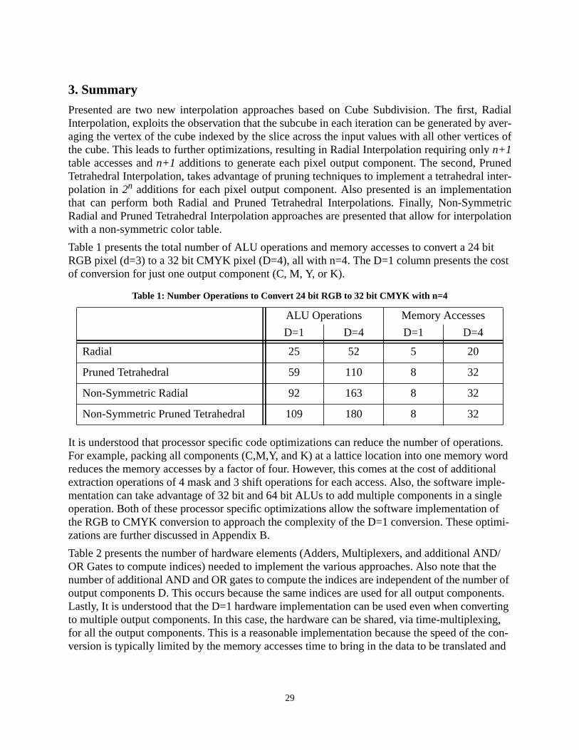
29

3. Summary

Presented are two new interpolation approaches based on Cube Subdivision. The first, RadialInterpolation, exploits the observation that the subcube in each iteration can be generated by aver-aging the vertex of the cube indexed by the slice across the input values with all other vertices ofthe cube. This leads to further optimizations, resulting in Radial Interpolation requiring only n+1table accesses and n+1 additions to generate each pixel output component. The second, PrunedTetrahedral Interpolation, takes advantage of pruning techniques to implement a tetrahedral inter-polation in 2n additions for each pixel output component. Also presented is an implementationthat can perform both Radial and Pruned Tetrahedral Interpolations. Finally, Non-SymmetricRadial and Pruned Tetrahedral Interpolation approaches are presented that allow for interpolationwith a non-symmetric color table.

Table 1 presents the total number of ALU operations and memory accesses to convert a 24 bitRGB pixel (d=3) to a 32 bit CMYK pixel (D=4), all with n=4. The D=1 column presents the costof conversion for just one output component (C, M, Y, or K).

It is understood that processor specific code optimizations can reduce the number of operations.For example, packing all components (C,M,Y, and K) at a lattice location into one memory wordreduces the memory accesses by a factor of four. However, this comes at the cost of additionalextraction operations of 4 mask and 3 shift operations for each access. Also, the software imple-mentation can take advantage of 32 bit and 64 bit ALUs to add multiple components in a singleoperation. Both of these processor specific optimizations allow the software implementation ofthe RGB to CMYK conversion to approach the complexity of the D=1 conversion. These optimi-zations are further discussed in Appendix B.

Table 2 presents the number of hardware elements (Adders, Multiplexers, and additional AND/OR Gates to compute indices) needed to implement the various approaches. Also note that thenumber of additional AND and OR gates to compute the indices are independent of the number ofoutput components D. This occurs because the same indices are used for all output components.Lastly, It is understood that the D=1 hardware implementation can be used even when convertingto multiple output components. In this case, the hardware can be shared, via time-multiplexing,for all the output components. This is a reasonable implementation because the speed of the con-version is typically limited by the memory accesses time to bring in the data to be translated and

Table 1: Number Operations to Convert 24 bit RGB to 32 bit CMYK with n=4

ALU Operations Memory Accesses

D=1 D=4 D=1 D=4

Radial 25 52 5 20

Pruned Tetrahedral 59 110 8 32

Non-Symmetric Radial 92 163 8 32

Non-Symmetric Pruned Tetrahedral 109 180 8 32

30

to write out the translated data. Thus, in current technologies, plenty of time exists to time-multi-plex the components through the conversion circuitry.

Appendix A. VHDL Package (Header) file

Figure 30 shows the VHDL package (header) file used for the VHDL implementations presented.

Appendix B. C Code Optimizations

By packing all the color components for a lattice point into the same word, the number of memoryreferences can be reduced. Figure 31 presents an alternative implementation to that presented inFigure 12. Notice that the number of memory operations is reduce to five accesses, which comesat the cost of additional mask and shift operations. This optimization can be applied to the otherpresented interpolations. Table 3 presents the number of operations and memory accesses for thevarious interpolation techniques with this optimization. It should be understood, the presents opti-mization does not apply to the hardware implementation.

Table 2: Number Hardware Elements to Convert 24 bit RGB to 32 bit CMYK with n=4

Adders Multiplexers AND/OR Gates

D=1 D=4 D=1 D=4 D=1 D=4

Radial 5 20 5 20 0 0

Pruned Tetrahedral 16 64 15 60 66 66

Non-Symmetric Radial 16 64 15 60 153 153

Non-Symmetric Pruned Tetrahedral 16 64 15 60 204 204

LIBRARY ieee ;USE ieee.std_logic_1164.all ;USE ieee.std_logic_arith.all;USE ieee.std_logic_unsigned.all;--------------------------------------------------

package interpolation_pkg is

constant NUM_INTERP_BITS: INTEGER := 4 ; constant NUM_OUTPUT_DIMEN: INTEGER := 4 ;

type INPUT_ARRAY is array (2 downto 0) of STD_LOGIC_VECTOR(NUM_INTERP_BITS-1 downto 0) ; type CUBE_POINTS is array (7 downto 0) of STD_LOGIC_VECTOR(7 downto 0) ; type POINT_ARRAY is array (NUM_OUTPUT_DIMEN-1 downto 0) of CUBE_POINTS ; type OUTPUT_ARRAY is array (NUM_OUTPUT_DIMEN-1 downto 0) of STD_LOGIC_VECTOR(7 downto 0) ; type VERTEX_ARRAY is array (NUM_INTERP_BITS-1 downto 0) of STD_LOGIC_VECTOR(2 downto 0) ; type POINT_VALUES is array (NUM_INTERP_BITS+1 downto 0) of STD_LOGIC_VECTOR(7+NUM_INTERP_BITS downto 0); type POINT_VALUE_ARRAY is array (NUM_OUTPUT_DIMEN-1 downto 0) of POINT_VALUES ; type RESOLUTION_ARRAY is array (2 downto 0) of STD_LOGIC_VECTOR(2 downto 0) ; type MASK_ARRAY is array (VERTEX_COUNT-2 downto 0) of STD_LOGIC_VECTOR(2 downto 0) ;

end interpolation_pkg ;------------------------------------------package body interpolation_pkg is------------------------------------------end interpolation_pkg ;

Figure 30. Package File for VHDL Implementations

31

Table 3: Number Operations to Convert 24 bit RGB to 32 bit CMYK with Optimizations

ALU Operations Memory Accesses

D=1 D=4 D=1 D=4

Radial 30 76 5 5

Pruned Tetrahedral 67 166 8 8

Non-Symmetric Radial 100 219 8 8

Non-Symmetric Pruned Tetrahedral 117 236 8 8

#define C_INC 1#define B_INC C_INC*17#define A_INC B_INC*17#define TABLE_INC A_INC*17/******************************************//** radial_interpolation() **//******************************************/void radial_interpolation(unsigned char input[],unsigned int table[TABLE_INC], unsigned char output[]){

register unsigned origin, p0, p1, p2, p3, p4 ;register int a, b, c ;register int w, x, y, z ;

/**************************************//* Snap max value to last table value *//**************************************/a = ( input[0] == 0x0ff ) ? 0x100 : (int) input[0] ;b = ( input[1] == 0x0ff ) ? 0x100 : (int) input[1] ;c = ( input[2] == 0x0ff ) ? 0x100 : (int) input[2] ;

/***************************************//* Compute Indexes into table *//***************************************/origin = A_INC*(a >> 4) + B_INC*(b >> 4) + (c >> 4) ;

p0 = table[ origin ] ;p1 = table[ origin + A_INC*( (a & 0x01) )

+ B_INC*( (b & 0x01) ) + (c & 0x01) ] ;

p2 = table[ origin + A_INC*( (a & 0x02) >> 1 ) + B_INC*( (b & 0x02) >> 1 ) + (c & 0x02) >> 1 ] ;



/*************//* Compute w *//*************/w = ( ( p0 >> 24 ) + ( p1 >> 24 ) + ( ( p2 & 0xff000000 ) >> 23 ) + ( ( p3 & 0xff000000 ) >> 22 ) + ( ( p4 & 0xff000000 ) >> 21 ) + 0x08 ) >> 4 ; /* Round */

/*************//* Compute x *//*************/x = ( ( ( p0 & 0x00ff0000 ) >> 16 ) + ( ( p1 & 0x00ff0000 ) >> 16 ) + ( ( p2 & 0x00ff0000 ) >> 15 ) + ( ( p3 & 0x00ff0000 ) >> 14 ) + ( ( p4 & 0x00ff0000 ) >> 13 ) + 0x08 ) >> 4 ; /* Round */

/*************//* Compute y *//*************/y = ( ( ( p0 & 0x0000ff00 ) >> 8 ) + ( ( p1 & 0x0000ff00 ) >> 8 ) + ( ( p2 & 0x0000ff00 ) >> 7 ) + ( ( p3 & 0x0000ff00 ) >> 6 ) + ( ( p4 & 0x0000ff00 ) >> 5 ) + 0x08 ) >> 4 ; /* Round */

/*************//* Compute z *//*************/z = ( ( p0 & 0x000000ff ) + ( p1 & 0x000000ff ) + ( ( p2 & 0x000000ff ) << 1 ) + ( ( p3 & 0x000000ff ) << 2 ) + ( ( p4 & 0x000000ff ) << 3 ) + 0x08 ) >> 4 ; /* Round */

output[0] = (char) w ;output[1] = (char) x ;output[2] = (char) y ;output[3] = (char) z ;

}

Figure 31. Radial Interpolation C Implementation with Processor Specific Optimizations

32

References[1] Clark, D., Strong, D., and White, T., Method of Color Conversion with Improved Interpolation, U.S. Patent

4477833, Oct. 1984, pp. 1-14.

[2] Gondek, J., Subdivision Based Colormap Interpolation, Invention Disclosure, 1994, pp. 1-16.

[3] Franklin, P., Interpolation Methods and Apparatus, U.S. Patent 4334240, July 1980, pp. 1-10.

[4] Ikegami, H., Method for Transforming Color Signal and Apparatus for Executing the Method, U.S. Patent5313314, May 1994, pp. 1-20.

[5] Imao, K. and Ohuchi, S., Interpolation Method and Color Correction Method Using Interpolation, U.S. Patent5311332, May 1994, pp. 1-20.

[6] Kanamori, K., Yamada, O., Motomura, H., Kurosawa, T., and Fumoto, T., Method and Apparatus for Color Con-version, U.S. Patent 5428465, pp. 1-18.

[7] Kanamori, K., Yamada, O., Motomura, H., Rika, H., Fumoto, T., and Kotera, H., Color Converting Apparatus forPerforming a Three-Dimensional Color Conversion of a Colored Picture in a Color Space with a Small Capacityof Memory, U.S. Patent 5504821, Apr. 1996, pp. 1-60.

[8] Kasson, J., Nin, S., Plouffe, W., and Hafner, J., Performing Color Space Conversions with Three-DimensionalLinear Interpolation, Journal of Electronic Imaging, 4(3), July 1995, pp. 226-250.

[9] Kasson, J., Plouffe, W., An Analysis of Selected Computer Interchange Color Spaces, ACM Transactions onGraphics, 11(4), Oct. 1992, pp. 373-405.

[10] Pugsley, P. Colour Correcting Image Reproducing Methods and Apparatus, U.S. Patent 3893166, July 1, 1975,pp. 1-12.

[11] Pugsley, P., Image Reproducing Methods and Apparatus, U.K. Patent 1369702, Oct. 1974.

[12] Sakamoto, T., Linear Interpolating Method and Color Conversion Apparatus Using This Method, U.S. Patent4511989, Apr. 1985, pp. 1-18.

[13] Sakamoto, T. and Itooka, A., Linear Interpolator for Color Correction, U.S. Patent 4275413, June 1981, pp. 1-16.

[14] Stone, M., Cowan, W., Beatty, J., Color Gamut Mapping and the Printing of Digital Color Images, ACM Trans-actions on Graphics, 7(4), Oct. 1988, pp. 249-292.

[15] Van de Capelle, J., Roose, K., Debaere, E., and Pletinckx, D., Method and a Device for Converting a Color Coor-dinate Set, U.S. Patent 5268754, Dec. 7, 1993, pp. 1-20.

[16] Vondran, G., Apparatus for Generating Interplator Input Data, U.S. Patent 5717507, Feb. 1998.

[17] Vondran, G., Apparatus for Routing Interpolator Input Data by Performing a Selective Two’s Complement Basedon Sets of Lower and Higher Order Bits of Input Data, U.S. Patent 5666437, Sept. 1997, pp. 1-20.

[18] Vondran, G., Common Non-Symmetric Pruned Radial and Non-Symmetric Pruned Tetrahedral InterpolationHardware Implementation, Patent Application Docket No. 10971846-1, pp. 1-61.

[19] Vondran, G., Common Pruned Radial and Pruned Tetrahedral Interpolation Hardware Implementation, PatentApplication Docket No. 10970157-1, pp. 1-60.

[20] Vondran, G., Non-Symmetric Radial and Non-Symmetric Pruned Radial Interpolation, Patent ApplicationDocket No. 10970158-1, pp. 1-62.

[21] Vondran, G., Non-Symmetric Tetrahedral and Non-Symmetric Pruned Tetrahedral Interpolation, Patent Applica-tion Docket No. 10970156-1, pp. 1-64.

[22] Vondran, G., Radial and Pruned Radial Interpolation, Patent Application Docket No. 10970159-1, pp. 1-65.

[23] Vondran, G., Tetrahedral and Pruned Tetrahedral Interpolation, Patent Application Docket No. 10970160-1, pp.1-67.

radial and pruned tetrahedral interpolation techniques · 3 a cube is returned from the color table...

Documents