radial flow

Solution to a radial diffusion model with polynomialdecaying flux at the boundary

Yarith del Angel, Mayra Nunez-Lopez and Jorge X. Velasco-Hernandez

Instituto Mexicano del PetroleoPrograma de Matematicas Aplicadas y Computacion

March 13, 2012

Yarith del Angel, Mayra Nunez-Lopez and Jorge X. Velasco-Hernandez (IMP) March 13, 2012 1 / 16

Introduction

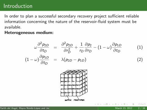
In order to plan a successful secondary recovery project sufficient reliableinformation concerning the nature of the reservoir-fluid system must beavailable.Heterogeneous medium:

ω∂2p2D

∂tD=

∂2p2D

∂r2D

+1

rD

∂p2

∂rD− (1− ω)

∂p1D

∂tD(1)

(1− ω)∂p1D

∂tD= λ(p2D − p1D) (2)

Figure: Heterogeneous porous moYarith del Angel, Mayra Nunez-Lopez and Jorge X. Velasco-Hernandez (IMP) March 13, 2012 2 / 16

Introduction

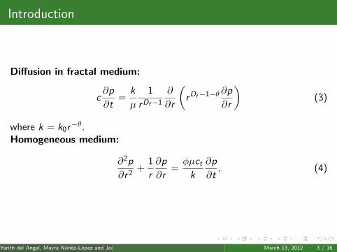
Diffusion in fractal medium:

c∂p

∂t=

k

µ

1

rDf−1

∂

∂r

(rDf−1−θ ∂p

∂r

)(3)

where k = k0r−θ.

Homogeneous medium:

∂2p

∂r2+

1

r

∂p

∂r=φµctk

∂p

∂t, (4)


Chicontepec

Chicontepec shows low production rates

Chicontepec is characterized not so much by a fractal network thatextends along particular formations, but rather by an extremecompartmentalization of clusters of the network.In Chicontepec, each cluster is embedded in a particular body ofsandstone which in itself is surrounded by very low permeabilitystructures.Whenever oil is extracted from a sandstone, it therefore depletes soondue to the relative limited volume that the sandstone body can hold.

Figure: pD vs tD for a closed boundary reservoir located at RD = 10.


The basic model

The observed behavior in the flow-rate production or in the pressure canbe attributed to many different factors other than fractures such as faults,stratification, and heterogeneities.Fluid flow:

∂2p

∂r2+

1

r

∂p

∂r=φµctk

∂p

∂t, (5)

rD =r

rw,

tD =kt

φµctr2w

,

pD = (pi − p)2πhk

qBµ,


The basic model

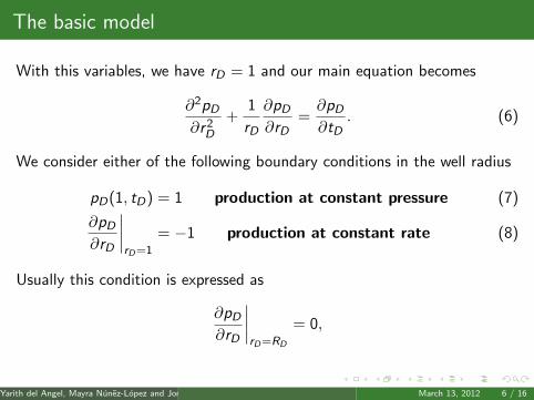
With this variables, we have rD = 1 and our main equation becomes

∂2pD∂r2

D

+1

rD

∂pD∂rD

=∂pD∂tD

. (6)

We consider either of the following boundary conditions in the well radius

pD(1, tD) = 1 production at constant pressure (7)

∂pD∂rD

∣∣∣∣rD=1

= −1 production at constant rate (8)

Usually this condition is expressed as

∂pD∂rD

∣∣∣∣rD=RD

= 0,


The basic model

Chicontepec:The oil depletes before the fluxes equilibrate albeit with the flux at theboundary being very small but non-zero.Boundary approximates the waiting times of a sub-diffusive flow outsidethe sandstone:

∂pD∂rD

∣∣∣∣rD=RD

= −ε(1− t−αD ), (9)

Finally, letpD(rD , 0) = 0. (10)


Closed reservoir

Dimensionless Time

Dim

ensi

onle

ss P

ress

ure

0 5 10 15 20 25 30

1.0

1.5

2.0

Figure: pD vs tD for a closed boundary reservoir located at RD = 10.

pD(1, tD) =2

R2 − 1tD +

R2D

R2D − 1

ln (RD)− 1

2

+2∞∑i=1

e−u2i tD

u2i

J21 (RDui )(

J21 (RDui )− J2

1 (ui )) . (11)


A model with variable flux at the boundary

Interior boundary condition(∂pD∂rD

)rD=1

= −1 , tD > 0 .

and exterior boundary condition(∂pD∂rD

)rD=RD

= H(tD − 1)ε(1− t−αD )

(∂pD∂rD

)rD=RD

=

{0, tD ≤ 1

ε(1− t−αD ), tD > 1(12)

pD(rD , s) =K1(RD

√s)I0(rD

√s) + I1(RD

√s)K0(rD

√s)

s32

[I1(RD

√s)K1(

√s)− I1(

√s)K1(RD

√s)] + f (s), (13)


A model with variable flux at the boundary

The production rate decreases very fast and the reservoir gradually fills

Dimensionless Time

Dim

ensi

onle

ss P

ress

ure

---- Ε=0

---- Ε=1.5

- - Ε=2.5

---- Ε=0.5

---- Ε=0.85

2000 4000 6000 8000 10 000

4.0

4.5

5.0

Figure: The influence of ε on the radial model with flux at the boundary can beseen in the curve pD vs tD and external radius RD = 200.


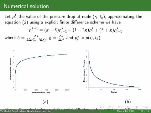
Numerical solution

Let pki the value of the pressure drop at node (ri , tk), approximating theequation (2) using a explicit finite difference scheme we have

pk+1i = (g − fi )p

ki−1 + (1− 2g)pki + (fi + g)pki+1

where fi = ∆t2∆r(1+i∆r) , g = ∆t

∆r2 and pki ≈ p(ri , tk),

0

1

2

3

4

5

6

0 2000 4000 6000 8000 10000

Dim

en

sio

nle

ss

Pre

ssu

re

Dimensionless Time

0

1

2

3

4

5

6

0 50 100 150 200

Dim

en

sio

nle

ss

Pre

ssu

re

Radius

(a) (b)

Figure: Numerical solution of the radial diffusion with parameters ε=0.3 andα=0.4. (a) Plot of pD vs tD at rD = 1. (b) Plot of pD vs rD at t = T .


Numerical solution

0

1

2

3

4

5

6

0 2000 4000 6000 8000 10000

Dim

en

sio

nle

ss P

ress

ure

Dimensionless Time

epsilon 0.1

epsilon 0.3

epsilon 0.8

epsilon 1

-1

0

1

2

3

4

5

6

0 50 100 150 200 250

Dim

en

sio

nle

ss P

ress

ure

Radius

epsilon 0.1

epsilon 0.3

epsilon 0.8

epsilon 1.0

(a) (b)

Figure: Numerical solution for different permeabilities for α=0.4.


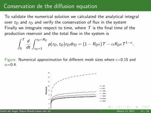
Conservation de the diffusion equation

To validate the numerical solution we calculated the analytical integralover tD and rD and verify the conservation of flux in the systemFinally we integrate respect to time, where T is the final time of theproduction reservoir and the total flow in the system is∫ T

0

d

dt

∫ rD=RD

rD=1p(rD , tD)rDdrD = (1− RDε)T − αRDεT

1−α.

Figure: Numerical approximation for different mesh sizes where ε=0.15 andα=0.4.

0

2

4

6

8

10

12

14

16

0 2000 4000 6000 8000 10000

Pressure

Time

100

500

1000

2000

4000

5000

6000


Conservation of the diffusion equation

We compare the numerical solution with different mesh size with thefollowing parameters: RD = 200, T = 10000, ε=0.15 and α=0.4, where∆t =0.0005.

Mesh size Numerical integral Relative error100 37609.10 3.43500 14450.80 0.701000 11512.00 0.352000 10038.60 0.184000 9300.90 0.095000 9153.27 0.076000 9054.84 0.067

Table: Relative errors with different mesh size with ∆t=0.0005.

Analytical integral: 8484.0928


Concluding remarks

We obtain a radial diffusion model for variable flux at the boundary torepresent the behavior of Chicontepec.Future work:

Obtain the analytical solution for different values of rD and comparewith the numerical solution

Calculate the semi-log derivative for long times to apply the model totest pressure .


References

[1] Van Everdingen, A.F., and Hurst W.: The Application of the LaplaceTransformation to Flow Problems in Reservoirs. Trans. AIME, Vol.186. (1949).

[2] Klins, M.A., Bouchard, A.J. and Cable, C.L.: A Polynomial Approachto the van Everdingen-Hurst Dimensionless Variables for WaterEncroachment. SPE, 15433. 320-326, (1988).

[3] Bourdarot: Well Testing: Interpretation Methods. ditions Technip,(1996).

[4] Carslaw H.S. and Jaeger J.C.: Operational Methods in AppliedMathematics. Dover, (1963).

[5] Morton K.W. and Mayers D.F.: Numerical solutions of PartialDifferential Equations. Cambridge, (1994).


radial flow

Documents