radiatia solara incidenta

int. j. geographical information science, 1997, vol. 11, no. 5, 475± 497

Research Article

Modelling topographic variation in solar radiation in a GIS

environment

LALIT KUMAR, ANDREW K. SKIDMORE andEDMUND KNOWLESSchool of Geography, University of New South Wales, Sydney, NSW 2052,Australiaemail: [email protected]

(Received 9 May 1996; accepted 5 December 1996 )

Abstract. Clear sky shortwave solar radiation varies in response to altitude andelevation, surface gradient (slope) and orientation (aspect) , as well as positionrelative to neighbouring surfaces. While the measurement of radiation ¯ ux on arelatively ¯ at surface is straightforward, it requires a dense network of stationsfor mountainous terrain. The model presented here uses a digital elevation modelto compute potential direct solar radiation and di� use radiation over a largearea, though the model may be modi® ed to include parameters such as cloudcover and precipitable water content of the atmosphere. The purpose of thisalgorithm is for applied work in forestry, ecology, biology and agriculture wherespatial variation of solar radiation is more important than calibrated values. Theability of the model to integrate radiation over long time periods in a computa-tionally inexpensive manner enables it to be used for modelling radiation per se,or input into other hydrological, climatological or biological models. The modelhas been implemented for commercially available GIS (viz. Arc Info and Genasys)and is available over the Internet.

1. Introduction

Solar radiation powers micrometeorological processes (such as soil heat ¯ ux andsoil temperature), sensible heat ¯ ux, surface and air temperatures, wind and turbulenttransport, evapotranspiration and growth and activity of plants and animals. In fact,99 8́ per cent of energy at the Earth’s surface comes from the Sun (Dickinson andCheremisino� 1980 ).

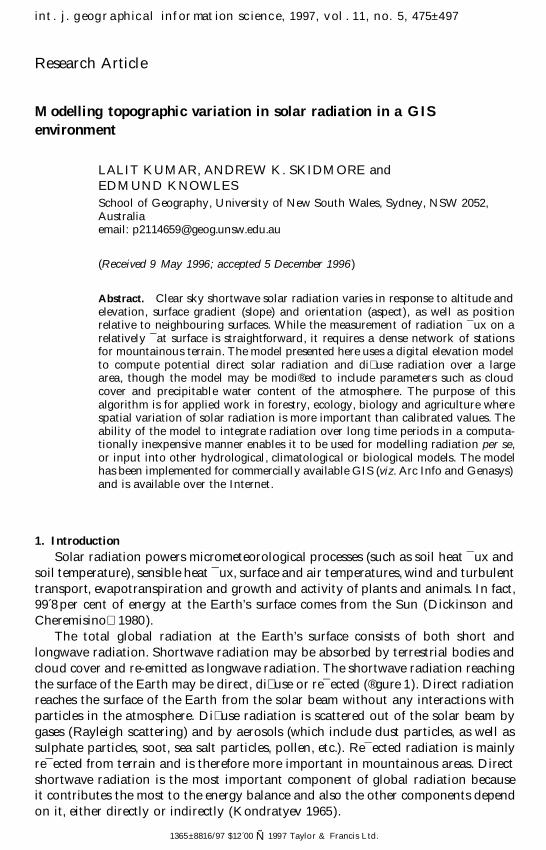
The total global radiation at the Earth’s surface consists of both short andlongwave radiation. Shortwave radiation may be absorbed by terrestrial bodies andcloud cover and re-emitted as longwave radiation. The shortwave radiation reachingthe surface of the Earth may be direct, di� use or re¯ ected ( ® gure 1). Direct radiationreaches the surface of the Earth from the solar beam without any interactions withparticles in the atmosphere. Di� use radiation is scattered out of the solar beam bygases (Rayleigh scattering) and by aerosols (which include dust particles, as well assulphate particles, soot, sea salt particles, pollen, etc.). Re¯ ected radiation is mainlyre¯ ected from terrain and is therefore more important in mountainous areas. Directshortwave radiation is the most important component of global radiation becauseit contributes the most to the energy balance and also the other components dependon it, either directly or indirectly (Kondratyev 1965).

1365 ± 8816/97 $12 0́0 Ñ 1997 Taylor & Francis Ltd.

L . Kumar et al.476

Figure 1. Downward irradiance received in a mountainous region: (1 ) direct irradiance,(2) di� use irradiance from the sky, and (3 ) terrain re¯ ected irradiance.

Global radiation at a location is roughly proportional to direct solar radiation,and varies with the geometry of the receiving surface. The other components, suchas di� use radiation, vary only slightly from slope to slope within a small area andthe variations can be linked to slope gradient (Kondratyev 1965, Williams et al.1972). In fact, di� use radiation comprises less than 16 per cent of total irradiance atvisible wavelengths in the green and red region (Dubayah 1992), rising to 30 percent for blue. The ¯ ux of clear-sky di� use radiation varies with slope orientationmuch the same way as the ¯ ux of direct solar radiation, hence preserving the spatialvariability in total radiation (Dubayah et al. 1989).

Parameters such as rainfall and temperature are frequently measured at one siteand generalized for the surrounding region but extrapolating vertical atmosphericvalues, even using satellites, is di� cult. Recording solar radiation at one site andextrapolating is seldom feasible as it is highly variable from place to place due tochanging slope (surface gradient) and aspect (surface orientation). On ¯ at terrainand under clear-sky conditions, the downwelling shortwave radiation is nearly thesame from point to point over relatively large areas and so one measurement canbe taken to be representative of the entire area. However for mountainous terrainsuch point measurements do not adequately represent the shortwave radiation overlarge areas because mountain terrain sets up localized weather conditions (Barry1981) and so point samples are representative of only the locality from which theyare collected. It is thus obvious that to get a reasonable accuracy in the measurementof incoming ¯ uxes in mountainous terrain one has to use either a very dense networkof data collection stations or use approaches such as radiation modelling (Duguay1993).

Solar radiation over large areas has often been estimated by measuring thenumber of hours of sunshine at a single site and then converting the hours intoradiation values by the use of empirical relationships, such as the AÊ ngstrom equation(AÊ ngstrom 1924, Glover and McCulloch 1958), and generalizing this for the wholearea. The conventional AÊ ngstrom equation is of the form

Q/QA=a+b n/N (1 )

Solar radiation modelling 477

where Q=total solar radiation on a horizontal surface on the EarthQA=radiation on a horizontal surface at the upper limit of the atmospheren=hours of bright sunshineN=total possible hours of sunshine, anda and b are constants found using regression.

Bu� o et al. (1972), Frank and Lee (1966) and Kondratyev (1969 ) have developedempirical relations between the e� ects of slope exposure (e.g., gradient and aspect(Skidmore 1990)) and clear sky radiation, but most of the results are in graphicalor tabular form. This may be good for engineers, who require only point speci® cdata, but in forestry and ecological studies the variation in solar radiation over astudy area is required. Swift (1976) modelled total shortwave radiation over a largearea but it required measurements of solar radiation on a nearby site in addition toslope and aspect information. The shading e� ects by adjacent features had to bevisually estimated and manually calculated. Nunez (1980) developed a model whichused cloud temperature data to obtain radiation ¯ uxes. Recently, Dubayah and Rich(1995) review the issues in modelling solar radiation for GIS.

Di� use sky irradiance under cloud free conditions may be estimated by assumingan isotropic sky, and calculating the proportion of the sky seen from a point (thatis using the equivalent of the viewshed operation in GIS) (Dubayah and Rich 1995).Under cloudy or partly cloudy conditions, di� use radiation is anisotropic which maybe explicitly modelled, but in practice this is computationally expensive to achieveas the di� use radiation from di� erent portions of the sky must be calculated. Moreimportantly, in order to calculate actual solar ¯ ux, ® eld data such as pyranometerdata (which measures actual incoming solar ¯ ux at a station), atmospheric opticaldata, or atmospheric pro® ling (sounding) must be used.

The aim of this research was to compute potential solar radiation (the amountof shortwave radiation received under clear-sky conditions), over a large area usingonly digital elevation and latitude data and to study the variation in radiation atdi� erent aspects and slopes. The model must cope with ¯ at or mountainous terrain,as well as shading by adjacent features. While the model calculates only the potentialbeam solar radiation and a simpli® ed di� use radiation, it can be modi® ed to includeother parameters such as e� ects of cloud cover and precipitable water content of theatmosphere, if such data are available. It should be noted that for many parts of theearth, these data are not readily available, so we wished to develop a pragmaticapproach to radiation modelling which may be utilized by GIS analysts. Thus theemphasis is on describing relative spatial variation in solar radiation, with modelledvalues as close to actual values as possible, rather than in exact values for validationand calibration purposes; relative solar radiation may be linked to the distributionof ¯ ora and fauna in the landscape, as well as productivity.

Any model which is established in a given site using as input data records ofclassical weather parameters produced either by individual site installation or by anearby meteorological station will only be applicable to that site. Therefore, whilegenerating the model, an attempt has been made to include widely accepted empiricalrelations at the expense of probably more rigorous computational methods whichrequire a lot of site speci® c data. As has been mentioned previously, site speci® cdata for mountainous terrain is rarely available, hence inclusion of such parametersin the model would probably render it unusable for a lot of areas where it is actuallymeant to be used. However, where general empirical relations have been used otherparameterizations are given and the reader is directed to relevant literature so that,where site speci® c data is available, these relations could be utilized.

L . Kumar et al.478

2. Method

2.1. Computational proceduresThe intensity of solar radiation is a function of the solar direction relative to the

local plane of the Earth’s surface at that instance. Variables such as solar azimuthangle and solar altitude angle change continuously throughout the day, and so haveto be calculated every time the intensity of solar radiation is computed. Solardeclination may be assumed to be constant and is calculated only once per day. Tosimplify the explanations, the Ptolemaic view of the Sun’s motion around the Earthwill be used; in other words the site is ® xed and is the centre of origin. Thefundamental equations used below are available from standard textbooks on solarengineering, such as Kreith and Kreider (1978), Du� e and Beckman (1991) andSayigh (1977 ).

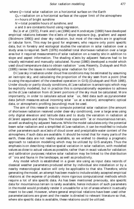
The Sun’s position in the sky is described by the solar altitude and solar azimuthangles. The solar altitude angle (a) is the angular elevation of the Sun above thehorizon ( ® gure 2). It is measured from the local horizontal plane upward to thecentre of the sun. The solar altitude angle changes continuously; that is daily andseasonally. It is zero at sunrise each day, increases as the Sun rises and reaches amaximum at solar noon and then decreases again until it reaches zero at sunset.The noon solar altitude angle varies seasonally; the seasonal change being due tothe declination angle changing daily.

The solar azimuth angle (as ) is measured in a horizontal plane between a duesouth line and the direction from the site to the sun as projected onto a horizontalplane ( ® gure 2). The solar altitude angle (a) and solar azimuth angle (as ) are relatedto the fundamental angles of latitude, solar declination (ds ) and hour angle (hs ) byequations (2 ) and (3) where L is the latitude of the site (Kreith and Kreider 1978).

sin a=sin L sin ds+cos L cos ds cos hs (2 )

sin as=cos ds sin hs/cos a (3 )

The hour angle describes how far east or west the Sun is from the local meridian.It is zero when the Sun is on the meridian and decreases at a rate of 15 ß per hour.By convention morning values are positive and afternoon values are negative.

Solar declination is the angle between the direction to the Sun and the plane ofthe Earth’s equator and is given in equation (4) (Du� e and Beckman 1991).

ds=23 4́5 sin (360ß (284+N )/365) (4)

Figure 2. Illustration of solar altitude and solar azimuth angles.


where N is the day number, 1 January being day 1 and 31 December being day 365.The declination varies from 23 4́5ß S to 23 4́5ß N. Again by convention values northof the equator are taken to be positive and those to the south are negative.

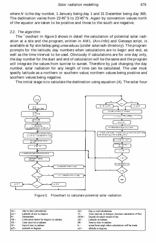
2.2. T he algorithmThe ¯ owchart in ® gure 3 shows in detail the calculation of potential solar radi-

ation at a site and the program, written in AML (Arc-Info) and Genasys script, isavailable at ftp site fatboy.geog.unsw.edu.au (under solarradn directory). The programprompts for the latitude, day numbers when calculations are to begin and end, aswell as the time interval to be used. Obviously if calculations are for one day only,the day number for the start and end of calculation will be the same and the programwill integrate the values from sunrise to sunset. Therefore by just changing the daynumber, solar radiation for any length of time can be calculated. The user mustspecify latitude as a northern or southern value; northern values being positive andsouthern values being negative.

The initial stage is to calculate the declination using equation (4). The solar hour

Figure 3. Flowchart to calculate potential solar radiation.

L . Kumar et al.480

angles at sunrise (hsr) and sunset (hss) for the day are also calculated. Sunrise is whensolar altitude angle is zero degrees, (equations (5) and (6)).

sin a=0=sin L sin ds+cos L cos ds cos hsr(a=0) (5)

[hsr=cos Õ 1 (Õ tan L tan ds ) (6 )

and hss=Õ hsr

Sunrise and sunset are the time when the centre of the sun is at the horizon, i.e.,solar altitude angle is taken from the centre of the Sun. Fleming et al. (1995) havesuggested the use of Õ 0 8́333ß as the altitude angle for calculating the sunrise timeas this takes atmospheric refraction into account. At this angle the top of the solardisc is just visible above the horizon and so starts illuminating the site, albeit withvery weak rays.

Once the sunrise and sunset times are calculated, solar radiation is integratedfrom sunrise to sunset. At this point it is necessary to decide on the time intervalbetween solar irradiance calculations. This decision depends on both the accuracyrequired as well as the terrain, and must be balanced against computational expense.A rugged terrain will cause increased shading e� ects as the Sun moves across thesky and so a smaller time interval should be used. For the example below, averagesolar radiation was calculated at the midpoint of a 30 minute interval; the midpointbeing taken to represent the average of the ¯ ux over the time interval.

The solar altitude and azimuth angles at the above hour angle are then calculatedusing equations (2) and (3). However, in using equation (3) to ® nd the azimuthangle, it is important to distinguish the case where the Sun is in the northern halfof the sky from the case where it is in the southern half. If cos hs is greater ( less)than tan ds /tan L then the Sun is in the northern (southern) half of the sky and itsazimuth angle is in the range Õ 90 ß to 90 ß (90 ß to 270ß ) .

In the next stage, shaded and illuminated points are calculated. The HILLSHADEcommand (in both Arc/Info and Genasys) creates a shaded relief grid by consideringthe illumination angle and shadows from a grid of elevation, solar azimuth angleand solar altitude angle. Shadows are de® ned by the local horizon at each cell. InArc/Info shadows are assigned a value of zero and illuminated cells are given a valueof one, while in Genasys the values obtained have to be reclassi® ed to get the shadedand illuminated cells.

Solar radiation received at a site will depend upon the solar ¯ ux outside theatmosphere, the optical air mass, water vapour and aerosol content of the atmos-phere. The solar ¯ ux (Io ) outside the atmosphere is given by Kreith and Kreider(1978) and Du� e and Beckman (1991) (equation (7)).

Io=So (1+0 0́344 cos(360ß N/365)) (W m Õ 2 ) (7 )

Equation (7) accounts for variation in the solar irradiance at the top of theatmosphere throughout the year as a result of the elliptical nature of the Earth’spath around the Sun. So , the solar constant, is the irradiance of an area perpendicularto the Sun’s rays just outside the atmosphere and at the mean Sun± Earth distance.The exact value of the solar constant is subject to much ongoing debate. A value of1353 W m Õ 2 has been accepted by NASA as a standard (Jansen 1985) and theSmithsonian Institute also uses this value; however recent publications have citedvalues of 1367 W m Õ 2 (Duncan et al. 1982, Wehrli 1985 ) and 1373 W m Õ 2 (Monteithand Unsworth 1990). The World Radiation Centre (WRC) has adopted a value of


1367 W m Õ 2 (Du� e and Beckman 1991) and so this is the value used for calculationsin this model.

2.2.1. Direct radiationSolar radiation is attenuated as it passes through the atmosphere and, in a

simpli® ed case, may be estimated using Bouger’s Law (Kreith and Kreider 1978;equation (8))

Ib=Io e ÕkM (8 )

where it is assumed that the sky is clear, Ib and Io are the terrestrial and extraterrestrialintensities of beam radiation, k is an absorption constant and M is the air massratio. The air mass ratio is the relative mass of air through which solar radiationmust pass to reach the surface of the Earth. It is the ratio of actual path length massto the mass when the Sun is directly overhead. It varies from M=1 when the Sunis overhead to about 30 when the Sun is at the horizon. The two main factorsa� ecting the air mass ratio are the direction of the path and the local altitude. Thepaths direction is described in terms of its zenith angle, y , which is the angle betweenthe path and the zenith position directly overhead. The ratio M is proportional tosec y , which is equal to 1/cos y (Gates 1980).

The adjustment in air mass for local altitude is made in terms of the localatmospheric pressure, p, and is de® ned in equation (9) where p is the local pressureand Mo and po are the corresponding air mass and pressure at sea level.

M= ( p/po ) Mo (9 )

This above formula is valid only for zenith angles less than 70 ß (Kreith andKreider 1978). When the zenith angle is greater than 70 ß , the secant approximationunderestimates solar energy because atmospheric refraction and the curvature of theEarth have not been accounted for. Frouin et al. (1989 ) have suggested the use ofequation (10).

M=[cos y+0 1́5 (93 8́85 Õ y) Õ 1 2́53 ] Õ 1 (10)

Keith and Kreider (1978) and Cartwright (1993) have suggested using the rela-tionship in equation (11). The model presented here used equation (11) to calculatethe value of air mass ratio.

M=[1229+ (614 sin a)2]1/2 Õ 614 sin a (11)

As the solar radiation passes through the Earth’s atmosphere it is modi® ed due to:

Ð absorption by di� erent gases in the atmosphere,Ð molecular (or Rayleigh) scattering by the permanent gases,Ð aerosol (Mie) scattering due to particulates.

Absorption by atmospheric molecules is a selective process that converts incomingenergy to heat, and is mainly due to water, oxygen, ozone and carbon dioxide.Equations describing the absorption e� ects of the above are given by Turner andSpencer (1972 ). A number of other gases absorb radiation but their e� ects arerelatively minor and for most practical purposes can be neglected (Forster 1984 ).

Atmospheric scattering can be either due to molecules of atmospheric gases ordue to smoke, haze and fumes (Richards 1993). Molecular scattering is consideredto have a dependence inversely proportional to the fourth power of the wavelength

L . Kumar et al.482

of radiation, i.e., l Õ 4 . Thus the molecular scattering at 0 5́ mm (visible blue) will be16 times greater than at 1 0́ mm (near-infrared ). As the primary constituents of theatmosphere and the thickness of the atmosphere remain essentially constant underclear sky conditions, molecular scattering can be considered constant for a particularwavelength. Aerosol scattering, on the other hand, is not constant and depends onthe size and vertical distribution of particulates. It has been suggested (Monteithand Unsworth 1990) that a l Õ 1´3 dependence can be used for continental regions.In an ideal clear atmosphere Rayleigh scattering is the only mechanism present(Richards 1993) and it accounts for the blueness of the sky.

The e� ects of the atmosphere in absorbing and scattering solar radiation arevariable with time as atmospheric conditions and the air mass ratio change.Atmospheric transmittance (t) values vary with location and elevation and rangebetween 0 and 1. According to Gates (1980) at very high elevations with extremelyclear air t may be as high as 0 8́, while for a clear sky with high turbidity it may beas low as 0 4́.

Hottel (1976) has presented a set of empirical equations for estimating beamradiation transmitted through clear atmosphere. The equations take into accountthe zenith angle as well as the altitude, and are stated in equation (12);

tb=a0+a1 e Õk/cos

y (12)

where tb is the atmospheric transmittance for beam radiation. a0 , a1 and k areconstants and for the standard atmosphere with 23 km visibility and altitudes lessthan 2 5́ km are given in equation (13).

a0=0 4́237Õ 0 0́0821 (6 Õ A)2

a1=0 5́055+0 0́0595 (6 5́ Õ A )2

k=0 2́711+0 0́1858 (2 5́ Õ A )2 (13)

where A is the altitude of the site in kilometres. Equations for a standard atmospherewith 5 km visibility are also given by Hottel.

Kreith and Kreider (1978 ) have described the atmospheric transmittance forbeam radiation by the empirical relationship given in equation (14).

tb=0 5́6 (e Õ 0 6́5 M+e Õ 0 0́95 M) (14)

The constants account for attenuation of radiation by the di� erent factors discussedabove. Because scattering is wavelength dependent, the coe� cients represent anaverage scattering over all wavelengths. This relationship gives the atmospherictransmittance for clear skies to within 3 per cent accuracy (Kreith and Kreider 1978)and the relationship has also been used by Cartwright (1993 ). Equation (14) is usedin the model instead of the Bouger form (equation (8)) as the Bouger form appliesto a simpli® ed case and does not account for factors considered in developingequations (14) and (15).

Therefore the shortwave solar radiation striking a surface normal to the Sun’srays (Is ) is given by equation (15). The atmospheric transmittance in the aboveequation can be replaced by site speci® c values if they are available.

Is=Io tb (15)

The last stage is to calculate the solar radiation on a tilted surface (Ip ) . This isgiven in equation (16), where cos i=sin ds (sin L cos b Õ cos L sin b cos aw )+


cos ds cos hs (cos L cos b+sin L sin b cos aw )+cos ds sin b sin aw sin hs . i is the anglebetween the normal to the surface and the direction to the Sun and b is the tilt angleof the surface (slope) and aw is the azimuth angle of the surface (aspect). Slope andaspect of each grid cell are stored in separate grids, and accessed as required tocalculate the solar radiation.

Ip=Is cos i (16)

2.2.2. Di� use and re¯ ected insolationDi� use solar radiation (Id ) was calculated using the method suggested by Gates

(1980), and is given by the equation (17).

Id=Io td cos2 b/2 sin a (17)

where td is the radiation di� usion coe� cient. td can be related to tb by equation(18) (Liu and Jordan 1960) which applies to clear sky conditions, and shows thatthe greater the direct solar beam transmittance, the smaller the transmittance toscattered skylight. Typical values of direct beam transmittance for a dust free, clearsky range from 0 4́00 to 0 8́00, and the corresponding di� use skylight transmissionvaries from 0 1́53 to 0 0́37 (Gates 1980).

td=0 2́71 Õ 0 2́94 tb (18)

The magnitude of re¯ ected radiation depends on the slope of the surface and theground re¯ ectance coe� cient. The re¯ ected radiation here is the ground-re¯ ectedradiation, both direct sunlight and di� use skylight, impinging on the slope afterbeing re¯ ected from other surfaces visible above the slope’s local horizon. There¯ ecting surfaces are considered to be Lambertian. Here re¯ ected radiation (Ir ) wascalculated based on equation (19) (Gates 1980)

Ir= rI0 tr sin2 b/2 sin a (19)

where r is the ground re¯ ectance coe� cient and tr is the re¯ ectance transmittivity.The ground re¯ ectance coe� cient is the mean re¯ ectivity of the surface over a speci® cspectral band normalized by the full solar spectrum (Monteith and Unsworth 1990 ).tr can be related to tb by the relationship in equation (20) (Gates 1980).

tr=0 2́71+0 7́06 tb (20)

A value of 0 2́0 was used for the re¯ ectance coe� cient of vegetation (Gates 1980).

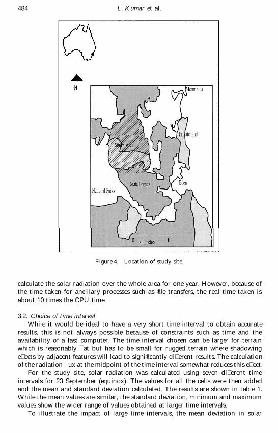
2.3. Study siteThe algorithm described was used to compute the potential shortwave radiation

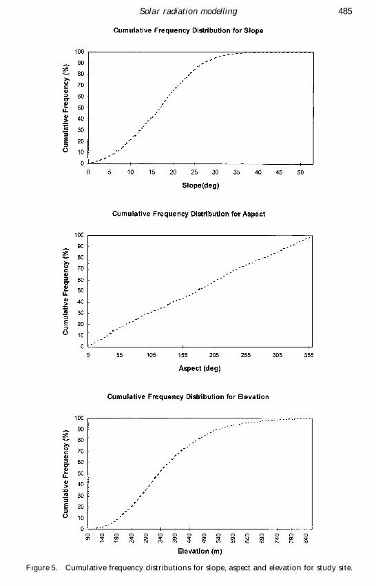
at Nullica State Forest near Eden, New South Wales, at a latitude of 36 5́ ß S. Theterrain at the site is fairly rugged with elevation ranging from 9 to 880 metres.Figure 4 shows the location of the site while ® gure 5 gives a summary of the slope,aspect and elevation distributions. The total area of the study site was 16406 ha,made up of 182288 30 m by 30 m grid cells.

3. Results and discussion

3.1. Computation timeThe program was run on a Sun Sparc5 workstation. For each time interval it

took about 2 3́5 seconds of CPU time to compute the solar radiation for the 182288grid cells. Using a time interval of 30 minutes it takes 5 7́ hours of CPU time to

L . Kumar et al.484

Figure 4. Location of study site.

calculate the solar radiation over the whole area for one year. However, because ofthe time taken for ancillary processes such as ® le transfers, the real time taken isabout 10 times the CPU time.

3.2. Choice of time intervalWhile it would be ideal to have a very short time interval to obtain accurate

results, this is not always possible because of constraints such as time and theavailability of a fast computer. The time interval chosen can be larger for terrainwhich is reasonably ¯ at but has to be small for rugged terrain where shadowinge� ects by adjacent features will lead to signi® cantly di� erent results. The calculationof the radiation ¯ ux at the midpoint of the time interval somewhat reduces this e� ect.

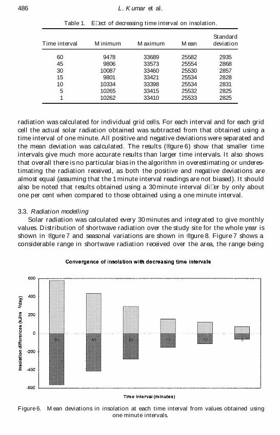
For the study site, solar radiation was calculated using seven di� erent timeintervals for 23 September (equinox). The values for all the cells were then addedand the mean and standard deviation calculated. The results are shown in table 1.While the mean values are similar, the standard deviation, minimum and maximumvalues show the wider range of values obtained at larger time intervals.

To illustrate the impact of large time intervals, the mean deviation in solar


Figure 5. Cumulative frequency distributions for slope, aspect and elevation for study site.

L . Kumar et al.486

Table 1. E� ect of decreasing time interval on insolation.

StandardTime interval Minimum Maximum Mean deviation

60 9478 33689 25582 293545 9806 33573 25554 286830 10087 33460 25530 285715 9801 33421 25534 282810 10334 33398 25534 28315 10265 33415 25532 28251 10262 33410 25533 2825

radiation was calculated for individual grid cells. For each interval and for each gridcell the actual solar radiation obtained was subtracted from that obtained using atime interval of one minute. All positive and negative deviations were separated andthe mean deviation was calculated. The results ( ® gure 6) show that smaller timeintervals give much more accurate results than larger time intervals. It also showsthat overall there is no particular bias in the algorithm in overestimating or underes-timating the radiation received, as both the positive and negative deviations arealmost equal (assuming that the 1 minute interval readings are not biased). It shouldalso be noted that results obtained using a 30 minute interval di� er by only aboutone per cent when compared to those obtained using a one minute interval.

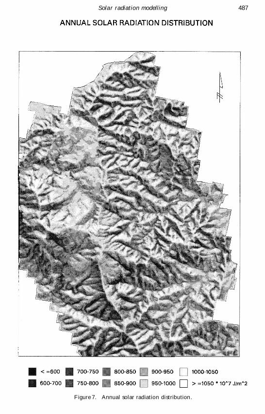
3.3. Radiation modellingSolar radiation was calculated every 30 minutes and integrated to give monthly

values. Distribution of shortwave radiation over the study site for the whole year isshown in ® gure 7 and seasonal variations are shown in ® gure 8. Figure 7 shows aconsiderable range in shortwave radiation received over the area, the range being

Figure 6. Mean deviations in insolation at each time interval from values obtained usingone minute intervals.


Figure 7. Annual solar radiation distribution.

L . Kumar et al.488

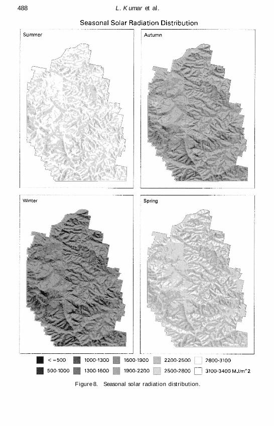
Figure 8. Seasonal solar radiation distribution.


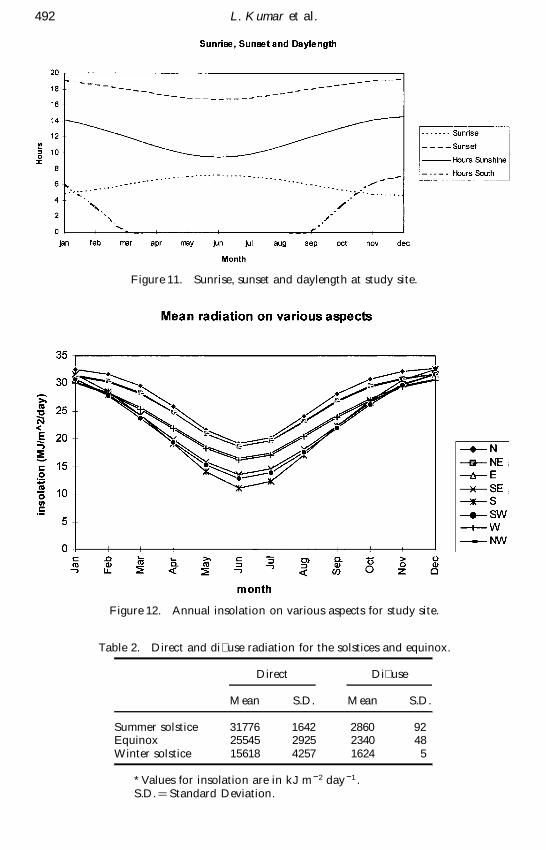
from 3647 MJ m Õ 2 to 11253 MJ m Õ 2 per year. There are also substantial areas whichreceive no direct radiation at all during the winter season, as shown in ® gure 8. Themonths of November, December and January receive the most radiation and theradiation is fairly evenly spread over all aspects, especially for ¯ atter grid cells. Thevariation in solar radiation for di� erent aspect and slope gradients are shown as® gures 9 and 10. On an annual basis, northern facing slopes generally receive farmore radiation than the south facing slopes. In many places the south facing slopesare fairly poorly irradiated, receiving only about half the shortwave radiation of thenorthern slopes. Such variations would surely have a signi® cant e� ect on the heatbudget of di� erent sites, thus in¯ uencing latent and sensible heat ¯ uxes. At slopesgreater than about 20 ß , radiation data have a higher variance with the northernslope receiving the highest radiation. It is also interesting to note that southernaspects receive a lot of radiation during the summer months. The reason for this isthat during these months the hours of sunshine are almost equal between thenorthern and southern halves of the sky. The Sun rises in the southern half, andduring the course of the day, traverses through the southern half, crossing over tothe northern side around 8 2́0 am and then back to the southern side around 3 4́0pm, before setting. In summer the Sun is also much higher in the sky, thus reducingthe shadow e� ects on southern aspects. Figure 11 shows the sunrise, sunset, daylengthand the division of hours between the northern and southern halves of the sky.

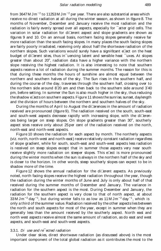
During the months of April to August the di� erences in the amount of radiationreceived are pronounced ( ® gure 9). The radiation received on the south, south-eastand south-west aspects decrease rapidly with increasing slope, with the di� eren-ces being larger on steep slopes. On slope gradients greater than 30 ß , southerlyaspect sites receive only about 25 per cent of the radiation received on the north,north-east and north-west aspects.

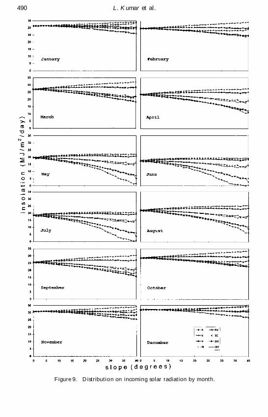
Figure 10 shows the radiation for each aspect by month. The northerly aspects(viz. north, north-west and north-east) receive relatively constant radiation regardlessof slope gradient, while for south, south-east and south-west aspects less radiationis received on steep slopes except that in summer those aspects very near southreceive slightly more radiation on steeper slopes. This e� ect is more pronouncedduring the winter months when the sun is always in the northern half of the sky andis closer to the horizon. In other words, steep southerly slopes can expect to be inshadow more of the time.

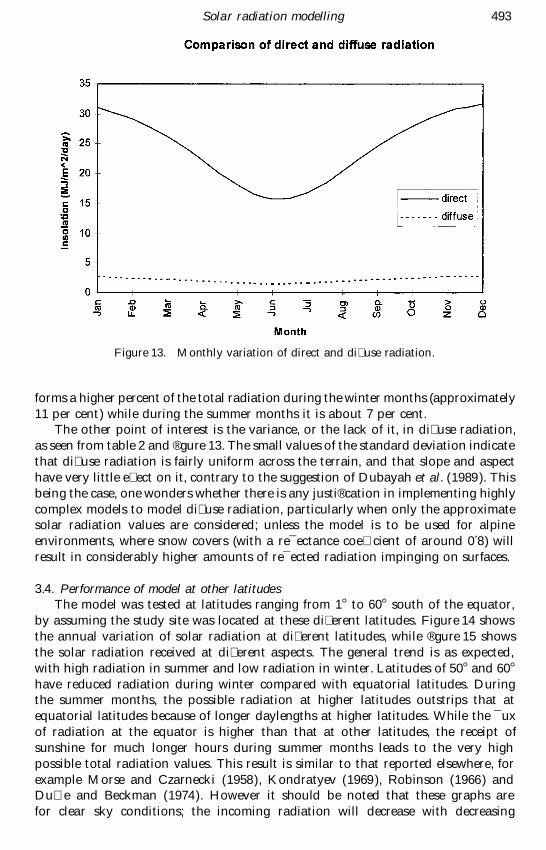
Figure 12 shows the annual radiation for the di� erent aspects. As previouslynoted, north facing slopes receive the highest radiation throughout the year, thoughthe radiation during the winter months of June and July is only about half of thatreceived during the summer months of December and January. The variance inradiation for the southern aspect is the most. During December and January, theradiation for the southern aspect is very close to that of north aspect, at about33 MJ m Õ 2 day Õ 1, but during winter falls to as low as 11 MJ m Õ 2 day Õ 1 , which isonly a third of the summer value. Radiation received by the other aspects lies betweenthe north and south aspects for most of the year, except in summer when they aregenerally less than the amount received by the southerly aspect. North east andnorth west aspects receive almost the same amount of radiation, as do east and westaspects, and south-east and south-west aspects.

3.3.1. Di� use and re¯ ected radiationUnder clear skies, direct shortwave radiation (as discussed above) is the most

important component of the total global radiation as it contributes the most to the

L . Kumar et al.490

Figure 9. Distribution on incoming solar radiation by month.


Figure 10. Variation of incident solar radiation by aspect.

energy balance. Apart from direct shortwave radiation, other components whichcontribute to the total radiation are the di� use and re¯ ected radiation.

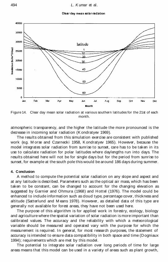
As the re¯ ected insolation was fairly small it was added to the di� use componentand henceforth the term total di� use radiation will be used to denote the sum of thetwo. Table 2 shows the magnitudes of the direct and di� use radiation for the solsticesand equinox and ® gure 13 shows the variation of both direct and di� use radiationover the year.

The total di� use radiation is between 8 and 11 per cent of the direct insolationand lies within the range given in the literature (Kondratyev 1969). Di� use radiation

L . Kumar et al.492

Figure 11. Sunrise, sunset and daylength at study site.

Figure 12. Annual insolation on various aspects for study site.

Table 2. Direct and di� use radiation for the solstices and equinox.

Direct Di� use

Mean S.D. Mean S.D.

Summer solstice 31776 1642 2860 92Equinox 25545 2925 2340 48Winter solstice 15618 4257 1624 5

*Values for insolation are in kJ m Õ 2 day Õ 1 .S.D.=Standard Deviation.


Figure 13. Monthly variation of direct and di� use radiation.

forms a higher percent of the total radiation during the winter months (approximately11 per cent) while during the summer months it is about 7 per cent.

The other point of interest is the variance, or the lack of it, in di� use radiation,as seen from table 2 and ® gure 13. The small values of the standard deviation indicatethat di� use radiation is fairly uniform across the terrain, and that slope and aspecthave very little e� ect on it, contrary to the suggestion of Dubayah et al. (1989 ). Thisbeing the case, one wonders whether there is any justi® cation in implementing highlycomplex models to model di� use radiation, particularly when only the approximatesolar radiation values are considered; unless the model is to be used for alpineenvironments, where snow covers (with a re¯ ectance coe� cient of around 0 8́) willresult in considerably higher amounts of re¯ ected radiation impinging on surfaces.

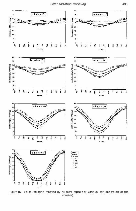
3.4. Performance of model at other latitudesThe model was tested at latitudes ranging from 1 ß to 60 ß south of the equator,

by assuming the study site was located at these di� erent latitudes. Figure 14 showsthe annual variation of solar radiation at di� erent latitudes, while ® gure 15 showsthe solar radiation received at di� erent aspects. The general trend is as expected,with high radiation in summer and low radiation in winter. Latitudes of 50 ß and 60 ßhave reduced radiation during winter compared with equatorial latitudes. Duringthe summer months, the possible radiation at higher latitudes outstrips that atequatorial latitudes because of longer daylengths at higher latitudes. While the ¯ uxof radiation at the equator is higher than that at other latitudes, the receipt ofsunshine for much longer hours during summer months leads to the very highpossible total radiation values. This result is similar to that reported elsewhere, forexample Morse and Czarnecki (1958), Kondratyev (1969 ), Robinson (1966) andDu� e and Beckman (1974). However it should be noted that these graphs arefor clear sky conditions; the incoming radiation will decrease with decreasing

L . Kumar et al.494

Figure 14. Clear day mean solar radiation at various southern latitudes for the 21st of eachmonth.

atmospheric transparency, and the higher the latitude the more pronounced is thedecrease in incoming solar radiation (Kondratyev 1969).

The results obtained from this simulation exercise are consistent with publishedwork (e.g. Morse and Czarnecki 1958, Kondratyev 1965). However, because themodel integrates solar radiation from sunrise to sunset, care has to be taken in itsuse to calculate radiation for polar latitudes where daylengths run into days. Theresults obtained here will not be for single days but for the period from sunrise tosunset, for example at the south pole this would be around 186 days during summer.

4. Conclusion

A method to compute the potential solar radiation on any slope and aspect andat any latitude is described. Parameters such as the optical air mass, which has beentaken to be constant, can be changed to account for the changing elevation assuggested by Garnier and Ohmura (1968 ) and Hottel (1976). The model could beenhanced to include information such as cloud type, percentage cover, thickness andaltitude (Satterlund and Means 1978). However, as detailed data of this type aregenerally not available for forest areas, they have not been used here.

The purpose of this algorithm is for applied work in forestry, ecology, biologyand agriculture where the spatial variation of solar radiation is more important thancalibrated values. The accuracy and the reliability with which a meteorologicalvariable should be measured and operated vary with the purpose for which themeasurement is required. In general, for most research purposes, the statement ofaccuracy is intended to ensure data compatibility in both space and time (Dogniaux1994); requirements which are met by this model.

The potential to integrate solar radiation over long periods of time for largeareas means that this model can be used in a variety of areas such as plant growth,


Figure 15. Solar radiation received by di� erent aspects at various latitudes (south of theequator).

L . Kumar et al.496

species location, water balance studies, biodiversity and identi® cation of possible¯ ora and fauna sites, although it is used here to map topographic variations in directshortwave radiation.

It must be added that, while the model successfully computes the solar radiation,the output will only be as good as the raw data supplied. In this case the model’saccuracy will greatly depend on the accuracy of the DEM used. Errors in the DEMwill lead to errors in the computed values of aspect and slope and these have adirect e� ect on the calculation of solar radiation. The other assumption of theatmosphere being uniform will have an insigni® cant e� ect on calculated radiationvalues as only clear sky radiation is being modelled.

Acknowledgement

This work was partly supported by an Australian Research Council CollaborativeGrant with Genasys II Pty Ltd and the New South Wales Land Information Centre.

References

A· ngstrom, A. K ., 1924, Solar and terrestrial radiation. Quarterly Journal of RoyalMeteorological Society, 50, 121± 125.

Barry, R. G ., 1981, Mountain Weather and Climate (New York: Methuen).Buffo, J., Fritschen, L. J., and Murphy, J. L., 1972, Direct solar radiation on various slopes

from 0 ß to 60 ß North Latitude. U.S. Forest Service Paci® c Northwest Forest RangeExperimental Station Research Paper PNW-142.

Cartwright, T. J., 1993, Modelling the World in a Spreadsheet: Environmental Simulation ona Microcomputer (Baltimore: Johns Hopkins University Press).

D ickinson, W . C., and Cheremisinoff, P. N ., 1980, Solar Energy Technology Handbook(London: Butterworths) .

Dogniaux, R., 1994, Prediction of Solar Radiation in Areas with a Speci® c Microclimate,(Dordrecht: Kluwer Academic Publishers) .

Dubayah, R., 1992, Estimating net solar radiation using Landsat Thematic Mapper anddigital elevation data. Water Resources Research, 28, 2469± 2484.

Dubayah, R., Dozier, J., and Davis, F., 1989, The distribution of clear-sky radiation overvarying terrain, in Proceedings of International Geographic and Remote SensingSymposium (Neuilly, France: European Space Agency) 2, pp. 885± 888.

Dubayah, R., and Rich, P. M ., 1995, Topographic solar radiation models for GIS. InternationalJournal of Geographical Information Systems, 9, 405± 419.

Duffie, J. A., and Beckman, W . A., 1974, Solar Energy Thermal Processes (New York: JohnWiley & Sons).

Duffie, J. A., and Beckman, W . A., 1991, Solar Engineering of Thermal Processes (New York:John Wiley & Sons).

Duguay, C. R., 1993, Radiation modelling in mountainous terrain: review and status. MountainResearch and Development, 13, 339± 357.

Duncan, C. H ., W illson, R. C., Kendall, J. M ., Harrison, R. G ., and H ickey, J. R., 1982,Latest rocket measurements of the solar constant. Solar Energy, 28, 385± 390.

Fleming, P. M ., Austin, M . P., and N icholls, A. O., 1995, Notes on a Radiation Index foruse in studies of aspect e� ects on radiation climate. CSIRO Technical Bulletin (InPress) Division of Water Resources, Canberra.

Forster, B. C., 1984, Derivation of atmospheric correction procedures for LANDSAT MSSwith particular reference to urban data. International Journal of Remote Sensing,5, 799± 817.

Frank, E. C., and Lee, R., 1966, Potential solar beam irradiation on slopes: Tables for 30 ßto 50 ß latitude. U.S. Forest Services Rocky Mountain Forest Range Experimental StationPaper R M-18 .

Frouin, R., Lingner, D . W ., Gautier, C., Baker, K . S., and Smith, R. C., 1989, A simpleanalytical formula to compute clear sky total and photosynthetically available solarirradiance at the ocean surface. Journal of Geophysical Research, 94, 9731± 9742.


Garnier, B. J., and Ohmura, A., 1968, A method of calculating the direct shortwave radiationincome of slopes. Journal of Applied Meteorology, 7, 796± 800.

Gates, D . M ., 1980, Biophysical Ecology (New York: Springer-Verlag) .Glover, J. G ., and McCulloch, J. S. G ., 1958, The empirical relation between solar radiation

and hours of bright sunshine in the high altitude tropics. Quarterly Journal of RoyalMeteorological Society, 84, 56± 60.

Hottel, H . C., 1976, A simple model for estimating the transmittance of direct solar radiationthrough clear atmospheres. Solar Energy, 18, 129± 134.

Jansen, T. J., 1985, Solar Engineering Technology (New Jersey: Prentice Hall).Kondratyev, K . Ya., 1965, Radiative Heat Exchange in the Atmosphere (New York:

Pergamon Press).Kondratyev, K . Ya., 1969, Radiation in the Atmosphere (New York: Academic Press).Kreith, F., and Kreider, J. F., 1978, Principles of Solar Engineering (New York: McGraw-

Hill ).Liu, B. Y., and Jordan, R. C., 1960, The interrelationship and characteristic distribution of

direct, di� use and total solar radiation. Solar Energy, 4, 1 ± 19.Monteith, J. L., and Unsworth, M . H ., 1990, Principles of Environmental Physics (London:

Edward Arnold ).Morse, R. N ., and Czarnecki, J. T., 1958, Flat plate solar absorbers: The e� ect on incident

radiation of inclination and orientation. CSIRO Report E.D. 6, Melbourne, Australia.Nunez, M ., 1980, The calculation of solar and net radiation in mountainous terrain. Journal

of Biogeography, 7, 173± 186.Richards, J. A., 1993, Remote Sensing Digital Image Analysis: An Introduction (Berlin:

Springer Verlag).Robinson, N ., 1966, Solar Radiation (Amsterdam: Elsevier Publishing Company).Satterlund, D . R., and Means, J. E., 1978, Estimating solar radiation under variable cloud

conditions. Forest Science, 24, 363± 373.Sayigh, A. A. M ., 1977, Solar Energy Engineering (New York: Academic Press).Skidmore, A. K ., 1990, Terrain position as mapped from a gridded digital elevation model.

International Journal of Geographical Information Systems, 4, 33± 49.Swift, L. W ., 1976, Algorithm for solar radiation on mountain slopes. Water Resources

Research, 12, 108± 112.Turner, R. E., and Spencer, M . M ., 1972, Atmospheric model for correction of spacecraft

data. In Proceedings of 8th International Symposium on Remote Sensing of theEnvironment, (Ann Arbor: E.R.I.M.), pp. 895± 934.

Wehrli, C., 1985, Extra-terrestrial Solar Spectrum. Publication No. 615 (Davos Dorf: WorldRadiation Centre).

W illiams, L. D ., Barry, R. G ., and Andrews, J. T., 1972, Application of computed globalradiation for areas of high relief. Journal of Applied Meteorology, 11, 526± 533.

radiatia solara incidenta

Documents