ASD TECtHNICAI. REPORT 61-1.19 (Q •PART I ... "

RADIATION HEAT TRANSFER ANALYSIS FORSPACE VEHICLES

J. A. STEVENSON1. C. GRAFTON

SPACE AND INFORMATION SYSTEMS DIVISIONNORTH AMERICAN AVIATION, INC.

SID 61-91

DECEMBER 1961

FLIGHT ACCESSORIES LABORATORYCONTRACT AF 33(616)-7635

PROJECT No. 6146TASK No. 61118

AERONAUTICAL SYSTEMS DIVISIONAIR FORCE SYSTEMS COMMAND

UNITED STATES AIR FORCEWRIGHT-PATTERSON AIR FORCE BASE, OHIO

5 '

NOTICES

When Government drawings, specifications, or other data are used for any purposeother than in connection with a definitely related Government procurement operation, theUnited States Government thereby incurs no responsibility nor any obligation whatsoever;and the fact that the Government may have formulated, furnished, or In any way suppliedthe said drawings, specifications, or other data, is not to be regarded by implication orotherwise as in any manner licensing the holder or any other person or corporation, orconveying any rights or permission to manufacture, use, or sell any patented inventionthat may in any way be related thereto.

Qualified requesters may obtain copies of this report from the Armed Services Tech-nical Information Agency, (ASTIA), Arlington Hall Station, Arlington 12, Virginia.

This report has been released to the Office of Technical Services, U. S. Departmentof Commerce, Washington 25, D. C., for sale to the general public.

Copies of ASD Technical Reports and Technical Notes should not be returned to theAeronautical Systems Division unless return is required by security considerations, con-tractual obligations, or notice on a specific document.

FOREWORD

This is one of a series of reports which summarizes the first 6-munthphase of a planned 3-year study of thermal and atmospheric control systemnsof manned and unmanned space vehicles. The study was conducted by theSpace and Information Systems Division of North American Aviation, Inc.under contract AF 33(616)-7635, and was sponsored by the Flight AccessoriesLaboratory of Aeronautical Systemns Division (formerly Wright AirDevelopment Division). The Los Angeles Division of North AmericanAviation, Inc., and AiResearch Manufacturing Company were subcontractorsin the study effort.

The reports covering the results of the first 6-month period of thisF study are listed below. Because of the intention to revise, amplify, and

extend the material presen~ted, each report has been designated as Part 1.

In addition to publishing these subsequent parts, new phases of the study will

result in additional reports.

ASD TR 61- 164 Environmental Control Systems Selecticon for(Part I) Unmanned Space Vehicles (secret)F ASD TR 6 1-240 Environmental Control Systems Selection for(Part I) Manned Space Vehicles, Volume I

(unclassified) and Volume II (secret)

ASD TR 61-161 Space Vehicle Environmental Control(Part I) Requirements Based on Equipment and

Physiological Criteria

ASD TR 61-119 Radiation Heat Transfer Analysis for(Part I) Space Vehicles

ASD TR 61-30 Space Radiator Analysis and Design(Part I)

ASD TR 61-176 Integration and Optimization of'(Part I) Space Vehicle Environmental Control Systems

ASD TR 61-162 Analytical Methods for Space Vehicle(Part I) Atmospheric Control Processes

ASD TR 61-119 Pt I iii

The thermal and atmospheric control program was under the directionof A. L. Ingelfinger and Lieutenant N. P. Jeffries of the Environmental Control

Section, Flight Accessories Laboratory. E. A. Zara of the Environmental

Control Section acted as monitor of this report. A. C. Martin served asproject engineer at S&ID. The radiation heat transfer studies were conducted

by J. A. Stevenson and J. C. Grafton.

Appreciation is expressed to the Astronautics and Fort Worth Divisions

of Convair (General Dynamics Corporation) and, in particular, John C,Ballinger of the Astronautics Division. Much of the data included in this

report was obtained from Convair.

The authors also wish to express their appreciation to G.A. McCue of

the Aero-Space Laboratories of S&ID who contributed a major part to theorbiting space vehicle studies at S&ID.

ASD TR 61-119 Pt I -iv-

ABSTRACT

ThisLdocument covers problems associated with one part of tih thermaland atmospheric control study-toj analysis of radiation heat transfer inspace. The basic theory of radiation heat transfer and tide thermal radiationenvironment in space a'e described. Analysis techniques aVe included forcalculating space vehicle surface temperatures and for solving radiation heattransfer problems in generaj. Tabulated configuration factor data andemittance data ate presenteA

(,pp)( fig.) M;lbS..) ( ref.)

PUB LICATION REVIEW

This report has been reviewed and is approved.

FOR THE COMMANDER:

WILLIAM C. SAVAGEChief, Environmental BranchFlight Accessories Laboratory

ASD TR 61-119 Pt I

~----V-~

CONTENTS

Section Page

INTRODUCTION ... 1

Study Program . 1Role of Radiant Heat Transfer Analysis 1

II GLOSSARY OF RADIATION TERMS .. 3

III THEORY OF RADIATION HEAT TRANSFER 7Basic Concepts of Thermal Radiation . . 7Radiation Laws .. a 7Radiant Heat Exchange Between Surfaces 19

IV THERMAL RADIATION ENVIRONMENT IN SPACE . 25Direct Solar Radiation 25Reflected Solar Radiation 29Planetary Emitted Radiation 31

V SPACE VEHICLE "JURFACE TEMPERATURE ANALYSIS 33Introduction 33Simplified Space Radiation Analysis . 35

Nomenclature 35Heat Balance 36Analysis Description . 37

IBM 7090 Program for Transient Heat TransferAnalysis of Orbiting Space Vehicles 41

Nomenclature 41Orbital Mechanics 44Solution for Shadow Intersection Points . 46Vehicle Configuration 57Geometric Configuration Factors 58Temperature Determination , 69Program Listing and Deck Setup 72

Space Thermal Environment Study 77

Nomenclature 77Planetary Thermal Emission 79Planetary Reflected Solar Radiation 92

Discussion of Assumptions 115Simplified Space Radiation Analysis 115IBM 7090 Program for Transient Heat Transfer

Analysis of Orbiting Space Vehicles 116Space Thermal Environment Study 118

ASD TR 61-119 Pt I -vii-PREVIOUS PAGE

ISBLANKW

Section Page

VI TECHNIQUES FOR RADIATION HIAT TRANSFER PROBLEMSOLUTION 1. .I21

General Analog Heat Transfer I nalysis Methods 121Nomenclature 121Electric Circuit Analogy 122Steady-State and Transient Pioblem Solution 1Z2

Radiation Heat Transfer Analysis M0ethods 127Nomenclature 127Radiosity Analog Method 127Commonly Used Methods 131Comparison of Analytical Methods 132

Ray Tracing Analysis Method 141Nomenclature 141Radiant Interchange Analysis 141Digital Computation 146

Discussion of Assumptions 151

VII CONFIGURATION FACTOR STUDIES AND DATA 153Configuration Factor Evaluation 153Tabulated Data 163

Data of Report NACA TN 2836 .. 163Data of Convair (Fort Worth) Study 164Data of ASME Paper 56-A-144 187Discussion 209

Configuration Factor Development 217IBM 7090 Program (Geometric Configuration

Factors) .. 17Unit Sphere Method. (Differential-Finite

Configuration Factor) 218Discussion of Assumptions 221

VIII EVALUATION STUDIES 223Nomenclature 223Variables Selected 223Rotating Sphere Evaluation 224Comparison of Rotating Sphere and Flat Plate 240"Cyclic Temperature Variation of Eight-Sided Prism 244Discussion of Assumptions 248

IX CONCLUSIONS . .251Analysis Techniques 251Problem Areas Z51

SASD TR 61-119 Pt -viii-

Section Page

X ANNOTATED BIBLIOGRAPHY 2. 55Periodicals 2. 55Reports and Papers . 261Books *. 268

XI REFERENCES . .. 273

APPENDIXES

PageAppendix

A Tables of Emissivity and Absorptivity 277B Planetary Thermal Emission and Planetary Reflected

Solar Radiation Incident to Space Vehicles 297

ASD TR 61-119 Pt I -ix-

ILLUSTRATIONS

Figure Page

1 Electromagnetic Spectrum . . . 8

2 Energy Distribution of Black Body IF. 93 Representation of Lambert's Cosine Law . . 114 Theoretical and Experimental Values for Ratio of

Hemispherical to Normal Ernissivity I .IF 145 Absorption by Optical Interference I. 156 Cavity Absorption . . .. 167 Effect of Sandblasting on Total Emissivity 178 Reflective Surfaces IF. . . I 18

9 Fresnel Reflection IF. I I 19

10 Heat Exchange Between Two Surfaces . 2011 Solar Radiation at Various Distances From Sun IF 2612 Spectral Energy Curve of Sun ... . 2713 Space Vehicle Orientation . . . . 3614 Elements of Elliptic Orbits . . . . .. 45i5 Shadow Geometry (Projection Upon Orbital Plane) 4716 Eclipse Time as Function of Date (Zero Eccentricity,

0-Degree Inclination) . . I 4917 Eclipse Time as Function of Date (Zero Eccentricity,

33-Degree Inclination) F . 5018 Eclipse Time as Function of Date (Zero Eccentricity,

48-Degree Inclination) . . 51

19 Eclipse Time as Function of Date (Zero Eccentricity,65-Degree Inclination) 52

20 Eclipse Time as Function of Date (Zero Eccentricity,80-Degree Inclination) 53

21 Effect of Variation in Eccentricity on Eclipse Time asFunction of Date . . I I 54

22 Effect of Variation in Launch Time on Eclipse Time asFunction of Date . . . 55

23 Seasonal Boundaries of Shadow Intersection Characteristics . 5624 Satellite Configurations Used in Transient Temperature

Analysis .. . . 5925 Planetary Emission Form Factor (Rotating Sphere) . . 60

26 Form Factor Determination (Case I) . . . 6327 Form Factor Determination (Case II) . . . 6528 Form Factor Determination (Case I1) I IF 6729 Space Vehicle Heat Balance I 70

ASD TR61-119 Pt Ixi

PR VO US PAGEI LANK'M

Figure Page

30 Satellite Temperature Determination 7331 Deck Setup .. . 74

32 Main Program Flow Diagram .. . .. 7533 Geometry of Planetary Thermal Emission to Sphere . 8134 Geometric Factor for Earth Thermal Emission Incident

to Sphere Versus Altitude . . . ... 82

35 Geometry of Planetary Thermal Emission to Cylinder . 83

36 Geometric Factor for Earth Thermal Emission Incident toCylinder Versus Altitude as Function of Attitude Angle. . 85

37 Geometry of Planetary Thermal Emission to Hemisphere . 8638 Geometric Factor for Earth Thermal Emission Incident to

Hemisphere Versus Altitude as Function of Attitude Angle . 8839 Geometry of Planetary Thermal Emission to Flat Plate . 9040 Geometric Factor for Earth Thermal Emission Incident to

Flat Plate Versus Altitude as Function of Attitude Angle . 9341 Geometry of Planetary Reflected Solar Radiation to Sphere 9442 Cases for Limits of Integration in Reflected Solar Radiation

to Sphere . . . .... 9643 Geometric Factor for Earth Reflected Solar Radiation Incident

to Sphere Versus Altitude as Function of Sun Angle 9844 Geometry of Planetary Reflected Solar Radiation to Cylinder . 9945 Geometry of Planetary Reflected Solar Radiation to

Hemisphere . . . . . .10246 Geometry of Planetary Reflected Solar Radiation to Flat Plate. 10547 Thermal Network for Insulated Wire . . . . 12348 Simplified Thermal Network for Insulated Wire . . , 12349 Thermal Network for Single Node, Slngle Resistor Transient

Problem . . . . . . .. 12450 Thermal Network for Temperature Distribution Versus Time

in Slab . . . . . . .. 12551 Radiosity Analog Network for Four-Sided Enclosure 130

52 Conventional Analog Network for Four-Sided Enclosure 13053 Parallel Disks .. . . 13254 Radiosity Network for Problem 1 134

55 Radiosity Network for Determining Equivalent Conductance 13556 Radiosity Network for Problem 2 . . . 139

57 Geometry for Calculation of Configuration Factor for TwoMutually Perpendicular Surfaces . . . . 154

58 Diagram of Infinite Enclosure . ,,.156

59 Diagram of Differential Area and Infinitely Long Surface . . 157

60 Differential Area Shape Factor for Two-Dimnensional Case 15961 Shape Modulus From Differential Area to Lune 16162 Nodes on Parallel Planes 165

"63 Nodes on Skewed Planes 166

ASD TR 61-119 Pt I -xii-

Figure Page

64 Nodes on Plane and Parallel Cylinder 169

65 Nodes on Concentric Cylinders . 172

66 Nodes on Parallel Cylinders . 174

67 Nodes on Cylinder and Skewed Plane . 176

68 Nodes on Cylinder (Internal) . 179

69 Nodes on Plane and Sphere . .18170 Sphere-Cone-Cylinder Configuration 18Z71 Rectangular Box Configuration . 186

72 Form Factor From Outer Cylinder to Inner Cylinder 19773 Form Factor From Outer Cylinder to Itself 19774 Geometry for Yamauti's Modified Reciprocity Relationship 21075 Diagram of Infinitely Long Enclosure . ..211

76 Diagrams of Configuration Factor Algebra .2 . 1377 Diagram of Unit Sphere Method for Determining Configuration

Factor . .2. . 19

78 Variation of Orbital Height for Rotating Sphere 225

79 Variation of Orbital Inclination for Rotating Sphere . . 22780 Variation of Emissivity for Rotating Sphere

(Absorptivity 0. 10) ... . .229

81 Variation of Emissivity for Rotating Sphere(Absorptivity 0. 50) . . 230

82 Variation of Emissivity for Rotating Sphere(Absorptivity 1. 0) . . 231

83 Variation of Mass for Rotating Sphere 233

84 Variation of Internal Heat Load for Rotating Sphere 23685 Variation of Absorptivity-to-Emissivity Ratio for Rotating

Sphere (Earth Albedo 0. 2) . . . . 237

86 Variation of Absorptivity-to-Emissivity Ratio for RotatingSphere (Earth Albedo 0. 5) . . 238

87 Variation of Absorptivity-to-Emissivity Ratio for RotatingSphere (Earth Albedo 0. 8) 2. . 39

88 Variation of Absorptivity-to-Emi3sivity Ratio for RotatingSphere [Solar Constant 433 Btu/(Hour) (Square Foot)] • 241

89 Variation of Absorptivity-to-En-issivity Ratio for RotatingSphere [Solar Constant 453 Btu/(Hour) (Square Foot)] . 242

90 Comparison of Rotating Sphere and Flat Plate 2. . 4391 Diagram of Earth-Oriented Eight-Sided Prism 24592 Cyclic Temperature Variation of Earth-Oriented Eight-Sided

Prism . . .. . Z46

ASD TR 61-119 PtI -xiii-

TABLES

Table Page

I Solar Radiation Temperatures . . . . . .. . 282 Energy Distribution of Solar Electromagnetic Radiation . . 283 Luminous Reflectance of Various Earth Objects . . . . 304 Planetary Albedos . . . . . . . . . . 31

5 Planetary Temperatures . . . . . . . ..*32

6 Study Variables for Rotating Sphere . . . . . 2247 Variation of Orbital Height for Rotating Sphere . . . . 2268 Variation of Surface Finish for Rotating Sphere . . . . 2289 Variation of Mass for Rotating Sphere .. . 232

10 Variation of Earth Albedo for Rotating Sphere . . . 23511 Variation of Solar Constant for Rotating Sphere . . . . 23512 Maximum and Minimum Temperatures for Eight-Sided Prism . 244

ASD TR 61-119Pt I Xiv-

Section I

INTRODUCTION

STUDY PROGRAM

The Thermal and Atmospheric Control Study conducted for AeronauticalSystems Division (formerly Wright Air Development Division) is an analyticaland experimiental program concerned with the problems of environmentalcontrol of future space vehicles. Three broadly defined tasks were designatedfor this study. They are:

1. Improved analysis methods for predicting the requirements forand the performance of space environmental control systems

2. Improved methods, techniques, systems, and equipment requiredfor environniental control

3. Development of criteria and techniques for the optimization ofenvironmental control systems and the integration of these systemswith other vehicle systems

To accomplish these tasks, industrial organizations and militaryestablishments were surveyed to obtain data concerned with current andfuture thermal and atmospheric control technology. Other endeavors includeevaluating existing and newly created methods of analysis, selection,integration, and optimization of control systems and components. Therefurbishment and development of existing and new analog or digital computerprograms, applicable to this study, are included. In addition, laboratoryverification of analyses and new design concepts form a part of the effortassociated with these tasks.

To guide all of the endeavors along lines which will find immediateand practical application, components and systems associated with specificvehicles were studied. The vehicles selected were representative of anumber of earth-orbital and cislunar missions. These hypothetical vehicleswere carried through preliminary design and used as thermal andatmospheric control models.

ROLE OF RADIANT HEAT TRANSFER ANALYSIS

Although transfer of heat within a space vehicle or satellite can occurby radiation, conduction, or convection, the only means by which the vehicle

Manuscript released by the authrors M'a4y 1961 for publication as anASD Technical Report.

ASD TR 61-119 Pt I - I -

can exchange heat with its environment is by radiation. Temperature controlsystems, either active or passive, must eliminate heat by radiation to space.An accurate method of radiation heat transfer analysis is therefore of primeimportance for the prediction of vehicle and component termperatures andthe performance of temperature control systems.

This report documents a study of available methods of radiation heattransfer analysis and reviews the basic principles of thermal radiation.Included in the appendix sections are tables of emissivity and reflectivity forcertain surface coatings which can be applied to space vehicles. This areais also of prime importance because even the most refined analysis tech-niques are only as accurate as the values of emittance and reflectance whichare used.

-2.

Section II

GLOSSARY OF RADIATION TRANSFER TERMS

The following terms conform in terminology and symbolicrepresentation to those most widely used in radiation heat transferliterature.

Absorptance or Ratio of absorbed radiant energy to incidentabsorptivity a radiation. Related to reflectance and

transmittance by

lea +p + rat

,Albedo, a Ratio of radiant energy reflected by planet orsatellite to that received by it. A dimensionlessdecimal equal to or less than 1. Care must betaken to avoid confusion between the albedos oftotal and visible radiant energy.

Angstrom, A Unit of measurement of wavelength of electro-magnetic waves.

1 crn= 108 10 P

Black body Hypothetical body having the characteristic ofabsorbing all radiant energy striking it andreflecting and/or transmitting none.

a = 1.0, p = r = 0

Diffuse reflection Reflection that follows Lambert's cosine law(i.e., intensity I is constant regardless ofangle). Nonmetallic surfaces are often nearlyperfect diffusive reflectors.

Emittance, c Ratio of emissive power E of a body to emissivepower Eb of a black body at the same temperature.A dimensionless decimal equal to or less than 1.Distinctions are made between difference typesof emittance.

Total emittance Emittance of the whole range of wavelengths.

-3-

gum

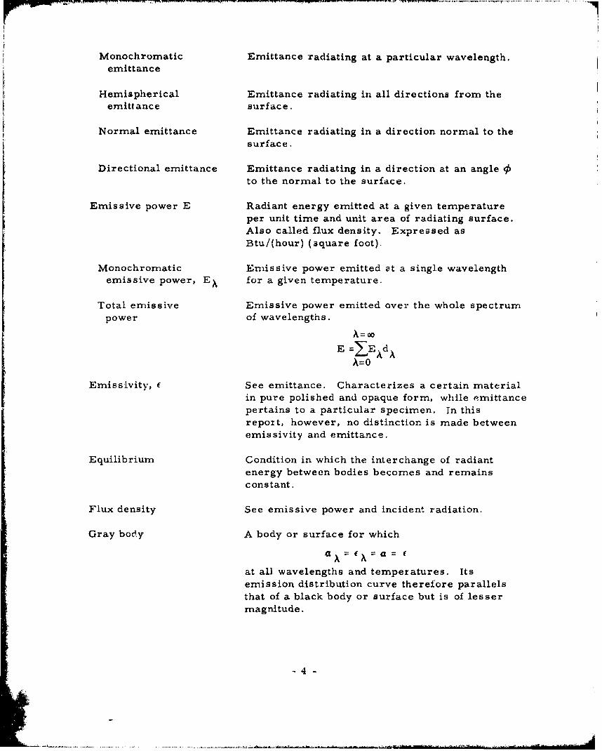
Monochromatic Emittance radiating at a particular wavelength.emittance

Hemispherical Emittance radiating in all directions from theemnittance surface.

Normal emittance Emittance radiating in a direction normal to thesurface.

Directional emittance Emittance radiating in a direction at an angle 5to the normal to the surface.

Emissive power E Radiant energy emitted at a given temperatureper unit time and unit area of radiating surface.Also called flux density. Expressed asBtu/(hour) (square foot).

Monochromatic Emissive power emitted at a single wavelengthemissive power, EX for a given temperature.

Total emissive Emissive power emitted over the whole spectrumpower of wavelengths.

A=0oE =-E A d A

A=0

Emissivity, C See emittance. Characterizes a certain materialin pure polished and opaque form, while emnittancepertains to a particular specimen. In thisreport, however, no distinction is made betweenemissivity and emittance.

Equilibrium Condition in which the interchange of radiantenergy between bodies becomes and remainsconstant.

Flux density See emissive power and incident radiation.

Gray body A body or surface for which

a - a

at all wavelengths and temperatures. Itsemission distribution curve therefore parallelsthat of a black body or surface but is of lessermagnitude.

4-

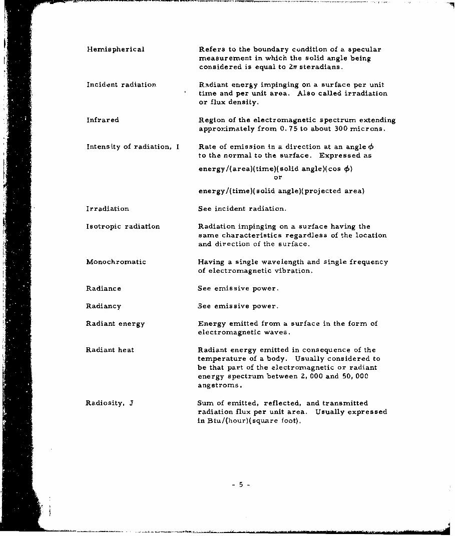
Hemispherical Refers to the boundary condition of a specularmeasurement in which the solid angle beingconsidered is equal to Za steradians.

Incident radiation Radiant energy impinging on a surface per unittime and per unit area. Also called irradiationor flux density.

"Infrared Region of the electromagnetic spectrum extendingapproximately from 0. 75 to about 300 microns.

Intensity of radiation, I Rate of emission in a direction at an angle 4,to the normal to the surface. Expressed as

energy/(area)(time)( solid angle)( cos q5)or

energy/(time)(solid angle)(projected area)

Irradiation See incident radiation.

Isotropic radiation Radiation impinging on a surface having thesame characteristics regardless of the locationand direction of the surface.

Monochromatic Having a single wavelength and single frequencyof elect rornagnetic vibration.

Radiance See emissive power.

Radiancy See emissive power.

Radiant energy Energy emitted from a surface in the form ofelectromagnetic waves.

Radiant heat Radiant energy emitted in consequence of thetemperature of a body. Usually considered tobe that part of the electromagnetic or radiantenergy spectrum between Z, 000 and 50, 000angstroms.

Radiosity, J Sum of emitted, reflected, and transmittedradiation flux per unit area. Usually expressedin Btu/(hour)(square foot).

-5

Reflectance, p Ratio of reflected to incident radiant energy.Related to absorptance and transmittance by

p +a+ r=

Spectral energy Monochromatic emissive power over the rangedistribution of the spectrum of an emitting surface.

Specular reflection Refers to reflection which occurs in such a waythat the angle between the reflected beam ofradiation and the normal to the surface equalsthe angle made by the impinging beam with thesame normal.

Stefan-Boltzmann Constant which is independent of surface andconstant, a temperature and relates heat radiated qr to

absolute temperature, area, and emissivity.The relationship is

q= aAT

Thermal radiation See radiant heat.

Transmittance, r Ratio of radiant energy transmitted through thebody to the incident radiation. Related toabsorptance, and reflectance by

r+a +p = 1

Total radiation Sum of all radiation over the entire spectrum ofemitted wavelengths.

Ultraviolet Region of the electromagnetic spectrum extendingapproximately from 0. 01 to 0. 4 micron.

Visible Region of the electromagnetic spectrum extendingapproximately from 0. 4 to 0. 75 micron.

Wavelength, A Distance measured along line of propagationbetween two points which are in phase onadjacent waves.

-6-

Section III

THEORY OF RADIATION HEAT TRANSFER*

BASIC CONCEPTS OF THERMAL RADIATION

The process of emission of radiant energy by a body, which dependson its temperature, is called thermal radiation. Each body, by virtue ofits temperature, is constantly emitting electromagnetic radiation from itssurface into the surrounding space and is absorbing radiant energyoriginating elsewhere and incident upon it. Electromagnetic radiation iscomposed of all wavelengths, including extremely short-wave secondarygamma rays and the longest radio waves. Theoretically, all bodies emitradiation over the entire electromagnetic spectrum (Figure 1).

The amount of energy emitted generally varies with wavelength in amanner similar to that shown in Figure Z. The curves give the spectraldistribution of radiation from a black body at temperatures of 2700, 1980,and 1260 R. The maximum energy emitted by a body increases as thetemperature increases, and the wavelength at which the maximum energy isradiated becomes shorter as the temperature increases.

The rate of radiation from a black, or ideal, body is proportional tothe fourth power of its absolute temperature. For other bodies, the rate ofradiation is also proportional to the fourth power of their absolute temperature,but the magnitude varies depending on material, surface condition, andtemperature. The rate of emission of energy per unit area for non-black-body materials is never greater than the rate of energy emission per unit areafrom a black body. For this reason, the black body is used as a standardor reference, and emission from other bodies is compared with it.

RADIATION LAWS

Kirchhoff's Law

Kirchhoff, in 1860, proposed a system consisting of a completelyenclosed hollow space into which a thin plate is placed, the enclosure andplate being at the same temperature.

*The material in this section of the report was gathered from ReferencesI through 5.

-7-

Uo> o

0.

-4

-44

4-

"j 0

- bII4

0

- ____________ Z "-"< :> 0

o C

=•-8--

32 -

28

- 24

~20I14• 2700 R

S0

U

4 12

0

0 2 4 6 8 10 12

WAIVELENGTH, A (MICRONS)

Figure 2. Energy Distribution of Black Body

"-9-

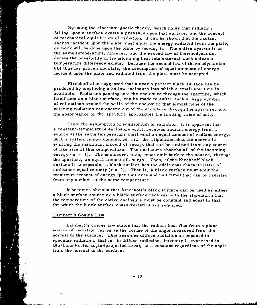
By using the electromagnetic theory, which holds that radiationfalling upon a surface exerts a pressure upon that surface, and the conceptof mechanical equilibrium of radiation, it can be shown that the radiantenergy incident upon the plate must equal the energy radiated from the plate,or work will be done upon the plate by moving it. The entire system is atthe same temperature, however, and the second law of thermodynamicsdenies the possibility of transforming heat into external work unless atemperature difference exists. Because the second law of thermodynamicshas thus far proven inviolate, the assumption of equal amounts of energyincident upon the plate and radiated from the plate must be accepted.

Kirchhoff also suggested that a nearly periect black surface can beproduced by employing a hollow enclosure into which a small aperture isavailable. Radiation passing into the enclosure through the aperture, whichitself acts as a black surface, can be made to suffer such a large numberof reflections around the walls of the enclosure that almost none of theentering radiation can escape out of the enclosure through the aperture, andthe absorptance of the aperture approaches the limiting value of unity.

From the assumption of equilibrium of radiation, it is apparent thata constant-temperature enclosure which receives radiant energy from asource at the same temperature must emit an equal amount of radiant energy.Such a system is now considered with the stipulation that the source isemitting the maximum amount of energy that can be emitted from any sourceof like size at this temperature. The enclosure absorbs all of the incomingenergy (a = 1). The enclosure, also, must emit back to the source, throughthe aperture, an equal amount of energy. Then, if the Kirchhoff blacksurface is acceptable, a black surface has the additional characteristic ofemittance equal to unity (e = 1). That is, a black surface must emit themaximum amount of energy (per unit area and unit time) that can be radiatedfrom any surface at the same temperature.

It becomes obvious that Kirchhoff's black surface can be used as eithera black surface source or a black surface receiver with the stipulation thatthe temperature of the entire enclosure must be constant and equal to thatfor which the black surface characteristics are required.

Lambert's Cosine Law

Lambert's cosine law states that the radiant heat flux from a planesource of radiation varies as the cosine of the angle measured from thenormal to the surface. This assumes diffuse radiation as opposed tospecular radiation, that is, in diffuse radiation, intensity I, expressed inBtu/(hour)(s:lid angle)(projected area), is a constant regardless of the anglefrom the normal to the surface.

10

Consider Figure 3, letting the elemental area dA 1 represent Lambert'sdiffusely reflecting surface. When a constant density of radiation in spaceis assumed and only radiation in the visible range is considered, the areadA 1 cosS viewed from M appears equally as bright as the area dA 1 viewedfrom N, and the quantity of light falling upon any area dA 2 is directlyproportional to the area dAl cos $. These same concepts apply equally aswell to radiation of longer wavelength as they do to radiation of the visiblerange. The amount of radiant energy reaching a surface dA 2 from a blacksurface dA 1 is directly proportional to the area dA 1 cos 9.

S~N

( W.SOLID ANGLE)

0 dAl

Figure 3. Representation of Lambert's Cosine Law

True surfaces vary from this law depending upon the material. Whenthe radiation intensity of a surface follows the cosine law, the directionalemittance is independent of the angle of emission and is identical with thehemispherical emittance. Actually, the emittance of all true surfaces isdependent to a certain degree on the angle of emission.

•- 11 -

illIPOR 5IMiIU IIP.I

Stefan -Boltzmnann's Law

Stefan empirically found the relationship between the Intensity ofradiation from a black surface source and the absolute temperature of thesurface. Later, Boltzmann theoretically reduced this same relationship,stating that the heat radiated by a black body is proportional to the fourthpower of its absolute temperature, or

q = aAT 4 (1)

where

q = Total heat emitted, Btu/hr

a = Stefan-Boltzmann constant = 0. 1713 x 10-8 Btu/(hr)(sq ft)(°R4

A = Emissive area, sq ft

T = Absolute temperature, OR

For non-black bodies, the heat emitted equals the black body heatemitted multiplied by the emittance, or

q = f(aAT 4 ) (Z)where

c Emittance of non-black body

Wien's Displacement Law

For black body radiation, if the wave oi length A? at TZ is displacedfrom that of length X1 at T1, such that X2T 2 = Al T 1 , the monochromaticemissive powers at these two wavelengths are directly proportional to thefifth powers of the absolute temperatures, or

SEX T 13)

5i iNEAz T5

Wien also determined that when the temperature of a radiating blackbody increases, the wavelength corresponding to the maximum energy de-creases in such a way that the product of the absolute temperature andwavelength is a constant. (See Figure 2..) This is expressed as

XmaxT= 5216. 2 A(°R) (4)

-!12!-

Planck's Distribution Law

The present understanding of radiation and the spectrum began todevelop in 1900 when Max Planck formulated his theory of the "granular"nature of energy and developed a new kind of statistics, the quantum theory,to handle his concept mathematically. Radiant energy leaving a surface isdistributed over the entire wavelength range, and the distribution of theenergy with wavelength is a function of the temperature and nature of thesurface. The emissive power distribution at a given temperature for a black

body is given as

- 5C A

E1 (5)A eC/AT_1e 2 -

where

8 4C1 = 1. 1870 x 10 Btu p /(hr)(sq ft)

c2 = 25, 896 gUR)

e = Base of natural logarithm

Absorption and Emission of Radiant Energy

The efficacy of the surface to emit or absorb radiation is presentedin terms of emissivity and absorptivity factors. These factors are definedas the ratio of energy emitted or absorbed at each wavelength to the energyemitted or absorbed by a black body at the same temperature. These factors

are usually presented as the total or average values over all wavelengths fora particular surface.

In addition to being functions of wavelength, emissivity andabsorptivity are functions of the angle the light ray makes with the surface.

Values are reported usually in terms of the normal (perpendicular to thesurface) or hemispherical (average overall angles). The variation betweennormal and hemispherical emissivity is shown in Figure 4, as taken fromReference 3. Emissivities or absorptivities are often presented as totalhemispherical or total normal, or they are given as a function of wavelength for

normal or hemispherical radiation. Reflectance, or transmittance fortransparent materials, is sometimes given rather than absorptivity. This,of course, is simply I - a.

Absorption or emission of energy up to about 2- microns wavelengthis due primarily to raising the energy levels of the orbital electrons. Theseexcited electrons then give up their energy usually in the form of molecularvibrational energy or fluorescence. Most electronic transitions involve

- 13 -

1.4-

>'1. 3ALUMINUM

-CHROMIUM

NICKEL (POLISHED)1.2 NICKEL (DULL)

0z/ALUMINUM

)PAINT

1BISMUTH

Wz 1.00

H COPPER (OXIDIZED)@10

GLASS@

0. 90 0.2 0.4 o. 6 0.8 1.0

NORMAL EMISSIVITY, E N

Figure 4. Theoretical and Experimental Values for

Ratio of Hemispherical to Normal Ernissivity

-14-

relatively large energy steps, and the temperature of the surface thereforehas little effect on absorption in this range. Because almost all the solarenergy lies in the wavelength below 2 microns, solar absorptivity asshould be nearly constant with surface temperature. Some minor effectsare noted with temperature, caused by such factors as crystal structurechanges.

Absorption or emission beyond 2 microns is due to raising thevibrational and kinetic energy levels of the molecules themselves. Organicmaterials are more sensitive to vibrational absorption than electricallyconductive materials. Semiconductor materials are generally transparentto a large portion of the infrared region. The absorptivity or emissivity ofany material varies with wavelength, and this variation is not the same fordifferent mate rials.

Absorption can also occur by optical interference, where light isreflected 90 degrees out of phase from successive layers of a multilayer ,coating. This interference results in absorption of the energy ratherthan reflection. The coatings are usually alternate thin layers of metaland a dielectric, as shown schematically in Figure 5. For maximumabsorption, the coating should be applied in thicknesses of one-quarterwavelength. If the thickness is one-half wavelength, the rays reinforcerather than cancel each other. By proper choice of materials andthicknesses, narrow or broad bands of light can be absorbed.

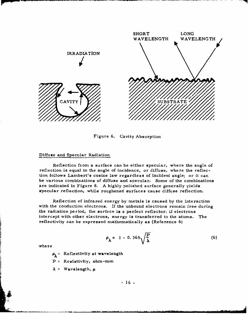
Another technique for achieving high absorption is to allow multiplereflections to take place before the radiant energy leaves the surface.This can be accomplished by placing cavities on the surfaces, either bysandblasting or by using wire mesh, honeycomb, or similar techniques.This effect is shown schematically in Figure 6. If the holes are small,only short wavelength radiation is absorbed and the surface appears flat tolong wavelength radiation. The effect of sandblasting is to increaseemissivity by about 10 percent, as shown in Figure 7 for oxidized 310stainless steel.

DIELECTRIC

METAL COATING

DIE L.C TRiV

SUBSTRATE

Figure 5. Absorption by Optical Interference

-15-

SHORT LONGWAVELENGTH WAVELENGTH/

IRRADIATION

/ 1 /

CAVITY SUBST ATE

Figure 6. Cavity Absorption

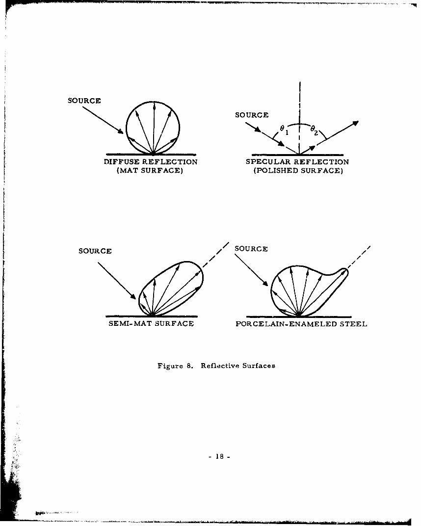
Diffuse and Specular Radiation

Reflection from a surface can be either specular, where the angle ofreflection is equal to the angle of incidence, or diffuse, where the reflec-tion follows Lambert's cosine law regardless of incident angle; or it canbe various combinations of diffuse and specular. Some of the combinationsare indicated in Figure 8. A highly polished surface generally yieldsspecular reflection, while roughened surfaces cause diffuse reflection.

Reflection of infrared energy by metals is caused by the interactionwith the conduction electrons. If the unbound electrons remain free duringthe radiation period, the surface is a perfect reflector; if electronsintercept with other electrons, energy is transferred to the atoms. Thereflectivity can be expressed mathematically as (Reference 6)

=1 - 0. 365V-i (6)

whe re

p,,= Reflectivity at wavelength

P = Resistivity, ohm-mm

A = Wavelength, fL

-16-

.S

00

ASRO LE SAR L s 1A D

ER 15

7I N A R ~ T s T N

T E14 R-4 0f

e t o S n b a t. O

6al~

z

' 1 5 A4M-I I

Pop BEFRE ESTIV~

SOURCE

SOURCE

DIFFUSE REFLECTION SPECULAR REFLECTION(MAT SURFACE) (POLISHED SURFACE)

/SOURCE/SOURCE / S

SEMI-MAT SURFACE PORCELAIN-ENAMELED STEEL

Figure 8. Reflective Surfaces

-18-S4-

Equation 6 holds reasonably well for clean metallic surfaces for wavelengthsgreater than approximately 2 microns.

Fresnel reflections can occur from the surface of a dielectricmaterial. By the use of alternate layers of materials of low and high indexof refraction, highly reflective surfaces can be achieved. For minimumabsorption, these coatings are applied with a thickness of one-half wave-length. White paints reflect light due to Fresnel reflection, although thereflecting layers are randomLy distributed. The nature of Fresnel reflec-tion is indicated in Figure 9.

RADIANT HEAT EXCHANGE BETWEEN SURFACES

The Stefan-Boltzmann equation for the net radiant exchange of energybetween two black body radiators, one completely enclosing the other, is

4 4ne =A 1 TI -T aAT 2 (7)

LOW INDEX

'• ~SUBSTRATE /

Figure 9. Fresnel Reflection

- 19 -

Most cases of radiant energy transfer, however, do not consist ofone body completely enclosing the other. The interchange between thetwo surfaces depends upon the view the surfaces have of each other.Usually, only a small fraction of the energy leaving one surface is incidentupon the other. To account for this, a configuration factor is introducedinto the Stefan-Boltzmann equation, as

qnet ' oA 1 FlZ(TI 4 T 2 4 (8)

The configuration factor F12 is defined as that fraction of the totalenergy originating at A 1 which is intercepted by AZ. Although the conceptof the configuration factor is widely used in both thermal radiation problemsand illuminating engineering, no standard designation or symbol for thisquantity is currently used in the literature. Names often used include"configuration factor," "shape factor, " •shape modulus, "1 "view factor, "1"sky factor, " "form factor, " "P factor, " and "flux factor. "

The mathematical expression for the configuration factor is derivedas follows.

Suppose it is desired to determine the radiant heat exchange betweenthe horizontal and vertical black surfaces of Figure 10. The amount ofenergy which leaves dA 1 and impinges on dA2 is

NZ• dA 2

A2NI S

01

Al

dA1

Figure 10. Heat Exchange Between Two Surfaces

-20-

SFiur .xcang

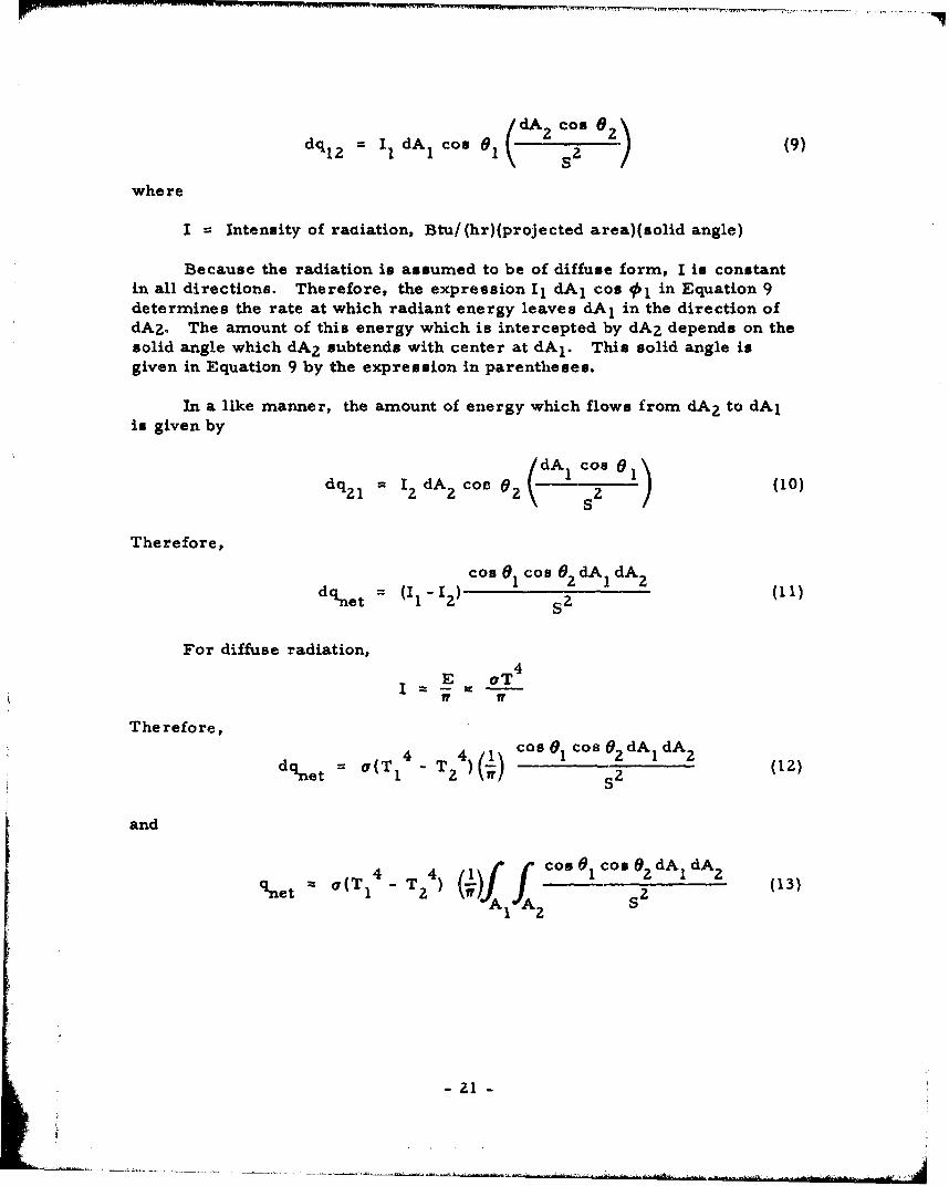
dq I- dAl Co dAo. ( C os ) (9)

where

I Intensity of racdiation, Btu/(hr)(projected area)(solid angle)

Because the radiation is assumed to be of diffuse form, I is constantin all directions. Therefore, the expression Il dAI cos jI in Equation 9determines the rate at which radiant energy leaves dA1 in the direction ofdAz. The amount of this energy which is intercepted by dA 2 depends on thesolid angle which dA2 subtends with center at dAI. This solid angle isgiven in Equation 9 by the expression in parentheses.

In a llke manner, the amount of energy which flows from dA2 to dAlis given by

dq2 I = I2 dAz coo (dAI coo 01) (10)

Therefore,

cos 01 coso 02dA dA2dqnet = (II )2 (11)

For diffuse radiation,E &T 4

Therefore,4 cos0Icos0 2 dA dA

dqt a c(T 1 T T2 ( 2 (12)S

and

4 4 I1 f co C 691 como0 dA IdAqnet (TI4-T 2 4) ')A1 2 (13)A 2 S )

22

b - 21 -

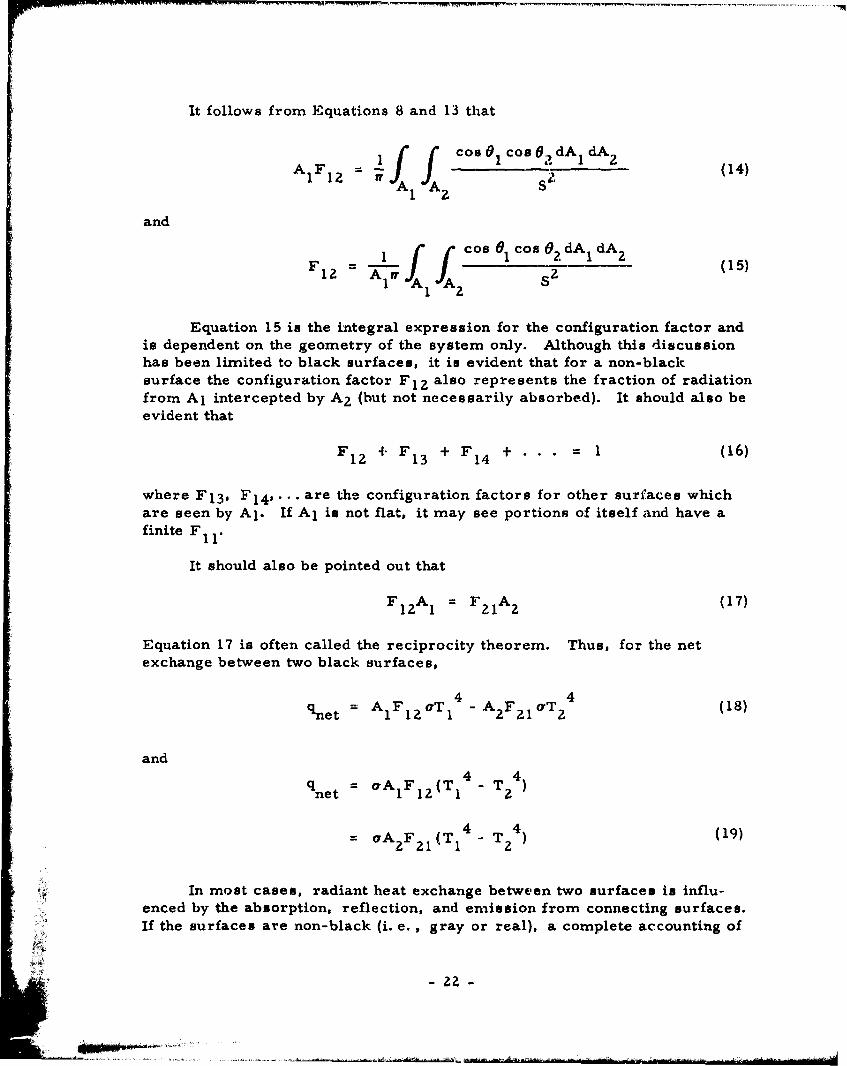
It follows from Equations 8 and 13 that

coo cos 2 dA dA2

A1A IA1" (14)1 Z

and

Cos 6 cois6cs 2dA dA2

F1 2 - ?SA A2 1 (15)

Equation 15 is the integral expression for the configuration factor andis dependent on the geometry of the system only. Although this discussionhas been limited to black surfaces, it is evident that for a non-blacksurface the configuration factor Fl? also represents the fraction of radiationfrom Al intercepted by A2 (but not necessarily absorbed). It should also beevident that

F12 + F13 + F14 += 1 (16)

where F1 3 , F 1 4 ,.... are the configuration factors for other surfaces whichare seen by Al. If A 1 is not flat, it may see portions of itself and have afinite F 1 1.

It should also be pointed out that

F12A, = F 2 1A 2 (17)

Equation 17 is often called the reciprocity theorem. Thus, for the netexchange between two black surfaces,

=AF 4 -AF T24 (18)%net 112F~°T 1 221l

and

qnet = aA 1F 1 2 (T 14 T2

4)

= A2 F 2 1 (TI4. T 2) (19)

In most cases, radiant heat exchange between two surfaces is influ-enced by the absorption, reflection, and emission from connecting surfaces.If the surfaces are non-black (i. e. , gray or real), a complete accounting of

2- 22-

. -~-~

all the irterreflections is quite difficult to accomplish analytically.Fortunately, methods are available for the more complicated radiationproblems. Theme are discussed in Section VI.

23 -

Section IV

THERMAL RADIATION ENVIRONMENT IN SPACE

Incident radiation consists of the direct radiation from the sun,scattered and reflected sun radiation from a nearby planetary body, andradiation directly emitted by the planetary body. The value of irradiancevaries over the surface of a vehicle and depends on the relative positionof the surface with respect to the sun and other planetary bodies.

DIRECT SOLAR RADIATION

The release of energy from the sun produces radiation in many forms.Most of the radiation is thermal, concentrated in the visible and infraredspectrum. The total energy radiated in X-ray and ultraviolet bands is onlya very small portion, measured in thousandths of a percent, of the totalenergy output of the sun.

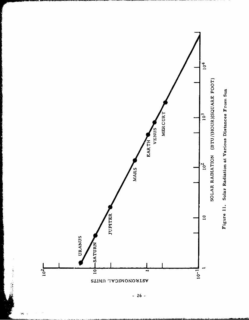
Radiation intensity is inversely proportional to the square of thedistance from the sun. At 1 astronomical unit (the distance from the sun tothe earth), the total value of the solar constant is 443 Btu/(hour)(square foot)(Reference 7). The variation of irradiance for the solar system is shown inFigure 11. The solar constant is influenced by sunspot and other activity,but variations are small (less than 0. 4 percent).

Many calculations are based on the assumption that the sun radiates asa 10, 340 F black body. rhe black body radiant temperature, however, variesfor each wavelength, and these variations should be analyzed for more exactcalculations. Examples of approximate temperatures at which the sunradiates are given in Table I for several wavelengths (Reference 8). Thedeviation in spectral energy distribution from black body radiation isprobably caused by variations in absorption by the solar atmospheric gases.The spectral energy curve of the sun is shown in Figure 12 (Reference 7).

The minimum temperature for any wavelength is approximately6750 F. For the production of very short ultraviolet wavelengths andX-rays, the temperature in the corona is In the range of 1 x 106 F. Sunspottemperatures are approximately 3600 F less than the photosphere; they emitonly about 10 percent as much energy as equal areas of the solar surface.

Curves of intensity and wavelength of the solar spectrum show thatmost of the energy from the sun is carried in wavelengths between 2000 and

2- 5 -

iiiOj!!;PAGEVRE71LjS5- U `WV:I

-44

0 u

a z00

z :>

"-.4

0 0'U

V

o *z

26N -

0.8

0. 7 SOLAR SPECTRAL ENERGY DISTRIBUTIONOUTSIDE EARTH'S ATMOSPHERE

W00.6- BLACK BODY ENERGY DISTRIBUTIONU FOR 10, 340 F

0.5I

0.41

0

_ 0.

0 0.

0.1

00 0.4 0.8 1.2 1.6 2.0 2.4 2.8

WAVELENGTH, U (MICRONS)

Figure 12. Spectral Energy Curve of Sun

- 27 -

=7-

Table 1. Solar Radiation Temperatures

Wavelength Temperature(A) (F)

3500 94302900 94302600 85302200 83602000 76501500 76501200 10,500

20, 000 angstroms, with the maximum energy centered about 4700 angstroms.The approximate energy distribution of solar radiance by percent of thetotal is given in Table 2 for several wavelength intervals (Reference 8).

Table 2. Energy Distribution of Solar Electromagnetic Radiation

ApproximateWavelength Interval Radiant Energy

Type (k) (percent)

X-ray and ultraviolet 1 to 2000 0.2

Ultraviolet 2000 to 3800 7.8Visible 3800 to 7000 41Infrared 7000 to 10, 000 22Infrared 10,000 to 20, 000 23Infrared 20,000 to 100, 000 6

The normal sun produces X-rays with power density on the order of0. 316 Btu/(hour)(square foot). These are probably produced in the corona.During a quiet sun, X-rays reaching the earth are neither very intense norencrgetic. Wavelengths as short as 20 angstroms are present andpenetrate the atmosphere to within 60 miles of the earth's surface when thesun is overhead. During maximum coronal activity the total output of X-raysmay increase by a factor of 2 or 3 and, at the same time, tend to becomeharder with wavelengths as short as 6 or 7 angstroms. Flares are a stillmore important factor in producing hard X-rays, but their intensity nearthe earth is still low.

In the ultraviolet portion of the spectrum below 2000 angstroms, thegreatest portion of the energy is found at the wavelength (1216 angstroms) ofthe resonance emission line of hydrogen atoms. In spectroscopy, this is

. .28

known as the Lyman alpha line. Below the wavelength of Lyman alpha aremany other emission lines. One which appears to have more energy thanthe rest combined, but still much less than Lyman alpha, is found at 304angstroms, which is the wavelength emitted by ionized helium. Theseemissions are detected only above the earth's atmosphere.

The small amount of ozone present in the atmosphere absorbs allwavelengths of ultraviolet radiation below about 2900 angstroms andattenuates those up to 3500 angstroms. Consequently, ultraviolet is muchmore penetrating and intense above approximately 19 miles (100, 000 feet).Above about 47 miles the ultraviolet light is practically unfiltered.

At the infrared end of the spectrum, a number of bands are absorbedin the atmosphere by water vapor and carbon dioxide, but the cutoff wave-length does not occur until in the far infrared. The effect of the absorption,then, is to diminish the intensity but not to eliminate completely the nearinfrared even at the surface.

A thorough discussion of visible and infrared thermal radiation canbe found in Reference 8.

REFLECTED SOLAR RADIATION

The ratio of solar radiation scattered back into space without absorp-tion to that incident upon the planet is termed "albedo". The albedo of anobject is the fraction of the incident energy which is reflected by the objectin the entire band from ultraviolet to the far infrared. The spectralreflectance of an object ideally is the fraction of monochromatic incidentenergy of wavelength X reflected by the object, but in practice it always refersto a finite narrow band. The visual albedo of an object refers only to thevisible part of the spectrum. The luminous reflectance of various objects isshown in Table 3 (Reference 9).

The planetary albedo is caused by scattering at the planet's surface,scattering by clouds and dust in its atmosphere, and molecular scattering byatmospheric gases. The characteristics of the radiation emerging fromthe top of a planetary atmosphere are complex as they are functions ofterrain, cloud covers, optical thickness of the atmospheric gases, the sun'selevation angle, nadir angle, azin. i angle with respect to sun, and radia-tion wavelength. The albedo of th various planets is shown in Table 4(References 10 and 11).

The visual albedo of the earth as determined from earth shine varieswith the seasons from 0. 52 in October to 0. 32 in July, with an average valueof 0. 35. Variations in cloudiness may account for most of the seasonablevariations. Reference 11 reports that albedo of clouds alone is about 0. 5,which is in keeping with maximum seasonal values stated. Taking themeasured visual albedo of the whole earth as 0. 39 (Reference 11), the albedo

2- 9 -

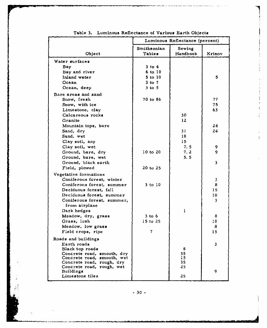
Table 3. Luminous Reflectance of Various Earth Objects

(.Luminous Reflectance (percent)

Smithsonian SewingObject Tables aHandbook Krinov

Water surfacesBay 3 to 4Bay and river 6 to 10Inland water 5 to 10 5Ocean 3 to 7Ocean, deep 3 to 5

Bare areas and sandSnow, fresh 70 to 86 77Snow, with ice 75Limestone, clay 63Calcareous rocks 30Granite 12Mountain tops, bare 24Sand, dry 31 24Sand, wet 18Clay soil, any 15Clay soil, wet 7. 5 9Ground, bare, dry 10 to 20 7. 2 9Ground, bare, wet 5. 5Ground, black earth 3Field, plowed 20 to 25

Vegetative formationsConiferous forest, winter 3Coniferous forest, summer 3 to 10 8Deciduous forest, fall 15Deciduous forest, summer 10Coniferous forest, summer, 3

from airplaneDark hedgesMeadow, dry, grass 3 to 6 8Grass, lush 15 to 25 I0Meadow, low grass 8Field crops, ripe 7 15

Roads and buildingsEarth roads 3Black top roads 8Concrete road, smooth, dry 35Concrete road, smooth, wet 15Concrete road, rough, dry 35Concrete road, rough, wet 25Buildings 9Limestone tiles 25

-30-

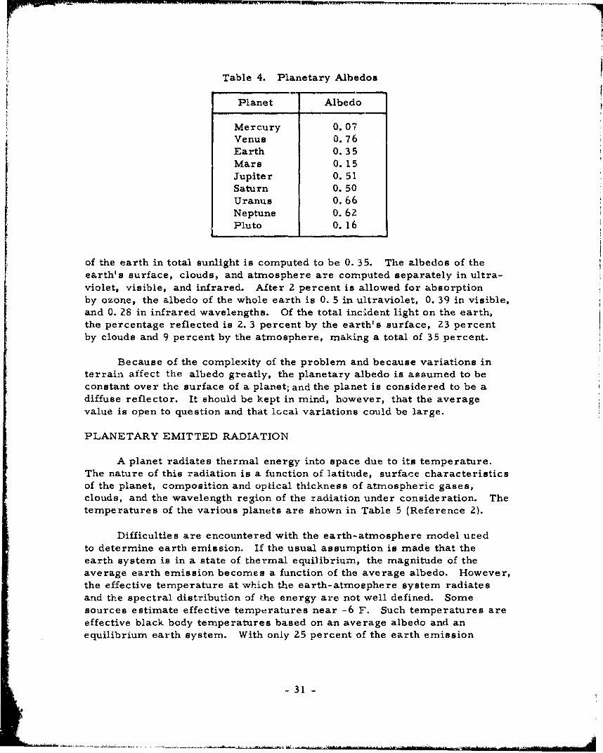
Table 4. Planetary Albedos

Planet Albedo

Mercury 0.07Venus 0.76Earth 0.35Mars 0.15Jupiter 0. 51Saturn 0. 50Uranus 0.66Neptune 0. 62Pluto 0. 16

of the earth in total sunlight is computed to be 0. 35. The albedos of theearth's surface, clouds, and atmosphere are computed separately in ultra-

violet, visible, and infrared. After 2 percent is allowed for absorptionby ozone, the albedo of the whole earth is 0. 5 in ultraviolet, 0. 39 in visible,and 0. 28 in infrared wavelengths. Of the total incident light on the earth,the percentage reflected is 2. 3 percent by the earth's surface, 23 percentby clouds and 9 percent by the atmosphere, making a total of 35 percent.

Because of the complexity of the problem and because variations interrain affect the albedo greatly, the planetary albedo is assumed to beconstant over the surface of a planet; and the planet is considered to be adiffuse reflector. It should be kept in mind, however, that the averagevalue is open to question and that local variations could be large.

PLANETARY EMITTED RADIATION

A planet radiates thermal energy into space due to its temperature.The nature of this radiation is a function of latitude, surface characteristicsof the planet, composition and optical thickness of atmospheric gases,clouds, and the wavelength region of the radiation under consideration. Thetemperatures of the various planets are shown in Table 5 (Reference 2).

Difficulties are encountered with the earth-atmosphere model ucedto determine earth emission. If the usual assumption is made that theearth system is in a state of thermal equilibrium, the magnitude of theaverage earth emission becomes a function of the average albedo. However,the effective temperature at which the earth-atmosphere system radiatesand the spectral distribution of the energy are not well defined. Somesources estimate effective temperatures near -6 F. Such temperatures areeffective black body temperatures based on an average albedo and anequilibrium earth system. With only 25 percent of the earth emission

31 -

Table 5. Planetary Temperatures

Probable TemperaturePlanet (F)

Mercury 339Venus -46Earth -6Mars -68Jupiter -276Saturn -323Uranus -372Neptune ,-400Pluto

coming from the earth and 75 percent coming from the atmosphere, itmight be expected that the spectral energy distribution would be differentfrom that for a black body.

The effective temperature of the earth-atmosphere system is lowenough to cause the bulk of the earth emission to fall in the infrared, wherethe spectral characteristics of many materials are not very sensitive towavelength. Also, the local heat balance of the earth system is too complexto yield useful values for local variations.

- 32 -

Section V

SPACE VEHICLE SURFACE TEMPERATURE ANALYSIS

INTRODUCTION

This section of the report presents some available analytical techniquesand solutions for space vehicle thermal problems. These satellite studiesinclude the following:

1. A simplified steady-state analysis for near-earth orbits based ona cylindrical satellite configuration with its axis on a line passingthrough the center of the earth

2. An IBM 7090 program for the transient heat transfer analysis ofa multi-sided space vehicle in any elliptical or circular orbit

3. A space thermal environment study, including spherical,

cylindrical, hemispherical, and flat- sided satellites

Regardless of the type of temperature control system used aboard aspace vehicle, system requirements are a function of the vehicle's outersurface temperature. These surface temperatures, in turn, are dependent

on the following parameters:

Orbital characteristicsOptical properties of surfaces and components, such

as emittance and absorptanceVehicle orientation to sun and planetHeat capacity of vehicle walls and equipment

Conductive, radiative, and possibly convective heattransfer between surfaces and equipment

Internal heat generationAerodynamic heating for near-earth orbits below 200

miles

Solar constantPlanetary albedoPlanetary emissionVehicle configuration

- 33 -

i: W

It is also true that, by proper selection of optical properties, thesurface temperatures can be controlled to different levels anywhere withina very large range. In optimizing a vehicle design, however, the selectionof the proper control system is made complex because of the many variationsthat can exist in the parameters listed. Variations caused by errors inorbital characteristics, unknowns in the nature of the radiation environment,vehicle stabilization errors which affect orientation, instability of surfacecoatings, and other uncertainties all influence the heat balance on the vehiclethat determines the surface temperature.

Determination of aerodynamic heating in the free-molecular flowregime will not be considered in this report. For low-altitude orbits below200 miles, however, it may be significant in comparison with the magnitudeof the other energy inputs.

The analytical techniques presented in this section illustrate the com-plexity of the problem. They point out ways of determining the form factorbetween the space vehicle and the planet and sun, and the manner in whicheach of the factors enters into the heat balance.

- 34 -

SIMPLIFIED SPACE RADIATION ANALYSIS

The discussion here is of a simplified space radiation analysis whichtakes into account the contributions of solar and terrestrial radiation andassumes steady-state heat transfer. The material was prepared byAiResearch Manufacturing Division for incorporation in this report.

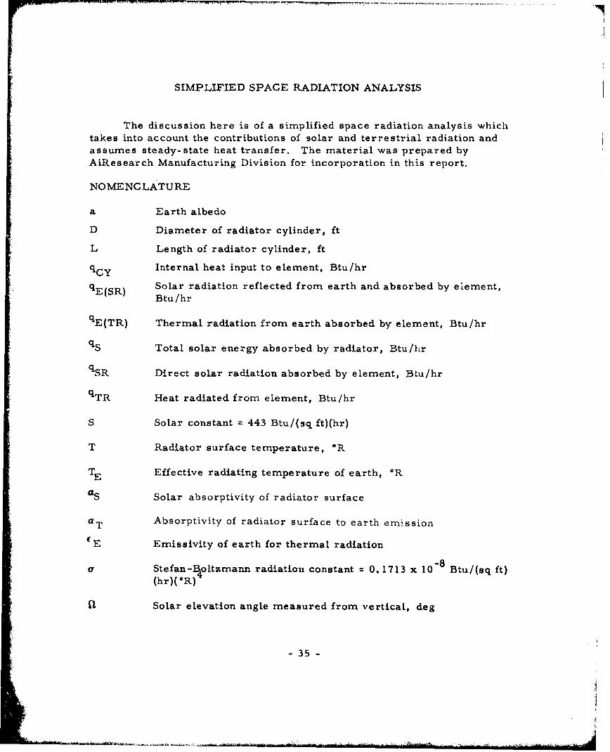
NOMENCLATURE

a Earth albedo

D Diameter of radiator cylinder, ft

L Length of radiator cylinder, ft

qCY Internal heat input to element, Btu/hr

qE(SR) Solar radiation reflected from earth and absorbed by element,Btu/hr

qE(TR) Thermal radiation from earth absorbed by element, Btu/hr

qs Total solar energy absorbed by radiator, Btu/hr

q SR Direct solar radiation absorbed by element, Btu/hr

q TR Heat radiated from element, Btu/hr

S Solar constant = 443 Btu/(sq ft)(hr)

T Radiator surface temperature, °R

TE Effective radiating temperature of earth, °R

aS Solar absorptivity of radiator surface

aT Absorptivity of radiator surface to earth emissionCE Emissivity of earth for thermal radiation

a Stefan-Boltzmann radiation constant = 0. 1713 x 10-8 Btu/(sq ft)(hr)(*R)4

Solar elevation angle measured from vertical, deg

-35-

HEAT BALANCE

The thermodynamic aspects of the heat transfer problem are illus-trated by considering the steady-state heat flow balance equation (heat

outflow equals heat inflow) for an element of surface area

dq+TR = dqCy dqSR + IdqE (T) + dqE(SR) (20)

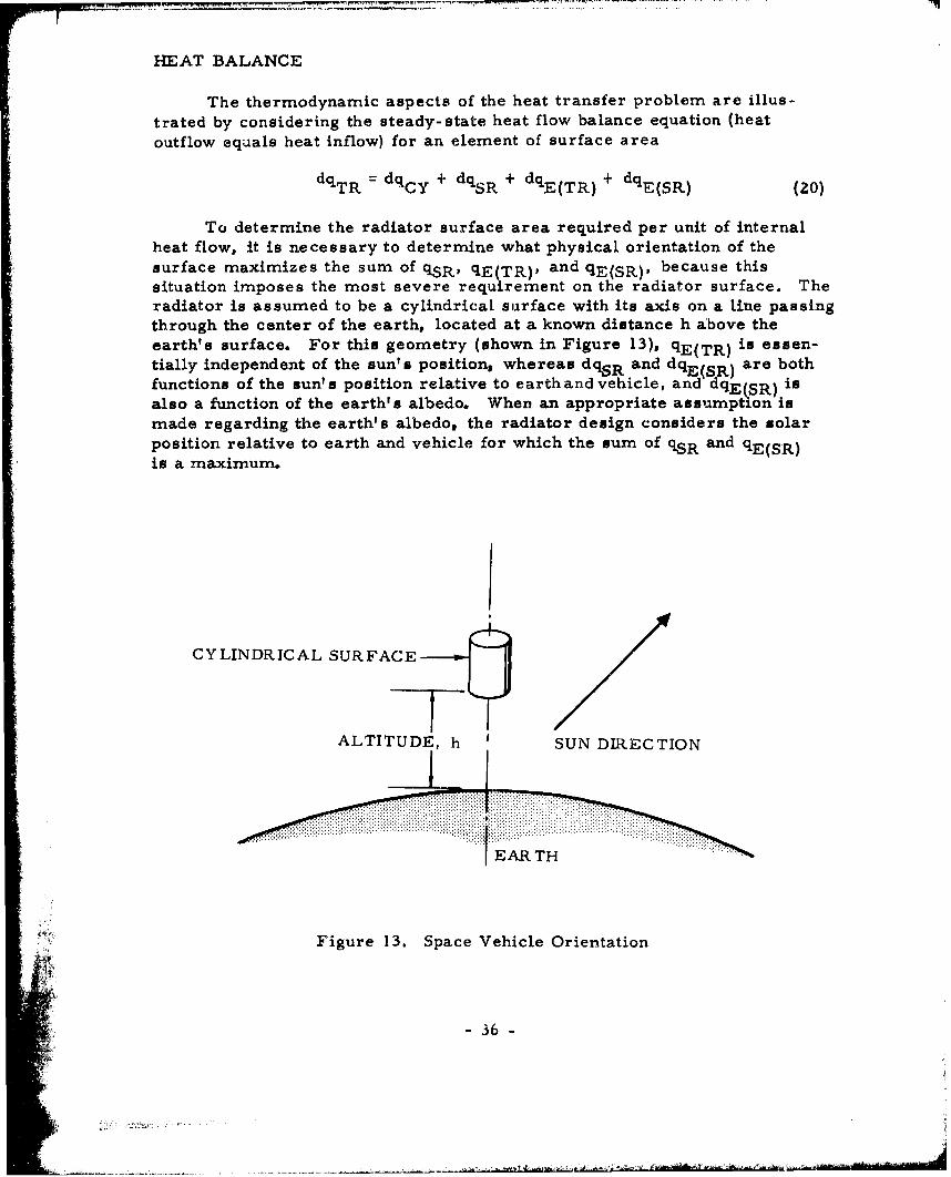
To determine the radiator surface area required per unit of internalheat flow, it is necessary to determine what physical orientation of thesurface maximizes the sum of qSR, qE(TR), and qE(SR), because thissituation imposes the most severe requirement on the radiator surface. Theradiator is assumed to be a cylindrical surface with its axis on a line passingthrough the center of the earth, located at a known distance h above theearth's surface. For this geometry (shown in Figure 13), qE(TR) is essen-tially independent of the sun' s position,0 whereas d%R and dqE(SR) are b .othfunctions of the sun' s position relative to earth and vehicle, and dqE_(SR) isalso a function of the earth's albedo. When an appropriate assumption ismade regarding the earth's albedo, the radiator design considers the solarposition relative to earth and vehicle for which the sum of qSR and qE(SR)is a maximum.

CYLINDRICAL SURFACE

ALTITUDE, h SUN DIRECTION

EARTH S...........

.• Figure 13. Space Vehicle Orientation

-• - 3 6 -

.... .:. .

ANALYSIS DESCRIPTION

In the analysis which follows, the radiator surface required per unitheat flow rate is determined as a function of the radiator surface tempera-ture and a parameter which includes the effects of the values chosen for thevarious emissivities and absorptivities involved and for the earth's albedo.

The analyis was performed in two parts: (1) consideration of asimplified geometry in which the earth is assumed to be an infinite plane,and (2) refinement of the simplified geometric model to take into account thespherical shape of the earth. This approach has an advantage in that thefirst part illustrates the essential physical phenomena, unobscured by theprocedural complications of the second part.

Simplified Geometry Analysis

To determine the solar eleration angle o., at which the sum of qsR andqE(SR) is maximized, the definition is made that

qs = qSR + qE(SR) (21)

The term qs is thus the total solar energy absorbed by the radiator.Defining further,

qSR Sa DLS sinf2 (22)

1I a DLaS cos fl (23)

The factor 1/2 is used in Equation 23 for qE(SR) because the infinite plane is50 percent effective in enclosing the radiator.

To determine the maximum value of qs and the value of 0 at whichthis maximum occurs, dqs/dil is set equal to zero. It follows that

dq - [as cosgl) (24)[ a a S DLS (osinl Qa + o(4

DLS cos - sin(2) (25)

- 37 -

To define the angle ,1 at which the tota? solar radiation absorbed

by the radiator is maximize~a,

=tan- (-1 -) (26)

From which

2

sin 1 = (27)max 4

,a +--Va

and

coso• = (28)max 4

1 22V a

The maximum solar radiation absorbed by the radiator is

2 +eqS(max) aS DLS -ra 2" (29)

4

+ -- I

2 2

aDLS 1I+ -4

The effect of earth albedo a on'lmax and qs(max) is shown in the followingtable:

Solar Elevation S(max)Earth Albedo Angle Umax

a (deg) aS DIS

0 90 1.000. 2 72. 5 1.050.4 57.9 1. 18

o0.6 46.7 1.370. 8 38. 5 1.611. O• 28.3 1.86

-38-

For a small element of radiator surface, dA, the heat balanceequation is

dqTR = dqcY + dqE(TR) + dqS(max) (30)

From which can be obtained

4 41AISýA\aOT4A = qCY + ETTE4 :L+aS )VI + 1 4 (31)

Refined Geometry Analysis

Refinement of the previous analysis, to account for a spherical earthrather than an infinite plane, is desirable because the simplified analysismay be conservative to an unrealistic degree.

The analytical process to be followed is similar in principle to thatdiscussed previously. In the present analysis, expressions for qE(SR) and

,E(TR) contain shape factors in the form of integrals which must beevaluated numerically. Because the mechanics of the derivations are quitecumbersome, only the results of each analysis are reported in the followingdiscussion.

Evaluation of qE(TR)

Evaluation of qE(TR), assuming a spherical earth of 39 6 0-mile radiusand a radiator altitude of approximately 300 miles above the earth's surface,leads to the result

qE(TR)2 = 0.2722 E a T A 4 (32)

which compares with the previous result given by Equation 31

qE(TR)1 = • E aT TE (33)

Equation 33 was calculated assuming the earth to be an infinite plane. Thisresult indicates that the radiator surface absorbs only 54. 4 percent of thethermal radiation from the earth as estimated previously.

- 39 -

Evaluation of qE(SR)

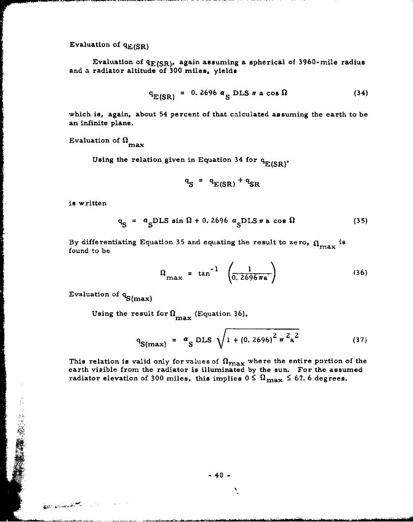
Evaluation of qE(SR), again assuming a spherical of 39 6 0-mile radiusand a radiator altitude of 300 miles, yields

= 0. 2696 a DLS n a cosol (34)

which is, again, about 54 percent of that calculated assuming the earth to bean infinite plane.

Evaluation of &mmax

Using the relation given in Equation 34 for qE(SR)'

q = qE(SR) + qSR

is written

qs = asDLS sin Q + 0. 2696 a sDLSira cos (35)

By differentiating Equation 35 and equating the result to zero, m isfound to be

a = tan- ((6 1 (36)max .2696yra

Evaluation of qs(max)

Using the result for ma (Equation 36),max

S(max) = a LS ýI + (0. 2696) i a

This relation is valid only for values of fmax where the entire portion of theearth visible from the radiator is illuminated by the sun. For the assumedradiator elevation of 300 miles, this implies 0 • •max • 67. 6 degrees.

-40

' -. -

IBM 7090 PROGRAM FOR TRANSIENT HEAT TRANSFER ANALYSISOF ORBITING SPACE VEHICLES

An IBM 7090 program has been developed at S&ID which will simulatethe thermal environment of a multisided space vehicle in any earth orbit.This program will determine the transient temperature history of thesatellite shell; and, if desired, will also provide the complete history ofthe radiant energy incident upon the vehicle surfaces due to direct solarradiation, earth emission, and earth reflected solar radiation. Theseheat loads can be used as input data in a general heat transfer program ifit is desired to obtain a detailed thermal analysis of the interior of thevehicle.

The evaluation studies presented in Section VIII were obtained throughthe use of this program. They demonstrate the flexibility of the programwhen a parametric study is conducted.

A description of the analysis techniques utilized by the program ispresented in this discussion. The areas covered are orbital mechanics,earth shadow intersection points, vehicle configuration and orientation,temperature determination, and vehicle-to-earth geometric configurationfactors. A complete presentation of these subjects, as well as programingtechniques and program philosophy, can be found in report SID 61-105,"Program for Determining Temperatures of Orbiting Space Vehicles, " byG. A. McCue (Reference 33). Data entry, data output, sample problems,the program listing, and program flow diagram are also contained inreport SID 61-105.

NOMENC LATURE

A Surface area of satellite, sq ft

a Semimajor axis of orbit ellipse

a Semimajor axis of shadow ellipse5

A Angle defined in Figures 27 and 28

b Semiminor axis of orbit ellipse

c Construction defined in Figure 25

41-

_ Cp Specific heat, Btu/(l'b rn) (° R)

d Construction defined in Figure 25

E Eccentric anomaly

EE Planetary emission, Btu/(hr) (sq ft)

e Eccentricity of orbit ellipse

FE Geometric form factor for planetary emission

FR Geometric form factor for reflected solar radiation

Fs Geomatric form factor for direct solar radiation

h Height above earth' s surface

Si Inclination of orbit ellipse

M Mean anomaly

m Subscript indicating mass

P Semilatus rectum of orbit ellipse

P Perigee vector

q Internal heat load, Btu/hr

qo Construction defined in Figure 25

r Radius of spherical vehicle

rE Planetary albedo

0 ro Radius from geocenter (orbit ellipse)

Srs Radius from geocenter (shadow ellipse)

R Earth's radius

RE Reflected solar energy from planet, Btu/(hr) (ftz)

S Solar constant, Btu/(hr) (ft2 )

S *o Sun's projection upon the orbit plane

s Construction defined in Figures 27 and 28

t Time, hr

T Temperature, R

=To Epoch time

S .... -4

Tm Maximum expected temperature, OR

Ts Fraction of orbit time in earth's shadow

V Velocity

W Mass of satellite or surface, lbm

x, y, z Rectangular coordinates of equatorial coordinate system

a Construction defined in Figures 26 through 28

as Solar absorptivity of satellite or surface

aE Infrared absorptivity of satellite or surface

aR Absorptivity to reflected solar

Angle between S--0 and P vectors

Y Construction defined in Figures 26 through 28

Construction defined in Figures 27 and 28

Construction defined in Figures 27 and 28

es Emissivity of satellite surface

'1 Construction defined in Figures 27 and 28

0 True anomaly increment between satellite's position and the lineof nodes

c-a True anomaly

Angle between earth-sun line and the vertical between the earthand satellite

ON Angle between the normal to a satellite surface and the linebetween the sun and satellite

01 Angle between the normal to a satellite surface and the line

between the earth and satellite

02 Half of the angle subtended by the earth as viewed from the

satellite

P Gravitation constant

Cr Stefan-Boltzmann constant = 0. 1713 x 10-8

Btu/(hr) (sq ft) (OR 4 )

010 Mean anomaly at epoch

-43-

56 Angle betwe#:n the satellite and the sun's projection upon the

orbit plane

91c Angle defined in Figures 27 and 28

co Argument of perigee

Right ascension of the ascending node

ORBITAL MECHANICS

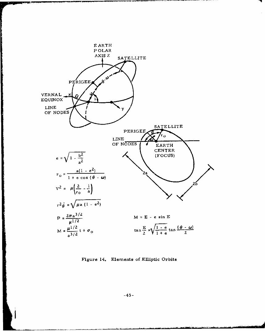
The physical model of orbital motion to be utilized in this analysis isan isolated dynamic system consisting of an earth, an earth satellite, and asun which revolves in the ecliptic ir. the astronomical place of the apparentsun, but is infinitely distant from earth. It is assumed that the earth hasno atmosphere, and is represented gravitationally by the zero-order andsecond-order spherical harmonics of its potential. It is further assumedthat such a trajectory can be described as a function of time by consideringa set of six varying orbital elements. The elements which will be used forthiL analysis are semimajor axis, eccentricity, argument of perigee, rightascension of the ascending node, inclination, and the mean anomaly at epoch(a, e. (a, Q/, i, a.). These elements, along with pertinent equations ofelliptical motion, are indicated in Figure 14. The position of the satellitein the ellipse is described by the angular advance from perigee, 0 - CU(true anomaly). The presence of harmonics in the earth's gravitational

potential will cause periodic and secular variations in several of the orbitalelements. Only the secular perturbations which result in regression ofthe nodes and advance of the perigee position are considered in thisanalysis. Other periodic changes nave negligible effect upon the shadowintersection problem. First-order pertu.rbation theory as developed byCunningham (Reference 4) has been applied to determine these variations.

The angles 0 and wo are then described as a function of time by thelinearized expressions

0 + 0 (t - TO) (38)

(a =ao0 + a(t - TO) (39)

where 6 and L are obtained from Cunningham's equations, and t - To is thetime since epoch.

The geocentric position of the sun is computed by the program fromlinearized expressions involving the earth's mean motion and the equation oftime as a function of date. A simple transformation of coordinates can then

-44-

-22- .

EARTHP OLARAXIS zAXSZ SATE LLITE

VERNALEQUINOX

LINELN

OF NODES 1 EARTHCENTER

e= 1FOCUS)

•i ~ ~a( I - ez). /

V2_2ro = pa(l e2)

rz• %•aI ez)

p = 27'a 3 /Z M = E e sin EIE1/zE tan

M=0a/- t+ Oro tan-1VT-etna3 /2 22

Figure 14. Elements of Elliptic Orbits

-45-

be employed to yield the sun's position relative to an orbit plane coordinatesystem. (It should be noted that a more detailed description of the orbitalmechanics and associated vector algebra can be found in Reference 33.)

SOLUTION FOR SHADOW INTERSECTION POINTS

Perhaps the most important factor that contributes to temperaturevariations during any orbital revolution is the satellite's being eclipsed bythe earth's shadow. For this reason it is important to accuraLely incorporatethis effect into any temperature prediction program.

A method for determining the shadow entrance and exit true anomaliesfrom the coordinates of the sun relative to the orbit plane system was devisedand packaged as a Fortran subroutine for the IBM 7090. Further informationabout this subroutine and its use in computing the percent of eclipse time asa function of various orbit parameters may be found in Reference 13. Abrief description of the calculation scheme employed by this subroutineappears below.

The relative orientation of the orbit, earth, and sun having beenspecified, it is seen that the earth casts a shadow which will at timeF eclipsethe satellite. In reality the sun is not at infinity, and casts a convergingconical umbral shadow. However, a rigorous specification of the positionat which the satellite enters and exits from earth's true shadow leads toneedlessly complicated expressions. For this reason, the followingsimplifying assumptions concerning shadow geometry were made:

1. The earth was assumed spherica! with its radius R equa! to 3960statute miles.

2. The earth's shadow was assumed cylindrical and umbral (sun atinfinity).

3. Atmospheric refraction and penumbral effects were neglected.

The soundness of these assumptions was verified through telescopicobservation of satellites as they entered the earth's shadow. Actual entrancetimes observed daring several transits of 1959 Alpha II and 1960 Iota Iusually differed from predictions by only a few seconds.

The points of intersection of an elliptical orbit and a cylinder axiallyoriented toward the sun are the required solution to the stated problem.Describing these positions in three-dimensional notation results in rathercomplicated expressions. Considerable simplification can be achieved byconsidering the projection of the cylindrical shadow upon the orbit plane.(See Figure 15.)

-46-

So(SUN'S PROJECTION)

SI EXTRANEOUS21 SOLUTIONS

3 SHADOW ENTRANCE4 SHADOW EXIT

S•EARTH

• • P

SHADOWELLIPSE3\

Figure 15. Shadow Geometry (Projection Upon Orbital Plane)

-47-

A geocentric ellipse results from the shadow cylinderls cutting theorbit plane, and is described in polar coordinates by

ar (40)a (l -a 2 ) cos2 ' +a(

where r. and a. are in earth radii.

The elliptical orbit can be represented in polar coordinates by

a(l - e2)0 + e cos"T+ (41)

where r and a are in earth radii.0

It is apparent from the geometry of Figure 15 that the two ellipsesneed not intersect; they may be tangent or may intersect in as many as fourpoints. Of course, no more than two of these intersections can representthe required sunlight-shadow transitions, and the remaining solutions mustbe eliminated.

The required solutions must satisfy the condition

Ar =r - r = 0 (42)

A similar expression,

2 2 2(Ar)= r - r = 0 (43)

was incorporated into the subroutine since it yielded less complex equations.A functional iteration scheme was employed to seek the necessary solutionsto the problem.

The fraction of orbit time T spent in the earth's shadow can becomputed by the equations of Figure 14 through introduction of the eccentricanomaly E and the use of Kepler's equation. Thus,

To = [(E 4 - e sin E 4 ) - (E 3 -- e sin E 3)] (44)

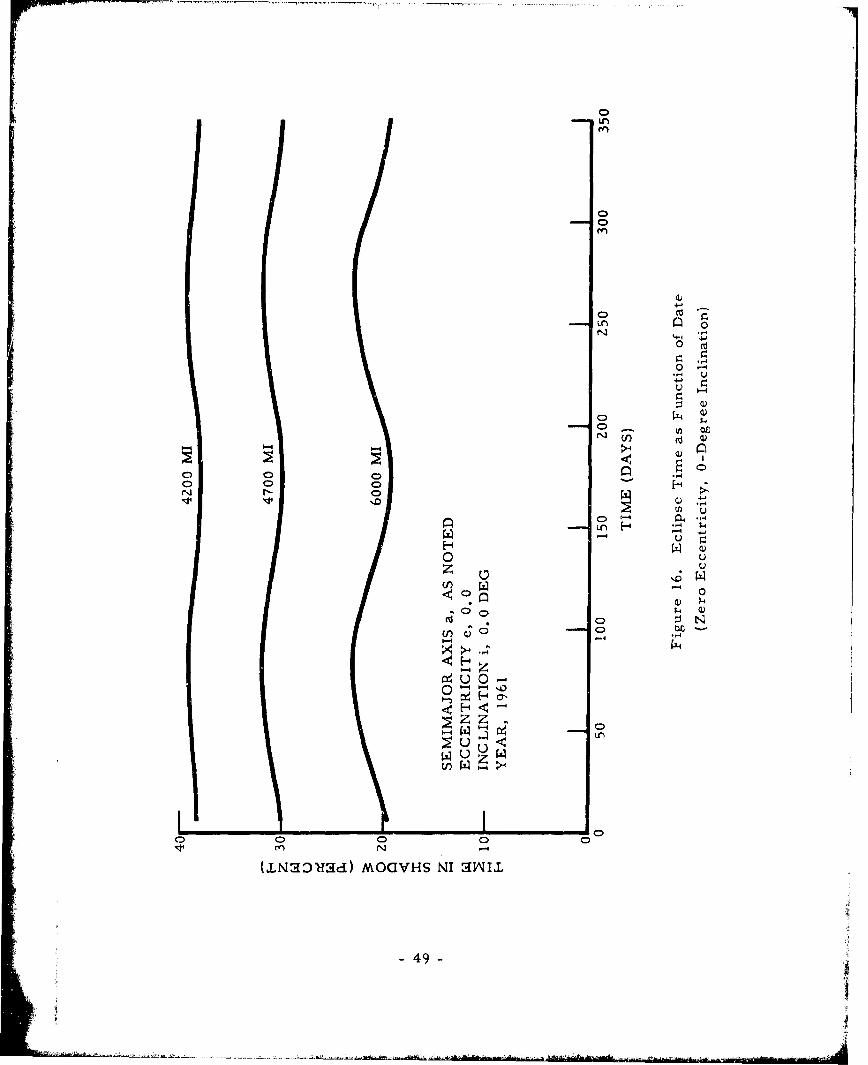
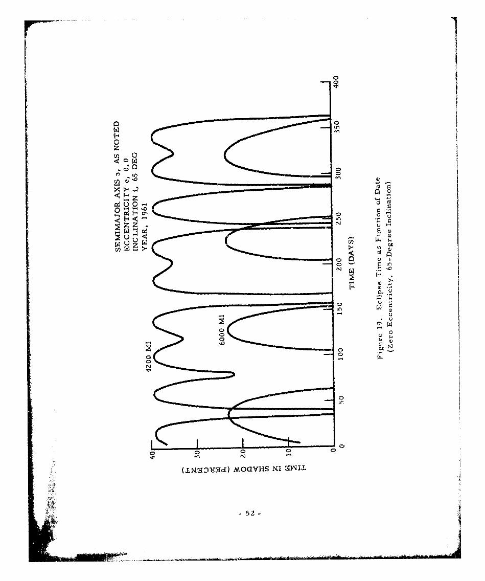
As an illustration of the use of this program, the fraction of each dayspent in the shadow was calculated as a function of date for several parame-ters including inclination, semimajor axis, eccentricity, and launch time.

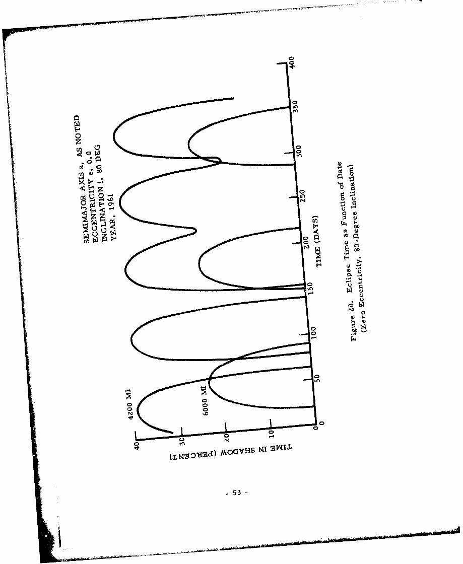
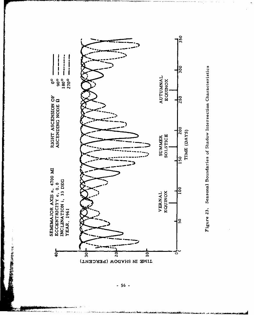
The percent of eclipse time for various orbit classes was computedfrom Equation 44. and is presented in Figures 16 through 23 as a function of

L date. Except as otherwise noted, the initial conditions were as follows:

-48-

LA

M

'4-4

0 ~ cz

0 -4

-4 4-

40

H u uo u

0 0

-4 (.-4

U 00 0 0 0 0

c-

(IMqaD-93) MAOGVHS NI SY4II

-49-

00

P.4 %0

~U0

0 c

C)I

0C 0

05

00

z

~0

C4 u 0

0

(1N1i9T~c1)M~OVHS I j~I.

- -Z. ~

0z(n 0

4-'

04 2 0-' 4-0

00

1:4 E-4 0-

U Z >4z

N --

(JLt~a:)W9d) A&OcVHS NI aV~INIL

-52-

00C4U i

14d

.,A

044ý

- 53 -

I0

LU)

4.)

4.4

000

U)40 4

'41-.4

00

1 -4 '4

C4 00

zU

z 14

543

00

N

00

z0

4-aUl

0 400 4)

0zeU,

0n4

uz o

o 00 4)

u,

5.5-

o i

En".4

000010000

in u

z 4)

uz

~4-4rn 0 0

-4-

od 00 c

Z -Z

"a~

I4)

eno(.LN :)dal) ALOGV S NI3tI

56-

e= 0.0C) = 0.0

= 0.0

T 0 1 January 1961

The results are generally self-explanatory and, therefore, 'only a few of themore interesting points are mentioned here.

Figures 16 through Z0 illustrate the effects of varying the semimajoraxis and/or inclination. With zero inclination (Figure 16), eclipse time isseen to vary seasonally as the sun moves between the northern and southernhemisphere. Increasing the semimajor axis results in increased seasonalvariations, although maximum eclipse time is decreased. Changes inprecession rates that arise from variations in semimajor axis and inclinationare illustrated by Figures 17 through 20. It is to be noted that increasing theinclination and/or the semimajor axis generally yields less eclipse time.

Figure 21 is concerned with variations in eccentricity. The maxima,which occur each time the sun is in the orbit plane, are not always equal aswas the case for circular orbits. Also, increasing the eccentricity tendsto decrease the probability of obtaining total sunlight because the perigeeremains nearer the earth.

Initial right ascension of the ascending node was assigned four differentvalues to produce the curves of Figure 22. This variable, which is a functionof launch time and date, is seen to cause a phase shift in the occurrence oimaxima and minima. Thus, within limits, the launch time can be chosen toproduce the most desirable eclipse conditions.

Figure 23 superimposes the curves of Figure ZZ to illustrate seasonaleffects upon eclipse characteristics. It will be noted that at the equinoxes,when the sun is near the earth's equatorial plane, there is only a slight day-to-day variation in eclipse time. Conversely, at the solstices, the minimabecome quite pronounced.

VEHICLE CONFIGURATION AND ORIENTATION

No attempt was made to write a completely general program withrespect to satellite shape. Thus it was decided that the problem of specifyingvehicle configuration and subsequently orienting the vehicle in space would behandled by a separate subroutine within the program. This requires a newsubroutine for each vehicle configuration, but the extra cost for theirwriting can be amortized through less complex programs, increasedreliability, and better problem understanding.

-57-

At the present time, subroutines arc available for handling the satelliteshapes shown in Figure 24; these are explained in detail in the sampleproblem section of Reference 33. It is ftlt that an experienced Fortranprogramer should be able to devise subroutines for different configurationsas the need arises.

The iniormation determined by the orientation subroutine is utilizedin turn by the geometric form factor subroutine which calculates thegeometric form factors necessary in the temperature analysis. Thegeometric form factor subroutine is described in the next discussion.

GEOMETRIC CONFIGURATION FACTORS

In order to calculate the temperature of an orbiting space vehicle, itis necessary to determine the geometric form factors, which alwaysconstitute a basic problem with radiation heat transfer analysis. Asexplained in the previous discussion, an orientation subroutine suppliesinformation relative to the position of the vehicle with respect to space,the earth, and the sun. This information, in turn, is used by a geometricform factor subroutine which calculates the form factors needed in theanalysis.

Since the form factor subroutine is a separate closed subroutinewithin the main program, it n'ay easily be replaced or changed to incorporatewhatever method of form factor computation is desired. Several routinesthat have beeni devised to compute the form factors for rotating spheres,plane surfaces, and rotating cylindrical surfaces are described here.Listings of the three subroutines for these cases appear in Reference 33.

Rotating Sphere

The direct solar form factor for a uniformly rotating sphere isderived thusly

F Projected areas Total surfdzce area

2Wr 0.25 (45)

4 wr

The geometric form factor for earth emission FE may be derived byconsidering the satellite to be a point source in space viewing the earth.This assumption is correct if the satellite is rotating or has a uniformsurface temperature. Referring to Figure 25, it is seen that FE istherefore equal to the shaded percentage of the sphere with radius c.

-58-

ROTATING SPHERE AXIS INERTIALLY ORIENTEDAXIS ORIENTED TOWARD EARTH

AXIS EARTH ORIENTED VERTICAL ROTATINGAPPROXIMATE CYLINDER(MULTIPLE FLAT SURFACES)

Figure 24. Satellite Configurations Used inTransient Temperature Analysis

-59-

//-•SATELLITE

R EARTH

Figure 25, Planetary Emission Form Factor (Rotating Sphere)

-60-

Considering the right triangle formed by R, cr and (R +,h), one. maywrite

c 2 (h + R) R

c = -h + 5R) (46)

Considering the auxiliary constructions which yield d and q, andcomparing the similar right triangles, it is seen that

d cc R+h

and therefore,

2d = C

R+h

and

qo =c - d =c( (47)

FE is computed by comparing the area of spherical segment withheight q. to the sphere's total surface area. Thus,

Zwrcq -R+

4E 41rc 2 2c

or

F -1- + Z R) (48)FE 2 R+h )Form factors for reflected solar were approximated by the equation

FR - FE cos 0( a49)

This simplification results in an error due to the reflected solar being setequal to zero at the terminator. Actually, the vehicle can still receive somereflected solar radiation when beyond the terminator. However, the errorintroduced by this assumption is felt to be negligible.

-61-

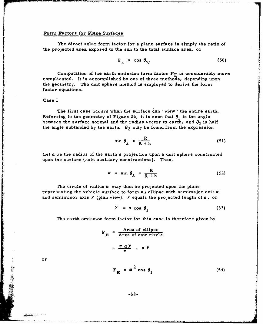
Form Factors for Plane Surfaces

The direct solar form factor for a plane surface is simply the ratio ofthe projected area exposed to the sun to the total surface area, or

F - cos ON (50)

Computation of the earth emission form factor FE is considerably morecomplicated. It is accomplished by one of three methods, depending uponthe geometry. Tha unit sphere method is employed to derive the formfactor equations.

Case I

The first case occurs when the surface can "view" the entire earth.Referring to the geometry of Figure 26, it is seen that 01 is the anglebetween the surface normal and the radius vector to earth, and 02 is halfthe angle subtended by the earth. OZ may be found from the expression

Rsin G2 = R (51)2 R+h

Let a be the radius of the earth's projection upon a unit sphere constructedupon the surface (note auxiliary constructions). Then,

Ra = sinG = R (52)

The circle of radius a may then be projected upon the planerepresenting the vehicle surface to form aa ellipse with semimajor axis aand semiminor axis Y (plan view). Y' equals the projected length of a, or

Y =a cos 01 (53)

The earth emission form factor for this case is therefore given by

Area of ellipseFE Area of unit circle

- a = a

or

F =a 2Cos (54)E

-6?-

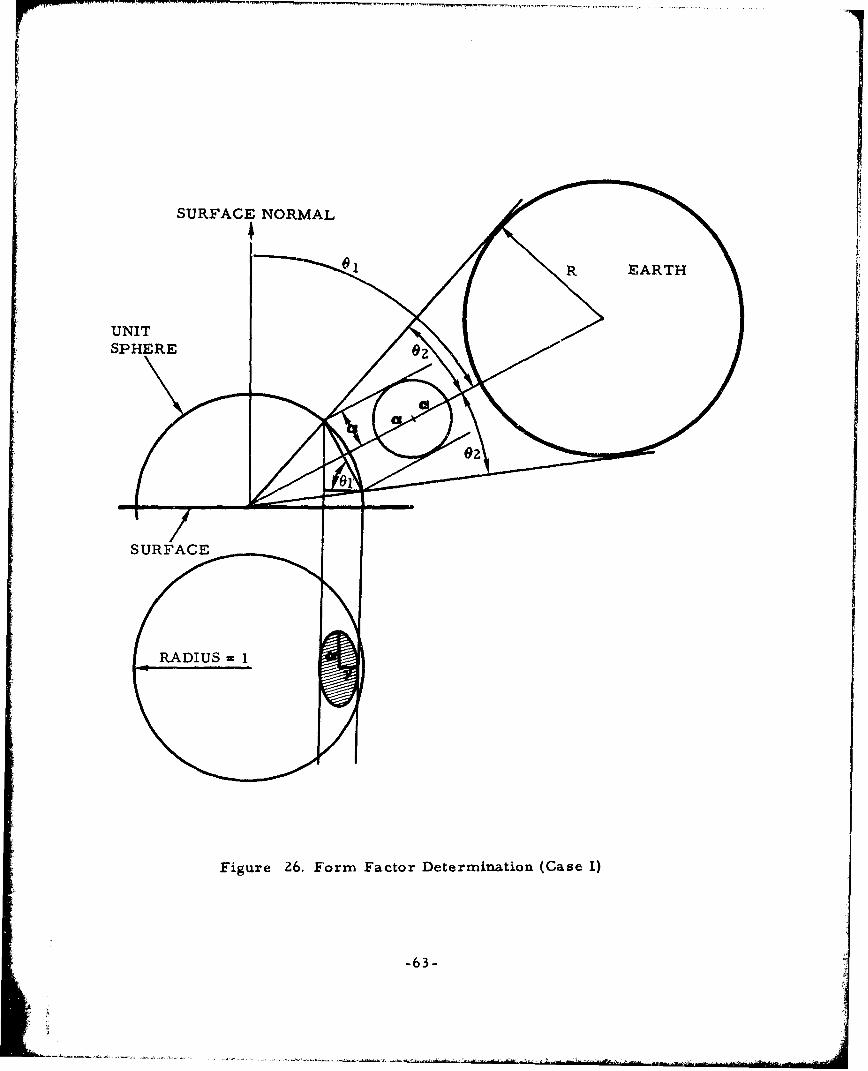
S~ SURFACE NORMAL

Si, EARTH

UNITSPHERE

SURFACE

Figure 26, Form Factor Determination (Case I)

-63-

Case II

When the sum of 01 and 02 exceeds 90 degrees (Figure 27), part of theearth is not visible to the surface. The projection upon the surface of theearth's projection upon a unit sphere forms an ellipse with dimensions aand Y. The areas of interest are the shaded half-ellipse and the similarlyshaded segments of the ellipse and circle. The dimensions 8 and 77. must befound in order to evaluate the area of the ellipse segment. Referring to theauxiliary constructions of Figure 27, the derivation proceeds as follows:

= cos 02

and therefore,

s = C tan (90 -01 cos 0 2 tan (90 -0 1 )

Noting that

cos 01

tan (90 - 01 =ssin 0

and

cos = i- sin = a2

it follows that

- cos 01s a= " Jsin 0

Therefore, 22• Z o 01

1= s cos1 = -a sin 2O (55)

The derivation of 8 proceeds as follows:

8=acos 9 = aVl -sin2.0c

where Cs01

sin 5="=" -aBin 0

-64-

SURFACE NORMAL

UNIT

SPHERE "

SURFACE-

Figure 27. Form Factor Determination (Case 11)

- 65-

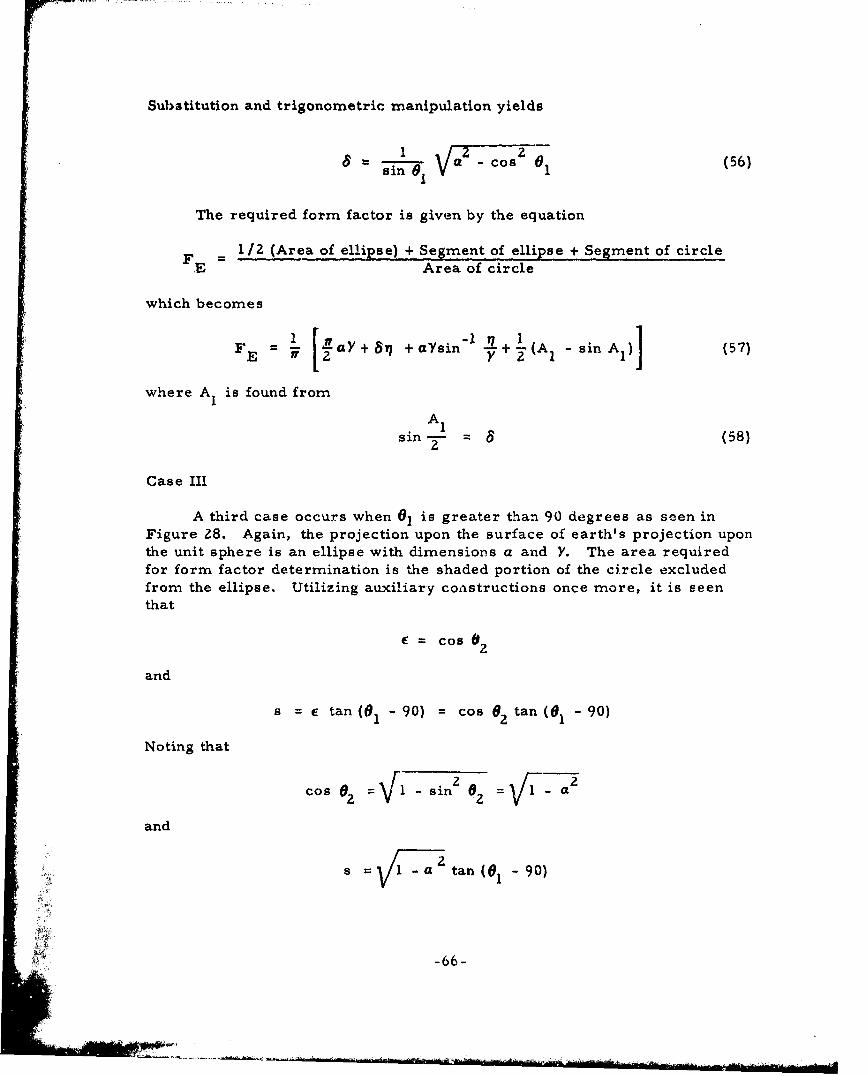
Subatitution and trigonometric manipulation yields

1 -/a 28 in6 1 Va - Cos 1 (56)

The required form factor is given by the equation

FE = 1/2 (Area of ellipse) + Segment of ellipse + Segment of circleArea of circle

which becomes

F -aY+ 8q +aYsin"I + (A sinA (57)E =f 1 2 A

where A is found fromA1

sin- 8 (58)

Case III

A third case occurs when 01 is greater than 90 degrees as seen inFigure 28. Again, the projection upon the surface of earth's projection uponthe unit sphere is an ellipse with dimensions a and Y. The area requiredfor form factor determination is the shaded portion of the circle excludedfrom the ellipse. Utilizing auxiliary constructions once more, it is seenthat

e = cos i2

and

s=c tan (0 1 -90) = cos 06 tan (9I- 90)

Noting that

Cos2 = If- sin 2 OZ = - aZ

and

s 1-a tanl 1 - 90)

-66-

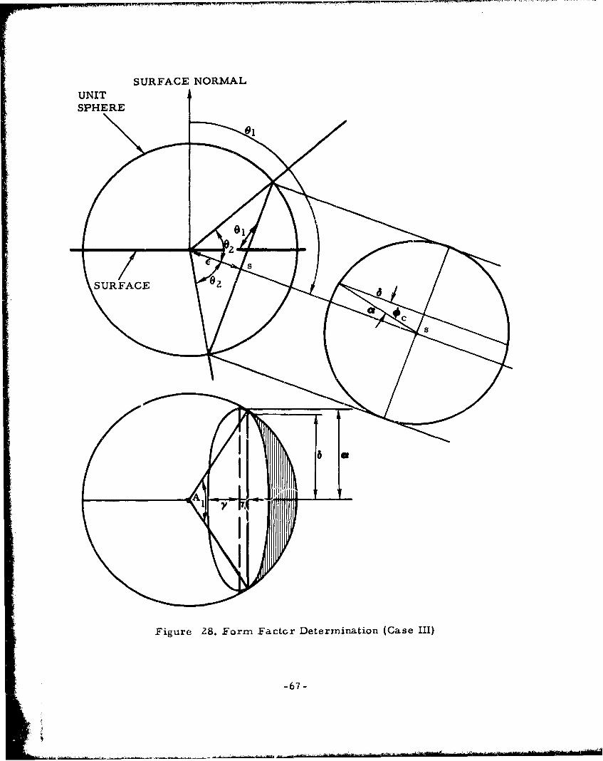
SURFACE NORMALUNITSPHERE

sk

Figure 28. Form Factor Determination (Case III)

-67-

it follows that

i -s cos O1 -'/? oa 0taSS COS a Cos O tan 01- 90) (59)

Smay be derived from the auxiliary construction by first noting that

= acosec = a V/I - sin2 c

where

S Isin •c = 1" V a - tan (01 -90)

Substitution and trigonometric manipulation yields

S= 1 /2 .si2cos (01 - 90) a sin (01 - 90) (60)

The earth emission form factor is found from the expression

Segment of circle + Segment of ellipse - 1/2 (Area of ellipse)

E Area of circle

which becomes

FE = 1 [(AI sinAI)+8+7 +aY sin -2 M ay (61)

where A1 is found from

A1

sin- =

By inspection of the geometry of Figure 28, it is apparent that FEbecomes zero when 01 - 02 > 90 degrees.

It was assumed that the reflected solar form factor could beapproximated by the expression

F F cos 0 (62)R E s

The formulas just developed were incorporated into the form factorroutine for plane surfaces which appears in Reference 33.

-68-

Forra Factors for Curved Surfaces

A good approximation to a curved surface may be obtained by dividingit into an adequate number of plane surfaces. This procedure was utilized tosimulate the rotating cylindrical vehicle of sample problem 4 of Reference 33.In this example, the cylindrical surface was approximated by 24 planesurfaces equally spaced around the principal axis. The contributions of eachplane were then averaged to obtain a single form factor for the rotatingcylindrical surface. (The assumption of rapid rotation results in a uniformsurface temperature. )

TEMPERATURE DETERMINATION

The surface temperature of a space vehicle in orbit about the earth isdetermined by the heat balance between the vehicle surface and itsenvironment, which includes the sun, the earth and its atmosphere, andspace which acts as a heat sink (Figure 29). The vehicle receives solarenergy directly from the sun or indirectly (reflected) from the earth and itsatmosphere. Energy emitted by the earth and its atmosphere also contributesmeasurably to this heat balance. (The largely geometrical problem ofdetermining what radiation the vehicle receives from each source atsuccessive positions around the orbit was presented in the previousdiscussion, which described the procedures used in calculating the geometricform factors. )

Other factors which influence this heat balance are the value of thesolar constant, the planetary albedo, and assumptions concerning planetaryemission. The planetary emitted energy was assumed to be uniform overthe earth's surface and approximately equivalent to that of a black body forthe temperatures shown in Table 5. The vehicle's surface absorptivity forthis energy was assumed equivalent to the total hemispherical emissivity ofthe surface at approximately the same temperature.

The rate of change of the temperature of a surface of an orbitingsatellite may be obtained from

Wc - =-aAFS+aEFAE +aRFAR +q-caAT4 (63)p dt s s EE E R R E

where

T = Temperature of shell, °R

t = Time, hr

W = Mass of satellite or surface, lbm

-69-

RADIATIONTO SPACE

DIRECT SOLAR

E;ARTH SL

EMISSION REFLECTED

SSOLR

RADIATION

,• • --- EARTH

Figure 29. Space Vehicle Heat Balance

c = Specific heat, Btu/(lbm) (°R)p

A = Surface area of satellite, sq ft

q Internal heat load, Btu/hr

a= Stefan-Boltzmann constant = 0. 1713 x I0"8 Btu/(hr)(sq ft}(°R4

as= Solar absorptivity of satellite

aE Infrared absorptivity of satellite

aR = Absorptivity to reflected solar

-70-

.......... .. ....

Fs = Geometric form factor for direct solar radiation

FE = Geometric form factor for planetary emission

FR = Geometric form factor for reflected solar radiation

S = Solar constant, Btu/thr)(sq ft)

EE = Planetary emission, Btu/(hr)(sq ft)

RE = Reflected solar energy from planet, Btu/(hr)(sq ft)

Cs = Emissivity of satellite surface

The temperature prediction program incorporates a finite differenceversion of the Equation 63. The following assumptions are made:

as aR

E = s

RE=SrE (64)

1 - r SEE =- 4 S

FR = FE cos Os

walere

r E = Planetary albedo

es = Angle between earth-sun line and vertical from planet to satellite

The program utilizes several tolerances to ensure that the finitedifference method will yield valid results. Steps are taken to ensure that themaximum time interval used during any step in true anomaly will not exceed.LL time tolerance entered as data or one computed from the equation

TOL = (65)

-71-

Computation is begun by providing approximate values of the varioussurface temperatures at perigee. The program will then computetemperatures at successive intervals around the orbit until it has returnedto perigee. Chances are that the approximate value and the newly computedtemperature at perigee will not agree. The program then repeats thecomputation, utilizing the new temperature as an initial value. Thisiteration process is repeated until initial and final temperatures convergeto within an acceptable tolerance.

Thus, the program obtains a transient temperature history during aparticular revolution of the satellite. Figure 30 shows the describedconvergence effect for a case involving a rotating sphere. Computation wasbegun with an initial temperature guess of 100 F. The lower curve showsthe temperature history computed during the first iteration, while the uppercurve represents the results of the third iteration. After three iterations,the initial and final temperatures coincide. This curve therefore representsthe transient temperature history during the revolution in question.

That the lower curve would r-present the temperature history duringthe first orbital revolution of a satellite injected into orbit with an initialtemperature of 100 F is noteworthy. By the third revolution, thetemperature carve would become rather stable. Thereafter, it wouldexperience slight day-to-day changes brought about by orbital precessionarid other factors.

Although the foregoing discussion was confined to temperaturedetermination, it should be noted that the amount of radiant energy that isabsorbed by each satellite surface from the space environment is alsoavailable from the program. This information may be utilized as inputdata in a general heat transfer program if it is desired to obtain a detailedthermal analysis of the interior of the vehicle. This capability of theprogram may prove to be more important than its capability to computesatellite shell temperature histories.

PROGRAM LISTING AND DECK SE'LTJP

Figures 31 and 32 illustrate the general approach used in the programby showing the main program flow diagram and deck setup. It is beyond thescope of this report to go into detail with respect to these diagrams, since

they are primarily of interest to program writers. It is recommended thatReference 33 be consulted for a complete explanation of these areas ofinterest.

iIL -72-

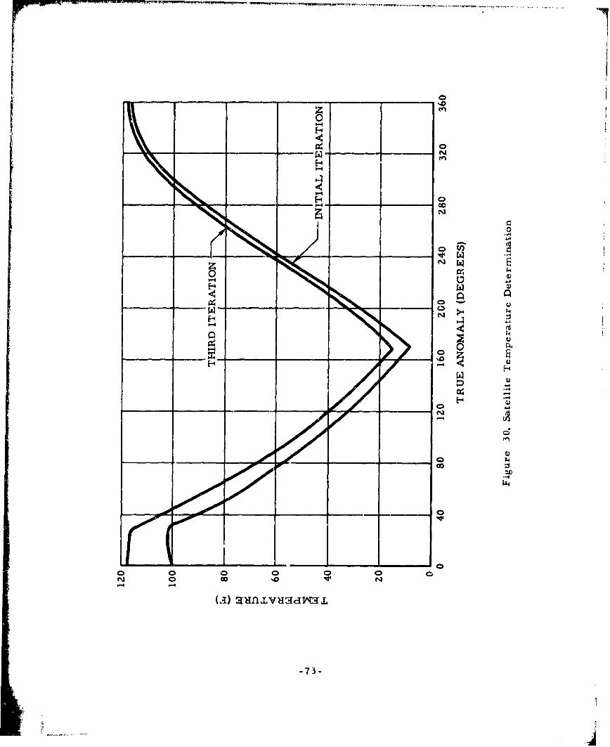
00

%00

-44

0)

000)

N 0N

-73-

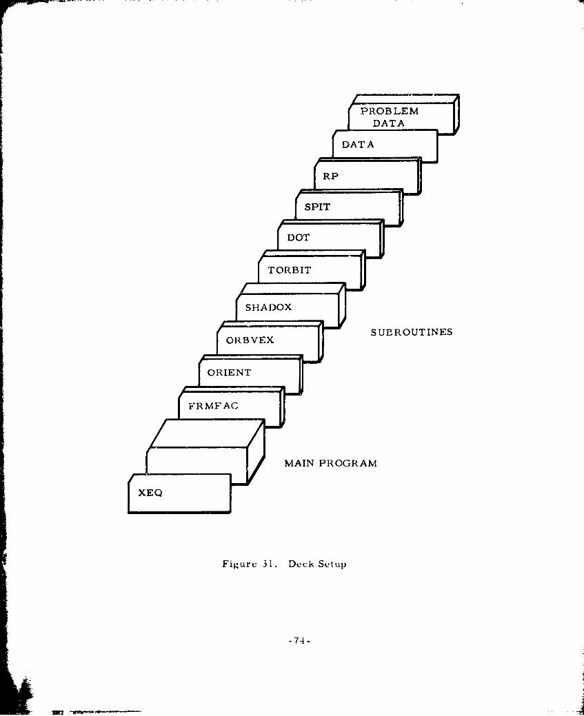
PROBLEMDATA

DATA

SPT

FDOT

SUBROUTINESORBVEX

FRMFAAC

MAIN PROGRAM

XEQ

Figure 31. Deck Setup

-74-

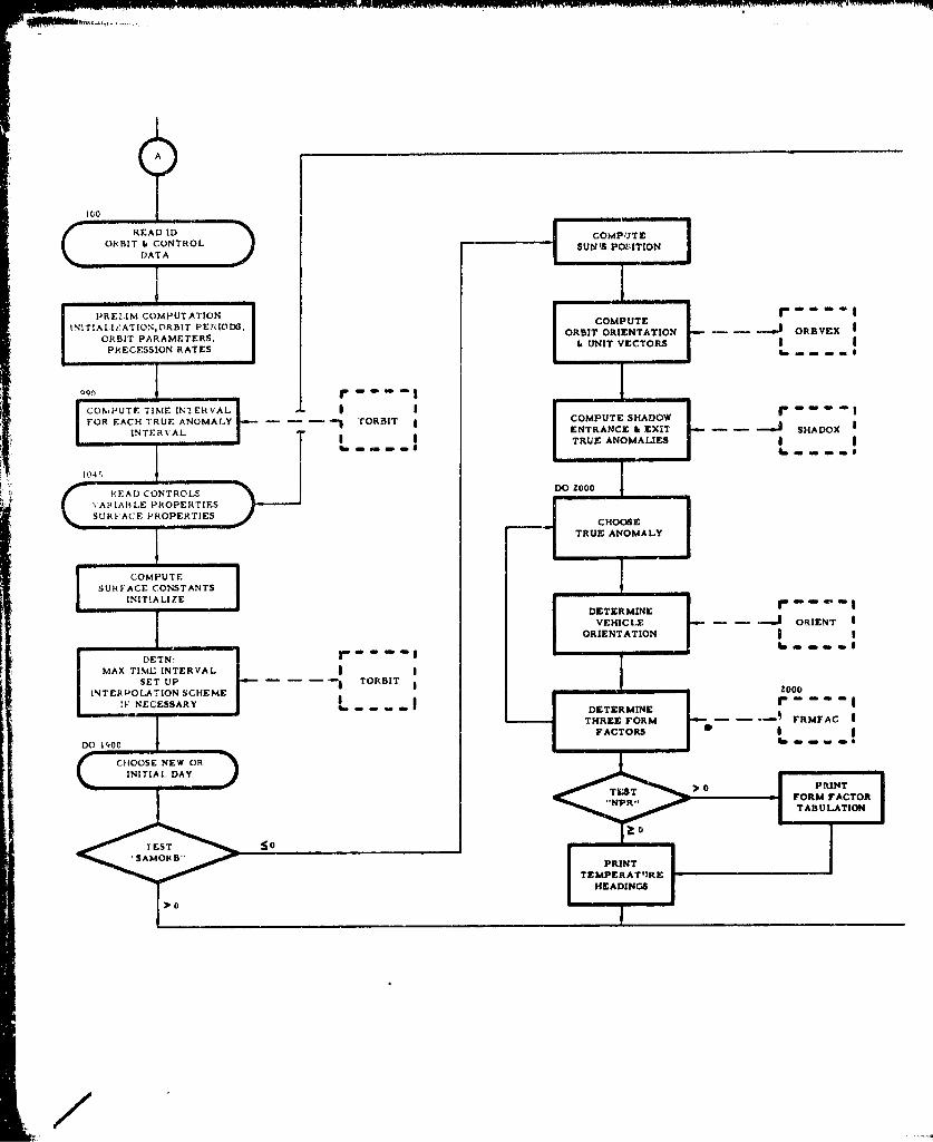
A

1Co

READ IDCOPT

ORBIT , CONTROL SUN'S POSITIONDATA

mlL

PRFL.[M COMPUTATION CO MU r

INITiA L.1 ATION,ORBIT PERIODS, ORBI TE / ORVEX

CRBI'r PARAMETERS, ORBIT ORIENTATION S - - ORB VPRECESSION RATES

COMPUTE TIME IN ERVAL | iFOR EACH TRUE ANOMALY - - - TORBIT COMPUTE SHADOW

ENTRANCE & EXIT - - SHADOX

1 TRUE ANOMALIES

1045

C ,E)AD CONTROLSO

VARIABLE PROPERTIES r C

c SURFACE PROPERTIES I CHOOSE j1 TRUE ANOMALY

COMPUTE

SUR FACE CONSTANTSINITIALIZE/I

DETERMINE rV- -- O IORIENTATION J

OETN- r'MAX TIME INTERVAL I I

SET UP TORBIT ,oo,

INTERPOLATION SCHEME 2000

:F NECESSARY r--DTEMNEs DETERMINE

THREE FORM - - FRMFAC

FACTORS i IDo 1900 11oI

CHOOSE NEW ORINITIAL DAY

TEST >0 PRNT"-- FORM FACTORTABULATION

TESTo"SAMO"S PRINT

TEMPERAT'IREHEADINGS

/

CO'MP U-ESUN'S POSiVION

z ACOMPUTE

oRBIT ORIENTrATION ORBVEX o ! (READ NEW DATA)

F, UNIT VECTORS

>0 TEST DO .3ZO

SAOI INTERPOI

EH r ANCE 4 OLXIT - SlHADOX

A T

TRUJEANOMAL•IES I -I - I~

"C ASP V A RCIM0000

CH O F1900

TRUE ANOMALIES O N N,

CONVERT h

r PRINT EXTERNAL

DETERMINE HEAT LOADSVEHICLE [ - ORIENT DO 31ZS(-CW!IEN rATIO N I

> | 0 i ) 1:

16 - ~<0 op

L,• I• < 01COMPI

ENNEW INI

TEST TEMPERA

DETERMINESTHREE FORM FMFAC CO

FACTORS SICUJ - -E,-TUE ITERATI

-P M

C

TLs r >0 PRINT CONT11

N4R ~TABULATIINPR- :TIOTIREF

33

?! (P 1201

PRINT

ENIFEOATU'NHEADINGS

-J Figure 32.

COMPUT

INUT TO EACH-

ENTRNTMP7,NATUR

ITERTIT LOADS

TTESTN

Do 00

ESLEORRUE ANOAL

Figure~~~

~ ~ T

32 Ma n P o r l w D a rM

o~~~ ~ ~ ~ 75 76 (RA-E AA E

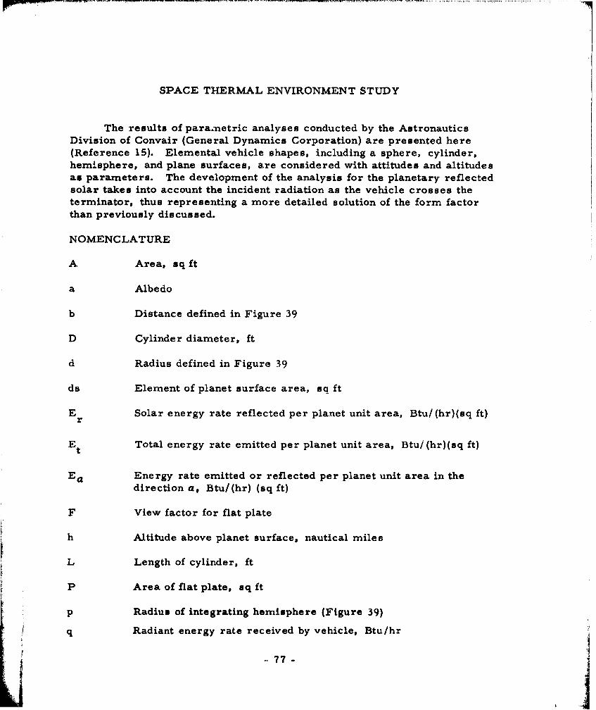
SPACE THERMAL ENVIRONMENT STUDY

The results of paranetric analyses conducted by the AstronauticsDivision of Convair (General Dynamics Corporation) are presented here(Reference 15). Elemental vehicle shapes, including a sphere, cylinder,hemisphere, and plane surfaces, are considered with attitudes and altitudesas parameters. The development of the analysis for the planetary reflectedsolar takes into account the incident radiation as the vehicle crosses theterminator, thus representing a more detailed solution of the form factorthan previously discussed.

NOMENCLATURE

A Area, sq ft

a Albedo

b Distance defined in Figure 39

D Cylinder diameter, ft

d Radius defined in Figure 39

ds Element of planet surface area, sq ft

"E Solar energy rate reflected per planet unit area, Btu/ (hr)(sq ft)r

"Et Total energy rate emitted per planet unit area, Btu/ (hr)(sq ft)

Ea Energy rate emitted or reflected per planet unit area in thedirection a, Btu/(hr) (sq ft)

F View factor for flat plate

h Altitude above planet surface, nautical miles

L Length of cylinder, ft

P Area of flat plate, sq ft

p Radius of integrating hemisphere (Figure 39)

q Radiant energy rate received by vehicle, Btu/hr

-77-

R Radius of planet, nautical miles

r Radius of sphere or hemisphere, ft

S Solar constant, Btu/(hr)(sq ft)

x Distance defined in Figure 39 or Figure 42

a Angle between normal to planetary element and vector tovehicle, deg

Angle between earth-sun vector and extended normal to planetaryelemental area, deg

Y Angle between vertical to vehicle and cylinder or hemisphereaxis or normal to flat plate, deg

Angle between axis of cylinder or hemisphere or normal to flatplate and vector from vehicle to planetary elemental area, deg

Angle between vehicle-earth vector and vector from vehicle t)

planetary elemental area, deg

0 Spherical ordinate, deg

o0 Spherical ordinate of horizon as seen from vehicle, deg

A Angle defised in Figure. 39, deg

p Distance between planet surface element and vehicle, naut mi

05 Spherical abscissa, deg

0c Angle of rotation of axis of cylinder or hemisphere or normal toflat plate about vertical to the vehicle, measured from plane of theearth-vehicle and earth-sun vectors, deg

Angle defined in Figure 39, deg

6 Angle defined in Figure 39, deg

Subscripts

'• 0, 1,O '~ Refer to various intersections on planetary sphere

-78-

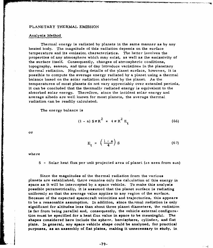
PLANETARY THERMAL EMISSION

Analysis Method

Thermal energy is radiated by planets in the same manner as by anyheated body. The magnitude of this radiation depends on the surfacetemperature and its emission characteristics. The latter involves theproperties of any atmosphere which may exist, as well as the emissivity ofthe surface itself. Consequently, changes of atmospheric conditions,topography, season, and time of day introduce variations in the planetarythermal radiation. Neglecting details of the planet surface, however, it ispossible to compute the average energy radiated by a planet using a thermalbalance based on the solar radiation absorbed by the planet. As thetemperatures of most planets do not vary appreciably over extended periods,it can be concluded that the thermally radiated energy is equivalent to theabsorbed solar energy. Therefore, since the incident solar energy andaverage albedo are well known for most planets, the average thermalradiation can be readily calculated.

The energy balance is

( -a) SiR2 4nR Et (66)

or

E t 4 ( ) S (67)

whe re

S = Solar heat flux per unit projected area of planet (as seen from sun)

Since the magnitudes of the thermal radiation from the variousplanets are established, there remains only the calculation of this energy inspace as it will be intercepted by a space vehicle. To make this analysispossible parametrically, it is assumed that the planet fiurface is radiatinguniformly so that the average value applies to any region of the surface.Because of the expected spacecraft velocities and trajectories, this appearsto be a reasonable assumption. In addition, since thirmal radiation is onlysignificant for altitudes less than about three planet diameters, the radiationis far from being parallel and, consequently, the vehicle external configura-tion must be specified for a heat flux value in space to be meaningful. Theshapes considered here include the sphere, hemisphere, cylinder, and flatplate. In general, any space vehicle shape could be analyzed, for practicalpurposes, as an assembly of flat plates, making it unnecessary to study, in

-79-

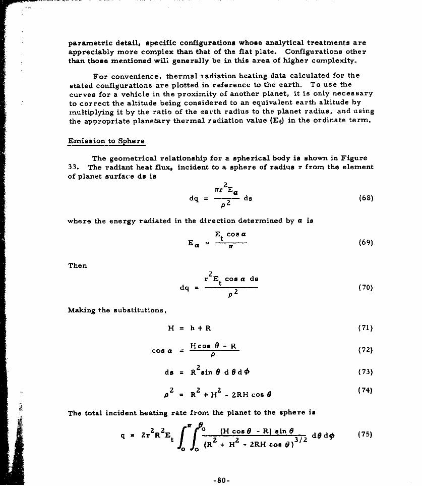
parametric detail, specific configurations whose analytical treatments areappreciably more complex than that of the flat plate. Configurations otherthan those mentioned will generally be in this area of higher complexity.

For convenience, thermal radiation heating data calculated for the

stated configurations are plotted in reference to the earth. To use thecurves for a vehicle in the proximity of another planet, it is only necessaryto correct the altitude being considered to an equivalent earth altitude by

mnultiplying it by the ratio of the earth radius to the planet radius, and using

the appropriate planetary thermal radiation value (Et) in the ordinate term.

Emission to Sphere

The geometrical relationship for a spherical body is shown in Figure33. The radiant heat flux, incident to a sphere of radius r from the elementof planet surface do is

P2

nrZ~

dq = -- ds (68)

where the energy radiated in the direction determined by a is

Ea Et cos aEa'7r (69)

Then

r Et cos a dsdq =2 (70)

p 2

Making the substitutions,

H h+R (71)

Hcos 0 - Rcos a = p(72)

2ds = R sin 0 d0dt (73)

P = R +H - ZRH cos (74)

The total incident heating rate from the planet to the sphere is

i q = ZrREt 0 (H cos0 - R)sin dsdi (75)R2 + H2 - 2RH cos 0)3/2

-80-

SPHERICAL BODY

h

iP

ds 0

RPLANET

Figure 33. Geometry of Planetary Thermal Emission to Sphere

which, after integration and substitution of cos 0 = R/H, yields0

ZJ7Y 2E - .Rh+h2 (76)t /

Figure 34 shows the value q/w r2 Et, the planetary thermal radiation toa sphere per unit of great circle (or projected) area and per unit of surfacethermal radiation, as a function of the altitude above the earth surface. Theterm Et is included in the ordinate scale definition rather than in the curveplot itself to preclude obsolescence of the curves in the event a moreaccurate value for earth albedo is determined in the future.

Emission to Cylinder

The configuration for a cylindrical body is shown in Figure 35. A newvariable, the attitude of the cylinder with respect to the planet, defined bythe angle Y, has to be considered.

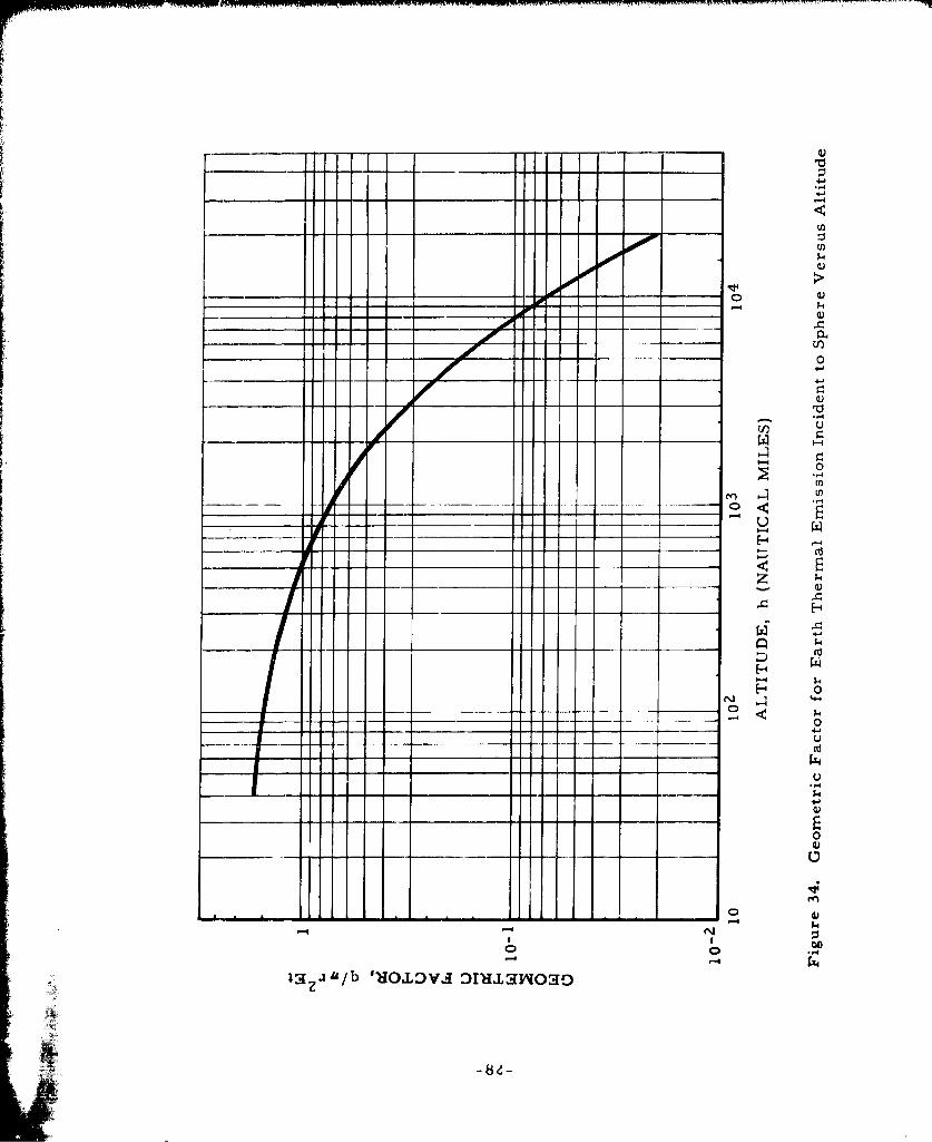
rn

0

1-

0A

00

4.5-

0

is aji/b '1O.LDV3 DIHLaWOao

CYLINDRICAL BODY--

Figure 35.~ Geometry of Planetary Thermal Emission to Cylinder

The radiant heat flux incident to the lateral surface of a cylinder ofdimeter D and length L from the element of planet surface ds is

DL sin AEt cos a dsdq- t (77)

where DL sin ,% is the projection of the cylinder surface as seen from ds,and Et cos a/n' is the energy radiated in the direction a. The values of H,cos a , ds, and p2 are given again by Equations 71 through 74.

The value of sin A is

-sin A = /1 - (cos 6 cosy + sin 6 sin Y cos 9•Z(78)

-83-

i.h

WN - wu w ~ w-nn~nr w.-- --.- rn---r-. -

where

Cos 5 H - R cos ) (79)p

sin - R sin 0 (80)P

After substitutions and some algebraic manipulation, the total incidentheat flux from the planet to the cylinder can be written as

ZD LEtR (H cos - R) sin 0 X (81)

f J (H +R 2 - 2RH cos 0)2

(V/A+B cos - C cosZOq dgd9)

where

A = Rz + H2 -H cos Y - 2RH cos 6 sin Y- R cos 0cos Y (82)

B = 2R 2 sin 0 cos 0 sin Y cos Y - 2RH sin & sin Y cos Y (83)

C = R sin20 sin2 Y (84)

Equation 81 cannot be integrated analytically; a numerical integrationis required. To perform this, and other numerical integrations mentionedlater, the solutions were programed on an automatic digital computer. Theresults are plotted in Figure 36, where the values of q/DLEt are given as afunction of the altitude above the earth surface h, with the attitude angle Y' asa parameter.

To apply the curves of Figure 36 to a vehicle in the proximity of aplanet other than earth, the same procedure and correction term as given forthe case of the sphere may be used.

Emission to Hemisphere

The configuration for a hemispherical body is shown in Figure 37. Theorientation parameter Y' for the hemisphere, although similar to that for acylinder, must assume values throughout 180 degrees because the hemisphereis only symmetrical about one orthogonal axis.

-84-

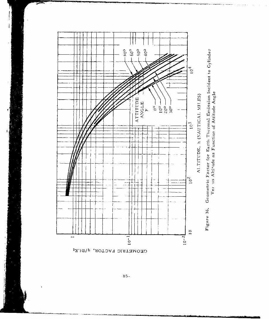
00 00

CD 0

14-

J.Lzo 0 0 0

f-4

toF

4aI,/ ____o~ - C)apoa

HEMISPHERICAL BODY

Ya%

P h

SPLANET R!

Figure 37. Geometry of Planetary Thermal Emission to Hemisphere

The radiant heat flux incident to the hemispherical surface of radius r

from the element of planet surface ds is1 z(12 n7r (cos A + 1) Et cos a ds

dq = (85)

where 1/2 urr (cos A + 1) is the projection of the hemispherical surface asseen from ds, and Et cos a /n is the energy radiated in the direction a. Thevalues of H, cos a, ds, and p2 are given again by Equations 71 through 74.

Tile value of cos A is

cos A cos 8 cos Y + sin 8 sin Y cos (86)

where cos 6 and sin & are as defined in Equations 79 and 80.

-86-

After substitutions and algebraic manipulation, the total incident heatflux from the planet to the hemispherical surface can be written as

ff90q = Ej rR (H cos R- R) sin 0 d6d9

qEo(r+ R -RH cos 3/2d)

(87).0o+ ! (H cos 0 -R) sin 0 (A + B cos! ) d~d95

f H R -2RH cos 0)600f

where

A = H cos Y - R cos 6 cos Y

B = R sin 6 sin Y

The first term of the integration may be performed analytically to givethe heat flux as

r 2ZR h+ h 2 '"t H / (88

+ R 0 (H cos R) sin 0 (A + B coso)d~d,

(Hz +R -2ZRH cos 0) 2

o00

The second term was integrated numerically. The results are plottedin Figure 38, where the geometric factor q/n'r2 Et is given as a function ofaltitude h above the earth's surface with the attitude angle Y as a parameter.These curves may be used for other planets as explained for the case of thesphere.

Emission to Flat Plate

For a flat plate, an integration method similar to that explained forspheres may be used. However, a similar solution can be found by resortingto a geometrical method of obtaining the view factor.

It can be proved that the view factor of a surface from a small flat platecan be geometrically determined. The surface is projected from the viewingpoint onto a sphere having its center at the viewing point. The image on the

-87-

_i I " '

ý4

o 0

0000'

0-4

_ -441

0

___ 0

-4-

I 0

000

43C ulb 'HO~Loya DIjjLL3NOa

sphere is then projected onto the plane of the small flat surface. The viewfactor is then determined from

F area projected on plane (89)- rV1

For this case, the surface is the region of the planet which the flatplate can see, and the radius of the sphere is taken as the distance betweenthe plate and the tangency point T, as shown in Figure 39. The generalcase, in which the plane of the plate intersects the planet, will be analyzedfirst.

The area of the circular segment A1 is

A yd (W d sin j1(A1 = 360 2 1 (90)

To obtain the value of (alp

oi = 180-2.A (91)

S= sin- 1 b (2#ksi (92)

b h+xb = h-+- (93)tan Y

h + x = p sin 0 (94)

sin 0 = H (95)H

2h + x = p (96)

H

2.

b p P (97)H tan Y

R ( 8d = pcosG80 = P1" (98)

R- tanY

-89-

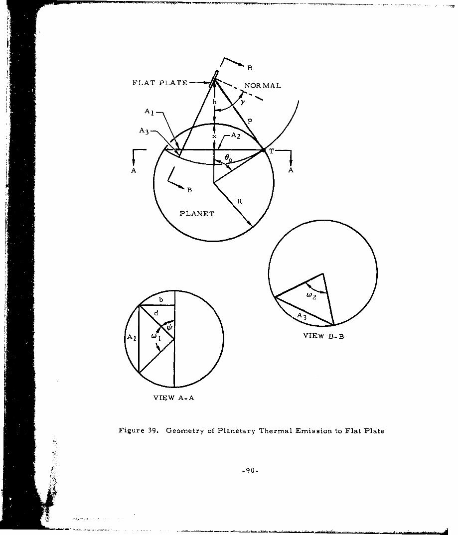
FLAT PLATE NRM

-- YA3 rp

VIEW B-B

PLNE

b ,.

Alm W I IW

i! ! !VIEW A-A

S.....Figure 39. Geometry of Planetary Thermal Emission to Flat Plate

-90-

and since

-I VH -R

(aI = 180 -Z sin Rtan (100)

The area A, is subtracted from rd to give A The area of the circularsegment A 3 is

2 2.rr p 'Z p sin c.2

A 3 360 = (101)

As for w., it can be found that

C2 - 180 - 2 sin J42 (102)

The view factor is obtained, then, by projecting the areas A2 and A 3 on theplane of the flat plate, and dividing the sum of their projections by 7rp 2 . Theresulting expression is

1I 1ýl/ H - R-']1 .l/H zRz1F - 1802 s Zin sin [2 sin-

'JR2 - H R410- sin' (103)

+H 2 3 6 0 H 180 - Z sJin- VR -'a R (103)

+ z-• Rtansin 2 sin-I a V /Jj cos Y

.t• much simpler expression is obtained when the plane of the plate doesnot intersect the planet. In that case A1 = A 3 = 0 and A2 = nd2 . Then

Az cos Y R2F2--cos Y (104)S2 12

In either case, the total heat flux from the planet to the flat plate isgiven by

q = Et F P (105)

•, -91 -

where P is the area of the plate. Figure 40 is a plot of the thermal radiationto a flat plate as a function of altitude with the attitude angle Y as a parameter.Again, to apply these curves to planets other than the earth, the proceduregiven for the sphere may be used.

* PLANETARY REFLECTED SOLAR RADIATION

As mentioned earlier, planetary albedo is the ratio of reflected to totalincident solar radiation. As such, the units of the term albedo are dimen-

. sionless; however, the expression has been used more and more frequently inrecent years to mean the reflected energy itself. Whatever the final, precise

i* ,definition of the term, it clearly differentiates the portion of the incidentsolar energy which is reflected by the planet from that which is absorbed andreradiated.

The average albedo for planets located up to 10 astronomical unitsfrom the sun is known with reasonable accuracy, the value for the earth beingthe least accurate. At distances greater than about 10 astronomical unitsfrom the sun, the accuracy of the planetary albedo falls off significantly

because of the very small magnitude of the reflected energy.

To permit a parametric analysis of the solar energy reflected from aplanet, the same assumption which was made for thermal radiation (i. e., auniform planet surface with regard to radiation characteristics) will be made.It is further assumed that the planet surface reflects diffusely (i.e., it obeysLambert's law). While these assumptions may not be entirely accurate,particularly for the earth where large bodies of water exist, they can bejustified by consideration of vehicle trajectories, orbits, and velocities usedin the analysis.

Based upon these assumptions, it is clear that the reflected energy hasa cosine distribution, not only with respect to the angular radiation from agiven area but over the sunlit surface of the planet as well. This consider-ably complicates the problem over the case of thermal radiation, with theresult that a direct analytical solution is not available even for the case of aspherical vehicle; for the cases of vehicles other than a sphere, the numberof computations is greatly increased by the increased number of variables.The result is that some 97 pages of curves are necessary to adequately

_ describe reflected heating to the sphere, hemisphere, cylinder, and flatplate which were used in the thermal radiation analyses. As a consequenceof the bulk involved, these albedo heating data are included as Appendix B of

this report.

.m As in the case of the thermal radiation analysis, the heating data isplotted in :eference to the earth. Also, the data may be used for vehicles in

the proximity of other planets by applying the same radius ratio correctionterms to obtain an equivalent earth altitude and then using the appropriate

ilimm mmm

o

0 o o o o r:)

't Ln D r-

-1'- 00 - o pole. w--U)

a-

C) 0

0

00

~av~b ~ j~ ~uw~oa

-93-

ordinate multiplying factor. This factor takes into account the albedo andsolar heat input to the planet considered.

Reflected Solae to Sphere

Considering the reflected (or albedo) heat flux incident to a spherein space, the most general configuration is given in Figure 41. As inthe case of thermal radiation, this heat flux to a sphere of radius r fromthe element of planet surface ds is

z

dq - nrr Ea ds (106)P

where

E cos a=rEa -

SPHERICALBODY

h SUNP

ds

I I Figure 41. Geometry of Planetary Reflected Solar Radiation to Sphere

I0-94-

Ii SHADE

S]lrimrR

•PLANET

Fiur 41.Il Geoetr ofPaeayRfetdSoa aito oShr

is the fraction of reflected solar radiation in the direction determined by a.Er is the total reflected energy per unit of planet surface, and is given by

Er = Sa cos fl (107)

where S (the direct solar heat flux normal to the sun direction), a, and / areas shown in Figure 41. Then

2

dq 2 Sa cos a cos f ds (108)

The values of cos a, ds and p2 are given by Equations 72 through 74. Thevalue of cos/3 is

cos i3 = cos 0 cos 0S + sin 0 sin OS cos (109)

By substituting these expressions inEquation 108 and integrating for 0and 0, q can be obtained. Careful consideration, however, has to be given tothe limits of integration. Two cases should be considered, as illustrated inFigure 42.

The first occurs when the region of the planet seen from the satelliteis completely sunlit. This condition can be expressed as

wherein the limits of integration for 0 are 0 and 00 and for ¶4 are 0 and at (theintegral with respect to ¶4 is multiplied by 2).

When the region of the planet seen from the satellite is only partiallysunlit,

00 > -0s

wherein a variable upper limit for ¶4 has to be introduced. It is convenient toperform the integration for two regions, as shown in Figure 42. Region 1 istotally sunlit, and the limits are 0 to 77/2 - OS for 0 and 0 to r for 95. Thelimits for region 2 are v/2 - OS to 0 o for 0 and 0 to a/2 + sin-' (ctg as ctg 0)for 0. 'rhis variable limit can be obtained as follows. From Figure 42 it is

evident that

IT+ 1: (110)

-95-

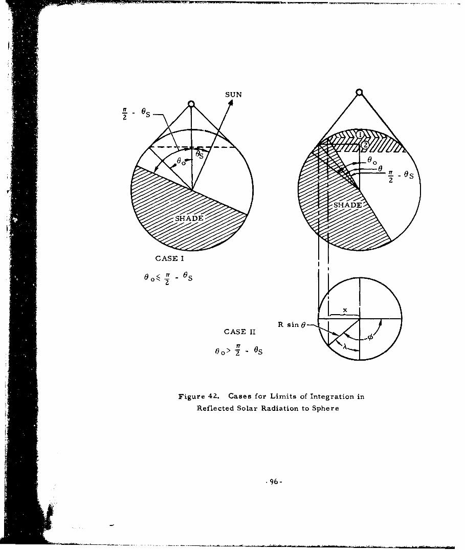
SUN

CAE

Oc- 0

SO

CCASE I

00> O-

Figure 42. Cases for Limits of Integration in

Reflected Solar Radiation to Sphere

.96-

Also Vx = R cos 0ctg% (I1i)

and

sin Rsin ctg 0 ctgO (112)

Therefore

-+ sin (ctg 0 ctg0) (113)

A S

Finally, by adding the integrals over regions 1 and 2 in Figure 42, the totalsolar radiation reflected by the planet incident upon the sphere is

A A T f- (Hcos 0 -R)(cos 0 cos (9S+ sin 1sin S cosk)sin0dOdoo o (R +H - ZRH cos 6) 3 /2

rr +(H sin-I(ctg 6S ctg O)

ArAS~f (H cos 0 - R)( cos 0 cos 0~ + sin 0 sin 0~ cos q,)sin OdOdq$aj S 0 (R- + HI " RH cos0)

2 (114)

Equation 114 holds for 0S< vT/1. For OS >- rr/i, the first term disappearsand the lower lower limit on 0 of the second term becomes O(S - if/A.

Integration with respect to r is immediate, but not so with respect to 0which requires a numerical method. Figure 43 shows the value of q/rrr 2-Sa,which is the heat flux to a sphere per unit of great circle (projected) area perunit of reflected solar radiation, as a function of altitude above the earthsurface, with OS as a parameter.

Reflected Solar to Cylinder

The albedo to a cylinder is computed by a numerical method similarto that used for a sphere; however, the integrand is more complex becausetwo additional parameters defining the attitude of the cylinder must beincluded. The general configuration is shown in Figure 44.

-97-

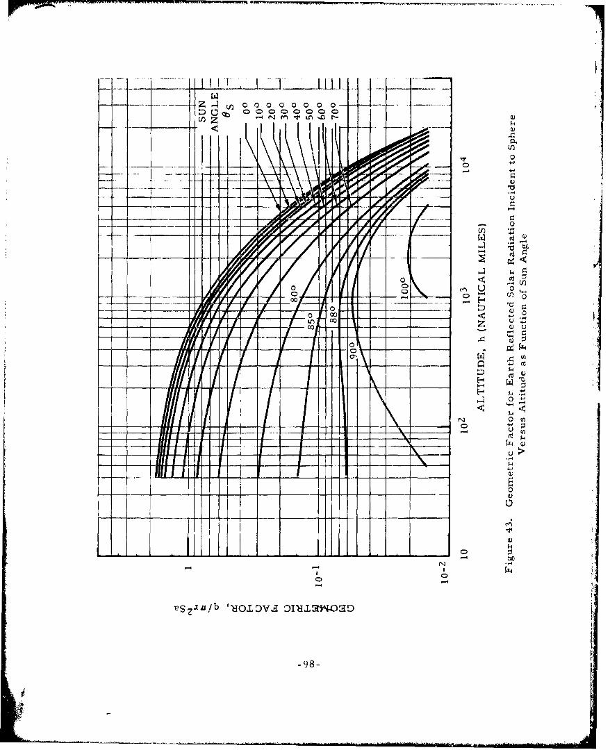
pol ~ ~ PL L LiI III. wi IMOMRI MRpNR i RM

- ~ ~ ~ ~ l M.- ----p zn -o r- 4) 0 0 0Lo Z

tc

4-4

1-4s

FI _

-9-4

CYLINDER

h

J TERMINATOR

Figure 44. Geometry of Planetary Reflected Solar Radiationto Cylinder

The radiant heat flux incident to the cylinder lateral surface of diameterD and length L due to reflected solar energy from the element of planetsurface ds is

DLE sinAds

dq = (I115)

I\-

where

E cosa

Ea = r

T M A

Figre44 Gomtr o Pantay efecedSo-99-iaio

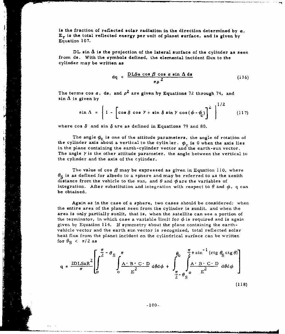
is the fraction of reflected solar radiation in the direction determined by a.Er is the total reflected energy per unit of planet surface, and is given byEquation 107.

DL sin A is the projection of the lateral surface of the cylinder as seenfrom ds. With the symbols defined, the elemental incident flux to thecylinder may be written as

dq DLSa cos P cos a sin A ds (116up

The terms cos a, do, and p2 are given by Equations 72 through 74, andsin A is given by

sin A = 1 - 6cos, cos Y+ sin 6 sin Y cos(4-0) (117)

where cos 8 and sin 6are as defined in Equations 79 and 80.

The angle 5c is one of the attitude parameters, the angle of rotation ofthe cylinder axis about a vertical to the cylinler. Oic is 0 when the axis liesin the plane containing the earth-cylinder vector and the earth-sun vector.The angle Y is the other attitude parameter, the angle between the vertical tothe cylinder and the axis of the cylinder.

The value of cos 8 may be expressed as given in Equation 110, whereOS is as defined for albedo to a sphere and may be referred to as the zenithdistance from the vehicle to the sun, and 0 and 95are the variables ofintegration. After substitution and integration with respect to 0 and 0, q canbe obtained.

Again as in the case of a aphere, two cases should be considered: whenthe entire area of the planet seen from the cylinder is sunlit, and when thearea is only partially sunlit, that is, when the satellite can see a portion of"the terminator, in which case a variable limit for 0 is required and is againgiven by Equation 114. If symmetry about the plane containing the earth-vehicle vector and the earth sun vector is recognized, total reflected solarheat flux from the planet incident on the cylindrical surface can be writtenfor 9S < -7/2 as

+ +sin- (cts ctg )]il,__O s "7 0 2s oZDLSaRZf A* BI C" D B - C D

Ir Vf 2 d~d5 + f A.B2G dOdo

-O 0- -= -'-1O(118)

-100-

where

A = Hcosn- R

B = coso0 cos 0+ sin s sin 0cos 9SS S

C - sin0

Z 2Z ZD YRZ +H' ZRHsin ycose-HI coo Y-R coo YcosO

- 2 RH co Yasin Ysin Ocos(O -

+R 2coo Ysin Ysin 0ocos cos(- )-R sin0 Vain2 Zcos (•- Z c

E = R2 + H -2 ZRH coso 0

Whenilmm i -Ss -Z+0+o

the integration limits change and integration occurs over only one zone withlimits given as

0 -o + sin (ctg 0, ctg 0)

ZDLSaRq f fABCD dOd9 (119)

E2

002 0

The heat flux integrals (Equations 118 and 119) have been integrated

numerically on an IBM 704 computer. The results are tabulated inAppendix B as the geometric factor (q/DLSa) as a function of altitude with2enith distance OS, angle between the vertical to the cylinder and thecylinder axis Y and angle of rotation OC of the axis of the cylinder about thevertical to the cylinder referenced to the plane containing the vertical andthe earth-sun vector (Figure 44). The values considered for the attitudeparameters were Y' = 0, 30, 60, and 90 degrees and simultaneously c =0, 30,, 60, 90, 120, 150, and 180 degrees. The parameter Y need only beconsidered to 90 degrees as the cylinder has end-for-end symmetry.

-101-

-HEMISPHERE

Pds ,

TERMINATOR

Figure 45. Geometry of Planetary Reflected Solar Radiationto Hemisphere

Reflected Solar to Hemisphere

The solution for albedo to a hemisphere is very similar to that for acylinder, the two major differences being that the expression for theprojected area of the hemisphere with respect to ds is somewhat differentand that values of y from 0 to 180 degrees must be considered because end-for-end symmetry is not present. The general configuration for albedo toa hemisphere is shown in Figure 45.

The radiant heat flux incident to the hemispherical surface of radiusr due to reflected solar energy from the planet surface ds is

-102 -

1 2

dq (I • 1+cOsA) Eads (120)2P

where 1/2 T•r 2 (1 + coo A) is the projected area of the hemispherical surfaceas seen from ds and the remaining symbols are as defined for a cylinder.Thus, the elemental incident heat flux to a hemisphere may be written as

1 2-,wr Sa costicosa(l+cos A) dsdq - 2 (121)

1TP

The term cor A is given by

cosoA = cosycosS +sinysin8cos(s - 0c) (122)

with the terms defined as for the cylinder solution. Again, cor o is givenby Equation 109, and cos a, ds, and p 2 are given by Equations 72 through 74.

The integration techniques and limits are as defined for albedo to acylinder. The total reflected solar heat flux from the planet incident onthe hemispherical surface can be written for OS< 1r/2 as

2 2[S fa AS-.B. G(VE+ F)ddq = r SaR j2

0 o (123)

- +sin- (ctg 0SctgO)

+ A-•A B'C (f-E +F) dOd If - 0S f2

whe re

A Hcoso0- R

B coo 0S cos O+ sinO0 sin0cos

C = sin0

E = R + H - 2RH cosr0

F = H cosry- R coo-ycos O+ R sinysin0cos(o- Oc)

-103-

When

illl< 0o <_ 1+SS! 0!

the heat flux to the hemisphere is

00 -~sin- (ctg 0 ctgO)

q = rSa ABR(V Ff o7E f d 0 d9d (124)

S2 E

The heat flux integrals (Equations 123 and 124) have been integratednumerically on an IBM 7090 computer. The results are displayed as thegeometric factor q/ v rz Sa as a function of altitude with the three angles0S, Y, and Oc as parameters. This tabular presentation is given inAppendix B. The values considered for the attitude parameters were 0, 30,60, 90, 120, 150, and 180 degrees for y and simultaneously 0, 30, 60, 90,120, 150, and 180 degrees for Oc.

Reflected Solar to Flat Plate

The most general configuration used in considering the albedo heatflux incident on one side of a flat plate in space is given in Figure 46.Development of the integral takes the same form as that for a cylinder or

a hemisphere. The heat flux incident to a flat plate of area P from theelement of planet surface ds is

•--- IP cosAEadsdq = (125)

where P cos A is the projected area of the plate as seen from ds. Since theremaining symbols to be defined are identical to those for a cylinder,Equation 125 may be written as

dq -P Sa cosf~cos acoosAds (126)"fp2

wherein cos y, ds, and p 2 are given by Equations 72 through 74, and cos 6

is given by Equation 109.

The term cos A is given by Equation 1 Z2, with the terms defined asfor the cylinder solution. The tdtal reflected solar heat flux from the planetincident on the flat plate can be written as an indefinite integral.

-104-

-FLAT PLATE

N•OR MAJL

p hS~SUN

0i /3,•mmR

•m •j •TERMINATOR

Figure 46. Geometry of Planetary Reflected Solar Radiationto Flat Plate

q PSaR AfB -C (G + F) do (12)

where A, B, C, and E are as defined for a cylinder, and

F = R sin y sin o cos( - 0 c

G= cosy (H-R cos09)

The problem of limits for the integration of Equation 127 is severelycomplicated in that the plane of the flat plate may cut off portions of thesunlit area of t.Le planet.

-105-

- -' - - - '

The limits considered are discussed with respect to the computersolution of Equation 127. Two major conditions are considered: (1) if the

flat plate sees the sunlit surface of the planet with the plane in which it lies

not cutting any portion of the sunlet area, and (2) if the plane of the flatplate cuts the sunlit area. If the plane does not cut the sunlit area, two

conditions may be involved. Either the plane sees a full sunlit zone (i. e.,

does not see the terminator), in which case Equation 127 becomes

0 172 Psa• R 2 A-'B" C (G + F"d) d,(ISq = 2 r f fEZ dOdi (128)

E0 0

or the plane sees part of the terminator, in which case, when 0 < ff2,

Equation 128 becomes

o o

q 2PSaR A. -B.C (G + F) dOdj9

~E2

0 0o

or ~+ sin- I(ctg O ctg 0)

when

then

ZPSaR A B" C (G + F)c (130

The problem becomes more complex when the plane cuts the sunlitarea because the limits of 0 and •/ are determined by" more complex

S~equations. If the plane cuts the sunlit area but the plane does not see thei!• terminator, Equation 127 becomes for 0S f12/ and V < /Z

+ iiff2 O

-106-

PSaR2[f A*BC (G+F) dodS

f fE2(131)

~ njtan [co- /R hR s..inO )]

tatan a!2

+PsaR f f A. B.C (G + F)

detrfnin] fr2 sHnaint co+s1

J=C tan Y)

where 0was determined by the Newton-1Raphson iteration procedure for

For /2< Y < iT/Z + 0o, q is given by Equation 131 with the firstintegral term eliminated. It should be noted that for y > f/2 + ro, q is

equal to O, (i. e. , the plane surface does not see the earth).

A number of forms of Equation 127 are possible if the plane of theflat plate cuts the sunlit area and also sees a portion of the terminator.

For the case where the plane of the flat plate for Y < r/2 intersects theterminator in two points, (03, 0 3) and (564, 04), and 03 and 04 > 00,S> 954, and 94 < ir, Equation 127 becomes

-107-

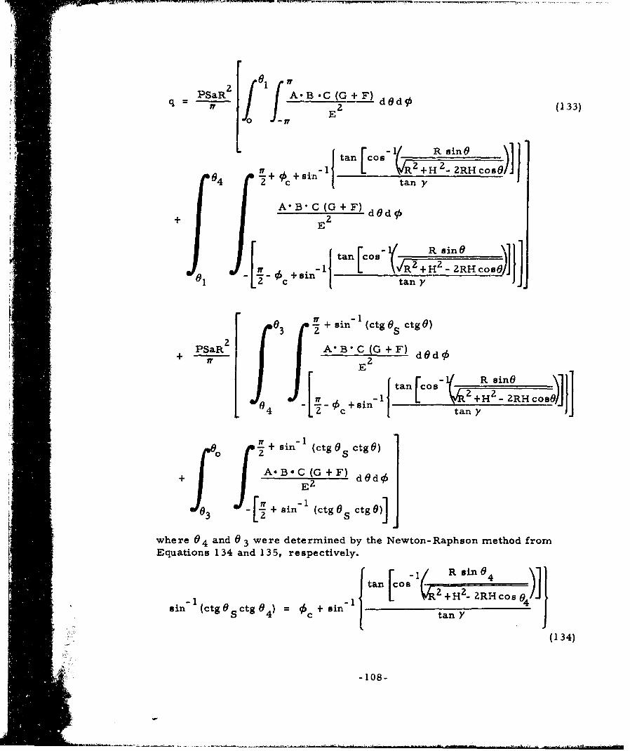
PSaR A.B.C (G + F) dOdIqo= �2E (1.33)

+s~~~~~In tan [co1, RnO )I[4si%+n i-- VR2 H ----RHcos 0)]

04 + .c tany

A-_B" C (G + F_) dOd

01 t I

R s a n 0

Z L -1-

03 + sin 1 (ctg 0 ctg O)

PSaR2 A* B' C (G + F)+ 1?2 dOd2

tan ICos R sin

64~~~ j2_2 sn ]Jsin-1 V 2 +H 2 _RH cosO4 - C i tan y

7 +-sin (ctg 0sctg 0)

A -B -C(G+ d0d+

0•3 4-asin (ctgOS ctg 0

where 04 and 0 3 were determined by the Newton-Raphson method fromEquations 134 and 135, respectively.

rm t a n 0 a- 1 i• k + -H Z R I -s i n 0 4J

sin (ctgOsctgo 4 ) = ¢+sin" t' I 1 1

{a 408-tanY

(134)

-108-

[ 1< co R sin 03co )ttanca

-ain-ltgScg3) I'¢ -si- I3

(CtgOS Cg 03 octan Y

(135)

For 04 > ",two conditions may be considered. If n/2 - 0 <1,Equation 127 becomes

PSaR A- B- C (G + F)q -2 d0do (136)

O - ir

0+ sz+Sin- (ctg0sctg0)

S B-C (G + F) d0d•fJ E2

" S" [z+sin' (ctggsctgO

-1 R sin0

)tancos -1 2+H Z RHcos)]

04 - + 9 +sin tan y

2PSaR A-B- C (G + F)+ fr E d0do

[ + sin 1(ctgs 0ctg 0]

03 + sin- 1 (ctg S ctg 0)

!1 3 E- -d-d-

Jos-l RsinG )]ff t ~ hl i an ~ c s0 d> c sin- 1 I t kVrR + Hz _ 2RH cot Q,

1, 12!tan y

-109-

S--

•r -1+sin- (ctg ctg 1

0sR. 2PsaP-g A• B_ .C (G + F)dd5

p -I- I

-+sin (ctg0s ctg0))

03 is determined by Equation 135, and 04 is determined by

tnR s in 0 4

tan |Cos •Z"

S+sn~ L VR+H - RH coos041v + sin- (ctg 0 ctg 04 =•ctn,

(137)

If r/. -0S > 01., the limits change somewhat.

01

of0tan [co- i sin 0

-2- OS + + sin- to 'tn

+A'B'C (G+F) dOd

+m 2

E2

0]~ ~~~~ RI~ csni ~o a sin 0

n 0tan[cos'('R R siLn0 -, A1f 1c V2+-2 + 2Hz cosH o s(/

. +sin-" )InlJ

2 * c __n

+PSaR f A -B C(G +F) dOdo +J 2fff_6 f-[ + sin- (ctg 0 ctg 0)J

-110-

2-+ sin-1 (ctgs ctgo)

A'B'C (G +F) dOdO/

tan cOs- R sin 0

-- 0 j S si='{ \+H. ZRHcos82 S 2 ctan >'

+ aR (ctg 0ctg0)

+ 2S AB C (G + F) dd

f0 f -[+ sin- (ctg0S ctg0) j

For the case where the plane of the flat plate intersects the

terminator in one point, (0 4 1 04), and the circle defined by 9 = 0 in one

point, (A3, 0o), and 54 < 7, Equation 127 becomesf0PSaR Af B C (G + F)

q d-0d (139)

tan os- 1R sinG

94 + +sin 1 tan -ZRHcos j+ A'B C (G + F) dOdS

2

+~ ~ sin1 14

tni Cos--- - - -

-i + sin-2 zRHcosi)- c tan Y

L

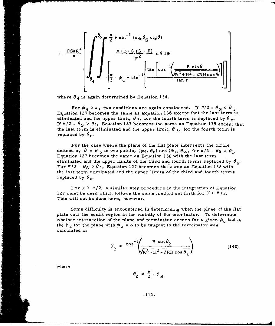
00 + sin- (ctg 0 ctg 0)

+PSaR 2 A-BC(G+F) dOd-

4 [un+o{tan Cos-

+R sin( )]

+• sin- p~R •Z .H2_2 o )

For 4 > iT, two conditions are again considered. If -7/2 - 0 S <Equation 127 becomes the same as Equation 136 except that the last term iseliminated and the upper limit, 0 3, for the fourth term is replaced by 0 0.If i1/2 - OS > 01, Equation 127 becomes the same as Equation 138 except thatthe last term is eliminated and the upper limit, 0 3, for the fourth term isreplaced by 00.

For the case where the plane of the flat plate intersects the circledefined by 0 = m in two points, (04, 00) arid (0 3, Go), for v/2 - OS KEquation 127 becomes the same as Equation 136 with the last termeliminated and the upper limits of the third and fourth terms replaced by o0.For I 7/2 - Os > 01, Equation 127 becomes the same as Equation 138 withthe last term eliminated and the upper limits of the third and fourth termsreplaced by Oo.

For Y > r1/2, a similar step procedure in the integration of Equation127 must be used which follows the same method set forth for Y <- 7r / 2.This will not be done here, however.

Some difficulty is encountered in determining when the plane of the flatplate cuts the sunlit region in the vicinity of the terminator. To determinewhether intersection of the plane and terminator occurs for a given 1c and h,the Y 2 for the plane with = o to be tangent to the terminator was"calculated as

Y2 Cos __________ (140)

whe re

0 r r-112-S

The maximum possible Y0 without intersection with the sunlit areawas then calculated as

y C9 (141)

Corresponding to this point is an angle, q6 co calculated from

=2sin- (ctg 0 ctg ) (142)

For a given 95c the limiting Ylim for intersection of the plane of the flatplate with the terminator was calculated from

Y'i - - (143)

This is not an exact determination of the Y for tangency of the plane of theplate with the terminator circle; however, the error introduced is small..

The heat flux integrals were integrated numerically on an IBM 7090computer. The results are presented in Appendix B as the geometricfactor (q/PSa) as a function of altitude with the three angles, 0 S, Y , and ,as parameters. Each table is for a constant Y and Oc

The albedo data for a flat plate is also useful in determining albedoto an irregular surface. The irregular surface may be approximated by aseries of flat plates and the albedo input is obtained by summing theindividual values for each of the flat plates.

-113-

DISCUSSION OF ASSUMPTIONS

SIMPLIFIED SPACE RADIATION ANALYSIS

1. It is assumed that all thermal radiation considered in the analysis isin diffuse form except direct solar radiation. Fortunately, most

* thermal radiation is in diffuse form, which is relatively simple toanalyze when compared with specular radiation.

2. It is assumed that direct solar radiation impinges upon the earth andupon the satellite with parallel rays, due to the great distance betweenthe sun and its planets. Almost zero error is introduced into theanalysis by this assumption.

3. In all cases, it is assumed that the earth emits as a black body and isin a state of thermal equilibrium (i. e. , the planetary emitted energyis equal to the absorbed solar energy). It is also assumed that theearth emission is a constant at any point on its surface and does notvary from day to night. These are reasonable assumptions becauselittle is known of the actual spectral and local variations in theplanetary emitted radiation.

*4. The earth reflected solar radiation is assumed to follow the cosinelaw Ii. e. , it is a maximumn at the sub solar point and decreases tozero at the terminator). This assumption greatly simplifies theanalysis and is quite accurate except in the region of the terminator,where a slight error is introduced.

5. In all cases, the planetary albedo is assumed to be constant over thesurface of the planet, and the planet is assumed to be a diffusereflector. This is done because of the complications of the problemand because local variations are almost impossible to define.

6. In all cases, conduction and convection between the satellite and itssurroundings were neglected. This is reasonable because orbital

heights are usually too far above the atmosphere for thermal effectsto appear.

7. It is assumed that the absorptivity to direct solar radiation of thevehicle surface is equal to the absorptivity to the earth reflectedsolar radiation. This is correct if the spectral quality of the

-115- IPREVIOUS PAGEIS BLANK

reflected solar energy is the same as for the direct solar energy. It isfelt that only a very small error is introduced by this assumption.

8. No transient heat transfer effects are considered in this analysis.Steady-state conditions are assumed for purposes of simplification.

9. An earth-oriented vertical cylinder is the assumed condiguration in allcases for purposes of simplification. The ends of the cylinder areignored in the analysis. The cylinder wall is assumed to be at auniform temperature, which is correct for a vertical cylinder spinningon its axis or for a cylinder with a shell of very high thermalconductivity.

10. In the discussion on simplified geometry analysis the earth is assumedto be a flat plate. This, in effect, results in the satellite-to-spaceconfiguration factor and the satellite - to- earth configuration factorboth being equal to 0. 5.

11. In the refined geometry analysis discussion, the earth is assumed to bea sphere. As a result, this analysis is considerably more accuratethan the simplified geometry analysis.

IBM 7090 PROGRAM FOR TRANSIENT HEAT TRANSFER ANALYSIS OFORBITING SPACE VEHICLES

.1. It iL assumed in this analysis that the earth can be representedgravitationally by the zero-order and second-order sphericalharmonics of its potential. The presence of harmonics in the earth'sgravitational potential causes periodic and secular variations inseveral of the orbital elements. Only the secular perturbations whichresult in regression of the nodes and advance of the perigee positionare considered in the analysis. Other periodic changes have negligibleeffect upon the shadow intersection problem.

2. A rigorous specification of the position at which the satellite entersand exits the earth's true shadow leads to needlessly complicatedexpressions. For this reason, the following simplifications concerningshadow geometry were assumed:

a. The earth was assumed spherical with its radius equal to 3960statute miles.

b. The earth's shadow was assumed cylindrical and umbral (sun atinfinity).

c. Penumbral effects were ignored.

-i16-

The error involved is extremely small even when large orbits areconsidered. For instance, a satellite in a circular orbit with analtitude of 10, 000 miles has an orbit period of approximately 560minutes, with perhaps 50 minutes spent in earth shadow (depending onorbit orientation). By assuming a cylindrical earth shadow andignoring penumbral effects, the analysis uses an umbral shadow timetHat is about 50 seconds longer than the true umbral shadow time. Thisis a negligible error. For a 1000-mile-altitude circular orbit, thenegligible error is approximately 18 seconds in an orbit period of 118minutes. Additionally, it should be mentioned that the assumption ofno penumbral effects tends to lessen these errors introduced by theassumption of cylindrical umbral shadow, so that there is almost zeroerror from a thermal analysis standpoint.

3. It is assumed that all thermal radiation considered in the analysis,except direct solar radiation, is in diffuse form. Fortunately, mostthermal radiation is in diffuse form, which is relatively simple toanalyze when compared with specular radiation.

4. It is assumed that direct solar radiation impinges upon the earth and-upon the satellite with parallel rays, due to the great distance betweenthe sun and its planets. Almost zero error is introduced into theanalysis by this assumption.

5. In all cases, it is assumed that the earth emits as a black body and isin a state of thermal equilibrium (i. e. , the planetary-emitted energyis equal to the absorbed solar energy). It is also assumed that theearth emission is a constant at any point on its surface and does notvary from day to night. These are reasonable assumptions becauselittle is known of the actual spectral and local variations in theplanetary emitted radiation.

6. The earth reflected solar radiation is assumed to follow the cosinelaw (i. e. , it is a maximum at the subsolar point and decreases to zeroat the terminator). This assumption greatly simplifies the analysisand is quite accurate except in the region of the terminator, where aslight error is introduced.

7. In all cases, the planetary albedo is assumed to be constant over thesurface of the planet, and the planet is assumed to be a diffusereflector. This is done because of the complications of the problemand because local variations are almost impossible to define.

8. In all cases, conduction and convection between the satellite and itssurroundings are neglected. This is reasonable because orbital heightsare usually too far above the atmosphere for thermal effects to appear.

-117-

9. It is assumed that the absorptivity of the vehicle surface to planetarythermal emission is equal to the emissivity of the vehicle surface.Since the effective temperature of the earth and the temperatures ofmost vehicle surfaces are nearly the same, this assumption isvalidated by Kirchhoff's law.

10. Any scattering effects of direct solar radiation upon the satellite due tothe earth's atmosphere are ignored. It is felt that this will introduce anegligible error into the analysis.

11. The geometrical configuration factor from the spherical satellite toearth was calculated with the assumption that the satellite is a pointsource in space. The assumption is valid if the satellite is uniformin temperature; it would be if spinning or if its shell had a veryhigh thermal conductivity.

12. It is assumed that any internally generated heat load is uniformlydistributed over the particular vehicle surface specified. Internalheat transfer paths are neglected. This was done in order to simplifythe analysis.

SPACE THERMAL ENVIRONMENT STUDY

1. It is assumed that all thermal radiation considered in the analysis,except direct solar radiation, is in diffuse form. Fortunately, mostthermal radiation is in diffuse form, which is relatively simple toanalyze when compared with specular radiation.

2. It is assumed that direct solar radiation impinges upon the earth andupon the satellite with parallel rays, due to the great distance betweenthe sun and its planets. Almost zero error is introduced into theanalysis by this assumption.

3. In all cases, it is assumed that the earth emits as a black body and isin a state of thermal equilibrium (i. e. , the planetary emitted energyis equal to the absorbed solar energy). It is also assumed that theearth emission is a constant at any point on its surface and does notvary from day to night. These are reasonable assumptions becauselittle is known of the actual spectral and local variations in theplanetary emitted radiation.

4. In all cases, the planetary albedo is assumed to be constant over thesurface of the planet, and the planet is assumed to be a diffusereflector. This is done because of the complications of the problemand because local variations are almost impossible to define.

-118-

5. In all cases, conduction and convection between the satellite and its

surroundings were neglected. This is reasonable because orbital

heights are usually too far above the atmosphere for thermal effects

to appear.

-119-

I,

Section VI

TECHNIQUES FOR RADIATION HEAT TRANSFER PROBLEM SOLUTION

GENERAL ANALOG HEAT TRANSFER ANALYSIS METHODS

NOMENCLATURE

A Area, sq ft

CE Electrical capacitance

CT Thermal conductance, Btu/(hr)(*F)

Cp Specific heat, Btu/(lb)(°F)

F Configuration factor

f Ihterchange factor

hc Convection heat transfer coefficient, Btu/(hr)(sq ft)(° F)

hr Radiation heat transfer coefficient, Btu/(hr)(sq ft)(° F)

I Current flow, amp

k Thermal conductivity, Btu/(hr)(sq ft)(" F/ft)

L length, ft

q Heat flow, Btu/hr

RE Electrical resistance, ohms

RT Thermal resistance, hr(° F)/Btu

t Temperature, * F

At Temperature difference at time 0

At Temperature difference at time 0

V Voltage potential

V° Voltage potential at time 0

0 Time, hr

a Stefan-Boltzmann constant : 0. 1713 x 10-8 Btu/(hr)(sq ft)(*R4

-Mass, lb

SRVOUS -PAG. ii li7 : "'"""'< 4

ELECTRIC CIRCUIT ANALOGY

The basic equations governing the flow of electricity are similar tothose governing heat flow; therefore, a close analogy exists between theconcepts of an electrical circuit and a "thermal circuit. In complicatedheat transfer problems it is often necessary to rely upon this analogy toarrive at the solution.

In the thermal circuit, temperature difference is considered analogous

to voltage potential and heat flow is considered analogous to current flow.Thus, the analogous equations

I A (amp) (144)R RE

Atq (Btu/hr) (145)RT

Thermal resistance RT is evaluated with respect to the mode of heattransfer

RT L for conduction (146)T kA

R = h-A for convection (147)c

R 1T hA• for radiation (148)

r

where

hr = af(T1 2+ T 2 )(T 1 + T 2 )

It is often convenient to use the concept of thermal conductance insteadof thermal resistance. Conductance is merely the reciprocal of resistance.Thus

CT k for conduction (149)CT =-L'

C_ = h A for convection (150)± C

C = h A for radiation (151)

"STEADY-STATE AND TRANSIENT PROBLEM SOLUTION

An example of a simple steady-state heat transfer problem utilizingthe network method of solution is an insulated round wire carrying anelectrical current. The heat generated inside the wire is i R watts,which must be dissipated by conduction through the insulation and by

convection and radiation to the environment. The temperature of the wiretw and the ambient temperature ta are known. The problem• is to determinethe amount of heat dissipated and the temperature of the surface of theinsulation ts (Figure 47). It is convenient to combine RC and RR into asingle resistance as shown in Figure 48.

INSULATION CONVECTION

RC

CONDUC TIONtw 4ANv ts ta

Rl

RADIATION

RR

Figure 47. Thermal Network for Insulated Wire

CONVVEC TION&

CONDUCTION RADIATIONtw - - - A O ta

RI ts R 2

1

RC RR

Figure 48. Simplified Thermal Network for Insulated Wire

-123-

The total heat loss is given byt -t

q R Rw a (152)

and the surface temperature of the insulation is given byc tw+ C t

1 w 2 at , t = (153)

It will be noted that the discussion has been limited to steady-stateconditions. However, it is often required to analyze heat transfer problemson a transient basis (i.e., temperature versus time). In this case, theeffect of heat capacity must be included. The analogous equations fortransient conditions are

V = V e-O/RECE (154)": • ' 0

r•~~~ 0/RT (Oc)C(55

At = At e T p (155)]i • 0

where

At = Temperature difference at time 0 = ta - to

At = Temperature difference at time 0 = ta - to

It is evident that the term oc is the thermal capacitance. The thermalp"circuit for a single node, single resistor transient problem (represented in

Equation 155) is shown in Figure 49.

RT

t A ta

WCp

Figure 49. Thermal Network for Single Node, Single ResistorTransient Problem

Multiple node transient heat transfer problems are handled byconnecting a thermal capacitance between each node (temperature) andground. This type of circuit is difficult to solve by hand, and usually

F! requires the use of an analog or digital computer. The network for thetemperature distribution versus time in a sa.) might appear as shown inFigure 50.

I I I I I ita 0 0 0 0 0

ti tz t3 t4 t5 ttl i ,,• •3 I ,A Jl t5 , t6 I

ta

Figure 50. Thermal Network for Temperature DistributionVersus Time in Slab

p RADIATION HEAT TRANSFER ANALYSIS METHODS

NOMENCLATURE

A Area, sq ft

E Black body emissivity power, Btu/(hr)(sq ft)

F Configuration factor

i Interchange factor

G Sum of all incident radiation, Btu/(hr)(sq ft)

hr Radiation heat transfer coefficient, Btu/(hr)(sq ft)(° F)

J Radiosity of surface, Btu/(hr)(sq ft)

q Heat flow, Bta/hr

r Reflectivity

c iEmissivity

RADIOSITY A.,ALOG METHOD

Problems concerning radiation heat transfer involve proper accounting

of all inter reflections between the various objects, shields, and surfaces

being investigated. This can be achieved very satisfactorily by utilizing

the radiosity analog network method as developed by A. K. Oppenheim of

the University of California (Reference 16). The significance of this

technique becomes apparent when interreflections with multiple surfaces

are considered. Other methods of analysis, at best, can only approximate

interreflections for most cases. The radiosity method presents an analyti-

cally exact solution, without need for such items as "modified" configuration

factors.

The radiosity method is normally restricted to problems concerning

gray bodies; however, problems concerning real bodies can be analyzed if

the additional effort is warranted. It should be noted, however, that the

analysis is limited to diffuse emission and reflection, but radiation from

most surfaces is fortunately in diffuse form.

-4I27 - F V.AGNKS, ! IS SLAM

In describing this technique, it is important to define the radiosity ofa surface J. Radiosity is the sum of all the emitted, reflected, andtransmitted radiant energy streaming away from a surface. For a grayopaque surface, radiosity is the aum of the emitted and reflected radiationand is given by

J= rG + tE (156)

where

E= vT

Therefore

G= J- E (157)r

Al so

qbet = A(J - G) (158)

Substituting

qLqnet J - cE

= _ = J +- EA r r r

rJ-J

r r

(r"1)Jr r

S(E -J)r

Therefore

et = (E - J) (159)

Thus, the net radiation leaving or entering a surface is analogous to thecurrent flow when a potential of E - J is applied across a conductance oftA/(l -(1

-18

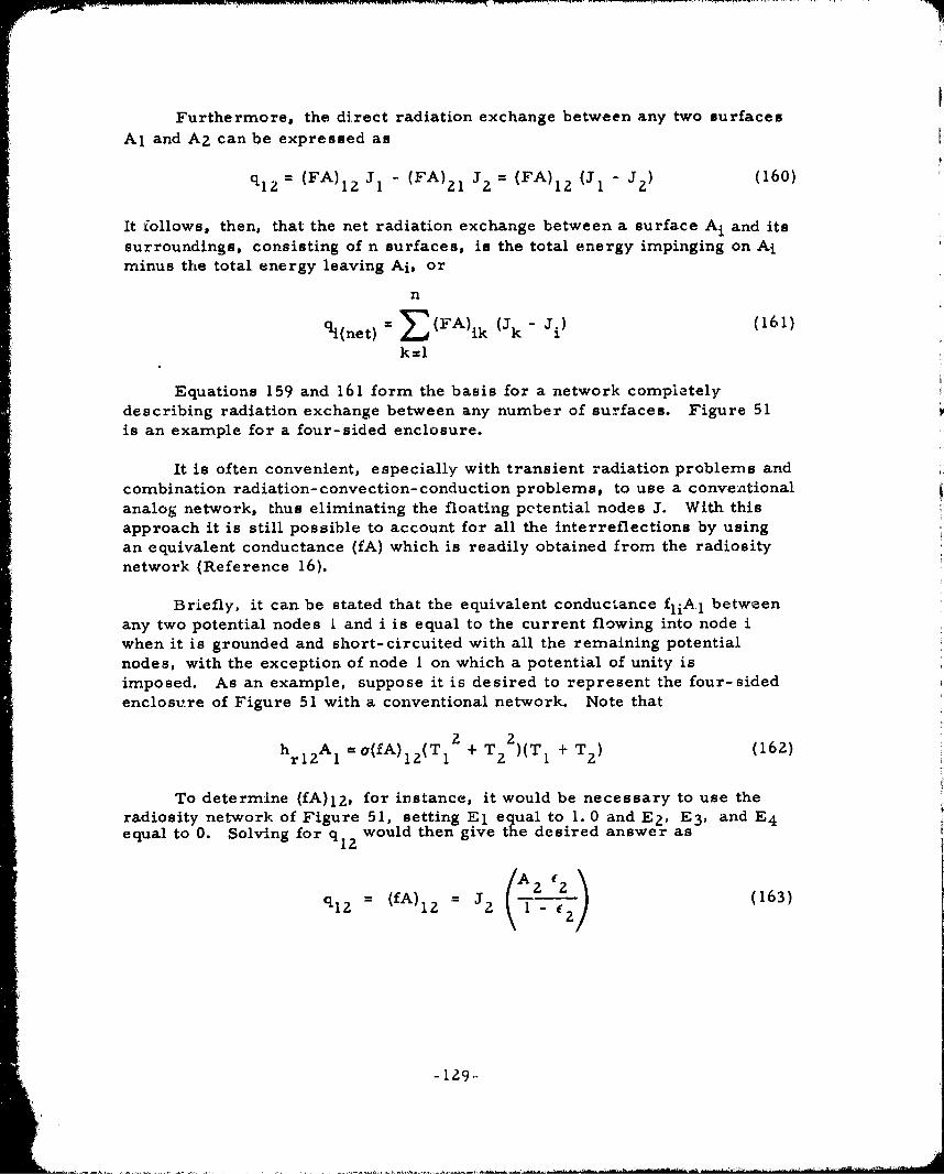
:• , . ..T•- ,• • • • • ,: ...... •: • ... . •i•,?w w• • ... ... r n n w - r - -... N-

Furthermore, the direct radiation exchange between any two surfacesAi and AZ can be expressed as

q12 = (FA)1 2 J 1 - (FA) 2 1 J 2 = (FA) 1 2 (J 1 - J12 ) (160)

It follows, then, that the net radiation exchange between a surface Ai and itssurroundings, consisting of n surfaces, is the total energy impinging on Aiminus the total energy leaving Ai, or

n

q1(net) = (FA)ik ( k- i (161)

k=l

Equations 159 and 161 form the basis for a network completelydescribing radiation exchange between any number of surfaces. Figure 51is an example for a four-sided enclosure.

It is often convenient, especially with transient radiation problems andcombination radiation- convection-conduction problems, to use a conventionalanalog network, thus eliminating the floating potential nodes J. With thisapproach it is still possible to account for all the interreflections by usingan equivalent conductance (fA) which is readily obtained from the radiositynetwork (Reference 16).

Briefly, it can be stated that the equivalent conductance fliA1 betweenany two potential nodes I and i is equal to the current flowing into node iwhen it is grounded and short-circuited with all the remaining potentialnodes, with the exception of node I on which a potential of unity isimposed. As an example, suppose it is desired to represent the four-sidedenclosure of Figure 51 with a conventional network. Note that

hr1 2 A 1 =-a(fA) 12 (T 12 + T 2

2 )(T 1 + T 2 ) (162)

To determine (fA) 1 2 , for instance, it would be necessary to use theradiosity network of Figure 51, setting El eqjual to 1. 0 and E 2 , E 3 , and E 4equal to 0. Solving for q1 2 would then give the desired answer as

q12= (fA)2 = J2 (163)-1292

-129-

T W M M P P R I m l ,I , M I M I I o n 1 m M 0 .W q tll "

E3 =a T 3 4

I Ie I

J

LeA

E4 ~~ ~ E =a TlT4 ý= Z

Figure 51. Radiosity Analog Network for Four-Sided Enclosure

-130-

/hr

In a like manner, the equivalent conductances (fA) 1 3 , (fA) 14, (fA) 2 4,(fA)2 3 , and (fA) 3 4 can be obtained and then used in the network of Figure5Z for the general solution to the problem.

COMMONLY USED METHODS

One of the earliest relationships for the net heat transfer between twobodies is the simplified equation from Hottel (Reference 17).

ql 2 = OeFaA (T14 T 4 (164)

where

F = Configuration factora

F = Factor which includes emissivities allowing for departure ofsource and receiver from complete blackness and which dependsupon c1' c. and configuration of surfaces.

A second method developed by Hottel (Reference 18) to evaluate the netexchange between two surfaces is expressed by

q1 f12 A 1(T 1 T 2j (165)

where

f "

F ~A12 1 2 2

and

F Configuration factor from surface 1 to surface 212

Equations 164 and 165 are limited in application with respect to multipleinterreflecting surfaces. An attempt has been made to account for reflecting(refractory) surfaces by replacing the geometric configuration factor F witha modified configuration factor F, which includes both direct and reflectedradiation effects. Values of'F are usually obtained from charts or graphsand are rather limited in application bt.cause these graphs are available forcertain specific configurations only.

,/ -131-

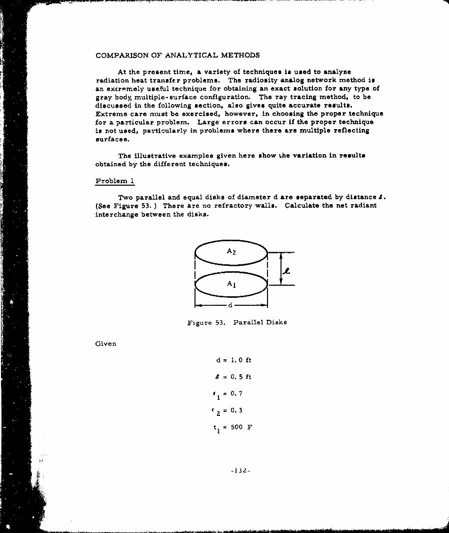
COMPARISON OF ANALYTICAL METHODS

At the present time, a variety of techniques ia used to analyzeradiation heat transfer problems. The radiosity analog network method isan extr'-mely useful technique for obtaining an exact solution for any type ofgray body, multiple- surface configuration. The ray tracing method, to bediscussed in the following section, also gives quite accurate results.Extreme care must be exercised, however, in choosing the proper techniquefor a particular problem. Large errors can occur if the proper techniqueis not used, particularly in problems where there are multiple reflecting

surfaces.

The illustrative examples given here show the variation in resultsobtained by the different techniques.

Problem 1

Two parallel and equal disks of diameter d are separated by distance e.(See Figure 53. ) There are no refractory walls. Calculate the net radiantinterchange between the disks.

d-

Figure 53. Parallel Disks

Given

d = 1. 0 ft

I = 0. 5 ft

1 = 0.7

Sz = 0.3

t= 500 F

-132-

=100 F

F = F 1 = 0. 37 (p 57, Reference 17)

Solution 1A

From Reference 17 (Equation 164),

q 1 2 e a 1 (T 1 4- T 2

where

F = f r = 0. 21 (p 56, case 10, Reference 17)

F =0.37a 2 2

A1 =I rr = 1r(0.5) = 0. 786 sq ft

T 500 + 460 = 960 °R

T = 100 +460 = 560 °R2

a= 0.1713 x I08 Btu/(hr)(sq ft)(0R 4 )

Therefore

q 1 2 = 0. 1713 (0. Zl)(0. 37)(0. 786)(9. 64 - 5.64)

= 0. 1713 (0. 21)(0. 37)(0. 786)(8500 - 983)

= 0. 1713 (0. 21)(0. 37)(0. 786)(7517) = 78. 6 Btu/hr

Solution 1B

From Reference 18 (Equation 165),

4 4q 12 af 1 2 A1 (TlI - T

where

f= 1

S12 =1 A2

-133-

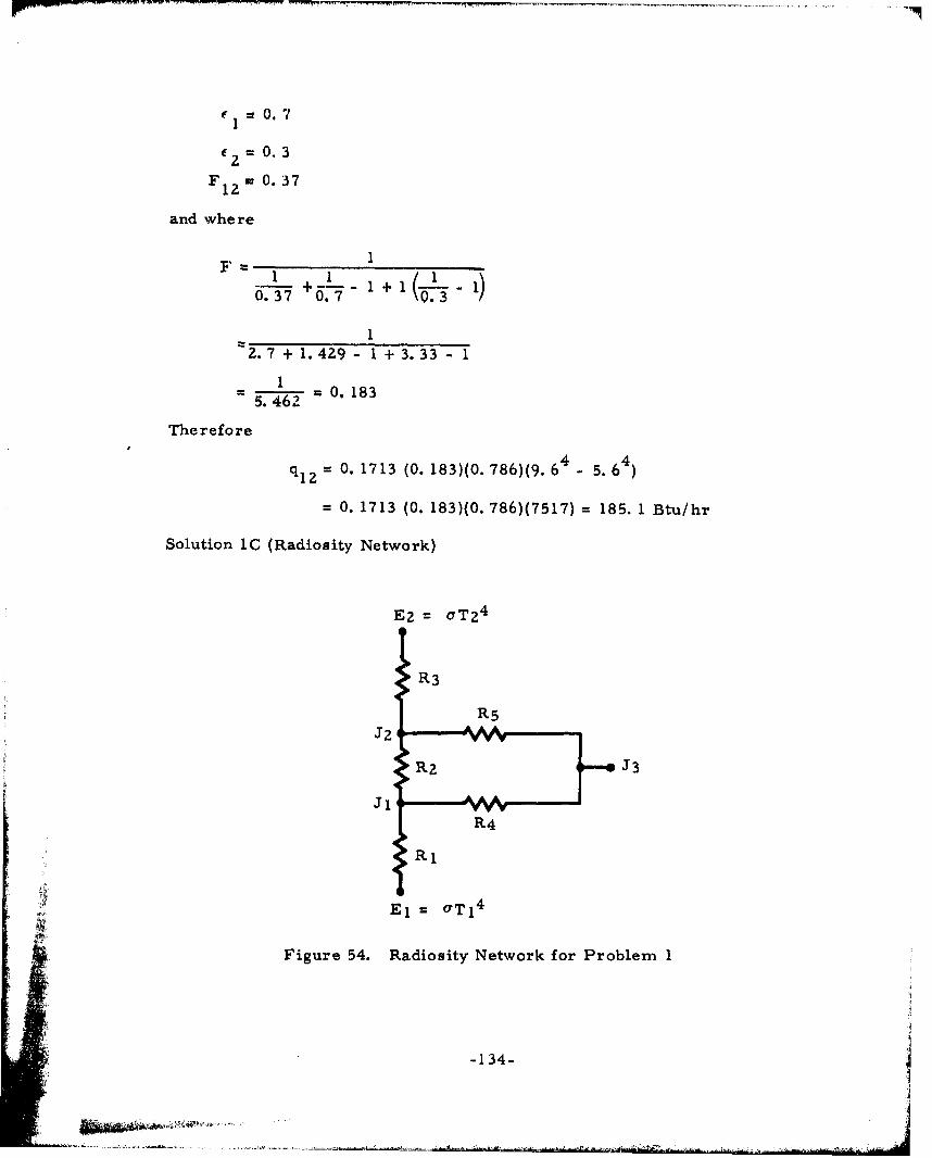
E0 =071

2 -0. 3E

F 1 0.3712

and where

0.7+F. 1 1 1

12. 7 +1. 429 - 1 + 3. 33- 1

1

5.462.=0.183

Therefore

q1 2 = 0. 1713 (0. 183)(0. 786)(9. 6 4- 5. 6 )

= 0. 1713 (0. 183)(0. 786)(7517) = 185. 1 Btu/hr

Solution IC (Radiosity Network)

EZ = aT24

R3

R5

J2L

S••.El= aT4

Figure 54. Radiosity Network for Problem 1

-134-

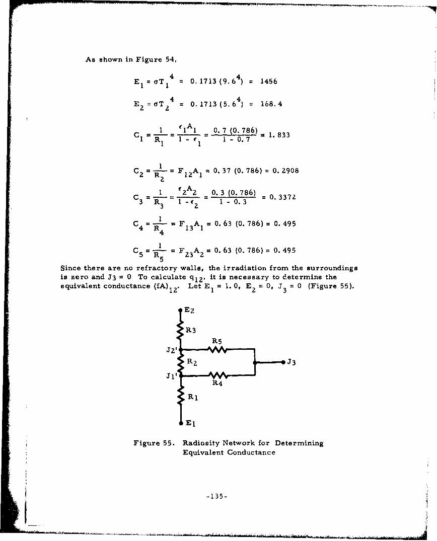
As shown in Figure 54,

4 4)E = 1T4 = 0.1713 (9.6 ) = 1456

4 4E E =T4T = 0.1713(5.64) = 168.4

C 1 '1A1 0.7 (0.786) = 1.8331 R T - 1 1 - 0.7

•Cz =Z F zA1 0. 37 (0. 786) 0. 2908

C 1i •2A2 =0.3 (0.786) =0. 3372

C3 R R3 =I- 1 - 0. 31 11

2 R. F 12 A I = 7.3(0. 786) =0.49584

C -=R-- F A = 0.63 (0. 786) = 0. 495

5R5 23 2

Since there are no refractory walls, the irradiation from the surroundingsis zero and J 3 = 0 To calculate q 1 2 , it is necessary to determine theequivalent conductance (fA)1 2. Let E 1 = 1. 0, E= 0, 13 = 0 (Figure 55).

E27

3R3

J211

R2 J3

pR4

Figure 55. Radiosity Network for Determining

Equivalent Conductance

t ~135-

I !

Solving forJI and jz

C (El - 'J) + C4 (J 3 l + C2 (3, " J = 0

C (E -J+ (+ )C -31 )03 2 2 5 21 2

1.833 (1 - J + C0,495 (0 - + 0.2908 (J, - J1) = 0

0. 3372 (0-2J+0. 495 (0• +o0. 2908 ( o1 =0

1. 833 + 0. 2908 J? - 2.6188 Ji = 0

0. 2908 3 'l - 1. 1?30 J = 0

J = 3.86 J.1&

J> - 0. 1868

Therefore

(fA) 12 C 3 (12 - 0) = 0. 3372 (0. 1868) = 0. 063

and

q1 2 = o(fA)12 (TI4 - T- 4

= 0. 1713 (0. 063) (9. 6 4- 5. 6 4 81. 2 Btu/hr

Discussion of Problem 1

If Problem 1 were recalculated for the case where F was 0. 9 insteadof 0. 37, the following comparison could be made:

Method FIZ = 0. 37 F12 = 0.9

Equation 164 78.6 Btu/hr 191 Btu/hrEquation 165 185. 1 Btu/hr Z62 Btu/hrRadiosity network 81. 2 Btu/hr 231 Btu/hr

As Oppenheim has pointed out in his paper (Reference 16), theradiosity network gives the exact solution to radiant interchange problems,with the basic stipulation that the radiant energy be in diffuse form. Thus itcan be stated that the answers obtained by use of the radiosity network forboth cases of problem 1 are the correct results. These are presented in thetable above as 81. 2 and 231 Btu/hour, respectively. Equation 164 is correctfor the first case but is about 20 percent in error in the second case.

Equation 165 is over 100 percent in error in the first case and about 15percent in error in the second.

-136-

Problem 2

Given

To show the effect of reflecting surfaces, let the configuration ofProblem 2 be enclosed with a single reflecting (refractory) surface. It isassumed that the reflecting wall reflects all the incident radiation.

Sol4tion 2A

From Reference 17 (Equation 164),

qjZ = FeFaA 1A(TI 1 T 24 )

where

F 2 =0.21 (p 56, case 10, Reference 17)

F = F = 0.64 (Figure 4-7, p 57, Reference 17)

Therefore

q 12 = 0.1713 (0.21) (0.64) (0.786) (9.6 - 5.64

= 0. 1713 (0. 21) (0.64) (0.786) (7517) = 136 Btu/hr

Solution 2B

From Reference 18 (Equation 165),

q q12 C flAI2TA " (T4q2 = 14

where

1 I

' -- + -- A1+-I--iS1F 1 2 +

=A

-1 = 0.7

f2 = 0.3

1z = 0.64

-137-

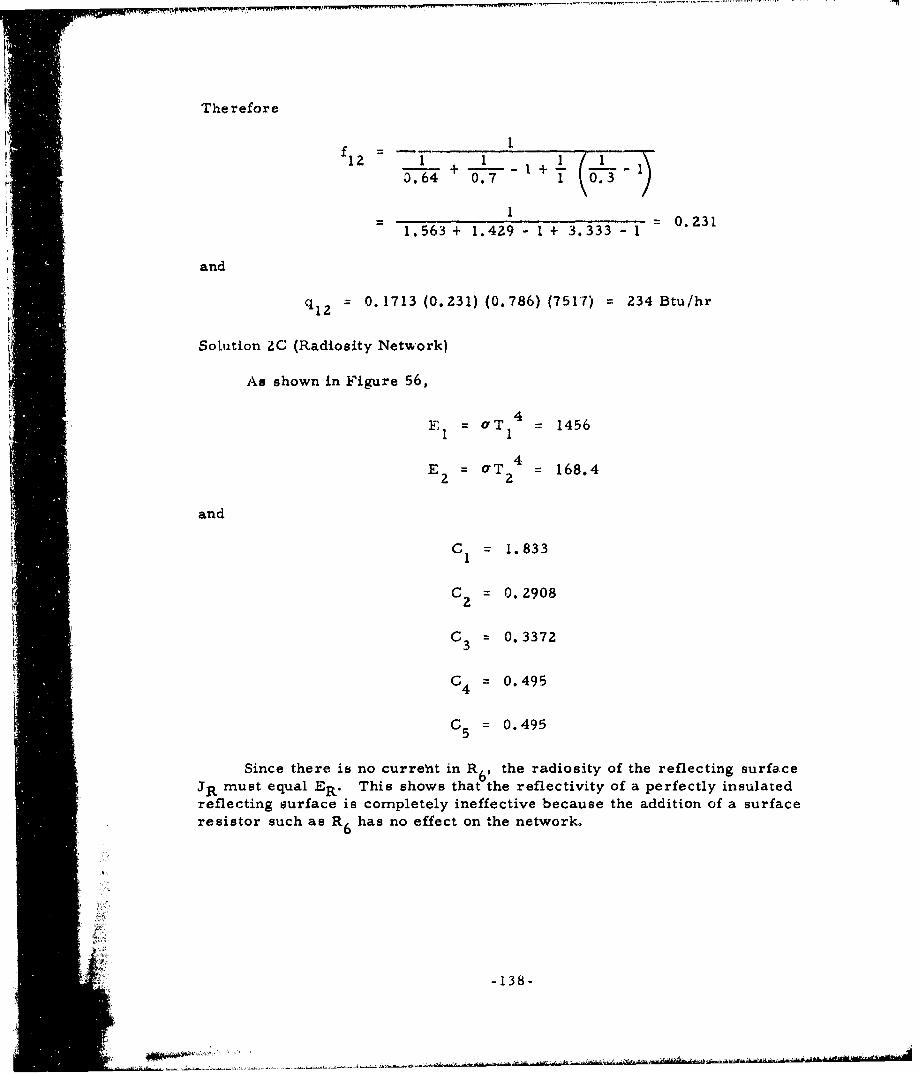
Therefore

t fl = 1

12 1 1 1 +

0.7. 231

1.563 + 1.429 - 1 + 3.333 - 1

and

-q = 0. 1713 (0.231) (0.786) (7517) = 234 Btu/hr

Solution 2C (Radiosity Network)

As shown in Figure 56,

4El = "T = 1456

if• 4E? = T = 168.4

2 2

and

C, = 1. 833i~m 1

Cz = 0.2908

C 3 = 0.3372

C = 0.4954

C5 = 0.495

Since there is no curreh1t in R 6 , the radiosity of the reflecting surface

JR must equal ER. This shows that the reflectivity of a perfectly insulatedreflecting surface is completely ineffective because the addition of a surfaceresistor such as R6 has no effect on the network.

-138-

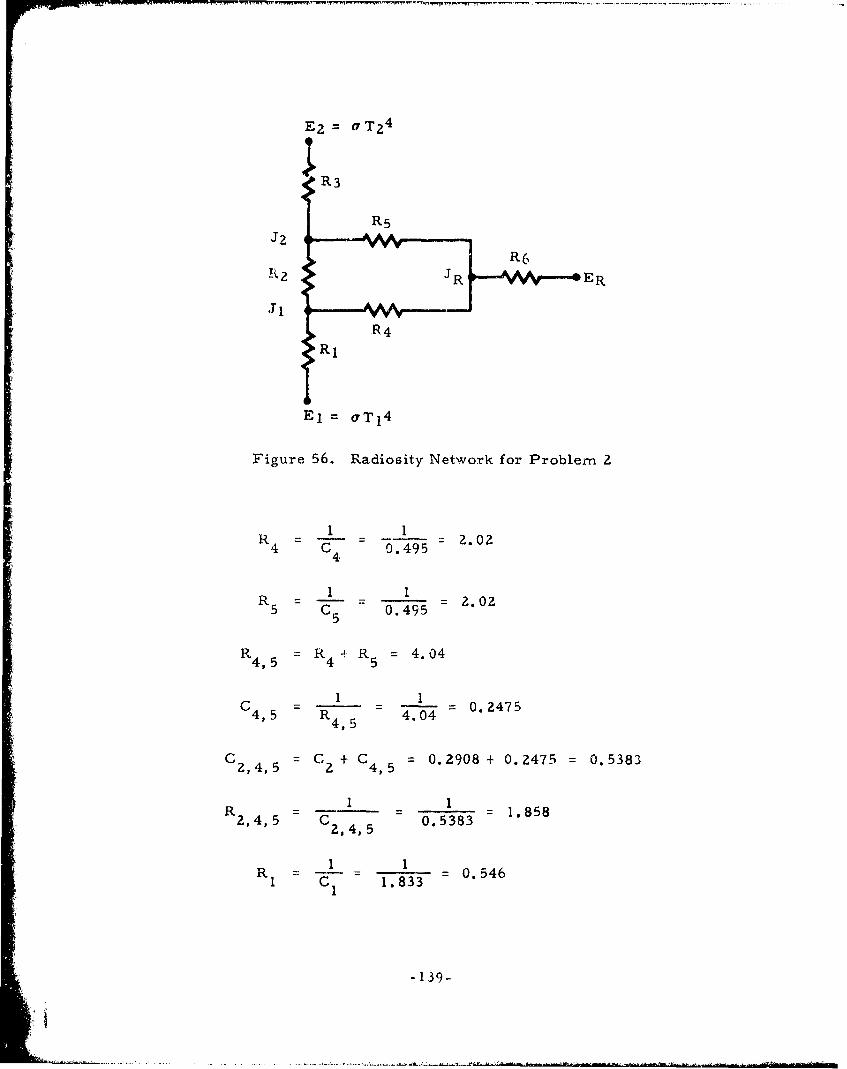
E "2 = T24

J2 R5

J I

T4S~R1

E1 = aT14

Figure 56. Radiosity Network for Problem 2

R. = -_ 1 2.024 C 4 0.495

1 1

R5 = I - • = 2.025 C5 09

R 4,5 = R 4 R5 = 4.04

1 1

C 1 - 1 0.24754,5 R 4,5 4.04

C2,4,5 = C2 + C 4,=5 0.2908 + 0.2475 = 0.5383

R - 1 - 1 = 1.8582,4,5 C 2 ,4, 5 0.5383

R = -.. 8 3. 5461 1 1.8331131

-139-

- -•. .

1 1R3- 3- 2.973 C3 0.3372

R R + R +R = 0.546 + 1.858 + 2.97 =5. 374total 1 2,4,5 3

Therefore

I

q = R (E1 - E2)total

1

5.374 (1456 - 168.4)

12Z87.618. 240 Btu/hr

5.374

Discussion of Problem 2

Problem 2 is summarized as follows:

Equation 164 136 Btu/hr

Equation 165 234 Btu/hr

Radiosity network 240 Btu/hr

In the case where interreflecting surfaces are present, it can be seenthat Equation 164 is in considerable error even with the use of a modifiedFa. In this case, however, Equation 165 is close to the correct answer of240 Btu/hour.

In reviewing the results of Problems 1 and 2, it is concluded thatEquations 164 and 165 are correct only if they are chcosen with care to buitthe problem at hand. The radiosity network method of analysis, however,is always correct for cases involving diffuse radiation.

-140-

RAY TRACING ANALYSIS METHOD

Very accurate results may be obtained from the ray tracing method of

heat transfer analysis. Unfortunately, however, the method is difficult touse without a high-speed digital computer because of the lengthy and tediouscalculations involved. A method has been developed whereby this technique

can be programed for an IBM 704 or 709 computer (Reference 19), although

the programing has not yet been none. The material for this discussion was

supplied by the Los Angeles division of North Amei ican Aviation.

NOMENCLATURE

a Area of surface

e Monochromatic emissivity power of black surface at particularsurface temperature and wavelength

f Configuration form factor

q Heat flow

u Energy emitted by surface

v Energy received by surface

W Energy absorbed by surface

Emissivity

X Wave length

p Reflectance

"RADIANT INTERCHANGE ANALYSIS

* ~This discussion is concerned with an enclosure made up o'f a finitenumber of finite surfaces. The enclosure contains a nonabsorbing media.

Each of the surfaces of this enclosure is considered to be opaque,homogeneous, diffusely reflecting, uniformly irradiated, and at a uniformtemperature. The it surface of this n surface enclosure emits :i.adiant

energy in the amount

U4 =a (1-P .)e1 .(AX). 0j 1,Z2... P) (166)

-141-

whe re

th

a, = Area of it surface

Pi, j = Reflectance of ith surface for radiation of average wavelengthA. in narrow wavelength band of

JJe = Mot.6chromatic emissive power of black surface at temperature

of i surface and at wavelength X

The term reflectance describes the behavior of a particular specimen,while reflectivity is reserved to describe the behavior of the material itself

(i.e., the reflectance of a highly polished specimen of a material is numer-

ically equal to the reflectivity of that material).

The right-hand side of Equation 166 actually represents p terms where

p is the number of wavelength bands into which the important part of theelectromagnetic spectrum has been divided. This notation convention will beused throughout this discussion. That is, whenever a subscript appears two

or more times in any product on the right-hand side of an equation and doesnot appear on the left-hand side of that equation, it is to be understood that

the product in question is to be summed on the subscript, as the subscripttakes on all of its possible identities.

The ith surface receives from the n surfaces directly emitted radiationwhich has suffered no reflections in passing from the originating surface to

the ith surface. This energy is in the amount

v =U f (k= 1, 2...n) (167)

o i, j k,ji ki

whe re

th jtif = Configuration factor from k to i surfaceki

In Equation 167, the subscript o denotes the fact that no reflections havetaken place in the transfer of the energy.

Of the energy ovi, j, the ith surface absorbs

0oWJu, j = k1-P i, j)Uk,j fki (168)

where, in the general case,

p0w i -:F 0 (169)

j= 1

-142-

-I . . - ---.-----.-.--- ,-._ -- - - 11-1-- --- 1 -

Energy which has suffered 0 reflections before reaching the ith surfaceis

Rv, -=..~ fPfP (170)juk.jfk I,jIm rnj mn n, j' "0si

The amount of this energy absorbed by the ith surface is

S(Uk, jfk.1PI, jfjmPm, jfmnPnj. . fs 1)(1-Pj) (171)

An energy balance on the ith surface for radiation of average wave-length X. isa

00

q 1 . =j = , 8-0. w., (172)

That is,

q, j , = (U- (I )(u3 1, j i, j k,jfki k, jfkePtjfei

Suk,j

fk X Ij j m i + ... ) (173)

where the energy qi, which must be added to or removed from the ith surfaceto take into account the differences between the radiant energy leaving andentering the surface, is

00

q,= q, j (174)j=0

The form of Equation 173 is not suitea to computations. Therefore,the procedures are directed tcward obtaining forms of the energy balanceequation that are more suitable for computation. The terms can be writtenas a product of certain matrices. For example,

f.

UVJf i [uiu .u ] [f U F (1) (175)

L-ni-

-143-

and

Iipj k, j k 1 g j i± ~ if11 f12'f In Pij, 0 ... 0 fLi

f f f 0 0 4I,

*21 " ' I2 0 0]. zi= U i, u ,* u n,

f f .*f 0 O., Pnl nnZ nn J L n,j Jni

= Uj Fj (i) (176)

The capital letters are reserved for matrix quantities unless otherwisestated. That is

U =j [ul,juZ, "''un,j] (177)

"f I I f " f In

f21 f2 "'f 2nF • • (178)

o 0L. f = .f . f f nn

0 0 Pn

n ~ n, nn

fli

f

F() . (180)

fnUni

Equation 173 can be written in the form

q, j =ui, j - (I Pi, [U F(i) + UjFRjF(i) + UjFRjFRjF(i) +

(181)

-144-

0 r

Si. j G1-pi, j )Uj [I + (FR ) + (FRi)' + (FRj) + ... J FMi) (18Z)

where

[10.. 0]

(183)

It can be shown that[+( j)(F ) (FRF.))2 .. ,]'1 [I-FR.]'I

+(FR) + (FR 3 (184)

where

_, -FR. is the inverse of the matrix I, - FR ]

Finally, Equation 173 may be written in the form

=qi, j ui, j - (, - Pj)Uj [I - FRjI F(i) (185)

The total net energy leaving or entering surface i is

= ui -(1 - P U.)U. [i - FR ]"1 F(i) (186)

The matrix equation for the entire system of n equations is

U - - R )U [1- FR.]- F (187)

where

Q = [qlq 2 ."'.] (188)

and

Un] (189)

-145-/I

DIGITAL COMPUTATION

For the purpose of digital computations of heat transfer and tempera-

tures of n surfaces, equations in the forrm of Equation 186 will be used. Let

Ci, jCl 2 'j. C In, jC C ...- 21, jCCl, J C2nj1(190)

C Co

nlj C nZj' ' Cnn, 'J

The matrix product in Equation 186 cin be shown to be

U F 'IR F(i)= u (c f +C f .4c fU - j l,jllj ii 12, j Zi +n, j ni

+U c f +c f ;l+. . +c .f2, 1,j fli 22,j 2n, j ni(191)

+Unjf, .( fli +c jf 21 . +c f )Unoj nl,j n2n,, Zi'" nn,/jni)

Planck's equation gives the relationship for monochromatic emissivepower of an ideal radiator at temperature T..

1

e C

=ijc (19 2)

8 exp T -l

where C is 1. 18070 x 108 Btu (microns) 4/(hour)(square foot) and C2 is25896 microns (*R), where microns is the measure of wavelength.

Let

- C Btu/fhr)(sq ft) (193)

exp -1

Then

-146-

- - - - - --(£,- -

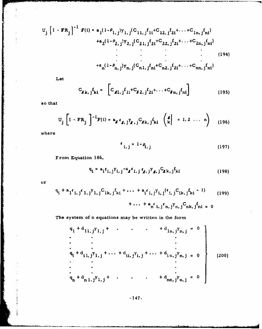
U~ [I FR 1 F(i) a a1 (1-P 1 J)Yll (c1 l .f11+C21 2 ~f i+.+ in f)

+s IP) C f+ +C f2 Zit 2 j 211 21 2, j21 n, j ni

*(194)

+a (1-P )y (C f+C C fn n,ji n, j nl ni, nj2 njn

Let

CJk, jfki = LCJIjfl~i+C 2, £jif 2i *n, 3fni] (195)

s0 that

J, [IFj 'Fi=aE jC~k J'k = 12 n (196)

where

Ei~ -p j (197)

From Equation 186,

qi = ai(,jj -aREj j j E jYACjk jfki (198)

or

qi +a1 f ,j ,j lk,j ck.jki i + i, jyi, j(i, jik, jfki 1 19

+ .. an ci, Jc n, Jy n, j cnk j fni =0

The system of n equations may be written in the form

q,+d i*yt + d l yn j 0

qa + d,1 y.,+. + d, jy *+j.+ + d1i1jl~ i~j ~jin,j n~j =0 (ZOO)

+n + d n ,Sl + d nn .v = 0

-147-

where

dap=a$ E J(D CPk, Jfka a) (201)

where a is the Kronecker delta andap

a1 = i0f a=.

The quantity qi may be heat that is conducted or convected to the surfacei or it may be that generated internally in the material of surface i. There-fore, in general, the system of equations to be solved for the unknown tem-peratures TV, T 2 ... Ti'...Tno Ta# Tbto'is

d11, jyl, J+. .+dln, jyn, j+do I IT 1+ +do InTn+doIIaTa+do lbTb+' + 371 = 0

dil, jYl, j+ '` +d n, jYn, j+dlilT+1 +di i nTn+dtIiaTa+dIibTb+''+ = 0

dnl, jyl, j+ +dnn, jYn, j +don1TI + . +d nnTn +dnaTa+dnbTb+" +17n = 0

Other equations containing only T to the first power equal zero.s

(202)

where Ta, Tb, and so forth, are temperatures of elements of the systemwhich are not involved in the radiant energy interchange. All terms havingthe primed coefficients are reserved, of course, for conduction and convec-tion. This assumes that the conduction and convection of energy can bewritten in such a manner that only the first powers of the temperatures areinvolved. The 17 terms are reserved for internal energy generation withinelements of the system.

It should be noted that this analysis has been set up using the assump-tion that Lambert's cosine law adequately defines the space density of emittedand reflected radiation. Obviously, this is not the physical case. A moreexact analysis would include the variation of space density of reflected andemitted radiation. However, because no such data are now available andbecause such a numerical analysis would be complex for even the mostadvanced computing machines, it has not appeared necessary that these moreaccurate descriptions of the actual physical system be included at this time.

-148-

The preceding analysis is general for the case ol varying values of

reflectance with wavelength. Here, again, -it would be a major task to

actually sum across the spectrumn and at the same time solve the required

set of nonlinear equations. Therefore, as a first step in probing such solu-

tions, it has been decided that a gray ',ody analysis should be used. This

simply moans that the quantity y will be replaced by aT 4 , This assumption,

of course, has been used many times in the past even though it often leads to

inaccurate solutions. It is not, then, necessary to sum on j in the expression

for d. in Equation ZO1.

i

- 149 -

-- I

DISCUSSION OF ASSUMPTIONS

I. The methods of analys1s discussed in this section have the commonrestriction that radiant energy is emitted or reflected in diffuse form,

as opposed to specular form. A satisfactory method of handling partlydiffuse, partly specular radiation has not yet been devised. Fortunately,most thermal radiation encountered in engineering applications can be

considered to be in diffuse form.

2. The radiosity network method is usually applied only to gray bodyradiation and is so used in this report. Mettods have been developed

whereby non-gray .-adiation can be treated, but this Is considered beyondthe scope of this report.

-- 151

r3Qou, AG

Section VII

CONFIGURATION FACTOR STUDIES AND DATA

CONFIGURATION FACTOR EVALUATION

. One of the most difficult areas in the analysis of radiation heat transferis proper calculation of the geometric configuration factor. Basically, theconfigura#ion factor F12 from A, to A 2 is defined as the fraction of the totalradiant flux leaving Al that is inciaent upon A2 . The configuration factorfroin a plane point source to a finite surface (commonly known at a differen-tial-finite configuration factor) is obtained by integration over AZ, and themean configuration factor from a finite source (finite-fir. te configurationfactor) is the average of the point configuration factors over the finite source.The integral expression for the differential-finite configuration factor fromd,AI to A2 is given by

fcosO9 cosO dAF(dA - A 2 12 (203)

A2

The integral expression for the finite-finite configuration factor fromA1 to A2 is given in the Section III discussion on radiant heat exchangebetween surfaces.

F12 =.L 1 12T ~ l (204)

A1 A 2

As an example (from Reference 20) consider the two mutually perpendi-cular surfaces shown in Figure 57. The )eft-hand corner of the horizontalsurface is assumed to be the origin, with the x, y, and z axes as shown. Thehorizontal surface has overall dimensions of D and W while those of thevertical are H and W. Thus

F 2 f / coso 1 coso0 2 dA dA 2 (205)

-153-

i N h m 1ih -m i

F- W-

x2 dAZ

A2

//S

z Al

D

IX S~dA1

x

it•gure 57. Geometry for Calculation of Configuration Factor for

• i' Two Mutually Perpendicu~lar Surfaces

where coo 1

S

S = ,X- xiZ + (D y)2 + z2

anddA dx 1 dy

dA = dxI dz

-154-

*.. .. . ... . •

I!iitherefore

H D WW-F' -f 7z (D - y)

2 F ýDr 2 -)dxldxzdydz

0,0 0d0 1(X2 X)2 +(D Y)+ +Z (206)

Integrating Equation 206 yields

1 �-• (D2 - W- + H2 ) In (D-+H 2 +WZ2

S(D2 +H-) in (DZ+H 2 ) - (D 2 - w 2) In (D 2 + WZ) (207)

WDI [ (HZ " W2) In (H2+W2) - DIn iD 2 - H' in H'+ W- in W2)

S1 -1W -1 W W+ WDr[HW tan- H + DW tan D- - W /v2 +H Wtan "I

V'D2 + HJ

It can be seen that the integration process is often tedious, even for simpleshapes such as in the example. In fact, for most cases the integrationcannot be solved analytically and. other means must be used to obtain theanswer. Under these circumstances the following approach can be utilized:

1. if the areas in question can be assumed infinite in one direction,there are several very simple and rapid rmethods available withwhich to obtain the configuration factor.

2. If step 1 does not fit the problem, the next step is to use tablesand charts which are available for specific configurations. Theseare discussed in this section and provide solutions to a numberof different configurations, with the help of form factor algebra.

3. If the previous steps are not adequate, there is available an IBMprogram which calculates the configuration factor between anytwo plane areas if they are in the form of parallelograms.

-155-

4. The method that can be used where all other methods prove tobe inadequate is called the unit sphere method. This is ahighly accurate techniques although unfortunately it is rathertedious. Most mechanical integrators are based on thu unitsphere principle.

A most useful method for evaluating the coidiguration factor betweensurfaces infinite in one direction is called the "string" method and is pre-sented in Reference 21 (p 66-68).

E

in2F

B

Al

Figure 58. Diagramn of Infinite Enclosure

Consider the enclosure of Figure 58. It is desired to compute the con-figuration factor from surface Al to surface A2 . A minimum-length line isstretched over the surface connecting edge B of K, to edge Z of AZ (dottedline BCDE) as well as a minimum-length line from edge L of A1 to edge F ofA2 (line LKJHGF). A minimum-length line is now stretched from B to F(line BHGF) a second line from L to E (line LKJE). The configuration factorF 1 2 can then be obtained from the expression

= A2F 2 1 (LKJE + BHGF) - (BCDE + LKJHGF) (208)

-156-

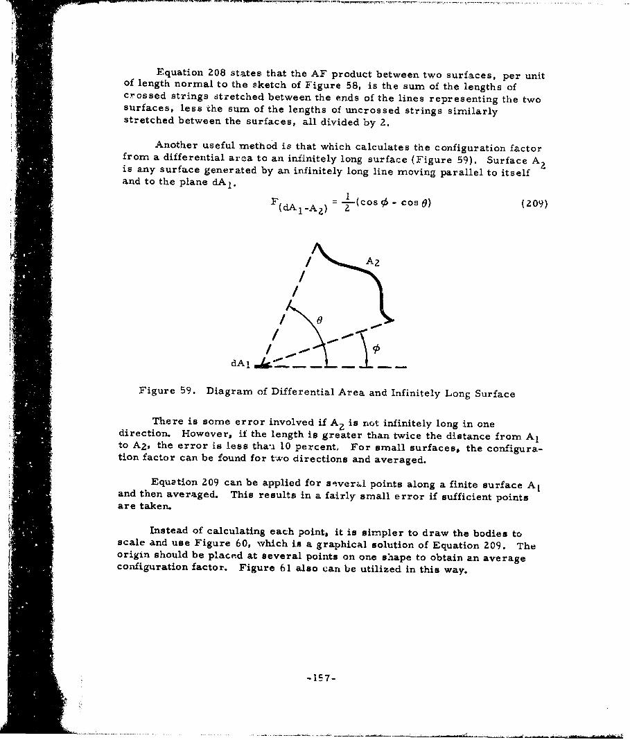
Equation 208 states that the AF product between two surfaces, per unitof length normal to the sketch of Figure 58, is the sum of the lengths ofcrossed strings stretched between the ends of the lines representing the twosurfaces, less the sum of the lengths of uncrossed strings similarlystretched between the surfaces, all divided by 2.

Another useful method is that which calculates the configuration factorfrom a differential area to an infinitely long surface (Figure 59). Surface A 2is any surface generated by an infinitely long line moving parallel to itselfand to the plane dA 1 .

(dA 1 -A 2 ) -2 -(cos cos 9) (Z09)

/ AA2

S/ 8

dAl

Figure 59. Diagram of Differential Area and Infinitely Long Surface

There is some error involved if A2 is not infinitely long in onedirection. However, if the length is greater than twice the distance from A1to A2, the error is less thai 10 percent, For small surfaces, the configura-tion factor can be found for two directions and averaged.

Equation 209 can be applied for setverzl points along a finite surface A1and then averaged. This results in a fairly small error if sufficient pointsare taken.

Instead of calculating each point, it is simpler to draw the bodies toscale and use Figure 60, which in a graphical solution of Equation 209. Theorigin should be placed at several points on one shape to obtain an averageconfiguration factor. Figure 61 also can be utilized in this way.

-157-

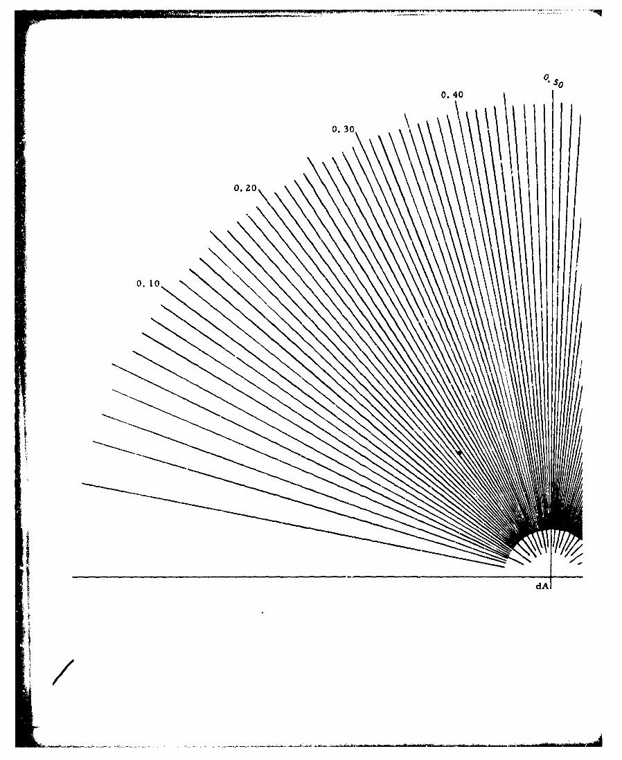
50

0.40

0. 30

0.20

0. 10

dI

0. 40 0.60 07

0.80

0

dAl

Figure 60. Differential Area Shape Factor for T

-159, 160o 1

- .- -- , '...r. W ~r . - r

0. 60

/ 0. 70

1/! / 0.80

0. 90

1.0

Figure 60. Differential Area Shape Factor for Two-Dimensional Case

-159, 160 -3

1. 00- 900700

•0.90 600

~500Z 0.80

45o

S~~300 -•

zw 0.50

C44

C• 0.400.4 LUNE

0

w0. 30 0 0

ANL 01(DGRES

€dA.

S• ~0.210 \

SFdA, L 1 /2 (sin 01 + sin Oz)

0o 10 20 30 40 50 60 70 80 . 90

ANGLE 0 1 (DEGREES)

Figure 61. Shape Modulus From Differential Area to Lune

-161-

I,TABULATED DATA

DATA OF REPORT NACA TN 2836

One of the most widely used sources of tabulated configuration factordata is report NACA TN 2836, "Radiant - Interchange Configuration Factors,"D.C. iramilton and W.R. Morgan of Purdue University, December 1952(Reference 22). This report includes configuration factor data for the follow-ing shapes:

1. A plane point source dA1 and a plane rectangle A2 parallel to the

plano of dA1

Z. A plane point source dA1 and a plane rectangle A?, the planes ofdAl and AZ intersecting at an angle 5(0-< 0 < 1800)

I•I• 3. A plane point source dAI and any surface AZ generated by an infi-

"nitely long line movin& 'arallel to itself and to the plane of dA 1

4. A plane point source dAl and any infinite plane A2 with the planesof dA1 and A 2 intersecting at an angle 69

5. A ipherical point source dA1 and a plane rectangle AZ

r 6. A plane point source dA 1 and a plane circular disk A2

7. A plane: point source dAI and a plane disk A 2 , the planes of dA 1 andA2 intersecting at an angle of 90 degrees

8. A plane point source dA 1 and a right circular cylinder A2

9. Two concentric cylinders with a point source dAI on the inside of

th3 large cylinder at ono end

10. Same geometry as shape 2 with a triangular area added to the top ofA2

11. Same a. shape 10 with the triangle reversed

12. An infinitely long cylinder Al and an infinite plane A2 , mutuallyparallel

- 163 -i BAiii

'"S I !tI11 qLH!

13. A line source dA1 and a plane rectangle A2 parallel to the planeof dA1 with dA1 opposite one edge of A2

14. A line source dA1 and a plane rectangle A 2 which intersects theplane of dA 1 at an angle

15. A line source dAl and a right circular cylinder A2 parallel todA1

16. Two concentric cylinders with a line source dA1 on the inside ofthe large cylinder. The outside cylinder is Al, the insidecylinder is A 2

17. Same geometry as shape 16, calculates configuration factor fromdA 1 to the ends of the concentric cylinders

18. Identical, parallel, directly opposed rectangles

19. Two rectangles A1 and A2 with one common edge and an includedangle ( between the two planes

20. Parallel, directly opposed, plane, circular disks

In addition to the graphical and tabular data presented in this report,the integrated equations of many of the shapes are given. Form factor algebraand basic theory are also presented.

DATA OF CONVAIR (FORT WORTH) STUDY

This discussion presents the results of a study conducted by the FortWorth Division of Convair to determine the configuration factors for variousshapes (Reference 23). No attempt has been made to present the derivationof the equations presented herein. A complete development of the equationscan be found in Reference 23.

It should be noted that some of the integrations cannot be performedanalytically and numerical methods are required.

Parallel Planes

For nodes 1 and 2, as defined in Figure 62, lying on parallel planes,the black body interchange factor is defined by the following equations.

- 164 -

Figure 62. Nodes on Parallel Planes

F2 = fl(-bb8-c) - fl(O-a,8-c) + f,(a-a, 8-c)- fl(a-b,8-c)

+ f 1 (a-b,Y-c) fl(a-a, Y-c) + f (1-a, Y-c)

- f I(,8-b, Y-c) + f (8 -b, Y-d) - -a. Y-d) +f (a -a, y-d)

- fI(a-b,y-d)+ f 1 (a-b,8-d) - fI(a-a,8-d)+ f (6-a, 8-d)

- f 6(8.b, 8_-d)) (210)

where the function f is defined by!I

SEvtan- 1 V Vz + -i t, (211)fllu,) = E~tn -g-• + tan Z + VZ

E 2. -E 2 E + v+-vE+ tan- m~m~ +- In )

2 2

- 165 -

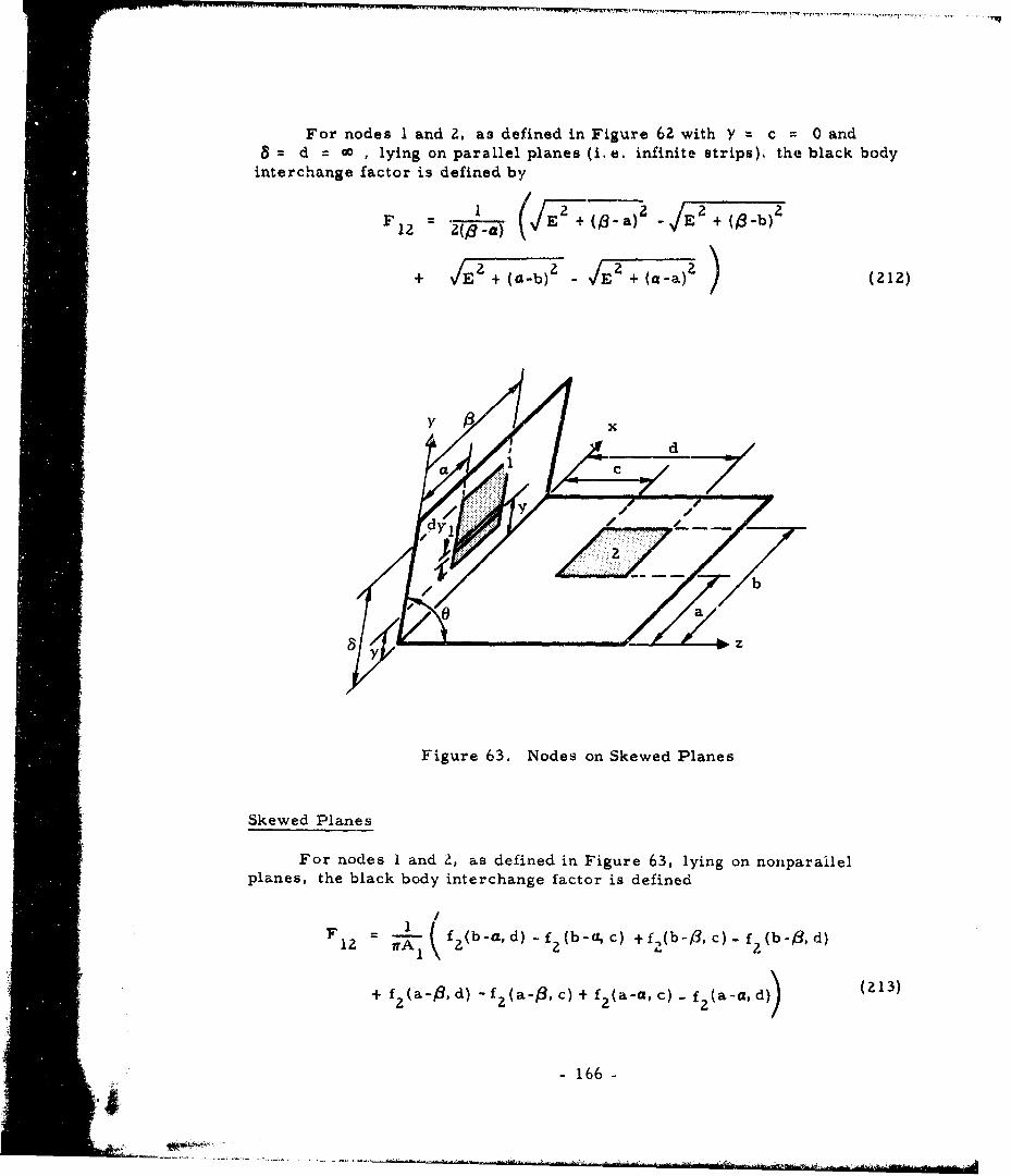
I low

For nodes 1 and Z, as defined in Figure 62 with y = c 0 andB = = d 0 , lying on parallel planes (i, e. infinite strips), the black body

interchange factor is defined by

F12 (a) ( ( a)2 -E + (-b)

12 +

+ /E2 + (a-b)" - fEi + (a-a)Z (212)

• " Figure 63. Nodes on Skewed Planes

; Skewed Planes

S~For nodes 1 and 2, as defined in Figure 63, lying on nonparallelplanes, the black body interchange factor is defined

Y x,

12 - i (fzb-a, d) - f 2 (b-a, c) + f 2 (b-3, c) - f (b-3, d)

' °+ f2 (a-/ 3 , d) - f2 (a-/3, c) + f 2 (a-a, c) - f2 (a-a, d)) (213)

• - 166 -

...

a -

where the function fI Is defined by

f 2 ({,o) = - y sina 0 log (t W + ?.WYl cos

+u-y- rusO l

( (Cosf sin 0 cs tan dy 1e 2

y (214)

+ J si 0 co9 tan-1 I ICos 9 -0y1sin 0

+ (oco3 0 - yl) -1 dy,+/ -+ tan ______ --_ 7

2 +yl ZWy 1 cos 0 + - Co). 0)

For the case defined in Figure 63 when 0 is 90 degrees, the black body

interchange factor is defined by

2 1 f 3 (b-a.d +Y4) 2 f(b -.a, d2+8 ) + f(b -a, c +8

2 22=f 3(b-a, c 2+y) + 3(b +) - f 3(b-0, c +8

+ f 3 b-,, d+8, - f 3 (b-p0, d +y)+ f 3 (a-' d?+Y) (215)

- f3(ab-(, d2 +2)+ f3 (a-•, 2) - 23

+ f3(a-a,c +y) f f3(a-a, c +8) + f 3 (a-adc+y

2 2

f,(a-a, d +y)]

where the function f 3 is

f 3 (4 v) = tan + 1 in ( + V) 2(e + 1n 1•2 2(216)

-167-

For nodes I and 2, as defined in Figure 63 with a = a = 0 andb = = co , lying on nonparallel planes (i.e. infinite strips), the blackbody interchange factor is defined by

12 =2()) + c- cos0 - 18 + d -ZdScos0

+ VY + d2 - Zd Y cos0 - V/YY +c?. - 2c Ycos0 ) (17)

Parallel Disks $l

The black body interchange factor between two disks, with radii of R1and R., respectively, whose centers lie on a line normal to both disks isgiven by

1 F2 2 2 1 22F - 2R- E+R +R 22 (E2 + R ) - (ZRIR ) (218)

where E is the distance between the disks.

Plane and Parallel Cylinder

For node 1 lying on the surface of a cylinder and node 2 lying on thesurface of a plane (parallel to Lhe cylinder) as defined in Figure 64, the blackbody interchange factor is defined by

-- 1 _ _ _ _

O= cos (2 19)

2 +

For 0 < 0 <0 ,

b

F 2 1 fIT f11 f4 /-ct A f4(3ct 2 A f4(f3-d,A 1 - 43d

a

+ ~f 4 (a-d, A) I f 4 (a -d, A 2) 1- J f4 (a -C, A,) - f 4 (a -c, A2 ) Jjdx2(220)

- 168-

:= - ,. -

I I-

--- /- / d

7,F

Figure 64ooe nPaea~ aa11Clne

Fi;;i 2 a

;iiii

bb

"F fjA -c, A + f -CA - f -c -f -d,

a

+ f 5, o(-d,, - -o l f 4 (a -d.,,A1 ) + f4 a-d,,A,2 ) - f 5•ac-d)

f (a -- A + f4 (a -C,A) - f (a -c) J dx_ (ZZ1)

-169-

where the functions f4 and f5 are defined as

•: z~Y2 ýr-f + Zx?(' ^)-C,4 ^ 4(y + x 5 4A

2 •x

(222)

+x In (2 + A) + X- In

I + Y2 esin 'l 7 " -' A. YZ'% sin -1 A i - 'z2 2 +

+ 2 2 2 P A JY + x.

Y2 2 21+Py+ z.+X 2 sn

++,P(A + +2,)-4 + x£2

Y P A+)y2 +x 25(e) 2(y 2 2( + x22 ) 2 Y + x tan'l 1 z

2YZ +2 2 - p

+ ex2 In (q+ - 2 Y22 + x.2

(223)

' 2 2

Sx 2 + - 2- x2

e + e2 2 2p YZ + x2

i ' )2 +i +4" +2a +2

"C -170-

where

1 = Y2 + xz + f,

= Y2 + x2

2 2 2 2S= 4P(y 2 +x,,) -(A -

A 7- ZP(xz cos 0I + y. sin 01)

A 2 Y? - 2P(x 2 cos 0z + y2 sin02 )

Concentric Cylinders

For node 1 on the outside surface of the inner cylinder and node 2 onthe inside of the outer cylinder, as defined in Figure 65, the black bodyinterchange factor is defined by Equations Z24 and 225. For 0 ', > 90 or0 O• <90o.,

SPo f2 = 9 f( 6(8- C, Al) - f 6 ('8- c, A.) f f6 (B- d, A 1 ) - f(19-d, A2 )

+ If (a-d,A I) - 6 (a -d,A Z) -f f(a-c.Al) - f (a-C,A 2 ) tjdO~ (224)

For 0' 1< 900<01 ý

+ f 6 (I-d,AZ) - f7 (9-d) I + If 6 (a'dAl) + f 6 (a-dAZ)

f (a-d) f (a-c.A,) + f (a-C,7A2 f (a-c) Jd (225)

-171-

p4 p

pdb

c I

ri •

2 2/

Figure 65. Nodes on Concentric Cylinders

where the functions 16 and f7 are defined as

__[ -z-

S_+ 2 +i- 2 s"in

-si- (2Z6)ZppgA

-4- l2 4 2(27

-172-

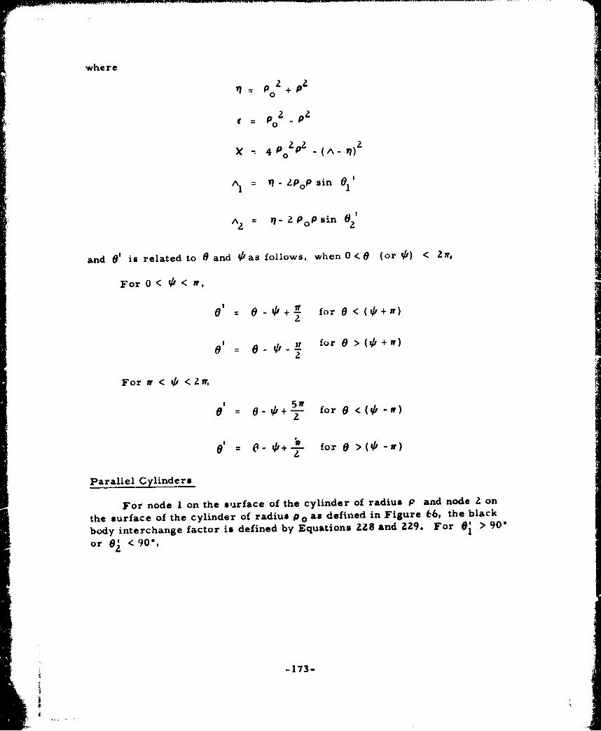
where

€ Po2 P2

0P P

X- 4 Po - (A 17)

A 1 12P.P sin0'

A - ZPOP sin 01'Az = .- Zpo z'

and 0' is related to 0 and VIas follows, when 0<0 (or VI) < 2 7r,

For 0 < 0 < ,

0L 0- + for 0 <(4+W)

0 0 for 0 >(PA+)

For w < ip < 2 ,

6 - + for 0 <(0 w)

0 = 1+- for 0 >(VI-)

Parallel Cylinders

For node I on the surface of the cylinder of radius P and node Z on

the surface of the cylinder of radius p 0 as defined in Figure 66, the black

body interchange factor is defined by Equations 228 and 229. For 6, > 90"

or g o*90",

-173-

E

700 00 % PO d

T T

1 02 0

Figure 66. Nodes on Parallel Cylinders

FI-f- f (f-CA)f (fCa )II 1 d I a8 2I

f f 8 (13- d, A - f8 U-d, A,) +lf,(a-d. f )8 (a -dA 2 )

For 0', <90 <

F - f IE Icos@ 1j- PIIf(- A+ -C. AZ)12 2.Z '' ^0 1A 8(18-- ^30d f8 8

f(j-c) 9- f8('d f8 (3 - 2 )- f 9 (1-d) (29)

+ If 8 (a-d, A,)+ f8 (a -d, A 2 ) -f9 (a-d) - f 8 1-c, i)

+ f(a -c, A f -f(a-c)u dI-19

where the functions f and f are defined as

f , tan - + sin- !-_._in- -I8p z 2PZ A

+ + 2+ + sin - 1"A (T) + (230)

f + + 27 +7) (231)

where

10 VE + p 2 0 ZEp j. CU$t2 2

x = 4P 2

= '? -pZsinO

I I

A " 7 - ?pZ sin 0)

when 0 < V, < 2€ and -v< 0 < r, O9 i. related Lo 1 and 0 as

I¢ - pt• in ik

S= 0 ---- tanE PolI co,-

Cylinder and Skewed Plane

For nodes I and Z, as defined in Figure 67, lying on a cylinder and aplane (which is not parallel to the cylinder). retpectively, the black bodyinterchange factor is defined by

-175-

S --

z E

. 00 PdO

z dl

-7

- y

d /x C

Figure 67, Nodes on Cylinder and Skewed Plane

d 6

p sin, ) -fb

I 1f

(23Z)

+ f 0 (a, e) - f 0 (a, f) dOd7

wherre the function f1 O is given by

G,

10n(A -Z.PAcosO+ )

G2 22 In 0(A - 2ACO 6+ 8+

-176-

a?(A- pcosg)+VJ cos6(pcACos -8) a-z.. I, tan-2 2

1 "P Cos 0) A- ZPACOS-+cos+ 1

G 1 Ocos 0 - G 3 -1 A- PCOSG+ ______ tan-_ ____

p 2 Cos 2 5P 2 Cos 2 0

G 2 Pcos O-G 4 1- A - P cos 0S...4 0 C s- O ta n -- (2 3 3 )

C: " ¢8 W P 2 cos 2 0

where

z

G = /33 + 2p coB 0 (a 3 + 2.0cos 0 cot q) - •2 COB cot lk

G2 - 81

2/33 + 2 cos0 (a3 + 2 P cos cot 4)- 8 cos 0 cot4t

G (a 3 + 2,0cosz OcotP) -Y 3G3 =8 2= a

2 81

= 1 (a 3 + 2o cO 2os Ocot 4) - Y

t,4 =82 - 81

S= (E - Psin 0 + ZI cot ,)Z

SII

C= (cos 0) + T

8z = 81+ (Z1 _ )

-177-

and

03 p _z Coz 0

z(- z 1 ) (Za2 pcos0 +p 2 V3 -+ vf 4 rcos0)

5 p2 Cos2 0) cot/Cos [0 - Z) (E - psin6) 2

c ot - --(,cosO)

-r + Zl ( Z + ZP (E +Z1 cot qt) sin 0- 2zP

a lzi (a. + Pcos 2 OI7) - fapcos2'

-(E +Z I cot 41)sin 0+ P [8- 2 Cos 2 ) cottk.J

3 a - p2 1cos 2 0 1 ( pCOS2 0)(az P+8

[(E + Z 1 cot4)sin o- Pf(E -P sinO)(4 - Z1) p2 0

cot -p

- Z.Z (Z p) [2 2C O) cotob

-178-

Cylinder (Internal)

For the case of two nodes lying on the inside of the same cylinder,as defined in Figure 68, the black body interchange factor is defined by

z

-PdO1

-a 11by

OA OC 00

x

Figure 68. Nodes on Cylinder (Internal)

00

F -iI f 1l (b-c, OB) - f (b-c, GA)12 -WA fI

G1c

+ fll (b-d, GA) - flI (b-d, GB) + f l (a-d, GB) (234)

"f fl (a-d, 9 A) + f1 (a-c, GA) - f1 1 (a-c, OB) d1

where the function f1 1 is given by

-179-

fl(A -'^))= 8+ 4P4 tan

8.e

__ A9 1) tan1 _ _____(235)

2 Psin

Plane and Sphere

The black body interchange factor between node 1 on a plane and node2 on a sphere, as defined in Figure 69 is given by

d b 2 02

F. 1~ P Il ( sin 41(E - P 1)( P) d~dq1idx dyA f ff (1 2J+ E(2 +(y1) 2 2 PC)2 1d1

C a # X1 1( (236)

where

17 = sin 4&sin0 sinq + cos ; cos

c= xsin I1cos O + E17+ y (sin Visin 0 sin 0 - cos V sin )

Equation 236 is not integrated analytically because the resulting IBMcompution routine is more complicated than the case wherein all four inte-grations are done numerically.

Internal Symmetrical Radiation

For the case where a node is defined as a ring around some symmetri-cal body, computation of the black body interchange factors is greatlysimplified. The black body interchange factors between the various nodes ofthe sphere-cone -cylinder configuration of Figure 70 are given by thefollowing equations.

-_ 80-

b

NOTE'r IS 1,AASURED IN yz PLANE

Figure 69. Nodes on plane and Sphere

NODan- NOaNDni

Figure 70. Sphere -Cone -Cylinder Configuration

For nodes on a. cylinder,

F(n, n') 40 ( nl If12 (an - an -I flZ (a~n - an')

(237)(a- - a) - fI 2 (a 1 - aL-) J

where

For nodes on a sphere,

F(mOmm') - (cos - -co ,39)

4 p2 (

, n - 182-

whr

-. ..... .. ....

For nodes on a cone,

•-sinFlG C ' = (b)117(z-b -b

2 b_2 .12 (b b -1)(b I)-e (I• bb+bn

where the function3 by

S£13(•':) =1 [(•-e)Z +(I tan) ~ VI+ tant(41

[a(9 + ta O\ ± tan

For a nod f on a sj.here to b node 1n a cylin,.•r,

1= -1 1a I 1(cos - cof)

n) ,(cos - cos ba

+ H-

•i+ 13 (an 1re (P 1 tan' tre(241)

_~ __

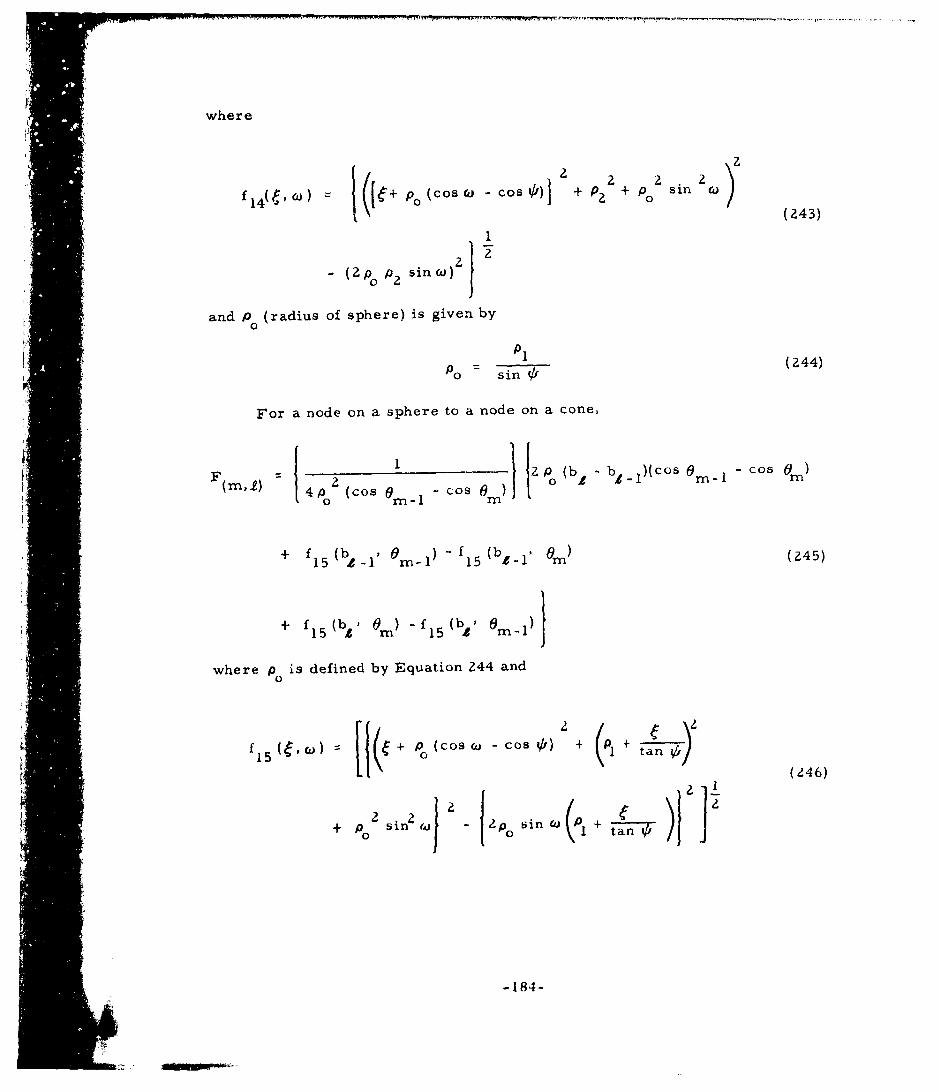
where

z

f Po (Cos - cos) + P + po sin(243)

- (Zp P. sinco)j 2

and P (radius of sphere) is given by0

P1Po sin (1 (244)

For a node on a sphere to a node on a cone,

1 2 1 2P (b, be ,)(Cos r -cas )

4(mn,) 14P (Cos 09~ cos 0- to Cos Ornm

+ f (b ) - f (b O)15 1 1 i-1 15 4-1 ni(245)

(b - (15 Mn 15 'e* r

where p is defined by Equation 244 and

f + a (Cos CU - Cos 1A) + + ta )

(246)

+ 2 sin% " -, 2psinCO (P +)-4tan-

-184-

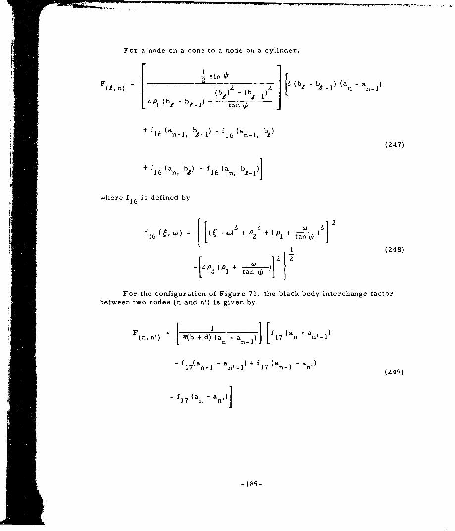
For a node on a cone to a node on a cylinder,

s sin•s n b (a aF(1,n) Tb) (b Ie n n-lS12 (b b be i)

(2,n) [2] (b2 - b2 _1) + (b) -bI -

L etan /

f (a b) - f16 b()16 n-1, 2-1 16 n-1,

(247)

+ f16 an, b) f16 (an, b 1)1

where f is defined by16

f16 (2,o) = [(1 )2 +j+(p 1 + tan Vj

1 (248)

" 2/p (pl +tn

For the configuration of Figure 71, the black body interchange factorbetween two nodes (n and n') is given by

F = f (an - an 1(n, n') b+n n-

"17 (an-I aW- 1 ) + f1 7 (an-1 an.) (249)

S17 (a n I

-185-

where f 17 is

17b I bb bba

1 + d tan /,2--- 2 btanv +d

-I d -Id+ d -Z +b tan- d d • tan - (Z50)

1 ( Z:2 + b2 ) (e?. + d2)

+ +b + d

an-

Td

kNODE n' --NODE n

Figure 71.. Rectangular Box Configuration

-186-

DATA OF ASME PAPER 56-A-144

The configuration factors for various cylindrical shapes presentedhere were published by H. Leuenberger and R. A. Person in Paper56-A- 144 of the American Society of Mechanical Engineers (Reference 24).

Directly Opposed Parallel Disks

1 UPPER DISK2 LOWER DISKr RADIUS OF UPPER DISKR RADIUS OF LOWER DISKa DIFFERENTIAL SECTOR OF Ib DIFFERENTIAL ELEMENT OF aP DISTANCE BETWEEN b & DISK AXISL DISTANCE BETWEEN DISKS

Fb +P RZ + L2) 7Z (251)

F =F 1 1 + R+ L R + L 2 22a, 2 12 2•r 2 + 2- 24 22

when R Rr,2L2 2L2

187 -

whn

* The limiting values are

L--0 12 1 R> rF12 = R 2/r2 R < r

L--O F0 =12 0

FR- 12 =0

F Rz F 21

r --- 0 F12 R 2 /(L + R

roo F12= 0

Cylinder

Cylinder

"1 TOP OF CYLINDERaBOTTOM OF CYLINDER

3 3 CURVED SURFACE OF CYLINDERIR RADIUS OF CYLINDERLL HEIGHT OF CYLINDER

On soa DIFFERENTIAL VERTICAL, STRIP OF 32b DIFFERENTIAL ELEMENT OF a

z DISTANCE BETWEEN b & 2

2 2z + 2R Z

F b, -12 + 4 Z R (253)

L 2 2 23, I + LR Z+211 - (L Z) + 2R (254)

Z.R /ZZ + 4R- 2 R r(L -Z) 7 + 4R 2

(L =F2 1 V -2 -L-) (255)-188

.:. i m a DFFERNTIA VERICALSTR18O8-

F 2 = F 3 2 2--56

F a, 3 = F - + (257)

The limiting values are 1

L - oo F 1 3 = 1 Z--0 Fb, Z 2 2 2F 3 3 = 1 1 L L+ 2R

,iL -- 0 F 1 3 0 b, 3 2 2R Z R +

R 13 = 0 2 L 4RF 3 3 = 0

R ýoo F13 = 0F3 3 = 0

R F = 1

F 3 3 1

Directly Opposed Parallel Annuli

1 INNER DISK CONTAINED BY TOP ANNULUS2 TOP ANNULUS3 INNER DISK CONTAINED BY BOTTOM ANNULUS4 BOTTOM ANNULUS

l r INNER RADIUS OF ANNULUSR OUTER RADIUS OF ANNULUSL DISTANCE BETWEEN ANNULIRZ>rl, R4 > r 3

44 3

14 r (+ R 42 + L )

14 2 2 2

+ -4 3"2 (258)

-189-

F [y/R2 + L)- (Zr Rz)

F24 =(R 2 2+ r32 2 2 2)

-/(R + R + L2)2 (2R2R4)2 + 1(r + R42 + L') (2r R4 )12 4

( (+ r 32 + L2)2 - (2rlr 3 ) 2 (259)

When R. = R and r =r 3 = r,2 4 1 3

FiI4-• - R + L -'4( + L (260)

14 2 2 + 2 R R 4 (26)r r R2

24 +(261)

The limiting values are

L--. F =014L-.- F24 =0

L---0 F =0 r > r14 3 1

2r

3= I 2-• R4 > r>r > r 3

r1r

2 2R - r 3S 2 3rI>

R14Ir

: -190-

L-0- 024 > R or r > R

2 22 r3 >~~

R 2 2 R4 > R2 > r3 > r1

1R4 > R and rI>34 2

R 2 2

2 R 2 > 4 and r 1 > r3R 2 - r 122 41 3

2 2 2r r +

1 1 32 - 2 2 2 2

r + r + L) - (2r 3 rI2

2 2 2 1r -R +L

4

2 2

R 2 r2

r 0 F'114 2 2 2 2

R4 r 3

rL + R4 L + r3

-191-

Cylinder and Annulus Contained in Top

I DISK CONTAINED IN CYLINDER TOPR z! ANNULUS IN CYLINDER TOP

ri3 BOTTOM OF CYLINDER

L.4 CURVED SURFACE OF CYLINDERr INNER RADIUS OF ANNULUSR RADIUS OF CYLINDER

4 L HEIGHT OF CYLINDER

IN

+ L4 2 r + ýL ) ~(ZRr)2)j

(262)

"F - [ R + L R L- )2] (2 6 3 )

Si [ i-R2 Lz

14 2i2 4 + 2

!i,| |iThe limiting vahues are

F-=_ 14 ( 4 + L2)

-192-

Two Concentric Cylinders of Equal Radii (One Above Other)

"-1 CýR I CURVED SURFACE OF TOP CYLINDERLl CURVED SURFACE OF BOl IOlv CYLINDER

i $ TOP OF CYLINDER I.4 BO'I"IOM 01- CYLINDER 2

R RADIUS OF CYLINDERS,L1 lHEIGilT OF 'lO1 CYLINDERL,) HEIGHi'r OF BO'ITOM CYLINDER

S, L•

S+ +ZL LF [(L ) + L2R 1 2 2 L 2

L1 + 2 (264)

2] + L2F4 -2+ L L ++ L2 L + L

F 2+ i____ Il 2)

Swhen L L2 L,

F 1 4 / '+ L-2.3 4+ L 2 (266)14 2 R2

FL 4+ - (267)

122R /4+R22/+ R

-193-

The limiting values are

2L2 + 2R 2 L21I-' 1I4 = - 2R-

2RfL22 4R22

2 2

S2 L 2 +2R2 22

2R L + 4R2

Two Concentric Cylinders of Equal Length (One Contained Within Other)

I CURVED EXTERIOR SURFACE OF INNER CYLINDER2 CURVED INTERIOR SURFACE OF OUTER CYLINDER3 BOTTOM ANNULUS CONTAINED BETWEEN 1 & 2

4 TOP ANNULUS CONTAINED BETWEEN 1 & 2

R RADIUS OF OUTER CYLINDERr RADIUS OF INNER CYLINDER

L HEIGHT OF CYLINDERS

a DIFFERENTIAL VERTICAL STRIP OF 1

b DIFFERENTIAL ELEMENT OFac DIFFERENTIAL VERTICAL STRIP OF 2

d' d DIFFERENTIAL ELEMENT OF cz DISTANCE BETWEEN b & 3W DISTANCE BETWEEN d & 3

1 -1 W2 2 R 2 2- (L W)2. R2 +

F i - cos + CR +d,I R + (L W) 2 + R2 2

2 2 2W W2 + R2 + r -1 r(W2 R + r2

-- r y ' ..... COB z RW....z .~ al

2 2 2r [2- L{ -) -!- R (+r

(L W)2 + R + rz8)

-194-

Cos-1 r [(L-w)2 -W- + r 1 LCO! R[(L W)2 + R -r 1 r

i!!!. (l - ) +" R L W + zR.2 (269)di, 2 R 2 2 (,FR =2L W'+2 (RL4-+ (L - W)2

1 [2r 1- 2 R 2 - r-1 2 L -_ 2an + tan L-W + - sin - 2

2 2W 2 22 2 4(R -r2)+ E2 (R' - 2r)

W + 2R s-1 R2 2 W2 2 2

R4R- +RW4 2 W + 4(R - r

2 2• 4(R 2 - r2) + (L2 (R2 2r2

(L - W) + 2R s-1 R.

R4R(L+-LW )2 (L - W )2 + 4(R - r z)

F (Fd + FP ) (270)d,3 2 dI d,2

*Evaluated with L replaced by W

2 - 2 2 z 2 R2 2F 1 -1Z -R +r Z + +rXb, 3 fn R2 -r 2 r (271),i~~ iii R- --r (Z2 +z RZ 2 -2•

+ R + r . -4R r2

2 2 2S-1 r(Z - R +r) - os-r

R(Z + R -r)-I

F b,Z 1 l (F b, 3 + F b,4 ) (272)

-195-

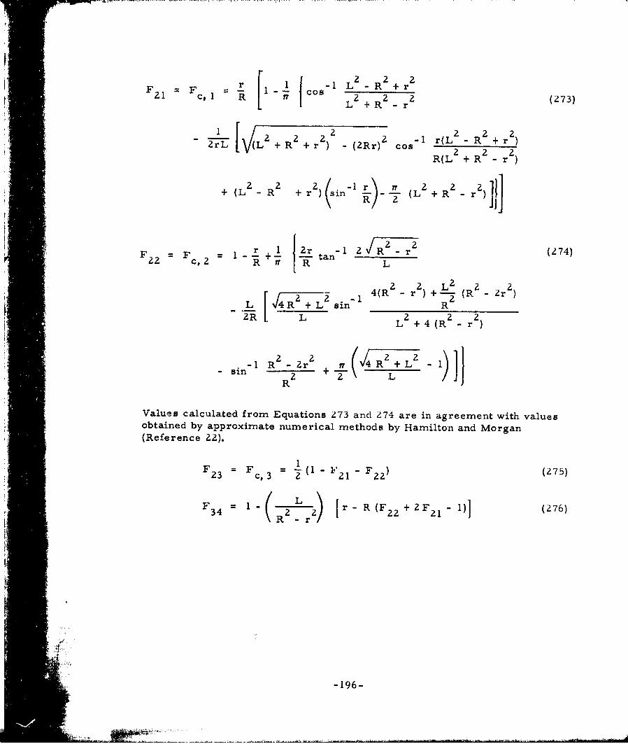
F r [l coo L -R +r r21 C, L2 R 2 2 (273)

2 2 12 2- r(L- -R ) + r2rL[(+R+r)- (2r) CoBs

R (L2-- -R-2 - r

+ (Lf R 2 + r 2(in- ) r . (L 2 + R 2 - )

r -1 R r-r(74

22 c, R1 Ri- +1 2- tan- 2 R 24

2, 2 LR 2r R

I4(R IrI + L2- - Zr

-L 4 + sin RR• . L 2 2

L + 4(R2r

S 22IIn - r1 4+ - )J 7

i~mR

ZR L L2

Values calculated from Equations 273 and 274 are in agreement with valuesobtained by approximate numerical methods by Hamilton and Morgan(Reference 22).

F =F 1 ., F(27 5)23 c,3 2! F 2 2

F3 4 =1-~2 [r- R(F 2 + 2F2 - 1)1 (276)

-196-

L/R

2

0.8 .1

UV 0.4-

0. 2

00 0.2 0.4 0. 6 0. 8 1. 0

r/R

Figure 72. Form Factor From Outer Cylinder to Inner Cylinder

1. 0L/R

r\0. 8 4

2

~0.2

0*

0 0. 2 0.4 0.6 0.8 1.0r/R

Figure 73. Form Factor From Outer Cylinder to Itself

- 197 -

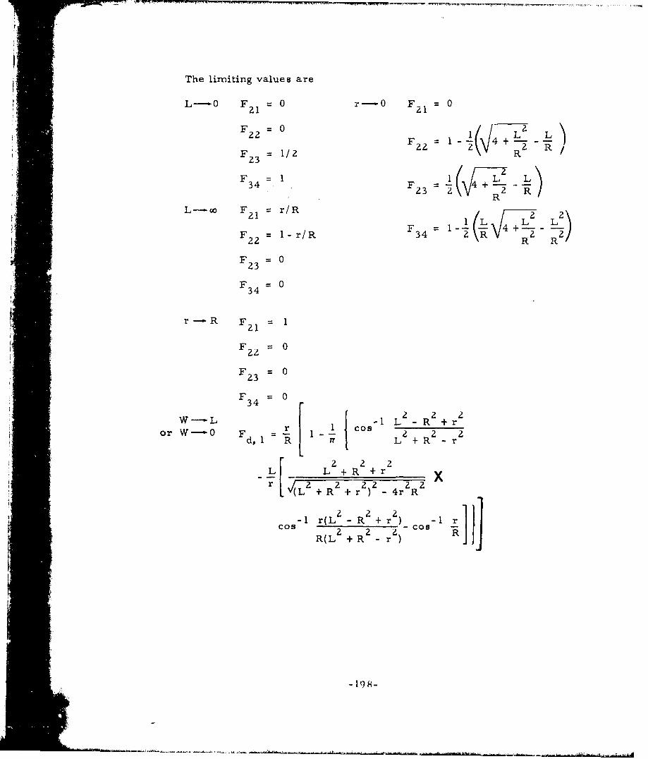
The limiting values are

L--0 F21 -0 r--0 F21 0

F22 0 4 2

F34 1F (ý + L -• L

3 1/ F3 = RL34

F-2 3 (2Q 2L- oo F r/R iL L 2

F =0

34

r--R F =1

FZ = 0F220

23

F 034 0

W-L2 -1 2 L R2r 1 cosorW-0- 1 -- 2 2

d, 1 R IT L +R -r

2 2 2_L L + R +• r- f( - +Rý+ r 4r xCs 1 r(L - R 2 + r 2 )_ -2 r

2 2 Ro2( +R-r2)cs1r}

-198-

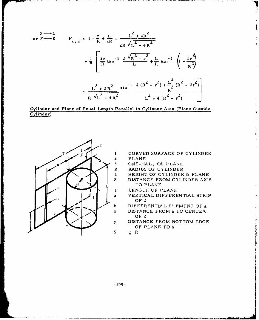
7-L r L L + ZRor 7--0 F I " +

(1 R 2RZR 1 L+Z JILT+ 4 R

I -I Z -._ r LL + t sin

2RR 2r-l

2L RZ r (L- + 2Rz sin' R 2R z • ( "zz

R 4 7+ 4R'- L2 + 4 (R - r )

Cylinder and Plane of Equal Length Parallel to Cylinder Axis (Plane OutsideCylinder)

I CURVED SURFACE OF CYLINDER2 PLANE

x 3 ONE-HALF OF PLANER RADIUS OF CYLINDERL HEIGHT OF CYLINDER & PLANES DISTANCE FROM CYLINDER AXIS

R .TO PLANEST LENGTH OF PLANE

a VERTICAL DIFFERENTIAL STRIP00, OFz

b DIFFERENTLAL ELEMENT OF ax DISTANCE FROM a TO CENTER1~ OF 2y DISTANCE FROM BOTTOM EDGE

OF PLANE TO bS R

-199-

W ill, I I_ _ _

FR 2 2jCos-1 2 S + R2 2 2 S2 + +

SC - (L y) -S -Ix R + R +(L I 2 + 2 + o 2 S2 (277)

S2 ++ + -x -R

2 2[ +R

Cos -, 2 22 .22(77

+S+x - R + + R/(, + 2 2 2 2

2 2 2 2z•' Cos ...( )

SR'+x (y +S2 + x 2L- R 2

s xL-y)2+S2+x - R2 + 4(L-y)2R2

-1 R [ (L-y)- S2- x2 + RZ]

+ Cos1777 L~Y~S2+:R2

+) + -1- R

S 2+x1] _____ __

SR 1os I L 2 - S - x2 + R2

a, 1 S + x 2 + + -

R-L [/('+ +S +x + R ) +4L 2 R2 XZIL 2 S 2 2 2

Co- R (L2 -Sz 4 R)

-Sz -+72 (L2 + S 2 + x2- R 2

2 2 2 2 -1I R

+L-S -- +R+ )

+ (L - S - x + R ) sin" V- + IR

S1S22+2x2

- +S + x (278)

-200-

!117

F 1F 3 1 f 1Fa,1dx (279)

The limiting values are

y -- o L0 2 2 R zor y- L F SR lL- 1 Cos - - × +b,1 + x IX L +S +x -R

LL +S +x + 2-•L2 + S' + x' R') + R

-1 (L 2 2-RL-S - x +R)."F: SS + x 2(L 2 +S + x - R 1

- COS- Rs-Cos

+x]]

L- 00 F RS R-0 F =0b, 1 S2 + 2 b, I,. S +x;IIF -=0

RS a, 1F

a, I =S + x 0

21

F F tan- I T T 0 F F where21 31 T 2a 21 a, I

'a, 1i

L-0 F, =0 evaluated atb, 1 x= 0

F =0a, 1

F21 0

JJs--b00 FD, 1 0

! llql .F -- 0a, 1

F =0

-20 1-

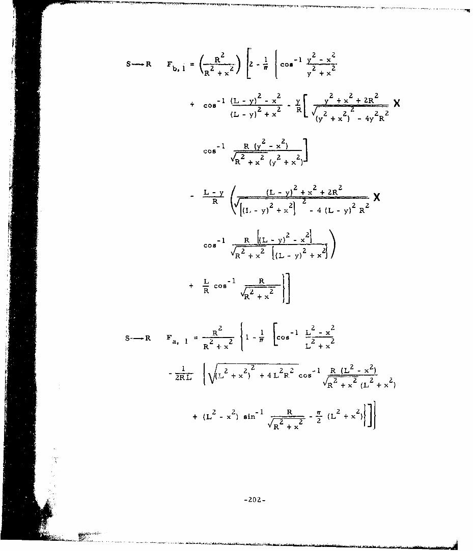
R- x

S--.R Fb, -1 2.i- coo 2 2R + x Ly +x

2 x2 y2 2 2I (L - +x x + 2R) y+ Cos) 2 R (/ .. .. .(b - y + x + xZ~ 4y2R

2 2-1 R (y x)Cos /R2 J

R + x (y + x

L ( L - y)2 + x + 2

R R2 - 4 (L 2 R)2

+) + x Y

22x

R RLS-R a F- • L L+x

22 22 -1 R2(L-x)

2RIK +x) + 4 L cos 2 + 2 +IR+ + x- (L?" +x

L sin L 2 +x

-202-

Cylinder and Plane of Equal Length Parallel to Cylinder AKis (Plane InsideCylinder)

w II I VERTICAL INNER SURFACE OF CYLINDER2 SIDE OF PLANE FACING I3 ONE-HALF OF PLANE

a- 3 IR RADIUS OF CYLINDERL HEIGHT OF CYLINDER & PLANES DISTANCE FROM CYLINDER AXIS TO PLANE

(TAKEN POSITIVE AS SHOWN)1 Ia VERTICAL DIFFERENTIAL STRIP OF Zx DISTANCE FROM a TO CENTER OF PLANE

0*11-1 RS+X - R-s-

F tan L + tan L

x (R2 S-2 -x 2 ) j( -R -s X) +L ]

4(x2 +S2) (R2S2 +x)2 +L L

r 2-1S-x R-S -I&~ S+x -LSZ zif

xL /R 1? R S ++ L

Cos + Cos 2 2 2 2 2 2/7 2 I:Tx-

+ •(L2+Rz +S +x)- 4R (xZ +S) dX

cos' 2R 2x 2 +S (R - S 2- x 2- L )+x(R 2S +x2 + 1,zR 2- S

1 F Vs2 +x 2x 2 Rt2 + x) - L2

(280)

-203-

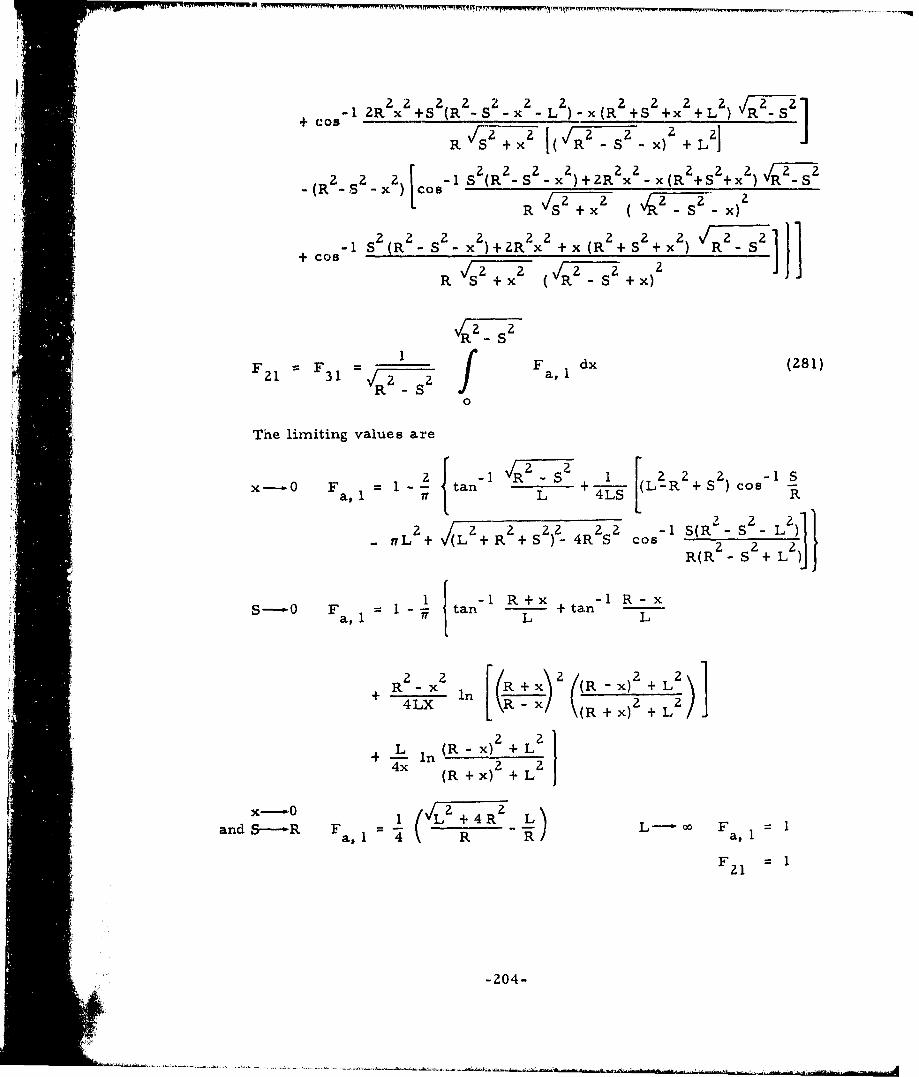
1 2 x 2 2S 2 (ZS 2 -x 2- 2 xR 2_+S2_2x 2 +L 2 2R S+ CosB- ZR x +S (R -S -x -L )-x(R +S +x +L ) -s2

R LZ_ •I+2o'o sS( 2 -S2 2 22 z)2 2 2-

R- Sx )+2R x -x(R +5S + x RS(R -S -2 xx)CO

22 2/S2+X 2 S2 2 2 21)

+CS-1 S (R2- S2-x 2)+R2Rx 2+ x(R 2+S2+x)2 RS?

VC-2 7'T2 ,2 2 2 IR S +x ( R s + X)

R -S1II

F1 IF F adx (281)F21 = 31 /R2 2 a,1

R -S J0

The limiting values are

2C 2 [ ý+a,1 1F - +-t-S LRZ + S2 ) cos"

x. a, F1ta L 4LS L+Z1+2 / 2 22 22 -1 S(R 2- S 2- L

,- L + +R + -4Ros C2.2R(R -S +

I -1 R+x -I R-_ x

S-.- F 1 - tan - +tan La,l I LL

+R2-I [) 2 +2)]+i-L i n + - (xR)

4Lx 2

(" + )X + L

!! ! _.I+ L In + L4x ( + x-- i (•L +4 L z

a, 1 (ý +4R R/ L-~ F00 1"and S--"R R a,

F =I

"-204-

Two Concentric Cylinders of Unequal Radii (One Atop Other)

b 1 INNER CURVED SURFACE OF TOP3. CYLINDER

1 z INNER CURVED SURFACE OF BOTTOMz CYLINDERW 3 TOP OF CYLINDER 1

4 BASE OF CYLINDER ZR RADIUS OF 2r RADIUS OF 2LI HEIGHT OF 1

L LZ HEIGHT OF 1a DIFFERENTIAL VERTICAL ELEMENT OF 1

b DIFFERENTIAL ELEMENT OF az HEIGHT OF b FROM BASE OF 1R > r

s4

For

L 1

L 2 (--1) (2 receives no direct radiation from 3)

LI:LL r L

21 + + (2

I4 4 2 L

r rRL + l RR+L2

+ + 2z ) 4 R (283)

r r

-205-

For

i~Li

L [ 2 2 2 2 2 2

S1 -+ + r 1 + 4r2 R - rb, 4 + 4r 2 %/-(2L2 + Z) - R2ZZ

(284)

2 2 2S1sin Z - r2 R +r +(Z+L 2 )-" i-i .... -IJ +. . . ...1. . x2r Vr'L2 (L +Z)J'Z 2r 2)[2

2 2 - L2 21 2 2 + 2 2 2

1 - r - (Z + rL + Z(R- r2)LR -o 2Rr(Z + L 2 ) [L 2 (Z + L2 ) + R 2 - r2]

Z(R - r2 ) 2L 2rr

Ol co 2RrLI

fLFd

LIII L ]

•-" -"---Jo b, 4d

F 14 F = (285)

12 2 (286)FI'=/4 + R2 R - a, 4 (86

-20 6-r'4

/.

The limiting values are

-0: F , -w1 tan- 1 JR " +7•-- ' '... Z, XFb, 4 L L2 + r2+ . 4R2 z/

R(LL 2R7 r 4l

(R2 -r

r- 1

) 2C 2

2 2

Z-0 L 22+Z2R 2 L2VL2 2

"" "R 2 + -_ 4-R]ý) |4

+ L-' L(1 + 2L

adr-.-R F Ll1,4 2 2 RR

2 /1•4 R R

-207-

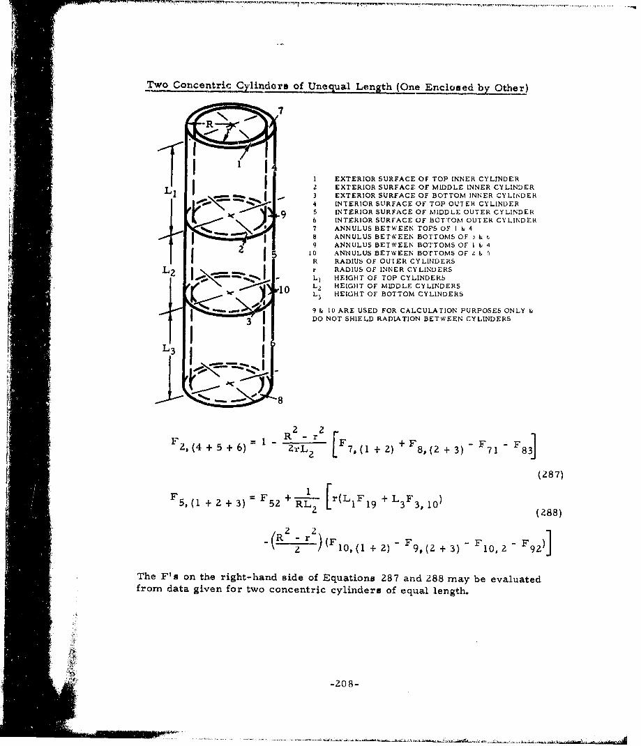
Two Concentric Cylindera of Unequal Length (One Enclosed by Other)

I EXTERIOR SURFACE OF TOP INNER CYLINDERI 2 EXTERIOR SURFACE Of MIDDLE INNER CYLINDERL I • 3 EXTERIOR SURFACE OF BOTTOM INNER CYLINDER4 INTERIOR SURFACE OF TOP OUTIER CYLINDER4 INTERIOR SURFACE OF MTIDOM OUTER CYLINDERSF. 6 INTERIOR SURFACE OF BOT tOM1 OUTER CYLINDER

7 ANNULUS BETWEEN TOPS OF I & 4

b ANNULUS BETWEEN BOTTOMS OF & t€S9 ANNULUS BETWEEN BOTTOMS OF I & 4

5 10 ANNULUS BETWEEN BOTTOMS OF 4 &I IR RADIUS OF OUTER CYLIN4DERSL2 Ir..... r RADIUS OF INNER CYLINDERS

I " - L 1 HEIGHT OF TOP CYLINDERS

1(•Z 1 HEIGHT OF MIDDLE CYLINDERSli 1 L3 HEIGHT OF BOTTOM CYLINDERS

9 & 10 ARE USED FOR CALCULATION PURPOSES ONLYS3 DO NOT SHIELD RADIATION BETWEEN CYLINDERS

• B ~~~L3 ._.q.

S1z88)R 2 2F9, F F93 ]

-- m . ..---- ( - r 8F -2 7 1

2 ,( 4 + 5 +6) ZrL 2 F 7 ,(l + 2) +F ( + 3 )F 71 83

f i- (287)

F (123) F +-. [r(L 19 +L F3 05'1+2 ) 5 L2 1 9 33 0(Z88)

2 10,(1 + 2) F9 ,(Z + 3)1 ,2 -F 9 2 )]

The F's on the right-hand side of Equations 287 and 288 may be evaluatedfrom data given for two concentric cylinders of equal length.

20m8-

DISCUSSION

To permit full utilization of the foregoing tabulated data, a summary ofconfiguration factor properties and a discussion of some useful techniquesfollows (from Reference Z5).

Vi • Reciprocity

The reciprocity relationship for the configuration factor from A toA is

il iAIFl = AzF (289)A1 F12 =A2 F21(29

This relationship often allows a great simplification in the analysis ofconfiguration factors; F 2 1 can be obtained directly from F12 and the areas ofthe surfaces.

Sum Equals Unity

By definition, the sum of the configuration factors to all surfaces seenby a given surface is unity. This relationship is often written as

n m

ŽJF( . (290)n 2

where

m = Total number of surfaces

Yamnauti Modified Reciprocity Relationship

A modified reciprocity relationship, given by Yamauti, is also useful.(A general proof of this relationship is given in Reference 26, p. 336-337).This relationship in terms of the areas of Figure 74 is

S14 A 1 F 32 A3 = F23A2 = 41A4 (291)

-209-

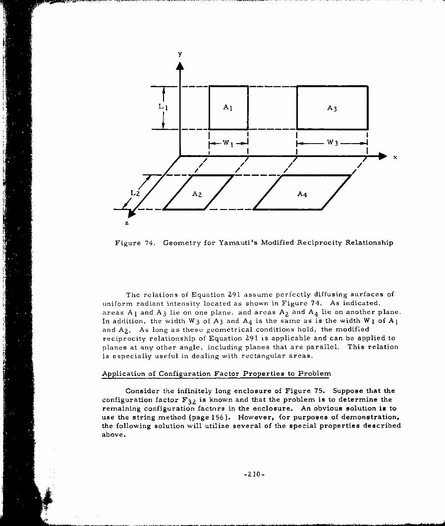
LAl A3 J•1 l i l•" L'•'•• ..... l

V, I III I

'/ /

ZZ 7

2 4

//in /, ,i // // .x

4'-

Fgr 74. Geometry for Yamauti's Modified Reciprocity Relationship

reciproiThe relations of Equation 291 assume perfectly diffusing surfaces ofunif.orm radiant intensity located as shown in Figure 74. As indicated,]•_,ml •:.areas A 1 and A 3 lie on one plane, and areas A2 and A 4 lie on another plane.}iii In addition, the width W3 of A3 and A4 is the same as is the width W1 of A 1

•m••and A 2 . As long as these g~eometrical conditions hold, the modifiedi=•i l••reciprocity relationship of Equation 29 1 is applicable and can be applied to

planes at any other angle, including planes that are parallel. This relationis especially useful in dealing with rectangular areas.

Application of Configuration Factor Properties to Problem

Consider the infinitely long enclosure of Figure 75. Suppose that theconfiguration factor F 3 2 is known and that the problem is to determine theremaining configuration factors in the enclosure. An obvious solution is to

use the string method (page 156). However, for purposes of demonstration,the following solution will utilize several of the special properties describedabove.

-210-

A2

Al A4 2

A3

Figure 75. Diagram of Infinitely Long Enclosure

The enclosure of Figure 75 is symmetrical in that A 1 = A4 and A 2 =A 3 .Because of this symmetry, the following configuration factor relationship can

be written as

F =F41 14

F =F (292)32 23

F 31 31 F 21 F 24

Assuming that F 3 4 is desired, apply Equation 290 to area A3 ,

F32 + F31 + F34 = 1.0 (293)

Using the relations of Equation 292 in Equation 293 yields an expression forF 3 4 in terms of the known configuration factor F 3 2 .

F 3 4 = 1 - F 32 (Z94)

-211-

Once F 3 4 is known, the remaining configuration factors for Figure 75can be determined by the reciprocity relationship. For example, theconfiguration factor F 4 3 is given by

A 3

F =F A3 (295)43 34 4

Configuration Factor Algebra

In many instances it becomes necessary to determine configurationfactors which cannot be found directly from the tabulated data. For examplesconsider the case of a surface A3 , which is perpendicular to a second surfaceAZ, and the two surfaces do not have a common edge as shown by diagram Zof Figure 76. The configuration factor F 3 . for this configuration is desired.As is evident from the geometry of diagram 2 (Figure 76), F 3 2 cannot beevaluated directly from the graphical data.

A convenient technique for evaluating F 3 2 is to consider the flux

transfer between a fictitious source consisting of surfaces A3 and Al andthe area Az. Denote the flux received by area A2 from A(l + 3) as 0(l + 3, 2)-From. this must be subtracted the flux ) *12 due to the source A1 yielding

032 - (1 + 3, 2) - 012 (296)

The total flux leaving an area A which is incident on an area A is given byn m

3JF A(27(n, m) n (n,m) n(97)

where

J = Radiosity or total flux per unit area streaming away from surface nn

Substituting Equation 297 into Equation 296 yields

j33 3 = j( + 3)F(1 + 3,2) A(1+3) - jIF12 1 (298)

Assuming that J 3 = j3( + 3) j1 = 1.0, Equation 298 becomes

F32A3 =F(1 + )A(1 - F12A1 (299)323 1+ 3,2)( + 3) 1 29

S~-212-

Basic perpendicular configuration (for F 2 1 or Fl. use(1) configuration factor graphs)

A 3 F 3 2 = A2F23

3A(I+ 3 )F(I+3 , 2 ) 1AF1 2

A 1F 1 4 =A 4 F 4 1

(3).. = I/2 [A(1+ 3 )F(1+ 3 , 2+4)- A 1 F 1 2 - A 3 F 3 4 J

3

AIF(I, 2+4) A(2+ 4 )F( 2 +4, 1)

(4) =1/2 IA(1+ 3 )F(1+ 3 ,2+4) A3F34 +AIF(12)]

A F -A F3 (3,2+4+6) (2+4+6) (2+4+6, 3)

.1/2 [A( )I F(1+3)F(1+3,2+4) (3+5)F(3+5,4+6)-

1 12 A5FI

Figure 76. Diagrams of Configuration Factor Algebra (Sheet 1 of 2)

-213-

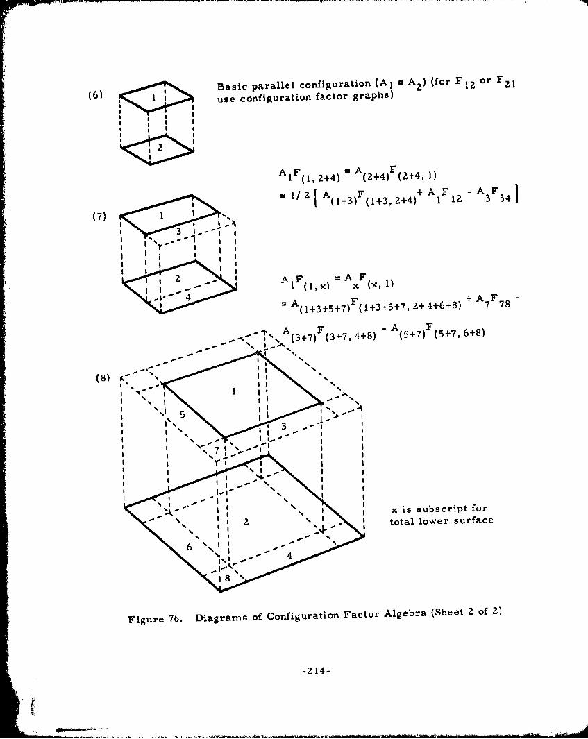
(6) Basic parallel configuration (A1 I A 2) (for F 1 2 or F 2 1

(6) use configuration factor graphs)

B gB I

AIF(1,2+4) A (2+4)F (2+4, 1)

_1/21 A(1+3)F +3 +4 + A 1 - A 3 F 3 4

(7) 9

F F+A

1~ (1, X) x X4

(1+3+5+7) (1+3+5+7, 2+ 4+6+8) + 7F78

* •~ A F -A FA (3+7) (3+7,4+8) (5+7) (5+7,6+8)

(8) K" • %

x is subscript for

- total lower surface

-4 4

Figure 76. Diagrams of Configuration F actor Algebra (Sheet 2 of 2)

-214-

Solving for F from Equation 299 yields32

F3 32 -A (1 + 3, 2)A(1 + 3) Fl2 A 1 (300)

Equation 300 expresses the shape modulus F 3 2 in terms of two shape moduliwhich can be obtained directly from graphical information available in NACATN 2836 'Reference 22).

As a second example, consider finding F 1 4 for diagram 3. Applyingthe same technique as for the first example yields

¶614= 6(1 +3, 2+4) 0 12 -- 34"3Z (301)[

Now, if all surfaces have uniform emittance, Yamauti's modified reciprocitytheorem can be applied, yielding

014 = 0 32 9523 = •41 (302)

Substituting Equation 302 into Equation 301 and combining terms,

04 = [0(1 + 3, 2 +4) IZ 534 (303)

Equation Z97 is now substituted into Equation 303. The resulting equation issolved for FI4 This operation gives

14*

F 1 4 =AF (+ 4 )A(, + 3 )F A 1 - F 3 4 A3 (304)14712~ .2+4 +3 121 34]

Equation 304 is a relation for F14 in terms of configuration factors which canbe evaluated graphically.

A similar procedure can be used to derive the configuration factor foralmost any configuration in terms of configuration factors which can beevaluated directly. A number of the more common cases are summarized inFigure 76, which was obtained from Reference 26 (Table 38).

Finite Configuration Factor Conversion

An important technique for the evaluation of finite-finite configurationfactors is called the area weighted method. Briefly, the finite-finite

-215-

*r9n ,Fh',

configuration factor can be obtained from a knowledge of the differential-finite configuration factor at every point or, as in this method, at certainwell chosen intervals.

Recalling the bacic equation for a finite-finite configuration factor,

F 1 2 C= A j JI S 2 dAldA (305)1 2 S 12

If A 1 is relatively small, the kernel (cos 61 cosr 62 /S 2 ) of this integral ofthe above equation is effectively independent of dA 1 or essentially constant andcan be removed from the integral when integrating over A,* Thus

F AA - 0 " s 0 dA. (306)

which is the same as

AA-AA11 - Az) 1 (dA 1 - A 2 ) (307)

The quantity AA 1 is a smaller finite area that forms some part of thelarger area Al. The configuration factor F(dAl - A2) is taken from the centerof AAI, to the whole of A 2 . By summing up terms such as given in Equation307, the total shape modulus FlZ is obtained.

F = ( - A (308)

Al

-216-

CONFIGURATION FACTOR DEVELOPMENT

IBM 7090 PROGRAM (GEOMETRIC CONFIGURATION FACTORS)

An IBM 7090 program (Reference 27) which calculates geometricconfiguration factors is now in final preparation. The program is limited tothe calculation of the geometric configuration factor between two planes whichmust be parallelograms, including the special cases of squares, rectangles,and rhombi.

The method of calculation is a numerical approximation of the integralform of the configuration factor equation from a plane in space to any otherplane. Under control of certain input data the two planes are divided into anumber of incremental areas. The expression for the configuration factorfro-n an incremental area in plane 1 to another in plane 2 is

i| i Cos 0 Icos 01AA•

F 1(309)(dA 1 AAz) =1 2 r

where

o• = Angle between the normal to plane I and line connecting centerpoints of two incremental areas

02 = Same angle for plane 2

AAZ = Incremental area in plane Z

r = Length of line connecting center points of two incremental areas

This calculation is repeated for all the incremental areas In plane 2,and the summation of these is the configuration factor from the incrementalarea AA, to the total second area. (Note that the calculated individualF(dAI.AAZ) takes the form of a differential area to finite area configurationfactor. This is calculated from the midpoint of AA 1 , and is assumed to bethe average over AAI.

The foregoing process is then repeated for each incremental area inplane 1. An integrated average of the configuration factors from all the~A 1 to A?. is equivalent to the configuration factor from plane I to plane 2.

-2 17-

W- MR R W I

UNIT SPHERE METHOD (DIFFERENTIAL-FINITE CONFIGURATION FACTOR)

An extremely useful method for the development of the differential-finite configuration factor is known as the unit sphere or solid angleprojection method. This is discussed in some detail in Reference 26(p 294-298).

Briefly, it can be stated that the configuration factor from dA to A.,in Figure 77 can be obtained as follows: 1

1. A hemisphere is drawn over dA of radius R.

2. The area A ' cut on the spherical surface by the solid angle fromdA to A2 is obtained by central projection.

3. The projected area A ' must then be projected once more bynormal projection to the plane of the radiating surface dA Thearea of the second projection is A in Figure 77.

4. The configuration factor F(dAIA,)is given by the ratio of A." tothe area of the circle. Thus,

A"F 2

(dA1 -A 2 ) ) -R2 (310)

It can be seen that A2 need not be a plane surface as long as theperimeter of the surface is defined (i. e., A2 could easily have been concaveor convex and the same value of F(dAI would have been obtained).i|..d, I - A2)

To determine the configuration factor from a finite surface A1 to afinite surface A?, the surface A1 must be divided into small areas of equalsize and the unit sphere method must be used for the centers of every one ofthese areas. The average of these is the finite-finite configuration factor F 1 2.

The unit sphere method is often useful when the other methods of con-figuration factor analysis cannot be readily used. However, it is a somewhattedious method. There are several ways in which to attack the problem:

1. Descriptive geometry. This is essentially a "brute force, " handcalculation method, which employs ordinary descriptive geometrytechniques.

2. Mechanical integrators. Several mechanical integrators have beenbuilt based on the unit sphere method (References Z2 and 29 through32). These usually require the use of models because they areemployed by tracing the outline of the shape under consideration.

i-218-

/ [

//

/

d~fl

Figure 77. Diagram of Unit Sphere Method forDetermining Configuration Factor

-219-

S- t~a.

3. Photography. Considerable work has been done at the University ofCalifornia at Los Angeles and elsewhere, based on a point sourcelight being placed in the center of a milk-glass hemisphere. Amodel of the area A2 is then placed inside the hemisphere in theproper position with respect to the point source dA 1 . It isprojected by the point source lamp as a shadow to the milk-glasshemisphere. When this hemisphere is photographed from aconsiderable distance, the ratio of the shadow of the model areato the area of the circle representing the glass sphere is theconfiguration factor (Reference 28, p 214-215).

[[

-220

DISCUSSION OF ASSUMPTIONS

When configuration factors are determined, the basic assumption ismade that the thermal radiation involving these configuration factors existsin diffuse form. The complications produced by an attempted analysis of apartly diffuse, partly specular radiation problem are so great that asatisfactory method of analysis for this condition has not yet been devised.

-221-

;,= ,,

Section VIII

EVALUATION STUDIES

This section of the report is concerned with the variables whichinfluence satellite shell temperature and their effect on the cyclictemperature during each orbit revolution. Each parameter is independentlyvaried by choosing various values within a realistic range of values. Theevaluation studies point out the thermal problems associated with spacevehicles and demonstrate the necessity for a large amount of analyticalthermal prediction work required during design of a space vehicle.

These evaluation studies were completed through use of the IBM 7090program, "Program for Determining Temperatures of Orbiting SpaceVehicles" (Reference 33). This program is also discussed in Section V ofthis report.

NOMENCLATURE

a Earth albedo

e Eccentricity

h Orbital height, mi

i Inclination, deg

Q Internal heat load, watt/sq ft of surface area

* S Solar constant, Btu/(hr)(sq ft)

a Absorptivity

a/c Ratio of absorptivity to emissivity

* •Emissivity

w Mass, lb/sq ft of surface area

VARIABLES SELECTED

The variables that were considered are those listed in Table 6. Simpleconfigurations are used in evaluating the effects of the variables on the cyclicsurface temperature and include a rotating sphere, an earth-oriented flatplate, an inertially oriented flat plate, and an eight-sided, earth-orientedprism.

- : :: -- •-Z23-

IpEVIOUS PAGEn

:1 i i i i

Table 6. Study Variables for Rotating Sphere

Variable Unit Variation

Orbital height Distance from planet, 150 to 2000miles

Orbital plane Inclination from plane of 0 to 80ecliptic, degrees

Surface finish Ratio of solar absorptivity 0. 1 to 20. 0to emissivity

Internal heat Watts per square foot of 1. 0 to 20.0load surface area

Mass Pounds per square foot of 0. 25 to 10.0surface area

Solar Constant Near earth solar constant, 433 to 453Btu/(hour)(square foot)

Albedo Earth's albedo 0. 2 to 0. 8

ROTATING SPHERE EVALUATION

Variation of Orbital Height

The cyclic variation in temperature for a rotating sphere is shown inFigure 78 as a function of orbital height. The orbital height in miles wasvaried from 150 to 2000 miles. The fixed parameters for the sphere wereas follows:

Absorptivity a 0.7Emissivity I 0.5Mass wo 1.5 lb/sq ftEarth albedo a 0.35Solar constant S 443 Btu/(hr)(sq ft)Orbital inclination 1 33.0 deg

The results point out the influence of increasing height on increasingpercentage of time in sunlight and the influence of decreasing earth-emittedand solar-reflected energy with increasing height. The maximumtemperatures for the 150- and 500-mile height are similar while themaximum temperature for the 250-mile orbit is higher, and the peaktemperatures for the 1000- and Z0O0-mile orbits are lower. Due to the

-224-

0 00

-Z4 0

c) N nb

-4

r-'-V

0

w wz 00

00-

4.)

CDC

00 N

-225-

choice of fixed parameters, the time in direct sunlight is being opposed bythe reduction in energy from the earth as the height increases.

The orbital period, percent of time in sunlight, and earth emitted formfactor are listed in Table 7 for the various orbits.

Table 7. Variation of Orbital Height for Rotating Sphere

Orbital Height Orbital Period Sun time Earth-Emitted(mi) (min) (percent) Form Factor

150 88.89 57 0.37250 92.17 58 0.33500 100.52 61 0.27

1000 117.92 72 0.1992000 155.4 100 0.127

Variation of Orbital Plane

Using the same parameters as for the orbital height study and holdingthe orbital height at 250 miles, the effect of orbital plane on cyclic tempera-ture variation was investigated. As shown in Figure 79 the inclination of theplane of the orbit to the plane of the ecliptic was varied from 0 to 80 degrees.Also, the year day from 1 January 1961 was chosen from the data in Figures80 through 84 to give the maximum sun time for each orbit plane.

The results are as expected. The increase in sun time with increasingorbit plane raises the mean temperature and reaches a maximum when thevehicle is in the sun 100 percent of the time. The effect of launch day can bedetermined through comparison of the curve for 250 miles (Figure 78) com-pared with the curve for 33 degrees (Figure 79), because all parameters arethe same except the year day.

Variation of Surface Finish

A primary consideration in any space vehicle temperature controlsystem is the external surface finish. The amount of radiant energy re-ceived and the amount of heat radiated to space are direct functions of theexternal condition of the surface. For some space vehicles, wherle theinternal heat loads are low and the equipment temperature tolerance fairlybroad, complete control can be attained by the selection of the properemissivity and solar absorptivity combination.

-226-

&

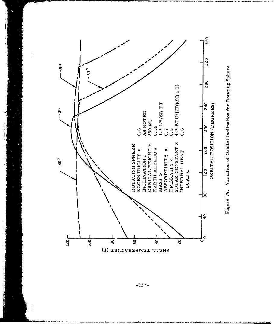
- 0

odo,

000

H Nn

Iz HH~

0 0Zo .,I~

z Ci2

zC

000

w 04

co %0

(a 0uiuaw j 0 0 i~0

In the parametric study described here, the cyclic temperaturevariation was calculated for various combinations of absorptivity a andemissivity f, with no association given to specific materials or coatings.(Unfortunately, although there are several coatings that have desirablethermal characteristics, these materials do not appear too practical forspace application.) The same fixed parameters for the sphere were used.

The results of the study are shown in Figures 80 through 8-. In eachplot, solar absorptivity was held constant but en-issivity varied over a widerange. To point out some of the trends, it is helpful to look at Table 8 wherethe a/( ratio is tabulated along with the maximum and minimum temperatures.

Table 8. Variation of Surface Finish for Rotating Sphere

Solar a/, Temperature (F)

Absorptivity Ratio Maximum Minimum

0.1 0.1 -81 -960.1 0.125 -75 -910. 1 0. 20 -59 -750. 1 0.33 -33 -500.3 0.375 -14 -600.5 0.5 13 -580.5 0.72 4Z -320.1 1.0 53 360.5 1.0 74 -21.0 1.0 93 -381.0 1.11 104 -281.0 1.25 117 -150.7 1.40 120 181.0 1.43 133 -40.5 1.66 130 520.1 2.0 126 1090.5 5.0 285 2060.5 10.0 399 3241.0 20.0 576 434

As the a/f ratio increases, the mean temperature increases. Also,at a ratio of 1. 0 for various values of solar absorptivity, the temperaturespread (between maximum and minimum) decreases with decrease in solarabsorptivity. This is due to the mass of the surface, where at low-energytransfer the storage term is more dominant than at high-energy transferassociated with high solar absorptivity. For the particular sphere used

-228-

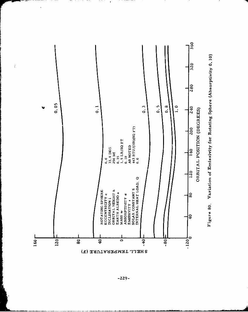
00

ot

aN

44)

En 4

N N

H 0 0

00E--

H 0044-

w 0

u H, 4 ZHc

F4 U< 0

OZý ý> Z 4E- 0 ,P

0 0 0ý 0 0 0 0 0o

-229-

00

4 0

co

14

- I

oo

o %6

4)

.0 0 00

0 0q

•.0..

LA N. 2-3o

(A)4 1. LO) d0 In I H

-230-

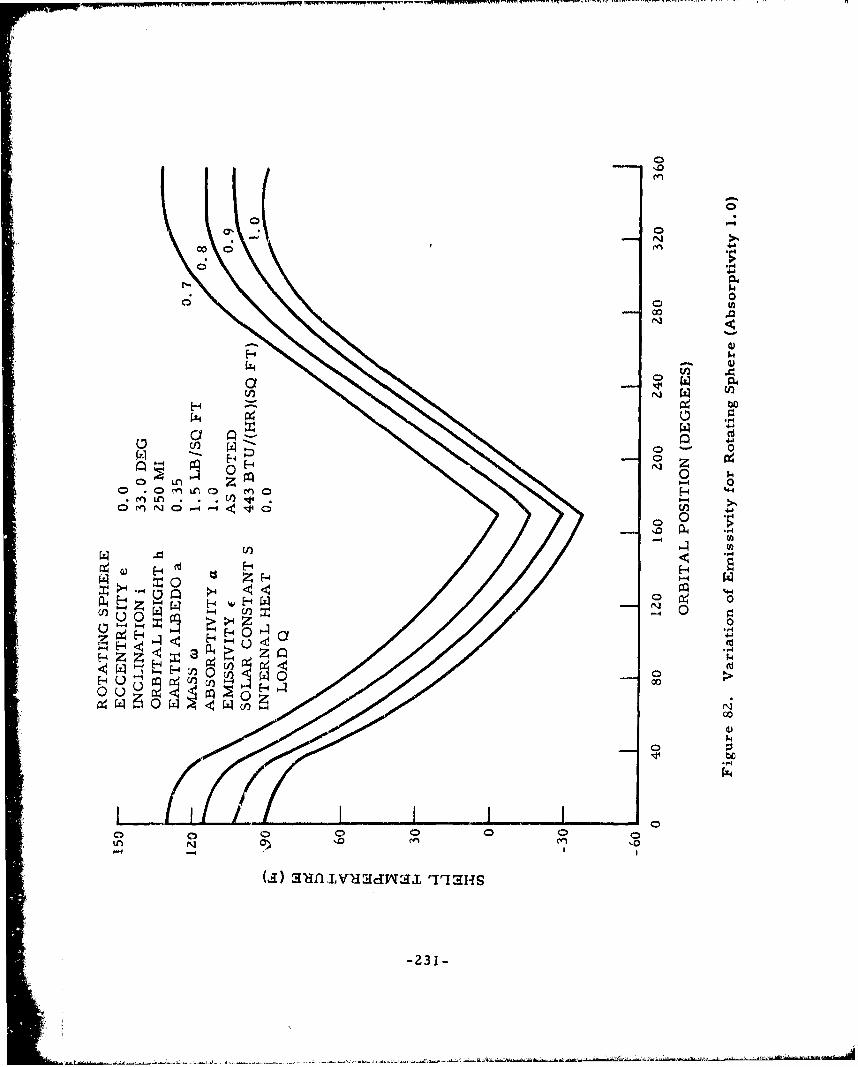
-ra,

00Cl

0* 0°

o 0

N3

F4.a

m• 0

Ile Ln 0

o Lon0 H "

*L -

'O~LO

-14

-_. IF4 --41-

u cn 2-y z

0~~ ch 4

-231-

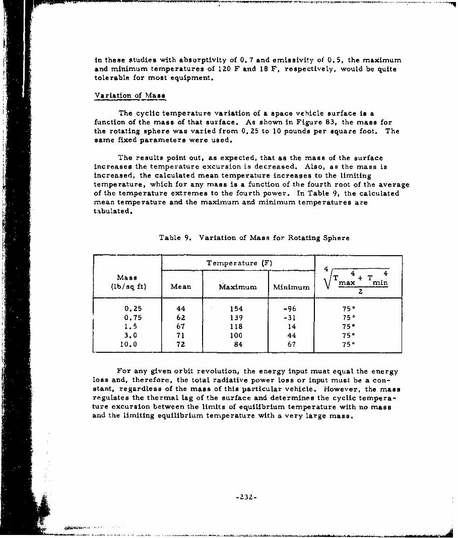
in theme studies with absorptivity of 0. 7 and emissivity of 0. 5, the maximumand minimum temperatures of 120 F and 18 F, respectively, would be quitetolerable for most equipment.

Variation of Mass

The cyclic temperature variation of a space vehicle surface is afunction of the mass of that surface. As shown in Figure 83, the mass forthe rotating sphere was varied from 0. 25 to 10 pounds per square foot. Thesame fixed parameters were used.

The results point out, as expected, that as the mass of the surfaceincreases the temperature excursion is decreased. Also, as the mass isincreased, the calculated mean temperature increases to the limitingtemperature, which for any mass is a function of the fourth root of the averageof the temperature extremes to the fourth power. In Table 9, the calculatedmean temperature and the maximum and minimum temperatures aretabulated.

Table 9. Variation of Mass for Rotating Sphere

* •Temperature (F)Mass -lxTi

(lb/sq ft) Mean Maximum Minimum 2

0.25 44 154 -96 7500.75 62 139 -31 7501.5 67 118 14 7503.0 71 100 44 750

10.0 72 84 67 750

For any given orbit revolution, the energy input must equal the energyloss and, therefore, the total radiative power loss or input must be a con-stant, regardless of the mass of this particular vehicle. However, the massregulates the thermal lag of the surface and determines the cyclic tempera-ture excursion between the limits of equilibrium temperature with no massand the limiting equilibrium temperature with a very large mass.

-232-

* nn*-!

a-

ý4 0

N A0

04

u0 41l

z 0 H 4N

Hu g 1H-4 0~c

19 C4

0O 0

o -o

0

00

o~~C 00

00 NN

C( ) C)Vd3L TIH

-233-

Variation of Internal Heat Load

The cyclic variation in temperature for a rotating sphere is shown inFigure 84 as a function of internal heat load, with the same fixed parametersassumed. The internal heat load was varied from 1.0 to 20 watts per squarefoot. The results indicate, as expected, that the outer shell temperatureincreases as the internal heat load increases. The results at 1.0 watt persquare foot show a maximum temperature of 125 F and a minimum tempera-ture of 22 F. For the case with an internal heat load of 20 watts per squarefoot, the maximum temperature increases to 212 F and the minimumtemperature is 121 F.

Variation of Earth Albedo

In the calculation of the cyclic temperature variation of a satellite inorbit, it is necessary to know the planet's albedo to properly account for theplanet emission and reflected solar energy. As discussed in Section IV on thespace thermal environment, the earth albedo varies because of the planet'ssurface, scattering by clouds and dust in the atmosphere, and molecularscattering by the atmospheric gases.

To determine the effect of various values of the earth's albedo on thecyclic temperature variation, an analysis was made on the rotating sphere.Four values of the earth albedo a were chosen: 0. 2, 0.35, 0.5 and 0.8. Foreach value, various values of the a/c ratio were chosen for each satellite.

The results of the analysis for earth albedos of 0. 2, 0. 5, and 0. 8 areshown in Figures 85 through 87, with the same fixed parameters assumed.

A summary of the results is shown in Table 10, where the maximumand minimum temperatures are tabulated for the various ratios of a/c . Asthe earth albedo is increased, the reflected solar energy from the earth thatis incident on the vehicle is increased; however, the earth's emitted energyincident on the vehicle is decreased because the effective earth temperatureis decreased. The maximum temperature is shown to increase, while theminimum temperature decreases for an increase in albedo. Also, themagnitude of the change increases with increase in a/c ratio.

Variation of Solar Constant

To determine the effect on the cyclic temperature variation of changesin the solar constant, an analysis was made using 433, 443, and 453Btu/(hour)(square foot) as values for the solar constant. For each value,various values of the a/c ratio were chosen for each satellite. The samefixed parameters were used as in the previous runs.

-234-

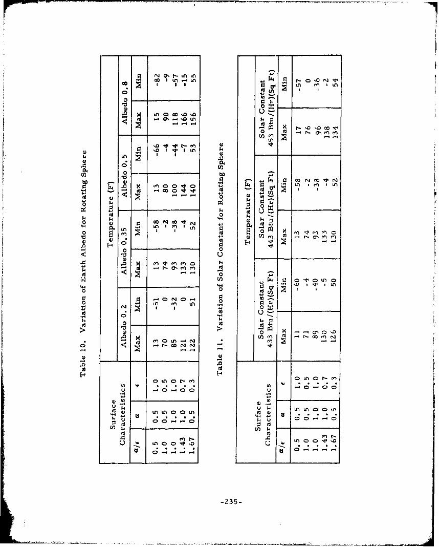
4-1

-4 IL LA 614 :

od 4.

-4- M CI- o 0 Z

14 Ln 1 I

10 C004 0_ _ __ _ _

10 .- ,o~ W - 0N0rz0 Q 41 -41L416 1 41 wco 14

Cd 0

0) 0 4.1 4

.0 (n "___fn o

E- .0 x 404- 0

rn 0

-4. 44$4L

CdD.0 0

-d __ __ __

- .0

.0 CdC

-440 40

-4 3j - .U)

14I- u p 00'44 Co0LH d 40-)4 ts __ _

k d Cd C;C;U0 0 0A0~ u L0 4 '

0n .- 0. 4ý no a ý

-235-

00

Hn 0

oo.%4

H0

0

Hw

aa

H 0-

H0 00a 0A -

.. 4-

ts~ z -

aq >0.U~4 0 4

P4 H> -

L-0 0 00

114

~U) H C)

(d SHlLVH:dH~fL -, 1.44

i-~ -236-

fl 'r ' -- - p m - .. . .. ., . ,. . .. *,

IA;cP4

00

0

tn 04 0-

u 0

-40

0 u C400

LAA

Er

N 0

-0 (0 1 4

r - % P c/ / 0

a4 04-1

00 co 0<0-

-om 00--0

0 0 0 0 0 0 0 0 0 0C

(J) flLHnV-dI3dW~3.L TI'3HS

-23 7-

"' r'0

0 °b

LAf

00

.4 .- 4

->

Vi "i " 0

00

:'i iii 0

0

0II4l

~10 - 4-

0 4

F ° (f) - 4 4-r- 0

0l •0

orl lsjeOl'< o

/- 00

4'00I1-- Itoo

E-4

Nf 00140

1 -238-

1 zH c1" - 0'----

U) 0

0.

.4J

F0 E-N

E44ý

L a -4-4

0

00 00

>0 00Iý

0).,4

%0NIc/c

/29

The results of the analysis for 433 and 453 Btu/(hour)(square foot)are shown in Figures 88 and 89. A summary of the results is shown inTable 11, where the maximum and minimum temperatures are tabulated forthe various ratios of a/c . As expected, the cyclic temperature level isincreased as the value of the solar constant is increased. The magnitude ofthe increase, for the set of conditions assumed for the sphere, appears to beapproximately 0.4 to 0.9 percent in temperature level for a 2. 0 percent

change in solar constant.

COMPARISON OF ROTATING SPHERE AND FLAT PLATE

The cyclic variation in shell temperature for a rotating sphere wascompared with inertially oriented and earth-oriented flat plates, as shownin Figure 90. The following parameters were used for the three surfaces:

Absorptivity a 0.7Emissivity t 0.5Mass oa 1.7 lb/sq ftEarth albedo a 0.35

Solar constant S 443 Btu/(hr)(sq ft)Orbital inclination i 33. 0 degOrbital height h 250 mlInternal heat load Q 0

Also, the back faces of the flat plates were assumed to be perfectly insulated.

The earth-oriented flat plate shows a slight increase in temperature at20 and 170 degrees. This is due to the plate's receiving direct solar energyfor a short time, just after passing the terminator and before going into theearth's shadow, and again when leaving the earth's shadow just beforepassing over the terminator. The temperature level, in general, is higherthan that of the inertially oriented plate because the geometric form factorfor the earth-emitted energy is constant at approximately 0. 88 for the earth-oriented plate. The form factor for the inertially oriented plate varies from0 at 20 degrees to 0. 88 at 185 degrees, where the surface is facing the earthand parallel to the orbit path, and then decreases to 0 again at 335 degrees.

-240-

_- _--

U'l0

.41

C;. 0 044 00

ci4.0 V)

en fE-0

II

/- 4

U) 0

00 -4/N

S-4

000 0 0 0C0000O

-241-

o n N

% 0

0

44 4

41, -4 10..

EA40Ln~ z (

m fl =n 1-4m ~ -n )

~ H~ H. 4 r3U

04 z V)

W4 " (n $4-00 > .0 w

0 *~0 -44

s 0

/ 0 cvý 0/ '-4

N- 00

"(4

a,

OMNO-V1OOO

m~ z

~?zC4)

u '-A4- ( (

z z

000 40

00

NC

000

oo0

0 O0

0 0 0 0 - 040-

CYCLIC TEMPERATURE VARIATION OF EIGHT-SIDED PRISM

A space vehicle configuration, consisting of an eight-sided prism withtwo ends, was considered in order to study the effects of cyclic temperaturevariation of the various sides. The vehicle was assumed to be earth-orientedso that the vehicle axis was on the orbital path. A retrograde orbit of 96.6-degree inclination was used in conjunction with an orbital height of 225 miles.The orientation of the vehicle surfaces in relationship to the earth and sunis shown in Figure 91. The bottom surfaces are 1, 4, and 10, and the topsurfaces are 6, 2, and 8; the sides are 5 and 9, and the ends are 3 forwardand 7 aft. The fixed parameters used for the prism were aa follows:

Absorptivity a 0.7Emissivity £ 0. 5Mass (1 0. 5 lb/sq ftEarth albedo a 0.35Solar constant S 443 Btu/(hr)(sq ft)

The cyclic temperature variation for each surface is shown inFigure 92. To summarize the results and to point out the effects of changingthe surface characteristics and increasing the mass of the individualsurfaces, the maximum and minimum temperatures are tabulated inTable 12. The mass of the surfaces for the second case was 1.5 pounds persquare foot.

Table 12. Maximum and Minimum Temperatures for Eight-Sided Prism

Surface Finish Temperature (F) Surface Finish Temperature (F)

Surface a t Min Max a Min Max

Bottom1 0.7 0.5 160 -17 0.4 0.3 101 374 0.7 0. 5 116 -48 0.8 0. 35 118 23

10 0.7 0.5 116 -48 0.8 0.35 119 25

Top2 0.7 0. 5 315 -249 0.1 0. 1 106 476 0.7 0.5 253 -227 0.1 0.075 96 528 0.7 0. 5 258 -226 0.1 0. 075 101 57

Sides5 0.7 0. 5 8 -123 0.8 0. 15 99 519 0.7 0.5 22 -123 0.8 0. 20 89 34

Ends3 0.7 0. 5 323 -123 0.1 0. 1 89 397 0.7 0.5 323 -122 0. 1 0. 1 101 47

-244-

3--

78 6

97

LINE FROM CENTEZ R OF EARTH10 •TO CENTER OF VEHICLE

ORBIT PATH

CENTER OF EARTF

S96. 60

A20 DCELESTIAL EQUATORASC ENDINGNODE

SUNDIRECTION

Figure 91. Diagram of Earth-Oriented Eight-Sided Prism

-245-

WA0

crNN

f4

44.4 0

c~00N

* ~0Ole

0C)IAV

-'160

* 0

En-,.4

Q.4

W C4

"P4

M E-44

O n 0 f r n r- IL 0

CD CN .1 06

0 0

;q

ZH 0

oU 0 Z >'

0 0 ~

z z [-4.C4

u

-4)

CDC)ccý C0 CD 0

-247-4

The effect of mass in reducing the temperature spread betweenmaximum and minimum temperatures is shown by surface 1 (the bottomsurface which always faces the earth) when compared with the earth-orientedflat plate in Figure 90. For the case with extremely small surface mass,surface 1 reaches the shadow side equilibrium temperature of -17 F. Whenthe mass is increased to 1. 5 pounds per square foot and absorptivity andemissivity are changed to 0.4 and 0.3, respectively, the maximum andminimum temperatures are 101 and 37 F. With the proper choice of surfacefinish and a reasonable structural mass, these particular vehicle surfacescan be maintained within reasonable temperature limits.

DISCUSSION OF ASSUMPTIONS

1. It is assumed in this analysis that the earth can be represented gravita-tionally by the zero-order and second-order spherical harmonics of itspotential. The presence of harmonics in the earth's gravitational potentialcauses periodic and secular variations in several of the orbital elements.Only the secular perturbations which result in regression of the nodesand advance of the perigee position are considered in the analysis. Otherperiodic changes have negligible effect upon the shadow intersectionproblem.

2. A rigorous specification of the position at which the satellite enters andexits the earth's true shadow leads to needlessly complicated expressions.For this reason the following simrplifications concerning shadow geometryare assumed:

a. The earth is spherical with its radius equal to 3960 statute miles.b. The earth's shadow is cylindrical and umbral (sun at infinity).c. Penumbral effects are ignored.

The error involved is extremely small even when large orbits are con-sidered. For instance, a satellite in a circular orbit with an altitude of10,000 miles has an orbit period of approximately 560 minutes, withperhaps 50 minutes spent in earth shadow (depending on orbit orientation).By assuming a cylindrical earth. shadow and ignoring penumbral effects,the analysis uses an umbral shadow time that is about 50 seconds longerthan the true umbral shadow time. This is a negligible error. For a1000-mile-altitude circular orbit, the negligible error is approximately18 seconds in an orbit period of 118 minutes. Additionally, it should bementioned that the assumption of no penumbral effects tends to lessen theabove errors introduced by the assumption of cylindrical umbral shadow,so that there is almost zero error from a thermal analysis standpoint.

3. It is assumed that all thermal radiation considered in the analysis,except solar radiation, is in diffuse form. Fortunately most thermalradiation is in diffuse form, which is relatively simple to analyze whencompared with specular radiation.

-248-

4. It is assumed that direct sola, radiation impinges upon the earth and

upon the satellite with parallel rays, due to the great distance between

the sun and its planets. Almost zero error is introduced into the analysis

by the assumption.

5. In all cases, it is assumed that the earth emits as a black body andis in a state of thermal equilibrium (i. e. , the planetary emittedenergy is equal to the absorbed solar energy). It is also assumedthat the earth emission is a constant at any point on its surfaceand does not vary from day to night. These are reasonableassumptions because little is known of the actual spectral andlocal variations in the planetary emitted radiation.

6. The earth reflected solar radiation is assumed to follow the cosinelaw (i. e. , it is a maximum at the subsolar point and decreases tozero at the terminator). This assumption greatly simplifies theanalysis and is quite accurate except in the region of theterminator, where a slight error is introduced.

=r

7. In all cases, the planetary albedo is assumed to be constant overthe surface of the planet, and the planet is assumed to be a diffusereflector. This is done because of the complications of theproblem and because local variations are almost impossible to

Lm define.

8. In all cases, conduction and convection between the satellite andits surroundings are neglected. This is reasonable because orbitalheights are usually too far above the atmosphere for these types ofthermal effects to appear.

9. It is assumed that the absorptivity of the vehicle surface toplanetary thermal emission is equal to the emissivity of the vehiclesurface. Since the effective temperature of the earth and thetemperatures of most vehicle surfaces are nearly the same, thisassumption is validated by Kirchhoff's law.

10. Any scattering effects of direct solar radiation upon the satellitedue to the earth's atmosphere are ignored. It is felt that this willintroduce a negligible error into the analysis.

11. The geometrical configuration factor from the spherical satelliteto earth was calculated with the assumption that the satellite is apoint source in space. The assumption is valid if the satellite isuniform in temperature, which it would be if spinning or if its shellhad a very high thermal conductivity.

"-249-kI

Section IX

CONCLUSIONS

ANALYSIS TECHNIQUES

This report has reviewed the basic principles of therral radiation andhas presented several available methods of radiation heat tranafer analysis,with emphasis upon the situation encountered by a vehicle in space,

An IBM 7090 program has bean written (Section V) with which it ispossible to obtain space irehicle shell temperaturee and the incident radiantenergy impinging upon the vehicle fhom its space environment. Thesignificance of this prograin is that it will accurately simulate any ellipticalor circular orbit into which a satellite may be placed.

In the field of general radiation heat transfer analysis, a comparisonhas been made between various methods of analysis in which the accuracyand versatility of the radiosity analog network method is pointed out. It ishoped that a more widespread use of this relatively new technique will occur

in industry.

One of the lnost difficult areas in the analysis of radiation heat transferis the proper calculation of the geometric configuration factor. Aconsiderable amount of tabulated data is presented in this report (Section VII ),some of which has been heretofore unpubliahed. lj conjunction with thisreport, an IBM 7090 program (Reference V7) has been written wVhich willcalculate the configuration factor bezween two plane areas in anyorientation with respect to each other. While presently limited in scope,this program has promise of being developed into an extremely valuabletool for the heat transfer engineer.

PROBLEM AREAS

Thermal Analysis of Nondiffuse Radiation

A problem area which came to light in the preparation of this reportand which needs further investigation concerns the thermal analysis ofnondiffuse radiation. Presently used methods of analysis make the basicassumption that all radiant energy is diffuse, whereas, in actuality, radiantenergy usually exists in partly diffuse, partly specular form. Datapertaining to directional emissive properties are very limited, almost not

-25 1-

BSLANKPG

available. Fortunately, the majority of radiant energy does exist inessentially diffuse form, so that presently available analytical methods areusually applicable. There are many occasions, however, when this is nottrue, and the engineer is forced to make questionable approximations.

Calculation of Geometric Configuration Factors

Another problem area concerns the calculation of geometricconfiguration factors, an essential part of radiation heat transfer analysis.This is probably the most tedious and time consuming job encountered in theanalysis. Although much work has been done in this area, data are stilllimited. For other than simple shapes, numerical or mechanicalintegrators must be utilized, and this is a time consuming process. Asnie-.tioned, there ia hope that an IBM program can be developed to aid inthis arca.

Measurement and Presentation of Data

The accurate thermal analysis of space vehicles depends heavily on theavailability of accurate data on the thermal properties of materials,including solids, liquids, and gases. These properties include absorptivity,emissivity, conductivity, and specific heat, and they should be known for theentire temperature range of interest and as a function of wave length, angle,and pressure, as applicable. Much of the published data on thermalproperties, however, are sub ject to serious question; handbook-type datagenerally represent only average values over a narrow range of conditions.The common practice of not differentiating between normal and hemisphericalemissivity can lead to serious errors in temperature prediction.

The lack of accurate information on thermal properties jeopardizes theaccuracy of thermal analyses and probably will lead to in-flight failures.With the mult.plicity of data collecting and publishing agencies, theinconsistencies and contradictions between published data on the samematerials creates increasing confusion. So it is concluded that standardizedmethods of measuring and presenting data on the thermal properties ofmaterials are needed.

Effects of Space Environment on Space Vehicles

It is generally accepted that space vehicles will be subjected todeteriorating influences in a space environment. In some cases, theragnitude of these external influences is known. In almost every case,however, the effect of these influences on space vehicle materials is eitherincomplettly known or totally unknown. The data from actual satellites arevery meager and are being accumulated too slowly to support current needs.

-252-

Although the accumulation of data relative to the effects in materials of someof the components of the space environment is progressing on many fronts,the present lack of data casts doubt on the current designs of space vehicles.One factor that seems to be receiving little experimental attention is theeffect of micrometeorite erosion on the absorptivity and emissivity ofsurface coatings. The short-term effects may reasonably be neglected; butfor long durations, the deterioration may become quite pronounced.Comparative data on absorptivity and emissivity before and after amultiplicity of simulated micrometeorite impacts on representative coatingsare needed as a guide for future vehicle designs.

The lack of accurate and complete information on the effects of thespace environment on the absorptivity and emissivity of surface coatingsmakes the design of passive temperature control systems very questionablefor long-duration vehicles. To compensate for unknown variations, it maybe necessary to resort to semipassive or active temperature controlsystems.

The effect of the low-pressure environment encountered in space isknown to cause a significant increase in thermal resistance acrossstructural joints, whether they be bolted, riveted, or spot-welded. Thisthermal resistance is almost impossible to predict accurately, and it mustbe eliminated in conduction cooling paths and other thermally significantstructures. At the present time, there is available a vacuum-resistantsilicone type grease, often called "space grease, " which seems to offergreat promise in reducing contact resistance when applied to a structuraljoint. There are other materials, such as aluminum foil, that might alsoprove to be effective upon investigation. Although some work has been donein this area, further effort is needed.

I' --•"

III

Section XANNOTATED BIBLIOGRAPHY

This annotated bibliography was prepared as a result of a literaturesurvey conducted by the reference staff of the Technical Information Centerof S&ID.

PERIODICALS

Advances in Astronautical Sciences

Vol 3, 1958, p 22-1 - 22-11.Temperature equilibrea in space vehicles. R. Cornog.

The equilibrium temperature reached within a space vehiclemoving within the solar system is discussed. The effects ofvehicle configuration, vehicle attitude, surface properties, andinternal heat release are evaluated. Particular attention isgiven to methods of vehicle design whereby the range of equilib-rium temperatures can be set at some desired value.

Aero/Space Engineering

Vol 19, March 1960, p 58-60, 64.Evaluation of thermal problems at relatively low orbital altitudes.L. D. Wing.

Presented here is a simple way to estimate the maximum andminimum heat inputs experienced anywhere on the outer skinface of an orbiting vehicle.

i,i

Vol 19, October 1960, p 16- 19, 56, 58, 59, 62.Surface effects on materials in near space. F. J. Clauss.

The problems associated with the behavior of materials in space,including passive temperature control are discussed.

-25 5-

movng ithn te ola sytemis isussd, he ffets o u.A

Aero/Space Sciences, Journal of the

Vol 26, December 1959, p 772-774.Space vehicle environment, thermal radiation. C. Gazley and others.

"The primary mode of heat exchange between, a space vehicle andits environment is radiation. " A brief summary is presented ofpresent knowledge of such heat exchange, as it depends on solarrationation, neighborhood of a planet, and space vehicle itself.

Vol 27, February 1960, p 146-147.The minimum-weight straight fin of triangular profile radiating tospace. E. N. Nilson and R. Curry.

A basic property of the nonlinear differential equation expressingthe radiation of waste heat from a spacecraft yields a method ofsolution which is an extension of the solution of the problem ofdetermining the triangular fin of optimum shape for dischargingsuch heat by convection.

American Physical Society, Bulletin of the

Vol 3, 1958, p 303.Temperature control problems of artificial satellites. G. B. Heller.

American Rocket Society, Journal of the

Vol 17, 1957, p 34-35.Some remarks on the temperature problem in the interplanetary rocket.R. L. Sternberg.

Annals of the IGY (Vol 6, Manual on Rockets and Satellites)

Vol 4, 1958, p 304-310.The IGY earth satellite program: satellite-temperature control (summaryof paper by L. Drummeter and M. Schoch presented at IGY Rocket-SatelliteConference, Washington, D. C. , 30 September - 5 October 1957.

ARS Journal

Vol 29, May 1959, p 358-361.Thermostatic temperature control of satellites and space vehicres.R.A. Hanel.

The temperature of satellites and space vehicles varies consid-erably with orbital conditions. To achieve greater reliability and

-256-

efficiency in long-life instruments, an automatic temperaturecontrol is highly desirable; a radiation thermostat performingthis function is discussed. The suggested method regulates

temperature by adjusting the effective absorptivity and emis-sivity. Bimetallic strips automatically move a light shield

which exposes surfaces with high and low absorptivity-to-emissivity ratios. No internal power source is needed.Calculations demonstrate the effectiveness of the radiationthermostat. The temperature of the satellite's instrumentscan be kept constant within a few degrees of the design value,

regardless of orbital conditions, internally dissipated power,and some erosion of skin coatings.

Vol 30, April 1960, p 344-352.Thermal control of the Explorer satellites. G. Heller.

Thermal control of the Explorer satellites is discussed. Thetheoretical studies that were made prior to the launching of thesesatellites are described, and examples of relationships are pre-sented in graphs. The lower limit of the instrument temperaturewas 0 C (determined by the efficiency of the chemical batteries).

The upper limit was specified as 65 C (based on long-timetemperature limits of transistors in the electronic package).This paper relates some of the studies, describes the measuringresults of telemetered temperatures, and evaluates expected andobtained data.

Vol 30, May 1960, p 479-484.Solar heating of a rotating cylindrical space vehicle. A. Charnes and

S. Raynor.

Solar heating in a space vehicle idealized as a thin-walled circularcylinder rotating with uniform velocity about its geometric axis isstudied for a situation in which heat transfer by convection and

heat exchange within the cylinder is negligible. The nonlinearproblem is approximated through a perturbation analysis, anddetailed estimates are made of the parameters of interest forvarious ranges of speed of rotation. An estimate of the error

between the exact and perturbational approach is made in the

case of an illustrative example which might be expected to entailan extreme deviation.

-257-

Astronautical Sciences, Journal of the

Vol 5, Autumn-Winter 1958, p 64.Temperature equilibrea in space vehicles. R. A. Cornog.

The equilibrium temperature reached within a space vehiclemoving within the solar system is discussed. The effects ofvehicle configuration, vehicle attitude, surface properties andinternal heat release are eva.iatad. Particular attention isgiven to methods of vehicle design whereby the range of equi-librium temperatures can be set at some desired value.

Astronautic s

Vol 5, April 1960, p 40-41, 105-106.Thermal protection of space vehicles. P. E. Glaser.

The near-steady heating conditions encountered in long-termspace flight have sparked development of integrated systemsdesigned to protect the vehicle while combining maximuminsulating effectiveness and low weight.

Astronautics, Journal of

Vol 3, Spring 1956, p 4-8, 26.

Thermal control in a space vehicle. P. E. Sandroff and J. S. Prigge.

Astrophysical Journal

Vol 131, January 1960, p 68-74.Use of the equation of hydrostatic equilibrium in determining the tempera-ture distribution in the outer solar atmosphere. S. R. Pottasch.

The purpose of this paper is to use the observed variation ofelectron density between 3000 kilometers and 20 solar radii and,assuming hydrostatic equilibrium, to derive a distribution ofelectron temperature in this region. The plausibility of thetemperatures derived in this way is discussed.

Vol 131, March 1960, p 459-469.

Radiometric observations of Mars. W. Sinton and J. Strong.

Aviation Age

Vol 30, August 1958, p 174-180.

How to find thermal equilibrium in space. R. E. Hess and A. E. Weller.

-- 58-

IRE Transactions on Military Electronics

Vol Mil-4, April-July 1960, p 98-112.Problems concerning the thermal design of Explorer satellites.G.B. Heller.

The thermal design of the Explorer VII satellite in described. Athermal testing program conducted in the vacuum chamber with aprototype of Explorer VII is described, and some preliminaryresults of temperature m-easurements of the Explo;'er VII aregiven.

Iron Age

Vol 182, 6 November 1958, p 105-107.Ho-a metals help control satellite's temperature. P. M. Unterweiser.

Case histories are considered concerning two small Navysatellites. The problem of controlling the temperature of thesatellite's magnesium shell, which was subjected to periodicvariations, was solved by gold plating its surface and coveringit with an evaporated layer of silicon monoxide. This coatingwas then overlaid with opaque film of evaporated aluminum forhigh reflectivity.

Izvestiya Akademii Nauk SSSR, Seriya Geofizicheskaya

Vol 4, April 1957, p 527-533.Termperature regine of an artificial earth satelli•.e. A. G. Karpenko andM.I. Lidov.

Jet Propulsion

Vol 27, October 1957, p 1079-1083.Skin temperatures of a satellite. C. M. Schmnidt and A. J. Hanawalt.

The need for a workable artificial earth satellite has beenestablished both icr reconnaissance and as a prerequisite forspace travel. A.a attendant problem in the design of such t

vehicle is the control, and therefore the prediction, of tempera-tures that will exist in flight. Previous papers on this topic havebrought out many salient features of such predictions, but havenot been entirely realistic. The present. paper attempts toimprove on these assumptionA and gives numerical computationsfor a particular configuration considered feasible for a satellitedesign. The example investigated is a nonrotating cylindrical

-259-Ii'

shell with one end point earthward. The problem of anrDl;,sxis largely one of geometry, involving spacewise as well amtimewise variations in skin temperature. The skiz. tempera-

tures that will exist are very dependent on the properties oftha surface, particularly emissivity and absorptivity, largevalues producing the widest range in surface temperatures.

By proper choice of these parameters, this range can begreatly controlled. In particular, the mean temperature ofthe satellite skin is primarily a function of ol/e. For thespecific configuration considered herein, nominal limits on theskin temperatures are -200 and +400 F.

Optical Society of America, Journal of the

Vol 47, 1957, p 261-267.Optical problems of the satellite. R. Tousey.

Vol 49, September 1959, p 918-924.Temperature stabilization of highly reflecting spherical satellites.G. Hass, L. F. Drummeter, Jr., and M. Schoch.

Report of NRL Progress

May 1958, p 1-7.Satellite temperature control. L. F. Drummeter, Jr. , and M. Schoch.

Science

Vol 127, 11 April 1958, p 811-812.Temperatures of a close earth satellite due to solar and terrestrialheating.

See Aero/Space Engineering, Vol 17, No. 10, October 1958, p 104.

SAE Journal

January 1959, p 54-55.Water and ammonia evaporators show promise in cooling orbital space

vehicles. J. S. Tupper.

See Aero/Space Engineering, Vol 18, No. 5, May 1959, p 102.

-260-

Vistas in Astronautics

VWl I. p 157-158.The temperature equilibrium of a space vehicle. J. E. Navgle.

The equilibrium temperature of a space vehicle is considered. Inspace, away from the earth, the vehicle will come into radiativeequilibrium with the sun's radiation. The skin temperature of thevehicle will rise until the amount of energy radiated by the vehicleis equal to the sum of the energy absorbed from the sun and thatproduced in the vehicle itself. The absorbed solar energy is in thevisible portion oi the spectrum, whereas the emitted energy ie inthe far infrared. Equilibrium temperatures attainable with existingmaterials are too high; the basic problem is one of keeping thevehicle cool. The problem of interest ia the effect of th6 envi-ronment on '-he surface of such vehicle. Additional research isneeded both aa to ..he nature of the environment to be encounteredand as to the effect of this environment on the surface.

Western Machinery and Steel World

Vol 50, October 1959, p 72-74.Coatings for space vehicles. J. L. Snell.

At Jet Propulsion Laboratory, California Institute of Technology,ordinary types 430 and 410 stainless steels, used to encasedelicate instrument capsules, were made to have thermalcharacteristics not yet pos3ible in metal alone. Discussed aru thetechniques for temperature control, fabrication of the final assembly,and application of special process coatings of Rokide A by CooperDevelopment Corporation, Monrovia.

REPORTS AND PAPERS

Air Force Cambridge Research Center

TN-58-633, March 1959.The temperature of an object above the earth's atmosphere. M. H. Seavey.(AD-208, 863)

The equilibrium temperature of an object above the earth's atmos-phere is calculated by considering the thermal radiation balancefor the object.

-z61-

American Rocket Society

Preprint 383-56, 1956.Skin temperatures of a satellite. C. M. Schmnidt and J. S. Prigge.

Army Ballistic Missile Agency

DV- TN-73-58, 1958.Thermal problems of satellites. G. Heller.

California Institute of Technology

EP-481Satellite temperature measurements for 1958 Alpha - Explorer I.

External Publication 514, Z June 1958.Scientific results from the Explorer satellites. A. R. Hibbs.

A brief history of Explorer satellite launchings is given, togetherwith a description of payload instrumentation. Results of experi-ments made in the areas of tempe. itures of both case and internalinstrumentation, micrometeorite activity, and cosmic rayintensity are summarized. The results of preliminary analysesof these various measurements as carried out by the responsibleinstitutions are presented, and their implications for futuremeasurements of this type are discussed.

External Publication 647, 7 May 1959.Temnperature control in the Explorer satellites and Pioneer spaceprobes. L. P. Bulvalda and others.

The Jet Propulsion Laboratory participated in ve Explorer andJuno II programs in the areas of payload design and method ofachieving temperature control. This publication describes thebasic theory for the passive temperature control of satellites andspace probes and the application of this process to the Explorerand Pioneer III and IV vehicles. Some results of in-flighttemperature meacurements are also presented.

Memo 20-194, 15 February 1960.Radiative properties of surfaces considered for use on the Explorersatellites and Pioneer space probes.

Spectral reflectance data in graphical forrn and tabular abporptance-emittance data are presented for surface materials consideredfor use on the Explorer satellites and Pioneer space probes. Thesurfaces ranged from bare aluminum, titanium, and stainless

-262-

..f..f.....

steel to painted coatings, coatings of Rokide A, and anodized andplated coatings. A brief review of the temperature controlproblem is presented as background information.

Progress Report 20-294, 28 March 1956.The temperature of an orbiting missile. A. R. Hibbs.

The successful operation of radio equipment carried in an orbitingmissile requires fairly close control over the temperatures towhich the equipment is subjected. This temperature is controlledby two factors. First, the temperature of the outer shell of themissile depends on radioactive transfer between the missile andits invironment (sun, earth, and empty space). Secondly, thetemperature of the equipment inside the missile depends on heattransfer from the shell (directly by radiation and through thestructure by conduction). The analysis presented shows how the

average temperature of the outer shell can be controlled (for agiven missile shape, orientation, and trajectory) by a correctchoice of surface coatings. It also indicates that the limits oftemperature variation of the enclosed equipment can be held towithin a few degrees of this average shell temperature byadequate insulation. Numerical calculations indicate the neces-sary characteristics of the coating and insulating materials.

Progress Report 20-319, 11 April 1957.Evaluation of the absorptivities of surface materials to solar andterrestrial radiation, with plots of the reflectances (at wave-lengths of0. 4 to 25 m) for 10 sample materials including 2 types of fibrous-glassreinforced plastic. W. S. Shipley.

Progress Report 20-359, 3 September 1958.Contributions of the Explorer to space technology. J. E. Froehlich andA.R. Hibbs.

The philosophy of the Explorer programs is presented and demon-strated in the description of missile design and flight operation ofthe Explorer vehicles. Scientific measurements of cosmic rayintensity, temperature environment, and micrometeorite densitiesare described, and the significance of these measurements isdiscussed.

-263-

General Electric Company, Aerosciences Laboratory

T. I. S. Report R60SD386, August 1960.A method for calculating the thermal irradiance upon a space vehicle anddetermining its temperature. T. L. Altshuler.

A method is presented for determining the thermal irradianceupon a space vehicle as a result of direct radiation, planetarythermal radiation, and planetary albedo. From this information,the temperature of a space vehicle can be obtained. Calculationscan be made for various space vehicle altitudes above a planetand for various solar angles with respect to both the planet andspace vehicle. The planets and natural satellites considered arethe earth, moon, Mars, and Venus.

Grumman Aircraft Engineering Corporation

Report XplZ. ZO, May 1960.Determination of thermal radiation incident upon the surfaces of an earthsatellite in an elliptical orbit.

A procedure is presented for determining the radiation incidentupon a satellite in an elliptical orbit. The satellite is treated asa set of plane areas, each area identified by the direction cosinesof its outward normal with respect to a satellite coordinate system.This system is based on orbit orientation. Radiation emitted byand reflected by the parent body is computed by integrating overthe spherical cap seen by the satellite. Solar radiation is consid-ered constant. The method is applied to a hypothetical satellitein orbit. Comparisons of incident radiation have been madebetween rotating and nonrotating satellites in the same orbit.This type of comparison might be used to decide whether or notsatellite rotation is desirable, and if so, to what extent. It isalso possible to compare different orbits for the same satelliteto optimize radiation to its surface.

IGY Satellite Report Series No. 3

Paper No. 4, 1 May 1958.Satellite temperature measurements for 1958 Alpha - Explorer I.E. P. Buwalda and A. R. Hibbs.

-z64-

Internation Astronautical Federation

September 1956.Studies of a minimum orbital unmanned satellite of the earth: part III.Radiation and equilibrium temperature, D. T. Goldman and S. F. Singer(Astronautica 0/86-733, Zeilen Garmond, Presented at 7th Congress ofIAF).

National Academy of Sciences, National Research CounciA Mate-ialsAdvisory Board

MAB-155-M, 20 October 1959.Materials problems associated with the thermal control of space vehicles.

National Aeronautics and Space Administration

TND-357, June 1960.Determination of the internal temperature in satellite 1959 Alpha(Vanguard II). V. R. Simar and others.

Satellite 1959 Alpha was equipped so that accurate measurement

of the mini-track beacon frequency (with the doppler componentremoved) was sufficient to determine the satellite's internaltemperature. To provide a precise measurement of this fre-quency, a sensitive receiving system, utilizing a highly stablebut tunable first local oscillator and a noise-eliminatingtracking filter, was developed. In addition to the temperaturedetermination, other information such as roll rate and rocket

'*_performance was obtained from the observations.

North American Aviation, Los Angeles Division

NA-54-586, 2 July 1954.A proposed research and development program directed toward reliabletemperature prediction of aircraft structural components: part IV.radiation effects. M. R. Kinsler.

NA-56-68, 12 April 1957.Performance specifications for a versatile spectrophotometer for thermalradiation measurements. E. L. Goodenow and M. W. Peterson.

NA-56-69, 12 April 1957.Possible designs for a versatile spectrophotometei for thermal radiationmeasurements. E. L. Goodenow and M. W. Peterson.

NA-57-41, 12 April 1957.Spectrophotometer for thermal radiation studies. P. E. Ohlsen andG.A. Ethemad.

-265-

, . .

NA-57-707, 28 June 1957.Control of external akin temperatures by use of selective finishes.F G. C. Frey.

NA-57-330, 23 July 1957.Spectral and total radiation data of various aircraft materials.P. E. Ohlsen and 0. A. Etemad.

NA-57-707-l, 5 Fuiaruary 1958.Emissivity aad ruflectance of selected surface coatings. R. E. Klemm.

NA-58-525, March 1956. (Secret)Thermo considerationa for the design of satelloid vehicles.

NA-58-1599, 5 December 1958. (Secret)Preliminary thermo analysis of extensive surfaces protection systemrequiremente for B-70 air vehicle. P. Ohlsen and A. Nusenow.

NA-5Q-102, 11 August 1959. (Secret),7reliminary thermodynamic analysis of I. R. seekers for B-70.

NA-59-53, 1959. (Secret)Thermal radiation characteristics of B-70 weapon system.X. Klemm and others.

NA-59-53-1, 31 July !959. (Secret)Thermal radiation characteristics of B-70 weapon system.R. Klemm and others.

NA-59-1887. (Secret)

B-70 infra-red radiation and radar X-section. W. Kemp.

Offi-e of Naval Research

IRIS Proceedings (Confidential), Vol 4, No. 1, 1959, p 115-27.Temperature stabilization of Vanguard satellites, theory and practice.L. F. Drummetei and G. H. Hass. (Chapter referenced is unclassified)

The temperature of an orbiting satellite depends on radiationbalancing and on the parameters which control the radiationenvironment. The latter include orbital characteristics andthe surface properties of the satellite skin. The surfaceproperties are absorptance for extraterrestrial sunlight andhemispheric emittance, aiLd the governing parameter is the ratioof these. Adjustment of the surface parameters permits apassive system of temperature stabilization and is used in theVanguard program. For visibility reasons, the Vanguard

-266-

devices had to ha'ie specular reflecting surfaces with highvisible reflectiimn. For satisfactory temperatures, the infraredproperties had to be modified to increase the surface emittance.

Tho solution consisted of overcoating polishad metal with avacuum coating of partially oxidizad SiO. This material istransparent in the visible but has infrared absorption between8 and 12 n'icrons. A film 0. 54 micron thick has an emittanceof 0. 13 at 20 C; the ernittance increases to 0. 40 for a film 1.2microns thick. Satellite coating is done in a 7Z-inch evaporatorin a special rotating jig designed to provide relatively uniform

thickness.

Oklahoma State University, Engineering Experiment Station

Publication 112, April 1960.Radiation heat transfer and thermal control of spacecraft. F. Kreith.

The material in this report was presented as a lecture series.The basic principles of radiation are reviewed. The mostimportant aspects of thermal control and solar power generationfor spacecraits and satellites are covered, as are methods fordetermining radiation properties with special emphasis onselective surfaces. Radiation processes in an enclosure (suchas a cavity receiver of a solar powerplant or the interior of aspace platform), important energy sources in the solar system(sun and planets), and the atmosphere of the earth are discussed.

The fundamentals of solar powerplant design for spacecraft aregiven.

University of Wisconsin

1960.The thermal radiation balance experiment on board Explorer VII.V. E. Suomi.

The radiation energy budget of the earth is determined by themagnitude of three radiation currents: (1) the direct radiationfrom the sun, (2) the fraction of this that is diffusely reflectedby the earth, the clouds, and the atmosphere, and (3) thefraction that is converted into heat and is ultimately reradiatedback to space in the far infrared portion of the spectrum. OnExplorer VII, three radiation currents are measured with simplebolometers in the form of hollow silver hemispheres. Thehemispheres are thermally isolated from, but in close proximityto, specially aluminized mirrors. The image of the hemisphere,which appears in the rmirror, makes the sensor look like a fullsphere. Two of the hemispheres have a black coating whichmakes them respond about equally to solar and terrestrial

-267-

radiation. Another hemisphere, coated white, is more sensitiveto terrestrial radiation than to solar radiation. A fourth has agold metal surface which makes it more sensitive to solar thanto terrestrial radiation. The information telemetered to theearth's surface is the sensor temperatures. The radiationcurrents are obtained by using these temperatures in heat-,balance equations. Sample calculations are given and resultsare described.

Wright Aeronautical Development Division

WADD TR 54-42, 1954.Total normal emissivities and solar absorptivities of materials.G.B. Wilkes.

BOOKS

Clauss, F.J., Editor

Surface effects on spacecraft materials. Wiley, 1960, p 3-54.Effect of ourface thermal-radiation characteristics on thetemperature -control problem in satellites. W. G. Gamack andD.K. EdvwLrds.

The &atellite thermal problem is reviewed. Satellite tempera-tures are shown to depend upon exterior thermal radiationcharacteristics, external environment, orbit geometry, andinternal power generation. A method is presented for estimating"uncertainties in the predicted temperatures brought about byuncertainfies in the determining variables. Graphs and formulasnecessary for application of the method are included inappendixes. A survey is made of the origins of uncertaintiesin the deternLining variables. Uncertainties in radiation charac-teristics of surfaces are shown to arise from lack of precisiQnin measurements, lack of control in manufacturing processes,anid lack of surface finish stability. Numerical examples clearlyillustrate the importance of the uncertainties in radiation charac-teristics. Methods of reducing uncertainties in internal satellitetemperatures through careful selection of surface finishes aregiven, and active control systems are discussed,

Surface effects on spacecraft materials. Wiley, 1960. p 55-91.Temperature control of the Explorers and Pioneers. T.O. Thostenand others.

The Jet Propulsion Laboratory participated in the launching ofthe Explorer satellites and the Juno II space probes (Pioneers IIIand IV), This participation included payload design and themethod of achieving temperature control. This paper describesthe basic theory for the passive temperature control of satellites

-268-

and space probes and the application of this process to theExplorer and Pioneer III and IV vehicles. Some results of in-flight temperature measurements are also presented.

Surface effects on spacecraft materials. Wiley, 1960, p 92-116.

Coatings for space vehicles. J. C. Raymond.

Six general types of coatings and some of their properties ofinterest for spacecraft applications are discussed: organiccoatings, electrodeposited coatings, phosphate-bonded ceramiccoatings, porcelain enargels, high-temperature frit-refractoryceramic coatings, and flame-sprayed ceramic coatings. Thefour types of ceramic coatings are discussed in detail. A briefdescription of metal preparation, application and firing of coat-ings, and coating properties is included. Values for totalhemispherical and normal spectral emittance are given where

available.

Surface effects on spacecraft materials. Wiley, 1960, p 152-63.

Vanguard emittance studies at NRL. L. F. Drummeter, Jr., andE. Goldstein.

The general problem of passive control of temperature in theVanguard devices involved many problem areas. This paperpresents procedures and results associated with one phase of the

thermal work-.the studies of emittance. The total hemisphericemittances of several materials were measured by coating themon sample bodies, suspending the bodies in an evacuated chamber,and heating them. The emittances of A1203 and SiO coated onaluminum, gold, and silver surfaces, of polished tungstencarbide, and of silicon solar cells were measured.

Surface effects on spacecraft materials. Wiley, 1960, p 182-94.Some methods used at the National Bureau of Standards for measuringthermal emnittance at high temperatures. J. C. Richmond.

At the National Bureau of Standards, the Radiometry Section ofthe Atomic and Radiation Physics Division and the EnameledMetals Section of the Mineral Products Division are concernedwith thermal emittance measurements. The investigations of the

Radioetry Section include absorption of radiation and the inter-pretation of absorption spectra (including infrared absorptionspectra), accurate evaluation of materials for use in wavelength

calibration of spectrometers, and calibration of standards ofspectral radiation and standards for total radiant energy. TheEnameled Metals Section is engaged in developing instrumentationand procedures for determining total hemispherical emittance,

-- 69-

normal spectral emittance, and spectral reflectance of a widevariety of materials, including ceramics and ceramic-coated

metal.

Hynek, J. A., Editor

Astrophysics, a topical symposium. 1951, p 259-301.The sun and stellar radiation (chapter 6).

Radiation and stars from the sun are discussed, including thespectral energy curve of the sun and the solar constant. Thevarious sources of heat in the photosphere are described.These include radiation from stars and planets, radiation fromvariable stars, and planetary heat. Radiation properties of themoon are also taken up.

Kuiper, G. P. , Editor

The solar system: vol 2. The earth as a planet. University of ChicagoPress, 1954, p 726-738.Albedo, color and polarization of the earth. A. Dajon.

Malone, T. F., Editor

Compendium of meteorology. American Meteorological Society, 1951,p 25-28.Solar radiant energy, its modification by the earth and its atmosphere.S. Fritz.

Van Allen, J., Editor

Scientific uses of earth satellites. University of Michigan Press, c1956,p 73-84.Isolation of the upper atmosphere and of a satellite. P. R. Gast.

The temperature of a satellite is the resultant of the sum ofradiations from three sources: directly from the sun, solarradiation returnea from the atmosphere and the earth (both6000 K radiation), and low-temperature (250 k) radiation from theearth. Assuming various characteristics for the model of thesatellite (absorptivity of the surface, shape, maos, specific heat)and orbit trajectories (distance of perigee and apogee, durationof Insolation, and duration in shadow of the earth), the ranges ofmaximum and minimum temperatures may be calculated. For onepossible elliptical trajectory the mean temperatures for an 0. 8-meter, 100-kilogram spherical satellite are not far from 0 C.Aui the satellite in itq orbit passes from sunlight into the shadow

-270-

of the earth, the temporary maximum temperatures in the sun-light range from 13 to 3 C and the temporary minimumtemperatures in the shadow range from -3 to 5 C. The highestmaximum temperature is with the sun in line with the projectedmajor axis and the illuminated satellite at a perigee of 300 miles,and the lowest minimum temperature with the sun in the sameposition and the satellite at an apogee of 1000 miles. Measure-ments oi insolation freed from difficulties of atmosphericattenuation and measurements cf the albedo of the earth will bepossible from a satellite vehicle. To achieve the requiredaccuracy, however, rather precise knowledge of the orientationof detectors is essential. Hazards which are unique to theenvironment may be encountered in attempting measurementsfrom a satellite. These include the effects of the vacuumultraviolet irradiation and of accumulation of micrometeoriteson surfaces of detectors, windows, and satellite skin.

• IScientific use of earth satellites. University of Michigan Press, c1956,* p 133- 136.

The radiative heat transfer of planet earth. J. J. F. King.

A method is developed for obtaining the vertical temperaturedistribution of a planetary atmosphere from the law of darkeningof the planet's emission spectrum. The intensity of the radiationemerging from a planet is directly dependent on the verticalthermal structure of its atmosphere. For the monochromaticcase, the emergent intensity is simply the Laplace transform ofthe Planck intensity considered as a function of optical depth. Now,for a given wavelength the Planck intensity is a single-valuedfunction of temperature. Thus, in principle, a completeknowledge of the variation of the emergent intensity with zenithangle (law of darkening) suffices to determine the thermalstructure of the accessible optical depth. In practice, to find thePlanck intensity it is necesrary to obtain the inverse Laplacetransform, which is mathematically tantamount to solving aFredholm integral equation of the first kind. An approximatesolution to the problem is obtained using the Volterra method,which replaces the integral equation by a set of linear simultaneousequations with the Planck intensity expressed as a series of stepfunctions. A sample calculation shows that as few as three valuesof the limb-darkening function yield quantitative information onthe vertical temperature distribution. Alterations in the theorynecessitated by considerations of band, rather than nono-chromatic, intensity measurements are indicated. A lightweight,rugged instrument which appears capable of such thermalmeasurements is discupsed. This is the far infrared filter"photometer currently being developed by John% Hopkins Universityunder Air Force contract AF 19(604)-949.

•-271-

Scientific use of earth satellites. 2nd ed, c0958, p 69-72.Experiments for measuring the temperature, meteor penetration andsurface erosion of a satellite vehicle. H. E. LaGow.

White, C. S. and Benson, 0. 0., Editors

Physics and medicine of the upper atmosphere. University of NewMexico Press, 1952, p 88-89.Therrrroi aspects of travel in the aeropause, problems of thermalradiation.

-272-

1

Section XI

REFERENCES

1. "Emissivity and Emittance, What Are They?, Defense MetalsInformation Center, Battelle Memorial Institute, OTS PB 161222.(DMIC Memorandum 72), 10 November 1960.

2. Giedt, W. H., "Principles of Engineering, Heat Transfer," D. VanNostrand Company, Princeton, New Jersey, 1958.

3. Eckert, E.K.G., and Drake, R. M., Jr., "Heat and Mass Transfer,McGraw-Hill Book Company, New York, 1959.

4. "Elementary Heat Transfer," University of California Syllabus Series317, University of California Press, Berkeley, Califoinia, June 1950.

5. Brown, A. I., and Marco, S. M., "Introduction to Heat Transfer,"McGraw-Hill Book Company, New York, 1942.

6. Van Vliet, K. M., "Selective Coatings for Extraterrestrial Solar EnerLy

Conversion, A Fundamental Analysis, " Wright Air Developrnevt Divi-lon,WADD TR 60-773, 1960.

7. Johnson, F. S., "The Solar Constant," Journal of Meteorology, Vol 11,No. 6, December 1954, p 413-439.

8. Eiwen, C.J., and Winer, D.E., "Criteria for Environmental Analysisof Weapon Systems, " American Machine and Foundary Company,July 1960. (Preliminary Copy, WADD Technical Report)

9. "Handbook of Geophysics," 1st Ed, Geophysics Research Directorate,Air Force Cambridge Research Center.

10. Kuiper, G. P., "The Atmosphere of the Earth and Planets," 2nd Ed,Chicago Press, Chicago, Illinois, 1952.

11. Fritz, Sigmund, "The Albedo of the Planet Earth and of Clouds,"Journal of Meteorology, 1949.

12. Altshuler, T. L., "A Method for Calculating the Thermal IrradianceUpon a Space Vehicle and Determining Its Temperature," GeneralElectric Company, R60SD386, August 1960.

-273-

!N

13. McCue, G.A., "Eclipse Characteristics of Close Earth Satellite Orbits,"Space and Information Systems Division, North American Aviation, Inc.,SID 61-50, February 1961.

14. Cunningham, L. E., "The Motion of a Nearby Satellite With HighlyInclined Orbit, " Astronomical Journal, Vol 62, January 1957.

15. Ballinger, J., et al, "Thermal Environment of Space," ConvairAstronautics Division, General Dynamics Corporation, ERR-AN -016,November 1960.

16. Oppenheim, A. K., "Radiation Analysis by the Network Method,"Presented at Annual Meeting of American Society of MechanicalEngineers (New York), Nov6mber 1954.

17. Brown, A. I., and Marco, S. M., "Introduction to Heat Transfer,'McGraw-Hill Book Company, New York, 1942.

18. Obert, E. F., "Elcments of Thermodynamics and Heat Transfer,"McGraw-Hill Book Company, New York, 1949.

19. Feterson, M., "Radiation Effects," Los Angeles Division, NorthAmerican Aviation, inc., NA-56-399, 1956.

20. Giedt, W. H., "Principles of Engineering Heat Transfer," D. VanNostrand Company, Princeton, New Jersey, 1958.

21. McAdanrs, W. H., "Heat Transmission," Third Edition, McGraw-HillBook Company, New York, 1954.

22. Hamilton, D.C. and Mcrgan, W.R. "Radiant-Interchange ConfigurationFactors, " National Advisory Committee for Aeronautics, NACA TNZ836, 1952.

23. Brock, 0. K., "Thermal Radiation Interchange Between Black and GreySurfaces," Convair Fort Worth, General Dynamics Corporation, PT -23,3 June 1960.

24. Leuenberger, H., and Person, R.A., "Radiation Shape Factors forCylindrical Assemblics", American Society of Mechanical Engineers,Paper 56-A-144.

25. "Thermal and Luminous Radiative Transfer", University of California atLos Angeles, Notes for Course X473GH, 1960. (P.F. O'Brien andJ.A. Howard, Instructors)

26. Moon, P., "The Scientific Basis of Illuminating Engineering," McGraw-Hill Book Company, New York, 1936.

-274-

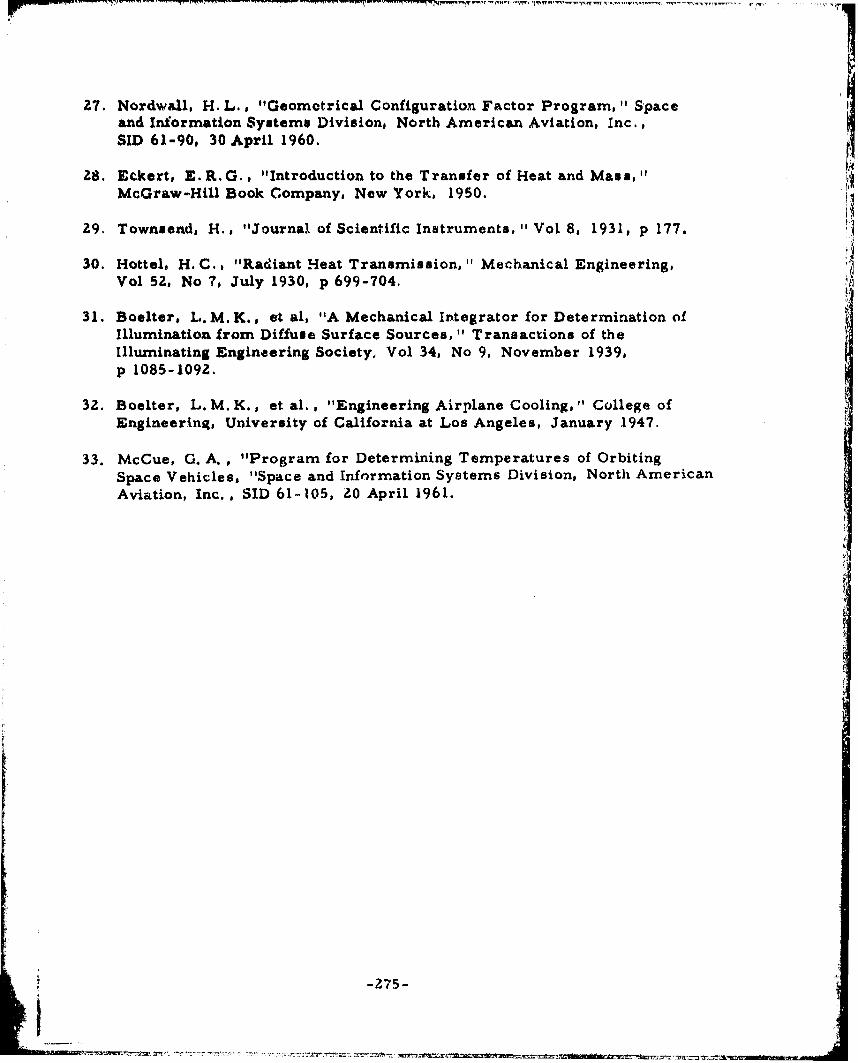
27. Nordwall, H. L., "Geometrical Configuration Factor Program, " Spaceand Information Systems Division, North American Aviation, Inc.,SID 61-90, 30 April 1960.

28. Eckert, E. R.G., "Introduction to the Transfer of Heat and Mass,"McGraw-Hill Book Company, Now York, 1950.

29. Townsend, H., "Journal of Scientific Instruments," Vol 8, 1931, p 177.

30. Hottel, H. C., "Radiant Heat Transmission," Mechanical Engineering,Vol 52, No 7, July 1930, p 699-704.

31. Boelter, L.M. K., et al, "A Mechanical Integrator for Determination ofIllumination from Diffuse Surface Sources, " Transactions of theIlluminating Engineering Society, Vol 34, No 9, November 1939,p 1085-1092.

32. Boelter, L. M. K. , et al., "Engineering Airplane Cooling," College ofEngineering, University of California at Los Angeles, January 1947.

33. McCue, G. A. , "Program for Determining Temperatures of OrbitingSpace Vehicles, "Space and Infrrmation Systems Division, North AmericanAviation, Inc., SID 61-105, 20 April 1961.

-275-

APPENDIX A

TABLES OF EMISSIVITY AND ABSORPTIVITY

This appendix was supplied by the AiResearch Manu-facturing Division of the Garrett Corporation. Thedata presented are incomplete and will be expandedin the first revision of the basic report.

INTRODUCTION

Because radiative heat transfer is a surface phenomenon, it is usuallydesi-able to coat the heat transfer surface to accomplish the desired radia-tivL .xchange. The properties of these surface coatings are of importancein the design of space heat rejection systems, because radiation is the only

means of dissipating heat other than expelling large masses from the vehicle.The radiator may be exposed to radiation from the sun, nearby planets, andother parts of the vehicle.

Considerable work has been done in recent years in developing coat-ings, particularly those which are spectrally selective. Some of theapplications and the desired types of coatings are listed in Table 1.

NOMENCLATURE

a Total absorptivity

Sa Total absorptivity to solar radiation

iaA Monochromatic absorptivity

( •Total emissivity

F -- Total emissivity of radiator surface

C • Monochromatic ermissivity

'Wavelength, microns

. . Microns (1.0 micron = 10 centimeters)

-277-IPoNvious PAGQliRLvo1,

Table 1. Coatings and Their Application

Application Desired Coating Result

Absorber for heat High solar absorptivity, High-energy absorption,engine using solar low thermal emissivity high temperatureenergy

Photovoltaic cell High solar absorptivity High-energy absorption,for cell sensitivity low temperaturerange, high thermalemis sivity

Infrared detector High solar reflectivity, Infrared detection, lowwindow high thermal transmit- temperature

tance

Low-temperature Low solar absorptivity, High heat rejection perradiator high thermnl emissivity unit area

High temperature High thermal emissivity High heat rejection per

(low solar absorptivity unit areadesirable as long as E Tis high)

Solar concen- High solar reflectivity High-efficiency concen-trators trator

Passive tempera- Variable a c to Constant internal tempera-T

ture control accommodate solar flux turesystem and internal heat load

changes

Ultraviolet pro- Reflective or absorbing Reflection or con"-ersiontective coating of ultraviolet into anotherfor organic form to protect organicmate rials mate ra is

SELECTIVE ABSORPTION OR EMISSION

The use of spectrally selective coatings is often desirable to controlenergy flux. There are many materials whose total emissivity varies withtemperature, and these can often be used to achieve the proper energybalance. Figure 1 shows, i.i general, how total emissivity varies with

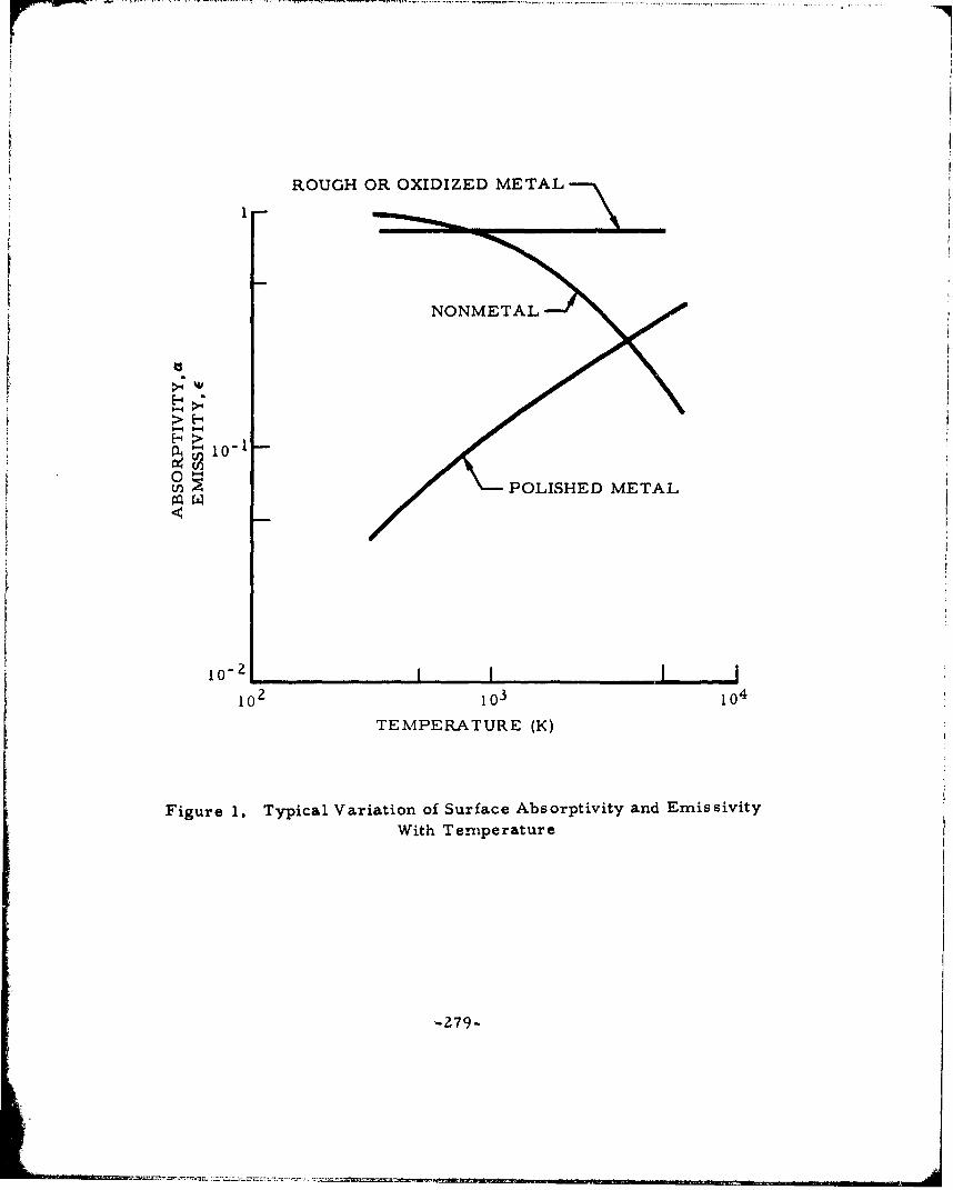
ROUGH OR OXIDIZED METAL

>- H

• 10-1

0~On •-POLISHED METAL

IO-2 III_.. .._I10"2 1 03 104

TEMPERATURE (K)

Figure 1. Typical Variation of Surface Absorptivity and EmissivityWith Tenmperature

-279-

temperature for metals and nonmetals. For example, a.s/T is shown tobe greater than unity for polished metals and less than unity for nonmetals.

By use of the principles outlined in the body of this report, selectiveradiation surfaces can be fabricated by depositing multiple layers of coatingmaterial on the surface. Interference films, cavity absorption, absorbingundercoatings, Fresnel (or dielectric) films can be utilized.

For example, a gold smoke film evaporated from a tungsten filamentin the presence of small amounts of nitrogen and oxygen has the property ofbeing almost completely transparent to radiations above 2 microns. About97 percent is transmitted, whereas only 20 percent of the visible spectrumis transmitted with 2 to 3 percent reflection, using a heat source of 120 F,Reference 1.

A polished copper surface may be assumed to be 75 percent reflectivein the visible and 98 percent in the infrared range. Thus, if the gold smokefilm were deposited on this copper surface, 92 percent of the radiation atove2 microns and only 5 percent of the visible radiation would be reflected dueto the double absorption. However, at elevated temperatures the structureand optical properties of the film is affected and stability becomes a factor.

Because emissivity is strongly dependent on surface characteristics,it is necessary that the surface be, maintained in a condition most closelyapproximating the operating environmental conditions during emissivitymeasurements. In the case of space radiators, high vacuum is mostimportant. Grease, dust, impurities or absorbed gases can materiallyaffect the expected response of a surface.

SPECTRAL CHARACTERISTICS OF COATINGS

The spectral characteristics of some coatings which may be appli-cable for space radiators are given here. The values for total ernissivityare taken from several sources. These totals are only indicative of coatingemissivity, because substrate preparation and method of deposition greatlyinfluences the spectral characteristics.

The spectral characteristics of some enamels and pure oxides areshown in Figures 2 through 7 (Reference 2). These characteristicsare presented as indicative of the type of information which can be foundin the literature.

-280-

i t~.

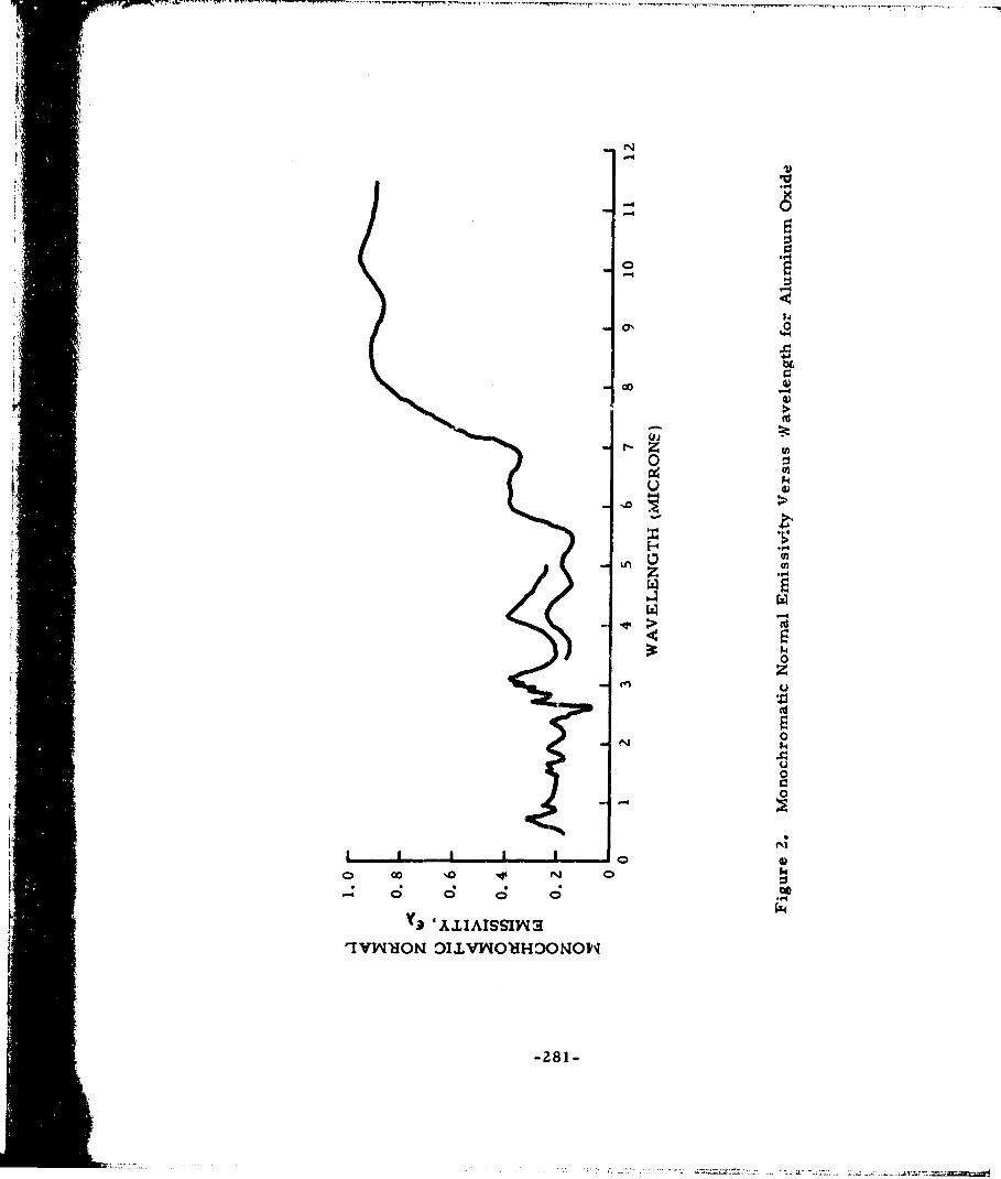
-F4-40

a' 0

U)

('44

o0U)

U 40

H0

0C; CzI(4HO OUuNHOO

-281U

'40

00 >

00?

P~4

-282-

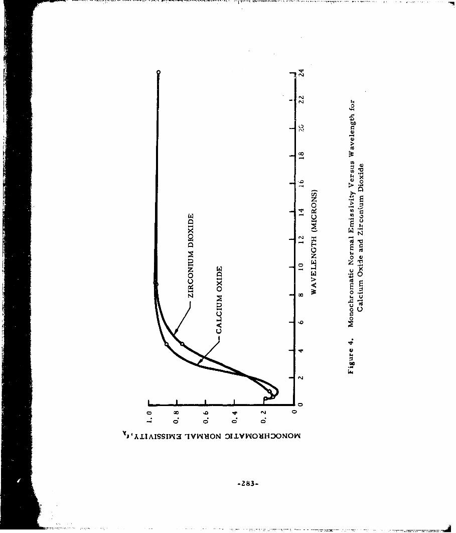
'...'w~~~1.Vu \~~r.. ~~-~fl? '.O'¶ WYX7" r v('~Nrn,.'.OD

z ~0 4

6--4

o. o U

10uZ

.-o

00

NIW'O DIVWOdDO

-283-U

034J

000

oo0 c)

z ~ z"14

00 o

u-zzoN

-24-

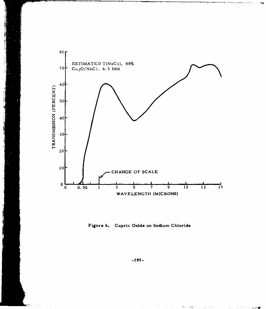
80

ESTIMATED T(NaCI), 88%70 Cu 2 O/NaC1, 6.5 MM

60

z

US50-

z0 40-

ii 30-

zo20 -

CHANGE OF SCALE

"0o 0.50 1 3 5 7 9 11 13 15

WAVELENGTH (MICRONS)

Figure 6. Cupric Oxide on Sodium Chloride

-285-

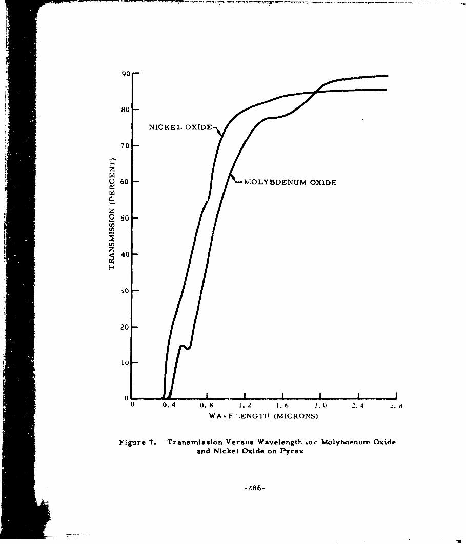
1 !iW¶'l -- -- --~ -.-90

80-

NICKEL OXIDE

70 -

zU 60 - MOLYBDENUM OXIDE

0 50l~ll!

z 40

30

20

.il! i'10 --

I0

0 0.4 0.8 1.2 1.6 2.0 .4 2WAý F>ENGTH (MICRONS)

Figure 7. Transmission Versus Wavelength ioA7 Molybdenum Oxideand Nickel Oxide on Pyrex

-z86-

•--i• =77-

ORGANIC COATINGS

Considerable effort is being directed toward development of organiccoatings with high thermal emittance at -relatively low temperature (fromroom temperature to 200 or 300 F). These coatings must be characterizedby high resistance to ultraviolet and nuclear radiation, good thermalstability, and high molecular weight to minimize boiloff losses. Prelimi-nary work indicates that organic coatings can bo developed with a thermalemissivity greater than 0.95. At the present time, no organic coating canbe recommended which will meet all the environmental requirements. Somework on protective ultraviolet absorbers is producing encouraging results,indicating that a high-emissivity coating which is sensitive to ultraviolet maybe successfully protected. These organic protective coatings include 1, 1'ferrocane dicarboxylic acid, 2(2' hydroxy 51 methyl phenyl) benzotriazoLe,and 2 hydroxy 4 methoxy benzophenone.

INORGANIC COATINGS

Because pure metals are generally reflective at temperatures from100 to 1200 F, they are not suitable for radiator coatings. However, theremay be related components which require high thermal reflectance.Typical reflectivity values for vacuum-deposited gold on flat organicsubstrates are 0.95 for the near and far infrared regions. Aluminum,copper, and silver are also reflective from 0. 90 to 0. 95 for the same"region (Reference 3). Care is required to prevent surface oxidation.

Metallic oxides have relatively high emissivities in the infraredregion and low absorptivity for solar irradiation. The emissivities ofsome coatings as reported by various references are summarized inTable 2, which also lists some of the physical properties.

Information received from other sources and from tests conducted atAiResearch indicate that an emissivity of at least 0.85 at 100 to 200 F careasily be obtained for some of these oxides using flame spraying. Thevalues of 0. 93 to 0. 97 at the low temperatures listed in Figure 1 can beobtained only under ideal conditions.

The dependence of emissivity on temperature for some other mate-rials is given in Figure 8. Sheet 2 of Figure 8 shows that fT will beof the order of 0.8 and 0.9 while a should be in the range 0. 1 to 0. 2. Ifthe coatings are roughened, i T ang a. should both increase.

The emittance of two ceramic coatings prepared by the NitionalBureau of Standards is shown in Figure 9. These coatings are bariumnsilicate glass containing mixtures of quartz, aluminum oxide, chromeoxide, cerium oxide, and other oxides. They are sprayed on stainless steel

-287-

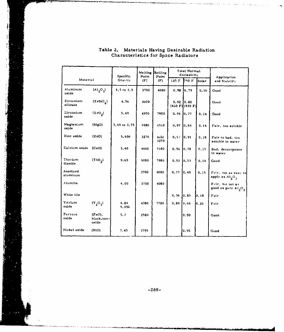
Table 2. Materials Having Desirable Radiation

Characteristics for Space Radiators

Melting Boiling Total Normal |

Specifi. Point Point -T ApplicationMaterial Gra-, ttv (F) (F) 125 F 750 F Solar and Stab, IPx

Aluminum (Al 20 3 ) 3.5 to 3.9 3700 4080 0.98 0.79 0.16 Goodoxide

Zirccnium (ZrSiO4 ) 4.56 4600 0.92 0.80 Goodsilicate (460 F) (930 F)

Zirconium (ZrO2 ) 5.49 4900 7T00 0.95 0.77 0.14 Goodoxide

Magnesaum (MgO) 3.65 to 3.75 5080 6510 0.97 0.84 0.14 Fair, too soluble- oxide

Zinc oxide (ZnO) 5.606 3Z70 subi 0.S/ 0.91 0.18 Fair to bad, too3Z70 soluble in water

Calcium oxide (CaO) 3.40 4660 5180 0.96 0.78 0.15 Bad, decomposesin water

Thorium (ThO2 ) 9.69 5080 7980 0.93 0.53 0.14 Gooddioxide

Anoc~ized 3700 4080 0.77 0.49 0.15 Fair, not as eas\ toaluminum apply as At 20 3

Alumina 4.00 3700 4080 Fpir, bat not asgood as pure A 1 3

White tile 0.96 0.85 0.18 Fair

Yttrium (Y 2 0 3 ) 4.84 4380 7780 0.89 0.66 0.26 Fairoxide 5.096

Ferrous (FeO), 5.7 2580 0.90 Goodoxide black,non-

oxide

Nickel oxide (NiO) 7.45 3795 0.95 Good

-2 88-

co /n 0- N 1 )

/ 00

I '2

.4)

~t t

w P4

.0d -ýa

z -

00,02022 0C0o

0

ý 0, 00 0- 0n 0 00

a;l AISCflN;

-289-

t-

0

0-

0IUU

F F4

00

00

0

(nla

0H/-

N0 N m

-290-

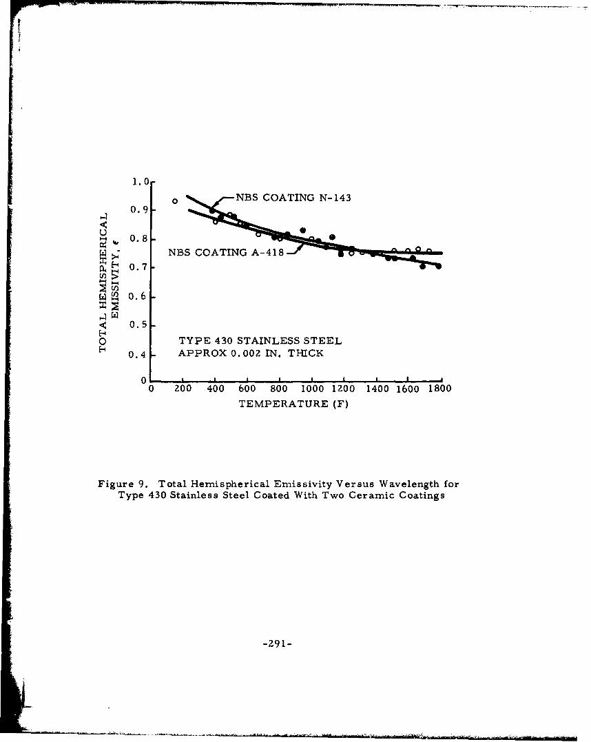
1.0

NBS COATING N-1430.9

U ~, 0.8 -

4 •-NBS COATING A-418•H 0.7

S0.6I-4

.4:: 0.5

0 TYPE 430 STAINLESS STEELH 0.4 - APPROX 0.002 IN. THICK

0 f . I I , I

0 200 400 600 800 1000 1200 1400 1600 1800

TEMPERATURE (F)

Figure 9. Total Hemispherical Emnissivity Versus Wavelength forType 430 Stainless Steel Coated With Two Ceramic Coatings

S~-291-

samples and then cured at elevated temperatures. Most of these coatingsare spectrally selective with a /eT approximately 0. 1 to 0.3, Conservativevalues of emissivities for low-lemperature radiation are of the order of0.85 to 0.90. Higher thermal emissivities are desirable, however, forhigh-temperature radiators such as required for space power systems. Itis believed that for high temperature radiators, black iron oxide or nickel"oxide coating (nickel penetrate) have emissivities near 0.95.

Total normal emissivity characteristics of various materials are shownin Figures 1.0 and 11.

COMPUTATION OF TOTAL EMISSIVITY OR ABSORPTIVITY

The methods used to predict radiation heat transfer require knowledgeof the total emissivities of the surfaces involved as well as the totalabsorptivities. Much of the data published to date are in the form ofmonochromatic reflectivity or absorptivity as a function of wavelength.Thus, it is often necessary to calcuiate the total emissivity or absorptivitywhen only the spectral information is available. Basically, this is done bycalculating the black body characteristics as given by Planckts Law. Theactual power emitted or absorbed is then obtained by taking the product ofthe black body radiant power and the emissivity at each wavelength. Thetotal emissivity is determined by integrating this product over all wave-lengths and dividing by the black body energy over the same wavelengths.

To obtain the value of total emissivity or absorptivity, over all wave-le.ngths ordinarily requires very tedious hand calculations and lengthygraphical integrations. Fortunately, there is available an IBM 7090 programwhich mechanizes the calculation and integration procedures such thataccurate total emissivities and total absorptivities can be obtained veryrapidly for any given temperature conditions and material properties. Thisprogram is titled "Total Emissivity and Absorptivity Program, " and acomplete description of the theory involved and usage of the program isavailable (Reference 7).

-292-

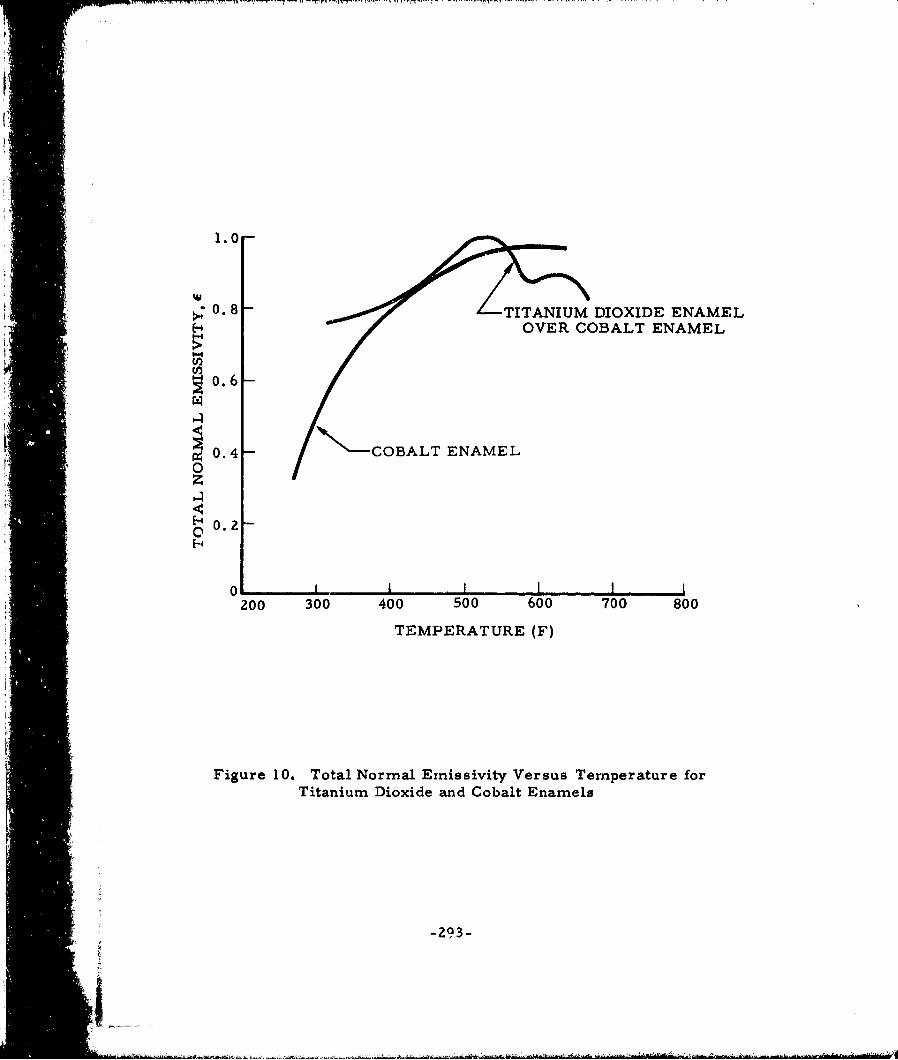
1.0-

0. 8 TITANIUM DIOXIDE ENAMELOVER COBALT ENAMEL

o.6-

0.4- '"K* COBALT ENAMEL

0

4iiii

~0.2

0 l! --- I1.0I

200 300 400 500 600 700 800

TEMPERATURE (F)

Figure 10. Total Normal Emnissivity Versus Temperature forTitanium Dioxide and Cobalt Enamels

-293-

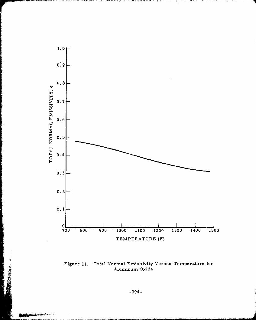
1.0

0.9

0.8

>0.7

•0.6

O 0.5z

0.4

0

0.3

0. 2

0. 1

0 I I I I i i I I700 800 900 1000 1100 1200 1300 1400 1500

TEMPERATURE (F)

Figure 11. Total Normal. Emissivity Versus Temperature forAluminum Oxide

-294-

REF ERENCES

1. Tabor, H., "Selective Radiation: I. Wavelength Discrimination,Transactions of Conference on Use of Solar Energy (Tucson, Arizona),Vol II, Part 1, Section A, October-November 1955.

2. ''A Proposal for the Investigation of Space Heat Rejection Systems forRankine Cycles," AiResearch Manufacturing Company and Electro-Optical Systems, Inc. (Joint Report), 2Z January 1960.

3. Dunkle, R.V., "Spectral Reflectance Measurements, " First Sympo-siumn on Surface Effects on Spacecraft (Palo Alto, California),IZ-13 May 1959.

4. Pirani, M., Journal of Science Institute, Vol 16, 1939, p 12.

5. Coblentz, W.W., U. S. Bureau of Standards, No. 9, 1912, p Z83-324.(A 1203)

6. Sieber, W., Z, Tech. Physik, Vol ZZ, 1941, p 130-135. (MgO)

7. "Total Emissivity and Absorptivity Program, " Space and InformationSystems Division, North American Aviation, SID 61-3, February 1961.

-295-

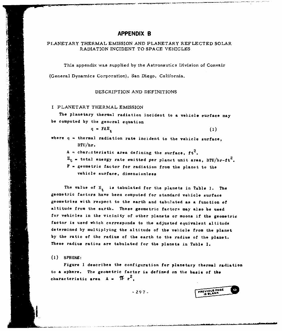
APPENDIX B

PLANETARY THERMAL EMISSION AND PLANETARY REFLECTED SOLARRADIATION INCIDENT TO SPACE VEHICLES

This appendix was supplied by the Astronautics Division of Convair

(General Dynamics Corporation), San Diego, California.

DESCRIPTION AND DEFINITIONS

I PLANETARY THERMAL EMISSIONThe planetary thermal radiation incident to a vehicle surface may

be computed by the general equationq t (1)

twhere q a thermal radiation rate incident to the vehicle surface,

BTU/hr.

A = char.Lcteristic area defining the surface, ft2.

Et= total energy rate emitted per planet unit area, BTU/hr-ft 2.

F geometric factor for radiation from the planet to the

vehicle surface, dimensionless

The value of Et is tabulated for the planets in Table I. The

geometric factors have been computed for standard vehicle surfacegeometries with respect to the earth and tabulated as a function of

altitude from the earth. These geometric factors may also be usedfor vehicles in the vicinity of other planets or moons if the geometric

factor is used which corresponds to the adjusted equivalent altitudedetermined by multiplying the altitude of the vehicle from the planet

by the ratio of the radius of the earth to the radius of the planet.These radius ratios are tabulated for the planets in Table I.

(1) SPHEIRE:

Figure 1 describes the configuration for planetary thermal radiation

to a sphere. The geometric factor is defined on the basis of the

characteristic area A - 1I r2,

-297-

where r to the radius of the sphere. Then

F - ql/* r2 Et

The geometric factor for a sphere with respect to the earth is tab-

ulated in Table 2 as a functiozr of altitude,

(2) CYLINDER

Figure 2 dpscribes the configuration for planetary thermal radiation

to the convex surface of a cylinder. Because of lack of three dimen-

sional symmetry an attitude parameter, , is required and is the angle

between the cylinder axis and the vertical to the vehicle. The geometric

factor is defined on the basis of the characteristic area, A a DL, where

D and L are the diameter and length, respectively, in feet for the

cylinder. Then

F - q/DLEt (3)

The geometric factor for a cylinder with respect to the earth is

tabulated in table 3 as a function of altitude with the attitude angle,

, as the parameter.

(3) HEMISPIIERE

Figure 3 describes the configuration for planetary thermal radiation

to the convex surface of a hemisphere. The geometric factor is defined

on the basis of the characteristic area, A - r , where r is the radius

of the hemisphere. Then

F - q/¶ r 2 Et (4)

The geometric factor for a hemisphere with respect to the earth is

takbulated in Table 4 as a function of altitude with the attitude angle,

9 , as parameter.

-298

(4) FLAT PLATE

Figure 4 describes the configuration for planetary thermal radiation

to one side of a flat plate. The angle. 4 ? between the normal to the

plate and the vertical to the vehicle defines the attitude of the plate

with respect to the planet. The geometric factor is defined on the basis

of the characteristic area, A - P, the area of one side of the plate.

Then

F - q/PEt (5)

The geometric factor for a flat plate with respect to the earth is

tubulated in Table 5 as a function (if altiti,,,e with the attitude angle,

_ ,as parameter.

It should be noted that the flat plate thermal radiation solution

F |may be used to approximate the thermal radiation incident to any generally

convex vehicle surface by dividing the surface into a series of flat plate

elements and summling the thermal radiation incident to each of these flat

plates.

II PLANETARY REFLECTED SOLAR RADIATION

The planetary albedo incident to a vehicle surface may be computed

from the general equation:

q - FASa (6)

where q - albedo heat flux rate incident to the vehicle surface, BTU/hr.

A - characteristic area defining the surface, ft 2

S - solar heat flux or "constant", BTU/hr.-ft 2

a - average reflectivity of the planet's surface, dimensionless

F . geometric factor which accounts for reflected energy distribution

on the planetary surface and the geometry, dimensionless

The geometric factor for a sphere is independent of attitude due to

-299-

three dimeunional syimetry. In the case cf all surfaocem the loCatiiti of

the vehicle with reslpec t to) the sun is defi ,,i !d by the zenith dis tance

between the surface and sun, 8S The zeni th dis tance is the angle

between the earth-vehicle vector auii the earth-sun vector. In the case

of surfaces lacking spherical symmetry, the attituide of the surface is

defined by two angles. One is the angle. oA , between the axis of the

cylinder or hemisphere or normal to the flat plate and the vertical to

the vehicle. The other is the angle,?0 , of rotation of the axis or

normal about the vertical to the vehicle from the plan(2t. The datum

0 - U occurs when the axis or normal lies in the plane defined by

the earth-vehicle vector and the earth-sun vector,

The value of S and a are tabulated for the planets in Table I.

The geometric factors for albedo have been computed for standard vehicle

surface geometries with respect to the earth and tabulated as a function

of altitude from the earth. Again, as described for th,!rmal radiation,

these geometric factors ma., be applied to other planets by using, the

ratio of the radius of the earth to the radius of the planet tabulated

in Table 1.

(1) SPHEREFigure 5 shows the configuration for albedo incident to a sphere.

The geometric factor is defined on the basis of the chauracteristic ar;a,A • r2

A r r , where r is the radius of the sphere, then

F W q/lrr2Sa (7)

The geometric fac+or for albedo incident to a sphere from the

earth is shown in Table 6 as a function of altitude in nautical miles

with zenith distarce, O, as parameter.

(2) CYLINDER

Figure 6 shows the configuration for albedo to the convex surface

of a cylinder. For a cylinder the geometric factor is defined on the basis

-300 -

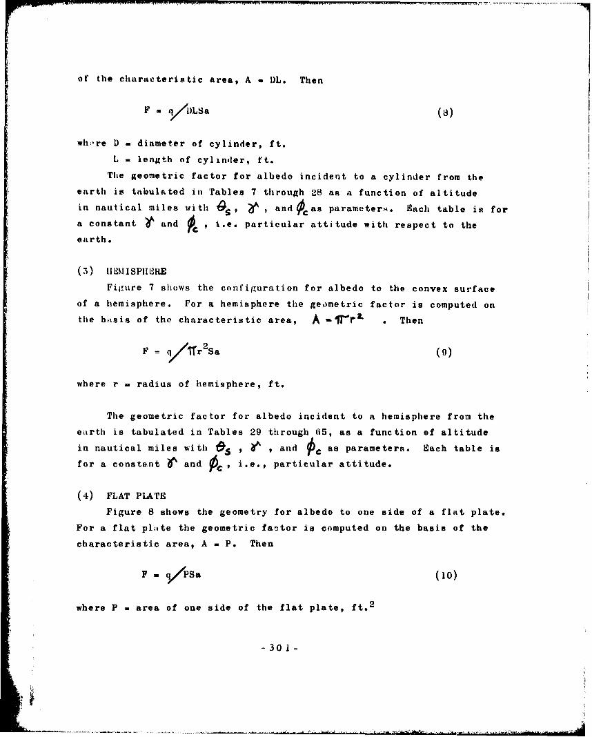
of the characteristic area, A . DL. Then

F m q/'DLSa 03)

wh.ure 1) - diameter of cylinder, ft.

L - length of cylinder, ft.

The geometric factor for albedo incident to a cylinder from theearth is tabulated in Tables 7 through 28 as a function of altitude

in nautical miles with Os, , and Aas parameter.. Each table is for

a constant and , i.e. particular attitude with respect to thefC

earth.

(') I "ý IIS P II R E

Figure 7 shows the configuration for albedo to the convex surface

of a hemisphere. For a hemisphere the geometric factor is computed on

the basis of the characteristic area, A -¶TrL . Then

F = q/TIr 2 Sa (9)

where r - radius of hemisphere, ft.

The geometric factor for albedo incident to a hemisphere from the

earth is tabulated in Tables 29 through 65, as a function of altitude

in nautical miles with U 5 ' , and OC as parameters. Each table is

for a constant and %, i.e., particular attitude.

(4) FLAT PLATE

Figure 8 shows the geometry for albedo to one side of a flat plate.

For a flat plate the geometric factor is computed on the basis of the

characteristic area, A - P. Then

F - q/PSa (10)

where P = area of one side of the flat plate, fto 2

-301-

Tlho geometric factor for albedo incident to one side of a I'Iit plte

from the earth is talpi~Jitud in Tabbles (01 througeh l ]11 aaa funl Lion of

I, ti tude in nautical mi I S with , &ald Ocas parameters. &'Iich t'AhI

is for a consLant r and Af i.e., pnrticular attitude.

The flat plate ulbedo solution may also be used to approximate

,.lh?,do henLci•.g of any goriernIly con-vex satellite or satellite surface

by dividing this s:irface into a series of flat plates and summing the

albedo heating for ench of these flat plates.

- 30 2-

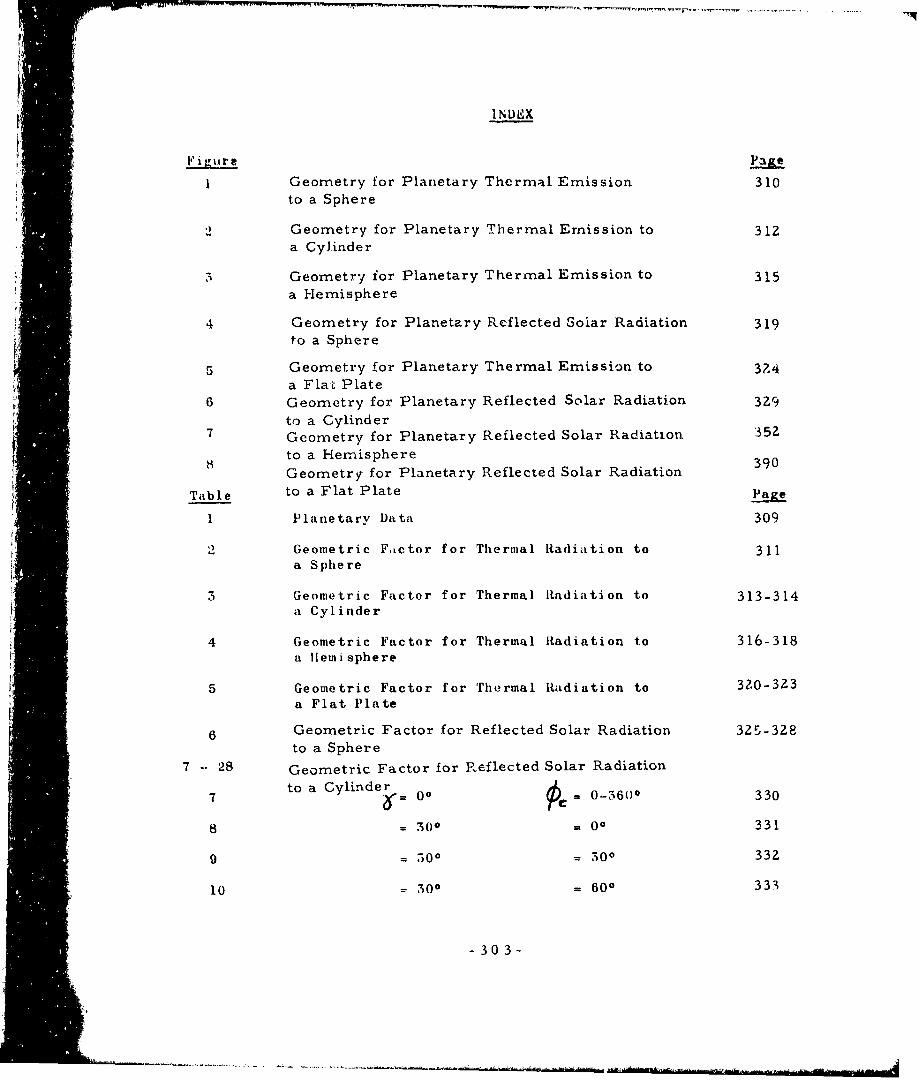
1ND1EX

F igura

1 Geometry for Planetary Thermal Emission 310to a Sphere

2 Geometry for Planetary Thermal Emission to 312a Cylinder

Geometry for Planetary Thermal Emission to 315

a Hemisphere

4 Geometry for Planetary Reflected Solar Radiation 319

2 to a Sphere

a Geometry for Planetary Thermal Emission to 374

a Flat Plate6 Geometry for Planetary Reflected Solar Radiation 3Z9

to a Cylinder7 Geometry for Planetary Reflected Solar Radiation 352

to a HemisphereGeometry for Planetary Reflected Solar Radiation 390

Table to a Flat Plate

1 Planetary Data 309

2 Geometric FLctor for Thermal Radiation to 311a Sphere

3 Geometric Factor for Thermal ltadiation to 313-314a Cylinder

I4 Geometric Factr for Thermal Radiation to 316-318

* ~a Iletni sphere

5 Geometric Factor for Thermal Radiation to 3Z0-3Z3

a Flat Plate

6 Geometric Factor for Reflected Solar Radiation 325-328to a Sphere

7 -- 28 Geometric Factor for Reflected Solar Radiation

to a Cylinder 0"_7 00' 0I-= 0-3600 330

8 = 300 = 00 331

9 =500 = 30o 332

10 3 ,00 = 600 333

-303-

. . . .. .. .---

INDIAX (CIINi'.i!rable-_ 500 = 900 334

12 = 300 = 1210° 335

13 = 7,0 = 1500 336

14 = 300 = 180° 337

15 = 600 = 00 338

16 = 6- 300 339

17 60° = 60° 340

18 = 600 = 900 341

19 = 600 = 1200 342

)0 - 600 =1500 343

S 21 = 600 = i8o0o 344

22 =900 = 00 345

23 = 90° = 50° 346

24 = 900 = 6(0 347

25 = 900 = 900 34826 = 900 = 1200 349

27 = 900 = 1500 350

28 = 900 = 1800 351

29-65 Geometric Factor for Reflected Solar to a Hemisphere

29 = 00 00-3600 353

30 = 300 00 354

51 = 300 = 300 355

52 = 300 = 600 356

35 = 330 = 900 357

54 = 500 = 1200 358

55 w 300 = 1500 359

- 304-

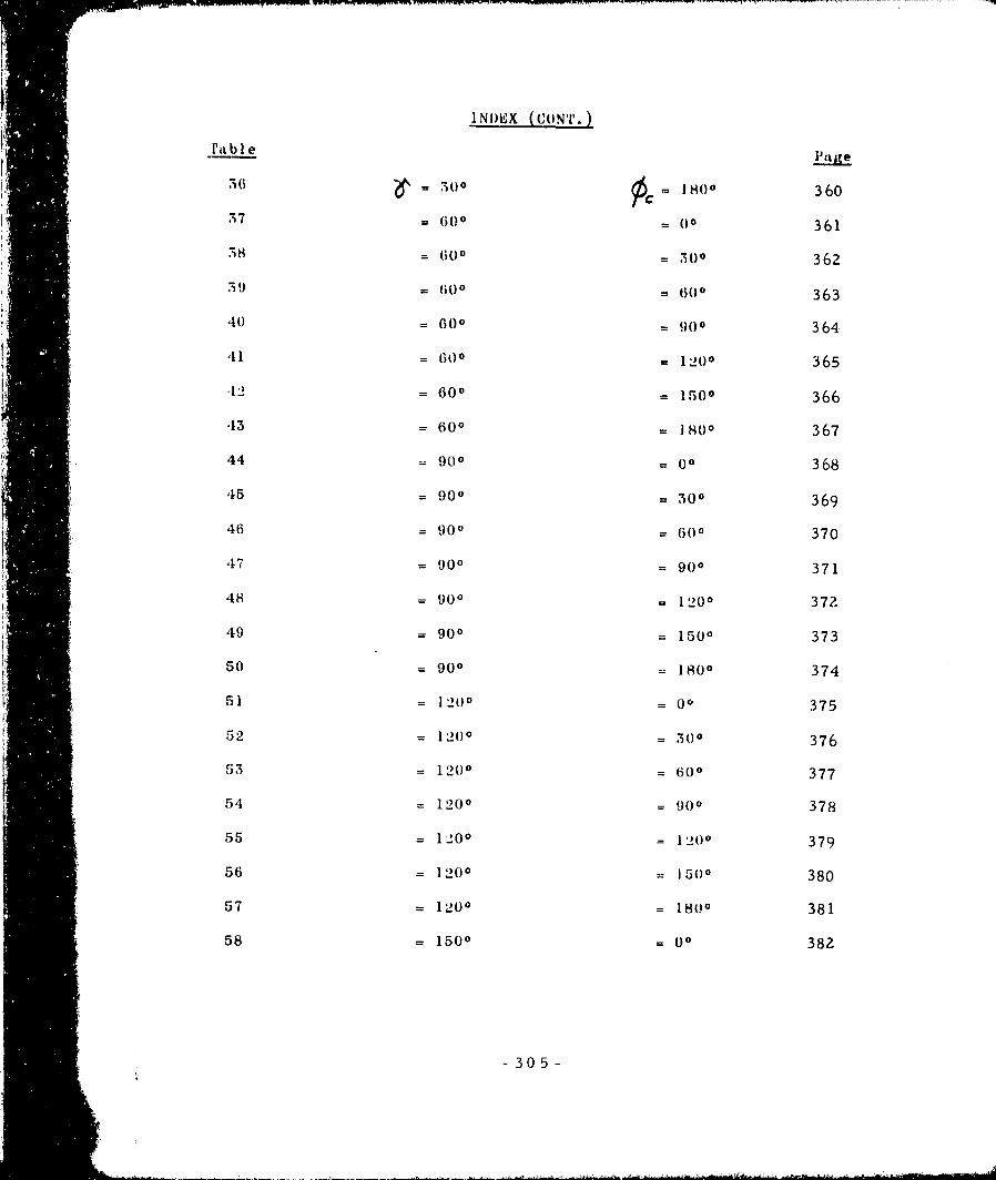
1NDEX (CONT.)

06 3 I80- = 510 = 1 360

57 6(0 361

"a58 - 600 = 3)0 362

09 = 600 = 600 363

40 = 600 = 900 364

41 = (100 = 1200 365

-12 = 600 = 1500 366

45 = 600 = 180 0 367

44 = 900 = 00 368

45 = 900 = 300 369

46 = 900 = 600 370

47 = 900 = 900 371

48 = 900 = 1200 372

49 = 900 = 1500 373

50 = 900 = 1800 374

51 = 1200 = 00 375

52 = 1200 = 300 376

53 = 1200 = 600) 377

54 = 1200 = 900 378

55 = 12200 - 1200 379

56 = 1200 = 1500 380

57 = 1200 = 1800 381

58 = 1500 = 00 382

-305 -

I ND 1EX C 0NT

1'dable

59 1500 3, 0 0 383

60 = 1500 600 384

61 = 1500 900 385

(62 = 1500 1 !2(00 386

63 1500 1500 387

64 = 1500 = 1800 388

65 = 1800 = (;G -?.(30 389

66-101 Geometric Factor for Reflected Solar to a Flat Plate

66 o- 0 c= (00-360 391

67 = 500 - 00 392

08 = l0 = 500 393

69 = 500 = 600 394

70 = 50 (0 395

71 = 500 = 1200 396

72 = 500 = 1500 397

75 = 300 = 180)0 398

74 = 601 = 00 399

75 = 60° = 300 400

76 = 6O0 = 600 401

77 = 600 o= 900 402

78 = 600 = 1200 403

79 = 60° = 1500 404

80 = 600 = 1800 405

81 = 9(00 = 00 406

82 = 900 = 300 107

83 = 900 = 600 408

84 = 900 = 900 409

30 6 -

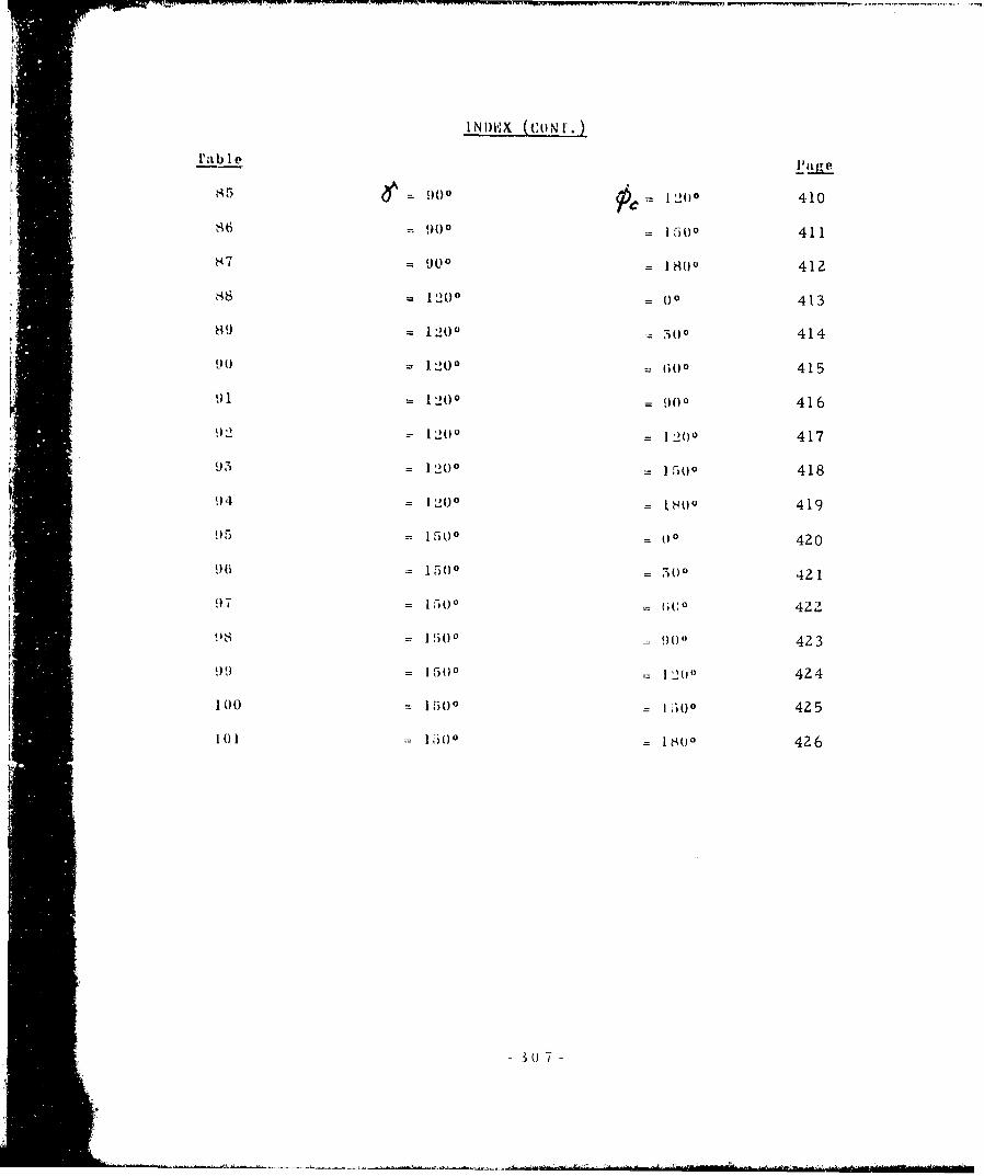
I~ N 1)- NA -' N I-

t•IIrabt I, e I

85 0- 1200 410

86 = 900 = 1500 411

87 = 900 = 1800 412

= 1200 - 00 413

=89 1200 300 414

9) = 1200 = (= )O 415

91 = 1200 = 900 416

0 2 1- =20 1 2)00 417

93 = 1200 = 150) 418

94 = 1200 = k 800 419

9) 5 = 1'500 = 00 420

"9 6 = 1500 = 3)00 42 1

97 = 1500 = G Co, 422

U= 150I !)= ) 423

15 0 = 1 2001 424

100 = 15 00 = 13)0 425

10= 1500 = 1800 426

30 7

8 $

:4,0) 0 .

'0p 0' CK N ,-0 L'\ 0H00%C- aA4

0 i

0u 4O ' a o ) 1-H rk- %40 4 0' 0 H~CO~L

43G

0 L~

4-2

_ H 4

9 ýo (; _ g 4 -41

0 0 P

H1 4) 4.3

1: ON co C- 4Ax1 I CO 43, ss 0H 04.7.

0 0 S 0 0 0 0N09 0 HH H Uri O' '. 0 0pH

H~~ 4.11 430- i

m CN 0

L2\LAA

-39 SRV~U HA

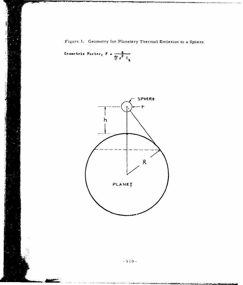
Figure 1. Geometry for Planetary Thermal Emission to a Sphere

Geometric Factoro FTr2fr E t

$ PH C Re

PLANET

3 10 -

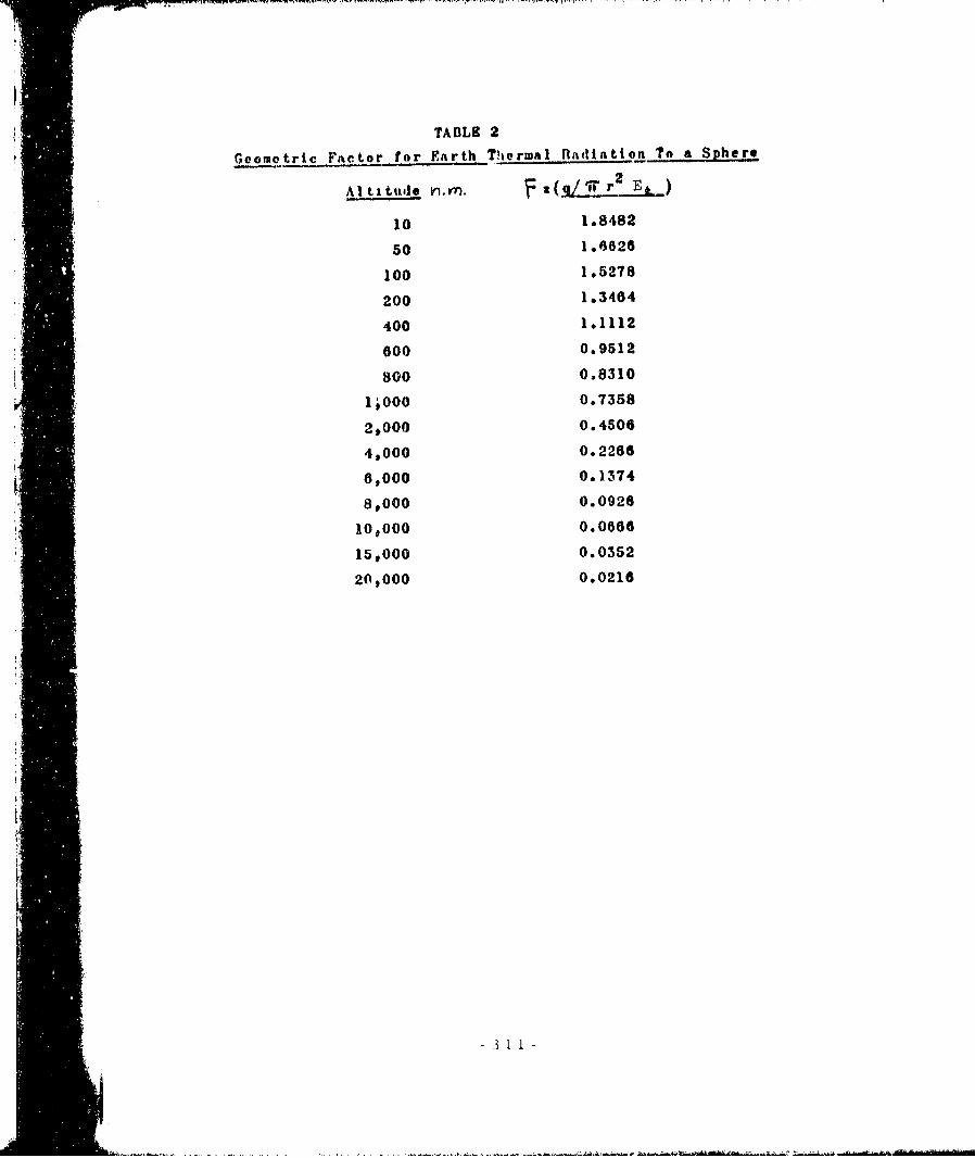
TABLE 2

Geometric Factor for Earth Thermal Radiation To a Sphere

AI t i tude vi. . q/ I r2___-=)

10 1.8482

50 1.6626

100 1.5278

200 1.3484

400 1.1112

600 0.9512

800 0.8310

1;000 0.7358

2,000 0.4506

4,000 0. 2266

6,000 0.1374

8,000 0.0926

10;000 0.0666

15,000 0.0352

20,000 0.0216

3 [ 1 -

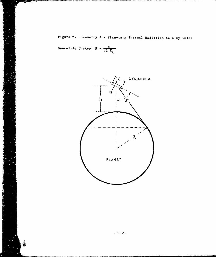
Figure 2. Geometry for Planetary Thermail Radiation to a Cylinder

Geometric Fa&ctor, F qbDL E

t

A./ LICW 0LINDp,

PLANETf- 2-

N ) -4( (2) cl 00t-7) 0- U')4 4~ 40 0co b t 0 -t-CO r l t w it 40V I r00000 l-4It O~ " t- N0

64 ~ 00000 00000 000 000

4a to to! 00000o 00004 00 00 000000 00000004d P-4 .-eI P4r V4r- -

N 84 t-NV 00 0"1 O &a t 40000 - D0 -

04

0 0 ;-

o~~~~~~~~ 1J 3 0 0 0 0 0 0 0 0 0

a V 00 00 to 0 00, - 0 " 0 go P

C30

4A 4

1-4I~ 00 000Dp000 -0 toC3000 0 c nont e

.0

01

0 0 0 00000 000000000c 0C

48 IV ar 0000000vW0 o4 0 0g 0 0 0 0 tg G 0 00 0 0

.93 1

Figure 3. Geometry for Planetary Thermal Emission to a Hemisphere

Geometric Factorg F -

S2r Et

P ANET

-31 5

o~ 1 - ") m CAV w CA.~0 C's " 0u fol 0f)o ' c CAv c 03t- t4JLn-vv 0 A ca 0o o 0 00 -. g C C 0

CD~0** 0 a o o o S0 c; 49 *; c; 0 S

-4 tJ 00LO00 'lIVt0 0-4ell vOto000 00Av 00oc000000t f

at

5. 4~ Ga,4 0000 0000000000C (0000000000

G) a ý t .1t -c l Q- -* t-- -0 0 4 V. CAI 0 t- P

o as ot e AC ) - V e AC - 0t

4 J )4-b V

4- $3 -4S 4P4r4p qF4ý 4 L nt )0 w t 2tr- -.. 0 1""- U *

.- ~ ~~~~~ 1 00 0 0 0 0 0 0 0 0 0 0 0 0

-) t0 CI it -~ -t % 0 C I t -t

0f00 00 A00000000 00 000000'0

44 01

I.V .' i.1 0 00 0 00~0 000000 00

ii 0000

0 0

000

!!!!!

F4.

r14

0 CO0 0- w. ,"•.,o t-,tM04 ,, v 0-,• -, 0 P P-4,,CAo0" on-

14 04--v r

0

•m •I 0 O00 00000000•0O 00 ac00C300

S.,,.• 0 0 00 0 0 C',000

31.• o~

i- •~~~ ~ I ooIoooooooooo~o

.- .000•P0000000 0000000000 00000

4.0 00000 00000 00'•- !!000

,, • m 7-m

tj00000 0000000000

L~ 00000 0000000000

tj l 04 000to00 00 v00Go000000t C

w, .41 CA P- - 4 - -4 r-4 0-4 0 4 -

£ 4 34

O - 0 *0 00 0000000000; ý c c

0.-co

$4£

4u 0-4 )0 0 000 00 0 0 0 0 000200

ti 0

E

CI4 E1 £ 0000000000o 00000c>0000 00000

4.P4

Figure 4. Geometry for Planetatry Thermal Rtadiation to a Flat I'1ftto

qGeome'tric Factor, F PE

FLAT PLATE

A'SEA P

14o2- MAL

PLANET

3 319 -

01 q'O-P4tI o01eqvL)4 -o ota j n n l00tIt 0 4"0t

40 40 lr4r4 v 0

w- to r-o )t jt -0 b0r4e nVU

040

to~~ 0- 93 "0 P0 04 0" P4 0- * P4 0 0 " 0- 0. r. P- r- 0- r"P-

j~I.0~~~~ ~ ~ ~ 320-* ý nM0 -

El .rt t~o-e- a -0 0 0t I1A 0 Int €0 0 0 0 0 M 0 00 V0SO to 0'-0," .0 .•0 a t-l 0) 0mJ v vr CA" €l.,. O

CI On V~ to0 c t0 0o m0t .00 0 0 ~~~~~~~P 0- 41 0~-4cani F"io .. r4 F"

04

P4.

FOS

344

10 u

00 0 . . 0 0 e 0 30 0 0 0e aCO OC C' at0

*04

1 4

r

3 2

'S •Soo o Uoo ~ o o o

o S

.4- III, ,,4IIit- •

ooooo ooooo oooooo o coo

-321-

41 0800 p.Cj00 cq ci ej N 0-0-0t0 O "r-" vm "",

in V* 10 QCIJ es 4.-40 0 00 C)01C~Ij P4 f4 01 0)0 )000

04 .9 C:-- s4

43

cd 0 *L

P- r0 0 w~ 0 0 0 0 0 00 0 00000000000

9.414

423 2 2

0000000000 0 Ci 00QC 0

v 04 40.4 . S

044.1

d

-.4 M- 00 0 0 0 0 o 0 0 0 04.~~o 03P~~ CJJ4ClCA C')C41

ca

A 0'

4a

00CIO0SOSO0I0t'00 C)4

133 2 3

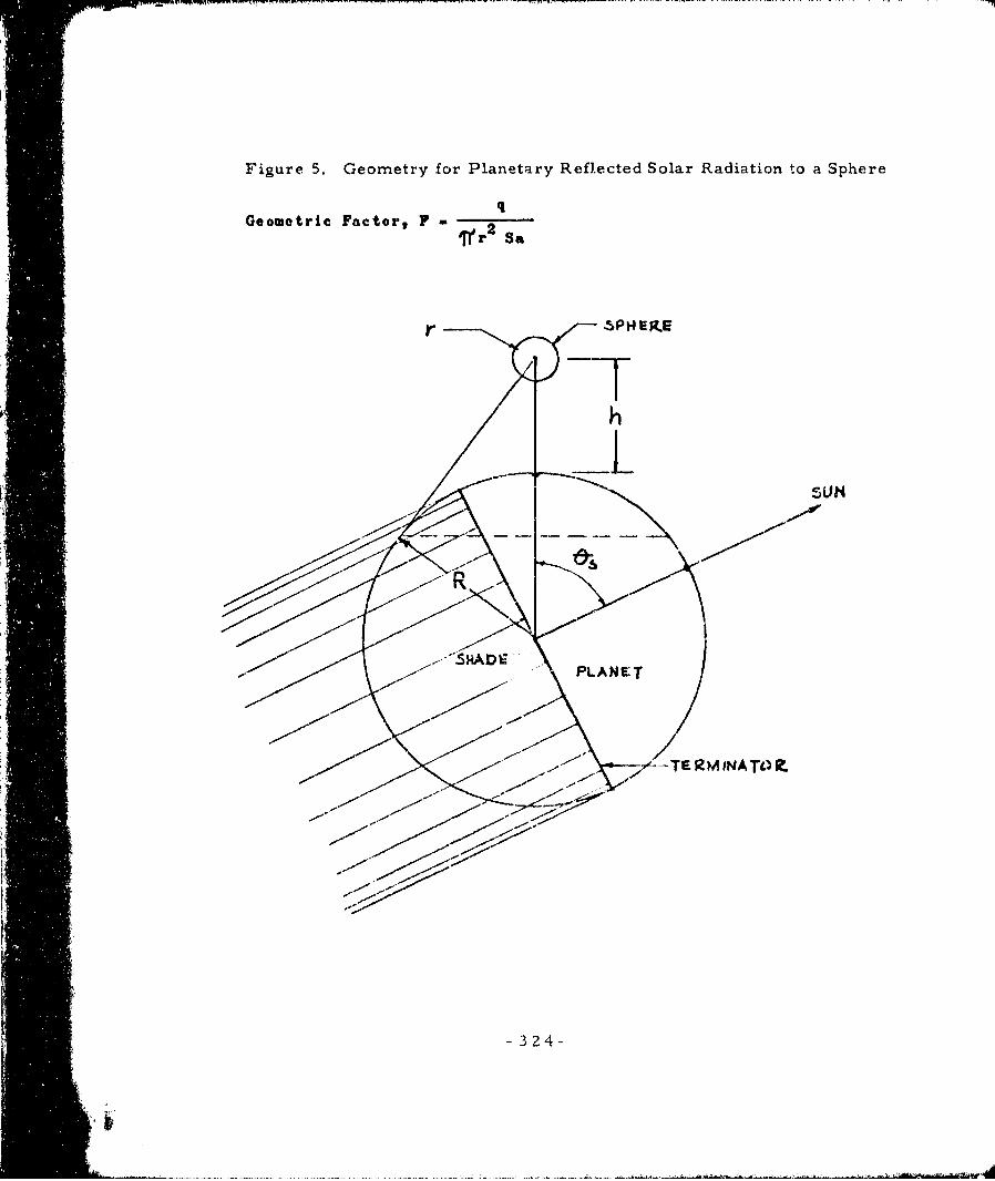
Figure 5. Geometry for Planetary Reflected Solar Radiation to a Sphere

qGeometric FactorT--•r2 S2

Sr- /PHElsE

SUN

• -W .• *" PLANET

-3-TERM-INA TOI

-324-

Table 6, Geometric Factor for Reflected Solar Radiation to a Sphere

Altitude - Altitude Gs FD. me degrees O. no degrees

50 0 1.6661 200 0 1.339350 10 1.8408 200 10 1,3190s0 20 1.5656 200 20 1,258550 30 1.4429 209 30 1.130950 40 1.2763 200 40 1.028050 50 1.0710 200 50 0o060950 80 0.8331 200 60 0.8697s0 70 0.5898 200 70 0.458050 80 0.2893 200 80 0.233450 85 0.1454 200 85 0.123150 88 0.0609 200 88 0.064950 90 0.0152 200 90 0.0358

200 100 0.001780 0 1.5757

8o 10 1.5518 500 0 1.007080 20 1.4807 500 10 0.991780 30 1.3646 500 20 0,9463

40 1.2071 500 30 0.8721

80 50 1.0129 500 40 0.771480 60 0.7879 500 50 0.647380 70 0.5389 500 60 0.503580 80 0.2736 500 70 0.344880 85 0,1383 500 80 0.181880 88 0.0609 500 85 0.108080 90 0.0209 500 88 0.071380 100 0. 0003 500 90 0.0516

500 100 0.0070100 0 1.5269100 10 1.5027 800 0 0.8053100 20 1.4339 800 10 0.7931100 30 1.3215 800 20 0.7568100 40 1.1689 800 30 0.6974100 50 0.9808 800 40 0.6169100 60 0.7630 800 50 0.5177100 70 0.5219 800 60 0.4027100 80 0.2650 800 70 0.2772100 85 0.1346 800 80 0.1527100 88 0.0613 800 85 0.0986100 90 0.0241 800 88 0.07141 00 100 0. 0005 800 90 0.0581

800 100 0,0129

-325-

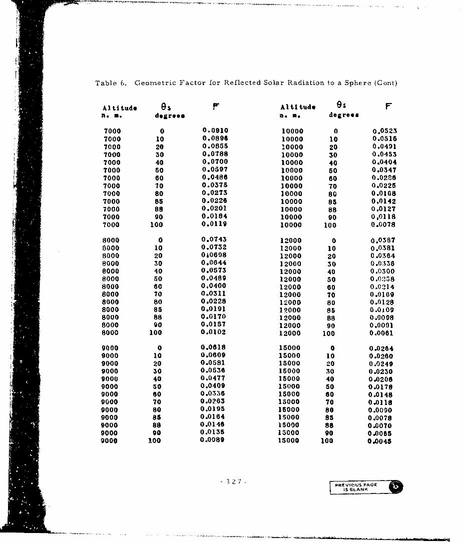
Table 6. Geometric Factor for Reflected Solar Radiation to a Sphere (Cont)

Altitude 95 P Altitude 05 FIt.* . degrees n. Me degrees

7000 0 0.0910 10000 0 0.05237000 I0 0.0896 10000 10 0.05157000 20 0.0855 10000 20 0.04917000 30 0.0788 10000 30 0.04537000 40 0.0700 10000 40 0.04047000 50 0.0597 10000 50 0.03477000 60 0.0486 10000 60 0.02867000 70 0.0375 10000 70 0.02257000 80 0.0273 10000 80 0.01687000 85 0.0226 10000 85 0.01427000 88 0.0201 10000 88 0.01277000 90 0.0184 10000 90 0,01187000 100 0.0119 10000 100 0.0078

8000 0 0,0743 12000 0 o.03878000 10 0.0732 12000 10 0.03818000 20 0.0608 12000 20 0.03648000 30 0,0644 12000 20 0.03368000 40 0.0573 12000 40 0.03008000 40 0.0489 12000 50 0.03588000 60 0.0400 12000 60 0.0214

8000 70 0.0311 12000 70 0.01698000 80 0.0228 12000 80 0.01288000 85 0.0191 12000 85 0.01098000 88 0.0170 12000 88 0.00988000 90 0.0157 12000 90 0.00018000 100 0.0102 12000 100 0.0061

9000 0 0.0618 15000 0 0.02649000 10 0.0609 15000 10 0.02609000 20 0.0581 15000 20 0.02499000 30 0.0536 15000 30 0.02309000 40 0.0477 15000 40 0.02069000 50 0.0409 15000 50 0.01789000 60 0.0356 15000 60 0.01489000 70 0.0263 15000 70 0.01189000 80 0.0195 15000 80 0.00009000 85 0.0164 15000 85 0.00789000 88 0.0146 15000 88 0.00709000 90 0.0135 15000 90 0.00659000 100 0.0089 15000 100 0.0045

-327- 7REv'usN

F Rv osFG

Table 6. Geometric Factor for Reflected Solar Radiation to a Sphere (Cont)

AI ti tud4 0 Fn. mo degree

18000 0 0.019218000 10 0.018918000 20 0.018118000 30 0.016718000 40 0.015018000 50 0.013018000 60 0.010918000 10 0.008818000 80 0.006818000 85 0.005818000 88 0.005318000 90 0.004918000 100 0.0034

328

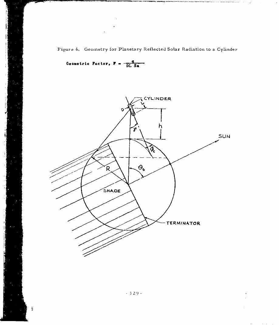
Figure 6. Geometry for Planetary Reflected Solar Radiation to a Cylinder

Geometric Factor, F DL Sa-

r- CYLINDER

•-T

TERMINATOR

3 .

-329

Table 7. Geometric Factor for Reflected Solar Radiation to a Cylinder

0(vertiCAI), -0 -3000

Altitude E~-F k1titude '93 Fn. m. degrees n.o . degrees

100 0 1.1180 1000 70 0.1308100 20 1.0487 1000 80 0.0766100 30 0.9665 1000 85 0.0540100 40 0.8549 1000 90 0.0354100 50 0.7174 1000 95 0.0212100 60 0.5580 3000 0 0.0951100 70 0.3817 3000 20 0.0896100 80 0.1910 3000 30 0.0827100 85 0.0986 3000 40 0.0733100 90 0.0206 3000 50 0.0619100 95 0.0016 3000 60 0.0495300 0 0.7974 3000 70 0.0371300 20 0.7493 3000 80 0.0260300 30 0.6905 3000 85 0.0211300 40 0.6108 3000 90 0.0166300 50 0.5125 3000 95 0.0127300 60 0.3987 6000 0 0.0260300 70 0.2719 6000 20 0.0245300 80 0.1389 6000 30 0.0227300 85 0.0787 6000 40 0.0202300 90 0.0336 6000 50 0.0173300 95 0.0100 0000 60 0.0143600 0 0.5527 6000 70 0,0113600 20 0.5199 6000 80 0.0085600 30 0.4704 6000 85 0.0073600 40 0.4244 6000 90 0.0061600 50 0.3565 6000 95 0.0050600 60 0.2772 10000 0 0.0082600 70 0.1898 10000 20 0.0077600 80 0.1037 10000 30 0.0071600 85 0.0667 10000 40 0.0064600 90 0.0378 10000 50 0.0056600 95 0.0182 10000 60 0.0047

1000 0 0.3723 10000 70 0.00381000 20 0.3504 10000 80 0.00301000 30 0.3232 10000 85 0.00261000 40 0.2861 10000 90 0.00221000 50 0.2404 10000 96 0.00191000 60 0;1873

3 -30-

&,

Table 8. Geometric Factor for Reflected Solar Radiat:ion to a Cylinder

e= 30", D. O"

Al ti tude 011- F AlIt itude 9-n. w. degree@ n. a. degrees

100 0 1.1311 1000 70 0.1251

100 20 1.0601 1000 80 0.0628

100 30 0. 9755 1000 85 0.0386

100 40 0.8613 1000 90 0.0218

100 50 0.7208 1000 95 0.0116100 60 0. 5585 3000 0 0.1462

100 70 0. 3792 5000 20 0.1312100 80 0. 1881 3000 30 0.1173100 85 0.0914 3000 40 0.1003

100 90 o. 0153 3000 50 0.0804100 95 o. 0012 3000 60 0.0595

300 0 0. 8453 3000 70 0.0396

300 20 0. 7882 3000 80 0.0230300 30 0. 7231 3000 86 0.0165300 40 0. 6360 3000 90 0.0114300 50 0. 5296 3000 05 0.0076300 60 0. 4072 6000 0 0.0578300 70 0. 2716 6000 20 0.0518300 80 0. 1300 6000 30 0.0464300 85 0. 0664 6000 40 0.0397300 90 0. 0232 6000 50 0.0324300 95 0. 0068 6000 60 0.0248600 0 0. 6052 6000 70 0,0178600 20 0. 5607 6000 80 0.0118600 30 0. 5125 6000 85 0.0093600 40 0. 4486 6000 90 0.0071600 50 0. 3712 6000 95 0.0054600 60 0. 2824 10000 0 0.0260600 70 0. 1853 10000 20 0.0235600 80 0..0901 10000 30 0. 0212600 85 0. 0510 10000 40 0.0184600 90 0. 0245 10000 50 0.0153600 95 0. 0109 10000 60 0.0122

1000 0 0. 4325 10000 70 0.00921000 20 0. 3973 10000 80 0. 00651000 30 0. 3613 10000 85 0.00541000 40 0. 3143 10000 90 0.00441000 60 0. 2577 10000 95 0.00351000 60 0, 1930

-331-

-!,

Table 9, Geometric Factor for Reflecteýd Solar Radiation to a Cylinder

6~300, 30'

Al ti tude -&3F Al ti tta4 0.3 Fa., . degrees$M a. s* degrees100 0 1.1311 1000 70 0.1288100 20 1.0605 1000 80 0.0864100 30 0.9761 1000 85 0.0419100 40 0.8620 1000 90 0.0245100 so 0.7217 1000 95 0.0135100 80 0.5959 3000 0 0.1463100 70 0.3802 3000 20 0.1322100 80 0.1892 3000 30 0.1189100 85 0.0924 3000 40 0.1020100 90 0.0161 3000 s0 0.0824100 9b 0.0013 3000 60 0.0817300 0 0.8453 3000 TO 0.0419300 20 0.7890 3000 80 0.0252300 30 0.7243 300C 85 0.0185300 50? 04637.5 3000 90 0.0132

30 004314 3000 95 0.0091300 00 0.4092 6000 0.0578300 70 0.2738 6000 20 0.0522300 s0 0.1324 600030046300 85 0 0687 60030 0.0404

300900.0506000 40 0.04042300 95 0.0074 6000 60 0.0257600 0 0.6054 6000 70 090187600 20 0.5621 6000 80 0.0126600 30 (0.5144 8000 85 0.0100600 40 04510 6000 90 0.0079800 50 0.3739 0000 95 0.0080600 60 0.2855 10000 0 0.02,61600 70 0.1836 10000 20 0.0237600 80 0.0934 10000 30 0.0214600 85 0.0540 M00O 40 0.0187600 90 0.0289 10000 50 0.015.600 95 0.0123 10000 s0 0.0125

103CA0 0 0.4327 10000 70 0.00951000 20 0.3988 10000 80 0.00.81000 30 0.3634 10000 85 0.00561G00 40 0.3169 10000 g0 0.00461000 50 0.2607 10000 95 0.00371000 60 0,,964

-332-

Table 10. Geornetric Factor for Reflected Solar Radiation to a Cylinder

S- 30", A 60o

Altitude - Al ti tudo F

n.o . degrees n. m. degreee

100 0 1.1311 1000 70 0.1386

100 20 1.0615 1003 80 0.0759

100 30 0.9776 1000 86 0.0505

100 40 0.8639 1000 90 0.0314

100 50 0.7240 1000 95 0.0182

100 60 0.5620 3000 0 0.1466

100 70 0.3830 3000 20 0.1348

100 80 0.1920 3000 30 0.1226

100 85 0.0953 3000 40 0.1067

100 90 0.0181 3000 50 0.0880

100 95 0.0014 3000 60 0.0678

300 0 0.8453 3000 70 0.0480

300 20 0.7912 3000 80 0.0309

300 30 0.7276 3000 85 0.0237

300 40 0.6418 3000 90 0.0178

300 50 0.5365 3000 95 0.0129

300 60 0.4149 6000 0 0.0579

300 70 0.2800 6000 20 0.0532

300 80 0.1387 6000 30 0.0484

300 85 0.0748 6000 40 0.0423

300 90 0.0294 6000 50 0.0353

300 95 0.0087 6000 60 0.0280

600 0 0.6062 6000 10 0,0210

600 20 0.5660 6000 80 0.0147

600 30 0.5197 6000 85 0.0120

000 40 0.4575 6000 90 0.0096

600 50 0.3815 6000 95 0-0075

600 60 0.2938 10000 0 0.0261

800 70 0.1975 10000 20 0.0241

600 80 0.1022 10000 30 0.0220

600 85 0.0621 1000 40 0.0194

600 e0 0.0330 10000 50 0.0164

600 95 0.0j56 10000 60 0.0153

1000 0 0.4333 10000 70 0.0103

1000 20 0.4030 10000 80 0.0076

1000 30 0.3691 10000 8a 0.0083

1000 40 0.3240 10000 90 0.0052

1000 50 0.2690 10000 95 0.0042

lOOG 80 022087

-333-

Table 11. Geometric Factor for Reflected Solar Radiation to a Cylinder

'30, 90"

Al ti tude F Al titudo O1- Fn. a. degrees n. w. degrees

100 0 1.1312 1000 70 0.1520100 20 1.0829 1000 80 0.0884100 30 0.9796 1000 86 0.0813100 40 0.8665 1000 90 0.0394100 50 0.7271 1000 96 0.0230100 80 0.5656 O0O0 0 0.1469100 70 0.3888 3000 20 0.1384100 80 0.1959 3000 30 0.1277100 85 0.0992 3000 40 0.1132100 90 0.020o 3000 so 0.0955100 95 0.0015 3000 60 0.0760300 0 0.8453 3000 70 0.0o62300 20 0.7943 3000 80 0.0382300 30 0. 7320 3000 85 0.0302300 40 0.6476 3000 90 0.0232300 50 0. 5433 3000 95 0.0172300 60 0. 4220 8000 0 0.0580300 70 01.2884 6000 20 0.0547300 80 0.1473 8000 30 0.05053oo 85 0.0828 8000 40 0.0449300 90 0.0344 6000 60 0.0383300 05 0.0101 6000 80 0.0311600 0 0.6077 8000 70 090240600 20 0.5716 6000 80 0.0174600 30 0.5271 6000 85 0.0144600 40 0.4606 6000 90 0.0117600 50 0.3919 6000 95 0.0093600 60 0.3053 10000 0 0.0281800 70 0.2096 10000 20 0-0248600 80 0.1140 10000 30 0.0228600 85 0.0725 10000 40 0.0203800 90 0.0401 10000 50 0.0175600 95 0.0189 10000 60 0.0145

1000 0 0.4344 10000 70 0.01141000 20 0.4088 10000 80 0.00861000 30 0.3771 10000 85 0.00721000 40 0.3359 10000 90 0.00601000 50 0.2805 10000 96 0.00491000 60 0.2185

* -334-

.......

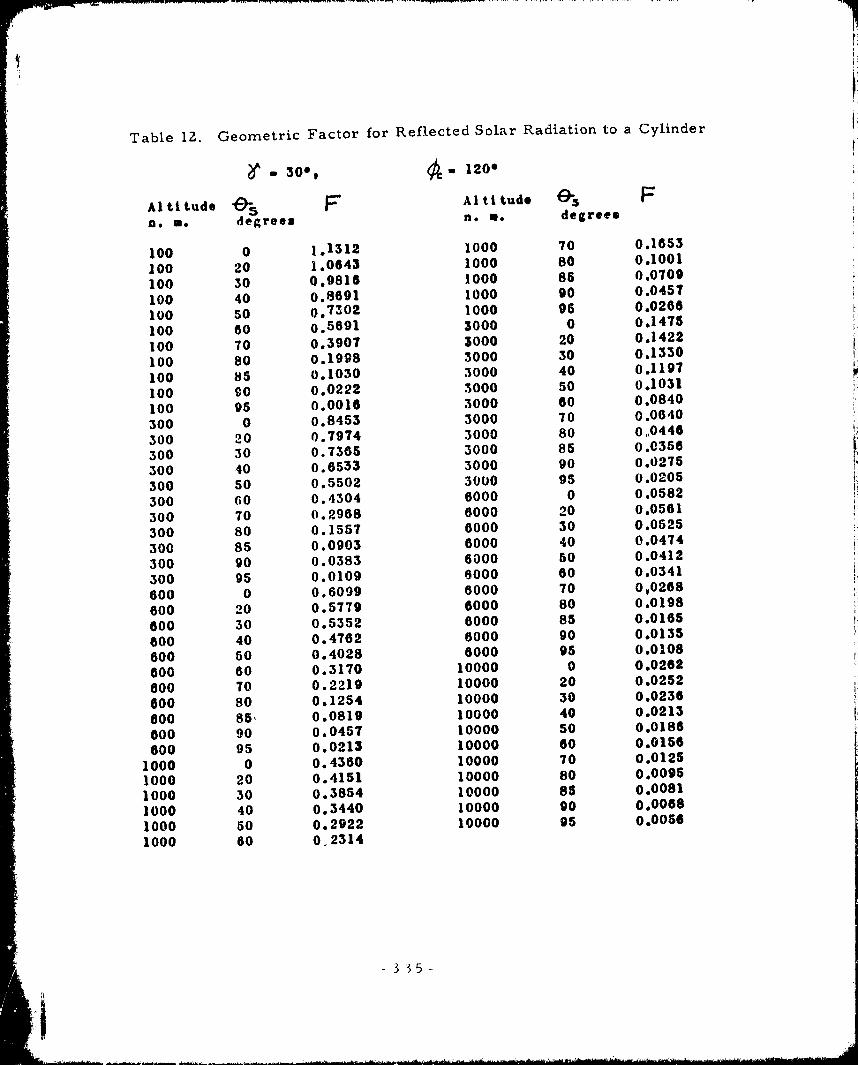
Table 12. Geometric Factor for Reflected Solar Radiation to a Cylinder

- 30, ¢. 1200

Al ti tude A F Attude 0 Fn. m. degrees n. s. degrees

100 0 1.1312 1000 70 0.1653

100 20 1.0643 1000 80 0.1001

100 30 0.9816 1000 85 0.0709

100 40 0.8691 1000 90 0.0457

100 50 0.7302 1000 96 0.0266

100 60 0.5691 3000 0 0.1475

100 70 0.3907 3000 20 0.1422

100 80 0.1998 3000 30 0.1330

100 85 0.1030 3000 40 0.1197

100 90 0.0222 3000 50 0.1031

100 95 0.0016 3000 60 0.0840

300 0 0.8453 3000 70 0.0640

300 20 0.7974 3000 80 0.0446

300 30 0.7385 3000 85 0.0356

300 40 0.6533 3000 90 0.0275

300 50 0.5502 3000 95 0.0205

300 60 0.4304 6000 0 0.0582

300 70 0.2968 6000 20 0.0561

300 80 0.1557 6000 30 0.0525

300 85 0.0903 6000 40 0.0474

300 90 0.0383 6000 50 0.0412

300 95 0.0109 6000 60 0.0341

600 0 0.6099 6000 70 0,0268

600 20 0.5779 6000 80 0.0198

600 30 0.5352 6000 85 0.0165

600 40 0.4762 6000 90 0.0135

600 50 0.4028 6000 95 0.0108

600 60 0.3170 10000 0 0.0262

600 70 0.2219 10000 20 0.0252

600 80 0.1254 10000 30 0.0236

600 85, 0.0819 10000 40 0.0213

600 90 0.0457 10000 50 0.0186

600 95 0.0213 10000 60 0.0156

1000 0 0.4360 10000 70 0.0125

1000 20 0.4151 10000 80 0.0095

1000 30 0.3854 10000 85 0.0081

1000 40 0.3440 10000 90 0.0068

1000 50 0.2922 10000 95 0.0056

1000 60 0,2314

335-

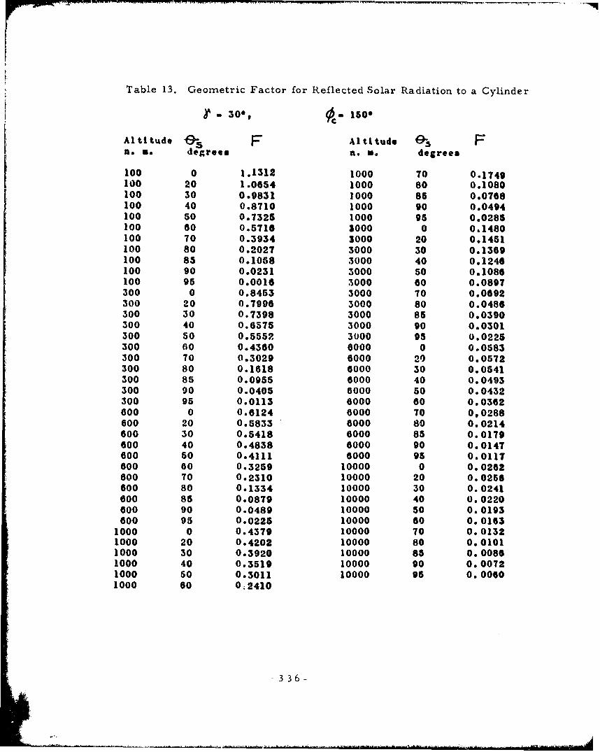
Table 13. Geometric Factor for Reflected Solar Radiation to a Cylinder

),- 30* 1500

Al ti tude F Alti.tude 0" Fn. m. degrees a. U. degrees

100 0 1.1312 1000 70 0.1749100 20 1.0654 1000 80 0.1080100 30 0.9831 1000 85 0.0768100 40 0.8710 1000 90 0.0494100 50 0.7325 1000 95 0.0285100 60 0.5716 3000 0 0.1480100 70 0.3934 3000 20 0.1451100 80 0.2027 3000 30 0.1369100 85 0.1068 3000 40 0.1248100 90 0.0231 3000 50 0.1086100 95 0.0016 5000 60 0.0897300 0 0.8453 3000 70 0.0692300 20 0.7996 3000 80 0.0486300 30 0.7398 3000 85 0.0390300 40 0.6575 3000 90 0.0301300 50 0.5552 3000 95 0.0225300 00 0.4360 6000 0 0.0583300 70 0.3029 6000 29 0.0572300 80 0.1618 6000 30 0.0541300 85 0.0955 6000 40 0.0493300 90 0.0405 6000 50 0.0432300 95 0.0113 8000 60 0.0362600 0 0.6124 6000 70 0,0288600 20 0.5833 6000 80 0.0214600 30 0.6418 6000 85 0.0179600 40 0.4838 6000 90 0.0147600 60 0.4111 6000 95 0.0117600 60 0.3259 10000 0 0.0262600 70 0.2310 10000 20 0.0256600 80 0.1334 10000 30 0.0241600 85 0.0879 10000 40 0.0220600 90 0.0489 10000 50 0.0193600 95 0.0225 10000 60 0. 0163

1000 0 0.4379 10000 70 0.01321000 20 0.4202 10000 80 0. 01011000 30 0.3920 10000 85 0. 00861000 40 0.3519 10000 90 0. 00721000 50 0.3011 10000 95 0. 00601000 60 0;2410

-3 36-

Table 14. Geometric Factor for Reflected Solar Radiation to a Cylinder

,o 30P mC 180°

Altitude F Altitude 1'- Fn. so degree* n.o . degrees

100 0 1.1312 1000 70 0.1785

100 20 1.0657 1000 80 0.1107

100 30 0.9837 1000 85 0.0787

100 40 0.8717 1000 90 0.0505

100 50 0.7333 1000 95 0.0291

100 60 0.5726 3000 0 0.1484

100 70 0.3945 5000 20 0.1462

100 80 0.2037 3000 30 0.1384100 85 o,1068 3000 40 0.1264

100 90 0.0233 3000 50 0.1106

100 95 0.0016 3000 60 0.0917300 0 0.8453 3000 70 0.0710

300 20 0.8004 3000 80 0.0499300 30 0.7410 3000 85 0.0401

300 40 0.6590 3000 90 0.0310

300 50 0.5570 3000 95 0.0231300 60 0.4381 8000 0 0.0584300 70 0.3051 6000 20 0.0576

300 80 0.1640 6000 30 0.0546

300 85 0.0972 6000 40 0.0500300 90 0.0411 6000 50 0.0440300 95 0.0114 8000 s0 0.0370600 0 0.6135 6000 70 0,0294600 20 0.5854 6000 80 0.0219

600 30 0.5443 6000 85 0.0184

600 40 0.4867 8000 90 0.0151

600 50 0.4143 6000 95 0.0121600 60 0.3292 10000 0 0.0262

600 70 0.2343 100 00.0258600 80 0.1362 10000 30 0.0243

600 85 0.0899 10000 40 0.0222

600 90 0.0499 10000 50 0.0196

600 95 0.0229 10000 60 0.0166

1000 0 0.4389 10000 70 0.01341000 20 0.4224 10000 80 0.01031000 30 0.3947 10000 85 0.00881000 40 0.3550 10000 90 0.00741000 60 0.3045 10000 95 0.00611000 80 0ý244

-337-

Table 15. Geometric Fa~ctor for Reflected Solar Radiation to a Cylinder

6'-00* 00

Altitude F Ati tude Fiin.mo. degrees n. a. degrees

100 0 1.2133 1000 70 0.1762100 20 I. 1369 1000 80 0.0912100 30 1.0460 1000 8a 0.0564100 40 0.9234 1000 90 0.0307100 50 0. 7727 1000 965 0.014100 60 0.5985 3000 0 0.2292100 70 0.4061 3000 20 0.2117100 80 0.2003 3000 30 0.1931100 85 0.0963 3000 40 0.1686100 90 0.0123 3000 50 0.1394100 95 0. 0006 3000 60 0.1076300 0 0. 9612 3000 70 0.0760300 20 0.8966 3000 80 0.0480300 30 0. 8227 3000 85 0.0362300 40 0. 7238 3000 90 0.0264300 50 0. 6029 3000 95 0.0185

S300 60 0. 4637 6000 0 0.0962300 70 0. 3097 6000 20 0.0891300 80 0. 1483 6000 30 0. 0814300 85 0. 0736 6000 40 0.0714300 90 0. 0211 6000 50 0.0599300 95 0. 0041 6000 60 0.0477600 0 0. 7441 6000 70 0,0358600 20 0. 6915 6000 80 0.0250600 30 0. 6331 6000 85 0.0203600 40 0. 5556 6000 90 0.0161600 50 0. 4610 6000 95 0.0125600 60 0. 3521 10000 0 0.0444600 70 0. 2325 10000 20 0.0412000 80 0. 1140 10000 30 0. 0378600 85 0. 0631 10000 40 0.0334600 90 0. 0274 10000 50 0.0284600 95 0. 0090 10000 60 0. 0232

1000 0 0. 5712 10000 70 0. 01801000 20 0. 5291 10000 so 0. 01321000 30 0. 4835 10000 85 0. 01111000 40 0. 4232 10000 90 0.00911000 50 0. 3500 10000 95 0. ,00741000 60 0, 2658

-338 -

Table 16. Geometric Factor for Reflected Solar Radiation to a Cylinder

i 60, 30

Al ti tud e F Al ti tude 0'3 Fn. a. degrees no M. degrees

100 0 1.2133 1000 70 0.1794

100 20 1.1373 1000 80 0.0945

100 30 1.0467 1000 85 0.0596

100 40 0.9243 1000 90 0.0335

100 50 0.7736 1000 95 0.0171

100 60 0.5996 3000 0 0.2293100 70 0.4073 3000 20 0.2123100 80 0.2015 3000 30 0.1939100 85 0.0976 3000 40 0.1490

100 90 0.0137 3000 50 0.140?

100 95 0.0009 3000 60 0.1091

300 0 0.9613 3000 70 0.0776

300 20 0.8975 3000 80 0.0494

300 30 0.8240 3000 85 0.0376

300 40 0.7255 3000 90 0.0276

300 50 0.6049 3000 95 0.0195

300 60 0.4680 6000 0 0.0982

300 70 0.3121 6000 20 0.0893

300 8o 0.1510 6000 30 0.0817

300 85 0.0764 6000 40 0.0718

300 9o 0.0237 8000 50 0.0604

300 95 0.0054 6000 so 0.0482

600 0 0.7438 6000 70 0,0363

600 20 0.6924 8000 80 0.0255

600 30 0.6346 6000 85 0.0207

600 40 0.5575 6000 90 0.0165

600 50 0.4634 6000 95 0.0128

600 60 0.3549 10000 0 0.0444

800 70 0.2356 10000 20 0.0413

600 80 0.1174 10000 30 0.0379

600 85 0.0665 10000 40 0.0336

Go0 90 0.0304 10000 50 0.0286

800 95 0.0117 10000 60 0.0233

1000 0 C.5712 10000 70 0.0188

1000 20 0.5302 10000 80 0.01341000 30 0.4851 10000 85 0.0112

1000 40 0/.253 10000 90 0.0093

1000 o0 0.3525 10000 95 0.0075

1000 06 0.2686

3 3 93 -

baaa aa

Table 17. Geometric Factor for Reflected Solar Radiation to a Cylinder

-A-,o* 60o 600

Alti tude 9& F Altttuds S. Fla. as degrees tA, me degrees

100 0 1.2133 1000 70 0.1880

100 20 1.1386 1000 80 0.10.12

100 30 1.0484 1000 85 0.0676

100 40 0.9264 1000 90 0.0406100 50 0.7763 1000 95 0.0222

100 60 0.6026 3000 0 0-2294

100 70 0.4105 3000 20 0.2139100 80 0.2049 3000 30 0.1963

100 85 0. 1012 3000 40 0.1727100 90 0.0172 3000 50 0.1443100 95 0.0013 3000 60 C.1130

300 0 0. 9613 3000 70 0.0816

* 300 20 0.9000 3000 80 0.0532300 30 0. 8276 3000 85 0.0410300 40 0. 7301 3000 90 0.0306

300 50 0.6104 3000 95 0.0221300 60 0.4722 6000 0 0.0962

300 70 0.3188 6000 20 0.0899

300 80 0.1580 6000 30 0.0826300 85 0.0830 6000 40 0.0730

300 90 0.0300 6000 50 0.0617

300 95 0.0082 6000 60 0.0496

600 0 0.7439 6000 70 0,0377

600 20 0.6955 6000 80 0.0267

600 30 0.6391 6000 85 0.0219

600 40 0.5633 6000 90 0.0176

600 50 0.4704 6000 95 0.0138

600 60 0.3628 10000 0 0.0444

600 70 0.2442 10000 20 0.0416

600 80 0.1265 10000 30 0.0383

600 85 0.0754 10000 40 0.0340600 90 0.0378 10000 50 0.0291

600 95 0.0165 10000 60 0.0238

1000 0 0.5713 10000 70 0.0187

1000 20 0.5334 10000 89 0.0138

"1000 30 0.4898 10000 85 0.0116

1000 40 0.4312 10000 90 0.0096

1000 50 0.3695 10000 95 0.0078

1000 60 0,2765

340

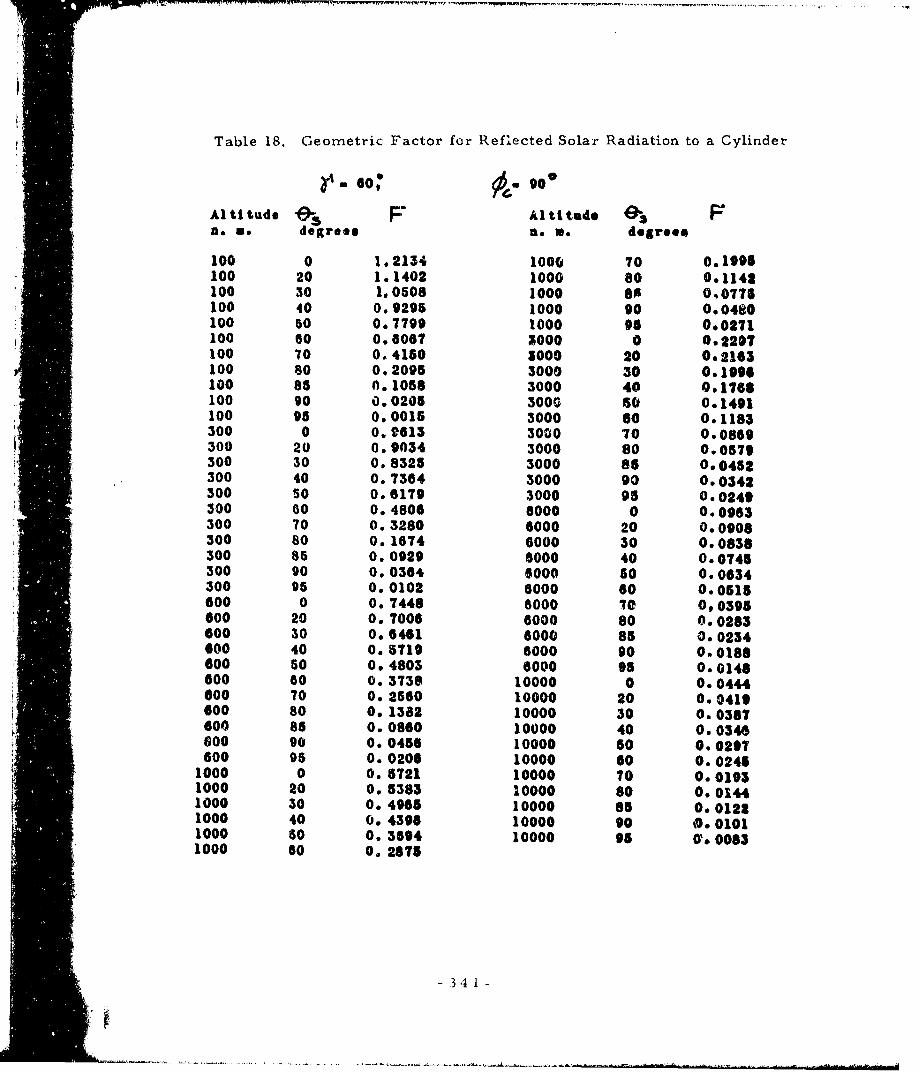
Table 18. Geometric Factor for Reflected Solar Radiation to a Cylinder

r, 60, G 900

Al tuide 1- FF Altitude e- lno o degrees e. m. degrees

100 0 1.2134 1000 70 0.1995100 20 1.1402 1000 80 0.1142lO0 30 1.0508 1000 8a 0,0775100 40 0.9295 1000 90 0.0480100 50 0.7799 1000 96 0,0271100 60 0.8067 1000 0 0.2297100 70 0.4150 3000 20 0.2163100 80 0.2095 3000 30 0.1996100 85 0.1058 3000 40 0.1766100 90 0.0205 3000 so 0.1491100 95 0.0015 3000 s0 0.1183300 0 0.9613 3000 70 0.0869300 20 0.9034 3000 80 0.0579300 30 0.8325 3000 85 0.0452300 40 0. 7384 3000 90 0.0342300 so 0.6179 3000 95 0.0249300 60 0. 4806 6000 0 0.0963300 70 0. 3280 6000 20 0.0908300 80 0.1674 6000 30 0.0838300 85 0. 0929 6000 40 0.0745300 90 0. 0364 6000 50 0.0634300 95 0. 0102 6000 60 0.0515600 0 0.7448 6000 70 0,0395600 20 0. 7006 6000 80 0.0283600 30 0.6461 6000 85 0.0234600 40 0.5719 6000 90 0.0188600 50 O. 4803 6000 95 0.0148600 @0 O. 3738 10000 0 0. 0444600 TO 0. 2560 10000 20 0. 0419600 80 0. 1382 10000 30 0. 0387o60 85 0.0860 10000 40 0.0348

600 90 O.0 456 10000 50 0.0297600 95 0. 0206 10000 60 0. 0245

1000 0 0. 5721 10000 70 0. 01931000 20 0.5383 10000 0o 0.01441000 30 0. 4965 10000 85 0. 01221000 40 0, 4398 10000 90 0. 01011000 o0 0. 3694 10000 95 0. 00831000 60 o. 2875

-341-

Table 19. Geometric Factor for Reflected Solar Radiation to a Cylinder

-80,p A: 120*

* Altitude F Al.titude 0 Fn. me degrees 13. Me degrees

100 0 1.2134 1000 70 0.2108

100 20 1.1418 1000 80 0.1237100 30 1.0532 1000 85 0.0849100 40 0.0325 1000 so 0.0529100 so 0.7835 1000 96 0.0298100 60 0.6107 3000 0 0.2300100 70 0.4194 3000 20 0.2187100 80 0.2141 3000 30 0.2030100 85 0.1102 3000 40 0.1810100 90 0.1219 3000 50 0.1539100 95 0.0015 5000 80 0.1234300 0 0.9614 3000 70 0.0917

300 20 009067 5000 80 0.0619300 30 0.8374 3000 85 0.0486300 40 0.7427 3000 90 0.0369

*300 50 0.6254 3000 95 0.0270300 60 0.4891 8000 0 0.0904300 70 0.3371 8000 20 0.0917300 80 0.1785 8000 30 0.0850

300 85 0.1005 6000 40 0.0760300 g0 0.0398 8000 50 0.0652300 95 0.0108 8000 60 0.0533

000 0 0.7470 8000 70 090412

800 20 0.7067 6000 80 0.0298

600 30 0.6539 8000 85 0.0246

000 40 0.5812 6000 90 0.0199

600 50 0.4909 8000 98 0.0158

800 80 0.3852 10000 0 0.0444

6 00 70 0.2679 10000 20 0.0422

600 80 0.1488 10000 30 0.0392

800 85 0.0942 10000 40 0.0363

000 90 0.0502 10000 50 0.0303

800 95 0.0224 10000 60 0.02521000 0 0.5736 10000 70 0.01991000 20 0.6438 10000 80 0.01417

1000 30 0.5038 10000 85 0 '1000 40 0.4484 10000 90 0.0105

1000 60 0.3794 10000 95 0.0086

1000 60 0;2985

3-3 -

•|iii

Table 20, Geometric Factor for Reflected Solar Radiation to a Cylinder

60 . 1500

Altitude F' F Altitude (-F

n.o . degrees n. .w degreeo

100 0 1.2134 1000 70 0.2187100 20 1.1430 1000 80 0.1294100 30 1.0549 1000 85 0.0888100 40 0.9347 1000 90 0.0549

100 50 0.7862 1000 95 0.0306100 60 0.6137 3000 0 0.2304100 70 0.4226 3000 20 0.2206100 80 0.2175 3000 30 0,2055100 85 0.1132 3000 40 0.1841100 90 0.0219 3000 50 0.1575100 95 0.0013 3000 60 0.1270300 0 0.9614 3000 70 0.0950300 20 0.9092 3000 80 0-0644300 30 0.8410 3000 85 0.0507300 40 0.7473 3000 90 00385300 50 0.6309 3000 95 0.0282300 60 0.4953 6000 0 0.0965300 70 0.3438 6000 20 0.0923300 80 0.1827 6000 30 0.0860300 85 0.1048 6000 40 0.0771300 90 0.0406 6000 50 0.0664300 95 0.0105 6000 60 0.0545600 0 0.7499 6000 70 0.0423600 20 0.7123 6000 80 0.0307

600 30 0.6606 6000 85 0.0254600 40 0.5888 6000 90 0,0206600 60 0.4992 6000 95 0.0163600 60 0.3940 10000 0 0,0445600 70 0.2766 10000 20 0.0424600 80 0.1555 10000 30 0.0395600 85 0.0985 10000 40 0.0355600 90 0.0518 10000 50 0.0308600 95 0.0226 10000 60 0.0256

1000 0 0.5755 13000 70 0,02031000 20 0.5485 10000 80 0.01531000 30 0.5096 10000 85 0.01301000 40 0.4553 10000 90 0.01081000 50 0.3871 10000 95 0.00891000 60 0,3061

-34 3-

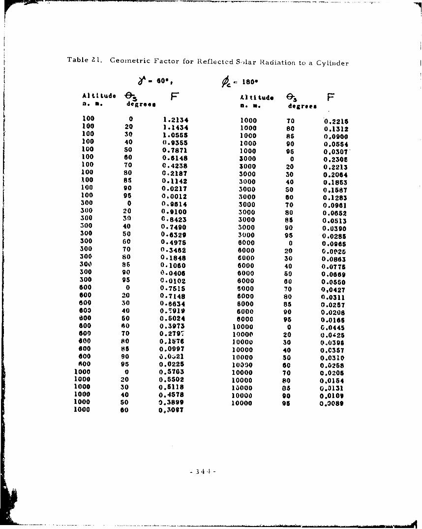
Table 1.I. Geometric Factor for Reflected S-flar Radiation to a Cylinder

' o. 60*, & 180"

Al ti tude 9; F Altitude O9 Fa. m. degrees m. s. degrees

100 0 1.2134 1000 TO 0.2215100 20 1.1434 1000 80 0.1312100 30 1.0555 1000 86 0.0900100 40 0.9355 1000 90 0.0564100 50 0.7871 1000 96 0.030?100 60 0.6148 3000 0 0.2306100 70 0.4238 3000 20 0.2213100 80 0.2187 3000 30 0.2064100 89 0.1142 3000 40 0.1853100 90 0.0217 3000 so 0.1587100 95 0.0012 3000 60 0.1283300 0 0I0614 3000 70 0.0961300 20 0.9100 3000 80 0.0652300 30 6.8423 3000 8: 0.0513300 40 0.7490 3000 90 0.0390300 50 0.6329 3000 95 0.0285300 60 0.4975 6000 0 0.0966300 70 0.3462 6000 20 0.0e26300 80 0.1848 6000 30 0.0863300 86 0.1060 6000 40 0.0775300 90 0.0406 8000 50 0.0669300 95 0.0102 6000 60 0.0550600 0 0.7515 6000 70 0,0427600 20 0.7148 6000 80 0.0311600 30 0.6634 6000 85 0.0257600 40 0.S919 6000 90 0.0208600 50 0.5024 6000 95 0.0165600 60 0.3973 10000 0 G.0445600 70 0.279K 10000 20 0.0425600 80 0.1576 10000 30 0.0396600 85 0.0997 10000 40 0.C357600 90 0.0ýo21 10000 50 0.0310600 95 0.0225 10300 60 0.0258

1000 0 0.5763 10000 70 0.02051000 20 0.5502 10000 80 0.01541000 30 0.5118 10000 05 0.31311000 40 0.4578 10000 90 0.01091000 s0 0.3899 10000 95 0.00891000 60 0.302?

-344-

Table 2Z. Geometric Factor for Reflected Solar Radiation to a Cylinder

g* 90". -0'

Altitude F Al ti tudo Fn. m. degrees no. n. degrees

100 0 1.2702 1000 70 0.2216100 20 1.1936 1000 80 0.1238100 30 1.1000 1000 86 0.0813100 40 0.9730 1000 90 0.0478100 50 0.8164 1000 96 0.0252100 60 0.6351 3000 0 0.2820100 70 0.4344 3000 20 0.2467100 80 0.2193 3000 30 0.2277100 85 0.1099 3000 40 0.2016100 90 0.0164 3000 50 0.1699100 95 0.0007 3000 60 0.1345300 0 1.0357 3000 70 0.0982300 20 0.9733 3000 80 0.0645300 30 0.8970 3000 85 0.0499300 40 0.7934 3000 90 0.0473300 50 0.66857 3000 95 002683300 60 0.5178 6000 0 0.1107300 70 0,3534 6000 20 0.1043300 80 0.1793 8000 30 0.0963300 85 0.0960 6000 40 0.0856300 90 0.0320 8000 50 0.0728300 95 0.0070 8000 60 0.0590600 0 0.8221 8000 70 0,0451600 20 0.7731 6000 80 0.0322600 30 0.7127 6000 85 0.0264600 40 0.6308 6000 90 0.0212600 50 0.5296 6000 95 0.0167600 60 0.4120 10000 0 0.0512600 70 0.2815 10000 20 0.0482600 80 0.1490 10000 30 0.0446600 85 0.0890 10000 40 0.0398600 90 0.0431 10000 50 0.0342600 95 0.0172 10000 60 0.0282

1000 0 0.6394 10000 70 0.02221000 20 0.6015 10000 80 0.01661000 30 0.5546 10000 85 0.01391000 40 0.4910 10000 90 0.01161000 50 0.4124 10000 95 0.00941000 60 0,3207

-345-

Table 23, Geonmetri.c Factor for Reflected Solar Radiation to a Cylinder

go*, 90o A- 30'

Alt tude e- Al titude F"i i. m. degrees n.o . degreto

100 0 1.2702 1000 70 0.2217

100 20 1.1936 1000 80 0.1245

100 30 1.1000 1000 86 0.0823

100 40 0.9730 1000 90 0.0489

300 60 0.8164 1000 95 9.0262

100 60 0.8351 3000 0 0.2019

100 70 0.4344 3000 20 0.2466

100 80 0.2193 3000 30 0.2276

100 85 0.1101 3000 40 0.2016

100 90 0.0174 3000 50 0.1899

100 95 0.0009 3000 80 0.1346

300 0 1.0357 3000 70 0.0983

300 20 0.973M 3000 80 0.0648

300 30 0.8070 3000 86 0.0502

"300 40 0.7934 3000 90 0.0376

300 50 0.6e57 3000 v5 0.0201

300 00 0.5178 6000 0 0.1107

300 70 0.3534 6000 ?o 0.1043

300 80 0.1705 6000 30 0.0963

300 85 0.0969 6000 40 0.0855

300 90 0.0334 6000 r0 0.0728

300 95 0.007j 6000 30 0.C590

800 0 0.8209 6000 70 0,0451

600 20 0.7721 6001 80 0.01.W

600 30 0O J119 0000 85 0.0265

G600 40 6.6300 6600 90 0. 0213

600 5C 0. 5291 6000 95 0.017

600 80 0.4116 10000 0 010512

000 7 O. 2814 10000 24 0.0482

600 80 0. 1496 10000 s0 0.0446

600 05 0. Ot101 10000 40 0.0398

600 90 0. 0444 10000 50 0.0342

601 95 O. G183 10000 60 0.0281

1000 0 0. 6387 10000 70 0.0222

l000 20 o.6009 10000 80 0.016O

1000 50 0. 5542 10000 85 0.0139

1003 40 0. 4906 1O0000 90 0.0116

1000 50 0. 4121 10000 95 0. 0094

1000 60 0, 3205

3 i4

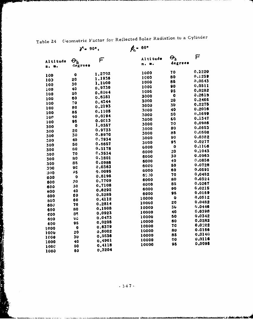
Table 24 G;eometric Factor foi Reflected Solar Radiation to a Cylinder

?a. 90, G 6o

AliAd I~ Flti tude 93Fn. *. ,legreeS n.*. degree

100 0 1.2702 1000 70 0.2220

103 20 1.1936 1CO0 80 0.1259

100 30 1.1000 1000 86 0.0643

l00 40 0.9730 1000 90 0.0511

100 50 0.8164 1000 95 0,0282

100 60 0.6351 3000 0 0.2618

"100 00 0.4344 3000 20 0.2405100 80 0.2193 3000 30 0.2275100 80 0.1105 3000 40 0.2016

10o 90 0.0194 3000 50 0.1699

100 95 0.0013 3000 60 0.1347

300 0 1.0357 3000 70 0.0986

300 20 0.9733 3000 80 0.0653

300 30 0.8970 3000 86 0.0508

100 40 0.7934 3000 90 0.0382

300 50 0.6657 3000 95 0.0217

300 00 0.5178 0000 0 O.I]G6

300 70 0.3534 6000 20 0.1043

300 80 0.1801 6000 30 0.0963

300 85 0.0986 6000 40 0.0856

300 90 0.0383 6000 50 0.0728

300 45 010095 6000 60 0.0591

G00 0 0.8196 6830 70 0,0452

600 20 0.7709 6000 80 0.0324

600 30 0.7108 6000 85 0.0267

100 40 0.6292 6000 90 0.0215

600 g0 0.5285 6000 95 0.0169

600 60 0.4112 10000 0 0.0512

600 70 0.2814 10000 20 0.0482

600 80 0.1508 10000 30 0.0446

0OO 3i 0.0923 10000 40 0.0398

600 Vz 0.0473 10000 50 0.0342

600 95 0.0205 10000 60 0.0282

1000 0 0.6379 10000 70 0.0222

1000 20 0.6002 10000 80 0.0166

1000 30 0.5536 10000 85 0.0140

1000 40 0.4901 10000 s0 0.0116

1000 50 0.4118 10000 95 0.0095

1000 60 0.3204

-347-

,4

Table 25. Geometric Factor for Aeflected Solar Radiation to a Cylinder

go* or.- 901

Altitude F Al ti tud. f9 Fn. m. dearees no. degrees

100 0 1.2702 1000 70 0.2222100 20 1.1936 1000 80 0.1266100 30 1.1000 1000 85 0.0853100 40 0.9730 1000 90 0.0523100 50 0.8164 1000 95 0.0292100 i0 0.6351 3000 0 0.2607100 70 0.4344 3000 20 0.2465100 80 0.2193 3000 30 0.2275100 85 0.1107 3000 40 0.20150oo 90 0.0206 3000 50 0.1699

100 95 0.0015 3000 60 0.1347300 0 1.0358 3cCO 70 0.0988300 20 0.9733 3000 80 0.0656300 30 0.8970 3000 as 0.0512300 40 0.7934 3000 90 0.0Z86

o00 50 0.6657 3000 95 0.0281300 00 0.5178 6000 0 0.1106300 70 0.3534 0000 20 0.1043300 so 0.1803 6000 30 0.0963300 85 0.0994 6000 40 0.0856300 90 0.0379 6000 50 0.0729300 95 0.0104 6000 60 0.0591600 0 0.8192 6000 70 090453800 20 0.7703 6000 80 0.0325600 30 0.7106 6000 85 0.0267000 40 0.0290 6000 90 0.0215S00 60 0.5283 6000 95 0.0170600 s0 0.4111 10000 0 0.0512COO TO 0.2814 10000 20 0.0482600 80 0.1514 10000 30 0.0446600 85 0.0934 10000 40 0.03986W0' 90 0.0487 10000 50 0.0342400 95 0.0219 10000 60 0.02821000 0 0.6377 10000 70 0.02221000 20 0.6001 10000 80 0.01661000 30 0.5535 10000 85 0.0140100 40 0.4900 10000 D0 0.01U61000 b0 0.4117 10000 95 0.00951000 60 003204

-348-

Table 26. Geometric Factor for Reflected Solar Radiation to a Cylinder

It 90g, 04, 1200

Al ti tude ' F Al ti tude Q. Fn.o . degrees ne . degrees

100 0 1.2702 1000 70 0.2220

100 20 1.1936 1000 80 0.1259

100 30 1.1000 1000 86 0.0843

100 40 0.9730 1000 90 0.0511

100 50 0.8164 1000 96 0.0282

100 60 0.6351 3000 0 0.2618

100 70 0.4344 3000 20 0.2466

100 80 0.2193 3000 30 0.2276

100 85 0.1105 3000 40 0.2016

100 90 0.0194 3000 50 0.1699

100 95 0.0013 3000 60 0.1347

300 0 1.0357 3000 70 0.0987

300 20 0.9733 3000 80 0.0654

300 30 0.8970 3000 86 0.0508

300 40 0.7934 3000 90 0.0382

300 50 0.6657 3000 95 0.0277

300 00 0.5178 6000 0 0.1106

300 70 0.3534 6000 20 0.1043

300 80 0.1801 8000 30 0.0963

300 85 0.0986 6000 40 0.0856

300 90 0.0363 6000 50 0.0728

300 95 0.0095 6000 G0 0.0591

600 0 0.8201 8000 70 0,0452

600 20 0.7714 6000 80 0.0324

600 30 0.7113 6000 85 0.0267

600 40 0.6296 6000 90 0.0215

600 60 0.6287 6000 95 0.0169

600 60 0.4114 10000 0 0.0512

600 70 0.2815 10000 20 0.0482

600 80 0.1508 10000 30 0.0446

600 85 0.0923 10000 40 0.0398

600 90 0.0473 10000 50 0.0342

600 95 0.0205 10000 60 0.0282

1000 0 0.6383 10000 70 0.0222

1000 20 0.6005 10000 80 0.0166

1000 30 0.5538 10000 85 0.0140

1000 40 0.4903 10000 90 0.0116

1000 60 0.4119 10000 96 0.00951000 60 0,3205

349-

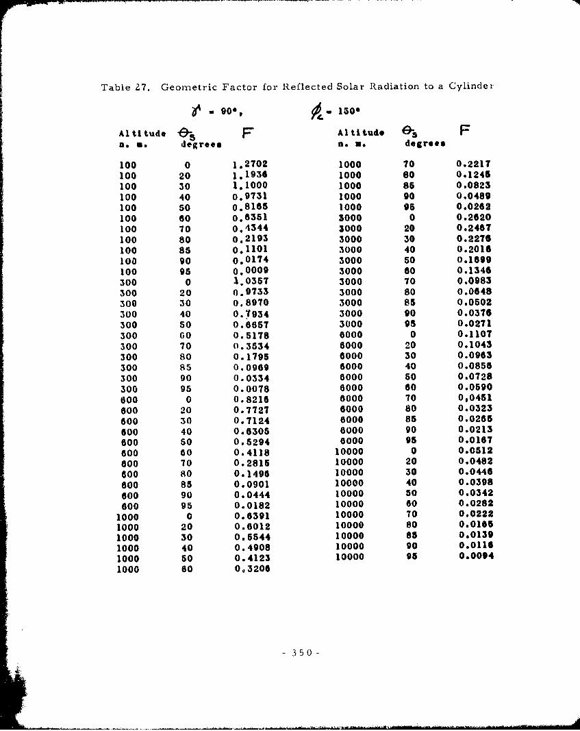
Table 27. Geometric Factor for Reflected Solar Radiation to a Cylinder

go*,A 130*

Al ti tude F Altitude Fno a. degree. no so degree.

100 0 1.2702 1000 70 0.2217100 20 1.1936 1000 80 0.1245100 30 1.1000 1000 86 0.0823100 40 0.9731 1000 90 0.0489100 50 0.8165 1000 95 0.0262100 60 0.6351 3000 0 0.2620100 70 0.4344 3000 20 0.2467100 80 0.2193 3000 30 0.2276100 86 0.1101 3000 40 0.2016100 90 0.0174 3000 50 0.1699100 95 0.0009 3000 60 0.1346300 0 1.0357 3000 70 0.0983300 20 0.9733 3000 80 0.0648

300 30 0.8970 3000 85 0.0502

300 40 0.7934 3000 90 0.0376

300 50 0.8657 3000 95 0.0271

300 GO 0.5178 6000 0 0.1107300 70 0.3534 6000 20 0.1043

300 80 0.1795 6000 30 0.0963

300 85 0.0969 6000 40 0.0856

300 90 0.0334 6000 50 0.0728300 95 0.0078 6000 60 0.0690

600 0 0.8216 6000 70 0,0451

600 20 0.7727 6000 80 0.0323

600 30 0.7124 6000 85 0.0265

600 40 0.6305 6000 90 0.0213

600 50 0.5294 6000 95 0.0167

600 60 0.4118 10000 0 0.0512

600 70 0.2815 10000 20 0.0482

600 80 0.1496 10000 30 0.0446

600 85 0.0901 10000 40 0.0398

600 90 0.0444 10000 50 0.0342

600 95 0.0182 10000 60 0.0282

1000 0 0.6391 10000 70 0.0222

1000 20 0.6012 10000 80 0.01685

1000 30 0.6544 10000 85 0.0139

1000 40 0.4908 10000 90 0.0116

1000 50 0.4123 10000 95 0.0094

1000 60 0,3206

-350-

. . .

TabLe 28. Geometric Factor for Reflected Solar Radiation to a Cylinder

- 90", 1800

Altti tude F AItitude 93 Fn. m. degrees a. we degrees

100 0 1.2702 1000 70 0,2216100 20 1.1936 1000 80 0.1238100 30 1.1000 1000 86 0.0813100 40 0.9730 1000 90 0.0478100 50 0.8164 1000 96 0.0252100 60 0.6351 3000 0 0.2620100 70 0.4344 3000 20 0.2467100 80 0.2193 3000 30 0.2277100 85 0.1099 3000 40 0.2016100 90 0.0164 3000 50 0.1699100 95 0.0007 3000 60 0.1345300 0 1.0357 3000 70 0.0982300 20 0.9733 3000 80 0.0845300 30 0.8970 3000 85 0.0499300 40 0. 7934 3000 90 0.0373300 50 0.6657 3000 95 0.0288300 60 0.5178 8000 0 0.1107300 70 0.3534 6000 20 0.1043300 80 0.1793 6000 30 0.0963300 85 0.0960 6000 40 0.0856300 90 0.0320 6000 s0 0.0728300 98 0.0070 8000 80 0.0590600 0 0.8221 6000 70 0,0451800 20 0.7731 6000 80 0.0322600 30 0.7127 6000 85 0.0264G00 40 0.6308 6000 90 0.0212600 50 0.5296 6000 95 0.0167600 80 0-4120 10000 0 0.0512800 70 0.2815 10000 20 0.0482600 80 0.1490 10000 30 0.0446600 85 0.0890 10000 40 0.0398600 90 0.0431 10000 50 0.0342600 95 0.0172 10000 60 0.0282

1000 0 0.8394 10000 70 0.02221000 20 0.5546 10000 80 0,018$1000 30 0.6015 10000 85 0.01391000 40 0.4910 10000 g0 0.01161000 50 0.4124 10000 95 0.00941000 60 0a3207

-351-

Figure 7. Geometry for Planetary Reflected Solar Radiation to a Hemitpherc

Geometric Factor, F q

'HEMISP)HERE

SUN

-TE R.MINATOR

-352-

A• ...

, Table 29. Geometric Factor for R<eflected Solar Radiation to a Hemisphere

i i o. ,,. k -360o

Al titude e'- F A l titude • F'r *. degrees no as dogrees

100 0 1.2438 1000 70 0.2211

100 20 1.1688 1000 so 0.1247

100 30 1.0771 1000 85 0.0829

100 40 0.9528 1000 90 0.0497

100 50 0.7995 1000 95 0.0210

100 60 0.6219 3000 0 0.261?

100 70 0,4254 5000 20 0.2465

100 80 0.2147 3000 30 0.2275

100 85 0.1079 3000 40 0.2015

100 90 0.0177 3000 s0 0.1698

100 95 nl.0010 3000 60 0.1345

300 0 1.0231 3000 70 0.0984

300 20 0.9620 3000 so 0.0650

300 30 0.8886 3000 85 0.0505

300 40 0.7842 3000 90 0.0379

300 50 0.6580 3000 95 0.0274

300 60 0.5118 8000 0 0.1106

300 70 0.3493 6000 20 0.1043

300 80 0.1777 8000 30 o.o9b3

300 85 0.0984 6000 40 0.0855

300 90 0.0342 6000 50 0.0728

"300 95 0.0084 8000 60 0.0590

600 0 0.8154 6000 70 0,0452

600 20 0.7669 6000 so 0.0323

600 30 0o7071 6000 85 0.0266

600 40 0.6259 6000 90 0.0214

800 60 0.5256 6000 95 0.0168

600 60 0.4089 10000 0 0.0512

0oo 70 0.2796 10000 20 0.0482

800 80 0.1492 10000 30 0.0446

800 8, 0.0905 10000 40 0.0398

800 90 0.0454 10000 s0 0.0342

800 95 0.0191 10000 80 0.0282

1000 0 0.6363 10000 70 0.0222

1000 20 0.5987 10000 80 0.0365

1000 30 0.5521 10000 85 0.0140

1000 40 0.4888 10000 90 0.0116

1000 50 0.4106 10000 96 0.0094

1000 60 0,3194

-353-

Table 30, Georretric Factor for Reflected Solar fRadiatiorA to a lierisphere

Al titude F AlIt itude 04a. m. degrees n. m. degrees

100 0 1. 1799 1000 70 0.2205100 20 1. 1115 1000 so 0.1286100 30 L 0259 1000 85 0.0875

100 40 0. 9091 1000 90 0.0638100 60 0. 7646 1000 95 0,0299100 60 0.5969 3000 0 0.2452100 70 0.4111 3000 20 0.2331100 80 0,2116 3000 30 0.2163100 85 0.1100 3000 40 0.1928100 90 0.0210 3000 50 0.1639100 95 0.0013 3000 60 0.1313300 0 0.9673 3000 70 0.0973300 20 0.9135 3000 80 0.0654300 30 0.8443 3000 85 0.0512300 40 0.7495 3000 90 0.0387300 5o 0.6319 3000 95 0.02S3

300 60 0.4951 6000 0 0.1034300 70 0.3424 6000 20 0.0983300 80 0.1802 o000 30 0.0912300 85 0.1021 6000 40 0.0815300 90 0.0391 8000 50 0.0698300 Z5 0.0102 6000 60 0.0570o00 0 0.7899 6000 70 090440

500 20 0.7.90 6000 80 0.0317600 30 0.6749 6000 85 0.0262600 40 0.6002 6000 90 0.0212600 50 0.5073 8U00 95 0.0!67800o 0 0 .3 986 10000 0 0.0478600 70 0.2715 10000 20 0.0464800 80 0.1537 10000 30 0.0421600 85 0.0963 10000 40 0.0377o00 90 0.0503 10000 50 0.0326600 95 0.0220 10000 60 0.0270

1000 0 0.5991 10000 70 0.02131000 20 0.5583 10000 80 0o01601000 30 0.5266 10000 85 0.01351000 40 0.4690 10000 90 0.01131000 50 0.3970 10000 95 0.00921000 60 0,3125

- 3;|1

_ -- -• •t t ~ .S t4& ,.2

Table 31. Geometric Factor for Reflected Solar Radiation to a Hemisphere

:So0ot 30

Al titude 19-S F Al ti tude 0 3 Fo o.r. degrees n. w. degrees

100 0 1.1799 1000 70 0.2188100 20 1.1112 1000 80 0.1270100 30 1.0253 1000 85 0.0862100 40 0.9084 1000 90 0.0529100 50 0.7638 1000 95 0.0293100 60 0.5960 3000 0 0.2451100 70 0.4101 3000 20 0.2327100 80 0.2105 3000 30 0.2158100 85 0.1090 3000 40 0.1923100 90 0.0204 3000 so 0.1632100 95 0.0013 3000 60 0.1305300 0 0.9873 3000 70 0.0964300 20 0.9129 3000 80 0.0648300 30 0.8434 3000 85 0.0507300 40 0.7484 3000 90 0.0383300 50 0.6305 3000 95 0.0279300 60 0.4936 6000 0 0.1034300 70 0.3407 6000 20 0.0982300 80 0.1786 6000 30 0.0910300 85 0.1006 6000 40 0.0812300 90 0.0382 6000 50 0.0896300 95 0.0099 6000 60 0.0567600 0 0.7695 6000 70 0,0437600 20 0.7280 6000 80 0.0315600 30 0.6736 6000 85 0.0260600 40 0.5987 6000 90 0.0210600 50 0.5056 6000 95 0.0166600 0.3968 0000 0 0.0478600 70 0.2756 10000 20 0.0453600 80 0.1519 10000 30 0.0420co0 85 0.0948 10000 40 0.0377000 90 0.0493 10000 50 0.0325600 95 0.0215 10000 60 0.0269

1000 0 0,5989 10000 70 0.02131000 20 0.5675 10000 80 0.01591000 30 0.5255 10000 85 0.01351000 40 0.4676 10000 90 0.01121000 50 0.3955 10000 95 0.00921000 60 0.3108

-355-

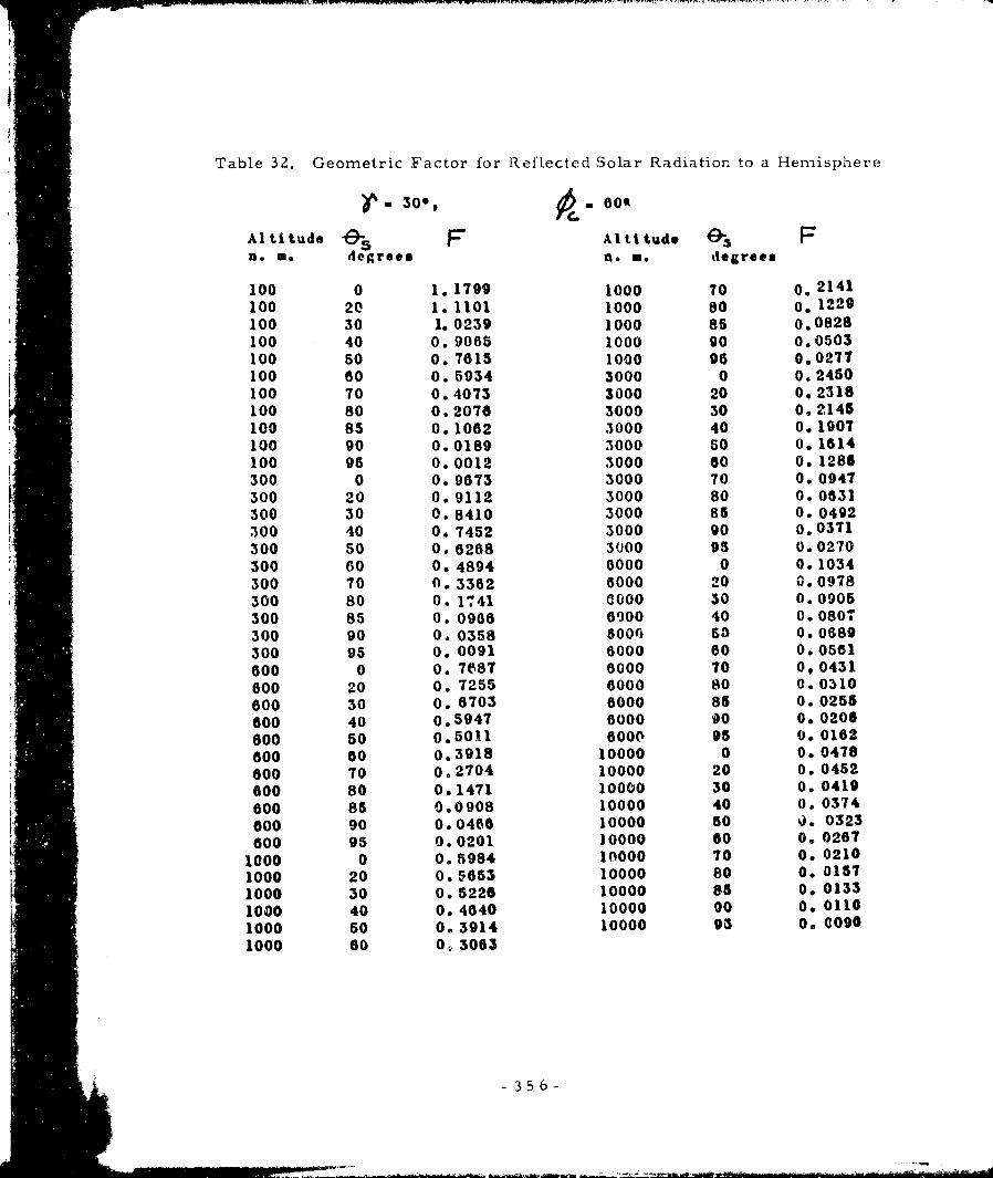
Table 32. Geometric Factor for Reflected Solar Radiation to a Hemisphere

-300, 65.01t

Al ti-tude F Altitude F.Is degrees Iken degrees

100 0 1. 1799 1000 70 0. 2141100 20 1. 1101 1000 80 0. 1229100 30 1.0239 1000 86 0:0828100 40 0. 9065 1000 90 o.0503100 50 0. 7815 1000 95 0.0277100 80 0. 5934 3000 0 0.2450100 70 0.4073 3000 20 0.2318100 80 0.2076 3000 30 0.2145100 85 0. 1082 3000 40 0.1907100 90 0. 0189 3000 s0 0. 1614100 96 0.0012 3000 60 0. 1286300 0 0. 9873 3000 70 0. 0947300 20 0. 9112 3000 80 0. 0631300 30 0. 8410 3000 85 0. 04925300 40 0. 7452 3000 90 0.0371300 50 0. 6288 3000 95 0.0270300 60 0. 4894 8000 0 0.1034300 70 0. 3382 6000 20 0.0978300 80 0. 1741 0000 30 0. 0905300 85 0. 0966 60100 40 0.080'a300 90 0. 0358 8006 5 0.0889300 95 0. 0091 8000 80 0. 0561

800 0 0. 7M7 8000 70 0, 0431600 20 0. 7255 8000 80 0. 0310600 30 0. 6703 8000 85 0. 0255600 40 o.5947 6000 00 0.0206

600 50 0.5011 6000 95 0P.0162600 60 0.3918 10000 0 0. 0478600 T0 0.2704 10000 20 0. 0452

600 80 0.1471 10000 30 0. 0419

800 85 0.0901 10000 40 0. 0374

800 90 0.0466 10000 50 o. 0323

600 95 0.0201 10000 60 0. 0267

1000 0 0. 5984 10000 70 0. 0210

1000 20 0.5853 10000 0 0. 01571000 30 0. 5226 10000 50 0. 0133

1030 40 0. 4640 10000 00 0. 0110

1000 50 0. 3914 10000 98 0. c09g

1000 60 O. 3063

0356

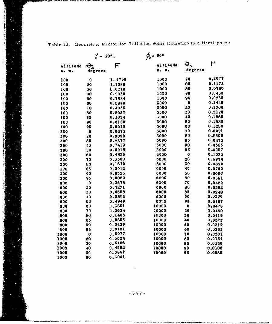
Table 33. Geometric Factor for Reflected Solar Radiation. to a Hemisphere

6 30". o.-90

Al ti tude F Al titude o- Fa. m. degrees no. . degrees

100 0 1.1799 1000 70 0.2077

100 20 1.1088 1000 80 0.1172

100 30 1.0218 1000 85 0.0780100 40 0.9039 1000 90 0.0458

100 50 0.7584 1000 95 0.0255100 60 0.5899 3000 0 0.2448100 70 0.4035 3000 20 0.2306100 80 0.2037 3000 30 0.2128100 95 0.1024 3000 40 0.1885100 90 0.0169 3000 50 0.1589100 95 0.0010 3000 60 0.1259300 0 0.9673 3000 70 0.0921300 20 0.9090 3000 80 0.0609300 30 0.8377 3000 85 0.0473

300 40 0.7410 3000 90 0.0855

300 850 0.0212 8000 40 0.0279300 60 0.4836 6000 0 0.1038300 70 0.3300 6000 20 0.0974600 80 0.1679 6000 30 0.0899300 85 0.0912 6000 40 0.0799300 90 0.0325 6000 50 0.0680300 94 0.0080 6000 60 0.0551600 0 0.7678 6000 70 090422"600 20 0.7231 6000 80 0.0302600 30 0.06658 6000 85 0.0248600 40 0.5893 6000 90 0.0200600 50 0.4949 10000 45 0.01571000 0 0.3751 10000 0 0.0478

1600 70 0.2634 10000 20 0.04500600 80 0.1406 10000 30 0.0416

••600 85 0.0953 10000 40 0.0372

1000 2o0 o.52 10000 80 0o01541000 30 o.5186 10000 ss 0101301000 40 0.4592 10000 90 0.01081000 50 o.3857 10000 95 0o00881000 80 o,3001

"-357-

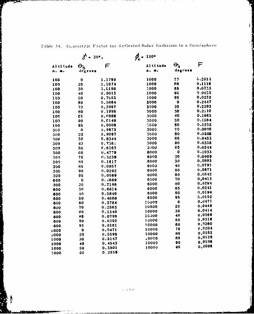
Aw-I

Table 34. (Gometric Factor tot Reflected Solar Radiation to a Heemisphere

6- 30", A- 120"

Alti tude FAl titude F I3n. a* diegrao a. U. dogroee

100 0 1.1799 1000 T• t 2014

100 20 1.1074 1000 80 0.1116t00 30 1.G198 1000 85 0.0713100 40 0.9013 1000 90 00433103 50 0.7U53 1000 95 0.0232

100 60 0.5804 3000 0 0.2447100 73 0.3997 3000 20 0.2293100 80 01998 3000 30 0.2110

ion Cý 0.0986 3000 40 0.1863

100 90 0.e149 3000 50 0,1564

100 96 0.0008 o00oo 60 0.1232

3?0 0 0.9673 3000 70 0.0895

300 20 0.9007 3000 80 0.0586300 30 0.8344 3000 85 0.0453

300 40 0.736C 3000 90 0.0338

30q 50 0.6167 3000 95 0.0244300 60 0.4779 6000 0 0.1033

309 70 0.3239 6000 20 0.0969

30') SO 0.1617 6000 30 0.0893

300 85 0.0857 6009) 40 0.0791

300 90 0.0292 6000 50 0.0671

300 95 0.0069 6000 60 0.0542

G00 0 0.1669 6000 70 0,0413

300 20 0.7188 6000 80 0.0214

600 30 0.6814 6000 85 0.0241

600 40 0.5840 6000 90 9.0194

600 50 0.4888 6000 95 C.0152

600 80 0.3784 1•000 0 0.0471

600 70 0.2563 10000 20 0.0449

000 80 0.1340 10000 30 0.0414

600 85 0.0798 1G000 40 0.0369

000 90 0.0392 )0000 50 0.0316

800 95 0.0161 0Oooo 60 0.0260

10C0 0 0.571 10000 o0 0.0204

iOoo 20 0.5595 10000 so 0.0152

1000 30 0.5147 ,0000 85 0.0128

1000 40 0.4543 10000 90 0.0106

1000 50 0.3801 10000 98 0.0086

!000 30 0.2939

Table 35. Geometric Factor for Reflected Solar Radiation to a

300 - 1500

Al ti tude e-F Al ti tude sa. M. degrees n. a. degroiea

100 0 1.1790 1000 7C 1.1987100 20 1.1064 1000 80 0.1074100 30 1.0183 1C0c 85 O.0698100 40 0.8994 1000 90 0.0408100 50 0.7531 IOOG 95 0.0216100 60 0.5839 3000 k 0.2446100 70 0.3969 3000 20 0.2284100 80 0.1969 3000 30 0.2098IGO 83 0.0958 3000 40 0.1847100 90 0.0134 3000 50 0,1545100 95 0.0007 3000 60 0.1212300 0 0.9673 3000 70 0.0876300 20 0.9050 3000 8t 0.0570300 30 0.8320 3000 8 0.0439300 40 0.7336 3000 90 u.0326300 50 0.8130 3000 95 0.C234300 60 0.4737 6000 0 0.1033300 70 0.3193 6000 20 0.0986300 80 0.1572 8000 30 0.0886300 86 0.0818 6000 40 0.0786300 g0 0.0268 6000 50 0,0665300 95 0.0061 6000C 30 0.0535600 0 0.7663 60001 TO 0,040?600 20 0.7164 6000 80 0.0289600 30 0.6582 6000 85 0.0236600 40 0.5801 6000 to0 0.018f600 50 0.4843 6000 95 0.014a600 60 0.3735 10000 0 0.047?600 7O 0.2511 10000 20 0.0447600 80 0.1292 10000 30 0.0412600 85 0.0758 1Ou5r 40 0.0367000 90 0.0365 i000M 10 040314600 95 n.0147 100(jO 60 0.0258

1000 0 0.5967 10000 70 0 A)2021000 20 0.5574 1000 40 0.01601000 30 0.5119 10000 05 0.01261000 40 0.4508 10000 00 0.01041000 50 0.3761 1 000 95 0.00851000 60 0,2894

-Taible 36. (,'licontric Factor for ]*c'fleicted Solar Radiation to a I-'emisphiere

S30, - 180*

Alti,,,d - F AltAl de ti-, F1. 6 . degree@ n. Ne. degrees

100 0 1.1709 1000 70 0,1950* . 100 20 1.1060 1000 80 0.1059

100 30 1.0178 1000 8s0568100 40 0.8.87 1ooo go 0.0399100 so 0.7522 1000 95 0.02100o0 60 o.5829 3000 0 0.2445

100 70 0.6319 3000 20 0.2281G00 80 0.1958 3000 30 0.2093

P.100 85 U,0948 3000 40 0.18-:42100 90 0.0129 3000 20 0.1039loc 95 000006 3000 60 0.1O20b

0 0 0.9073 3000 70 0.0864300 20 0.9044 3000 80 0.0684

300 0 0.8311 3000 50 0.0433NO0 40 ,.7326 U000 9o 0.0322300 o 0 0.116 3000 95 0.0231

* 300 60 0o4722 6000 0 0.1033300 70 0.3177 6000 20 o.0965300 80 C.156 10000 30 G.087'300 85 0.0803 l000 40 0.0783300 90 0.0259 6000 60 0,0e63"300 95 0.0075d 00G0 80 0.0533600 0 0.70355 8000 TO 0.0v446 800 20 0.7145 6000 80 0.028*,00 30 0.6572 8000 85 0.0234000 40 0.5787 6000 90 0.0188800 s0 0.4827 8000 95 0-0147800 60 0.3717 10000 0 0,0471

600 70 0.2493 10000 20 0.0447000 g0 0.1275 10000 30 0.0412

800 85 0.0744 10000 40 0.01366800 90 0.0355 10000 51ý 0.0313600 95 0.0142 10000 60 0.0257

1000 0 1.5963 10000 70 0.02011000 20 0.5687 10000 80 0.01401000 30 0.5109 10000 85 0.01251000 40 0.4496 10000 90 0.01041000 50 0.3746 14000 95 0.0084

1000 60 0;2871

I3n0I1 i~l! - _•6o-"1ll

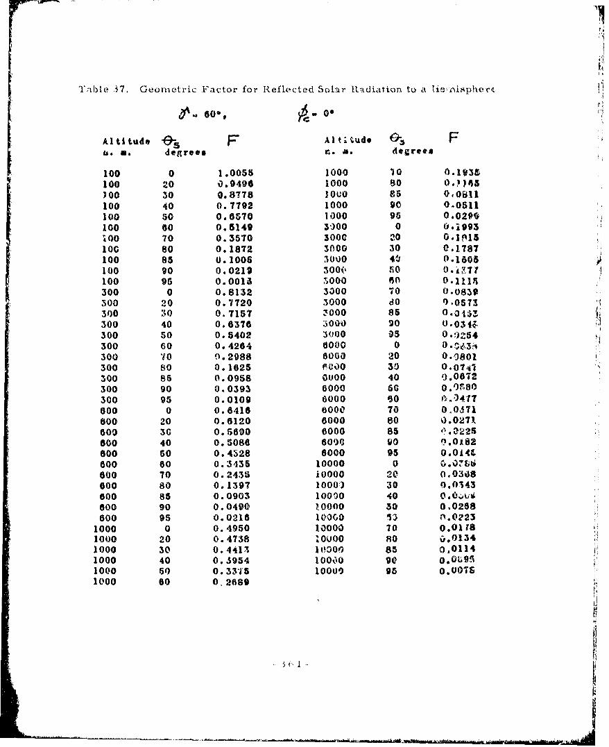
Si',bl- 37. Geounetric Factor for Reflected Solar Rladiation to a ie-i,•isphle.rf

gtu 60", - O

Al titude A.S F" AIt FIs. *. degrees n.o . degrees

100 0 1.0055 1000 10 0.193S100 20 %)9496 1000 80 00146

00 30 0.8778 1000 86 0,0811100 40 0.7792 1000 90 040511100 50 0.6570 1000 95 0.02P6100 60 0.5149 3-300 0 6.1993i00 70 0.3570 300C 20 0.1015100 80 0.1872 3000 30 0.1787100 85 0.1006 3000 40 0.1805100 90 0.0219 300( 50 0."7100 95 0.0015 5000 60 0.11 I300 0 0.8132 3300 70 0.0830300 20 0.7720 3000 do 0,0573

300 30 0.7157 ý000 85 0.0153300 40 0.6376 3000 20 0.034.300 50 0.6402 3000 05 0. 9254300 60 0.4264 6000 0 0.U31300 70 0.2988 6000 20 0.0801300 80 0.1625 600 30 0.0741300 85 0.0958 0000 40 9.06i2

300 90 0.0393 6000 56 0.0•80

300 95 0.0109 6000 60 A.147600 0 0.8416 8000 70 0,0M71800 20 0.6120 6000 80 0.027k600 30 0.5600 6000 85 ".222600 40 0.5086 6000 90 0.0i82600 60 0.4528 8000 95 0.0i4t600 60 0.3435 10000 0 G d800 70 0.2435 iOO 20 0.0348600 80 0.1397 1000) 30 0.0343600 85 0.0903 10000 40 O.bbX600 90 0.0490 ,0000 30 0,0208600 95 0.0216 10000 13 -. 0223

1000 0 0.4950 10000 70 0.01181000 20 0.4738 I0U00 so ;. 0 1 3 4

1000 30 0.4413 10000 85 0,0114 H1000 40 0.3954 100lO go o.Og•951000 60 0.3315 10000 95 0.00761000 60 0,2689

L r

ITable 38, Sconetric Factor for Reflected Solar Radiation to a Htemispicre

'' 60", 30"

Al ti t*d " F A I tid@ oe Fn.o . degreeo no 0. degrees

100 0 1.0033 1000 70 0.190510 20 0. 0490 1000 80 0.1138

100 so 0.8768 1000 86 0.0789100 40 0.7780 1000 90 0.0494100 s0 0.-65j6 1000 96 0.0280101 50 3.G'32 3000 0 0.199310.4 70 0.3553 3000 20 0.1909100 80 0.1854 3000 30 0.1779100 85 0.0987 3000 40 0.1 59t100 90 .0203 3000 50 0.1365100 95 600015 5000 60 0.1103

300 0 0.8132 3000 70 0.0827300 ?c 0.7709 3000 CO 0.0582300 30 0.7141 3000 85 0.0443500 40 0.6357 3000 90 0.0338300 50 0.537" 3000 95 0.0248300 60 0.4237 6000 0 0.083530 70 0.2960 6000 20 0.0799

300 h0 0.1507 6000 30 0.0144

300 F5 00933 6000 40 0.0668;00 90 0.0378 6000 50 0.0578300 95 0.0104 (3000 60 0.0473

600 0 0.8410 6000 70 0,0367

600 20 0.6103 6000 80 0.0267

bo0 30 0.5667 8000 85 0.02'1

600 40 0.5060 6000 90 0.0179

600 50 0.4298 8COO 95 0,0142

800 60 0.3403 10000 0 0.0385

600 70 0.2402 10001 20 C.0507

600 80 0.13567 10000 s0 0.0342

800 85 0.0878 10000 40 0.0308

803 90 0.0473 10000 50 0.0267

600 95 0.0213 10000 60 0.0222

1000 0 0.4946 10000 10 0.0178

1000 20 0.4723 10000 80 0.01331000 30 0.4394 10000 85 0.0113

.lO0 40 0.3931 10000 90 0.0094

1000 50 0.3348 10000 95 0.0071

W000 60 0.2660

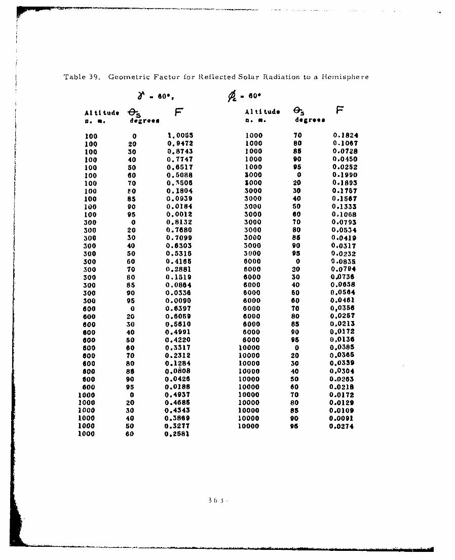
Table 39. Geometric Factor for Reflected Solar Radiation to a Hemisphere

- 60, - 600

Al ti tude F Al ti tud Fn. a. degrees no. . degrees

100 0 1.0055 1000 70 0.1824100 20 0.9472 1000 80 0.1067100 30 0.8743 1000 85 0.0728100 40 0.7747 1000 90 0.0450100 50 0.6517 1000 95 0.0252100 60 0.5088 3000 0 0.1990100 70 0.3505 3000 20 0.1893100 f:0 0.1804 3000 30 0.1757100 85 0.0939 3000 40 0.1567100 90 0.0184 3000 50 0.1333100 95 0.0012 3000 60 0.1068300 0 0.8132 3000 70 0.0793300 20 0.7680 3000 80 0.0534300 30 0.7099 3000 85 0.0419300 40 0.6303 3000 90 0.0317300 50 0.5315 3000 95 0.0232300 60 0.4165 6000 0 0.0835300 70 0.2881 8000 20 0.0794300 80 0.1519 8000 30 0.0736300 85 0.0864 6000 40 0.0858300 90 0.0336 6000 50 0.0564300 95 0.0090 6000 60 0.0461600 0 0.6397 6000 70 0,0356600 20 0.6059 6000 80 0.0257600 30 0.5610 6000 85 0.0213600 40 0.4991 6000 90 0.0172600 50 0.4220 6000 95 0.0136600 60 0.3317 10000 0 0.0385600 70 0.2312 10000 20 0.0365600 80 0.1284 10000 30 0.0339800 85 0.0808 10000 40 0.0304600 90 0.0426 10000 50 0.0263600 95 0.0188 10000 60 0.0218

1000 0 0.4937 10000 70 0.01721000 20 0.4685 10000 80 0.01291000 30 0.4343 10000 85 0.01091000 40 0.3869 10000 90 0.00911000 50 0.3277 10000 96 0.02741000 60 0,2581

3 6 3 -

Table 40. Geometric Factor for Reflected Solar Radiation to a Hemnisphere

Al ti tude F Altitude. Fa.s . degrees Ie s. degrees

100 0 1.0055 1000 70 0.1713100 20 0.9448 1000 80 0.0969100 30 0.8708 1000 85 0.0646100 40 0.7702 1000 90 0.0390100 50 0.6463 1000 95 0.0213100 60 0.5027 3000 0 0.1987100 70 0.3439 3000 20 0.1871100 80 0.1736 3000 30 0.1727100 85 0.0873 3000 40 0.1530100 90 0.0149 3000 50 0.1290100 95 0.0009 3000 60 0.1022300 0 0.8132 3000 70 0.0748300 20 0.7641 3000 80 0.0495300 30 0.7042 3000 85 0.0385300 40 0.6229 3000 90 0.0289300 50 0.5227 3000 95 0.0209300 60 0.4066 6000 0 0.0834300 70 0.2774 6000 20 0.0786300 80 0.1412 6000 30 0.0726300 85 0.0770 6000 40 0.0645300 90 0.0279 6000 60 0.0549300 95 0.0070 6000 60 0.0445600 0 0.6380 6000 70 0,0341600 20 0.6001 6000 80 0.0244600 30 0.5533 6000 85 0.0201600 40 0.489T 6000 90 0.0161800 50 0. 4113 6000 95 0.0127600 60 0.3201 10000 0 0.0384600 70 0. 2190 10000 20 0.0363600 80 0.1171 10000 30 0.0335600 85 0.0713 10000 40 0.0299600 90 0. 0361 10000 50 0.0257600 95 0.0154 10000 60 0.0212

1000 0 0. 4926 10000 70 0.01671000 20 0. 4635 10000 80 0.01241000 30 0.4274 10000 85 0.01051000 40 0. 3784 10000 90 0.00871000 50 0. 3179 10000 95 0.00911000 60 0. 2474

364-

Table 41, GeonietriC Factor for Reflected.- Solar Radiation to a H-emnisphere

Al tiitude 0F Al ti tde Fno so dg.. .m degrees 6a

100 0 1.0055 1000 70 0,1603100 20 0.9425 1000 to 0.0671

100 30 OjSS73 i000 so 0'.0644

100 40 0,7657 1000 go 0.0339100 s0 00409 1000 g5 0.0174

100 00 0.496? 3000 0 0.1984

100 70 0.3373 5000 90 0.1650

100 s0 0.1667 3000 30 0.1097

100 65 0.0806 3000 40 0#1401

100 g0 0. 0114 3000 50 0.1346100 95 0.000m 3000 00 0.0975

300 0 0.8133 3000 70 0.0703

300 20 0.7003 3000 so 0.0456

300 30 0.0985 3000 S6 0.0051

300 40 0.0615 3000 90 0.0360

300 so 0o8139 3000 g5 0,01,,

300 60 06.3966 6000 0 0.0833300 70 00 i..? 6000 20 0.0776300 s0 0.1306 0000 30 00.16

300 65 0.0076 0000 40 0.0831

300 90 0.0131 6000 50 0.0854

300 95 0. 0051 6000 60 0.0430

G00 0 0.1364 0000 70 0032O

o00 20 0.5943 0000 80 0.0431

"o00 30 0.6451 0000 as 0.0160

600 40 0.4801 6000 90 0.0151

-00 50 o.4007 0000 05 .o0011

600 00 003084 10000 0 0.0364

G00 70 0.3067 10000 20 0.0360

000 80 0.1057 10000 30 0.0331

o00 8a 0. 001O 100C 40 C.0394

000 90 0.0197 10000 s0 0.0235

600 95 0.0130 10000 00 0.0100

1000 0 0. 4916 10000 70 0.01,1

1000 g0 C.4534 10000 s0 0.0130

1000 30 0.4206 10000 a5 0.01011000 40 0.3701 10000 90 0.00381000 so 0. 301 10000 95 0.0061

1000 00 0.0 367

3 65

T able 42, C(eometric Factor for R.eflect ed Solar Radiation to a. Hemnispher'e

a 600 1500

Altit~ude At FAti tudeF

.n m. degrees n.o . degree@

100 0 1. 0055 1000 70 u.1522

100 20 0. 9407 1000 80 0.0799

100 30 0. 8647 1000 86 0.0504

100 40 O 7624 1000 90 0.0285

100 50 0. 6370 1000 96 0.0146

100 o0 0. 4922 3000 0 0.1982

100 70 0. 3325 3000 20 0.1834

100 80 0. 1617 3000 36 0.1675

100 85 0. 0759 5000 40 0.1465

100 90 0. 0089 3000 50 0.1214

100 95 0. 0003 3000 60 0,0941

300 0 0. 8132 3000 70 0.0069

300 20 0. 7573 3000 80 0,0427

300 30 0. 6'943 1000 85 G.0328

300 40 0. 8,101 3GO0 90 0,040

300 50 0 5075 3000 95 010170

300 60 0. 3894 80000 0 0.833

300 70 0.. 2589 6000 2U 0.0173

300 80 0. 1227 6000 30 0 .0707

300 85 0. 0608 ec00 40 0.0621

300 90 0. 0179 6000 50 0.062P

300 95 0. 0037 6000 60 0.0417

600 0 0. 6354 C0c0 70 0,0314

600 20 0. 5902 6000 80 0.0221

600 W0 0. 5402 6000 85 0.0180

600 40 0. 4738 8000 90 0.0143

OC 6 50 0. 3930 6000 9a 0.0112

630 50 0. 2999 10000 0 0.0584

600 70 0. 1978 10000 20 0,0358

600 80 0. 0974 10000 30 3.0328

"600 85 O. 054P 10000 40 0.0291

600 90 0. 0250 10000 30 0.0248

600 95 0. 0095 10000 00 0.0202

1000 0 0. 4908 10000 70 0.0137

1000 20 0. 4548 10000 80 0.0116

1000 3;) 0. 4157 10000 85 o. 3097

1000 40 0. 3640 13000 90 0.0080

1000 5u 0. 3012 10000 96 0.0665

1000 60 O 7288

Table 43. Geometric Factor foi- Reflected Solar Radiation to a Hemisphere

*60180

Altitude F Al titude o: Fn.o . degrees n. m. degrees

100 0 1. 0055 1000 70 0.1492

100 20 0. 9401 1000 80 0.0773100 30 0.8838 1000 85 0.0482100 40 0. 7612 I000 90 0.0269100 s0 0.6356 1000 95 0.0136100 60 0. 4906 3000 0 0.1982100 70 O. 3307 3000 20 0.1829100 80 0. 1599 3000 30 0.1667100 85 0. 0742 3000 40 0.1455100 90 0. 0079 3000 50 0.1203100 95 o. 0003 3000 60 0.0929500 0 0. 8132 3000 70 0.0657300 20 0. 7563 3000 80 0.0417300 30 0. 6928 3000 85 0.0317300 40 0. 6082 3000 90 0.0232300 50 0, 5051 3000 95 0.0164300 60 0. 3867 6000 0 0.0833300 70 0.2560 6000 20 0.0771300 80 0.1199 6000 30 0.0704300 85 0.0581 6000 40 0.0618300 90 0.0164 5000 60 0.0518300 95 0.0032 6000 60 0.0413600 0 0.6352 6000 70 0,0310600 20 0.5888 6000 80 0.0217600 30 0.5383 6000 85 0.0177600 40 0. 4714 6000 90 0.0140800 60 0.3902 6000 95 0.0109800 60 0.2969 10000 0 0.0384

o00 70 0. 1946 10000 20 0.0357600 80 0 0. 0944 10000 30 0.0327600 85 0.0523 10000 40 0.0289600 90 0.0233 10000 50 0.0246900 95 0.0086 10000 60 0.0201

1000 0 0. 4907 10000 70 0.015,1000 20 0.4536 10000 80 0.01151000 30 0. 4140 10000 85 0.00961000 40 0. 3618 10000 90 0.00791000 50 0. 2986 10000 95 0.00641000 60 Oo 2260

- 367-

Table 44. Geometric Factor for Reflected Solar Radiation to a. Hemisphere

go 09 9" -0"

Altitude -9ý F Alt.i tude F0.1 . degrees a. so degrees

100 0 ýL. 7672 1000 70 0.1471100 20 0C7265 1000 80 0.0917100 n0 0.6725 1000 85 0.0853100 40 0.5981 1000 go 0.0422100 50 0.5055 1000 95 0.0246100 60 C.3976 3000 0 0.1304100 70 0.2776 3000 20 0,1328100 80 0.14PS2 3000 30 0.1249100 SG 0.0819 -009 40 0.1132

100 90 0.0201 3000 60 0.0082100 96 0.0016 3000 60 0.0806300 0 0.6026 3000 70 0.0617

300 20 P.575Z 3000 80 0,0429300 30 0.5351 3000 85 0.0343300 40 0. 4786 3000 90 0.0264300 50 0.4076 3000 95 0.0197

300 60 0.3242 6000 0 0.0563300 70 0.2303 6900 20 0.0547

300 P0 0.1293 6000 30 0.0514300 85 0.0793 6000 40 0.0465300 90 0.0348 6000 60 0.0405300 96 0.0101 00G0 60 0.0337600 0 0.4851 8000 70 0002656OC 20 0. 4414 8000 80 0.0195600 30 0. 4178 6000 83 0.0103660 40 0.3756 6000 90 0.0133S00 50 0.3220 6060 95 0.0106600 60 0. 2584 10000 0 0.0258000 70 0.1867 10000 20 0.0249600 80 0.1112 1U000 30 0.0234500 85 0.0741 10000 40 0.0212800 90 0.0418 10000 50 0.0188

600 95 0.0196 10000 60 0.01551000 0 0.3519 10000 70 0.01241000 20 0. 3404 10000 80 0.00941000 30 0.3189 10000 85 0.00801000 40 0,278 1o000 90 Cooo61000 GO 0. 2476 10000 95 0.0055W1OOo 680 0 2002

-368,

!-•&

Table 45. Geometric Factor for Reflected Solar Radiation to a Hemisphere

- 90"A 30"

Al tirtude F Altitude.* MO degree° U.* . degree.

100 0 0.7672 1000 70 T 1437

100 20 o.7257 1000 so 0.0886

100 30 0.6714 1000 85 0.0628

100 40 0.5967 1000 90 0.0403

100 s0 0.5039 1000 9g 0.0234

100 60 0.3957 3000 0 0.1363

100 70 0.2755 3000 20 0.1322

100 80 0.1461 3000 30 0.1240

100 85 0.0799 3000 40 0.1120

100 90 0.0191 3000 50 0.0968

100 95 0.0014 3000 60 0.0792

300 0 0.6026 3000 70 0.0602

300 20 0.5741 3000 80 0.0417

300 30 0.5333 3000 85 0.0332

300 40 0.4163 3000 90 0.0256

300 so 0.4049 3000 95 0.0189

300 60 0.3211 6000 0 0.0563

300 70 0.2270 6000 20 0.0545

300 80 0.1260 6000 30 0.0510

300 85 0.0T64 6000 40 0.0461

300 90 0.0330 6000 50 0.0400

300 95 0.0095 8000 60 0.0332

600 0 0.4644 6000 70 0,0260

600 20 0.4453 0000 80 0.0191

600 s0 0.4153 6000 85 0.0159

600 40 0.3726 6000 90 0.0130

800 s0 0.3186 8000 95 0.0103

600 60 0.2547 10000 0 0.0258

000 70 0.1829 10000 20 0.0248

600 80 0.1075 10000 30 0.0232

600 85 0.0712 10000 40 0.0210

600 90 0.0398 10000 50 0.0183

800 95 0.0185 10000 60 0.0153

1000 0 0.3514 10000 70 0.0123

1000 20 0.3397 10000 80 0.0093

1000 30 0.3107 10000 85 0.0079

1000 40 0.2851 10000 90 0.0066

1000 s0 0.2448 10000 95 0.0054

1000 80 011969

- 3 69 -

Table 46. Geometric Factor for Reflected Solar Radiation to a Hemisphere

g 0,e. 600

Al tittude F Altitude G Fa. *. degree no. i. degrees

:100 0 0.7672 1000 70 0.1343

100 20 0.7237 1000 80 0 0803

100 30 0,6685 1000 85 0.0558

100 40 0.5929 1000 90 0.0352

100 50 ,1.4993 1000 95 0.0201

100 60 0.3906 3000 0 0.1360

100 70 0.2700 3000 20 0.1303

100 80 0.1403 3000 30 0.1214

100 85 0.0744 3000 40 0.1088

100 90 0.0161 3000 50 0.0931

100 95 0. 0012 o000 60 0.0752

300 0 0.6026 3000 70 0.0064300 20 0.5708 3000 80 0.0384300 30 0.5285 3000 85 0.0303300 40 0. 4701 3000 g0 0.0232

300 50 0.3975 3000 95 0.0170

300 60 0.3127 6000 0 0.0562

300 70 0.2179 6000 20 0.0538

300 80 0.1170 6000 30 0.C501

300 85 0.0684 6000 40 0.0450

300 90 0.0281 6000 50 0.0387

300 95 0.0079 6000 80 0.0318

600 0 0.4628 8000 70 0,0247

600 20 0.4403 6000 80 0.0180

600 30 0.4086 6000 85 0.0149

000 40 0).3646 6000 90 0.0121600 50 ;.3095 6000 95 0.0096

600 60 0. 2448 10000 0 0.0258

600 70 0.1725 10000 20 0.0246

600 80 0.0980 10000 30 0.0229

800 85 0.0631 10000 40 o.0206

600 90 0.0343 10000 50 0.0179

600 95 0.0156 10000 60 o.0149

1000 0 0. 3504 A0000 70 0.0118

1000 20 0. 3343 10000 80 0.0089

1000 30 0. 3109 10000 85 0.0075

1000 40 0. 2779 10000 90 0.0083

1000 50 0. 2366 10000 95 0.0051

1000 80 0,, 1878

1 7

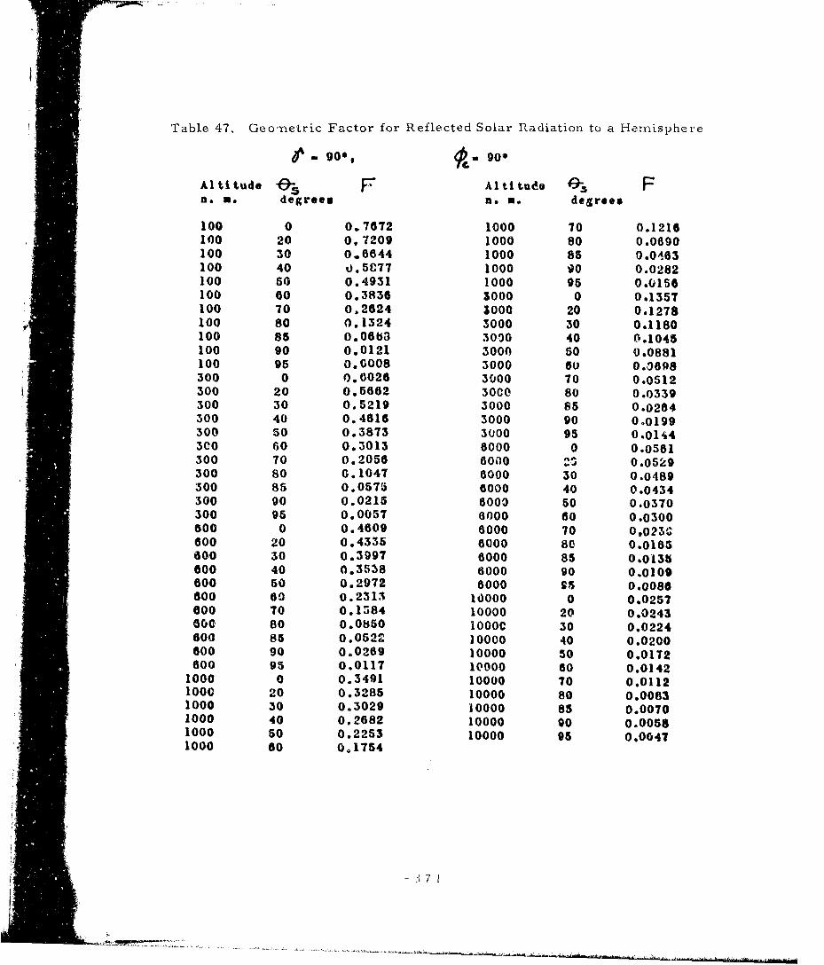
Table 47. Geometric Factor for Reflected Solar Radiation to a Hemisphere

&0- go*, (; 900

Altitude F Al titu.e 4 Fn. a. degrees n. m. degrees

100 0 0.7672 1000 70 0.1216100 20 0.7209 1000 80 0.0690100 30 0.6844 1000 85 0.0483100 40 0.5C77 1000 g0 0.0282100 50 0.4931 1000 95 0.0156100 00 0.3836 3000 0 0.1357100 70 0.2624 3000 20 0.1278100 80 0.1324 3000 30 0.1180100 85 0.0663 3010 40 0.1045100 90 0.0121 3000 50 0.0881100 95 0.0008 3000 60 0.0698300 0 0.0026 3000 70 0.0512300 20 0.5662 3000 80 0.0339300 30 0.5219 3000 85 0.0204300 40 0.4616 3000 90 0.0199300 50 0.3873 3000 95 0.0144300 60 0.3013 6000 0 0.0561300 70 0.2056 6000 0.0529300 80 G.1047 6000 30 0.0489300 85 0.0575 6000 40 0.0434300 90 0.0215 6000 50 0.0370300 95 0.0057 6000 60 0.0300600 0 0.4609 8000 70 0,023C600 20 0.4335 6000 80 0.0165600 30 0.3997 6000 85 0.0135600 40 0.3538 6000 90 0.0109600 50 0.2972 6000 ps 0.0088600 60 0.2313 10000 0 0.0257600 70 0.1584 10000 20 0.02438oo 80 0.0850 1000C 30 0.0224600 85 0.0522 10000 40 0.0200600 90 0.0269 10000 50 0.0172600 95 0.0117 10000 60 0.0142

1000 0 0.3491 10000 70 0.01121000 20 0.3285 10000 80 0.00831000 30 0,3029 10000 85 0.00701000 40 0.2682 10000 90 0,00581000 50 0.2253 10000 95 0.00471000 60 0.1754

S7 I

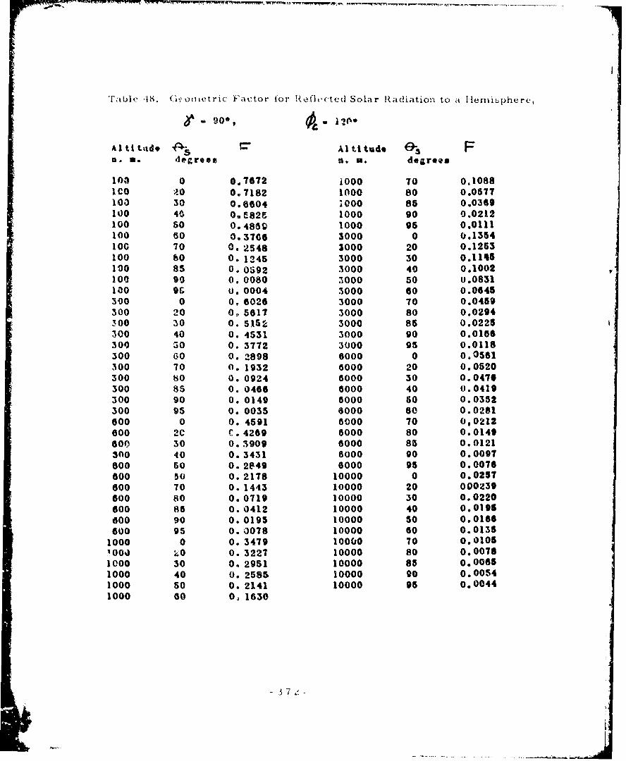
"Table .18. (1vo uetric Factor for Reflected Solar Radiation to a I-Ierniiphere,

S- 00g, &- 12%0

AIti td. Al titude 01S Fn. a. degrees :.n . degrees

100 0 0.7672 i000 70 0.10881c0 0 0.7182 1000 80 0.0577100 30 0.6604 "OO0 85 0.0369100 4 . 0,,825 1000 90 0.0212100 s0 0.486g 1000 95 0.0111100 10 0.3706 3000 0 0.1354lOG 70 0. 2548 3000 20 0.1253100 80 0. 1245 3000 30 0.1145100 85 O- 0592 3000 40 0.1002100 90 0. 0080 3000 50 o.0831100 9& U. 0004 3000 60 0.0645300 0 0, 6026 3000 70 0.0459300 20 0, 5617 3000 80 0.0294300 30 0. 5152 3000 85 0.0225300 40 0. 4531 3000 90 0.0166300 50 0. 3772 3000 95 0.0118300 60 0. 2898 6000 0 0.0561300 70 0. 1932 6000 20 0.0520300 80 0. 0924 8000 30 0.0416300 85 0. 0460 6000 40 0.0419300 90 0. 0149 6000 50 0.0352300 95 0. 0035 6000 60 0.0281600 0 0. 4591 6000 70 0,0212600 2C C. 4269 6000 80 0.0149600 30 0. 3909 6000 85 0.0121300 40 0. 3431 6000 90 0.009?600 60 0. 2849 6000 95 0.0076600 50 0. 2178 10000 0 0.0257600 70 0. 1443 10000 20 000239600 80 0. 0719 10000 30 0.0220600 85 0. 0412 10000 40 0.0195600 90 0. 0195 10000 SO 0.0166600 95 0. 0078 10000 60 0.0135

1000 0 0. 3479 10000 70 0.0105'000 k0 0. 3227 10000 80 0.00781000 30 0. 2951 10000 85 0.00651000 40 0. 2585 10000 90 0.00541000 50 0. 2141 10000 95 0.00441000 60 0 1630

-3 7Z-

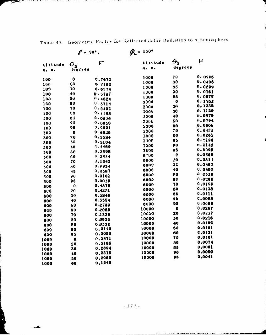
Table 49. Geometric F tfor R.efl.cted Jolar R-adilitio: to a HemnisPlhere

( g. 9oo, 150"

Al ti tude I&I 1t~.%tuds 05 Fn. M. degrees o.m. degrees

100 0 0.7672 1000 70 0.0945

GO 20 0.7182 1000 8s 0.0495

101 30 0.-574 1000 80 0.0296

100 40 .G78 1000 90 0.0181

100 5 0.4824 1000 96 O.1O0t

IGO 60 0.3714 3000 0 0.1352

100 70 0.2492 1000 20 0.1239

100 0 0. -i88 3000 30 0.1120

100 83 6.05.1 3000 40 (1.0970

100 90 0.00r0 30(0 50 0o0794

100 95 9.0001 300O 00 0.0800

300 0 0.-026 3000 70 0.0421

300 i0 0.5584 3000 80 0.0261

300 30 0.5104 3000 85 0.P196

300 40 1)4469 3000 PO U.0142

300 50 0.3698 3000 95 0.0099

300 60 0 20i4 6100 0 0.0560

300 70 d.1842 6000 20 0.0514

300 80 0,0834 6000 3c 0.0461

300 85 0.0387 6000 40 0.0401

300 90 0.0101 6000 c0 0.0339

300 95 0.0019 6000 60 0.0688

600 0 0.4579 6000 70 0,010

600 20 0.4221 0000 80 0.0138

600 30 0.3846 6000 85 0.0111

600 40 0.3354 6000 90 0.0088

600 60 0.2760 6000 95 0.0068

600 80 0.2080 10000 0 0.0257

600 70 0.1339 0MOO 20 0.023?

600 80 0.0623 10000 30 0.0216

600 85 0.0332 10000 40 0.0190

600 90 0.0140 10000 50 0.0161

600 95 0.0050 10000 60 0.0131

1000 0 0.3471 10000 70 0.0101

1000 20 0.3185 10000 80 0.0074

1000 30 0.2894 10000 65 0.0061

1000 40 0.2515 10000 90 0.0050

1000 50 0.2060 10000 95 0.0041

1000 60 o,1640

- 7 37 -

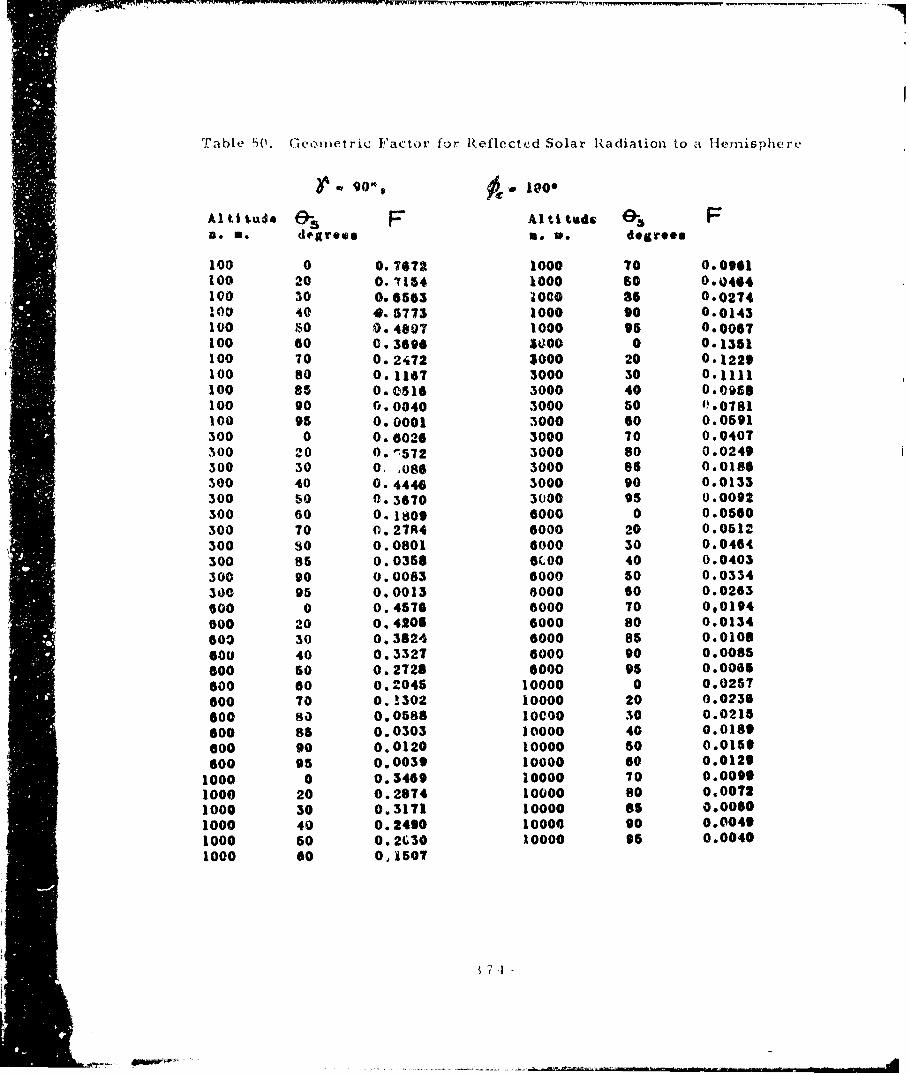
Table 50. GicoIetric Factor fur Reflected Solar Radiation to a Hemisphere

A1lti tude - F Al tttuds 0.3 Fn. m. dearee# s.o . degrees

100 0 0.7672 1000 T0 0.0901100 20 0.(154 1000 60 0.0464100 30 0.0503 1000 85 0.0274100 40 4. 5773 1000 90 0.0143100 so 0.4807 1000 95 0.0067100 60 0.3690 Z000 0 0.1351100 TO 0.2472 3000 20 0.1220100 8o 0.1107 3000 30 0.1111100 as 0.0516 3000 40 0.0958100 0o 0.0040 3000 s0 0.0781

oo 95 0. o0001 3000 60 0.0591300 0 0.6026 3000 70 0.0407300 20 0.-572 3000 80 0.0249300 30 0. ,080 3000 85 0.0186300 40 0.4446 3000 90 0.0133300 50 0.3670 3000 95 0.0092300 60 0.1809 6000 0 0.0500300 70 0.27R4 6000 20 0.0512300 so 0.0801 6000 30 0.0464300 85 0.03568 6L00 40 0.0403300 90 0.0083 6000 50 0.0334300 95 0.0013 8000 60 0.0263S00 0 0.4576 6000 70 0,0194S00 20 0.4.206 6000 80 0.0134600 30 0.3824 6000 85 0.0108000 40 0.332? 6000 90 0.0085600 60 0.2728 6000 95 0.0085600 60 0.2045 10000 0 0.0257600 70 0.3302 10000 20 0.0236600 80 0.0588 1Ooo0 30 0.0215600 85 0.0303 10000 40 0.0189

600 90 0.0120 10000 50 0.0159600 95 o.0039 10000 60 0.0129

1000 0 0.3469 10000 70 0.00901000 20 0.2874 10000 80 0.00721000 30 0.3171 10000 aS 00060

1000 40 0.2490 10000 90 0.00491000 50 0.2(30 10000 95 0.00401000 s0 0,1507

MI| II

qI.B

-i - • . t- -~

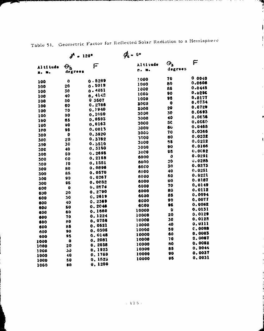
Table 51. Geometric Factor for Reflected Solar Radiation to a Hemisplkerc

. 120" A 0*

Al ti ttde F? Al ti ide Fso so degrees re a* degrooz

100 0 0.5289 '000 70 0 0940

100 20 0.5019 1000 80 0°0608

100 30 0.4851 1000 a6 0.0445

100 40 0).4142 1000 90 0.0296

100 60 0 3507 1000 95 0.017?

100 60 0.2766 lo0o 0 0.0734

100 70 0.)940 3000 20 0.0729

100 s0 0.1050 3000 30 0.0693

100 85 0.0593 3000 40 0.0036

100 90 0.0163 3000 SC 0.086•

100 95 0.0013 3000 6S 0.0468

300 0 0.3920 3000 70 0.0366

300 20 0.3762 U000 80 0.0232

390 30 0.5510 3000 85 0.0212

300 40 0.3150 3000 90 0.0166

300 50 0.2695 3000 95 0.0062

300 Go 0.2158 6000 0 0.0291

300 10 0.1551 6000 20 0.0288

300 80 0.0896 6000 30 0.0273

300 85 0.0570 6000 40 0.0251

300 90 0.0267 6000 s0 0.0221

300 95 0. 0032 6000 60 0.0187

600 0 U. 2874 6000 70 0,0149

G00 20 0.2790 6000 80 0.0112

600 30 0.2619 6000 85 0.0094

600 40 0.2369 6000 90 0.0077

600 60 0.2040 6000 95 0.0062

600 60 o. 1660 10000 0 0.0131

600 70 0.1224 10000 20 0.0129

600 0 0.0756 10000 30 0.0122

600 85 0. 0521 10000 40 0.0111

o00 90 o. 0306 10000 50 C.0098

G00 95 0.0148 10000 60 0.0083

1000 0 o. 2081 10000 70 0.0061

1000 20 0. 2038 10000 80 0.0052

1009 30 0. 1923 10000 86 0.0044

1000 40 0. 1760 10000 90 0.0037

1000 50 0. 1523 10000 95 0.0031

1000 60 0, 1250

3 7 j

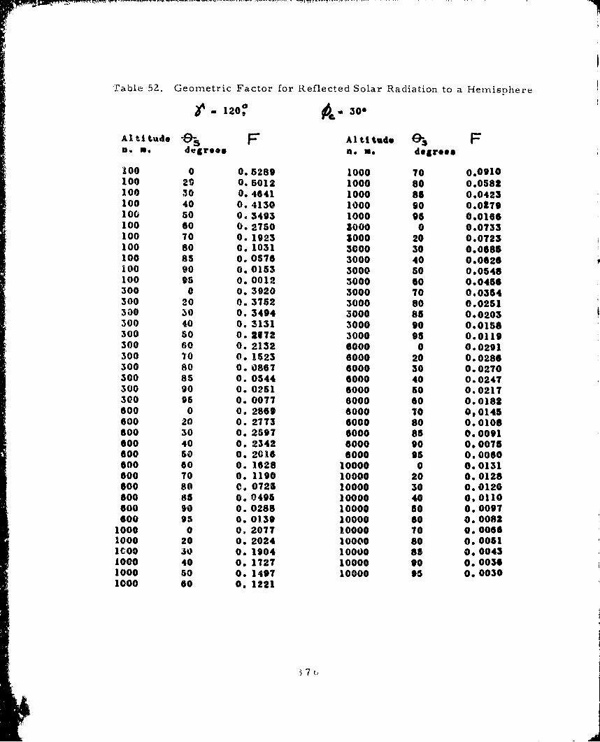
Table 52. Geometric Factor for Reflected Solar Radiation to a Hemisphere

1 120' o 30

Altirtde F" Altitud, a3 Fn. a. degrtes n. no degrees

100 0 0.5289 1000 70 0.0910100 20 0.5012 1000 80 0.0582100 30 0. 4641 1000 85 0.0423100 40 0. 4130 1000 90 0.027910 50 s0.3493 1000 95 0.0166100 60 0.2750 3000 0 0.0733100 70 0. 1923 3000 20 0.0723100 80 0. 1031 3000 30 0.0685100 85 0. 0576 3000 40 0.0626100 90 0.0153 3000 50 0.0548100 95 0. 0012 3000 60 0.0456300 0 0, 3920 3000 70 0.0354300 20 0. 3752 3000 80 0.0251300 s0 0. 3494 3000 85 0.0203300 40 0. 3131 3000 90 0.0158300 50 0. 2172 3000 95 0.0119300 60 0. 2132 6000 0 0.0291300 70 0. 1523 6000 20 0.0286300 80 0. 0867 6000 30 0.0270300 85 0. 0544 6000 40 0.0247300 90 0. 0251 6000 50 0.0217300 96 0. 0077 6000 60 0.0182600 0 0. 2869 6000 70 0,0145600 20 0. 2773 6000 80 0.0108600 30 0. 2697 6000 85 0.0091600 40 0. 2342 6000 90 0.0075600 50 0. 2016 6000 95 0.0060600 60 0. 1628 10000 0 0.0131600 70 0. 1190 10000 20 0.0128600 80 C, 0725 10000 30 0.0120600 85 0.0495 10000 40 0,0110000 90 0.0288 10000 50 0.0097600 95 0.0139 10000 60 0.0082

1000 0 0. 2077 10000 70 0. 00661000 20 0. 2024 10000 80 0. 005110oo 30 0. 1904 10000 85 0. 00431000 40 0. 1727 10000 90 0. 00361000 50 0. 1497 10000 95 0. 00301000 60 0. 1221

:'- 37u

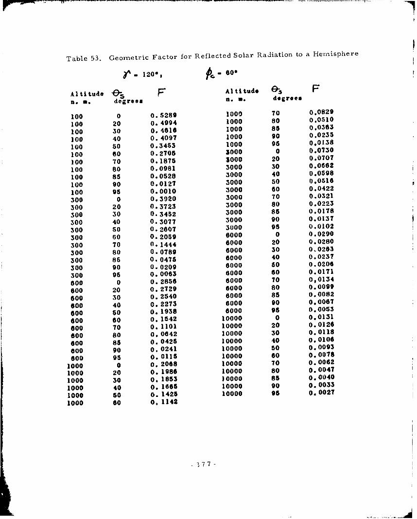
Table 53. Geometric Factor for Reflected Solar Radiation to a Hemisphere

Al ti tude F Al tud . Fn. m. degrees n. s. degrees

100 0 0.5289 1000 70 0.0829

100 20 0. 4994 1000 80 0.0510

100 30 0.4616 1000 85 0.0363

100 40 0. 4097 1000 90 0.0235

100 50 0.3453 1000 95 0.0138

100 60 0.2705 3000 0 0.0730

100 70 0.1875 3000 20 0.0707

100 80 0.0981 3000 30 0.0862

100 85 0.0528 3000 40 0.0598

100 90 0.0127 3000 50 0.0516

100 95 0.0010 3000 60 0.0422

300 0 0.3920 3000 70 0.0321

300 20 0.3723 3000 80 0.0223

300 30 0.3452 3000 85 0.0178

300 40 0.3077 3000 90 0.0137

300 50 0.2607 3000 95 0.0102

300 60 0.2059 6000 0 0.0290

300 70 0.1444 6000 20 0.0280

300 80 0.0789 6000 30 0,0263

300 85 0.0475 6000 40 0.0237

300 90 0.0209 6000 60 0.0206

300 95 0. 0063 6000 60 0.0171

600 0 0. 2856 6000 70 0,0134

600 20 0. 2729 6000 80 0.0099

600 30 0. 2540 6000 85 0.0082

600 40 0. 2273 6000 90 0.0067

600 50 0. 1938 6000 95 0.0053

600 60 0. 1542 10000 0 0.0131

G00 70 0. 1101 10000 20 0.0126

600 80 0. 0642 10000 30 0.0118

600 85 0. 0425 10000 40 0.0106

600 90 0. 0241 10000 50 0.0093

600 95 o.0115 10000 60 0.0078

1000 0 0. 2068 10000 70 0.0062

1000 20 0. 1986 10000 80 0.0047

1000 30 0. 1853 30000 85 0.0040

1000 40 0. 1665 10000 90 0.0033

1000 50 0. 1425 10000 95 0.0027

1000 60 0. 1142

), •7 7-

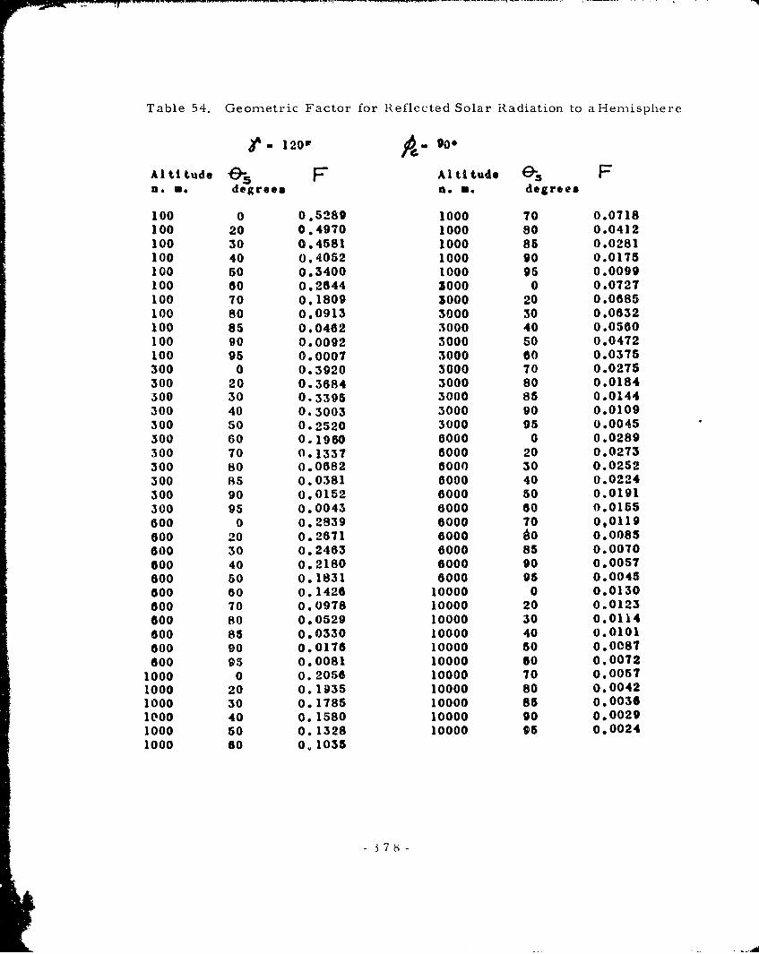
Table 54. Geometric Factor for Reflected Solar Radiation to a Hemisphere

d-12 0P A 9000*Al ti t.ude 5 F Al titude ( Fn.o . degrees n. m. degrees

100 0 0.5289 1000 70 0.0718100 20 0.4970 1000 80 0.0412100 30 0.4581 1000 85 0.0281100 40 0.4052 1000 90 0.0175100 50 0.3400 1000 95 0.0099100 60 0.2644 3000 0 0.0727100 70 0.1809 3000 20 0.0685100 80 0.0913 3000 30 0.0632100 85 0.0462 3000 40 0.0560100 90 0.0092 3000 50 0.0472100 95 0.0007 3000 60 0.0375300 0 0.3920 3000 70 0.0275300 20 0.3684 3000 80 0.0184300 30 0.3395 3000 85 0.0144300 40 0.3003 3000 90 0.0109300 50 0.2520 3000 95 0.0045300 60 0.1960 6000 0 0.0289300 70 0.1337 6000 20 0.0273300 80 0.0682 6000 30 0.0252300 85 0.0381 6000 40 0.0224300 90 0.0152 6000 50 0.0191300 95 0.0043 6000 60 0.0155600 0 0.2839 6000 70 0,0119600 20 0.2671 6000 g0 0.0085600 30 0.2463 6000 85 0.0070600 40 0.2180 6000 90 0.0057

800 50 0.1831 6000 95 0.0045600 60 0.1426 10000 0 0.0130600 70 0.0978 10000 20 0.0123800 80 0.0529 10000 30 0.0114600 85 0.0330 10000 40 0.0101600 90 0.0176 10000 50 0.0087600 95 0.0081 10000 60 0.0072

1000 0 0.2056 10000 70 0.00571000 20 0.1935 10000 80 0.00421000 30 0.1785 10000 85 0.00361000 40 0.1580 10000 90 0.00291000 50 0.1328 10000 95 0.00241000 60 0.1035

- 37 -

Table 55. Geometric Factor for Reflected Solar Radiation to a '.-Ienisphere

0. 120*, 9- 1200

Altitude F Altitude o Fn. m. degrees I.e . degrees

100 0 0.5289 1000 70 0.0608100 20 0.4946 1000 80 0.0314100 30 0.4544 1000 85 0.0108100 40 0.4007 1000 90 0.0114100 50 0.3346 1000 95 0.0060100 60 0.2684 3000 0 0.0725100 70 0.1703 3000 20 0.0664100 80 0.0845 3000 30 0.0602100 85 0.0398 3000 40 0.0523100 90 0.0057 MOO so 0.0429100 95 0°0004 3000 60 0.0328300 0 0.3920 3000 70 0.023C300 20 0.3645 L000 80 0.0145300 30 0,O!3f 3000 85 0.0U10300 40 0.2029 3000 90 0.0080300 so 0.2432 .OCO 95 0.0057300 60 0.1861 6000 0 0.0288300 70 0.1230 6000 20 0.0265300 80 U.0578 60J0 30 0.0241300 85 0.0287 6000 40 0.0210300 90 0.0095 6096 50 0.0175300 95 0.0024 6000 60 0.0139600 0 0.2823 6000 70 0,0103600 20 0.2513 6000 80 0.0072600 30 0.238T 0000 85 0. 0058600 40 0.2088 6a)00 90 0.0046600 50 0.1725 6000 95 0.0036600 60 0.1309 10000 0 0.0130600 70 0.0856 10000 20 0.0120600 80 0.0416 10000 30 0.0110600 85 0.0235 10000 40 0.0096600 90 0.0112 10000 50 0.0082600 95 0.0047 10000 00 0.0066

1000 0 0.2046 10000 70 0.00511000 20 0.1885 10000 80 0.00371000 30 0.1717 10000 5 0, 00311000 40 0.1497 10000 90 0.00201000 50 0.1231 10000 9 0.00211000 60 0 0927

1 7 9

Table 56. Geometric Factor for' Reflected Solar Radiation to a Hemisphere

1200, 04- 101

Al ti tud* Altitude e-3 FU. so 4agreis Do Xk. degre*&

100 0 o.5280 1000 TO 0,652T100 20 0.4929 1000 80 0.0243100 30 G.4520 1000 8 0.0139100 40 o.3974 1000 90 0.0070100 do 0.3397 1000 95 0.0032100 60 0.2639 S000 0 0.0723100 70 0.1695 3000 20 0.0048100 80 0.0794 3000 30 0.0581100 8a 0.0348 3000 40 0,0496100 90 0.00fl 3000 s0 0.0397100 95 0.0001 3000 00 0.0294300 0 0.3920 3000 70 0.0191300 20 0.3618 3000 80 0.0116300 30 0.3296 3000 85 0.0085300 40 0.2875 3000 90 0.0060300 50 0.2388 3000 95 0.0041300 00 0.1188 0000 0 0.0288300 70 0.1152 6000 20 0.0258300 80 0.0498 0000 30 0.0233300 85 0.0218 8000 40 0.0200300 90 0.0053 8000 50 0.0184300 96 0.0010 6000 60 0.0127800 0 0.2813 0000 70 0,0092600 20 0.2572 6000 80 0.0062000 s0 0.2332 6000 85 0.0049600 40 0.2020 6000 90 0.0338600 50 0.1648 6000 95 0.0029600 80 0.1224 10000 0 0.0130600 70 0.0788 10000 20 0.011S600 80 Q.0333 10000 30 0.0107600 85 0.0166 10000 40 0.0093800 90 0.0065 10000 50 0.0078600 95 0.0022 10000 60 0.0062

1000 0 0.2039 10000 70 0.004?1000 20 0.1849 10000 so 0.00341000 30 0.1668 10000 as 0.00281000 40 0.1436 10000 90 0.00231000 50 0.1160 10000 0S 0.00181000 s0 0.084V

38G-

.1

Table 57. Geometric Factor for Reflected Solar Radiation to a Hemisphere

S- 120o0 ,. 1800

Altitude e F Altitd. Fs. s. dogrooe s.o . degrees

100 0 0.5289 1000 70 00497

100 20 0.4922 1000 8o 0.0216

lOO 30 0.4511 1000 8a 0.0117

100 40 0.3962 1000 g0 0.0054

100 50 0.3292 1000 95 0.0022

100 60 0.2523 3000 0 0.0723

100 70 0,1677 3000 20 0.0643

100 80 0.0776 3000 30 0.0573

100 85 0.0330 3000 40 0,0485

100 90 0,0022 3000 50 0,086

100 0g 0.0000 3000 60 0.0282

300 0 0.3920 3000 70 0.0185

300 20 0.3605 3000 80 0.0106

306 3C 0.3280 3000 8a 0.0076

300 40 0.285f' 3000 90 0,0052

300 50 0.2344 3000 98 0.003M

300 60 0.1161 6000 0 0.0288

300 70 0.1123 6000 20 0.0257

300 80 0.0469 6000 30 0.0230

300 85 0.0192 6000 40 0-0197

300 90 0.0037 6000 s0 0.0160

300 95 0.0005 6000 60 0-0123

600 0 0.2811 6000 70 090088

600 20 0.2558 6000 80 0-0058

600 30 092313 6000 85 0-0046

600 40 0.1907 6000 90 0.0036

600 s0 0.1620 6000 95 0-0027

600 60 0.1194 10000 0 04130

G00 70 0.0734 10000 20 0.0117

600 80 0*0302 10000 30 0.0106

600 85 0.0141 10000 40 000092

600 90 0.0048 10000 50 0.0076

6oo 95 0.0013 10000 60 0.0060

1000 0 0.2037 10000 70 0,0046

1000 20 0.1837 10000 so 0.0032

1000 30 0.1650 10000 Sf 0.0021

1000 40 0.1414 10000 (10 0.0022

1000 50 0.1135 10000 06 0.0017

1000 60 0*0821

-381-

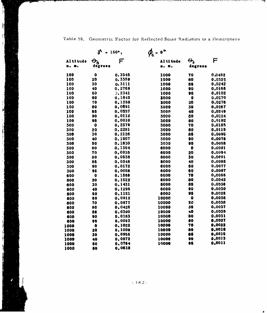
Table 58. Geometric Factor for Reflected Solar Radiationi to a. HerriisDhere

Altitude 8r F Altitude I Fas as degrees so no degrees

100 0 0.3545 1000 70 0.0482100 20 o.3359 1000 80 0*0322100 30 0,3111 1000 85 0,0242100 40 0.2768 1000 90 0.0186100 50 ),2341 1000 95 0o0102100 60 0.1842 3000 0 0.0270100 70 0,1288 3000 20 040276100 so 0.0691 3000 30 0.0267100 85 0.0337 3001M 40 0,0249100 00 0o0I12 3000 50 0.0224100 95 0.0010 3000 60 0.0192300 0 0.2379 3000 70 0,0155300 20 0.2281 3000 80 0.0115300 30 0. 2120 3000 85 0.0095300 40 0. 1907 3000 90 0.,0076300 50 0.1630 3000 95 0.0058300 60 0. 1304 6000 0 0.0091300 70 0.0935 6000 20 0100)94300 80 000538 6000 30 0.0091300 85 0.0348 6000 40 0.0085300 90 0.0172 6000 so 0.0077300 95 0.0056 6000 60 0.0067600 0 0. 1566 0000 T0 0,0055600 20 0.1522 6000 s0 0.0042600 30 0. 1431 6000 85 0.0036600 40 0: 1295 6000 90 0.0030600 s0 0.1121 6000 95 0o0025600 60 0.0912 10000 0 0.0o38

600 70 0.0677 10000 to 0.0038600 80 0.0425 10000 s0 0,0037

6o00 8 0.0300 10000 40 0,0035

600 90 0.0183 10000 s0 0.0031

600 95 0.0093 10000 60 0.0027

1000 0 O. O022 10000 70 0.00221000 20 0.1001 10000 o0 000011000 30 0.0955 10000 85 0.00151000 40 0.0872 10000 90 .OO31000 50 0.0764 10000 98 0.0011

1000 g0 0.0631

-18 2

Table 59. Geometric Factor for Reflected Solar Radiation to a Hemisphere

SICOf, 300

AltUtude F Altitude FOI. a, degrees I.s . degrees

100 0 *.3545 1000 70 0.0465

100 LO 0.3355 1000 80 0.03'6100 30 0.3105 1000 85 0.0229100 40 0,2761 1000 g0 0.0157100 50 0.2332 1000 95 0.0096100 60 0.1833 5000 0 0.0270100 70 0.1278 5000 20 0.0273100 80 0.0680 3000 30 0.0262100 85 0.0377 3000 40 0,0243100 90 0.0107 3000 50 0.0217100 95 0.0009 3000 60 0.0185300 0 0.2379 3000 70 0.0148300 20 0.2274 3000 80 0.0109300 30 0.2117 3000 8a 0.0090300 40 0.1896 3000 90 0,0071300 50 0.1617 3000 95 0.0055300 60 0.1288 6000 0 0.0091300 70 0.0918 6000 20 0.0092300 80 0.0522 6000 30 0.0089300 85 0.0333 6000 40 0.0083300 90 0.0163 6000 50 0.0075300 95 0.0053 6000 60 0.0064600 0 0.1562 6000 70 0,0053600 20 0.1512 6000 80 0.0040600 30 0.1418 6000 85 0.0034600 40 0.1280 6000 90 0.0029600 s0 0.1104 6000 95 0-0023600 @0 0.0893 10000 0 0.0038o00 70 0.0657 10000 20 0.0038o00 80 0.0407 10000 30 0.0036

600 85 0.0285 10000 40 0@0034600 90 0.0173 10000 50 0 0030600 95 0.086 10000 60 0.0026

1000 0 01019 10000 70 0.00221000 20 0.0999 10000 80 0100171000 30 0.0943 10000 85 0.00151000 40 0.0859 10000 90 0,00121000 50 0.0748 10000 96 0A0101000 60 0.0615

-383 -

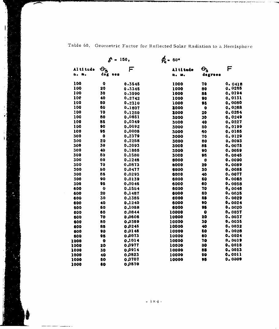
Table 60. Geometric Factor for Reflected Solar Radiation to a Hemisphere

- 150, 04- 600

Alti tude F Altitude 9 Fa* m. dog soe I. w. degroes

100 0 0.3545 1000 70 O 0418100 20 0.3345 1000 80 0,0285100 30 0.3090 1000 85 0,0194100 40 0.2742 1000 90 0.0131100 50 0.2310 1000 95 0.0080100 60 0.1807 3000 0 0.0268100 70 0.1250 3000 20 0.0264100 80 0.0651 3000 30 0.0249100 85 0.0349 3000 40 0.0227100 90 0.0092 3000 50 0.0199100 95 0.0008 3000 80 0.0165300 0 0.2379 3000 70 0.0129300 20 0.2258 3000 80 0.0093300 30 0.2093 3000 85 0.0075300 40 0.1865 3000 90 0.0059300 50 0.1580 3000 95 0.0045300 60 0.1246 6000 0 0.0090300 70 0.0873 6000 20 0.0089300 80 0.0477 6000 30 000085300 85 0.0293 6000 40 0.0077300 90 0.0139 6000 60 0.0068300 95 0.0045 6000 60 0.0058600 0 0.1554 6000 70 0,0046600 20 0.1487 6000 80 0.0035600 30 0.1385 6000 85 0,0029600 40 0.1240 6000 90 0.0024600 50 0.1058 6000 95 0.0020600 60 0.0844 10000 0 000037600 70 0.0606 10000 20 0.0031600 80 0.0359 10000 30 0,0035600 85 0.0245 10000 40 0. 0032o00 90 0.0146 10000 50 O. 0028600 95 0.0073 10000 60 0. 0024

1000 0 0.1014 10000 70 0.00191000 20 0.0977 10000 80 0.00151000 30 0,0914 10000 65 0. 00131000 40 0.0823 10000 s0 0000111000 50 0.0707 10000 96 0.00091000 s6o 0.570

+- i:4

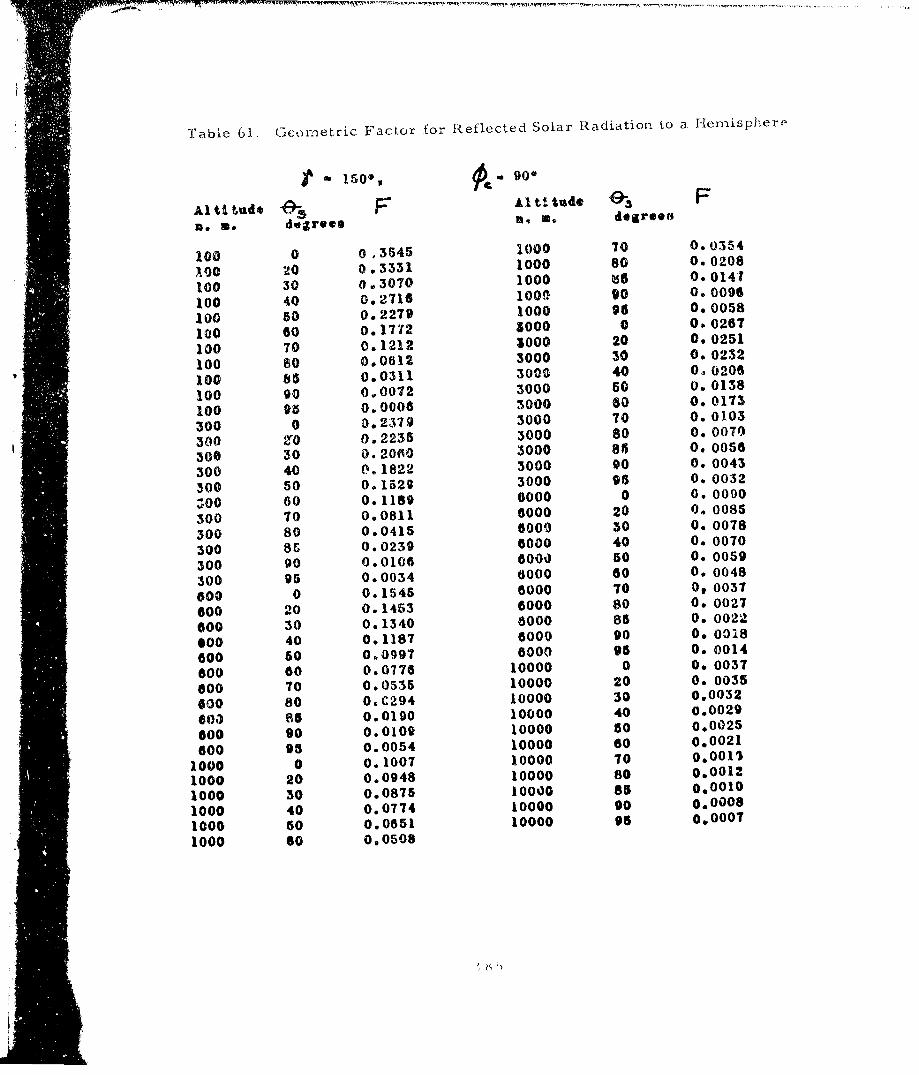
Table 61. Geomietric Factor for Reflected Solar Radiation to a Hemisphere

IO 150* ,- 90*

Ali0 udO e? F' Aitftud, * Fn.o . degrees ,. de~ree

100 0 0 3645 1000 70 0.0354

100 20 0.3331 1000 80 0.0208

100 30 0.3070 1000 b6 0.0141

100 40 0.2716 1000 90 0.0096

100 50 0.2279 1000 96 0.0058

100 60 0.1772 3000 0 0.0267

100 70 0.1212 3000 20 0. 0251

100 80 0.0612 3000 30 0.0232

100 85 0.0311 3000 40 00206

100 90 0.0072 3000 50 0,0138

100 93 0.0006 3000 60 0. 0173

300 0 0.2379 3000 70 0. 0103

300 410 0.2235 3000 80 0. 0079

300 30 0.2060 3000 8a 0. 0056

300 40 0.1822 3000 90 0. 0043

300 50 0.1529 3000 95 0. 0032

Z00 60 0.1189 6000 0 0. 0090

300 70 0.0811 6000 20 0, 0085

300 80 0.0415 6000 30 0. 0078

300 8B 0.0239 6000 40 0. 0070

300 90 0.0106 600%) 50 0. 0059

300 95 0.0034 8000 60 O. 0048

800 0 0.1545 8000 70 0, 0037

600 20 0.1453 6000 80 O. 0027

600 30 0.1340 8000 85 0. 0022

000 40 0.1187 6000 90 0. 0018

600 50 0.0997 6000 95 0. 0014

600 60 0.0776 10000 0 0. 0037

600 70 0.0535 10000 20 0. 0035

G00 80 0.C294 10000 30 0.0032

600 88 0.0190 10000 40 0.0029

000 90 0.0109 10000 50 0.0025

600 95 0.0054 10000 60 0.0021

1000 0 0.1007 10000 70 0.001s

1000 20 0.0948 10000 s0 0.0012

1000 30 0.0875 10000 85 0,0010

1000 40 0.0774 10000 g0 0,0008

1000 50 0.0651 10000 95 0.0007

1000 60 0.0508

mira

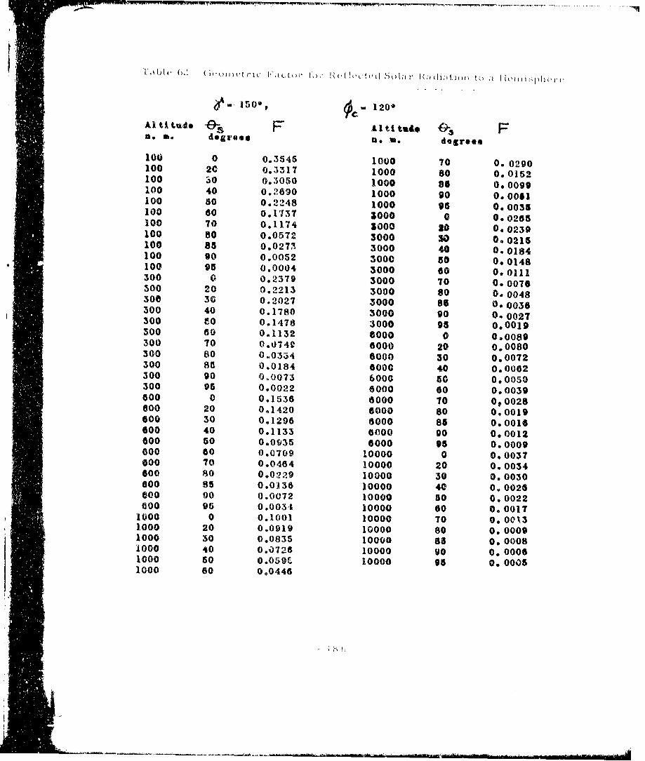
4~9' t)09 1200

Al tAtudo I £ti tudo &~12. a, degrees. u. we degrees100 0 0.3545 1000 70 0. 0290100 20 0.3317 1000 80 0.0152100 30 0.3050 1000 85 0,0099100 40 0.2890 1000 90 0.001100 50 0.2248 1000 95 0.0035100 60 0.1737 3000 0 0.0205100 70 0.1174 3000 20 0.0239100 80 0.0572 3000 30 0.0215100 85 0.0273 3000 40 0. 0184100 90 0.0052 3000 50 O. 0148100 95 0.0004 3000 00 0 0111300 0 0.2379 3000 70 0.0076300 20 0.2213 3000 80 0.0048300 30 0.2027 3000 85 0.0038300 40 0.1780 3000 90 0.0027300 cO 0.1478 3000 98 000019300 60 0.1132 6000 0 0.0089300 70 0.0749 60000 20 0.0080300 80 0.0354 6000 30 0.0072300 8 0.0184 8000 40 0,0002300 90 0.0073 6000 50 0.0050300 95 0.0022 8000 60 0.0039600 0 0.1536 8000 70 000028600 20 0.1420 6000 80 0.0019600 30 0.1296 8000 85 0.0016600 40 0.1133 6000 90 0.0012800 50 0.0935 6000 95 0.0009000 00 0.0709 10000 0 0.0037800 70 0.0464 10000 20 0.0034600 80 0,0229 10000 30 0.0030600 85 0.0136 10000 40 0.0026600 90 0.0072 10000 50 0.0022600 96 0.0031 10000 00 0. 0017

1000 0 0.1001 10000 70 0.00131000 20 0.0919 10000 80 0. 00091000 s0 0.0835 10000 85 0. 00081000 40 0.0728 10000 90 0. 00061000 50 0.059F 10000 95 0. 00051000 60 000446

1"-t

i 1500 ISO150'

AliF~d A~ I VA t utdO (

A. a. tudr.o no w. degree *

00 0.3 5 45 1.000 70 0. 0244

100 20 0.3307 1000 80 0.0111

10 00.3035 1000 85 0,0085

100 40 0.611000 go 0.00.36

100 40 0.2225 1000 96 O01019

100 60 0.1712 3000 20 0.0230

100 70 0.1146 300 0 0,0202

100 80 0.0543 300030020

100 85 0,0245 3000 40 0.0168

100 go 0.0031 3000 50 0,0130

100 95 0.0003 3000 80 0. 0092

300 0 0.2379 3000 70 0.,0057

300 20 0.2190 3000 s0 0. 003!

300 30 0.2003 3000 86 0.0022

300 40 0.1748 3000 90 00 0015

300 so 0.1441 3000 95 0. 0010

300 60 0.1090 600 0 c 0. j0GG

Soo 70 0.0704 8000 20 C. C017

300 80 0.0309 6000 30 0~l 0067

300 85 0.0144 0000 40 0.0056

300 90 0.0048 0000 50 0. 0044

300 96 0.0014 8000 60 0,0032

600 0 0.)530 8006 TO 0,022

600 20 0,1398 0000 s0 0.0014

000 30 0.1265 8000 85 0. (010

600 40 0.1094 6000 90 000008

600 50 0.0891 8000 95 0.0006

800 80 O..0660 10000 C 0.l 0037

Goo 70 0.0412 10000 20 0. 0032

600 80 0.0181 10000 30 0. 0029

800 05 0.0095 10000 40 0. 0024

G00 90 0.0045 10000 50 0. 0019

600 95 0.0020 10000 80 0. 0015

1000 0 0.0997 10000 10 0. 0011

1000 20 0.0898 10000 80 0. 0007

1000 30 0.0807 10000 so 0. 0006

1000 40 0.0691 10000 9o 0. 0005

1000 50 0.0554 10000 95 0. 0003

1000 60 000401

S100 86 0n024

Tl:[ L)4 L ~ Rele 4AI ci~t ' rH!cct SoL r HlI-to to a

A I it,,de, Alti tude 0 F1. as degr.6u n0 1. degreos

100 0 0.3545 1000 70 0. 0221100 20 0.3304 1000 80 0. o00s100 30 0.3030 1000 86 0. 0052100 40 0.2064 1000 90 0. 0026100 80 0.2217 1000 96 0. 0013100 cO0 0,1702 3000 0 0- 028400 70 0.1136 3000 20 0. 0227100 80 0.0533 3000 30 0- 0197iO0 85 0.0235 3000 40 0.0162100 90 0.0031 3000 50 0.0123100 95 0.0002 3000 O0 0.0084300 0 0.2379 3000 70 0.0050300 20 0.2190 3000 80 0,0025300 30 0.1994 3000 85 0.0017300 40 0.1737 3000 90 0.0010300 50 0.1427 3000 t5 0. 0006300 60 0.1075 8000 b 0.0089300 70 0.0687 6000 20 0. 0076300 80 0.0292 6000 30 0. 0066300 66 0.0130 6000 40 3. 0054300 90 0.0039 6000 60 0.0042300 95 0.0011 6000 60 0.0030600 0 0.1528 6000 70 0,0020600 20 0.1388 6000 80 0.0012600 30 0.1254 6000 86 0.0009600 40 0.1081 6000 90 0.0306600 50 0.0875 C000 S5 0.0004600 80 0.0843 10000 0 0.0007000 70 0.0394 10000 20 0. 0032600 80 010163 10000 30 0. 0028600 86 010081 10000 40 0. 0023600 90 0.0035 10000 50 Ol 0019600 95 0.0015 10000 80 0.0014

1000 0 0.099e 10000 70 0. 00101000 20 0.0891 10000 80 O. 00061000 30 0,079? 10000 85 0. 00051000 40 0.0678 10000 90 0.00041000 50 0.0539 10000 06 0. 00031000 60 0,0385

0')~,I .(,-o l'ot lt CtV SoIl, ca ( idton to it IvIl Ifli~phe ic

•- 180", •-. 0 -340"

&I ti tude F Altit a. O'd Fn. so degrees n. U. degrees

100 c 0.2907 1000 70 0.0022L

100 20 0.2731 1000 80 0.0134

100 30 0.2517 1000 88 0.0098

100 40 3.22226 1000 90 0.0067

100 50 0.1868 1000 95 0.0042

100 Go 0.1453 3000 0 0.0098

100 70 0.0994 3000 20 0.0093100 80 0.0501 3000 30 0.0085

100 85 0.0256 3000 40 0.0076

100 90 0.0064 3000 50 0.0064

100 95 0.0006 3000 60 010052

300 0 0.1815 3000 70 0.0039

300 20 0.1705 3000 so 0.0028

300 30 0.1571 3000 85 0.0024

300 40 0.!3i)0 3000 90 0.0019

300 50 01166 3000 95 0.0015

300 60 0.0907 6000 0 0.0017

300 70 0,0619 6000 20 0.0016

300 80 0.0316 6000 30 0.0015

300 85 0.0187 8000 40 0.0013

300 90 0.0089 6000 50 0.0011

30C 95 0.0030 6000 60 0.0009

600 0 0.1073 6000 70 0,0008

600 20 0.1009 6000 80 0.0006

600 50 0.0931 6000 85 0.0005

600 40 0.0824 6000 90 0,0004

800 50 0.0692 8000 95 0.0003

800 80 0.0539 10000 0 0.0003

600 70 0.0373 10000 20 0.0003

600 80 0.0208 10000 30 0.0003

800 85 0.0139 10000 40 0. 0002

Goo 90 0.0084 10000 50 0.0002

800 95 0.0044 10000 60 0 0002

1000 0 0.0625 10000 70 0. 0001

1000 20 0.0588 10000 80 0 o0001

ooo 30 0.0542 10000 85 0.0001

1000 40 0.0480 10000 90 0. 0001

1000 50 0.0403 10000 8 0. 0001

1000 60 0A316

FUig r 8, (. l puwic y for lPhnn..tary ReflectedI Sol;--i RIdaidtiofl to ;I Ji1lt Plate

qGeometric Factor, F

F FLAT PLATE

AREA, P -

tIORMAd'

SUN

-C

STable 66. Geometric FVactor for RIftcected Solar ladiatlion tio a t.'() lt at'

Altitude F Altitude 9- F

n. a. degree no n. degree

/104 0 0.9531 3000 0 0.2549100 20 0.8956 3000 20 0.2395100 30 0.8254 3000 30 0.2207100 40 0.7301 3000 40 0.1944100 50 0.6126 3000 50 0.1625100 60 0.4765 3000 60 0.1278100 70 0.3259 3000 70 0.0934100 80 0.1645 3000 80 0.0619100 85 0.0823 3000 85 0.0480100 90 0.0112 3000 go 0.0359300 0 0.8422 6000 0 0.1,102300 20 0.7914 6000 20 0.1036300 30 0.7294 6000 30 0.0950300 40 0.6452 6000 40 0.0837300 50 0.5414 6000 50 0.0708300 60 0.4211 6000 60 0.0573300 70 0.2874 6000 70 0.0440300 80 0.1459 6000 80 0.031C300 85 0.0777 6000 85 0.0260300 90 0.0253 6000 90 0.0209600 0 0.7121 10000 0 0.0514600 20 0.6691 10000 20 0.0482600 30 0.6167 10000 30 0.0442600 40 0.5455 10000 40 0.0391600 50 0.4577 10000 50 0.0335600 60 0.3557 10000 60 0.0276600 70 0.2423 10000 70 0.0218600 80 0.1271 10000 80 0.0163600 85 0.0160 10000 85 0.0138600 90 0.0367 10000 90 0.0114

1000 3 0.5792 20000 0 0.01581000 20 0.5443 20000 20 0.01481000 30 0.5016 20000 30 0.01361000 40 0.4437 20000 40 0.01211000 50 0.3723 20000 50 0.01051000 60 0.2882 20000 60 0.00891000 70 0.1976 20000 70 0.00721000 80 0.1102 20000 80 0.00561000 85 0.0728 20000 85 0.00481000 90 0.0429 20000 go 0.0041

!: (i

kI i

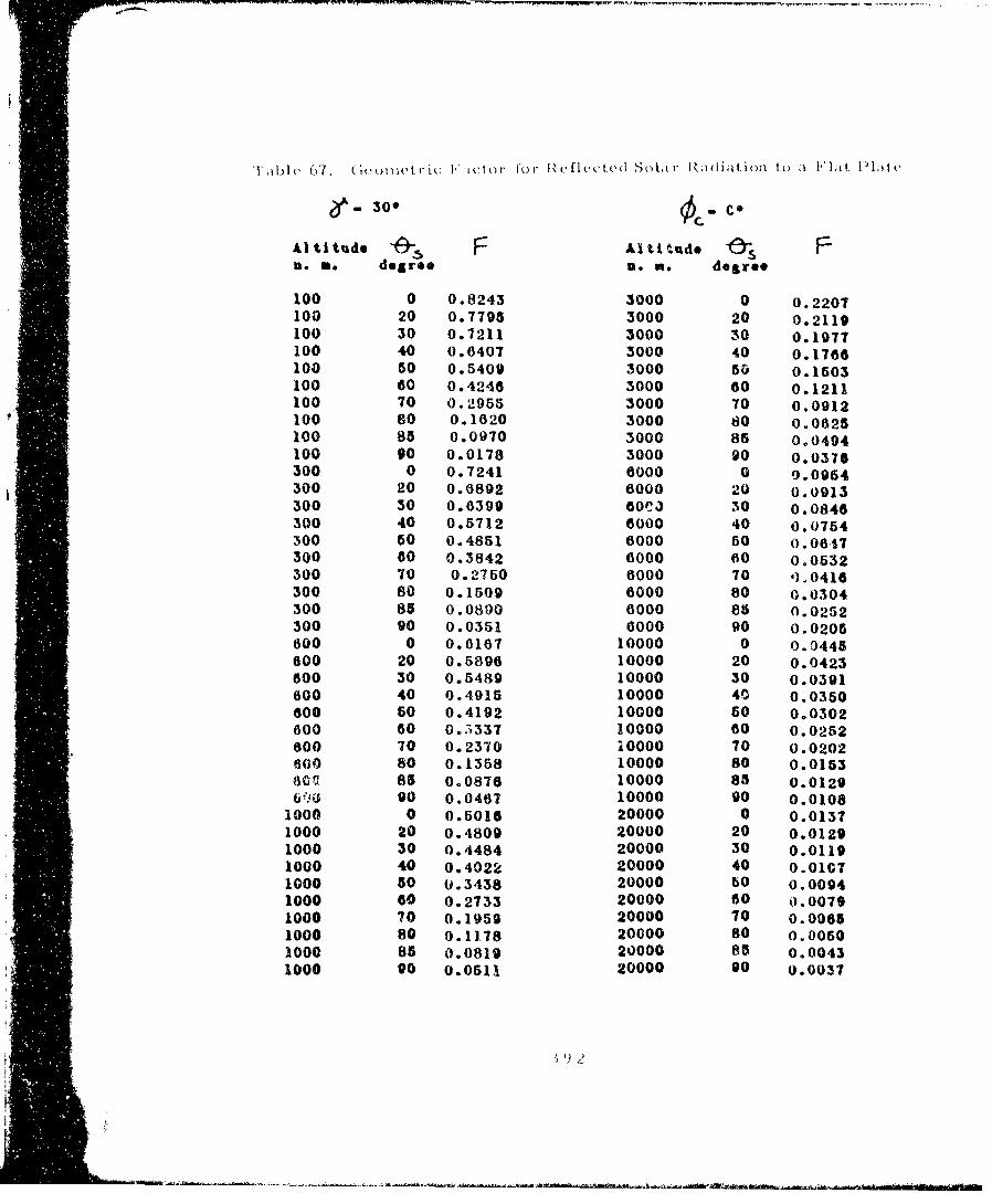
ialble 07. (Geuniet• ic' "•ctov f)or F'fl•ccted S(ltJ r l i.altioiin to a l'lat ,ldltke

e - 30" c-.e

Al ti tude (qs F Al titude 6s f=u. w. degree n. m. degree

100 0 0.8243 3000 0 0.2207100 20 0.7795 3000 20 0.2119100 30 0.7211 3000 30 0.1977100 40 0.6407 3000 40 0.1766100 50 0.5409 3000 50 0.1503100 60 0.4246 3000 60 0.1211100 70 0.2955 3000 70 0.0912100 80 0.1620 3000 80 0.0625100 85 0.0970 3000 85 0.0494100 00 0.0178 3000 90 0.0376300 0 0.7241 6000 0 0.0954300 20 0.6892 8000 20 0.0913300 30 0.6399 60CJ 30 0.0846300 40 0.5712 6000 40 0.0754300 50 0.4851 6000 50 0.0617300 60 0.3842 6000 60 0.0532300 70 0.2750 6000 70 0,0416300 80 0.1509 6000 80 0.0304300 85 0.0890 6000 so 0.0252300 90 0.0351 0000 90 0.0205600 0 0.6167 10000 0 0.0445600 20 0.5896 10000 20 0.0423600 30 0.5489 10000 30 0.0391600 40 0.4915 10000 40 0.0350600 50 0.4192 10000 60 0.0302600 60 0.5337 10000 60 0.0252600 70 0.2370 10000 70 0.0202600 80 0.1358 10000 80 0.0153Sc 85 0.0876 10000 83 0.0129V'0go 0.0467 10000 go 0.0108

1000 0 0.5016 20000 0 0.01371000 20 0.4809 20000 20 0.01291000 30 0.4484 20000 30 0.01191000 40 0.4022 20000 40 0.01o71000 50 0.3438 20000 60 0.00941000 60 0.2733 20000 60 0.00791000 70 0.1959 20000 70 0.00651000 80 0.1178 20000 80 0.00501000 85 0.0819 20000 83 0.00431000 90 0.0511 20000 90 0.0037

,TabLe .S (i. o rm .tric F actor to tI' 'l ctud Sola r t .nIdi atio!) t(o a L)t P tate

! ~'~ - 30" 0300~ 300

Altitude -es F Al ti tude '&.'s0. w. degree 0, N. dogrie

100 0 0.8243 3000 0 0.220?100 20 0.7788 3000 20 0.2113100 30 0.7201 3000 30 0.1908100 40 G.6395 3000 40 0.1755100 50 0.5394 3000 50 0.1490100 60 0.4230 3000 80 0.117100 70 0.2937 3000 70 0.0898100 80 0.1564 3000 80 '1.0613100 85 0.0841 3000 85 U.0483100 90 0.0167 3000 90 0.0367300 0 0.7241 6000 0 0.0954300 20 0.6880 8000 20 0.0911300 50 0.6382 0000 30 0.0843300 40 0.5690 6000 40 0.0750300 50 0.4824 8000 60 0.0042300 60 0.3813 0000 o0 !.0527300 70 0.2680 6000 70 0.0411300 80 0.1476 6000 80 0.0330300 85 0.0861 6000 85 0.0249300 go 0.0334 6000 90 0.0201600 0 0.6167 10000 0 0.0445000 20 0.5883 10000 20 0.0422600 30 0.5469 10000 30 0.0390800 40 0.4889 10000 40 0.0348600 50 0.4161 10000 60 0.0301600 60 0.3303 10000 60 0.0251600 70 0.2334 10000 70 0.0200600 80 0.1323 10000 80 0.0151600 85 0.0847 10000 85 0.0128o00 90 0.0447 10000 90 0.0107

1000 0 0.5016 20000 0 0.01371000 20 0.4796 20000 20 0.01291000 30 0.4165 20000 30 0.01191000 40 0.3998 20000 40 0.01071000 60 0.3409 20000 50 0.00931000 60 0.2702 20000 60 0.00791000 70 0.1925 20000 70 0.00641000 80 0.1148 20000 80 (t.0050"1000 88 0.0794 20000 85 0.00431000 90 0.0492 20000 90 0.0037

i;4

I,

0 - P0 5.- 606

AI ti tude F Al ti tudE F. N dear~o U. s, degr**

100 0 0.8k43 3000 0 0.2207100 20 0.7770 3000 20 0.2097100 30 0.7175 Z000 30 0.1944100 40 0.6361 3000 40 0.1725100 50 0.5354 3000 50 0.1455100 60 0.4184 3000 60 0.1159100 70 0.2887 3000 70 0.0860too 80 0.1455 3000 80 0.0581100 85 0.0790 3000 85 0.0455100 00 0.0137 3000 90 0.0343300 0 0.7241 6000 0 0.0954300 20 0.6848 6000 20 0.0905300 30 0.6335 6000 30 0.08S4

300 40 0.5629 6000 40 0.0740300 50 0.4752 8000 50 0.0630300 no 0.5731 6000 60 0,10514300 70 0.2595 6000 70 0.0396

300 80 0.1380 6000 80 0.0289300 85 0.0778 6000 85 0.0239500 go 0.0285 6000 90 0.0193600 0 0.6167 10000 0 0.0445

800 e0 0.5846 10000 20 0.0420

600 ;3 0.5415 10000 30 0.0387

600 40 0.4812 10000 40 0.0344

600 50 0.4078 10000 60 0.02966U) 60 0.3209 10000 00 0.0246

600 70 0.2234 10000 70 0.0195600 80 0.1229 10000 80 0.01.47

600 8g 0.0767 10000 85 0.012A600 90 0.0392 10000 90 0.0103

1000 0 0.5016 20000 0 0.0137

1000 20 0.4761 20000 20 0.0129

1000 30 0.4414 20000 30 0.0119

1000 40 0.3932 20000 40 0.0106

1000 50 0.3331 20000 60 0.0002

1000 60 0.2315 20000 60 0.0078

1000 70 0.1835 20000 70 0.0063

1000 80 0.1068 20000 80 0.0049

1000 85 0.0725 20000 85 0.0042

1000 90 0.0441 20000 90 0.0036

1! :

'I'able 70. Geon metri c Factor tor R~eflected Solar Racliatio) to a Flat P lzltc,

e~ - ooQ - 9006

Altitude 9 F Al ti tude e% Fn... degree m. m. degree

100 0 0.8243 3000 0 0.2207100 20 0.7746 3000 20 0.2074100 30 0.7138 3000 30 0A912100 40 0.6314 3000 40 0.1683100 50 0.5208 3000 50 0.1407100 60 0.4121 3000 60 0.1107100 70 0.2819 3000 70 0.0809100 80 0.1430 3000 80 0.0530100 85 0.0721 3000 85 0.0416100 90 0.0090 3000 90 0.0310300 0 0.7241 8000 0 0.0054300 20 0.6804 6000 20 0.0897300 30 0.6271 6000 30 0.0823300 40 0.6547 0000 40 0.0725300 50 0.4664 6000 50 0.0613300 60 0.3620 13000 60 0.0496300 70 0.2475 6000 70 00381300 80 0.1268 6000 80 0-0274300 85 0.0671 6000 85 V.-0225300 90 0.0217 6000 90 0.0181600 0 0.6167 10000 0 0.0445600 20 0.5795 10000 20 0.0417800 30 0.5340 10000 30 0.0383600 40 0.4724 10000 40 0.0339600 60 0.3964 10000 50 0.0290600 60 0.3081 10000 60 0,0239600 70 0.2098 1C0000 70 0.0189800 80 0.1101 10000 80 0.0141600 85 0.0668 10000 85 0.0119600 90 0.0318 10000 90 0.0099

1000 0 0.5016 20000 0 0.01371000 20 0.4714 20000 20 0.01281000 30 0.4344 20000 30 0.01181000 40 0.3843 20000 40 0.01051004 50 0.3224 20000 50 0.00911000 60 0.2496 20000 80 0.00771000 70 0.1711 20000 70 0.00621000 80 0.0954 20000 80 0.00481000 85 0.(,631 20000 85 0.00411000 90 0.0371 20000 90 0.0035

q

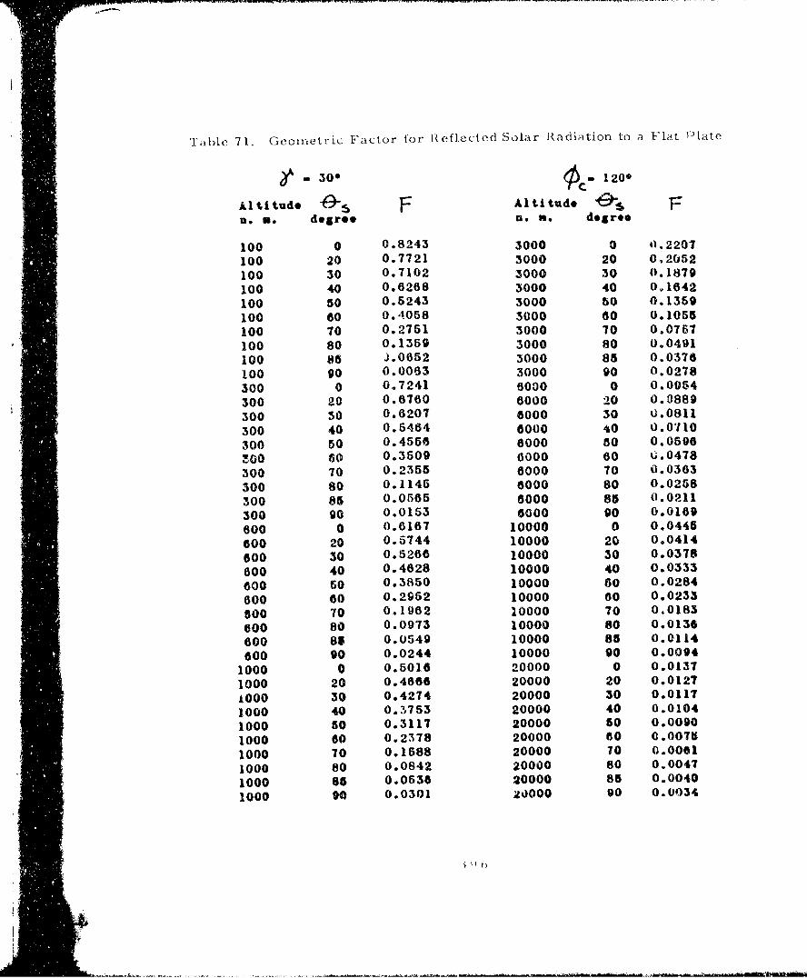
Tabic 7 1. Gcoinetric Factor for Reflected Solar Radiation to a Flat Plate

S- 30- 120

Altitud F Altitude Fn.o . degree n. n. degree

100 0 0.8243 3000 0 0.2207100 20 0.7721 3000 20 0,2052100 30 0.7102 3000 30 0.1879100 40 0.6268 3000 40 0.1642100 50 0.5243 3000 50 0.1359100 60 0.4058 3000 60 0.1055100 70 0.2751 3000 70 0.0757100 80 0.1359 3000 80 0.0491100 85 J.0652 3000 85 0.0376100 90 0.0063 3000 90 0.0278

300 0 0.7241 6000 0 0.0054300 20 0.6760 6000 20 0.0889

300 30 0.6207 6000 30 0.0811

300 40 0.5464 6000 40 0.0110

300 50 0.4556 8000 50 0.0569100 60 0.3509 6000 60 u.0478

300 70 0.2355 6000 70 0.0363

300 80 0.1145 6000 80 0.0258

300 85 0.0565 6000 85 0.0211

300 90 0.0153 6000 90 0.0169

600 0 0.6167 10000 0 0.0445

600 20 0.5744 10000 20 0.0414

600 30 0.5266 10000 30 0.0378

600 40 0.4628 10000 40 0.0333

600 50 0.3850 10000 60 0.0284600 60 0.2952 10000 60 0.0233Soo 70 0.1962 10000 70 0.0183

Soo 80 0.0973 10000 80 0.0136600 85 0.0549 10000 85 0.0114800 90 0.0244 10000 90 0.0094

1000 0 0.5016 20000 0 0.0137

1000 20 0.4666 20000 20 0.0127

t0oo 30 0.4274 20000 30 0.0117

1000 40 0.3753 20000 40 0.0104

1000 50 0.3117 20000 50 0.0090

1000 60 0.2378 20000 60 C.0075

1000 70 0.1588 20000 '10 0.0061

1000 80 0.0842 20000 80 0.0047

1000 85 0.0536 20000 85 0.0040

1000 90 0.0301 20000 90 0.0034

Table 72. Geometric Factor for Reflected Soiar Radiation to z Flat PI~lte

30 150

Altitude 195 F Altitiudo O-n.o.. degree a.*. degree

100 0 0.8243 3000 0 0.2207

100 20 0.7703 3000 20 0.2036

100 so 0.7076 3000 30 0.1855

100 40 0.6234 3000 40 0.1612

100 50 0.5202 3000 50 0.1324

100 60 0.4013 3000 60 0.1016

100 70 0.2701 3000 70 0.0719

100 80 0.1307 SUOO 80 0.0458

100 85 0.0603 3000 85 0.0348

100 90 0.0039 3000 90 0.0254

300 0 0.7241 eo0o 0 0.0954

300 20 0.6728 6000 20 0.0883

300 50 0.6160 5000 30 0.0802

300 40 0.5404 6000 40 0.0699

300 50 0.4484 8000 50 0.0583

300 o0 0.3428 6000 60 0.0465

300 70 0.2267 0000 70 0.0350

300 80 0.1056 8000 80 0.0247

300 88 0.0488 6000 85 0.0201

300 go 0.0107 6000 90 0.0160

600 0 0.6167 10000 0 0.0445

600 20 0.5707 10000 20 0.0412

600 30 0.5212 10000 30 0,0375

600 40 0.4558 10000 40 0.0329

600 50 0.3706 10000 50 0.0279600 60 j.2858 10000 60 0.0228

600 70 0.1863 10000 70 0.0178

600 8e 0.0879 10000 80 0.0132

600 85 0.0470 10000 88 0.0111

800 90 0.0189 10000 90 0.0091

1000 0 0.5016 20000 0 0.0137

1000 20 0.4631 20000 20 0.0127

1000 30 0.4223 20000 30 0.01161000 40 0.3687 20000 40 0.0103

1000 s0 0.3039 20000 60 0.0089

1000 60 0.2291 20000 60 0.0075

1000 70 0.1497 20000 70 0.0080

1000 80 0.0761 20000 80 0.0046

1000 85 0.0467 20000 85 0.00401000 90 0.0250 20000 90 0.0034

-- . .. . . -

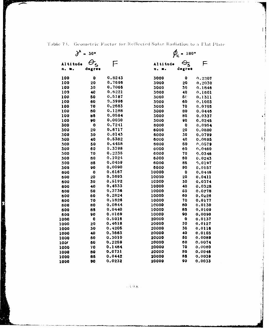
Ta'ble' 73. Gtcomletric t"itCtorI [*()I RtfCt'lCtd Solil- 1\';dialti, o1 tL) A I'lilt !Pltt(,

a 0- -180

Al ti tude FAl titude Fn. u. degree n. m. degree

100 0 0.8243 3000 0 0.2207100 20 0.7696 3000 20 0.2030100 30 0.7066 3000 30 0.1846100 40 0,6221 3000 40 0.1601100 50 0.518T 3000 56 0.1311100 60 0.3996 3000 60 0.1003100 70 0.2683 3000 70 0,0705100 80 0.1288 3000 80 0.0446100 85 0.0584 3000 86 0.0337100 90 0.0030 3000 go 0.0245300 0 0.7241 6000 0 0.0954300 20 0.6717 6000 20 0.0880300 50 0.6143 6000 30 0.0799300 40 0.5382 6000 40 0.0695300 50 0.4458 6000 60 A.0579300 00 0.3398 0000 60 0.0400300 70 0.2235 0000 70 0.0346300 80 0.1024 6000 80 0.0243300 88 0.0459 6000 85 1.0197300 90 0.0090 0000 90 0.0157600 0 0.6167 10000 0 0.0445600 20 0.5693 10000 20 0.0411600 30 0.5192 10000 30 0.0374600 40 0.4533 10000 40 0.0328600 50 0.3736 10000 60 0.0278600 60 0.2824 10000 60 0.0;26600 70 0.1828 10000 70 0.0177800 80 0.0844 10000 80 0.0130600 85 0.0440 10000 85 0.0109600 90 010169 10000 90 0.0090

1000 0 0.5016 20000 0 0.01371000 20 0.4618 20000 20 0.01271000 30 0.4205 20000 30 0.01161000 40 0.3883 20000 40 0.01031000 50 0.3010 20000 60 0.0089100( 60 0.2259 20000 60 0.00741000 70 0.1464 20000 70 0.00601000 80 0.0731 20000 80 0.00461000 865 0.0442 20000 85 0.00391000 90 0.0232 20000 90 0.0033

IR~

-60. 0'

Al ti tudoe e F tude FD. A. degree U. No degree

100 0 0.6004 3000 0 0.1260100 20 0.5708 3000 20 0.1250

100 30 0.5296 3000 30 0.1201100 40 0.4723 3000 40 0.1116100 50 0.4008 3000 50 0.09V2100 60 0.3168 3000 80 0.0820100 70 0.2234 3000 70 0.0646100 80 0.1220 3000 80 0.0464100 85 0.0079 3000 85 0,0375100 00 0.0198 3000 90 0.0292300 0 0.4905 8000 0 0.0551300 20 0.4727 8000 20 0.0546300 30 0.4420 6000 30 (1.0510300 40 0.3979 8000 40 0.0470300 50 0.3417 6000 50 0.0413300 80 0.2751 6000 60 0.0349300 70 0.3000 0000 70 0.0281300 80 0.1170 6000 80 0.0211300 85 0.0760 0000 85 0.0177300 90 0.0355 0000 90 0.0146600 0 0.3889 10000 0 0.0257G00 20 0,3798 10000 20 0.0251600 30 0.3577 10000 30 0.0236800 40 0.3248 10000 40 0.0214800 60 0.2821 10000 60 0.0189000 60 0.2334 10000 80 0.0160800 70 0.1075 10000 70 0.0131600 80 0.1050 10000 80 0.0101600 85 0.0768 10000 85 0.0086600 90 0.0441 10000 90 0.0072

1000 0 0.5011 20000 0 0.00791000 20 0.2979 20000 20 0.00761000 30 0.2823 20000 30 0.00711000 40 0.2582 20000 40 0.00641000 50 0.2262 20000 s0 0.00571000 60 0.1885 20000 60 0,00481000 70 0.1390 20000 70 0.00401000 80 0.0938 20000 80 0.003".1000 805 0.0691 20000 85 0.00271000 g0 0.0456 20000 90 0.0023

"I IIII

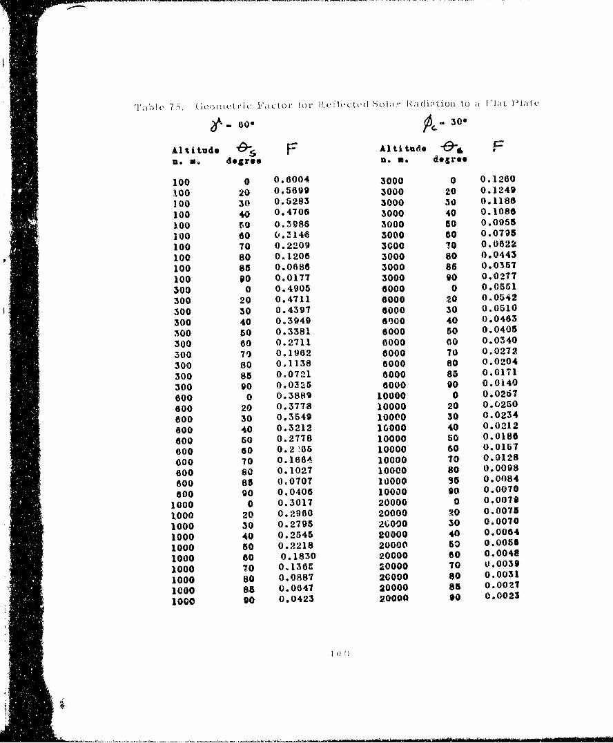
1:1 7 5, G()oI IIet ric Iitct. to I or R,(!'to hctt)(1 S' oa rIa ldi;,Lion to a IL~tt P i t t

e - - 30

Al t itude 6)S F AltUitude -,6 Fn.o . degree n.o . degree

100 0 0.6004 3000 0 0.1260

X00 20 0.5699 3000 20 0.1249

100 30 0.5283 3000 30 0.1186

100 40 0.4706 3000 40 0.1086

100 C0 0.3986 3000 s0 0.0955

100 60 0.3146 3000 60 0.0725

100 70 0.2209 3000 70 0.0622

100 80 0.1206 3000 80 0.0443

100 85 0.0686 3000 85 0.0357

100 90 0.0177 3000 90 0.0217

300 0 0.4905 6000 0 0.0551

300 20 0.4711 8000 20 0.0542300 30 0.4397 6000 30 0.0510

300 40 0.3949 63000 40 0.0463

300 50 0.3381 6000 50 0.0405

300 60 0.2711 6000 00 0.0340

300 70 0.1962 6000 70 0.0272

300 80 0.1138 6000 80 0.0204

300 85 0.0721 6000 85 0.0171

300 90 0.0325 6000 90 0.0140

600 0 0.3889 10000 0 0.0267

600 20 0.3778 10000 20 0.0250

600 30 0.3549 I0000 30 0.0234

600 40 0.3212 10000 40 0.0212

600 50 0.2778 10000 60 0.0188

o00 60 0.2'05 10000 60 0.0157

000 70 0.1664 10000 70 0.0128

600 80 0.1027 10000 80 0.0098

600 85 0.0707 10000 35 0.0084

o00 90 0.0406 10000 g0 0.0070

1000 0 0.3017 20000 0 0.0079

1000 20 0.2960 20000 P0 0.0075

1000 30 0.2795 20000 30 0.0070

1000 40 0.2545 20000 40 0.0064

1000 50 0.2218 20000 50 0.0056

1000 60 0.1830 20000 60 0.0048

1000 70 0.136E 20000 70 0.0039

1000 80 0.0887 20000 80 0.0031

1000 85 0.0647 20000 85 0.0027

1000 90 0.0423 20000 90 0.0023

Table 76. Geonnetric Factor lor B. ,flcted Solar Radiation to a Flat P lat I

60 600

Altitude Altitud.

n.m. degree *.. degree

100 0 0.6004 3000 0 0.1260

100 20 0.5675 3000 20 0.1222

100 30 0.5248 3000 30 0.146

100 40 0.4661 3000 40 0.1035

100 50 0.3933 3000 50 0.0895

100 60 0.3085 3000 60 0.0727

"100 70 0.2143 3000 70 0.0556

"100 80 0.1136 3000 80 0.0387

100 83 0.0616 3000 85 01,0307

100 so 0.0134 3000 90 0.0236

300 0 0.490 O00NG 0 0.6551

"300 20 0.4668 8000 20 0.05•2

300 50 0.4334 6000 30 0.0495

300 40 0.3868 6000 40 0.0444

300 50 0.3285 6000 50 0.0383

300 G0 0.2002 6000 60 0.031?

300 70 0.1837 6000 70 0.0250

300o 80 0.1015 6000 80 0.0184

300 85 0.0oo6 6000 85 0.0153

300 90 0.0252 6000 g0 0.0125

800 0 0.3889 10000 0 0.0257

800 20 0.3726 10000 20 0.0246

600 30 0.3472 I0000 30 0.0228

600 40 0.3114 10000 40 0.0205

600 50 0.2600 10000 60 0.0178

5300 60 0.2124 10000 60 0.0149

600 70 0.1518 10000 70 0.0120

o00 80 0.0886 10000 80 0.0091

600 85 0.0580 X0000 65 0.0077

600 90 0.0325 10000 90 0.0065

1000 0 0.3017 20000 0 0.0079

1000 20 0.2907 20000 20 0.0075

1000 30 0.2718 20000 30 0.0069

1000 40 0.2446 20000 40 0.0062

1000 50 0.2100 20000 50 0.0054

1000 60 0.1700 20000 60 0.00A6

1000 70 0,1224 20000 70 0.0038

1000 80 0.0754 20000 80 0.0029

1000 88 0.0529 20000 85 0.0025

1000 90 0.0345 20000 90 0.0022

T'iblc 77. Geornetric Factor for I '. Ii.t I SoLlt I Radiation to a FlI t IPij)aiLc

Al tItude 4 F Altitude GI Fn. f. degree fo Ws degree

100 0 0.6004 3000 0 0.1260100 20 0.5642 3000 20 0.1184100 30 0.5200 3000 30 0.1091100 44) 04599 3000 40 0.0964100 50 0.384t 3000 s0 0.0812100 60 0.3002 3000 66 0.0637100 70 0.2053 3000 70 0.0464100 80 0.1042 3000 60 0.OS06100 85 0.0525 3000 83 0.0215100 00 0.0078 3000 00 0.0175300 0 0.4905 8000 0 0.0551300 20 0.4609 6000 20 0.0b18300 30 0.4248 6000 30 0.0475300 40 0.3757 6000 40 0.0418300 50 0,3153 6000 50 0.0354300 62 0.%452 6000 60 0.0286300 70 0.1678 1000 70 0.1220300 80 0.0852 6600 8W 0.0158300 85 0.0,159 6000 8a 0.0150300 40 0.0148 Ocoo go 0.0104600 0 0.3889 10000 0 0.0257600 20 0.3654 10000 20 1.0241600 30 0.3368 I000o 30 0.0221o00 40 0,2972 10000 40 0.0193

600 50 0.2499 13000 so 3.0A67600 60 0.1943 10000 00 0.0038600 70 (,13125 10000 7U 0.0109

o600 80 0.0700 10000 0 0.0081600 85 0.0420 10000 86 0.0069600 90 0.0198 10000 90 0.0957

1000 0 0.3017 20001 0 0.00791000 20 0.21835 20000 20 0.00741000 30 0.2613 20000 30 0.00681000 40 0.2311 20000 40 3.00601000 60 011939 20000 60 0.00521000 5O 0.i503 20000 60 0.C0441000 70 0.1035 20000 70 0.00361000 80 0.0580 20000 60 0.00201000 85 0.0381 20000 85 0,00241000 O0 0.0222 21000 90 0.0020

-4 0

F.'T 7 . G eo met i c l'cto ' for I Qf ,ted )1o8ld r G ,ai tio l I to 1 1 ; P la tt ,

6-00 o-120"'

PA#,i tude Al ti tde 19ZI. F. degree n.m. degroe

100 0 0.6004 3000 0 0.1263

100 20 0.5009 3000 20 0.1140

100 30 6.5152 3000 30 0.1036

100 40 0.4638 3000 40 0.0894

100 50 0.3786 3000 s0 0.0729

100 30 0.2919 3000 00 0.0548

100 7C 0.1963 3000 70 0.0378

100 80 0.0948 3000 80 0.0230

100 88 0.0435 3000 85 0.0170

100 90 0o.052 3000 90 0.0121

300 0 0.4005 6000 0 0.0551300 20 0.4550 6000 20 0.0503

300) 50 0.4162 6000 30 0.0464

300 40 0.304' 6000 40 0.0393

300 50 0.3021 6000 50 0.0324300 60 0.2303 8000 60 0.0255300 TO 0.1514 5000 70 0.0189300 80 0.0893 6000 80 0.0131300 85 0.0320 6000 85 0.0106

300 90 0.0074 6000 go 0.0083

600 0 0.3880 10000 0 0.0257

800 20 0.3582 10000 20 0.0235

600 30 0.3263 10000 30 0.0215

800 40 0.2844 10000 40 0.0186

800 60 0.2339 10000 50 0.0167

800 60 0.1762 10000 60 0.0127

600 70 0.1132 10000 70 0.0098600 80 0.0521 10000 80 0.0072600 85 0.0271 10000 85 0.0060600 90 0.0105 1000( 90 0.0049

1000 0 0.3017 20000 0 0.00791000 20 0,2703 20000 20 0.0073

1000 30 0.2507 20000 30 0.0066

1000 40 0.2176 20000 40 0.00591000 60 0.1778 20000 50 0.0050

1000 80 0.1323 20000 60 0.0042

1000 70 0.0847 20000 70 0.0034

1000 80 0.0414 20000 80 0.0026

1000 85 0.0243 20000 85 0.00221000 90 0.0123 20000 90 0.0019

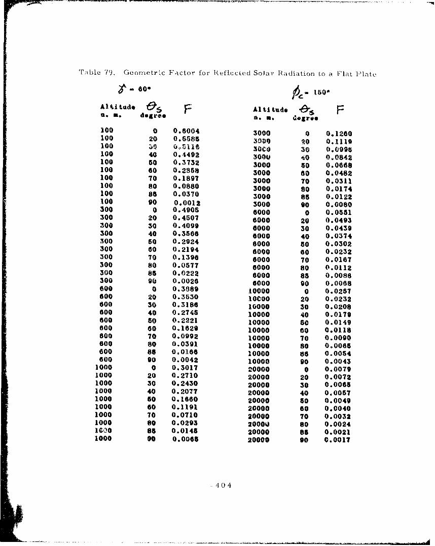
Table 79. Geomrnetric Factor for Reflected Solar Radiatiori to a Flat Plate

Y,- 80*A 01

Altitud S F Altitude Fn. so dgte*o no no degree

100 0 0.6004 3000 0 0.1260100 20 0.5585 3000 o0 0.1110100 r 0IsI16 30CO 30 0.0996100 40 0.4492 3000 i0 0.0842100 50 0.3732 3000 50 0.0668100 60 0.2358 3000 60 0.0482100 70 0.1897 3000 70 0.0311100 80 0.0880 3000 80 0.0174100 85 0.0370 3000 85 0.0122100 90 0.0012 3000 90 0.0080300 0 0.4905 6000 0 0.0551300 20 0.4507 6000 20 0.0493300 50 0.4099 6000 30 0.0439300 40 0.3566 6000 40 0.0374300 50 0.2924 6000 50 0.0302300 00 0.2194 6000 60 0.0232300 70 0.1396 6000 70 0.0167300 80 0.0577 6000 80 0.0112300 85 0.0222 6000 85 0.0088300 90 0.0020 6000 go 0.0068o00 0 0.3889 10000 0 0.0257

600 20 0.3530 0OCO0 20 0.0232600 30 0.3186 10000 30 0.0208600 40 0.2745 10000 40 0.0179600 50 0,2221 10000 s0 0.0149600 60 0.1629 10000 60 0.0118600 70 0.0992 10000 70 0.0090600 80 0.0391 10000 80 0.0065600 85 0.0166 10000 as 0.0054600 90 0.0042 10000 90 0.0043

1000 0 0.3017 20000 0 0.00791000 20 0.2710 20000 20 0.00721000 30 0.2430 20000 30 0.00651000 40 0.2077 20000 40 0.00571000 50 0.1660 20000 50 0.00491000 60 0.1191 20000 60 0.00401000 70 0.0710 20000 70 0.00321000 80 0.0293 20000 80 0.00241600 85 0.0145 20000 85 0.00211000 90 0.0065 20000 90 0.001?

-404

Table 80. Geometric Factor for N~eflected Solar Radiation to a Flat Plate

61 - 60" A - 180"

Altitude -5 F Altitude fZ'n. m. degree Ik m. degree

100 0 0.6004 3000 0 0.1268100 20 0.5576 3000 20 0,1108100 s0 0.51C4 3000 30 0.0981100 40 0.4476 3000 40 0.0823100 50 0.3712 3000 50 0.0648100 60 0.2836 3000 00 0.0458100 70 0.1873 3000 70 0.0287100 80 0.0855 3000 80 0.0154100 85 0.0347 3000 85 0.0104100 90 0.0003 3000 90 0.0088300 0 0.4905 6000 0 0.0551300 20 0.4491 6000 20 0.0489300 30 0.4076 0000 30 0.0434300 40 0.3536 6000 40 0.0367300 50 0.2889 8000 50 0.0295300 60 0.2154 8000 60 0.0223300 70 0.1363 6000 70 0.0159300 80 0.0534 6000 80 0.0105300 85 0.0187 6000 85 0.0082300 90 0.0010 6000 90 0.0062600 0 0.3889 10000 0 0.0257600 20 0,3511 10000 20 0.0230600 s0 0.3168 10000 30 0.0206600 40 0.2709 10000 40 0.0177600 50 0.2178 10000 60 0.0146600 s0 0.1581 10000 60 0.0115600 70 0.0940 10000 70 0.0087600 80 0.0344 10000 80 0.0082600 85 0.0128 10000 85 0.0051G00 90 0.0020 10000 90 0.0041

1000 0 0.3017 20000 0 0.00791000 20 0.2691 20000 20 0.00721000 30 0.2402 ?0000 30 0.00651000 40 0.2040 20000 40 0.00571000 50 0.1617 20000 50 0.00481000 60 0.1143 20000 80 0.00401000 70 0.0660 20000 70 0.00311000 8o 0.0249 20000 so 0.00241000 8N 0.0109 20000 85 0.00201000 90 0.0032 20000 90 0.0017

- 405

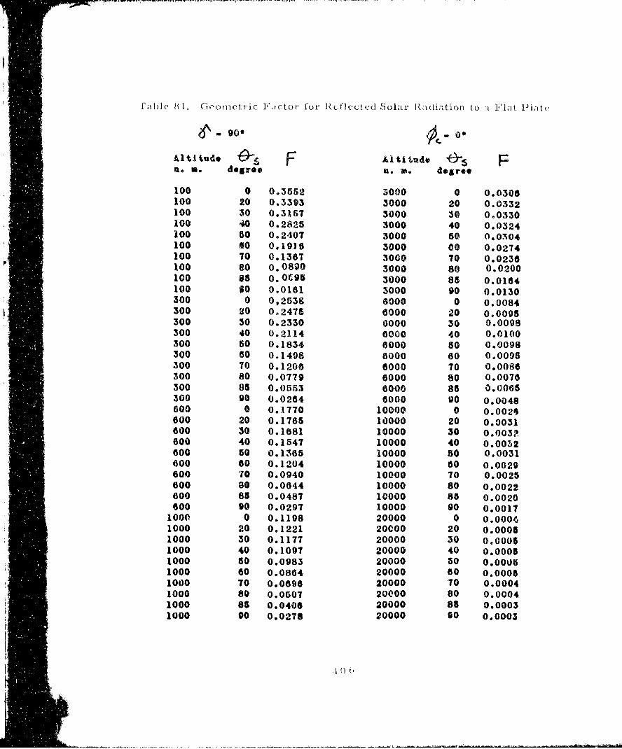
La Wc B t. (jeomel ic t'Ictor for Reflected Solar , diation to :I Fla( Plat1

4- 90' A I 0t

Altitude s F Al ti tude FO n.. degree no we degree

100 0 0.3552 300 0 0.0308100 20 0.3393 3000 20 0.0332100 30 0.3157 3000 30 0.0330100 40 0.2825 3000 40 0.0324100 50 0.2407 3000 50 0.0304100 00 0.1916 3000 00 0.0274100 70 0.1367 3000 70 0.0236100 80 0.0890 3000 80 0.0200100 85 O.OC95 3000 85 0.0164100 00 0.0161 3000 90 0.0130300 0 0,2538 6000 0 0.0084300 20 o O2475 6000 20 0.00o8300 30 0.2330 6000 30 0.0098300 40 0.2114 0000 40 0.0100300 50 0.1834 6000 80 0.0098300 60 0.1498 8000 60 0.0095300 70 0.1206 6000 70 0.0086300 80 0.0779 6000 80 0.0076300 85 0.0553 6000 85 0.0065300 90 0.0264 o000 go 0.0048000 0 0.1770 10000 0 0.002)600 20 0.1765 10000 20 0.0031600 30 0.1681 10000 30 0.003P600 40 0.1647 10000 40 0.0012600 60 0.1365 10000 50 0.0031600 60 0.1204 10000 60 0.0029600 70 0.0940 10000 70 0.0025600 80 0.0644 10000 80 0.0022800 85 0.0487 10000 86 0.0020600 90 0.0297 10000 90 0.0017

1000. 0 0.1198 20000 0 0.00041000 20 0,1221 20000 20 0.00051000 30 0.1177 20000 30 0M00051000 40 0.1097 20000 40 0.00051000 50 0.0983 20000 50 0.00051000 60 0.0864 20000 60 0.00051000 70 0.0696 20000 70 0.00041000 80 0.0507 20000 80 0.00041000 85 0.0408 20000 85 0.00031000 00 0.0278 20000 s0 0.0003

'1I () 0

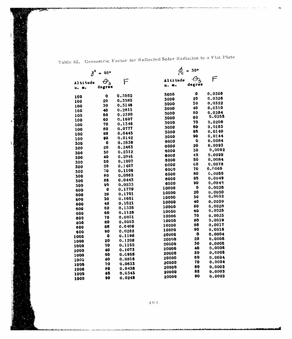
Table 8Z. GeoiettiC 1'actor eo -Refiected Sot r RadiaLrof to a c'lat IItt

9. 0" 0 30"

Al tit uds .&S Al ti tude Fn.*. degree U. A. degroe

100 0 0.3552 3000 0 0.0306

100 20 0.3385 3000 20 0.0326

100 30 0.3146 3000 30 0.0322

100 40 0.2811 3000 40 0.0310

100 50 0.2390 3000 50 0.0284

100 60 0.1897 3000 60 0.0255

lOG 70 0.1346 3000 70 0.0206

100 80 0.0777 3000 80 0.0183

100 B8 0.0443 3000 85 0.0140

100 90 0.0142 3000 90 0.0144

300 0 0.2538 6000 0 0.0084

300 20 0.2463 6000 20 0.0093

300 50 0.2312 6000 30 0,0092

300 40 0. 2 041 6000 40 0.0090

300 50 0.1807 5000 50 0.0084

300 30 0.1467 6000 00 0.0076

300 70 0.1105 6000 70 0.6065

300 80 0.0663 6000 80 0.0056

300 85 0.0443 6000 85 0.0049

300 90 0.0233 6000 90 0.0041

600 0 0.1770 10000 0 0.0026

600 20 0.1751 10000 20 0.0030

600 30 0.1661 10000 30 0.0032

600 40 0.1521 10000 40 0.0030

600 60 0.1335 10000 50 0.0028

600 60 0.1126 10000 60 0.0025

600 70 0.0851 10000 70 0.0023

600 80 0.0553 10000 80 0.0019

600 88 0.0406 10000 86 0.0017

600 90 0.0282 10000 90 0.0015

1000 0 0.1198 20000 0 0.0004

1000 20 0.1208 20000 20 0.0005

1000 30 0.115S 20000 30 0.0006

1000 40 0.1073 20000 40 0.0005

1000 50 0.C955 20000 s0 0.0005

100I 80 0.0816 20000 60 0.0004

1000 70 0.0633 20000 70 0.0004

1000 80 0.0438 20000 80 0.0003

1000 85 0.0343 20000 85 0.0003

1000 90 0.0245 20000 90 0.0003

-4 (J

T'able 83. Geonei ric F'actor for Reflected Solar Radiation to a Fla. t Plate

0 o0

Al ti trd* 4 F Al ti tudeFn. m. degree n. no dogree

100 0 0.3552 3000 0 0.0306100 20 0,3305 3000 20 0.0310100 30 0.3116 3000 30 0.02980oo 40 0.2773 3000 40 0.0275

loo 50 0.2345 3000 60 0.0243

100 60 0.1846 3000 63 0.0205100 70 0.1290 3000 70 0.0165

0oo 80 0.0090 30c0 80 0.0122100 85 0.0382 3000 85 0.0100100 g0 0.0098 3000 90 0.0079300 0 0.2538 8000 0 0.0084

V 300 20 0.2430 6000 20 0.0087300 50 0.2264 6000 30 0.0084o00 40 0.V)29 6000 40 0.0078

300 50 0.1732 6000 50 0.0070300 60 0.1383 6000 60 0.0060300 70 0.0992 6000 70 0.0051300 80 0.0564 0000 80 0.0040300 85 0.0352 6000 8s 0.0034300 go 0.0161 6000 90 0.0029600 0 0.1770 10000 0 0.0026

o00 20 0.1714 10000 20 0.0027600 30 C.1607 10000 30 0.0027600 40 0.1451 10000 40 0.0025600 50 0.1251 10000 50 0.0023800 60 0.1015 10000 60 0.0020000 70 0.0738 10000 70 0.0017600 80 0.0449 10000 80 0.0014600 89 0.0310 10000 85 0.0012600 90 0.0181 10000 90 0.0010

1000 0 0.1198 20000 0 0.000o1000 20 0.1173 20000 20 0.00041000 30 0.1107 20000 30 0.00041000 40 0.1007 20000 40 0.00041000 50 00877 20000 so 0.00041000 80 0.0715 20000 00 0.00031000 70 0.0532 20000 70 0.00031000 80 0.0346 20000 80 0.00021000 85 0.0255 20000 85 0.00021000 90 0.0189 20000 90 0.000a

t$

Table 84. Ge•ometric Factor foi Reflected Solar Radiation to a Flat Plate

* 90- 906

Altitude F Altitudw Fn.0 . degrer n. no degree

100 0 0.3552 3000 0 0.0306100 20 0.3337 3000 20 0.0288100 30 0.3076 3000 30 0.0265100 40 0.2721 3000 40 0.0233p.00 50 0.2283 3000 60 6.0194100 60 0.1776 3000 60 0.0162190 70 0.1214 3000 70 0.0111100 80 0.0008 3000 80 0.0073100 85 0.0305 3000 85 0.0066I00 90 0.0051 3000 90 0.0041300 0 0.2538 6000 0 0.0084300 20 0.2385 6000 20 0.0078300 ;s0 0.2198 6000 30 0.0072300 40 e.1944 6000 40 0.0063300 50 0.1631 6000 50 0.0053300 n0 0.1269 6000 60 0.0043300 70 0.0865 6000 70 0.0033300 00 0.0438 6000 80 0.0023300 85 0.0238 6000 85 0.0019300 90 0.0084 6000 90 0.0015600 0 0.1770 10000 0 0.0026600 20 0.1663 10000 20 0.0024800 30 0.1532 10000 30 0.0022600 40 0.1356 10000 40 0.00208G0 50 0.1137 10000 60 0.0017b00 60 0.0883 10000 60 0.0014G00 70 0,0599 10000 70 0.0011600 80 0.0316 10000 80 0.0008"8v0 b3 0.0191 10000 86 0.0006800 90 C.0094 1000C 90 0.0005

1000 0 3.1198 20000 0 0.00041000 24 G.1125 20000 20 0.00041000 3 V 0.1037 20000 30 0.00031000 40 0.0917 20000 40 0,00031000 s0 0.0770 20000 s0 0000031000 60 0,0593 20000 60 0.00021000 70 0.0408 20000 70 0.00021000 80 0.G227 20000 g0 0.000o1000 CS O.0A50 20600 8 0.00011000 90 0.0088 20000 90 0.9001

A ) 9

Table 85. Geometric Fictor for Reflected Solar R.zdiat~ou. to :i Flat Plate

ý, - 90g A- 120"

Altitude F Alt itude Os Fn. m. degree a.m. m egree

100 0 0.3652 3000 0 0.0306100 20 0.3510 3000 20 0.0265100 30 0.3035 3000 30 0.0232100 40 0.2669 3000 40 0.0191100 50 0.2221 3000 50 0.0148100 60 0.1706 3000 60 0.0101100 70 0.1138 3000 70 0.0082100 80 0.0529 3000 80 0.0032100 88 0.0230 3000 85 0.0022100 90 0.0017 3000 90 0.0014300 0 0.2538 6000 0 0.0084300 20 0.2339 6000 20 0.0070300 50 0.1132 6000 30 0.0060300 40 0.1859 6000 40 0.0048300 50 0.1530 6000 50 0.0036300 60 0.1154 6000 60 0.0024300 70 0.0742 6000 70 0.0016

300 80 0.0317 6000 80 0.0009300 86 0.0135 0000 85 0.0007

300 90 0.0028 8000 90 0.0005600 0 0.1770 10000 0 0.0026600 20 0.1612 10000 20 0.0022600 30 0.1458 10000 30 0.0018600 40 0.1260 10000 40 0.0014600 50 0.1023 10000 50 0.0011600 60 0.0755 10000 60 0.0008600 70 0.0464 10000 70 0.0005600 80 0.0193 10000 80 0.0003

600 85 0.0092 10000 85 0.0002600 90 0.0032 10000 90 0.0001

1000 0 0.1198 20000 0 0.00041000 20 0.1078 20000 20 0.00031000 30 0.0967 20000 30 0.00031000 40 0.0828 20000 40 0.00021000 50 0.0663 20000 50 0.00011000 60 0.0475 20000 60 0.00001000 70 0.0284 20000 70 0.00001000 80 0.0123 20000 80 0.00001000 85 0.0066 20000 85 0.00001000 90 0.0030 20000 90 0.0000

I I c

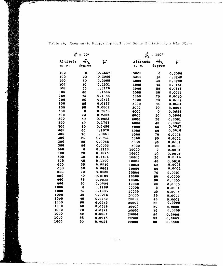
T abe 8 0. C eoinet ric t'actor for 'eflect:ed Solar Radiption to ;i Flat Plate

9- o00 A 1606

*Altitude FAl titude, KEn. we degroe S. .N degree

100 0 0.3552 3000 0 0.0306100 20 0.3290 3000 20 0.0249i0o 30 0.3006 3000 30 0.0209100 40 0.2631 3000 40 0.0161100 50 0.2175 3000 50 0.0111100 60 0.16854 3000 60 0.0065100 70 0.1083 3000 70 0.0030100 80 0.0471 3000 80 0.0009100 85 0,0177 3000 85 0.0004100 90 0.0002 3000 00 0.0001300 0 0.2538 6000 0 0.0084300 20 0.2306 6000 20 0.0064300 30 0.2083 6000 30 0.0051300 40 0.1797 6000 40 0.0037300 50 0.1456 8000 50 0.0027300 60 0.1070 6000 60 0.0016300 70 0.0651 6000 70 0.0006300 80 0.0231 6000 80 0.0002300 88 0.0068 6000 88 0.0001300 90 0.0003 6000 go 0.0000600 0 0.1770 10000 0 0.0026800 20 0.1675 10000 20 0.0019600 30 0.1404 10000 30 0.0014600 40 0.1190 10000 40 0.0010600 50 0.0940 10000 s0 0.0006600 60 0.0661 10000 60 0.0002600 70 0.0365 10000 70 0.0001600 80 0.0109 10000 80 0.0000600 88 0.0032 10000 85 0.0000600 90 0.0004 10000 90 0.0000

1000 0 0.1,98 20000 0 0.00041000 20 0.1043 20000 20 0.00031000 30 0.0918 20000 30 0.00021000 40 0.0,72 20000 40 0.00011000 60 0.0505 20000 50 0.00001000 60 0.0389 20000 80 0.00001000 70 0.0197 20000 70 0.00001000 80 0.0055 20000 80 0.00001000 88 0.001 2W0000 85 0.00001000 90 0,0004 20000 90 0.0000

!!! ¥- ~ ~ a& i&~

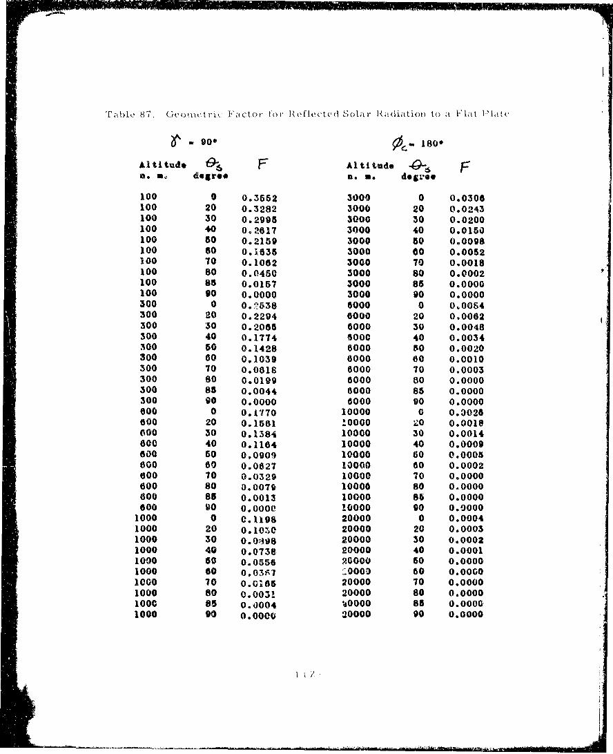
Table 87. Geomcft ric I' actor for RefectL't(d Sola r I/adiatioil to a ltFlat Ilatc

S- go. A-180"

Altitude t19- F Al ti tude -&-S Fa. no degreoe n.o. dng*ee

100 0 0.3552 3000 0 0.0306100 20 0.3282 3000 20 0.0243100 30 0.2995 3000 30 0.0200100 40 0.2817 3000 40 0.0150100 50 0.2159 3000 50 0.0098100 60 0.1835 3000 60 0.0052100 70 0.1062 3000 70 0.0018100 80 0.0450 3000 s0 0.0002100 85 0.0157 3000 85 0.0000100 00 0.0000 3000 90 0.0000300 0 0."638 6000 0 0,00S4300 20 0.2294 6000 20 0.0082300 30 0.2085 0000 30 0.0048300 40 0.1774 8000 40 0.0034300 50 0.1428 8000 10 0.0020300 60 0.1039 8000 60 0.0010300 70 0.0618 6000 70 0.0003300 80 0.0199 6000 80 0.0000300 88 0.0044 0000 85 0.0000300 90 0.0000 6000 90 0.0000600 0 0.1770 10000 0 0.0028600 20 0.1561 !0000 20 0.0018000 30 0.1384 10000 30 0.0014600 40 0.1164 10000 40 0.0009600 50 0.0909 10000 50 0.0005800 80 0.0627 10000 00 0.0002600 70 0.0329 10000 70 0.0000600 80 3.007i 10000 80 0.0000600 85 0.0013 10000 85 0.0000600 90 O.O00o 10000 90 0.0000

1000 0 0.1198 20000 0 0.00041000 20 0.1070C 20000 20 0.00031000 30 0.0•48 20000 30 0.00021000 40 0.0738 20000 40 0.00011000 60 0.0556 P000D s0 0.00001000 60 0.0367 _0006 60 0.00001000 70 0.0165 20000 70 0.00001000 80 0.0031 20000 80 0.00001000 8a 0.0004 U0000 85 0.00001000 90 0.0000 20000 90 0.0000

I 1

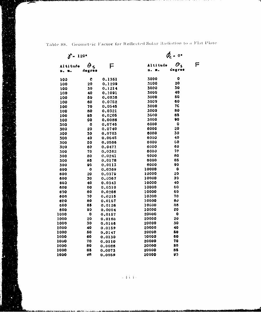
I'ale~C 88. (1colH tri .1 I i!L .) fo II tI clQ1, e d lar i oldtal to oa 1i1t lac

1200 0-"

Altitud* F Altitude &Sn.o. degree U. as degre*

100 0 0.1351 3000 0

100 20 0.1299 3000 20100 30 0.1214 3000 30

100 40 0.1091 3000 40100 50 0.0936 3000 50

100 60 0.0752 3009 60

100 70 0.0545 3000 7c

100 80 0.0321 3000 80100 88 0.0205 3000 85100 cO 0.0088 3000 90300 0 0.0748 0000 0300 20 0.0740 0000 20300 s0 0.0703 6000 30300 40 0.0645 6000 40300 50 0.0566 8000 bO300 G0 0.0471 6000 60

300 70 0.0362 6000 70300 80 0.0241 8000 80300 85 0.0178 6000 8s300 90 0.0113 8000 90

600 0 0.0369 10000 0600 20 0.0379 10000 20600 30 0.0367 10000 39603 40 0.0343 10000 40600 50 0.0310 10000 80

600 80 0.0268 10000 60000 70 0.0215 10300 70600 80 0.0157 10000 8.3600 85 0.0128 10000 85600 go 0.0094 10000 e0

1000 0 0.0157 20000 01000 20 0.0186 20000 20

1000 30 0.0168 20000 301000 40 0,015P 20000 401000 50 0.0147 20000 s0

1000 80 0.0130 20000 801000 70 0.0110 20000 701000 80 0.0086 20000 so1000 85 0.0073 20000 8s1000 Oft 0.005o 20000 00

cI

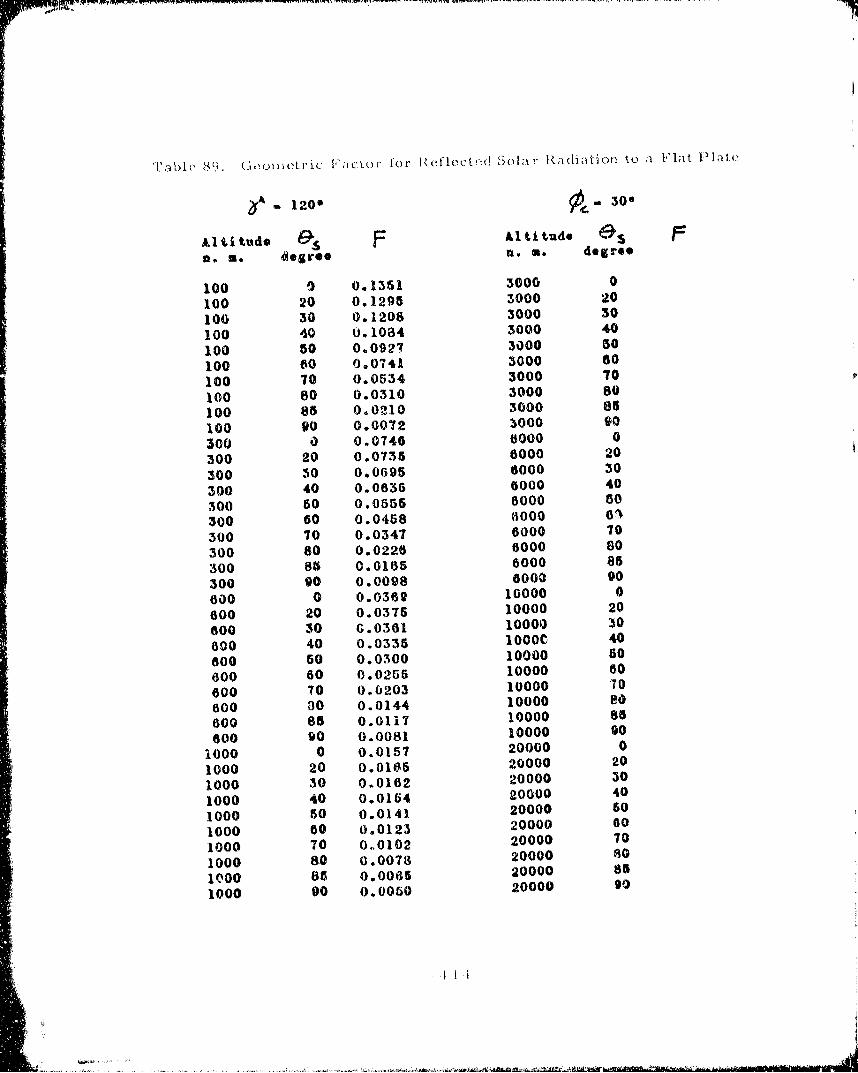
Tablei' 8) (wecjnletric IVactor for 1K.eflectý!d Sol.air Radiation to a Ilat Plat(.e

Al titude &s FAl ti tude as F

Ikem. egre 0. a. degree

100 0 0.1351 3000 0

100 20 0.129S 3000 20

100 30 0.1208 3000 30

100 40 0.1084 3000 40

100 50 0.0927 3000 30

100 60 0.0741 3000 60

100 70 0.0534 3000 70

100 80 0.0310 3000 80

100 88 0.0210 3000 85

100 g0 0.0072 3000 s0

300 0 0.0746 0000 0

300 20 0.07356 6000 20

300 s0 0.0695 6000 30

300 40 0.0635 0000 40

300 50 0.0555 6000 s0

300 60 0.0458 I000 01

300 70 0.0347 6000 70

300 80 0.0226 6000 80

300 85 0.0165 6000 85

300 90 0.0098 6000 90

600 0 0.0362 10000 0

600 20 0.0375 10000 20

600 30 G.0361 10000 30

800 40 0.0335 1000c 40

600 50 0.0100 10000 80

600 60 0.0255 10000 60

800 70 0.0203 10000 70

600 30 0.0144 10000 80

600 85 0.0117 10000 88

600 90 0.0081 10000 go

1000 0 0.0157 20000 0

1000 20 0.0165 20000 20

1000 30 0.0162 20000 30

1000 40 0.0154 20000 40

1000 50 0.0141 20000 60

1000 00 0.0123 20000 60

1000 70 0.0102 20000 70

1000 80 0.0078 20000 80

1000 88 0.0065 20000 85

1000 g0 0.0050 20000 90

:II I

- 20" 8

Altitude -as r Altitude Fno a. degree a. w. degree

100 0 0.1351 3000 0

100 20 0,1284 3000 20

100 30 0.1192 3000 30

100 40 0.1063 3000 40

100 50 0.0902 3000 80

100 60 0.0713 3000 60

100 70 0.0503 3000 70

100 80 0.0295 3000 80

100 85 0.0188 3000 so

100 90 0.0035 3000 90

300 0 0.0746 6000 0

300 20 0.0721 6000 20

300 30 0.0675 6000 30

300 40 0.0608 6000 40

300 60 0.0523 6000 50

300 00 0.0422 6000 60

300 70 0.0308 0000 70

300 80 0.0205 6000 80

o00 85 0.G148 6000 85

300 90 0.0537 6000 90

600 0 0.0309 10000 0

o00 20 0.0363 10000 20

600 30 0.0343 10000 30

600 40 0.0313 10000 40

600 50 0.0273 iO000 50

600 60 0.0225 10000 60600 70 0.0180 10000 70

600 80 0.0135 10000 80600 as 0.0105 10000 8B

600 90 o.o050 I400o 90

1000 0 0.0157 20000 0

1000 20 0.0158 20000 20

1000 30 0.0151 20000 30

1000 40 0.0140 20000 40

1000 50 0.0124 20000 501000 60 0.0104 20000 60

1000 70 0.0930 20000 70

1000 80 0.0820 20000 80

1000 8a 0.0700 20000 85

1000 80 0.0031 20000 90

'9' l 1;v 91. ( I I, I o 1 r . :to r ft 1. 14'!. L d Sol( o It WI L tII ,I ., Ioia t t t:

Altitude F &titudwn, m degrae. . m. degree

150 0 0. 3d1 3000 0100 20 0.269 1 2 00 20

100 30 0.1170 3000 30100 40 0.1034 3000 40

O0 50 0.0868 3000 50100 60 0.0675 3000 80100 70 0.0462 3000 7110G 80 0.0265 3000 80100 85 0.0160 3000 83100 90 0.0025 5000 90I00 0 0.0746 6000 0S00 20 0.0701 8000 20300 50 0.0646 1000 30300 40 0.0572 6000 40300 50 0.0419 8000 50300 80 0.0373 6000 60300 70 0.0280 6000 70300 80 0.0185 6000 80300 85 0.0128 6000 85zoo go 0.0040 6000 g0000 0 0.0369 10000 0o00 20 0.0347 10000 20600 30 0.0320 10000 30600 40 0.0283 10000 40600 s0 0.0237 1000)0 s0000 60 0.0184 10000 60600 70 0.0145 10000 70600 80 0.0112 10000 80600 85 0.0092 10000 85600 90 0,0035 10000 90

1000 0 0.0157 20000 01000 20 0.0148 20000 201000 30 0.0134 20000 301000 40 0.0120 20000 401000 50 0.0101 20000 s01000 60 0.0085 20000 601000 70 0.0073 20000 701000 80 0.0054 20000 801000 85 0.0040 20000 851000 90 0,0020 20000 s0

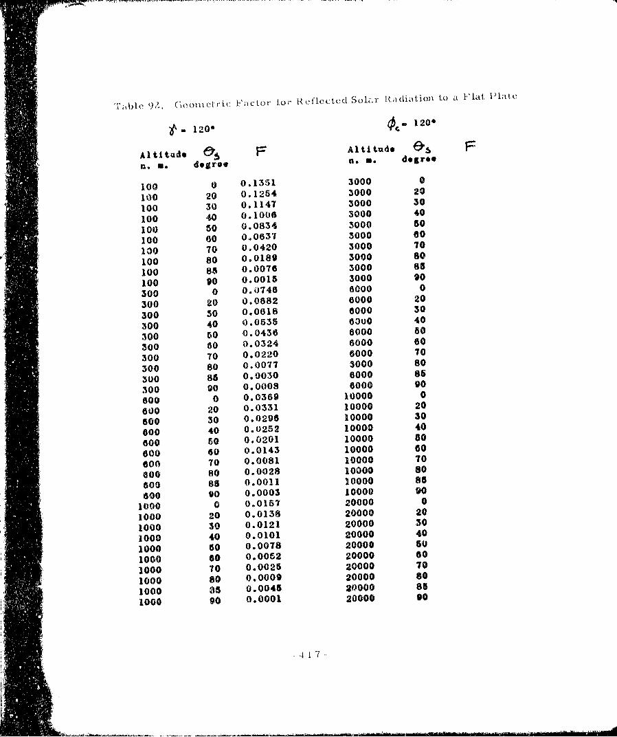
Tabhle )W, Geomletri. 'actor i:o- R efltcted Solar Radiatioll to a Fitat Platc

1 20 . 120

Altitude F Altitude gn. M. degree n. *. delree

100 0.1351 3000 0

100 20 0.1254 3000 20

100 30 0.1147 3000 30

100 40 0.1006 3000 40

100 50 0.0834 3000 50

100 60 0.0637 3000 80

130 70 0,0420 3000 70

100 80 0.0189 3000 80

100 88 0.0076 3000 85

100 90 0.0015 3000 90

300 0 0.0746 6000 0

300 20 0.0682 8000 20

300 3o 0.0618 o000 30

300 40 0.0535 0300 40

300 50 0.0436 8000 50

300 00 0.0324 6000 60

300 70 0.0220 6000 70

300 80 0.0077 3000 80

300 85 0.0030 0000 86

300 90 0.0008 6000 90

600 0 0.0369 10000 0

600 20 0.0331 10000 20

600 30 0.0296 10000 30

800 40 0.0252 10000 40

600 50 0.0201 10000 60

600 60 0.0143 10000 60

600 70 0.0081 10000 70

o00 80 0.0028 10000 80

600 65 0.0011 10000 85

o800 90 0.0003 10000 90

1000 0 0.0167 20000 0

1000 20 0.0138 20000 20

1000 3o 0.0121 20000 30

1000 40 0.0101 20000 40

1000 50 0.0078 20000 60

1000 60 0.0052 20000 60

1000 70 0.0025 20000 70

1000 80 0.0009 20000 s0

1000 35 0.0045 20000 85

1000 90 0.0001 20000 90

iI I *7

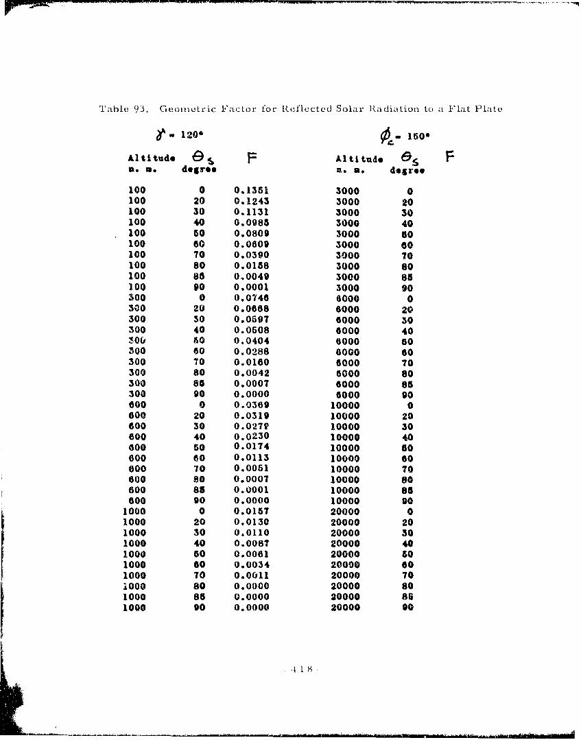
Table 93. Geometric Factor for Reflected Solar Radiation to a Flat Plate

e- 120" o- 150"

Altitude 194l F Al ti tude eu.e . degree a.s . degree

100 0 0.1351 3000 0100 20 0.1243 3000 20100 30 0.1131 3000 30100 40 0.0985 3000 40100 50 0.0809 3000 50100 60 0.0609 3000 60100 70 0.0390 3000 70100 80 0.0158 3000 80100 86 0,0049 3000 85100 90 0.0001 3000 90300 0 0.0746 6000 0300 20 0.0668 6000 20300 30 0.0597 6000 30300 40 0.0508 6000 40300 50 0.0404 0000 50300 60 0.0288 8000 60300 70 0.0160 6000 70300 80 0.0042 6000 80300 85 0.0007 6000 85300 90 0.0000 6000 90600 0 0.0369 10000 0800 20 0.0319 10000 20600 30 0.027V 10000 30600 40 0.0230 10000 40600 50 0.0174 10000 s0600 60 0.0113 10000 60000 70 0.0051 10000 70600 80 0.0007 10000 80600 85 0.0001 10000 88600 90 0.0000 10000 90

1000 0 0.0157 20000 01000 20 0.0130 20000 201000 30 0.0110 20000 30

1000 40 0.0087 20000 401000 50 0.0061 20000 s01000 80 0.0034 20000 601000 70 0.0011 20000 70iO00 80 0.0000 20000 801000 85 0.0000 20000 881000 90 0.0000 20000 904I1

Table 94. Geoni-et ric Factor for Reflecte~d Solar Raddiation to a I'lat Plate

-- 1200 1800

Altitude Os F Al ti tude GFn.o . degree n.o . degree

100 0 0.1351 3000 0100 20 0.1239 3000 20100 30 01125 3000 30100 40 0.0978 3000 40100 50 0.0800 3000 80100 60 0.0598 3000 s0100 70 0.0378 3000 TO100 80 0.0130 3000 80100 85 0.0024 3000 85100 go 0.0005 3000 g0300 0 0.0748 0000 0300 20 0.0662 6000 20300 30 0.0589 8000 30300 40 0.0499 6000 40300 50 0.0393 8000 50300 00 0.0275 6000 60300 70 0,0145 8000 70300 80 0.0024 6000 80300 85 0.0005 6000 85300 90 0.0001 6000 00600 0 0.0369 10000 0600 20 0.0314 10000 20t600 30 0.0272 10000 30600 40 0.0222 10000 40600 60 0.0184 10000 40600 60 0.0100 10000 60600 70 0.0040 10000 70600 80 0.0002 10000 80600 85 0.0000 10000 8B600 90 0.0000 10000 g01000 0 0.0157 20000 01000 20 0.0127 20000 201000 30 0.0108 20000 301000 40 0.0082 20000 401000 50 0.0055 20000 501000 80 0.0020 20000 601000 70 0.0000 20000 T01000 80 0.0000 20000 801000 85 0.0000 20000 851000 90 0.0000 20000 90

4 109

'f'able 9"). Gcometric f or 1\,-ticCtc!l Sola r [Vidi~itionl to a .1''lat PL-1te

Y.- 150,p0*-(

Altitude 9 F Al ti tide as F11. as degree Re *) degree

100 0 0.0144 3000 0100 20 0.0141 3000 20100 30 0.0132 3000 30100 40 0.0120 3000 40100 80 0.0104 3000 50100 80 0.0085 3000 60100 70 0.0084 3000 70100 80 0.0040 3000 80100 88 0.0028 3000 88100 g0 0.0018 3000 90300 0 0.0015 8000 0300 20 0.0018 8000 20300 50 0.0013 8000 30300 40 0.0014 8000 40300 50 0.0013 6000 50

300 80 0.0011 6000 80300 70 0.0009 6000 70300 80 0.0008 6000 8o300 85 0.0005 6000 85300 go 0.0004 6000 90600 0 10000 0800 20 10000 20800 30 10000 30800 40 10000 40800 50 1,0000 50800 60 10000 80600 70 10000 70800 80 10000 80800 85 10000 85800 90 10000 90

1000 0 20000 01000 20 20000 20

1000 30 20000 301000 40 20000 401000 50 20000 501000 80 20000 80

1000 70 20000 701000 80 20000 801000 85 20000 851000 g0 20000 g0

mA

Table 96�. Gcotu:et.ric Factor tot" Refhected, Solal;r Rdiatioi to a F'ý.at Plate

1" 1500 Oe 30"

Altitud P.4 r Al tJtud* 9- Fn. n. degroe a. e. s eree

100 0 0.0144 300 0100 20 O.Oi40 3000 20100 30 0.0131 3000 30100 40 0.0119 3000 40100 50 O.0103 3000 50100 60 0.0083 3000 60100 70 0.0062 3000 T0100 80 0.0038 3000 80100 88 0.0026 3000 8s100 90 0,0013 3000 90300 0 0.0016 6000 03C0 20 0.0016 6000 20300 30 0.0015 6000 30300 40 0.0014 0000 40300 50 0.0012 6000 80300 60 0.0011 6000 80300 70 0.0008 6000 70300 8o 0.0006 6000 80300 85 0.0008 6000 85300 90 0.0003 doco go600 0 10000 0000 20 10000 20600 30 10000 30800 40 10000 '40600 60 10000 60600 80 10060 60000 70 10000 70600 so 10000 80600 85 10000 BE600 90 10000 90

1000 0 20000 01000 20 20000 201000 30 20000 301000 40 20000 401000 so 20000 601000 60 20000 801000 70 20000 701000 80 20000 801000 86 20000 851000 90 20000 90

- 4 '

-. i a ii.e.i

Table 97. Geoneetric Factor for Reflected Solar Radiation to a Flat Plate

,V 10o" . 600

Altitude F Altitude, Fn.o . degree 1m2 . degree

100 0 0.0144 3000 0100 20 0.0138 3000 20

100 30 0.0129 3006 30

100 40 0.0115 3000 40

100 30 0.0098 3000 50

100 60 0.0079 3000 80

100 70 0.0036 3000 70

100 80 0.0032 3000 80100 83 0.0015 3000 88100 go 0.0008 3000 so

300 0 0.0015 6000 0300 20 0.0015 6000 20

300 s0 0.0014 6000 30

300 40 0.0013 6000 40

300 50 0.0011 6000 50

300 60 0.0009 0000 60300 70 0.0007 6000 70

300 80 0.0004 6000 80

300 86 0.0003 6000 88

o00 90 0.0002 6000 90

600 a 10000 0

800 20 10000 20

600 30 10000 30

A 40 10000 40

600 50 10000 60

000 80 10000 60600 70 10000 ?0

600 80 10000 so

600 85 10000 88

800 90 10000 go

1000 0 20000 0

1000 20 20000 20

1000 30 20000 30

1000 40 20000 40

1000 s0 20000 60

1000 60 20000 60

1000 70 20000 70

1000 80 20o00 8o

1000 s8 20000 as

-000 90 20000 90

. ,

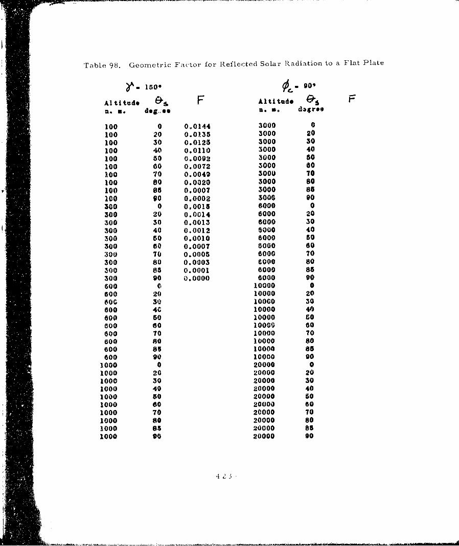
Table 98. Geometric Factor for Reflected Solar Radiation to a Flat Plate

)A . izOo Of g'

Altitude F Alti tud FSn.w. dog.. eu. so d.ree

100 0 0.0144 3000 0

100 20 0.0135 3000 20

100 30 0.0125 3000 30

100 40 0.0110 3000 40

100 50 0.0092 3000 50100 00 0.0072 3000 80

100 70 0.0049 3000 T0

100 80 0.0020 3000 80100 85 0.0007 3000 85100 90 0.0002 3000 90300 0 0.001's 0000 0

300 20 0.0014 6000 20300 30 0.0013 6000 30300 40 0.0012 6000 40300 50 0.0010 6000 50300 60 0.0007 6000 60

30U 70 0.0005 6000 70300 80 0.0003 @000 80300 88 0.0001 8000 85300 90 0.0000 6000 90

600 0 10000 0o00 20 10000 20800 30 10000 30600 4G 10000 40800 50 10000 s0600 60 10000 80o00 70 10000 70600 80 10000 80600 85 10000 86600 10 10000 90

1]000 0 20000 01000 20 20000 201000 30 20000 301000 40 20000 401000 50 20000 601000 60 20000 601000 70 20000 701000 80 20000 801000 85 20000 851000 to 20000 90

4 2 3

Table 99. Geometric Factor for Reflected Solar Radiation to a Flat Plate

e-. 150" O€-120"

Altitude 194 F Altitude es F.3 m. degree n. m. degree

100 0 0.0144 3000 0100 20 0.0133 3000 20100 30 0.0121 3000 30100 40 0.0105 3600 40100 50 0.0086 3000 50100 60 0.0065 3000 00100 70 0.0042 3000 70100 80 0.0017 3000 80100 88 0.0004 3000 85100 90 0.0000 3000 90300 0 0.0015 6000 0300 20 0.0014 8000 20300 30 0.0012 0000 30300 40 0.0010 0000 40300 50 0.0008 6000 50300 60 0.0006 6000 60300 70 0.0004 6000 70300 80 0.0000 8000 80300 85 0.0000 6000 85300 00 0.0000 0000 90600 0 10000 0800 20 10000 20600 30 10000 30800 40 10000 40800 so 10000 80800 60 10000 60600 70 10000 70800 80 10000 80600 85 10000 85600 90 10000 90

1000 0 20000 01000 20 20000 201000 30 20000 301000 40 20000 401000 50 20000 501000 60 20000 601000 70 20000 701000 80 20000 so1000 85 20000 851000 90 20000 90

I$ Iill raI

Si ' i

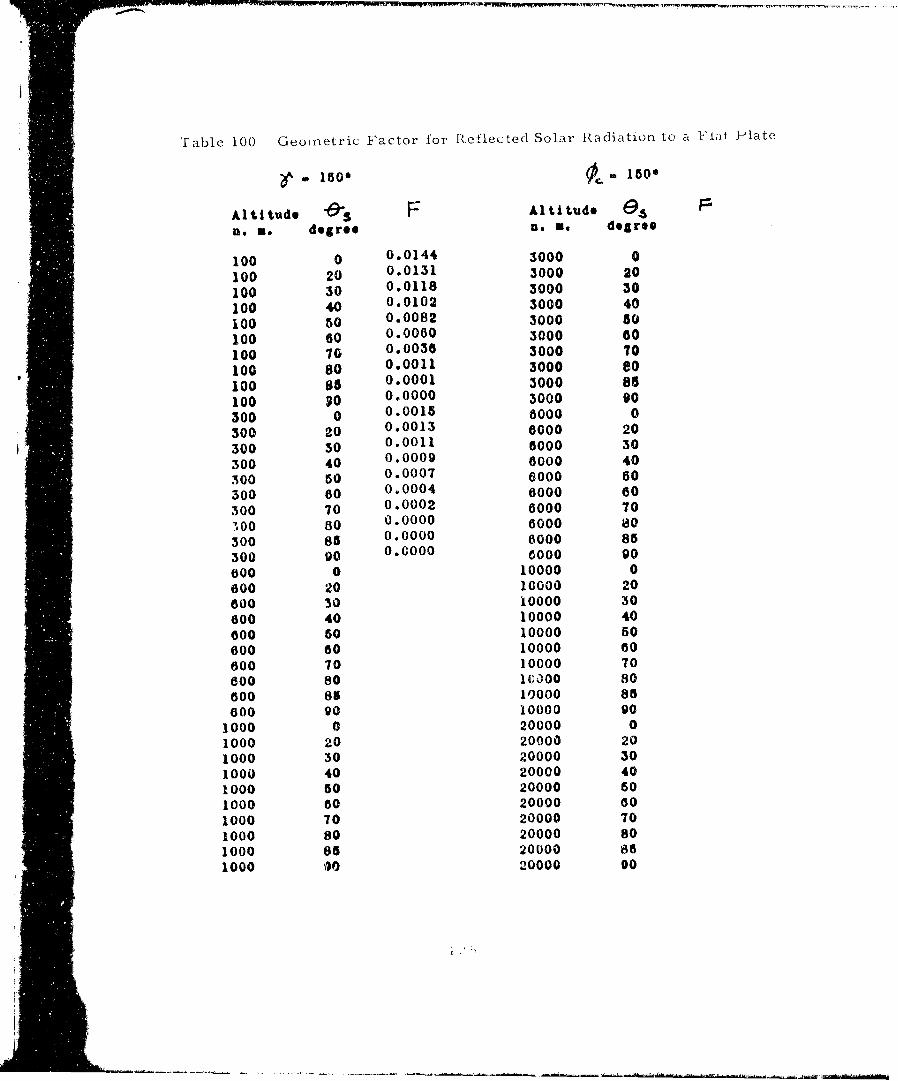
Table 100 Geometric Factor for Reflected Solar Radiation to a ijAi Plate

*1500 1500

Altitude -Al F Altitude 86n.*. degree n. m. degree

100 0 0.0144 3000 0100 20 0.0131 3000 20

100 30 0.0118 3000 30100 40 0.0102 3000 40

iO0 50 0.0082 3000 50

100 60 0.0060 3000 80

100 70 0.0036 3000 70

100 80 0.0011 3000 80100 88 0.0001 3000 85100 80 0.0000 3000 a0

300 0 0.0010 8000 0300 20 0.0013 8000 20300 20 0.0011 8000 30300 40 0.0009 8000 40300 50 0.0007 6000 80300 80 0.0004 6000 80300 70 0.0002 6000 70300 80 0.0000 6000 80300 85 0.0000 6000 85300 80 0.0000 0000 906000 0 10000 0800 20 10000 20800 30 10000 30800 40 10000 40800 50 10000 60600 50 10000 80800 70 10000 70600 80 10000 80600 85 1000 88800 90 10000 90

1000 g 20000 01000 20 20000 201000 30 20000 301000 40 20000 401000 50 20000 501000 50 20000 501000 70 20000 701000 80 20000 801000 85 20000 85

1000 90 20000 90

i i ii•-

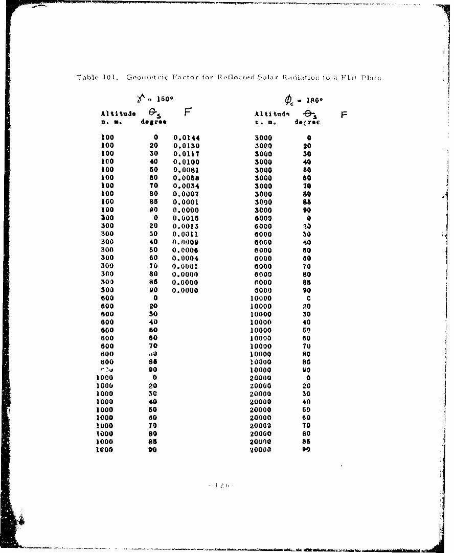
Table 101. Geomnetric FVactor for Reflected Solar Rudiiation to a F'lat P lite IAlits Al i 0d -&iso

DO degree M. m. del rec

100 0 0.0144 3000 0100 20 0.0130 30O0 20100 30 0.0117 3000 30ICO 40 0.0100 3000 40100 50 0.0081 3000 s0100 60 0.0068 3000 80100 70 0.0034 3000 70100 80 0.0007 3000 80100 85 0.0001 3000 85100 90 0.0000 3000 90300 0 0.0015 8000 0300 20 0.0013 6000 10300 30 0.0011 6000 30 I300 40 010009 80C0 40300 50 0.0006 8000 50300 60 0.0004 6000 00300 70 0.0001 0000 T0

300 80 0.0000 6000 80300 85 0.0000 000 85300 90 0.0000 0000 90600 0 10000 C600 20 10000 20600 30 10000 30600 40 10000 40600 60 10000 60800 60 10000 60600 70 10000 70600 jO 10000 80600 85 10000 85'x. go 10000 90

1000 0 20000 0100 20 20000 201000 30 20000 301000 40 20000 401000 50 20000 601000 80 20000 80luO0 70 20000 701000 80 20000 801000 88 20000 851000 90 20000 90

i t 2.,-