radiation impedance of capacitive micromachined ultrasonic transducers
TRANSCRIPT

RADIATION IMPEDANCE OF CAPACITIVEMICROMACHINED ULTRASONIC
TRANSDUCERS
a dissertation submitted to
the department of electrical and electronics
engineering
and the institute of engineering and science
of bilkent university
in partial fulfillment of the requirements
for the degree of
doctor of philosophy
By
Muhammed N. Senlik
January 29, 2010

I certify that I have read this thesis and that in my opinion it is fully adequate,
in scope and in quality, as a dissertation for the degree of doctor of philosophy.
Prof. Dr. Abdullah Atalar (Supervisor)
I certify that I have read this thesis and that in my opinion it is fully adequate,
in scope and in quality, as a dissertation for the degree of doctor of philosophy.
Prof. Dr. Hayrettin Koymen
I certify that I have read this thesis and that in my opinion it is fully adequate,
in scope and in quality, as a dissertation for the degree of doctor of philosophy.
Prof. Dr. Orhan Aytur
ii
I certify that I have read this thesis and that in my opinion it is fully adequate,
in scope and in quality, as a dissertation for the degree of doctor of philosophy.
Prof. Dr. Cemal Yalabık
I certify that I have read this thesis and that in my opinion it is fully adequate,
in scope and in quality, as a dissertation for the degree of doctor of philosophy.
Assist. Prof. Dr. Ayhan Bozkurt
Approved for the Institute of Engineering and Science:
Prof. Dr. Mehmet BarayDirector of Institute of Engineering and Science
iii

in loving memory of my mother
iv

ABSTRACT
RADIATION IMPEDANCE OF CAPACITIVEMICROMACHINED ULTRASONIC TRANSDUCERS
Muhammed N. Senlik
Ph.D. in Electrical and Electronics Engineering
Supervisor: Prof. Dr. Abdullah Atalar
January 29, 2010
Capacitive micromachined ultrasonic transducers (cMUTs) are used to transmit
and receive ultrasonic signals. The device is constructed from circular membranes
fabricated with surface micromachining technology. They have wider bandwidth
with lower transmit power and lower receive sensitivity compared to the piezo-
electric transducers, which dominate the ultrasonic transducer market. In order
to be commercialized, they must overcome these drawbacks or find new applica-
tion areas, where piezoelectric transducers perform poorly or cannot work. In this
thesis, the latter approach, finding a new application area, is followed to design
wide band and highly efficient airborne transducers with high output power by
maximizing the radiation resistance of the transducer.
The radiation impedance describes the interaction of the transducer with the
surrounding medium. The real part, radiation resistance, is a measure of the
amount of the power radiated to the medium; whereas the imaginary part, ra-
diation reactance, shows the wobbled medium near the transducer surface. The
radiation impedance of cMUTs are currently not well-known. As a first step,
the radiation impedance of a cMUT with a circular membrane is calculated ana-
lytically using its velocity profile up to its parallel resonance frequency for both
the immersion and the airborne applications. The results are verified by finite
element simulations. The work is extended to calculate the radiation impedance
of an array of cMUT cells positioned in a hexagonal pattern. The radiation
impedance is determined to be a strong function of the cell spacing. It is shown
that excitation of nonsymmetric modes is possible in immersion applications.
A higher radiation resistance improves the bandwidth as well as the efficiency
and the transmit power of the cMUT. It is shown that a center-to-center cell spac-
ing of 1.25 wavelength maximizes the radiation resistance for the most compact
arrangement, if the membranes are not too thin. For the airborne applications,
the bandwidth can be further increased by using smaller device dimensions, which
v
vi
decreases the impedance mismatch between the cMUT and the air. On the other
hand, this choice leads to degradation in both efficiency and transmit power due
to lowered radiation resistance. It is shown that by properly choosing the ar-
rangement of the thin membranes within an array, it is possible to optimize the
radiation resistance. To make a fair analysis, same size arrays are compared. The
operating frequency and the collapse voltage of the devices are kept constant. The
improvement in the bandwidth and the transmit power can be as high as three
and one and a half times, respectively. This method may also improve the noise
figure when cMUTs are used as receivers. A further improvement in the noise
figure is possible when the cells are clustered and connected to separate receivers.
The results are presented as normalized graphs to be used for arbitrary device
dimensions and material properties.
Keywords: Capacitive Micromachined Ultrasonic Transducer (cMUT), Analyti-
cal Modeling, Finite Element Method (FEM) Modeling, Radiation Impedance,
Airborne cMUT.

OZET
KAPASITIF MIKROISLENMIS ULTRASONIKCEVIRICILERIN RADYASYON EMPEDANSI
Muhammed N. Senlik
Elektrik ve Elektronik Muhendisligi, Doktora
Tez Yoneticisi: Prof. Dr. Abdullah Atalar
29 Ocak 2010
Kapasitif mikroislenmis ultrasonik ceviriciler (cMUT) ultrasonik sinyallerin
yayımında ve alımında kullanılmaktadırlar. Cihaz, yuzey mikroisleme teknolo-
jisi ile uretilmis dairesel zarlardan imal edilmistir. Ultrasonik cevirici pazarını
domine eden piezoelektrik ceviriciler ile karsılastırıldıklarında daha genis bant
genisligine sahip olmakla birlikte daha dusuk yayım gucu ile daha dusuk alım
hassasiyetine sahiptirler. Ticarilestirilebilmeleri icin bu eksikliklerinin giderilmesi
ya da piezoelektrik ceviricilerin kotu calıstıgı veya calısamadıgı alanlarda uygu-
lamalar bulmaları gerekmektedir. Bu tezde, bu yollardan ikincisi, ceviricinin
radyasyon rezistansını en yuksek hale getirerek genis bantlı, yuksek verimli
ve yuksek yayım gucune sahip havada calısan cMUT’ların tasarımı amacıyla
izlenmistir.
Radyasyon empedansı ceviricinin cevresindeki ortam ile olan etkilesimini
tanımlamaktadır. Gercek kısmı, radyasyon rezistansı, ortama yayımlanan gucun
bir olcusu iken sanal kısmı, radyasyon reaktansı, cevirici yuzeyinde calkalanan
ortamı gostermektedir. Su anda cMUT’ların radyasyon empedansı iyi bir sekilde
bilinmemektedir. Ilk adım olarak, dairesel zara sahip cMUT’ların hız profilleri
kullanılarak paralel rezonans frekansına kadarki radyasyon empedansları su ve
hava uygulamaları icin hesaplanmıstır. Sonuclar sonlu eleman simulasyonları ile
dogrulanmıstır. Calısma altıgen bir yapı olusturacak sekilde hucrelerden mey-
dana gelen bir dizinin radyasyon empedansını hesaplamak icin genisletilmistir.
Radyasyon empedansının hucreler arasındaki mesafenin kuvvetli bir fonksi-
yonu oldugu bulunmustur. Su uygulamalarında simetrik olmayan modların
uyarılmasının mumkun oldugu gosterilmistir.
Daha yuksek bir radyasyon rezistansı bant genisligiyle birlikte verimi ve
yayım gucunu arttırmaktadır. En yogun yerlesim duzeninde, hucreler arasındaki
mesafe dalgaboyunun 1.25 katı oldugu zaman radyasyon rezistansı ince zarlar
vii

viii
icin en yuksek degerine ulasmaktadır. Hava uygulamaları icin, cihaz boyut-
ları kucultulerek cMUT ve hava arasındaki empedans uyumsuzlugu azaltılıp
bant genisligi arttırılabilmektedir. Obur yandan, bu secim radyasyon rezis-
tansının degerini azaltması nedeniyle verimi ve yayım gucunu dusurmektedir.
Ince zara sahip cMUT’ların dizi icerisindeki yerlesimi duzenlenerek radyasyon
rezistansının en iyilestirilebilecegi gosterilmistir. Adil bir analiz yapabilmek
icin, aynı alana sahip diziler karsılastırılmıstır. Cihazların calısma frekansları
ve cokme voltajları sabit tutulmustur. Bant genisligi ve yayım gucundeki i-
yilesme uc ve bir bucuk kat daha yuksek olabilmektedir. Bu metod cMUT’lar
almac olarak kullanıldıklarında da gurultu performanslarını iyilestirmektedir.
Gurultu performansı, hucreler kumelendirilip farklı almaclara baglandıgında daha
da arttırılabilmektedir. Sonuclar herhangi bir cihaz boyutu ve malzeme ozelligi
icin kullanılabilmeleri amacıyla normalize grafikler halinde sunulmustur.
Anahtar sozcukler : Kapasitif Mikroislenmis Ultrasonik Cevirici (cMUT), Analitik
Modelleme, Sonlu Eleman Metodu (SEM) ile Modelleme, Radyasyon Empedansı,
Havada Calısan cMUT.
ACKNOWLEDGEMENTS
I would like to express my sincere gratitude to Prof. Atalar for his supervision,
guidance and encouragement through the development of this thesis. He was the
perfect supervisor for me.
I would like to thank to the members of my thesis jury for reading the
manuscript and commenting on the thesis.
Selim and Elif, there are no words to describe them or no ways to thank them.
Endless thanks to Emre Kopanoglu and Onur Bakır for their supports. I must
also thank to my labmates, Burak, Ceyhun, Deniz, Kagan and Vahdet, who have
to see my Gargamel face everyday.
Many thanks to my friends, students and professors, whose names I forgot to
mention. Some times, a little smile makes my day.
Without my family, this work would be never be possible.
Finally, my brother, Servet. Although I am the elder one, he was both a father
and a mother for me. Thanks for always being there.
ix

Contents
1 INTRODUCTION 1
1.1 Analysis . . . . . . . . . . . . . . . . . . . . . . . . . . . . . . . . 2
1.1.1 Modeling . . . . . . . . . . . . . . . . . . . . . . . . . . . 2
1.1.2 Radiation Impedance . . . . . . . . . . . . . . . . . . . . . 3
1.2 Applications . . . . . . . . . . . . . . . . . . . . . . . . . . . . . . 4
2 FUNDAMENTALS of cMUT 6
2.1 cMUTs . . . . . . . . . . . . . . . . . . . . . . . . . . . . . . . . . 6
2.2 Modeling . . . . . . . . . . . . . . . . . . . . . . . . . . . . . . . . 7
2.2.1 Analytical Modeling . . . . . . . . . . . . . . . . . . . . . 8
2.2.2 Finite Element Method (FEM) Modeling . . . . . . . . . . 13
3 RADIATION IMPEDANCE 15
3.1 Mechanical Behavior of a Circular cMUT Membrane . . . . . . . 15
3.1.1 Velocity Profile . . . . . . . . . . . . . . . . . . . . . . . . 15
3.1.2 Radiation Impedance . . . . . . . . . . . . . . . . . . . . . 16
x
CONTENTS xi
3.2 Radiation Impedance of an Array of cMUT Cells . . . . . . . . . 21
3.2.1 Mutual Radiation Impedance between Two cMUT Cells . 21
3.2.2 Radiation Impedance of an Array of cMUT Cells . . . . . 22
4 AIRBORNE cMUTs 27
4.1 Performance Figures . . . . . . . . . . . . . . . . . . . . . . . . . 27
4.1.1 Radiation Resistance . . . . . . . . . . . . . . . . . . . . . 28
4.1.2 Q Factor . . . . . . . . . . . . . . . . . . . . . . . . . . . . 29
4.1.3 Transmit Mode . . . . . . . . . . . . . . . . . . . . . . . . 30
4.1.4 Receive Mode . . . . . . . . . . . . . . . . . . . . . . . . . 31
4.1.5 Noise Analysis . . . . . . . . . . . . . . . . . . . . . . . . . 33
4.2 Design Examples . . . . . . . . . . . . . . . . . . . . . . . . . . . 35
5 CONCLUSION 37

List of Figures
1.1 3D view of a cMUT cell. . . . . . . . . . . . . . . . . . . . . . . . 1
2.1 (a) Cross-section of a single cMUT cell fabricated with a low tem-
perature fabrication process. (b) Close view of a fabricated array.
The light and the dark gray regions show the membrane and the
electrode. Fig. 2.1(a) is the cross section of this region. . . . . . . 7
2.2 (a) Deflection of the center of the membrane with respect to the
applied voltage. Arrows indicate the direction of the movement as
the voltage is changed. (b) Membrane shapes for various voltages
just around collapse and snap-back. Region 1 and 2 are before
and during collapse, respectively. The radius and the thickness of
the membrane and the gap height are 20 µm, 1 µm and 0.2 µm,
respectively. The membrane material is Si3N4. . . . . . . . . . . . 8
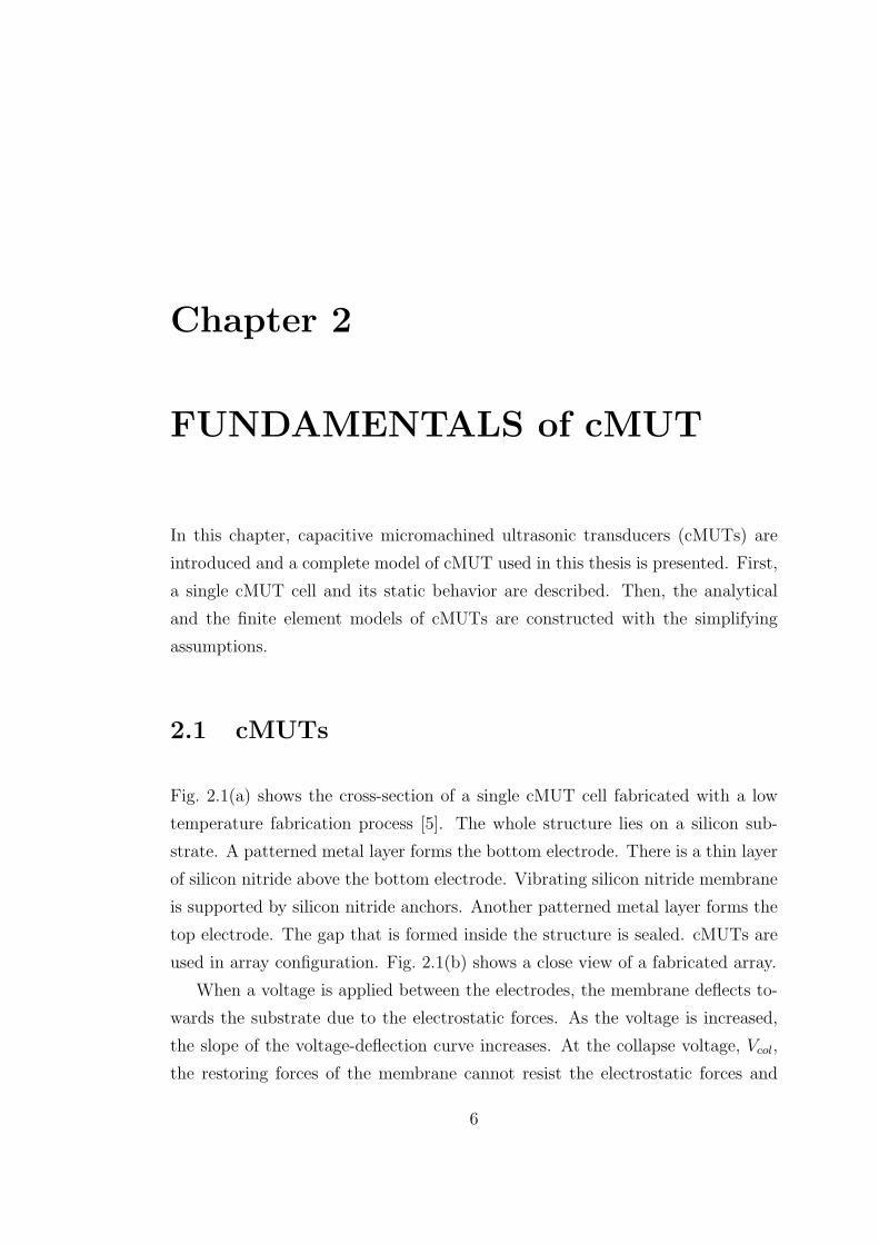
2.3 cMUT used in (a) transmit and (b) receive configurations. In both
configurations, cMUT is DC biased with a source and a resistor.
During the transmission, a pulse is applied over a capacitor and
during the reception an amplifier is connected through a capacitor. 9
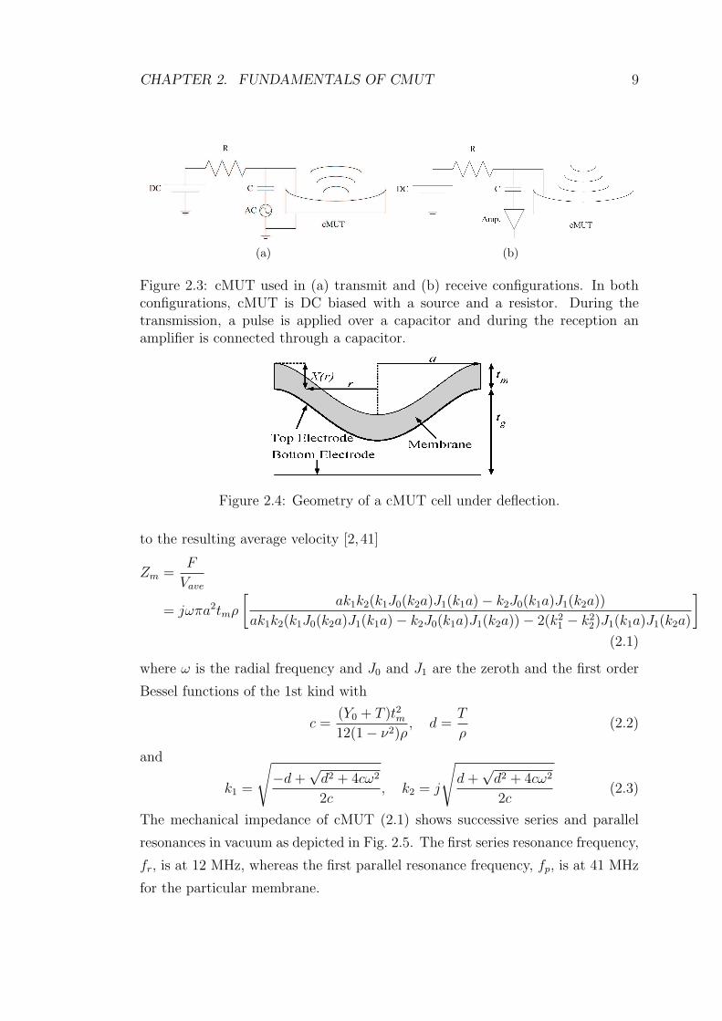
2.4 Geometry of a cMUT cell under deflection. . . . . . . . . . . . . . 9
2.5 Mechanical impedance of cMUT in vacuum. a=20 µm and
tm=1 µm. The membrane material is Si3N4 and T=0 Pa. . . . . . 10
xii
LIST OF FIGURES xiii
2.6 Mason’s equivalent circuit of cMUT. C is the shunt input capac-
itance and n is the turns ratio. The membrane impedance up to
0.4fp is modelled with a series LC section. During the reception,
cMUT is excited by a force source with an amplitude of PS, where
P is the incident pressure field. . . . . . . . . . . . . . . . . . . . 12
2.7 Directivity of (a) a single cell (b) array in Fig. 3.3. ka=2 for the
cMUT cell. . . . . . . . . . . . . . . . . . . . . . . . . . . . . . . 13
3.1 (a) The velocity profiles of rigid piston, simply supported and
clamped radiators normalized to the peak values (b) The veloc-
ity profiles of a cMUT membrane normalized to the peak values
determined by FEM simulations at f=0.2fp, 0.4fp and fp. The
same profiles approximated using (3.3) with [α2=0.94, α4=0.06],
[α2=0.71, α4=0.3] and [α2=-2.45, α4=3.06] are also shown. . . . . 17
3.2 The calculated radiation (a) resistance (b) reactance normalized by
Sρ0c0 of a piston radiator, a clamped radiator and cMUT mem-
branes with kpa=π, 2π and 4π. The radiation impedances of the
cMUT membranes determined by FEM simulations (circles) are
also included. The curves for cMUT membranes are shown for
ka ≤ kpa. . . . . . . . . . . . . . . . . . . . . . . . . . . . . . . . 19
3.3 The geometry of a circular array with hexagonally placed N=7
cells and d=2a. . . . . . . . . . . . . . . . . . . . . . . . . . . . . 22
3.4 The equivalent circuit of the radiation impedance for (a) a general
array and (b) a circular array with hexagonally placed N=7 cells. 23
3.5 The representative radiation resistance, Rr, normalized by Sρ0c0
of a single cMUT cell in N=7, 19, 37 and 61 element arrays in
comparison to a cell in N=19 element piston array all with a/d=0.5
as a function of kd for a cMUT cell with (a) kpa=2π and (b)
kpa=4π. The representative radiation resistance determined by
FEM simulations (circles) are also shown. . . . . . . . . . . . . . 24

LIST OF FIGURES xiv
3.6 kdopt and normalized Rmax as a function of a/d for a cMUT cell
with kpa=4π in N=7, 19, 37 and 61 element arrays. . . . . . . . . 25
3.7 (a) The representative radiation resistance normalized by Sρ0c0 of
a single cMUT cell in N=7 element array in water for a cell with
d=2.1a, kpa=2.15 and 3.7. The representative radiation resistance
determined by FEM simulations (circles) are also depicted. Note
that the kpa=2.15 curve does not have the kdopt=7.5 peak. The
discrepancy between FEM simulations and analytic curve is due to
the presence of antisymmetric mode. (b) FEM computed velocity
profile of the cells showing the excitation of antisymmetric mode
at the outer cells for kpa=2.15 and kd=2.4. . . . . . . . . . . . . . 26
4.1 The geometry of a circular array with hexagonally placed N=19
cells. . . . . . . . . . . . . . . . . . . . . . . . . . . . . . . . . . . 28
4.2 (a) The normalized radiation resistance (Rn) of a single cell in
various arrays as a function of d/a. (b) The change of the optimum
separation (dopt) and the maximum normalized radiation resistance
(Rmax) as a function of a/λr. . . . . . . . . . . . . . . . . . . . . . 29
4.3 Q of various arrays as a function of d/a. . . . . . . . . . . . . . . 30
4.4 The average output power normalized by λr and Vcol per unit area
of various arrays as a function of d/a. . . . . . . . . . . . . . . . . 31
4.5 (a) Rin (b) Cin normalized by λr and Vcol per unit area of various
arrays as a function of d/a. . . . . . . . . . . . . . . . . . . . . . . 33
4.6 The receiver circuitry used in the calculations of the noise figure,
OPAMP with (a) non-inverting (b) inverting configurations. . . . 34
4.7 F of various receiver circuitries as a function of Rs. (a) BJT (b)
FET OPAMP . . . . . . . . . . . . . . . . . . . . . . . . . . . . . 35

List of Tables
2.1 Material parameters used in the simulations. . . . . . . . . . . . . 10
3.1 Variation of α2 and α4 with respect to f/fp. . . . . . . . . . . . . 17
3.2 Constants and functions used in (3.8). . . . . . . . . . . . . . . . 20
3.3 Small argument approximations of the real and the imaginary parts
of Pnm/Sρ0c0V2rms in (3.8). (y=ka) . . . . . . . . . . . . . . . . . 21
4.1 Reduction in noise figure (dB). . . . . . . . . . . . . . . . . . . . 35
4.2 The comparison of the most compact and the sparse arrangements. 36
xv
Chapter 1
INTRODUCTION
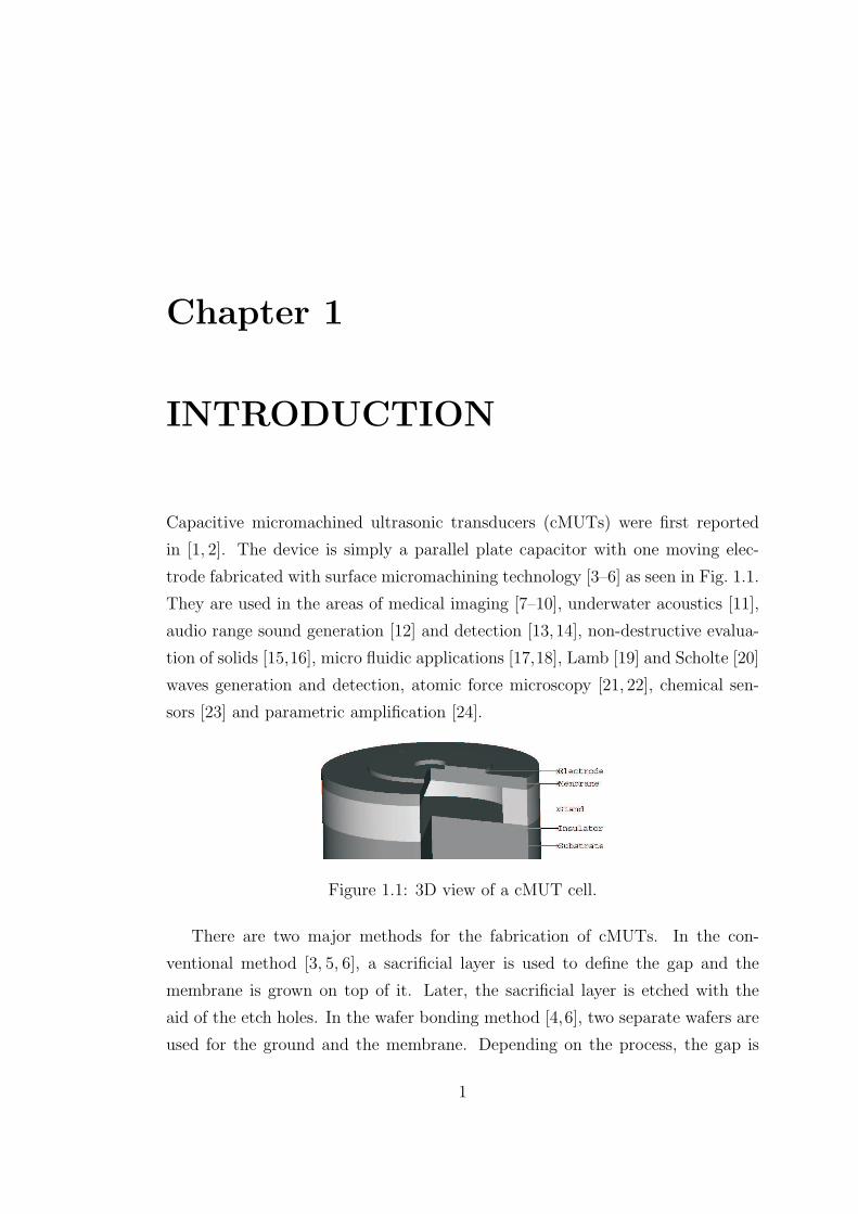
Capacitive micromachined ultrasonic transducers (cMUTs) were first reported
in [1, 2]. The device is simply a parallel plate capacitor with one moving elec-
trode fabricated with surface micromachining technology [3–6] as seen in Fig. 1.1.
They are used in the areas of medical imaging [7–10], underwater acoustics [11],
audio range sound generation [12] and detection [13,14], non-destructive evalua-
tion of solids [15,16], micro fluidic applications [17,18], Lamb [19] and Scholte [20]
waves generation and detection, atomic force microscopy [21, 22], chemical sen-
sors [23] and parametric amplification [24].
Figure 1.1: 3D view of a cMUT cell.
There are two major methods for the fabrication of cMUTs. In the con-
ventional method [3, 5, 6], a sacrificial layer is used to define the gap and the
membrane is grown on top of it. Later, the sacrificial layer is etched with the
aid of the etch holes. In the wafer bonding method [4,6], two separate wafers are
used for the ground and the membrane. Depending on the process, the gap is
1

CHAPTER 1. INTRODUCTION 2
defined on one of the wafers. Then, these wafers are bonded with a wafer bonder.
It is possible to fabricate cMUTs using a foundry [25–27], however this process
lacks the sealing of the membranes. Also, each research group developed their
fabrication processes based on these methods.
Compatibility with silicon IC technology and ease of construction of ar-
rays made cMUTs an alternative to piezoelectric tranducers, which are cur-
rently used in most of the applications mentioned above. cMUTs offer wider
bandwidth [28, 29], however, they provide approximately 10-dB lower loop
gain [28, 29] 1 compared to their alternatives which is one of the reasons not
to be commercialized. There are various techniques to increase the loop gain of
cMUTs. These are changing the membrane structure [30–35], operating in dif-
ferent regimes [36], use of different detection techniques [23, 37, 38] and use of
different electrical circuitry [39,40]. However, each method brings disadvantages,
such as high operating voltages or an extra detection structure, which may not
be silicon compatible.
1.1 Analysis
1.1.1 Modeling
The modeling is an important tool to characterize and design transducers. There
are two approaches followed in the modeling of cMUTs, analytical modeling
and modeling with finite element method (FEM) simulations. The former one
starts with the solution of the differential equation governing the membrane mo-
tion [2, 41]. Then, an equivalent circuit known as Mason’s equivalent circuit is
constructed. The parameters of these equivalent circuit is obtained from the
above solution together with the actual device dimensions. In [42,43], the trans-
formers ratio of cMUT is calculated and in [1,2,44,45], the mechanical impedance
1The loop gain is defined as the ratio of the received voltage to the applied voltage inpulse-echo mode.

CHAPTER 1. INTRODUCTION 3
of the membrane is replaced with a series LC section. Yaralioglu et al. [46], Ron-
nekleiv [47] and Senlik et al. [48] calculated the radiation impedance of the mem-
brane. In the latter approach, the complete model of cMUT is implemented with
a commercially available software package [49–51] or a cMUT specific tool [52].
Also it is possible to implement the equations governing cMUT operation with a
circuit analysis tool [53,54] to construct an equivalent circuit.
In this thesis, the analytical approach followed in [48, 55] is used with the
simplifying assumptions. The FEM simulations are used only for the verification
purposes.
1.1.2 Radiation Impedance
The radiation impedance describes the interaction of the transducer with the
surrounding medium. The real part, the radiation resistance, denotes the quanti-
tative amount of the power radiated to the medium; whereas the imaginary part,
the radiation reactance, shows the quantitative stored energy in the near field.
The radiation impedance of cMUTs are currently not well-known. In this thesis,
the radiation impedance of cMUTs with circular membranes is calculated.
The mechanical impedance of a cMUT membrane in vacuum is well stud-
ied [45]. It shows successive series and parallel resonances, where force and ve-
locity becomes zero, respectively [56]. When a cMUT is immersed in water, the
acoustic loading on the cell is high and results in a wide bandwidth. All mechan-
ical resonance frequencies shift to lower values because of the imaginary part of
the radiation impedance. If a cMUT is used in air, the radiation impedance is
rather low and the bandwidth is limited by the mechanical Q of the membrane. It
is therefore preferable to increase the radiation resistance in order to get a higher
bandwidth in airborne applications. Moreover, for the same membrane motion,
a higher acoustic power is delivered to the medium, if the radiation resistance is
higher. Hence, a higher radiation resistance is desirable to be able to transmit
more power, since the gap limits the maximum allowable membrane motion.
The efficiency of a transducer is defined as the ratio of the power radiated to
the medium to the power input to the transducer [57]. The loss in a cMUT due
CHAPTER 1. INTRODUCTION 4
to the electrical resistive effects and the mechanical power lost to the substrate
can be represented as a series resistance [1]. Hence, the efficiency will increase if
the radiation resistance increases in both airborne and immersion cMUTs, since
a smaller portion of the energy will be dissipated on the loss mechanisms such as
the coupling into the substrate.
There are several approaches to model the radiation impedance of the cMUT
membrane. In [46], the radiation impedance is modelled using an equal size piston
radiator. In [58], an equivalent piston radiator with the appropriate boundary
conditions is defined and its radiation impedance is used. In [59, 60], the radi-
ation impedance of an array is modelled with lumped circuit elements. In [61],
the radiation impedance is calculated by subtracting the mechanical impedance
of the membrane from the input mechanical impedance as computed by a finite
element simulation. In [47], cMUT is modelled with a modal expansion based
method and the radiation impedance is calculated using that method. Caronti et
al. [62] calculated the radiation impedance of an array of cells performing finite
element method simulations with a focus on the acoustic coupling between the
cells.
1.2 Applications
Airborne ultrasound has many applications in diverse areas, generally requiring
high bandwidth. The impedance mismatch between air and the transducer causes
a reduction of bandwidth of the device. cMUTs offer wider bandwidth in air com-
pared to the piezoelectric counterparts at the expense of lower transmit power
and receive sensitivity. In this thesis, the bandwidth of cMUT operating in air is
optimized without degrading the transmit and the receive performance.
cMUTs used in air require membranes with high radius-to-thickness ratios
and high gap heights due to the frequency requirements and the effect of the at-
mospheric pressure. The conventional fabrication of cMUTs, the sacrificial layer
method [3,5] does not allow the fabrication of these large membranes [4, 6]. The
use of the wafer bonding technology [4] and the optimization of the process make
possible the production of the reliable cMUTs operating in air.
CHAPTER 1. INTRODUCTION 5
There are various methods to increase the bandwidth of cMUTs. Using thin-
ner membranes decreases the membrane impedance and hence reduces the quality
factor [63]. Introducing lossy elements to the electrical terminals of the device
may also work at the expense of reduced efficiency and sensitivity. On the other
hand, increasing the radiation resistance also helps without causing a reduction
in the efficiency [48,64] as mentioned previously.
Chapter 2 gives the fundamentals and the basic operation principles of cMUT.
This chapter also includes the modelling used throughout this thesis. Chapter 3
presents the calculation of the radiation impedance of cMUT by analytical means.
Chapter 4 describes the application of the model to design wide band, highly ef-
ficient airborne cMUTs with high output power. The last chapter concludes this
thesis.
Chapter 2
FUNDAMENTALS of cMUT
In this chapter, capacitive micromachined ultrasonic transducers (cMUTs) are
introduced and a complete model of cMUT used in this thesis is presented. First,
a single cMUT cell and its static behavior are described. Then, the analytical
and the finite element models of cMUTs are constructed with the simplifying
assumptions.
2.1 cMUTs
Fig. 2.1(a) shows the cross-section of a single cMUT cell fabricated with a low
temperature fabrication process [5]. The whole structure lies on a silicon sub-
strate. A patterned metal layer forms the bottom electrode. There is a thin layer
of silicon nitride above the bottom electrode. Vibrating silicon nitride membrane
is supported by silicon nitride anchors. Another patterned metal layer forms the
top electrode. The gap that is formed inside the structure is sealed. cMUTs are
used in array configuration. Fig. 2.1(b) shows a close view of a fabricated array.
When a voltage is applied between the electrodes, the membrane deflects to-
wards the substrate due to the electrostatic forces. As the voltage is increased,
the slope of the voltage-deflection curve increases. At the collapse voltage, Vcol,
the restoring forces of the membrane cannot resist the electrostatic forces and
6

CHAPTER 2. FUNDAMENTALS OF CMUT 7
(a) (b)
Figure 2.1: (a) Cross-section of a single cMUT cell fabricated with a low temper-ature fabrication process. (b) Close view of a fabricated array. The light and thedark gray regions show the membrane and the electrode. Fig. 2.1(a) is the crosssection of this region.
membrane collapses onto the insulator [2, 65]. Until the voltage is decreased to
snap-back voltage, Vsb, the membrane contacts with the insulator and then snaps
back [2, 65]. The hysteresis behavior and the membrane shapes for various volt-
ages are shown in Fig. 2.2 [36].
During transmit, cMUT is driven with a high amplitude pulse. In the re-
ception, it is biased close to Vcol and change in current caused by a sound wave
hitting the membrane is measured. Fig. 2.3 shows typical transmit and receive
circuits. There are two operating regimes for cMUTs. In conventional regime [2],
cMUT is operated such that it does not collapse. In collapse regime [36], cMUT
is operated while the membrane is in contact with the substrate.
2.2 Modeling
The geometry of a cMUT cell is illustrated in Fig. 2.4 to establish the notation.
Here, a and tm are the radius and the thickness of the membrane, respectively.
tg is the distance of the gap underneath the membrane. Y0, ρ, ν and T are the
Young’s modulus, the density, the Poisson’s ratio and the residual stress of the
membrane material, respectively. The membrane area, πa2 is denoted by S. The
material properties used in the simulations can be found in Table 2.1.

CHAPTER 2. FUNDAMENTALS OF CMUT 8
0 20 40 60 −0.2
−0.15
−0.1
−0.05
0
Voltage (V)
Dis
pla
ce
me
nt (µm
)
Vsb
Vcol
(a)
0 5 10 15 20−0.2
−0.15
−0.1
−0.05
0
Radial Distance (µm)
Dis
pla
ce
me
nt (µm
)
(1) @ 68.92V(1) @ 33V(2) @ 68.92V(2) @ 33V
1
2
(b)
Figure 2.2: (a) Deflection of the center of the membrane with respect to theapplied voltage. Arrows indicate the direction of the movement as the voltageis changed. (b) Membrane shapes for various voltages just around collapse andsnap-back. Region 1 and 2 are before and during collapse, respectively. Theradius and the thickness of the membrane and the gap height are 20 µm, 1 µmand 0.2 µm, respectively. The membrane material is Si3N4.
2.2.1 Analytical Modeling
cMUT is a distributed structure, however in order to model by analytical means;
scalar quantities are used to define cMUT behavior with a single simplifying
assumption. It is assumed that as the membrane moves, the surface profile does
not change. Note that it is also possible to approximate the membrane shape as
shown in [45] for a more accurate model.
Mechanical Impedance of cMUT Membrane
The mechanical impedance of cMUT referred to the average velocity is defined as
the ratio of the total force (assuming uniform pressure 1) applied to the membrane
1Note that when the membrane is under bias, the uniform pressure assumption isn’t correct.In that case, a FEM simulation must be performed for the exact answer [45].
CHAPTER 2. FUNDAMENTALS OF CMUT 9
(a) (b)
Figure 2.3: cMUT used in (a) transmit and (b) receive configurations. In bothconfigurations, cMUT is DC biased with a source and a resistor. During thetransmission, a pulse is applied over a capacitor and during the reception anamplifier is connected through a capacitor.
Figure 2.4: Geometry of a cMUT cell under deflection.
to the resulting average velocity [2, 41]
Zm =F
Vave
= jωπa2tmρ
[ak1k2(k1J0(k2a)J1(k1a)− k2J0(k1a)J1(k2a))
ak1k2(k1J0(k2a)J1(k1a)− k2J0(k1a)J1(k2a))− 2(k21 − k2
2)J1(k1a)J1(k2a)
]
(2.1)
where ω is the radial frequency and J0 and J1 are the zeroth and the first order
Bessel functions of the 1st kind with
c =(Y0 + T )t2m12(1− ν2)ρ
, d =T
ρ(2.2)
and
k1 =
√−d +
√d2 + 4cω2
2c, k2 = j
√d +
√d2 + 4cω2
2c(2.3)
The mechanical impedance of cMUT (2.1) shows successive series and parallel
resonances in vacuum as depicted in Fig. 2.5. The first series resonance frequency,
fr, is at 12 MHz, whereas the first parallel resonance frequency, fp, is at 41 MHz
for the particular membrane.

CHAPTER 2. FUNDAMENTALS OF CMUT 10
Table 2.1: Material parameters used in the simulations.
Parameter Si3N4 Si Water AirY0, Young’s modulus (GPa) 320 169ν, Poisson’s ratio 0.263 0.27ρ, Density (kg/m3) 3270 2332 1000 1.27c0, Speed of sound (m/s) 1500 331
0 5 10 15 20 25 30 35 40 45 50−0.01
−0.008
−0.006
−0.004
−0.002
0
0.002
0.004
0.006
0.008
0.01
f (MHz)
Zm
(kg / s)
Figure 2.5: Mechanical impedance of cMUT in vacuum. a=20 µm and tm=1 µm.The membrane material is Si3N4 and T=0 Pa.
Mason’s Equivalent Circuit
cMUT typically operates below its parallel resonance frequency [1]. Hence, the
following model is constructed for the frequencies less than fp, valid up to 0.4fp.
rms displacement is chosen rather than average displacement as the reference.
Initially, the effects of the spring softening [46], the stress stiffening [66] and the
deflection under an external force [55] are ignored. The displacement phasor,
X, of the cMUT membrane is dependent on the radial position, r, and can be
approximated up to 0.4fp by the equation [48,55]
X(r) =√
5xrms
(1− r2
a2
)2
U(a− r) (2.4)
where U is the unit step function and xrms denotes the rms displacement phasor
over the surface of the membrane [48] 2. Undeflected and deflected capacitances
2As shown in Chapter 3, it is possible to write the displacement profile of the cMUT mem-brane as a superposition of the parabolic displacement profiles. Then, using superposition, itis possible to extend the modeling up to fp.
CHAPTER 2. FUNDAMENTALS OF CMUT 11
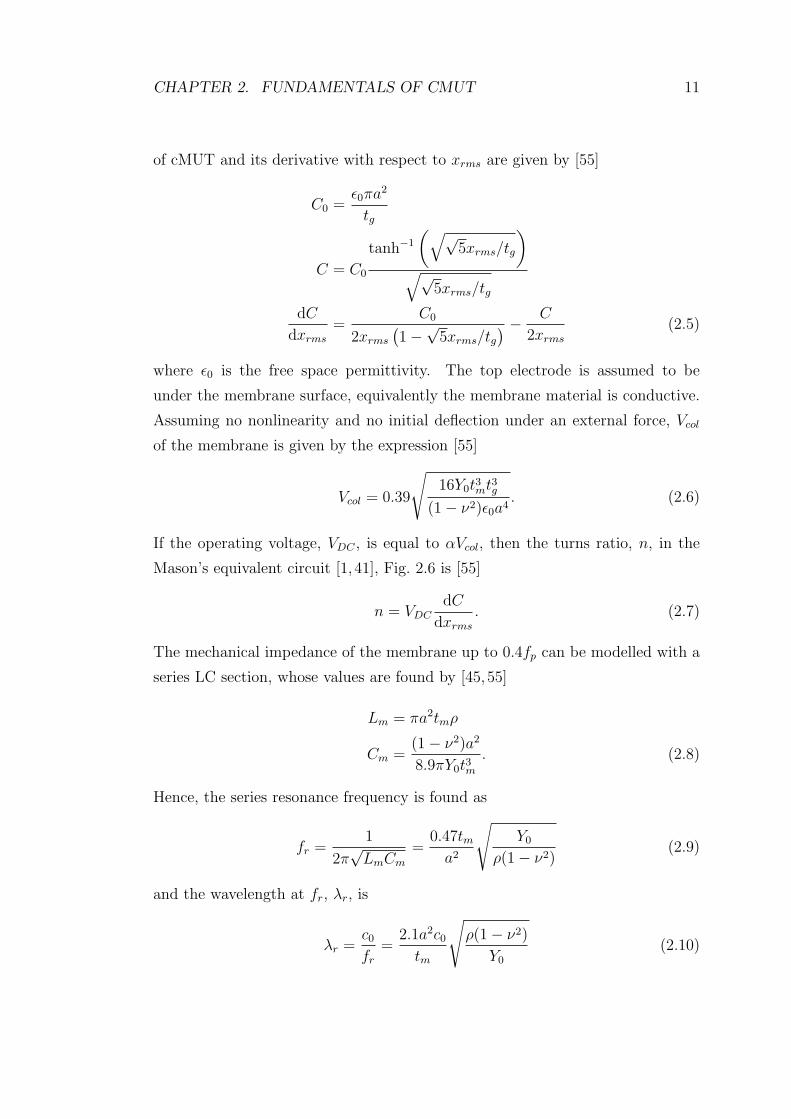
of cMUT and its derivative with respect to xrms are given by [55]
C0 =ε0πa2
tg
C = C0
tanh−1
(√√5xrms/tg
)
√√5xrms/tg
dC
dxrms
=C0
2xrms
(1−√5xrms/tg
) − C
2xrms
(2.5)
where ε0 is the free space permittivity. The top electrode is assumed to be
under the membrane surface, equivalently the membrane material is conductive.
Assuming no nonlinearity and no initial deflection under an external force, Vcol
of the membrane is given by the expression [55]
Vcol = 0.39
√16Y0t3mt3g
(1− ν2)ε0a4. (2.6)
If the operating voltage, VDC , is equal to αVcol, then the turns ratio, n, in the
Mason’s equivalent circuit [1, 41], Fig. 2.6 is [55]
n = VDCdC
dxrms
. (2.7)
The mechanical impedance of the membrane up to 0.4fp can be modelled with a
series LC section, whose values are found by [45,55]
Lm = πa2tmρ
Cm =(1− ν2)a2
8.9πY0t3m. (2.8)
Hence, the series resonance frequency is found as
fr =1
2π√
LmCm
=0.47tm
a2
√Y0
ρ(1− ν2)(2.9)
and the wavelength at fr, λr, is
λr =c0
fr
=2.1a2c0
tm
√ρ(1− ν2)
Y0
(2.10)

CHAPTER 2. FUNDAMENTALS OF CMUT 12
where c0 is the speed of sound in the medium. The radiation impedance of the
cMUT cell is written as [48]
Zr = Rr + iXr = Sρ0c0(Rn + iXn) (2.11)
where ρ0 is the density of the medium. Rn and Xn are the normalized radiation
resistance and reactance.
Figure 2.6: Mason’s equivalent circuit of cMUT. C is the shunt input capacitanceand n is the turns ratio. The membrane impedance up to 0.4fp is modelled witha series LC section. During the reception, cMUT is excited by a force source withan amplitude of PS, where P is the incident pressure field.
The spring softening can be modeled by connecting a capacitor of value −C at
the electrical side in series with the transformer in Mason’s equivalent circuit. To
calculate the deflection under an external force Fext, like atmospheric pressure,
the deflection, xext can be found by solving [55]
Fext = k1xext (2.12)
where k1=1/Cm is the linear spring constant. The spring stiffening can be mod-
eled by using a nonlinear third order spring constant [55]
k3 =−2πY0tm(−896585− 529610ν + 342831ν2)
29645a2(2.13)
with the total mechanical force
F = k1xrms + k3x3rms. (2.14)
However, in cases when the ratio of the membrane thickness to radius and gap
height is high, use of k3 is not enough and a finite element method simulation
must be performed in order to make a correct modeling [66]. Following [67], it is
possible to calculate Vcol when Fext and k3 are present.
CHAPTER 2. FUNDAMENTALS OF CMUT 13
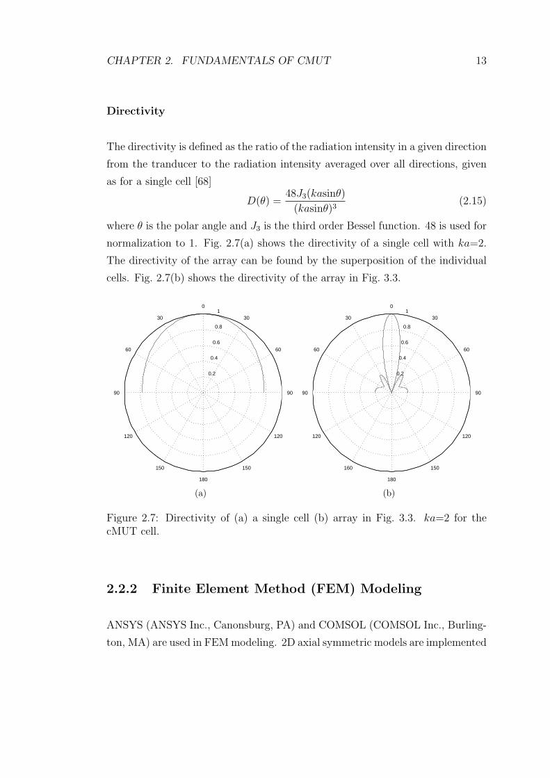
Directivity
The directivity is defined as the ratio of the radiation intensity in a given direction
from the tranducer to the radiation intensity averaged over all directions, given
as for a single cell [68]
D(θ) =48J3(kasinθ)
(kasinθ)3(2.15)
where θ is the polar angle and J3 is the third order Bessel function. 48 is used for
normalization to 1. Fig. 2.7(a) shows the directivity of a single cell with ka=2.
The directivity of the array can be found by the superposition of the individual
cells. Fig. 2.7(b) shows the directivity of the array in Fig. 3.3.
0.2
0.4
0.6
0.8
1
60
120
30
150
0
180
30
150
60
120
90 90
(a)
0.2
0.4
0.6
0.8
1
60
120
30
160
0
180
30
150
60
120
90 90
(b)
Figure 2.7: Directivity of (a) a single cell (b) array in Fig. 3.3. ka=2 for thecMUT cell.
2.2.2 Finite Element Method (FEM) Modeling
ANSYS (ANSYS Inc., Canonsburg, PA) and COMSOL (COMSOL Inc., Burling-
ton, MA) are used in FEM modeling. 2D axial symmetric models are implemented

CHAPTER 2. FUNDAMENTALS OF CMUT 14
using ANSYS 3 to calculate the DC and the AC behaviors with the velocity and
the pressure profiles on the surface of the cMUT membrane [49–51]. The circu-
lar absorbing boundary is 2λ away from the membrane at the lowest operating
frequency and the mesh size is λ/40 at the highest operating frequency. A rigid
baffle is assumed.
3D models are implemented using COMSOL 4. The absorbing boundary is
0.5λ away from the membrane and the mesh size is λ/5 at the operating fre-
quency.
3The membrane, the fluid and the absorbing boundary are modeled using PLANE42,FLUID29 and FLUID129 elements, respectively. Electrostatic elements are modeled usingTRANS126 elements.
4acsld and acpr multiphysics environments are used for the structural and the acousticsolutions, respectively. DC and AC analyses are not implemented.

Chapter 3
RADIATION IMPEDANCE
In this chapter, the radiation impedance of an array of cMUT cells with circular
membranes is presented. First, the radiation impedance of a single cMUT cell
is calculated using its velocity profile. Then, the radiation impedance of array
of cMUT cells is calculated from analytical expressions and compared with those
found from finite element simulations.
3.1 Mechanical Behavior of a Circular cMUT
Membrane
3.1.1 Velocity Profile
The velocity profile on the surface of a circular radiator can be expressed analyt-
ically using a linear combination of functions given by [48,55,69,70]
vn(r) = Vrms
√2n + 1
(1− r2
a2
)n
U(a− r) (3.1)
where U is the unit step function. n =0, 1 and 2 correspond to the velocity
profiles of rigid piston, simply supported and clamped radiators 1, respectively as
1The analytical model of cMUT in Chapter 2 assumes that the cMUT membrane has adisplacement, equivalently velocity profile of (3.1) with n=2.
15

CHAPTER 3. RADIATION IMPEDANCE 16
seen in Fig. 3.1(a). Vrms denotes the rms velocity over the surface of the radiator
given by
Vrms =
√1
S
∫
S
Rev(r)2dS + i
√1
S
∫
S
Imv(r)2dS (3.2)
With this definition, Vrms is a complex number representing the phasor of the
lumped membrane velocity and is non-zero for all velocity profiles.
A radially symmetric velocity profile, v(r), can be written in terms of the
velocity profiles of (3.1) as
v(r) = α0v0(r) + α1v1(r) + · · ·+ αNvN(r)
=N∑
n=0
αnvn(r) (3.3)
The values of the coefficients, αn, are calculated by first equating Vrms in each
vn(r) to Vrms of v(r) resulting in
α20 +
√3α0α1 + · · · = 1
N∑n=0
N∑m=0
√2n + 1
√2m + 1
n + m + 1αnαm = 1 (3.4)
and then using the least mean square algorithm with (3.4) to fit the velocity
distribution to the actual one.
The velocity profile of a cMUT membrane depends on f/fp2. This profile
determined by FEM simulations can be seen in Fig. 3.1(b) for f=0.2fp and can be
approximated using (3.3) with α2=0.94 and α4=0.06. The same figure also shows
the velocity profiles of the membrane at f=0.4fp and f=fp with α2=0.71, α4=0.3
and α2=-2.45, α4=3.06, respectively, approximating the profiles very accurately.
The variation of α2 and α4 is given in Table 3.1 as a function of f/fp.
3.1.2 Radiation Impedance
As mentioned in the previous section, cMUT is a distributed structure. However,
in this work, its displacement and velocity profiles are modeled with a lumped
2The parallel resonance frequency (fp) corresponds to the second circularly symmetric modeof the membrane.

CHAPTER 3. RADIATION IMPEDANCE 17
Table 3.1: Variation of α2 and α4 with respect to f/fp.
f/fp 0 0.1 0.2 0.3 0.4 0.5 0.6 0.7 0.8 0.9 1α2 1 0.99 0.94 0.85 0.71 0.50 0.20 -0.23 -0.86 -1.64 -2.45α4 0 0.012 0.063 0.15 0.30 0.51 0.81 1.22 1.79 2.45 3.06
0 0.1 0.2 0.3 0.4 0.5 0.6 0.7 0.8 0.9 1−1.25
−1
−0.75
−0.5
−0.25
0
r / a
v
n=0
n=1
n=2
(a)
0 0.1 0.2 0.3 0.4 0.5 0.6 0.7 0.8 0.9 1 −1
−0.75
−0.5
−0.25
0
0.25
r / a
v
FEMfrom (3.3)
f=fp
f=0.2fp
f=0.4fp
(b)
Figure 3.1: (a) The velocity profiles of rigid piston, simply supported and clampedradiators normalized to the peak values (b) The velocity profiles of a cMUTmembrane normalized to the peak values determined by FEM simulations atf=0.2fp, 0.4fp and fp. The same profiles approximated using (3.3) with [α2=0.94,α4=0.06], [α2=0.71, α4=0.3] and [α2=-2.45, α4=3.06] are also shown.
velocity variable, vrms, and a function of the radial distance, r. When the square
of this lumped velocity, V , is multiplied with the radiation impedance, Z,
P = V 2Z (3.5)
it gives the total power at the surface of cMUT, P . Hence, the radiation
impedance, Z, of a transducer with a velocity profile, v(r), can be found by
dividing the total power, at the surface of the transducer to the square of the
absolute value of an arbitrary reference velocity, V , [71, 72]
Z =P
|V |2 =
∫S
p(r)v∗(r)dS
|V |2 (3.6)
where p(r) and v∗(r) are the pressure and the complex conjugate of velocity at the
radial distance r. All of the work on modelling the membranes since Mason [41]
employ the average velocity, V =Vave, to represent the reference velocity variable.
CHAPTER 3. RADIATION IMPEDANCE 18
This choice is problematic with some higher mode cMUT velocity profiles, since
it may give V =0 [45] resulting in an infinite radiation impedance. In this thesis,
the reference velocity is chosen to be the root mean square velocity, V =Vrms ,
defined in (3.2). Note that with each choice of the reference velocity, a different
radiation impedance will be obtained and the equivalent circuit variables must
be calculated based on this reference velocity.
For the velocity profile of (3.3), the total radiated power is
P =
∫
S
N∑n=0
N∑m=0
αnαmpn(r)v∗m(r)dS
=N∑
n=0
N∑m=0
αnαmPnm (3.7)
where Pnm is the power generated by vm(r) in the presence of the pressure field,
pn(r) generated by vn(r). Following [70], Pnm can be expressed in a closed form
as
Pnm = Sρ0c0V2rmsA 1−B [F1nm(2ka) + iF2nm(2ka)] (3.8)
where k is the wavenumber and while A and B are constants, F1nm and F2nm
are some functions of ka given in Table 3.2 for n, m=2 and 4. Table 3.3 gives
the small argument approximations of Pnm/Sρ0c0V2rms in (3.8) for ka < 0.25 to
overcome the numerical accuracy problems during the calculation of Bessel and
Struve function terms.
Using (3.3) with n=2 and 4 and combining with (3.6), (3.7) and (3.8), Z is
found as
Z = R + iX =α2
2P22 + 2α2α4P24 + α24P44
|Vrms|2(3.9)
Here, R is the real part and X is the imaginary part of the radiation impedance.
The real part is due to the real power radiated into the medium, whereas the
imaginary part is due to the stored energy in the medium due to the sideways
movements of the medium in the close proximity of the membrane.
The radiation impedance computed from (3.9) and normalized by Sρ0c0 for
piston and clamped radiators (with velociy profiles given by (3.1) for n=0 and
n=2) can be seen in Fig.3.2 as a function of ka. As ka →∞, the mutual effects
vanish and the normalized radiation resistance for both radiators converge to
unity [68, 73]. For the same case, the radiators do not generate reactive power,

CHAPTER 3. RADIATION IMPEDANCE 19
hence the radiation reactances of both radiators approach to zero. The figure
also shows the normalized radiation impedances of three cMUT membranes with
different kpa values as computed from (3.9), where kp is the wavenumber at the
parallel resonance frequency. The velocity profiles corresponding to different ka
values are calculated from Table 3.1 using ka/kpa=f/fp ratios. The frequencies
less than the parallel resonance frequency of the cMUT membrane (ka ≤ kpa) are
considered. cMUTs are similar to the clamped radiators for ka < 0.4kpa. In this
range, the velocity profile of the cMUT membrane follows that of the clamped
radiator. But, for ka > 0.4kpa, deviations from the clamped radiator behavior
occur, especially when kpa is small and the mutual effects are significant. On the
other hand, if kpa is high, the mutual effects are insignificant and R approaches
to that of the clamped radiator.
0 1 2 3 4 5 6 7 8 9 100
0.25
0.5
0.75
1
1.25
1.5
1.75
ka
RSρ0c0
cMUT, kpa=π
cMUT, kpa=2π
cMUT, kpa=4π
Clamped Piston
(a)
0 1 2 3 4 5 6 7 8 9 100
0.25
0.5
0.75
1
1.25
1.5
1.75
ka
XSρ0c0
cMUT, kpa=π
cMUT, kpa=2π
cMUT, kpa=4π
ClampedPiston
(b)
Figure 3.2: The calculated radiation (a) resistance (b) reactance normalized bySρ0c0 of a piston radiator, a clamped radiator and cMUT membranes with kpa=π,2π and 4π. The radiation impedances of the cMUT membranes determined byFEM simulations (circles) are also included. The curves for cMUT membranesare shown for ka ≤ kpa.

CHAPTER 3. RADIATION IMPEDANCE 20
Tab
le3.
2:C
onst
ants
and
funct
ions
use
din
(3.8
).
nm
AB
F1nm
(y)
F2nm
(y)
22
1211·5
(2ka)7
y2J
5(y
)+
2yJ
4(y
)+
3J3(y
)−y
2H
5(y
)−
2yH
4(y
)−
3H3(y
)
−y3/1
6−
y5/7
68+
(2/π
)·(
y4/3
5)+
(2/π
)·(
y6/9
45)
24
3√
57
217·3·
7(2
ka)1
1y
4J
7(y
)+
5y3J
6(y
)+
27y
2J
5(y
)−y
4H
7(y
)−
5y3H
6(y
)−
27y
2H
5(y
)
+10
5yJ
4(y
)+
210J
3(y
)−
35y
3/8
−105
yH
4(y
)−
210H
3(y
)+
(2/π
)·(
2y4)
−y7/(
5.12×
103)−
y9/(
1.84×
105)
+(2
/π)·(
y6/2
7)+
(2/π
)·(
2y8/(
3.47×
103))
44
1223·34
(2ka)1
3y
4J
9(y
)+
4y3J
8(y
)+
18y
2J
7(y
)−y
4H
9(y
)−
4y3H
8(y
)−
18y
2H
7(y
)
+60
yJ
6(y
)+
105J
5(y
)−
7y5/2
56−6
0yH
6(y
)−
105H
5(y
)+
(2/π
)·(
y6/9
9)−y
7/(
6.14×
103)−
y9/(
5.73×
105)
+(2
/π)·(
5y8/(
2.70×
104))
+(2
/π)·(
y10/(
4.05×
105))
−y11/(
3.30×
107)
(2/π
)·(
y12/(
3.45×
107))
Jn
and
Hn
are
the
nth
order
Bes
selan
dStr
uve
funct
ions.

CHAPTER 3. RADIATION IMPEDANCE 21
Table 3.3: Small argument approximations of the real and the imaginary partsof Pnm/Sρ0c0V
2rms in (3.8). (y=ka)
n m Real Imaginary2 2 5y2/72− 5y4/(3.46× 103) 215y/(3.12π × 104)
2 4√
5y2/40−√5y4/(2.30× 103) 222√
5/(1.01π × 107)− 224√
5y3/(1.47π × 109)4 4 9y2/200− 9y4/(1.44× 104) 231y/(2.55π × 109 − 231y3/(1.18π × 1011))
3.2 Radiation Impedance of an Array of cMUT
Cells
cMUTs are used in array configuration. To calculate the radiation impedance
of a cell in an array, the contributions from the neighboring cells must also be
included.
3.2.1 Mutual Radiation Impedance between Two cMUT
Cells
If there are a number of transducers in the close proximity of the each other, one
can define a mutual radiation impedance between them. The mutual radiation
impedance, Zij, between ith and jth transducers is the power generated on the
jth transducer due to the pressure generated by the ith transducer divided by
the product of the reference velocities [72]
Zij =
∫Sj
pi(rj)v∗j (rj)dS
ViV ∗j
i, j = 1, 2 . . . , i 6= j (3.10)
Using (3.3) with n=2 and 4, Zij is found as
Zij = α22Z
22ij + 2α2α4Z
24ij + α2
4Z44ij (3.11)
where Znmij is the mutual radiation impedance between the transducers having
the velocity profiles vn(r) and vm(r) and it can be written as a double infinite
CHAPTER 3. RADIATION IMPEDANCE 22
summation with µ and ν being the summation indices [69]
Znmij =Sρ0c0
2n+mn!m!√
2n + 1√
2m + 1√2kdij(ka)n+m
×∞∑
µ=0
∞∑ν=0
Γ(µ + υ + 1/2)
µ!υ!
(a
dij
)µ+υ
Jµ+n+1(ka)Jυ+m+1(ka)
×[Jµ+υ+ 1
2(kdij) + i(−1)µ+υJ−µ−υ− 1
2(kdij)
] (3.12)
where dij is the distance between ith and jth transducers.
3.2.2 Radiation Impedance of an Array of cMUT Cells
The calculation of the radiation impedance of an array of cMUT cells is demon-
strated with an array, where equal size cells are placed in a hexagonal pattern
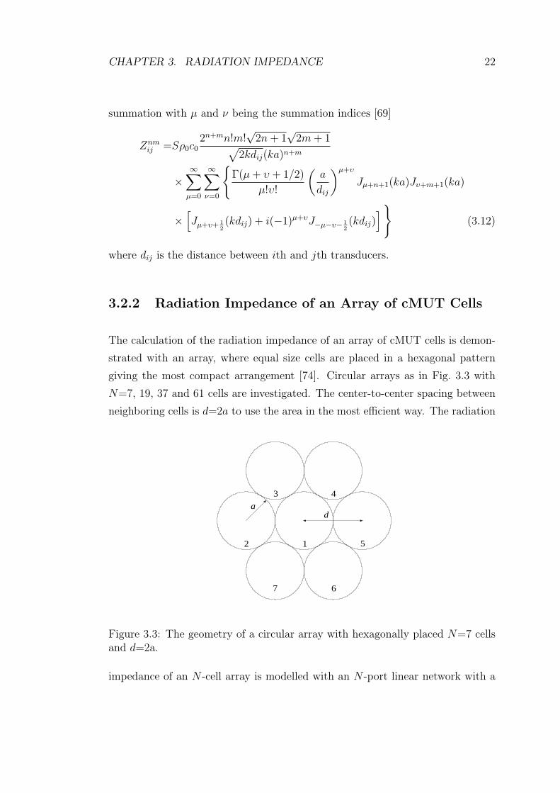
giving the most compact arrangement [74]. Circular arrays as in Fig. 3.3 with
N=7, 19, 37 and 61 cells are investigated. The center-to-center spacing between
neighboring cells is d=2a to use the area in the most efficient way. The radiation
−3 −2 −1 0 1 2 3−3
−2
−1
0
1
2
3
12
3 4
5
67
ad
Figure 3.3: The geometry of a circular array with hexagonally placed N=7 cellsand d=2a.
impedance of an N -cell array is modelled with an N -port linear network with a

CHAPTER 3. RADIATION IMPEDANCE 23
symmetrical N ×N Z-parameter matrix, where the diagonal elements are given
by (3.9) and the off-diagonal elements are found from (3.12):
F1
F2
...
FN
=
Z11 Z12 . . . Z1N
Z12 Z11 . . . Z2N
......
. . ....
Z1N Z2N . . . Z11
V1
V2
...
VN
(3.13)
Here, Fi is the force and Vi is the lumped rms velocity at the ith cell as shown in
Fig. 3.4(a). The LC section models the mechanical impedance of the membrane,
Zm [45,55]. Due to the symmetry, the 7-port network of a 7-cell array in Fig. 3.3
can be simplified to [F1
F2
]= [Z ′]
[V1
6V2
](3.14)
where
(a) (b)
Figure 3.4: The equivalent circuit of the radiation impedance for (a) a generalarray and (b) a circular array with hexagonally placed N=7 cells.
[Z ′] =
[Z11 Z12
Z12 (Z11 + 2Z12 + 2Z24 + Z25)/6
](3.15)
since Z12=Z23=Z27 and Z24=Z26. The resulting equivalent circuit is depicted in
Fig. 3.4(b). Since the radiation impedance of each cell is different, a representative
radiation impedance, Zr, of a single cell is defined as
Zr = NF
V− Zm = Rr + iXr (3.16)

CHAPTER 3. RADIATION IMPEDANCE 24
0 1 2 3 4 5 6 7 8 9 100
0.25
0.5
0.75
1
1.25
1.5
1.75
2
2.25
2.5
kd
Rr
Sρ0c0
Piston, N=19
cMUT, N=61
N=37
N=19
N=7
(a)
0 1 2 3 4 5 6 7 8 9 100
0.25
0.5
0.75
1
1.25
1.5
1.75
2
2.25
2.5
kd
Rr
Sρ0c0
cMUT, N=61
N=37
N=19
N=7
Piston, N=19
(b)
Figure 3.5: The representative radiation resistance, Rr, normalized by Sρ0c0 ofa single cMUT cell in N=7, 19, 37 and 61 element arrays in comparison to a cellin N=19 element piston array all with a/d=0.5 as a function of kd for a cMUTcell with (a) kpa=2π and (b) kpa=4π. The representative radiation resistancedetermined by FEM simulations (circles) are also shown.
where F and V are as shown in Fig. 3.4.
Fig. 3.5 shows the representative radiation resistance of a single cell normal-
ized by Sρ0c0 in various arrays as a function of kd for cMUT cells with kpa=2π
and 4π. For kd < 5, Rr of the cMUT cell shows a behavior similar to that of
an array of pistons [62] except for the vertical scale. As kd increases, the posi-
tive loading on the each cell increases and Rr becomes maximum around kd=7.5,
where the loading reaches an optimum point [73]. As N increases, the maximum
value of the radiation resistance, Rmax , also increases, while the corresponding
kd value, kdopt, is not significantly affected. On the other hand, as kd → ∞,
the mutual effects vanish and normalized value of Rr approaches to that of an
individual cell. Note that for thin membranes with kpa < 3.7, kdopt=7.5 point
is beyond the parallel resonance frequency, hence such a maximum will not be
present.
The variation of Rmax and kdopt is investigated by changing the distance be-
tween the cells for an array with kpa=4π. The first peak in the radiation resis-
tance and the corresponding kd value are taken as Rmax and kdopt, respectively.
As depicted in Fig. 3.6, a/d=0.42 and kdopt=7.68 define the optimum separation
for N=19. For example, at f=100 kHz, this maximum for an airborne cMUT
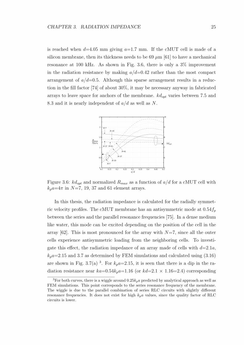
CHAPTER 3. RADIATION IMPEDANCE 25
is reached when d=4.05 mm giving a=1.7 mm. If the cMUT cell is made of a
silicon membrane, then its thickness needs to be 69 µm [61] to have a mechanical
resonance at 100 kHz. As shown in Fig. 3.6, there is only a 3% improvement
in the radiation resistance by making a/d=0.42 rather than the most compact
arrangement of a/d=0.5. Although this sparse arrangement results in a reduc-
tion in the fill factor [74] of about 30%, it may be necessary anyway in fabricated
arrays to leave space for anchors of the membrane. kdopt varies between 7.5 and
8.3 and it is nearly independent of a/d as well as N .
0.1 0.15 0.2 0.25 0.3 0.35 0.4 0.45 0.5 0
0.5
1
1.5
2
2.5
a/d
Rmax
Sρ0c0
5
6
7
8
9
10
kdopt
N=61
N=61
N=37
N=37
N=19
N=19
N=7
N=7
Figure 3.6: kdopt and normalized Rmax as a function of a/d for a cMUT cell withkpa=4π in N=7, 19, 37 and 61 element arrays.
In this thesis, the radiation impedance is calculated for the radially symmet-
ric velocity profiles. The cMUT membrane has an antisymmetric mode at 0.54fp
between the series and the parallel resonance frequencies [75]. In a dense medium
like water, this mode can be excited depending on the position of the cell in the
array [62]. This is most pronounced for the array with N=7, since all the outer
cells experience antisymmetric loading from the neighboring cells. To investi-
gate this effect, the radiation impedance of an array made of cells with d=2.1a,
kpa=2.15 and 3.7 as determined by FEM simulations and calculated using (3.16)
are shown in Fig. 3.7(a) 3. For kpa=2.15, it is seen that there is a dip in the ra-
diation resistance near ka=0.54kpa=1.16 (or kd=2.1 × 1.16=2.4) corresponding
3For both curves, there is a wiggle around 0.25kpa predicted by analytical approach as well asFEM simulations. This point corresponds to the series resonance frequency of the membrane.The wiggle is due to the parallel combination of series RLC circuits with slightly differentresonance frequencies. It does not exist for high kpa values, since the quality factor of RLCcircuits is lower.
CHAPTER 3. RADIATION IMPEDANCE 26
0 1 2 3 4 5 6 7 80
0.1
0.2
0.3
0.4
0.5
0.6
0.7
0.8
0.9
1
kd
Rr
Sρ0c0
kpa=2.15
kpa=3.7
(a)−2
−1
0
1
2
−2
−1
0
1
2
−10
−5
0
5
10
(b)
Figure 3.7: (a) The representative radiation resistance normalized by Sρ0c0 of asingle cMUT cell in N=7 element array in water for a cell with d=2.1a, kpa=2.15and 3.7. The representative radiation resistance determined by FEM simulations(circles) are also depicted. Note that the kpa=2.15 curve does not have thekdopt=7.5 peak. The discrepancy between FEM simulations and analytic curve isdue to the presence of antisymmetric mode. (b) FEM computed velocity profileof the cells showing the excitation of antisymmetric mode at the outer cells forkpa=2.15 and kd=2.4.
to the antisymmetric mode as determined from FEM simulations, which is not
predicted by (3.16). The velocity profiles of the cells showing the excitation of an-
tisymmetric mode at this frequency can be seen in Fig. 3.7(b). As kpa increases,
this effect is less pronounced. For kpa=3.7, the dip is still present near kd=2.1
× 0.54kpa=4.2, but it is smaller. As seen in Fig. 3.5, the dip is nonexistent in
thicker membranes with kpa=2π or kpa=4π. Similarly, such dips are not present
for airborne transducer arrays, since antisymmetric modes are not excited.
Chapter 4
AIRBORNE cMUTs
In this chapter, the performance of a cMUT array having a circular shape oper-
ating in air is optimized by increasing the radiation resistance of the array. This
is achieved by choosing the size of the cMUT membranes and their placement
within the array. The proposed approach improves the bandwidth as well as the
transmitted power of the array. First, the radiation resistance of a cMUT array
having a circular shape is optimized. Then, the quality factors of the various
cMUT arrays are calculated. The transmit and the receive performances are
calculated assuming the conventional operating conditions. The results are pre-
sented as normalized design graphs, which make them possible to be used for an
arbitrary device dimensions and a material property. Design examples are given
to demonstrate the use of these graphs.
4.1 Performance Figures
The cMUT cell operates around its series resonance frequency (fr) in air [1,12,63].
In this section, a circular array, where the cells are placed in a hexagonal pattern,
as depicted in Fig. 4.1 is investigated. The effective radius of the array, A, is
equal to
A = a√
N/fF with fF = (2π/√
3)(a/d)2 (4.1)
27

CHAPTER 4. AIRBORNE CMUTS 28
The effects of the parameters, a, A and d on the transmit and the receive per-
formances of the cMUT are investigated while the other parameters are kept
constant. A noise analysis is provided to determine the noise figure of the sys-
tem including the receiver electronics. The membrane material is assumed to
be silicon. Analytical expressions are presented for each performance figure. As
a is changed, tm and tg are adjusted to keep the resonance frequency and the
collapse voltage constant. In order to keep A constant at the specified value, N
is adjusted as an integer variable. Since the acoustic loading is low,compared to
the mechanical impedance of the membrane, the effect of the radiation reactance
is ignored. The results are displayed on normalized graphs.
−6 −4 −2 0 2 4 6−6
−4
−2
0
2
4
6
a d
A
Figure 4.1: The geometry of a circular array with hexagonally placed N=19 cells.
4.1.1 Radiation Resistance
In the previous chapter, it is shown that the radiation resistance (Rr) of a cMUT
cell in an array is a strong function of d [48]. It is maximized, when d is around
1.25λr for the most compact arrangement (d=2a). On the other hand, such an
arrangement requires relatively large radius cells with relatively thick membranes
to meet the resonance frequency requirement. However, a smaller cell radius
would allow a thinner membrane with a potentially better bandwidth [63]. In

CHAPTER 4. AIRBORNE CMUTS 29
order to increase Rr for a smaller cell radius, d is made larger than 2a to get a
sparse arrangement of the cells [64, 73, 76]. Fig. 4.2 shows the normalized radia-
tion resistance (Rn) of a single cell in various arrays made of different cMUTs as
a function of d/a and the variation of the optimum separation to maximize Rn,
dopt, and its value, Rmax, with respect to a/λr.
As shown in Fig. 4.2(a), Rn can be maximized for a lower a value as d/a is
increased [48, 64, 76]. At these points, the net loading on each cMUT is maxi-
mized [48, 64, 73, 76]. As A is increased, the maximum value of Rn for a given
cMUT cell also increases. Note that for a membrane with a/λr=0.3 in an array
with A/λr=3, Rn is more than three times higher when d/a=2.8 compared to the
most compact arrangement of d/a=2.
2 2.1 2.2 2.3 2.4 2.5 2.6 2.7 2.8 2.9 3 0
0.25
0.5
0.75
1
1.25
1.5
1.75
2
2.25
2.5
2.75
d / a
Rn
a/λr=0.5 a/λ
r=0.4
a/λr=0.3
A/λr=3
A/λr=4
A/λr=5
A/λr=6
(a)
0
0.125
0.25
0.375
0.5
0.625
0.75
0.875
1
1.125
1.25
1.375
a / λr
d / λr
0.3 0.35 0.4 0.45 0.5 0.55 0.6 0
0.25
0.5
0.75
1
1.25
1.5
1.75
2
2.25
2.5
2.75
Rnm
ax
A/λr=3
A/λr=4
A/λr=5
A/λr=6
(b)
Figure 4.2: (a) The normalized radiation resistance (Rn) of a single cell in variousarrays as a function of d/a. (b) The change of the optimum separation (dopt) andthe maximum normalized radiation resistance (Rmax) as a function of a/λr.
4.1.2 Q Factor
In air, Q is determined by the series RLC section at the mechanical side of the
Mason’s equivalent circuit [63]. Hence
Q =2πfrLm
Rr
(4.2)
CHAPTER 4. AIRBORNE CMUTS 30
Using (2.8) and (2.11) and expressing the membrane thickness (tm) in terms of a
and λr (2.10), Q (4.2) can be rewritten as
Q =23.8c0ρ
ρ0
√ρ(1− ν2)
Y0
a2
λ2rRn
(4.3)
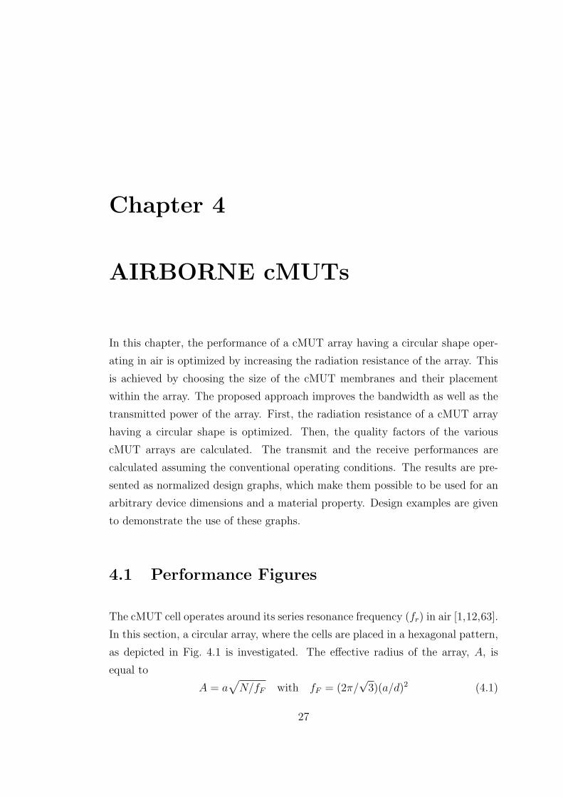
As seen from (4.3), a smaller a is desirable since it reduces Q. On the other hand,
a higher Rn also reduces Q by increasing the loading on the cell. Fig. 4.3 shows
Q of various arrays made of different cMUTs as a function of d/a.
As depicted in Fig. 4.3, Q of each array has a minimum at the point, where
Rn is maximized. For the most compact arrangement, Q for all devices are above
150, however with a sparse arrangement, it is possible to obtain Q below 50
without introducing any lossy elements to the system. For a fixed cell size, Q is
lower when the cell is in a larger array due to increased Rn.
2 2.1 2.2 2.3 2.4 2.5 2.6 2.7 2.8 2.9 3 0
50
100
150
200
250
300
350
400
d / a
Q
a/λr=0.5
a/λr=0.4
a/λr=0.3
A/λr=3
A/λr=4
A/λr=5
A/λr=6
Figure 4.3: Q of various arrays as a function of d/a.
4.1.3 Transmit Mode
To maximize the power transferred to the medium, cMUT is driven such that the
membrane swings the entire stable gap height (the allowed swing range of the
membrane without collapsing), which is 0.46tg for the peak displacement [55].
The velocity of the membrane will be sinusoidal with frequency fr, since Q is
relatively high [77]. Then, rms velocity of the membrane is [55, 64,76]
vrms =2πfrxrms√
2=
0.46πtgfr√10
(4.4)

CHAPTER 4. AIRBORNE CMUTS 31
If tg is expressed in terms of Vcol from (2.6) and tm is eliminated using (2.10), the
average output power from a single cMUT cell is
Pave = v2rmsRr =
0.045ρ0c0
ρ
(Y0ε
20
(1− ν2)
)1/3
a2/3V4/3col Rn (4.5)
and the average output power from the array will be N times of (4.5). Then
Pave = Nv2rmsRr =
0.16ρ0c0
ρ
(Y0ε
20
(1− ν2)
)1/3a2/3A2V
4/3col Rn
d2(4.6)
Fig. 4.4 shows the average output power normalized by λr and Vcol per unit area
of various arrays made of different cMUTs as a function of d/a. It is seen that
Pave is maximized, when Rn is maximized (4.6). Note that as d/a increases, N
decreases. Consequently for a/λr=0.3, Pave is only 1.5 times higher, although the
increase in Rn is more than 3 times compared to the most compact arrangement.
2 2.1 2.2 2.3 2.4 2.5 2.6 2.7 2.8 2.9 3 0
1
2
3
4
5
6
7
d / a
Pav
e / (λ
r2/3 V
col
4/3 )
(µW
/ (m
2/3 V
4/3 ))
a/λr=0.5
a/λr=0.4 a/λ
r=0.3
A/λr=3
A/λr=4
A/λr=5
A/λr=6
Figure 4.4: The average output power normalized by λr and Vcol per unit area ofvarious arrays as a function of d/a.
4.1.4 Receive Mode
The receive performance of a transducer is specified by its open-circuit voltage,
Voc, together with the input resistance, Rin, and the capacitance, Cin, hence the
input impedance, Zin, is given by the parallel combination of Rin and Cin. In
order to calculate these parameters, C for Cin (2.5) and dC/dxrms for n hence
CHAPTER 4. AIRBORNE CMUTS 32
Rin (2.5, 2.7) are required. If a normalized displacement such that x=xrms/tg is
defined [78], then x will depend only on the ratio of the operating voltage to the
collapse voltage (α) [55,78]. Using (2.5), C and dC/dxrms are rewritten as
C =ε0πa2
tg
tanh−1(√√
5x)
√√5x
=ε0πa2
tgfc(α)
dC
dxrms
=ε0πa2
2t2g
(1
x(1−√5x
) −√√
5x
x√√
5x
)
=ε0πa2
2t2gfdC(α) (4.7)
The Mason’s equivalent circuit in Fig. 2.6 is used to calculate the receive mode
parameters. cMUT is excited by a force source with an amplitude of PS where P
is the incident pressure field. α is assumed to be 0.9 giving fc=1.11 and fdC=2.90.
Voc is given by the voltage division between the shunt input capacitance C and the
remaining of the network. For the typical device dimensions and the operating
frequencies in air, which is in the 1 mm and 100 kHz range, C shows a high
impedance compared to the rest of the network and can be ignored. Then
Voc
P=
S
n=
0.095c20
ρ
(Y0
ε0(1− ν2)
)1/3λ2
rV1/3col
a4/3(4.8)
which is independent of Rn. The material dependent part is equal to 1.2 ×10⁸ (V 2/3 m4/3)/N. The input resistance will be equal to the radiation resistance
referred to the electrical side, whereas the input capacitance will be the shunt
input capacitance. Then, Rin and Cin of a single cell are
Rin =Rr
n2=
0.0029ρ0
c30ρ
2
(Y 2
0
ε20(1− ν2)2
)1/3λ4
rV2/3col Rn
a14/3
Cin = C = 1.22ρ0ε4/30
(Y0
ρ3(1− ν2)
)1/6a8/3
λrV2/3col
(4.9)
CHAPTER 4. AIRBORNE CMUTS 33
and since cMUTs in an array are connected in parallel, Rin and Cin of the array
are
Rin =Rr
Nn2=
0.0008ρ0
c30ρ
2
(Y 2
0
ε20(1− ν2)2
)1/3d2λ4
rV2/3col Rn
a14/3A2
Cin = NC = 4.45ρ0ε4/30
(Y0
ρ3(1− ν2)
)1/6a8/3A2
d2λrV2/3col
(4.10)
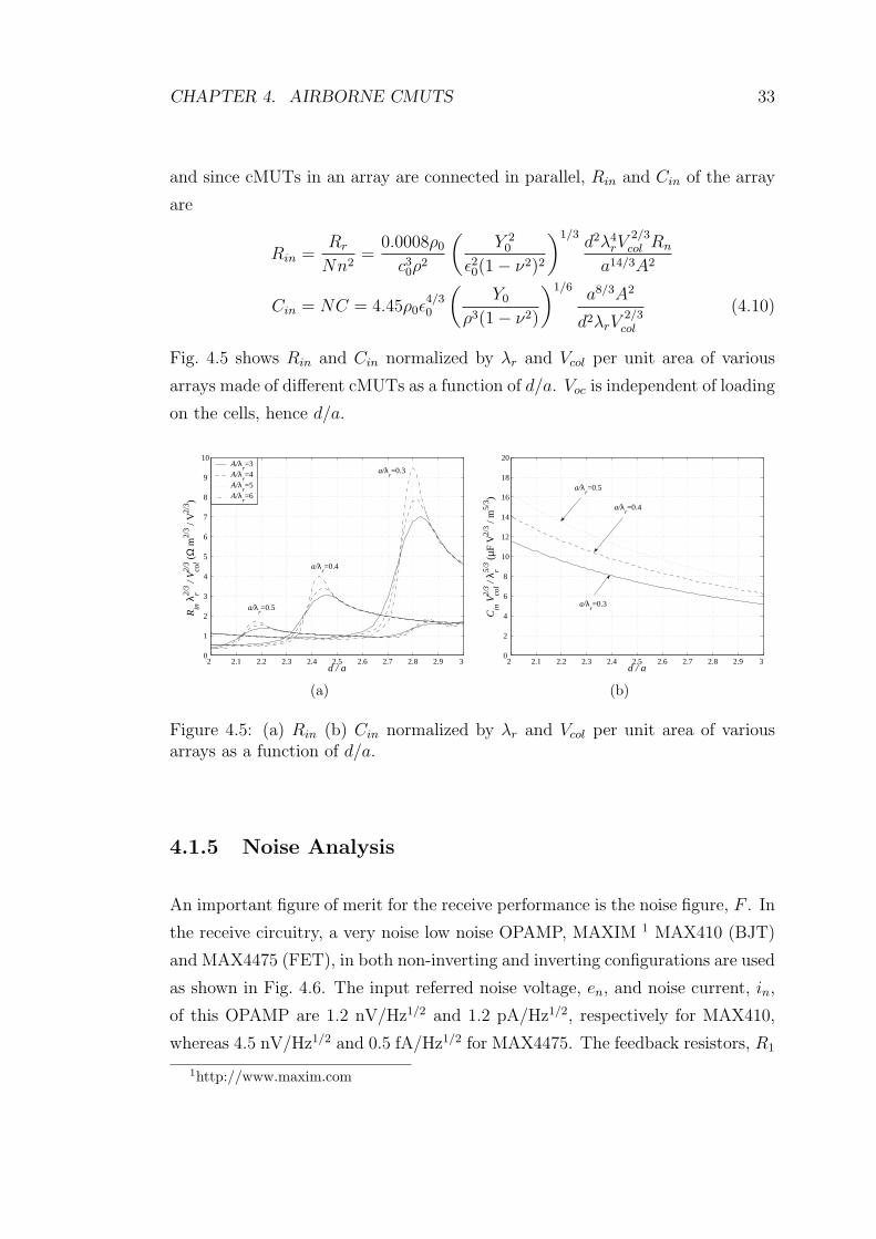
Fig. 4.5 shows Rin and Cin normalized by λr and Vcol per unit area of various
arrays made of different cMUTs as a function of d/a. Voc is independent of loading
on the cells, hence d/a.
2 2.1 2.2 2.3 2.4 2.5 2.6 2.7 2.8 2.9 3 0
1
2
3
4
5
6
7
8
9
10
d / a
Rin
λr2/
3 / V
col
2/3 (
Ω m
2/3 /
V2/
3 )
a/λr=0.5
a/λr=0.4
a/λr=0.3
A/λr=3
A/λr=4
A/λr=5
A/λr=6
(a)
2 2.1 2.2 2.3 2.4 2.5 2.6 2.7 2.8 2.9 3 0
2
4
6
8
10
12
14
16
18
20
d / a
Cin
Vco
l2/
3 / λ r5/
3 (µF
V2/
3 / m
5/3 )
a/λr=0.5
a/λr=0.4
a/λr=0.3
(b)
Figure 4.5: (a) Rin (b) Cin normalized by λr and Vcol per unit area of variousarrays as a function of d/a.
4.1.5 Noise Analysis
An important figure of merit for the receive performance is the noise figure, F . In
the receive circuitry, a very noise low noise OPAMP, MAXIM 1 MAX410 (BJT)
and MAX4475 (FET), in both non-inverting and inverting configurations are used
as shown in Fig. 4.6. The input referred noise voltage, en, and noise current, in,
of this OPAMP are 1.2 nV/Hz1/2 and 1.2 pA/Hz1/2, respectively for MAX410,
whereas 4.5 nV/Hz1/2 and 0.5 fA/Hz1/2 for MAX4475. The feedback resistors, R1
1http://www.maxim.com

CHAPTER 4. AIRBORNE CMUTS 34
and R2 are chosen as 1 kΩ and 10 kΩ. The noise contributions from the resistors
can be decreased by connecting parallel capacitors, C1 and C2 with values of -100j
and -1000j Ω at the operating frequency. Zopt is determined from ANSOFTTM
simulations. For MAX410, Zopt is 3.5 and 2.7 kΩ giving F of 2.55 and 3.86 dB for
the non-inverting and the inverting configurations without the capacitors. With
the capacitors, Zopt = Ropt + iXopt is 1289 + j 90 and 524 + j 522 Ω giving F of
0.91 and 1.41 dB. For MAX4475, Zopt is 11.8 M and 4.8 kΩ giving F of 0.0016
and 4.1 dB for the non-inverting and the inverting configurations without the
capacitors. With the capacitors, Zopt = Ropt + iXopt is 9M + j 409 and 4.3 + j
1.1 kΩ giving F of 0.0016 and 3.17 dB. Since the optimum source impedance to
minimize the noise figure, Zopt, is below a few kΩs, which is comparable to Rin, a
BJT choice is preferable. Fig. 4.7 shows F of the receiver circuitries as the source
resistance, Rs, is changed.
(a) (b)
Figure 4.6: The receiver circuitry used in the calculations of the noise figure,OPAMP with (a) non-inverting (b) inverting configurations.
Minimizing the noise figure depends on the termination of the receiver ampli-
fier with the optimum source resistance. Note that as the distance between the
cells increases, due to the reduced fill factor, the intercepted input signal power
decreases. This eventually decreases the noise figure. Table 4.1 shows the reduc-
tion in F with respect to d/a. Also if Rin of cMUT is lower compared to the real
part of Ropt, it is possible to decrease F by clustering the cells [64], decreasing
the number of the cells connected to the receiver amplifier.

CHAPTER 4. AIRBORNE CMUTS 35
101
102
103
104
105
0
1
2
3
4
5
6
7
8
9
10
Rs
F (dB)
Non−inverting without C
Non−inverting with C
Inverting without C
Inverting with C
(a)
101
102
103
104
105
0
1
2
3
4
5
6
7
8
9
10
Rs
F (dB)
Non−inverting without C
Non−inverting with C Inverting without C
Inverting with C
(b)
Figure 4.7: F of various receiver circuitries as a function of Rs. (a) BJT (b) FETOPAMP
Table 4.1: Reduction in noise figure (dB).
d/a 2 2.1 2.2 2.3 2.4 2.5 2.6 2.7 2.8 2.9 3F 0.41 0.81 1.25 1.6 2 2.3 2.68 3.01 3.28 3.57 3.87
4.2 Design Examples
Let’s demonstrate the use of the normalized graphs with an example. Suppose
that a cMUT array operating at 100 kHz (λr=3.3 mm) is required and the avail-
able area is 12.4 cm2, equivalently A=19.9 mm=6λr. The radius of the sin-
gle cell, a is chosen to be 0.99 mm=0.3λr and corresponding tm=23.5 µm from
(2.10). Two designs are provided. In the first design, the choice of d/a=2 gives
N = (2π/√
3)(62/0.3222)=362 from (4.1). In the second design, d/a=2.8 is cho-
sen and results in N=185. From Fig. 4.2(a), it is found that Rn=0.5 and 2.25 for
d/a=2 and 2.8, respectively. Then, Rr = π×0.99mm2×1.27×331×0.5=647 kg/s
for the former one from (2.11) and Rr=2900 kg/s for the latter one. This shows
that cMUTs in the sparse array are better loaded by air.
Q factors of the designs can be determined from Fig. 4.3. For the first design
(d/a=2), Q is equal to 160 giving a bandwidth of 625 Hz. For the second design
(d/a=2.8), Q is equal to 45, with a bandwidth of 2.2 kHz.
Let the available bias voltage be 250 V, which is chosen to be Vcol giving

CHAPTER 4. AIRBORNE CMUTS 36
tg=7.2 µm from (2.6). From Fig. 4.4, the normalized output powers are read as
2.7 and 5.8 µW/(m2/3V4/3). Note that these values are for a unit circular area.
Keeping in mind this, actual powers are Pave = 2.7µW×3.3mm2/3× 2504/3× π×62=10.7 mW and 23 mW for the first and the second designs, respectively. Voc is
calculated from (4.8) as 70 mV. Whereas, Rin is calculated as 17 and 150 Ω and
Cin is 1.5 nF and 0.78 nF.
For the receiver circuitry, let’s choose non-inverting amplifier with capacitors,
which has the lowest noise figure. F is read as 4.9 and 3.04 dB, respectively. After
the correction in Table 4.1 is made, F is 4.9 and 6.32 dB. Suppose that, there are
four available receiver circuitries and each array is divided into four equal parts
(clustering). Then, each part has an input resistance of 280 and 600 Ω. Then,
F of each configuration will be 2.35 and 4.44 dB. Note that reduction in the fill
factor severely degrades F .
Table 4.2: The comparison of the most compact and the sparse arrangements.
N Rr Q Pave Voc Rin Cin F(kg/s) (mW) (mV) (Ω) (nF) (dB)
d/a=2 362 647 160 10.7 70 17 1.5 4.9d/a=2.8 185 2900 45 23 70 150 0.78 6.32

Chapter 5
CONCLUSION
Capacitive micromachined ultrasonic transducers (cMUTs) are competitive to
the piezoelectric transducers due to the compatibility with silicon IC technology.
They have a wider bandwidth with a lower transmit power and a receive sensitiv-
ity. But they are not on the medical imaging market, which seems to be the most
profitable application area. In order to be commercialized, they should overcome
these drawbacks, on which the active research is going on. An alternative way
will be the use of cMUTs in areas, where the piezoelectric transducers perform
poorly or cannot work. In this thesis, the latter approach is followed to design
wide band and highly efficient airborne transducers with high output power.
In the first part, the radiation impedance of a cMUT with a circular clamped
membrane is calculated up to its parallel resonance frequency. The velocity profile
of the membrane is written as a superposition of analytic velocity profiles whose
weights are dependent on frequency. These profiles are used to calculate the in-
dividual and the mutual radiation impedances from given expressions. Radiation
impedance of any combination of cells can be found by considering only two cells
at a time. Circular arrays are investigated to find the radiation resistances. It
is found that the radiation resistance is a strong function of the separation of
the cells. The center-to-center separation of the cells needs to be around 1.25λ
(kd=7.8) for a high radiation resistance. Note that the optimum cell separation
may require a cMUT cell with an unusually large radius. With an increased
37

CHAPTER 5. CONCLUSION 38
radius, the thickness of the membrane must also be increased to preserve the
resonance at the operating frequency. In this case, the gap height may have to
be reduced to keep the bias voltage at an acceptable level, since an increased
membrane thickness implies a higher bias voltage. The model is perfectly valid
for airborne applications. However, for thin membranes with kpa < 4, the model
may fail in water immersion around the antisymmetric mode.
In the second part, the bandwidth of a cMUT array operating in air with a
fixed area is optimized. The contradictory condition on the thickness of the mem-
brane between the bandwidth and the output power is overcome by maximizing
the radiation resistance with a proper choice of the cell size and the distance
between the cells. It is shown that the thin membranes can have radiation re-
sistances close to the maximum, which the thick membranes have. The Mason’s
equivalent circuit is used to measure cMUT performance. Analytical expressions
are given for different operating modes. In order to make a fair comparison, the
operating frequency and the collapse voltage of the devices are kept constant.
The improvement in the bandwidth and the transmit power can be as high as
three and one and a half times, respectively. The open circuit voltage is found to
be independent of the radiation resistance. In order to calculate the noise figure
of the system, a state of the art low noise OPAMP is used in the receiver circuitry.
Two amplifier configurations are investigated. It is shown that noise figure close
to the minimum noise figure of the receiver circuitry can be achieved by changing
the number of the cells connected to the receiver, equivalently adjusting the in-
put resistance. All results are presented as normalized design graphs, which are
suited for the design of arbitrary size cMUTs.
The optimization process is suitable for the airborne applications, where the
membrane impedance is much higher than the medium impedance. The increase
in the bandwidth and the transmit power are proportional to the increase in the
radiation resistance, since the bandwidth of the optimized radiation resistance is
wider than the actual device bandwidth. On the other hand, in immersion ap-
plications, the membrane impedance is much lower than the medium impedance
resulting in a wide bandwidth and this process is not suited except that the trans-
ducer will be only used for single frequency continuous wave excitation for high
power transmission. It must be noted that since the acoustic impedance of the

CHAPTER 5. CONCLUSION 39
immersion medium is high, the transmission process may result in the excitation
of the antisymmetric modes in some cells of the array. This will be dominant
especially in small symmetric shape arrays.
The future work for cMUTs must be to increase the transmit power and
the sensitivity in order to compete with the piezoelectric transducers. One ap-
proach will be cMUTs to work at the collapse region with the optimized con-
figuration [79], which seems to be the most promising way. The optimization
includes the arrangement of the electrodes for the maximum transmit power and
the receive voltage. It is possible to operate cMUTs beyond the maximum sta-
ble deflection point in conventional regime overcoming the collapse. There are
several approaches used in MEMS devices also applicable to cMUTs. These are
connecting a capacitor in series with the cMUT [80, 81], driving the cMUT with
a current pulse [82] and use of a resonant drive [83, 84]. The leveraged bending
approach [85] is already employed to cMUTs and very good results are obtained.
This shows that the above methods will also increase the cMUT performance
with a high probability.
Bibliography
[1] M. I. Haller and B. T. Khuri-Yakub, “A surface micromachined electrostatic
ultrasonic air transducer,” IEEE Trans. Ultrason., Ferroelect., Freq. Contr.,
vol. 43, pp. 1–6, 1996.
[2] I. Ladabaum, X. Jin, H. T. Soh, A. Atalar, and B. T. Khuri-Yakub, “Surface
micromachined capacitive ultrasonic transducers,” IEEE Trans. Ultrason.,
Ferroelect., Freq. Contr., vol. 45, pp. 678–690, 1998.
[3] X. Jin, I. Ladabaum, and B. T. Khuri-Yakub, “The microfabrication of ca-
pacitive ultrasonic transducers,” IEEE J. Microelectromech. Syst., vol. 7, pp.
295–302, 1998.
[4] Y. Huang, A. S. Ergun, E. Hæggstrom, M. H. Badi, and B. T. Khuri-Yakub,
“Fabricating capacitive micromachined ultrasonic transducers with wafer-
bonding technology,” IEEE J. Microelectromech. Syst., vol. 12, pp. 128–137,
2003.
[5] J. Knight, J. McLean, and F. L. Degertekin, “Low temperature fabrica-
tion of immersion capacitive micromachined ultrasonic transducers on silicon
and dielectric substrates,” IEEE Trans. Ultrason., Ferroelect., Freq. Contr.,
vol. 51, pp. 1324–1333, 2004.
[6] A. S. Ergun, Y. Huang, X. Zhuang, O. Oralkan, G. G. Yaralıoglu, and B. T.
Khuri-Yakub, “Capacitive micromachined ultrasonic transducers: fabrica-
tion technology,” IEEE Trans. Ultrason., Ferroelect., Freq. Contr., vol. 52,
pp. 2242–2258, 2005.
40
BIBLIOGRAPHY 41
[7] J. Johnson, O. Oralkan, U. Demirci, S. Ergun, M. Karaman, and B. T.
Khuri-Yakub, “Medical imaging using capacitive micromachined ultrasonic
transducer arrays,” Ultrasonics, vol. 40, pp. 471–476, 2002.
[8] F. L. Degertekin, M. Karaman, and R. O. Guldiken, “Forward-looking IVUS
imaging using an annular-ring CMUT array,” in Proc. IEEE Ultrason. Symp.,
2005, pp. 129–132.
[9] C. Daft, P. Wagner, B. Bymaster, S. Panda, K. Patel, and I. Ladabaum,
“cMUTs and electronics for 2D and 3D imaging, monolithic integration, in-
handle chip sets and system implications,” in Proc. IEEE Ultrason. Symp.,
2005, pp. 463–474.
[10] G. Caliano, R. Carotenuto, E. Cianci, V. Foglietti, A. Caronti, A. Iual, and
M. Pappalardo, “Design, fabrication and characterization of a capacitve mi-
cromachined ultrasonic probe for medical imaging,” IEEE Trans. Ultrason.,
Ferroelect., Freq. Contr., vol. 52, pp. 2259–2269, 2005.
[11] S. Olcum, M. N. Senlik, H. K. Oguz, A. Bozkurt, A. Atalar, and H. Koymen,
“A wafer bonded capacitive micromachined underwater transducer,” in Proc.
IEEE Ultrason. Symp., 2009, to be published.
[12] I. O. Wygant, M. Kupnik, J. C. Windsor, W. M. Wright, M. S. Wochner,
G. G. Yaralioglu, M. F. Hamilton, and B. T. Khuri-Yakub, “50 kHz capac-
itive micromachined ultrasonic transducers for generation of highly direc-
tional sound with parametric arrays,” IEEE Trans. Ultrason., Ferroelect.,
Freq. Contr., vol. 56, pp. 193–203, 2009.
[13] S. T. Hansen, A. S. Ergun, W. Liou, B. A. Auld, and B. T. Khuri-Yakub,
“Wideband micromachined capacitive microphones with radio frequency de-
tection,” J. Acoust. Soc. Am., vol. 116, pp. 828–842, 2004.
[14] N. A. Hall, B. Bicen, M. K. Jeelani, W. Lee, S. Qureshi, and F. L. Degertekin,
“Micromachined microphones with diffraction-based optical displacement
detection,” J. Acoust. Soc. Am., vol. 118, pp. 3000–3009, 2005.
BIBLIOGRAPHY 42
[15] I. Ladabaum, X. C. Jin, and B. T. Khuri-Yakub, “Air coupled through
transmission of aluminum and other recent results using MUTs,” in Proc.
IEEE Ultrason. Symp., 1997, pp. 983–986.
[16] I. J. Oppenheim, A. Jain, and D. W. Greve, “MEMS ultrasonic transducers
for the testing of solids,” IEEE Trans. Ultrason., Ferroelect., Freq. Contr.,
vol. 50, pp. 305–311, 2003.
[17] J. McLean and F. L. Degertekin, “Capacitive micromachined ultrasonic
transducers with asymmetric membranes for microfluidic applications,” in
Proc. IEEE Ultrason. Symp., 2001, pp. 925–928.
[18] ——, “Interdigital capacitive micromachined ultrasonic transducers for mi-
crofluidic applications,” in Proc. IEEE Ultrason. Symp., 2003, pp. 1171–
1174.
[19] G. G. Yaralioglu, M. H. Badi, A. S. Ergun, C. H. Cheng, B. T. Khuri-Yakub,
and F. L. Degertekin, “Lamb wave devices using capacitive micromachined
ultrasonic transducers,” Appl. Phys. Lett., vol. 78, pp. 111–113, 2001.
[20] J. McLean and F. L. Degertekin, “Directional scholte wave generation and
detection using interdigital capacitive micromachined ultrasonic transduc-
ers,” IEEE Trans. Ultrason., Ferroelect., Freq. Contr., vol. 51, pp. 756–764,
2004.
[21] F. L. Degertekin, A. G. Onaran, M. Balantekin, W. Lee, N. A. Hall, and
C. F. Quate, “Sensor for direct measurement of interaction forces in probe
microscopy,” Appl. Phys. Lett., vol. 87, 2005.
[22] A. G. Onaran, M. Balantekin, W. Lee, W. L. Hughes, B. A. Buchine, R. O.
Guldiken, Z. Parlak, C. F. Quate, and F. L. Degertekin, “A new atomic
force microscope probe with force sensing integrated readout and active tip,”
Review of Scientific Instruments, vol. 77, pp. 023 501–1, 023 501–7, 2006.
[23] K. K. Park, H. J. Lee, G. G. Yaralioglu, A. S. Ergun, O. Oralkan, M. Kupnik,
C. F. Quate, B. T. Khuri-Yakub, T. Braun, J.-P. Ramseyer, H. P. Lang,
M. Hegner, C. Gerber, and J. K. Gimzewski, “Capacitive micromachined

BIBLIOGRAPHY 43
ultrasonic transducers for chemical detection in nitrogen,” Appl. Phys. Lett.,
vol. 91, pp. 094 102–1, 094 102–3, 2007.
[24] J.-P. Raskin, A. R. Brown, B. T. Khuri-Yakub, and G. M. Rebeiz, “A novel
parametric-effect MEMS aplifier,” IEEE J. Microelectromech. Syst., vol. 9,
pp. 528–537, 2000.
[25] D. W. Greve, A. Jain, and I. J. Oppenheim, “MEMS phased array detection
in contact with solids,” in Proc. IEEE Ultrason. Symp., 2002, pp. 1035–1038.
[26] A. Octavio, C. J. Martın, Y. Gomez-Ullate, O. Martınez, L. Gomez-Ullate,
F. M. de Espinosa, P. Gatta, and M. Domınguez, “Design and characteriza-
tion of air coupled ultrasonic transducers based on MUMPs,” in Proc. IEEE
Ultrason. Symp., 2006, pp. 2373–2376.
[27] J. Liu, C. Oakley, and R. Shandas, “Capacitive micromachined ultrasonic
transducers using commercial multi-user MUMPs process: capability and
limitations,” Ultrasonics, vol. 49, pp. 765–773, 2009.
[28] D. M. Mills and L. S. Smith, “Real-time in-vivo imaging with capacitive
micromachined ultrasonic transducers (CMUT) linear arrays,” in Proc. IEEE
Ultrason. Symp., 2003, pp. 568–571.
[29] D. M. Mills, “Medical imaging with capacitive micromachined ultrasonic
transducers,” in Proc. IEEE Ultrason. Symp., 2004, pp. 384–390.
[30] J. G. Knight and F. L. Degertekin, “Capacitive micromachined ultrasonic
transducers for forward looking intravascular imaging arrays,” in Proc. IEEE
Ultrason. Symp., 2002, pp. 1079–1082.
[31] Y. Huang, E. O. Hæggstrom, X. Zhuang, A. S. Ergun, and B. T. Khuri-
Yakub, “Optimized membrane configuration improves CMUT performance,”
in Proc. IEEE Ultrason. Symp., 2004, pp. 505–508.
[32] ——, “Capacitive micromachined ultrasonic transducers CMUTs with
piston-shaped membranes,” in Proc. IEEE Ultrason. Symp., 2005, pp. 589–
592.

BIBLIOGRAPHY 44
[33] M. N. Senlik, S. Olcum, and A. Atalar, “Improved performance of cMUT
with nonuniform membranes,” in Proc. IEEE Ultrason. Symp., 2005, pp.
597–600.
[34] D. W. Greve and I. J. Oppenheim, “Theory of a double-diaphragm MEMS
ultrasonic transducer,” in Proc. IEEE Ultrason. Symp., 2003, pp. 473–476.
[35] M. Pappalardo, G. Caliano, A. Caronti, and F. D. Alessio, “Capacitive ultra-
sonic transducers with a new vibrating structure,” in Proc. IEEE Ultrason.
Symp., 2003, pp. 1955–1959.
[36] B. Bayram, E. Hæggstrom, G. G. Yaralioglu, and B. T. Khuri-Yakub, “A
new regime for operating capacitive micromachined ultrasonic transducers,”
IEEE Trans. Ultrason., Ferroelect., Freq. Contr., vol. 50, pp. 1184–1190,
2003.
[37] A. S. Ergun, B. Temelkuran, E. Ozbay, and A. Atalar, “A new detection
method for capacitive micromachined ultrasonic transducers,” IEEE Trans.
Ultrason., Ferroelect., Freq. Contr., vol. 48, pp. 932–942, 2001.
[38] N. A. Hall and F. L. Degertekin, “Integrated optical interferometric detec-
tion method for micromachined capacitive acoustic transducers,” Appl. Phys.
Lett., vol. 80, pp. 3859–3861, 2002.
[39] S. Olcum, M. N. Senlik, and A. Atalar, “Optimization of the gain-bandwidth
product of capacitive micromachined ultrasonic transducers,” IEEE Trans.
Ultrason., Ferroelect., Freq. Contr., vol. 52, pp. 2211–2219, 2005.
[40] S. Peng, M. S. Qureshi, A. Basu, R. O. Guldiken, F. L. Degertekin, and P. E.
Hasler, “Floating-gate based CMUT sensing circuit using capacitive feedback
charge amplifier,” in Proc. IEEE Ultrason. Symp., 2006, pp. 2425–2428.
[41] W. P. Mason, Electromechanical transducers and wave filters, 2nd ed. New
York: D. Van Nostrand Company, Inc., 1948.
[42] A. Caronti, R. Carotenuto, and M. Pappalardo, “Electromechanical coupling
factor of capacitive micromachined ultrasonic transducers,” J. Acoust. Soc.
Am., vol. 113, pp. 279–288, 2003.
BIBLIOGRAPHY 45
[43] S. Olcum, A. Atalar, H. Koymen, and M. N. Senlik, “Calculation of trans-
former ratio in mason’s equivalent circuit for cMUTs,” in Proc. IEEE Ultra-
son. Symp., 2006, pp. 1947–1950.
[44] A. Ronnekleiv, I. Ladabaum, X. C. Jin, and B. T. Khuri-Yakub, “An im-
proved circuit model of MUTs,” in Proc. IEEE Ultrason. Symp., 1997, pp.
395–399.
[45] H. Koymen, M. N. Senlik, A. Atalar, and S. Olcum, “Parametric linear
modeling of circular cMUT membranes in vacuum,” IEEE Trans. Ultrason.,
Ferroelect., Freq. Contr., vol. 54, pp. 1229–1239, 2007.
[46] G. G. Yaralioglu, M. H. Badi, A. S. Ergun, and B. T. Khuri-Yakub, “Im-
proved equivalent circuit and finite element method modeling of capaci-
tive micromachined ultrasonic transducers,” in Proc. IEEE Ultrason. Symp.,
2003, pp. 469–472.
[47] A. Rønnekleiv, “CMUT array modeling through free acoustic CMUT modes
and analysis of the fluid CMUT interface through fourier transform meth-
ods,” IEEE Trans. Ultrason., Ferroelect., Freq. Contr., vol. 52, pp. 2173–
2184, 2005.
[48] M. N. Senlik, S. Olcum, H. Koymen, and A. Atalar, “Radiation impedance of
an array of circular capacitive micromachined ultrasonic transducers,” IEEE
Trans. Ultrason., Ferroelect., Freq. Contr., accepted for publication.
[49] A. Bozkurt, I. Ladabaum, A. Atalar, and B. T. Khuri-Yakub, “Theory and
analysis of electrode size optimization for capacitive microfabricated ultra-
sonic transducers,” IEEE Trans. Ultrason., Ferroelect., Freq. Contr., vol. 46,
pp. 1364–1374, 1999.
[50] Y. Roh and B. T. Khuri-Yakub, “Finite element modeling of capacitor mi-
cromachined ultrasonic transducers,” in Proc. IEEE Ultrason. Symp., 2000,
pp. 905–908.
[51] G. G. Yaralioglu, A. S. Ergun, and B. T. Khuri-Yakub, “Finite-element
analysis of capacitive micromachined ultrasonic transducers,” IEEE Trans.
Ultrason., Ferroelect., Freq. Contr., vol. 52, pp. 2185–2198, 2005.
BIBLIOGRAPHY 46
[52] D. Certon, F. Teston, and F. Patat, “A finite difference model for cMUT
devices,” IEEE Trans. Ultrason., Ferroelect., Freq. Contr., vol. 52, pp. 2199–
2210, 2005.
[53] G. Caliano, A. Caronti, M. Baruzzi, A. Rubini, A. Iula, R. Carotenuto, and
M. Pappalardo, “Pspice modeling of capacitive microfabricated ultrasonic
transducers,” Ultrasonics, vol. 40, pp. 449–455, 2002.
[54] H. K. Oguz, S. Olcum, M. N. Senlik, V. Tas, A. Atalar, and H. Koymen,
“Nonlinear modelling of an immersed transmitting capacitive micromachined
ultrasonic transducer for harmonic balance analysis,” IEEE Trans. Ultrason.,
Ferroelect., Freq. Contr., accepted for publication.
[55] I. O. Wygant, M. Kupnik, and B. T. Khuri-Yakub, “Analytically calculating
membrane displacement and the equivalent circuit model of a circular cMUT
cell,” in Proc. IEEE Ultrason. Symp., 2008, pp. 2111–2114.
[56] E. C. Wente, “A condenser transmitter as a uniformly sensitive instrument
for the absolute measurement of sound intensity,” Phys. Rev., vol. 10, pp.
39–63, 1917.
[57] D. Stansfield, Underwater electroacoustic transducers. Bath: Bath Univer-
sity Press and Institute of Acoustics, 1991.
[58] A. Lohfink, P.-C. Eccardt, W. Benecke, and H. Meixner, “Derivation of a 1D
cMUT model from FEM results for linear and nonlinear equivalent circuit
simulation,” in Proc. IEEE Ultrason. Symp., 2003, pp. 465–468.
[59] A. Bozkurt and M. Karaman, “A lumped circuit model for the radiation
impedance of a 2D cMUT array element,” in Proc. IEEE Ultrason. Symp.,
2005, pp. 1929–1932.
[60] F. Y. Yamaner and A. Bozkurt, “A lumped circuit model for the mutual
radiation impedance of acoustic array elements,” in Proc. IEEE Ultrason.
Symp., 2006, pp. 2385–2388.

BIBLIOGRAPHY 47
[61] M. N. Senlik, A. Atalar, H. Koymen, and S. Olcum, “Radiation impedance
and equivalent circuit for immersed CMUT array element,” in Proc. IEEE
Ultrason. Symp., 2006, pp. 1951–1954.
[62] A. Caronti, A. Savoia, G. Caliano, and M. Pappalardo, “Acoustic coupling
in capacitive microfabricated ultrasonic transducers: modeling and experi-
ments,” IEEE Trans. Ultrason., Ferroelect., Freq. Contr., vol. 52, pp. 2220–
2234, 2005.
[63] S. Olcum, A. Atalar, H. Koymen, and M. N. Senlik, “Stagger tuned cMUT
array for wideband airborne applications,” in Proc. IEEE Ultrason. Symp.,
2006, pp. 2377–2380.
[64] M. N. Senlik, S. Olcum, H. Koymen, and A. Atalar, “Bandwidth, power and
noise considerations in airborne cMUTs,” in Proc. IEEE Ultrason. Symp.,
2009, to be published.
[65] S. D. Senturia, Microsystem design. New York: Springer, 2000.
[66] M. Kupnik, I. O. Wygant, and B. T. Khuri-Yakub, “Finite element analysis
of stress stiffening effects in CMUTs,” in Proc. IEEE Ultrason. Symp., 2008,
pp. 487–490.
[67] Y. Nemirovsky and O. Bochobza-Degani, “A methodology and model for
the pull-in parameters of electrostatic actuators,” IEEE J. Microelectromech.
Syst., vol. 10, pp. 601–615, 2001.
[68] D. T. Blackstock, Fundamentals of physical acoustics. New York: John
Wiley & Sons, Inc., 2000.
[69] D. T. Porter, “Self- and mutual-radiation impedance and beam patterns for
flexural disks in a rigid plane,” J. Acoust. Soc. Am., vol. 36, pp. 1154–1161,
1964.
[70] M. Greenspan, “Piston radiator: some extensions of the theory,” J. Acoust.
Soc. Am., vol. 65, pp. 608–621, 1979.
[71] L. L. Foldy, “Theory of passive linear electroacoustic transducers with fixed
velocity distribution,” J. Acoust. Soc. Am., vol. 21, pp. 595–604, 1949.
BIBLIOGRAPHY 48
[72] C. H. Sherman, “Analysis of acoustic interactions in transducer arrays,”
IEEE Trans. Sonics Ultrason., vol. 13, pp. 9–15, 1966.
[73] H. Lee, J. Tak, W. Moon, and G. Lim, “Effects of mutual impedance on
the radiation characteristics of transducer arrays,” J. Acoust. Soc. Am., vol.
115, pp. 666–679, 2004.
[74] R. L. Pritchard, “Mutual acoustic impedance between radiators in an infinite
rigid plane,” J. Acoust. Soc. Am., vol. 32, pp. 730–737, 1960.
[75] A. Leissa, Vibration of shells. Washington D.C.: NASA, 1973.
[76] N. Portman-Senlik, “Analysis and design of capacitive micromachined ultra-
sonic transducers for airborne applications,” IEEE Trans. Ultrason., Ferro-
elect., Freq. Contr., in preparation.
[77] R. C. Dorf and R. H. Bishop, Modern control systems, 10th ed. New Jersey:
Prentice Hall, 2004.
[78] L. M. Castaner and S. D. Senturia, “Speed-energy optimization of electro-
static actuators based on pull-in,” IEEE J. Microelectromech. Syst., vol. 8,
pp. 290–298, 1999.
[79] S. Olcum, private communication, 2010.
[80] J. I. Seeger and S. B. Crary, “Stabilization of electrostatically actuated me-
chanical devices,” in Transducers ’97, 1997, pp. 1133–1136.
[81] E. K. Chan and W. Dutton, “Electrostatic micromechanical actuator with
extended range of travel,” IEEE J. Microelectromech. Syst., vol. 9, pp. 321–
328, 2000.
[82] L. M. Castaner, J. Pons, R. Nadal-Guardia, and A. Rodrıguez, “Analysis
of the extended operation range of electrostatic actuators by current-pulse
drive,” Sens. Actuators A, vol. 90, pp. 181–190, 2001.
[83] J. M. Kyynarainen, A. S. Oja, and H. Seppa, “Increasing the dynamic range
of a micromechanical moving-plate capacitor,” Analog Integrated Circuits
and Signal Processing, vol. 29, pp. 61–70, 2001.

BIBLIOGRAPHY 49
[84] B. Cagdaser and B. E. Boser, “Resonant drive for stabilizing parallel-plate
actuators beyond the pull-in point,” in Transducers ’05, 2005, pp. 688–692.
[85] E. S. Hung and S. D. Senturia, “Extending the travel range of analog-tuned
electrostatic actuators,” IEEE J. Microelectromech. Syst., vol. 8, pp. 497–
505, 1999.