1

Radiative Transfer

Random Flight of Photons

≡

J.Ricka, March 2009//fluor.unibe.ch

Much more simple than the difficult mathematics of the classical Chandrasekhar theory is to understand radiative transfer as a

random flight of photons. (Random flight ≡ 3D random walk.)

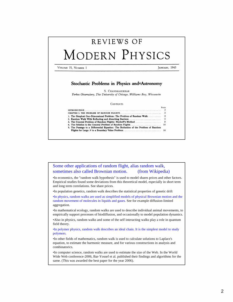
Chandrasekhar has contributed significantly to the theory of random flight (see next page), and it is therefore surprising that he did not consider to use this concept for radiative transfer. The reason may be his lack of computing power, which is needed to make practical use of the random flight concept. Without a computer, the only way to solve radiative transfer problems was to set up equations, and try to solve them analytically for the given boundary conditions. But this is only possible for most simple geometries...

However, an urgent practical need for solving the transfer problems in arbitrary geometriesarised in the 50s, with the development of nuclear power. Photons were replaced by neutrons, but the problems were the same. At that time, the practical tool for solving random flight problems began to emerge, namely

Monte Carlo simulation...

2

Some other applications of random flight, alias random walk, sometimes also called Brownian motion. (from Wikipedia)•In economics, the "random walk hypothesis" is used to model shares prices and other factors. Empirical studies found some deviations from this theoretical model, especially in short term and long term correlations. See share prices.

•In population genetics, random walk describes the statistical properties of genetic drift

•In physics, random walks are used as simplified models of physical Brownian motion and the random movement of molecules in liquids and gases.See for example diffusion-limited aggregation.

•In mathematical ecology, random walks are used to describe individual animal movements, to empirically support processes of biodiffusion, and occasionally to model population dynamics.

•Also in physics, random walks and some of the self interacting walks play a role in quantum field theory.

•In polymer physics, random walk describes an ideal chain. It is the simplest model to study polymers.

•In other fields of mathematics, random walk is used to calculate solutions to Laplace'sequation, to estimate the harmonic measure, and for various constructions in analysis and combinatorics.

•In computer science, random walks are used to estimate the size of the Web. In the World Wide Web conference-2006, Bar-Yossef et al. published their findings and algorithms for the same. (This was awarded the best paper for the year 2006).

3

•In brain research, random walks and reinforced random walks are used to model cascades of neuron firing in the brain.

•In vision science, fixational eye movements are well described by a random walk.

•In psychology,random walks explain accurately the relation between the time needed to make a decision and the probability that a certain decision will be made. (Nosofsky, 1997)

•Random walk can be used to sample from a state space which is unknown or very large, for example to pick a random page off the internet or, for research of working conditions, a random illegal worker in a given country.

•When this last approach is used in computer science it is known as Markov Chain Monte Carlo or MCMC for short. Often, sampling from some complicated state space also allows one to get a probabilistic estimate of the space's size. The estimate of the permanent of a large matrix of zeros and ones was the first major problem tackled using this approach.

•In wireless networking, random walk is used to model node movement.

•Bacteria engage in a biased random walk.

•Random walk is used to model gambling.

•In physics, random walks underlying the method of Fermi estimation.

•During World War II a random walk was used to model the distance that an escaped prisoner of war would travel in a given time.

Wikipedia page on random walk is not particularly good...

Implicit assumptions of classical radiative transfer:1. Energy of electromagnetic radiation is carried by particles

called photons. A photon carries an energy quantum2ω πν=

2. In vacuum, photons travel on straight lines,in direction , with constant speed c.Each photon carries a momentum quantum

ˆ ˆok

c

ω= = =p k s sℏ ℏ ℏ

s

2 2ˆ ,νs1 1

ˆ ,νs3 3ˆ ,νs

4 4ˆ ,νs

3. Photons interact with atoms and molecules of the matter,exchanging thereby energyand momentum. Momentum exchange is accompanied by a change of the flight directions

E hω ν= =ℏ

/E c=p

4

θ

pi i, E ki

ks q

ps s, E

∆ ∆ p, E

We shall only consider two extreme types of exchange processes:

1. Quasi-elastic scattering:

p , E ∆ ∆ p p = , E = Ei i ii

2. Absorption (extremely inelastic scattering):

/ / 0i iE E ω ω∆ = ∆ ≈

i s≈k k

Photon re-emerges with almost the same energy,but changes flight direction:

Matter takes all energy and momentum of the photon:

Keep, however, in mind that the energy stored in matter can be laterre-emitted as, e.g., thermal radiation!!!

scatteringvector

/= ∆q p ℏ

1. Energy of electromagnetic radiation is carried by particles called photons. A photon carries an energy quantum

E hω ν= =ℏ

2. Photons fly in a quasi-homogeneous medium, along rays of geometrical optics, with a speedcm=c/n. (n is the real part of refr. index)

Note: a photon‘s flight along a ray involves many microscopic interactions.Warning: the issue of photon speed in matter is still subject to discussions.

3. Occasionally, photons interact with inhomogeneitiesof the matter, exchanging thereby energy and momentum.

The above assumptions are sufficient to do radiative transferin interstellar space. In condensed matter there are modifications:

Here we shall neglect curved rays, but see next page.

?

5

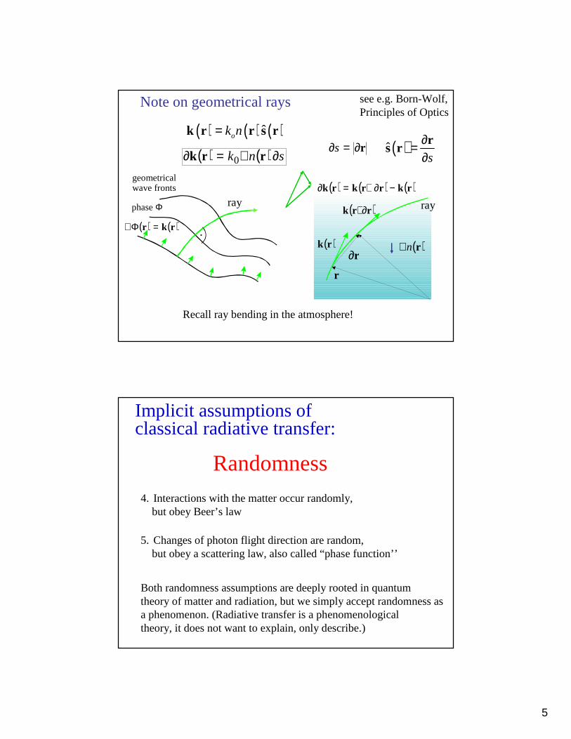
Note on geometrical rays

( ) ( ) snk ∂∇=∂ rrk 0

( ) ( )rkr =Φ∇

geometrical wave fronts

ray ray

( )rk

( )rrk ∂+

( ) ( ) ( )rkrrkrk −∂+=∂

r∂

r

r∂=∂s

( )rn∇

( ) ( ) ( )ˆok n=k r r s r

( )ˆs

∂=∂r

s r

Recall ray bending in the atmosphere!

see e.g. Born-Wolf, Principles of Optics

phaseΦ

Implicit assumptions of classical radiative transfer:

4. Interactions with the matter occur randomly,but obey Beer’s law

5. Changes of photon flight direction are random,but obey a scattering law, also called “phase function’’

Randomness

Both randomness assumptions are deeply rooted in quantum theory of matter and radiation, but we simply accept randomness asa phenomenon. (Radiative transfer is a phenomenologicaltheory, it does not want to explain, only describe.)

6

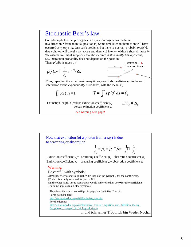
Stochastic Beer’s law Consider a photon that propagates in a quasi-homogeneous mediumin a direction from an initial position r o. Some time later an interaction will have occurred at . One can’t predict s, but there is a certain probability p(s)δsthat a photon will travel a distance s and then will interact within a short distance δs.We assume for initial simplicity that the medium is statistically homogeneous,i.e., interaction probability does not depend on the position. Then p(s)δs is given by

/1( ) e e

e

sp s s sδ δ−= ℓ

ℓ

s

Thus, repeating the experiment many times, one finds the distance s to the next interaction event exponentially distributed, with the mean

0( ) es s p s ds

∞= =∫ ℓ

eℓ

ˆi o s= +r r s

0( ) 1p s ds

∞=∫

1/ e eµ=ℓExtinction length versus extinction coefficient µe

versus extinction coefficient γe

see warning next page!

eℓ

sscatteringor absorption

*

**

*

Warning:Be careful with symbols! Atmosphere scholars would rather die than use the symbol µµµµ for the coefficients. (Their µ is strictly reserved for µ=cosθ). On the other hand, tissue researchers would rather die than use γγγγ for the coefficients.The same applies to all other symbols!!

Therefore, there are two Wikipedia pages on Radiative Transfer:For the atmosphere:http://en.wikipedia.org/wiki/Radiative_transferFor the tissues: http://en.wikipedia.org/wiki/Radiative_transfer_equation_and_diffusion_theory_for_photon_transport_in_biological_tissue

... und ich, armer Tropf, ich bin Weder Noch...

1 1 1e s a

e s a

µ µ µ= = + = +ℓ ℓ ℓ

Extinction coefficient µe= scattering coefficient µs + absorption coefficient µa

Extinction coefficient γe= scattering coefficient γs+ absorption coefficient γa

Note that extinction (of a photon from a ray) is due to scattering or absorption

7

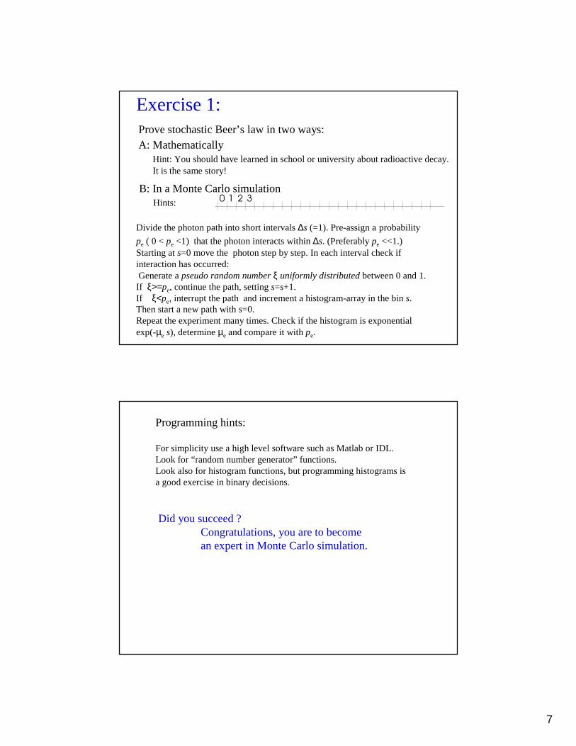
Exercise 1: Prove stochastic Beer’s law in two ways:A: Mathematically

Hint: You should have learned in school or university about radioactive decay.It is the same story!

B: In a Monte Carlo simulationHints: 0 1 2 3

Divide the photon path into short intervals ∆s (=1). Pre-assign a probability

pe ( 0 < pe <1) that the photon interacts within ∆s. (Preferably pe <<1.)Starting at s=0 move the photon step by step. In each interval check if interaction has occurred: Generate a pseudo random numberξ uniformly distributedbetween 0 and 1.If ξ>=pe, continue the path, setting s=s+1. If ξ<pe, interrupt the path and increment a histogram-array in the bin s. Then start a new path with s=0.Repeat the experiment many times. Check if the histogram is exponentialexp(-µe s), determine µe and compare it with pe.

Programming hints:

For simplicity use a high level software such as Matlab or IDL.Look for “random number generator” functions.Look also for histogram functions, but programming histograms isa good exercise in binary decisions.

Did you succeed ?Congratulations, you are to become an expert in Monte Carlo simulation.

8

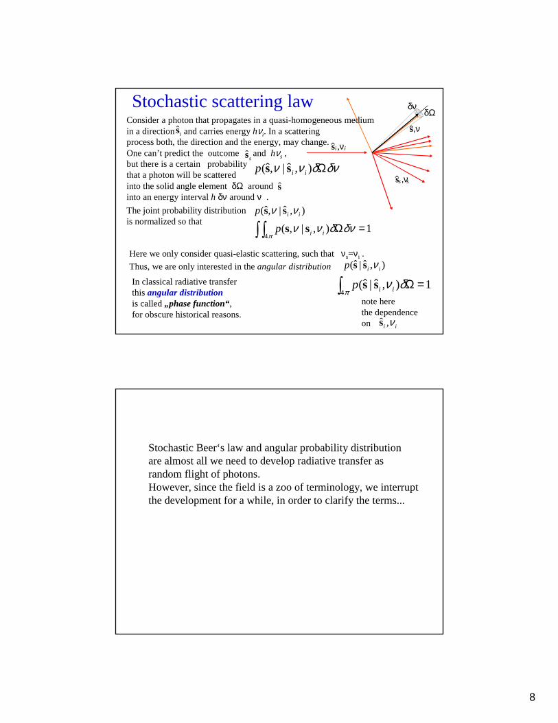
Consider a photon that propagates in a quasi-homogeneous mediumin a direction and carries energy hνi. In a scattering process both, the direction and the energy, may change. One can’t predict the outcome and hνs , but there is a certain probabilitythat a photon will be scatteredinto the solid angle element δΩ around into an energy interval h δν around ν .

Stochastic scattering law

4ˆ ˆ( | , ) 1i ip

πν δΩ =∫ s s

ˆ ˆ( , | , )i ip ν ν δ δνΩs s

4( , | , ) 1i ip

πν ν δ δνΩ =∫ ∫ s s

ˆis

ˆss

s ,ν

s ,ν

s,ν

^

^

^

δΩδν

s

i i

ss

The joint probability distribution is normalized so that

ˆ ˆ( , | , )i ip ν νs s

Here we only consider quasi-elastic scattering, such that νs=νi .

Thus, we are only interested in the angular distribution ˆ ˆ( | , )i ip νs s

In classical radiative transfer this angular distributionis called „phase function“, for obscure historical reasons.

note herethe dependenceon ˆ ,i iνs

Stochastic Beer‘s law and angular probability distributionare almost all we need to develop radiative transfer asrandom flight of photons. However, since the field is a zoo of terminology, we interruptthe development for a while, in order to clarify the terms...

9

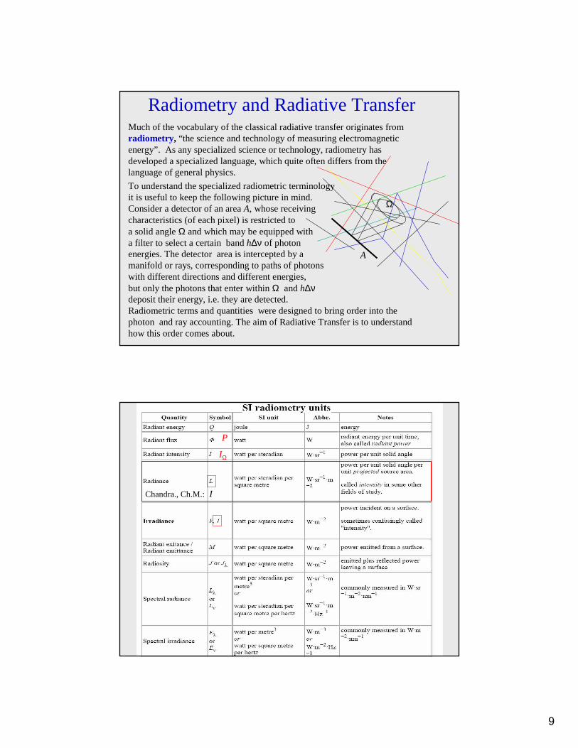
To understand the specialized radiometric terminologyit is useful to keep the following picture in mind.Consider a detector of an area A, whose receiving characteristics (of each pixel) is restricted to a solid angle Ω and which may be equipped with a filter to select a certain band h∆ν of photon energies. The detector area is intercepted by a manifold or rays, corresponding to paths of photons with different directions and different energies, but only the photons that enter within Ω and h∆νdeposit their energy, i.e. they are detected. Radiometric terms and quantities were designed to bring order into the photon and ray accounting. The aim of Radiative Transfer is to understandhow this order comes about.

Radiometry and Radiative TransferMuch of the vocabulary of the classical radiative transfer originates from radiometry , “the science and technology of measuring electromagnetic energy”. As any specialized science or technology, radiometry has developed a specialized language, which quite often differs from the language of general physics.

A

Ω

IΩ

Chandra., Ch.M.:I

P

10

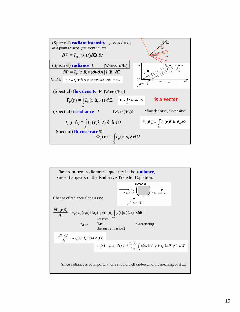
(Spectral)radiant intensity IΩ [W/sr (/Hz)]of a point source (far from source)

ˆ( , )P I νδ ν δ δνΩ= Ωs

(Spectral)radiance L [W/m2/sr (/Hz)]

ˆ ˆ ˆ( , , ) | |P L Aνδ ν δνδ δ= ⋅ Ωr s s n n s

(Spectral)flux density F [W/m2 (/Hz)]

ˆ ˆ( ) ( , , )L dν ν νΩ

= Ω∫F r r s s

ˆ ˆ ˆ ˆ( ; ) ( , , )I L dν ν νΩ

= ⋅ Ω∫r n r s s n

(Spectral)irradiance I [W/m2(/Hz)]

is a vector!

(Spectral)fluence rate Φˆ( ) ( , , )L dν ν ν

Ω

Φ = Ω∫r r s

“flux density”, “intensity”

Ch.M:

The prominent radiometric quantity is the radiance, since it appears in the Radiative Transfer Equation:

4

ˆ( , )ˆ ˆ ˆ ˆ ˆ( , ) ( , ) ( | ) ( , )e s

LL S p L d

sν

ν ν νπ

µ µ∂ ′ ′ ′= − + + Ω∂ ∫

r sr s r s s s r s

Beer

sources(laser, thermal emission)

in-scattering

Change of radiance along a ray:

Since radiance is so important, one should well understand the meaning of it ....

11

Radianceby S.L. Jacques, S. A. Prahl Oregon Graduate Institute

Source Target

A->0

Ω->0

ˆ,ˆ ˆ ˆ( , )P L Aδ δ δ= ⋅ Ωr s r s n s

ˆ ˆ ˆ( )A s

A

P dA I A= ⋅ = ⋅∫F n s n

n

ˆ ˆ ˆ( ) sL d IΩ

= Ω =∫F s s s

I

I

Consider for example a surface illuminated by sun

ˆ ˆ ˆ( ) ( )sL Iδ= −s s s

ˆssIrradiance I

Radiance

Power

The term radiance does not explicitly occur in the random flight. But radiance is realized through an ensemble of random flights.

However, we shall need the irradiance:

12

From photon stochastics to radiometry

Before proceeding to random flight, we try to connect some of theradiometry concepts with general physics...

Simple model: scattering on a single particle

r

δaδΩ δ = a/r

2

θ

σA

Consider a beam of photons that come flying in the direction s, randomly but uniformly distributed over a cross-section area A.

Meanpower carried by the beam isP [W],or Pphot=P/hν [photons/s].

These photons interact with a target of a scattering cross-sectionσS. (σS is not the geometrical cross-section of the target!)

Theprobability that a photon „hits the target“ is ps= σS/A.Thus, the totalmeanscattered power is

/s s S SP p P P A Iσ σ= = =

Irradiance: I = P/A

S

13

r

δaδΩ δ = a/r

2

θ

σA

The scattered photons are distributed according to theangular distribution

Thus, themeanpower scattered in a solid angle elementδΩarounds is:

The quantityIΩ is theradiant intensity [W/sr]

ˆ ˆ ˆ ˆ( | , ) ( | , )i i i i SI p Iν δ ν δ σΩ Ω = Ωs s s s

ˆ ˆ( | , )i ip νs s

Note: Many people would callI and IΩ „intensity“. But intensity is themost abused word in physics. Therefore, specialists working in radiometrydecided onirradianceI (also denoted withE) andradiant intensityIΩ.

steradian sr

S

ˆ ˆ( | , )ˆ ˆ ˆ ˆ( | , ) ( | , )i i

i i i i S

Ip

I

νσ ν ν σΩ∂ = =s ss s s s

Physicist’s point of view:

Differential scattering cross-section:

4S πσ δσ = ∂ Ω∫Total scattering cross-section:

Physicist defines the „phase function“ as ˆ ˆ( | , )

ˆ ˆ( | , )ˆ ˆ( | , )

i ii i

S i i

pσ νν

νσ∂≡ s s

s ss s

Notes:

People working in microwave remote sensing prefer radar terminology, such as bistatic cross-section, which seems to differ from the physicistsdifferential cross-section by a factor 4π (ask Christian).

ˆ ˆ( | , )i i

δσ σ νδ

≡ ∂Ω

s sA frequent but rather strange notation for ∂σ is

14

Thus, upon crossing the scattering layer, the power carried by the beamhas changed by a small amount

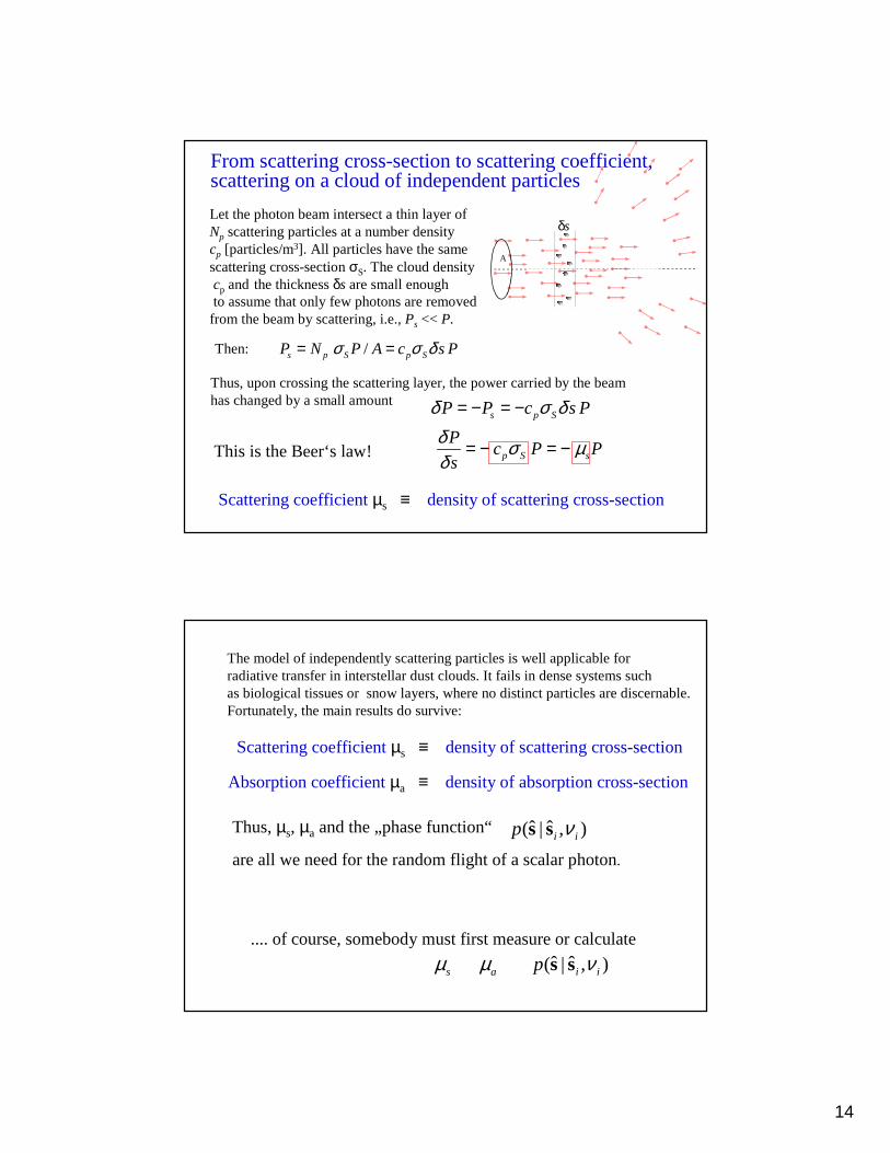
From scattering cross-section to scattering coefficient, scattering on a cloud of independent particles

A

δsLet the photon beam intersect a thin layer ofNp scattering particles at a number densitycp [particles/m3]. All particles have the same scattering cross-section σS. The cloud densitycp and the thickness δs are small enoughto assume that only few photons are removedfrom the beam by scattering, i.e., Ps << P.

Then: /s p S p SP N P A c s Pσ σ δ= =

s p SP P c s Pδ σ δ= − = −

This is the Beer‘s law! p S s

Pc P P

s

δ σ µδ

= − = −

Scattering coefficientµs ≡ density of scattering cross-section

The model of independently scattering particles is well applicable for radiative transfer in interstellar dust clouds. It fails in dense systems such as biological tissues or snow layers, where no distinct particles are discernable. Fortunately, the main results do survive:

Scattering coefficientµs ≡ density of scattering cross-section

Absorption coefficientµa ≡ density of absorption cross-section

Thus, µs, µa and the „phase function“

are all we need for the random flight of a scalar photon.

ˆ ˆ( | , )i ip νs s.... of course, somebody must first measure or calculate

aµsµ

ˆ ˆ( | , )i ip νs s

15

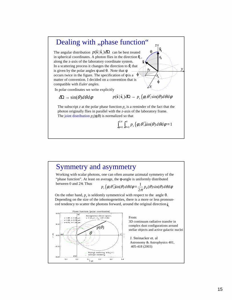
The angular distribution can be best treatedin spherical coordinates. A photon flies in the direction si ,along the z-axis of the laboratory coordinate system.In a scattering process it changes the direction to s, thatis given by the polar angles φ and θ. Note thatφ occurs twice in the figure. The specification of φ is amatter of convention. I decided on a convention that iscompatible with Euler angles.

Dealing with „phase function“θˆ ˆ( | )ip δΩs s

sin( )d dδ θ θ φΩ→ ( )ˆ ˆ( | ) , sin( )i zp p d dδ φ θ θ θ φΩ→s s

In polar coordinates we write explicitly

The subscript z at the polar phase function pz is a reminder of the fact that thephoton originally flies in parallel with the z-axis of the laboratory frame. Thejoint distributionpz(φ,θ) is normalized so that

( )2

0 0, sin( ) 1zp d d

π π

φ θφ θ θ θ φ

= ==∫ ∫

^

^

Symmetry and asymmetry

( ) 1, sin( ) ( )sin( )

2zp d d p d dθφ θ θ θ φ θ θ θ φπ

=

Working with scalar photons, one can often assume azimutal symmetry of the“phase function”. At least on average, the φ-angle is uniformly distributedbetween 0 and 2π. Thus

On the other hand, pz is seldomly symmetrical with respect to the angle θ. Depending on the size of the inhomogeneities, there is a more or less pronoun-ced tendency to scatter the photons forward, around the original direction ˆ is

( )p θθ

From:3D continuum radiative transfer in complex dust configurations around stellar objects and active galactic nuclei

J. Steinacker et. alAstronomy & Astrophysics 401,405-418 (2003)

16

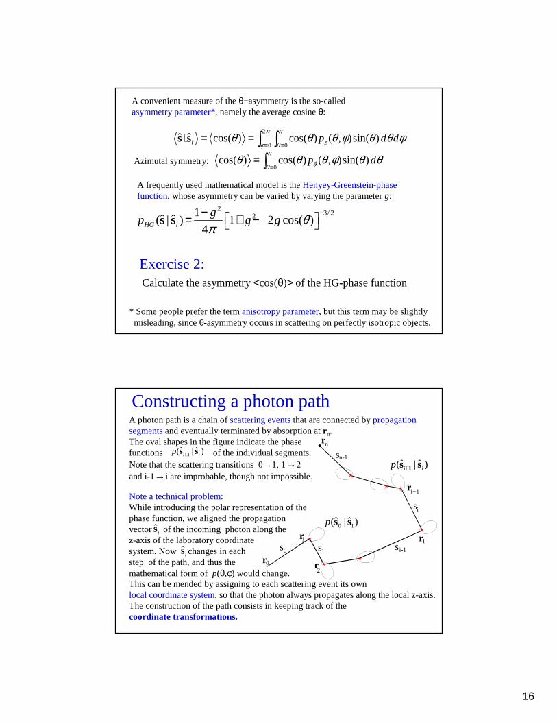
A convenient measure of the θ−asymmetry is the so-called asymmetry parameter*, namely the average cosine θ:

2

0 0ˆ ˆ cos( ) cos( ) ( , )sin( )i zp d d

π π

φ θθ θ θ φ θ θ φ

= =⋅ = = ∫ ∫s s

* Some people prefer the term anisotropy parameter, but this term may be slightlymisleading, since θ-asymmetry occurs in scattering on perfectly isotropic objects.

A frequently used mathematical model is the Henyey-Greenstein-phase function, whose asymmetry can be varied by varying the parameter g:

23/ 221

ˆ ˆ( | ) 1 2 cos( )4HG i

gp g g θ

π−−

= + − s s

Exercise 2:Calculate the asymmetry <cos(θ)> of the HG-phase function

0cos( ) cos( ) ( , )sin( )p d

π

θθθ θ θ φ θ θ

== ∫Azimutal symmetry:

rs s s

s

s

1

0

0

2

1

n-1

ii-1

i+1

i

n

r

r

r

r

r

Note a technical problem:While introducing the polar representation of the phase function, we aligned the propagationvector of the incoming photon along thez-axis of the laboratory coordinate system. Now changes in each step of the path, and thus the mathematical form of p(θ,φ) would change. This can be mended by assigning to each scattering event its ownlocal coordinate system, so that the photon always propagates along the local z-axis.The construction of the path consists in keeping track of the coordinate transformations.

Constructing a photon pathA photon path is a chain of scattering eventsthat are connected by propagation segmentsand eventually terminated by absorption at r n.The oval shapes in the figure indicate the phasefunctions of the individual segments.Note that the scattering transitions 0→1, 1→2 and i-1→i are improbable, though not impossible.

1ˆ ˆ( | )i ip +s s

1ˆ ˆ( | )i ip +s s

ˆis

ˆis

0 1ˆ ˆ( | )p s s

17

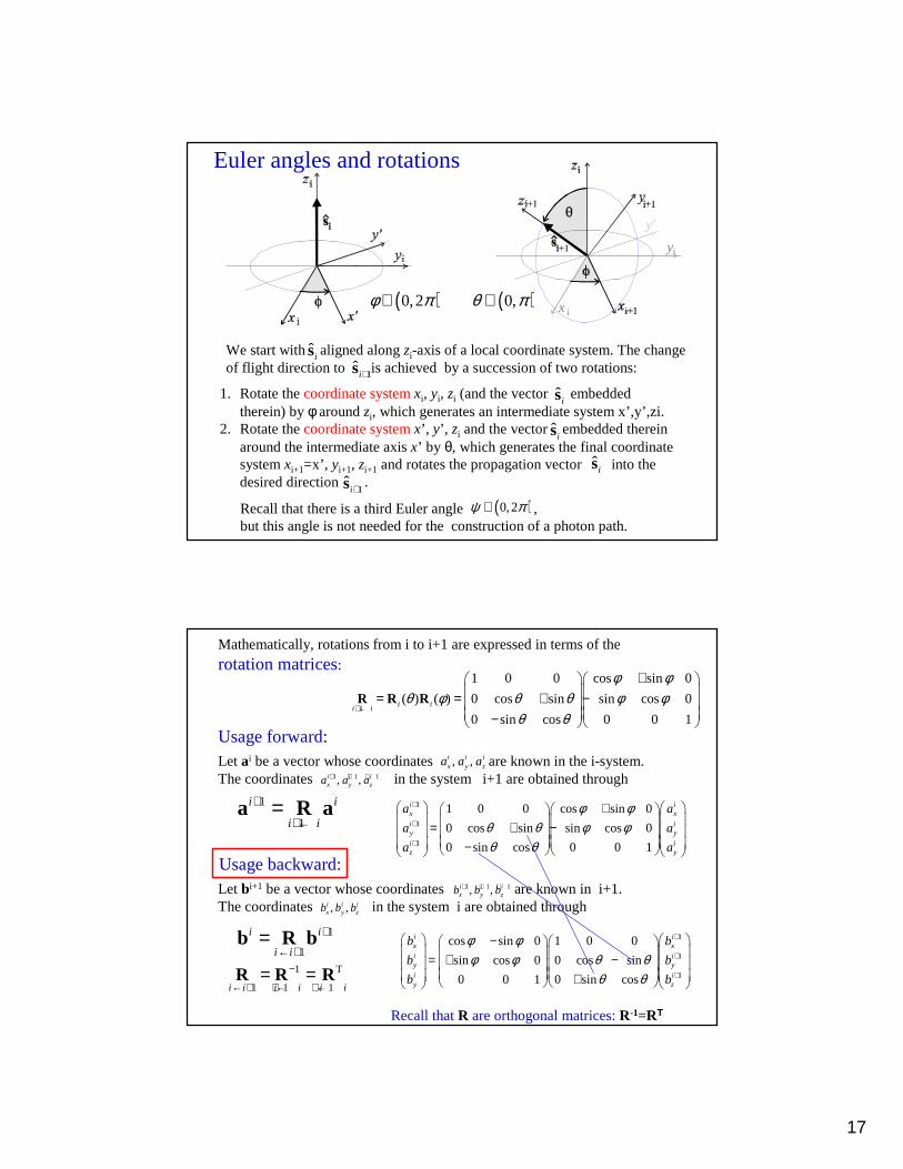
Euler angles and rotations

x

y

y'

i

i

We start with aligned along zi-axis of a local coordinate system. The changeof flight direction to is achieved by a succession of two rotations:

1. Rotate the coordinate systemxi, yi, zi (and the vector embedded therein) by φ around zi, which generates an intermediate system x’,y’,zi.

2. Rotate the coordinate systemx’, y’, zi and the vector embedded therein around the intermediate axis x’ by θ, which generates the final coordinate system xi+1=x’, yi+1, zi+1 and rotates the propagation vector into the desired direction .

ˆis

1ˆ

i+s

ˆis

ˆis

ˆis

1ˆ

i+s

Recall that there is a third Euler angle , but this angle is not needed for the construction of a photon path.

( )0,2φ π∈ ( )0,θ π∈

( )0,2ψ π∈

1

1 0 0 cos sin 0

( ) ( ) 0 cos sin sin cos 0

0 sin cos 0 0 1i i

i i

φ φθ φ θ θ φ φ

θ θ+ ←

+ = = + − −

R R R

Mathematically, rotations from i to i+1 are expressed in terms of the

rotation matrices:

Usage forward:Let ai be a vector whose coordinates are known in the i-system.The coordinates in the system i+1 are obtained through

, ,i i ix y za a a

1 1 1, ,i i ix y za a a+ + +

1

1

i i

i i

+

+ ←=a R a 1

1

1

1 0 0 cos sin 0

0 cos sin sin cos 0

0 sin cos 0 0 1

i ix x

i iy y

i iz y

a a

a a

a a

φ φθ θ φ φθ θ

+

+

+

+ = + −

−

Let bi+1 be a vector whose coordinates are known in i+1.The coordinates in the system i are obtained through

1

1

i i

i i

+

← +=b R b

1 T

1 1 1i i i i i i

−

← + + ← + ←= =R R R

1 1 1, ,i i ix y zb b b+ + +

, ,i i ix y zb b b

1

1

1

cos sin 0 1 0 0

sin cos 0 0 cos sin

0 0 1 0 sin cos

i ix x

i iy y

i iy z

b b

b b

b b

φ φφ φ θ θ

θ θ

+

+

+

− = + −

+

Recall that R are orthogonal matrices: R-1=RT

Usage backward:

18

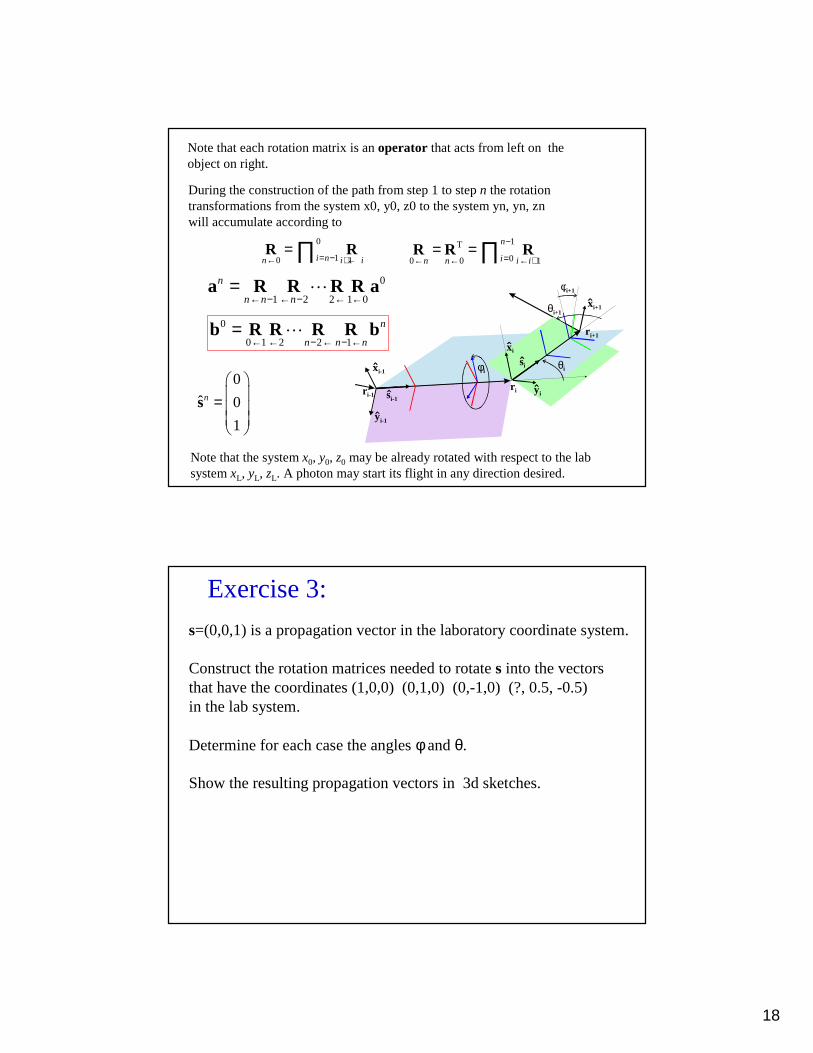
Note that the system x0, y0, z0 may be already rotated with respect to the lab system xL, yL, zL. A photon may start its flight in any direction desired.

0

10 1i nn i i= −← + ←= ∏R R

xi-1

si-1

si

yi-1

yi

xi+1

xi

r i-1r i

r i+1

φi

φi+1

θi

θi+1

During the construction of the path from step 1 to step n the rotation transformations from the system x0, y0, z0 to the system yn, yn, znwill accumulate according to

0

1 2 2 1 0

n

n n n← − ← − ← ←=a R R R R a⋯

0

ˆ 0

1

n

=

s

1T

00 0 1

n

in n i i

−

=← ← ← += = ∏R R R

Note that each rotation matrix is an operator that acts from left on theobject on right.

0

0 1 2 2 1

n

n n n← ← − ← − ←=b R R R R b⋯

Exercise 3:

s=(0,0,1) is a propagation vector in the laboratory coordinate system.

Construct the rotation matrices needed to rotate s into the vectorsthat have the coordinates (1,0,0) (0,1,0) (0,-1,0) (?, 0.5, -0.5) in the lab system.

Determine for each case the angles φ and θ.

Show the resulting propagation vectors in 3d sketches.

19

Exercise 4: Construct and plot a couple of nice pathsHints:

1. Chose the initial position r o and save it. 2. Chose initial directions0 (rotation of the coordinate system! ).3. Propagate the photon a chosen distance s0 into r 1. Save r 1.4. Chose the angles φ1 θ1 in the local system.5. Update the accumulated rotation matrix and generate s1 (in lab system).6. Propagate the photon a chosen distance s1 into r 2 (in lab system!). Save r 2

7. Goto 4 until you decide on absorption.8. Plot the path 3d

Exercise 5: Use your program to construct and plot this 3d path:

0

1

2

3

4

5

6 7 89

10

x

z

y

Use Matlab, or Maple, or IDL, or Mathematica, or ....

Application examples from Wikipedia

Graphics, particularly for ray tracing; a version of the Metropolis-Hastings algorithm is alsoused for ray tracing where it is known as Metropolis light transport

Modeling light transport in biological tissueMonte Carlo methods in financeReliability engineeringIn simulated annealing for protein structure predictionIn semiconductor device research, to model the transport of current carriersEnvironmental science, dealing with contaminant behaviorSearch And Rescue and Counter-Pollution. Models used to predict the drift of a life raft or movement of an oil slick at sea.

In probabilistic design for simulating and understanding the effects of variabilityIn physical chemistry, particularly for simulations involving atomic clustersIn polymer physics: Bond fluctuation modelIn computer science: Las Vegas algorith, LURCH, Computer go General Game Playing

Monte Carlo basics

not only for random flight!

20

Modeling the movement of impurity atoms (or ions) in plasmas in existing and tokamaks(e.g.: DIVIMP).

Nuclear and particle physics codes using the Monte Carlo method:GEANT — CERN's simulation of high energy particles interacting with a detector.CompHEP, PYTHIA — Monte-Carlo generators of particle collisionsMCNP(X) - LANL's radiation transport codesMCU: universal computer code for simulation of particle transport (neutrons, photons,electrons) in three-dimensional systems by means of the Monte Carlo methodEGS — Stanford's simulation code for coupled transport of electrons and photonsPEREGRINE: LLNL's Monte Carlo tool for radiation therapy dose calculationsBEAMnrc — Monte Carlo code system for modeling radiotherapy sources (LINAC's)PENELOPE — Monte Carlo for coupled transport of photons and electrons, with applications in radiotherapyMONK — Serco Assurance's code for the calculation of k-effective of nuclear systems

Modelling of foam and cellular structuresModeling of tissue morphogenesisComputation of holograms Phylogenetic analysis, i.e. Bayesian inference, Markov chain Monte Carlo

Implicit assumptions of classical radiative transfer:

4. Interactions with the matter occur randomly,but obey Beer’s law

5. Changes of photon flight direction are random,but obey a scattering law, also called “phase function’’

Randomness

Both assumptions are deeply rooted in quantum theory ofmatter and radiation, but we simply accept randomness asa phenomenon. (Radiative transfer is a phenomenologicaltheory, it does not want to explain, only describe.)

21

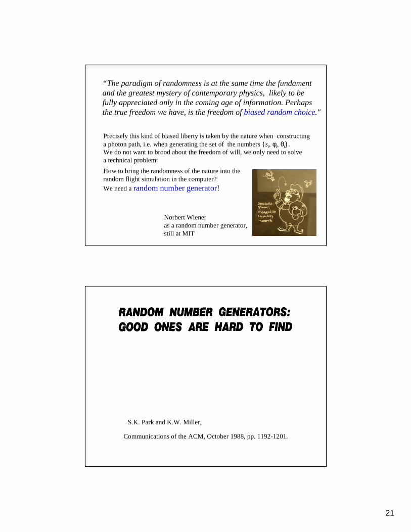
“The paradigm of randomness is at the same time the fundament and the greatest mystery of contemporary physics, likely to be fully appreciated only in the coming age of information. Perhapsthe true freedom we have, is the freedom of biased random choice."

Precisely this kind of biased liberty is taken by the nature when constructing a photon path, i.e. when generating the set of the numbers si, φi, θi.We do not want to brood about the freedom of will, we only need to solve a technical problem:

How to bring the randomness of the nature into the random flight simulation in the computer?

We need a random number generator!

Norbert Wieneras a random number generator,still at MIT

S.K. Park and K.W. Miller,

Communications of the ACM, October 1988, pp. 1192-1201.

22

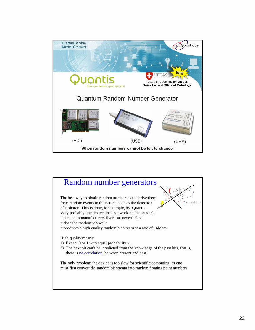
Random number generators

The best way to obtain random numbers is to derive them from random events in the nature, such as the detection of a photon. This is done, for example, by Quantis. Very probably, the device does not work on the principle indicated in manufacturers flyer, but nevertheless, it does the random job well: it produces a high quality random bit stream at a rate of 16Mb/s.

High quality means: 1) Expect 0 or 1 with equal probability ½. 2) The next bit can’t be predicted from the knowledge of the past bits, that is,

there is no correlation between present and past.

The only problem: the device is too slow for scientific computing, as one must first convert the random bit stream into random floating point numbers.

23

For our purpose, it is sufficient to use a software based generator of pseudo-random numbers (PRNG), which is a part of every package for scientific computing.

A PRNG computes, starting from a “seed”, a deterministic chain (stream) of numbers, whose frequency of occurrence fulfills the specified distribution (basically uniform), and which look random, if the seed and the algorithm are not known.

Note, that starting from the same seed, one always gets the same chain of numbers!

Note, that there is often a trade-off between speed and quality, in particular thecriterion “no correlation”is not always well fulfilled.

Pseudo-random number generators

More on random number generators:http://en.wikipedia.org/wiki/Random_number_generatorand references therein.

1. We want to choose a random number s∈0,∞ from the uni-variate distribution

2. We want to choose a pair of random numbers φ∈0,2π and θ∈0,πfrom the bi-variate distribution

Monte Carlo: Sampling a path step

( )( , ) , sin( )zp d d p d dφ θ θ φ φ θ θ θ φ=

( ) e esep s s sµδ µ δ−=

The basic version of the PRNG generates random numbers ξ that areuniformly distributedin the interval 0,1. We must learn how to transform ξ into the random number from the desired distributions, namely from theBeer’s law and from the phase function. More precisely

23 / 221

( , ) 1 2 cos( ) sin( )4

gp d d g g d dφ θ θ φ θ θ θ φ

π−−

= + − Henyey-Greenstein:

Uniform over sphere:1

( , ) sin( )4

p d d d dφ θ θ φ θ θ φπ

=

To be specific, e.g.:

24

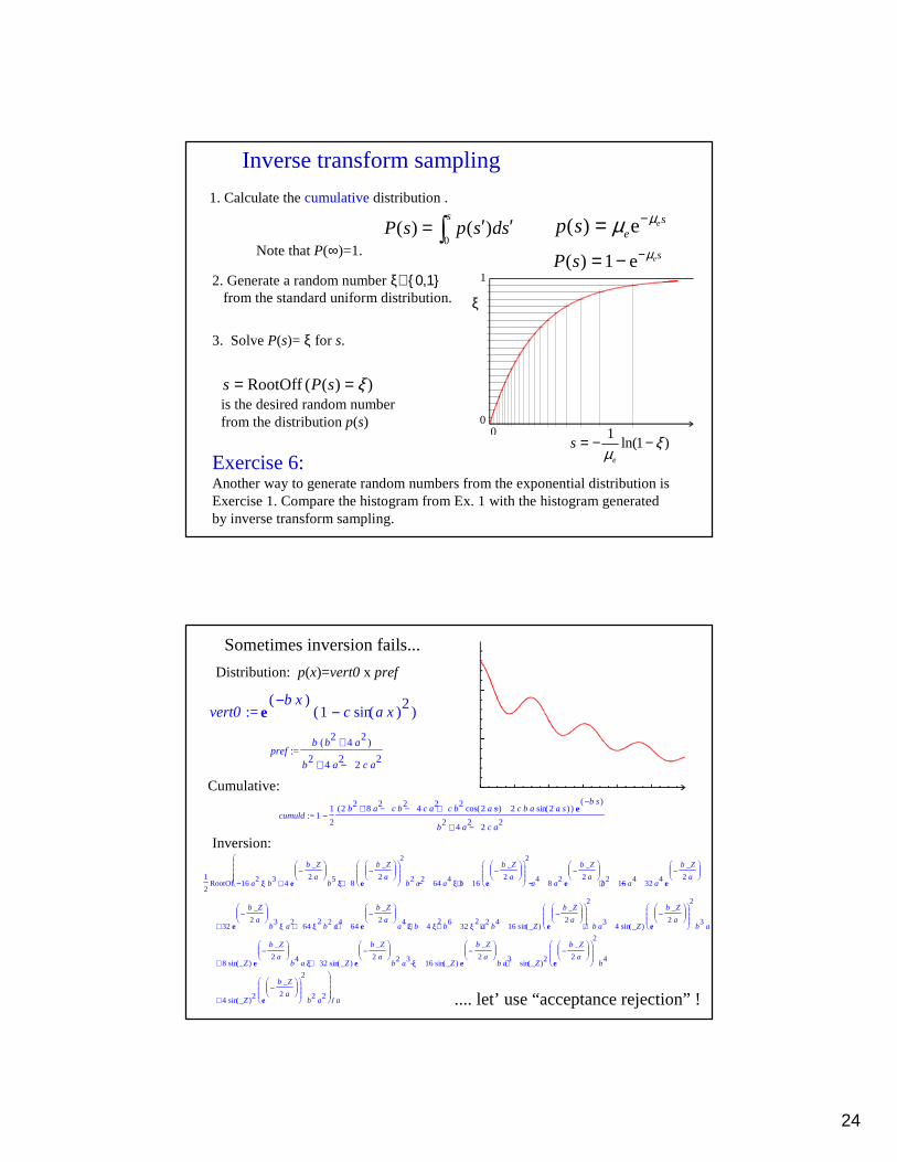
Exercise 6:Another way to generate random numbers from the exponential distribution isExercise 1. Compare the histogram from Ex. 1 with the histogram generatedby inverse transform sampling.

2. Generate a random number ξ∈0,1from the standard uniform distribution.

Inverse transform sampling

1. Calculate the cumulative distribution .

0( ) ( )

sP s p s ds′ ′= ∫ ( ) e es

ep s µµ −=

( ) 1 e esP s µ−= −

is the desired random number from the distribution p(s)

1ln(1 )

e

s ξµ

= − −

3. Solve P(s)= ξ for s.

RootOff ( ( ) )s P s ξ= =

00

1

ξ

Note that P(∞)=1.

1

2RootOf 16a

2 ξ b3 4 e

−

b _Z

2 ab

5 ξ 8

e

−

b _Z

2 a

2

b2

a2 64a

4 ξ b 16

e

−

b _Z

2 a

2

a4 8 a

2e

−

b _Z

2 ab

2 16a4 32a

4e

−

b _Z

2 a− + + − + − + −

32e

−

b _Z

2 ab

3 ξ a2

64ξ2

b2

a4

64e

−

b _Z

2 aa

4 ξ b 4 ξ2

b6

32ξ2

a2

b4

16 ( )sin _Z

e

−

b _Z

2 a

2

b a3

4 ( )sin _Z

e

−

b _Z

2 a

2

b3

a + + + + + + +

8 ( )sin _Z e

−

b _Z

2 ab

4a ξ 32 ( )sin _Z e

−

b _Z

2 ab

2a

3 ξ 16 ( )sin _Z e

−

b _Z

2 ab a

3 ( )sin _Z2

e

−

b _Z

2 a

2

b4 + + − +

4 ( )sin _Z2

e

−

b _Z

2 a

2

b2

a2 +

a /

:= vert0 e( )−b x

( ) − 1 c ( )sin a x2

:= prefb ( ) + b

24 a

2

+ − b2

4 a2

2 c a2

Cumulative:

Inversion:

:= cumuld − 11

2

( ) + − − + − 2 b2

8 a2

c b2

4 c a2

c b2

( )cos 2a s 2 c b a ( )sin 2a s e( )−b s

+ − b2

4 a2

2 c a2

Sometimes inversion fails...

.... let’ use “acceptance rejection” !

Distribution: p(x)=vert0x pref

25

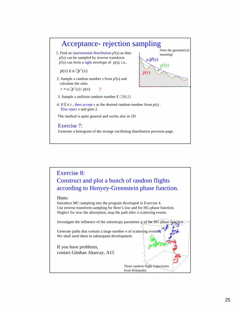
Acceptance- rejection sampling1. Find an instrumental distributionpI(s) so that:

pI(s) can be sampled by inverse transformpI(s) can form a tight envelope of p(s), i.e.,

( ) ( )Ip s u p s≤ ⋅pI(s)

p(s)

u⋅pI(s)

2. Sample a random number s from pI(s) andcalculate the ratio

4. If ξ ≤ r , then accepts as the desired random number from p(s) . Else rejects and goto 2.

( ) / ( )Ir u p s p s= ⋅

Note the geometricalmeaning!

The method is quite general and works also in 2D

Exercise 7:Generate a histogram of the strange oscillating distribution previous page.

3. Sample a uniform random number ξ ∈0,1

?

Exercise 8: Construct and plot a bunch of random flightsaccording to Henyey-Greenstein phase function.

Hints: Introduce MC-sampling into the program developed in Exercise 4.Use inverse transform sampling for Beer’s law and for HG-phase function.Neglect for now the absorption, stop the path after n scattering events.

Investigate the influence of the anisotropy parameter g of the HG phase function

Generate paths that contain a large number n of scattering events!We shall need them in subsequent development.

If you have problems, contact Günhan Akarcay, A15

Three random flight trajectoriesfrom Wikipedia

26

http://cg.scs.carleton.ca/~luc/rnbookindex.html

Ilya M. Sobol –A Primer for the Monte Carlo Method (1994)

www.scribd.com/doc/8749827/Ilya-M-Sobol-A-Primer-for-the-Monte-Carlo- Method-1994

Luc DevroyeNon-Uniform Random Variate Generation

Applying the concepts of coordinate transformationsphoton paths, Monte Carlo, Radiative Transfer

27

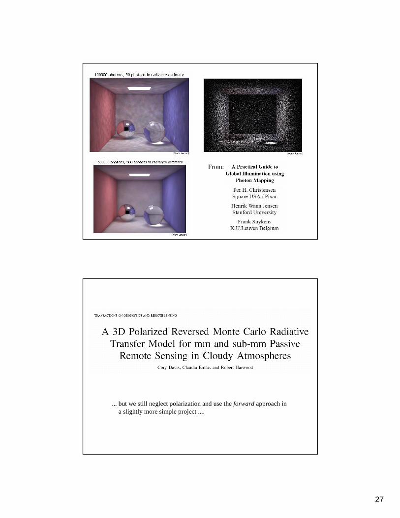
From:

... but we still neglect polarization and use the forward approach in a slightly more simple project ....

28

MC simulation project:Determine the position dependence of the rate of deposition of solar energy in a cloud... or in a sunbathers skin

This is a demanding project, worth almost a PhD. We shall only define the tasks, develop the outline of a computer program,and rehearse what we have done so far...

1. Define coordinate system....

Tasks:

Note: Planck distribution is not good for inversion sampling.One would try acceptance-rejection or search in literature.

4

/

15 1( )

e 1h kT

hb

kT ννν

υ π = − Planck’s law:

ˆ ˆ ˆ( ) ( ) ( ) | |A s

A

P dA I Aν ν ν= ⋅ = ⋅∫F n s n

ˆ ˆ ˆ( ) ( , ) ( ) sL d Iν ν νΩ

= Ω =∫F s s s

ˆ ˆ ˆ( , , ) ( ) ( )sL Iν ν δ= −r s s s

( )A AP P dν ν= ∫

2.1 Geometry: Uniformly distributed sunrays with unique direction Spectral flux density . Recall that flux density is a vector.

2. Define solar radiation

ˆ ,S S Sθ φ≡s

A

ˆ( , ) ( ) SIν ν=F r s

2.2 Spectral distribution of irradiance:

( ) ( )I Ibν ν=

29

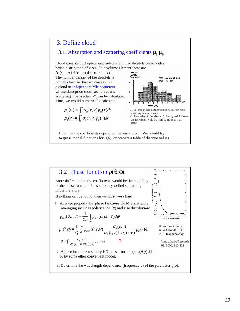
3.1. Absorption and scattering coefficientsµs µa

Cloud-droplet-size distribution from lidar multiple-scattering measurementsY. Benayahu, A. Ben-David, S. Fastig, and A.CohenApplied Optics, Vol. 34, Issue 9, pp. 1569-1578 (1995)

Cloud consists of droplets suspended in air. The droplets come with a broad distribution of sizes. In a volume element there are δn(r) = pn(r)δr droplets of radius r.The number density of the droplets is perhaps low, so that we can assume a cloud of independent Mie-scatterers,whose absorption cross-section σa andscattering cross-section σs can be calculated.Thus, we would numerically calculate

0( ) ( , ) ( )a a nr p r drµ ν σ ν

∞= ∫

0( ) ( , ) ( )s s nr p r drµ ν σ ν

∞= ∫

Note that the coefficients depend on the wavelength! We would tryto guess model functions for µ(ν), or prepare a table of discrete values.

3. Define cloud

More difficult than the coefficients would be the modeling of the phase function. So we first try to find something in the literature...

Phase functions of mixed cloudsA.A. Kokhanovsky

Atmospheric Research89, 2008, 218-221

0

( , )1( , ) ( ; , ) ( )

( , ) ( , )S

mie nS A

rp p r p r dr

Q r r

σ νθ φ θ νσ ν σ ν

∞=

+∫

3.2 Phase functionp(θ,φ).

If nothing can be found, then we must work hard:

1. Average properly the phase functions for Mie scattering. Averaging includes polarization (φ) and size distribution:

2. Approximate the result by HG-phase function pHG(θ;g(ν)) or by some other convenient model.

3. Determine the wavelength dependence (frequency ν) of the parameter g(ν).

?

0

( , )( )

( , ) ( , )S

nS A

rQ p r dr

r r

σ νσ ν σ ν

∞=

+∫ ?

2

1( ; , ) ( , ; , )

2mie miep r p r dπ

θ ν θ φ ν φπ

= ∫

30

3. 3. Define cloud: form, boundary.

This task sounds easy, but it is not... We must somehow tell the photon ata position r = (x,y,z) if it is inside the cloud or outside. This would be easy in simple geometries:

Inside:

X

Z

R

x>0 AND x<XAND y >0 AND y<YAND z>0 AND z<Z

x2+y2+z2 < R2

Exercise 10: define inside of an ellipsoid

?

However, clouds come in different shapes and clouds may be inhomogenous.To specify a general cloud, one would use meshing techniquesthat areemployed in scientific simulation software (such as COMSOL), or in 3D computer graphics („virtual reality“).

3. 3. Define cloud: form, boundary.

The simplest way to specify the cloud is to voxelize itin a rectangular mesh: 1. Enclose the cloud in a tight rectangular box. 2. Define a 3D array cloud(NX, NY ,NZ ), the number of elements in each dimension is givenby the size of the cloud divided by the desired resolution:

NX=X/∆x, NY=Y/∆y, NZ=Z/∆y. 3. Then patiently fill out the cloud:

IF x,y, z inside cloud THEN cloud[x,y,z]=1 ELSE cloud[x,y,z]=0

XY

Z

To make an inhomogeneous cloud, one would store in the array elements pointers to cloud properties µs, µa, g parameter...

Such a voxelized cloud does not have a nice boundary. This can be improved by assigning special geometry to surface voxels:

31

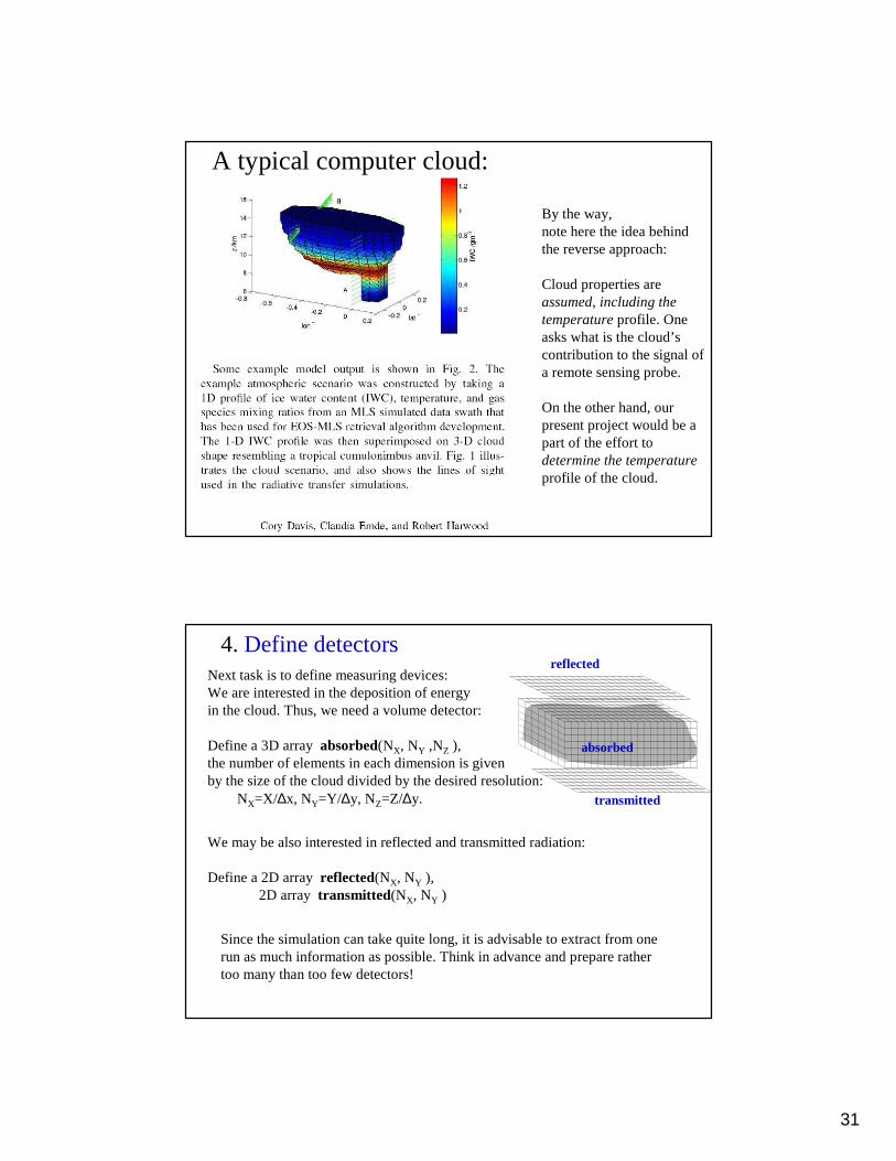
A typical computer cloud:

By the way, note here the idea behind the reverse approach:

Cloud properties are assumed, including the temperatureprofile. One asks what is the cloud’s contribution to the signal of a remote sensing probe.

On the other hand, our present project would be a part of the effort to determine the temperature profile of the cloud.

4. Define detectorsNext task is to define measuring devices: We are interested in the deposition of energyin the cloud. Thus, we need a volume detector:

Define a 3D array absorbed(NX, NY ,NZ ), the number of elements in each dimension is givenby the size of the cloud divided by the desired resolution:

NX=X/∆x, NY=Y/∆y, NZ=Z/∆y.

We may be also interested in reflected and transmitted radiation:

Define a 2D array reflected(NX, NY ), 2D array transmitted(NX, NY )

absorbed

transmitted

reflected

Since the simulation can take quite long, it is advisable to extract from onerun as much information as possible. Think in advance and prepare rathertoo many than too few detectors!

32

5. Simulation loop

5.2 Select a sun ray (uff, uff,...)

1. Define a planar surfaceS(x,y,z) that is perpendicular to the directionsS

of the sun rays.

2. Find in Sa rectangular area with sizeXp,Yp

that includes the projection of the cloud on S.

3. Sample two uniformly distributed randomnumbersξx ∈ 0,Xp and ξy ∈0,Yp.

4. Calculate fromξx ξy the intersectionxS,yS, zS of the ray with the plane S(x,y,z)

5. Trace the ray towards the cloud and determine the intersectionx0,y0,z0

with the cloud boundary. If no intersection is found, reject the ray and go to 3.

S(x,y,z)Xp,Yp

xS,yS,zS

xo,yo,zo

5.1 Select photon energy from Plank’s distribution (easy?)

5.3 Cross the cloud boundary

In general, there is reflection and refraction on a sharp boundary between two optical media. (Even a cloud can be regarded as an effective medium with an effective refractive index that is different from air.) If this is the case,then we must solve an exercise in geometry:

1. Determine the surface normal .2. Determine the “scattering plane” spanned by 3. Calculate the angle of incidence cosine4. Calculate Fresnel reflection probability R(θi).5. Sample a uniform random number x ∈0,1

IF x < R, THENphoton is reflected => [calculate reflected and continue tracingto the next boundary if desired]

ELSE photon is transmitted => calculate refracted and begin thesimulation of random flight through the cloud.....

s

ˆRs

ˆTsnn

s

n

ˆ ˆcos( )iθ = ⋅n s

s

ˆTs

33

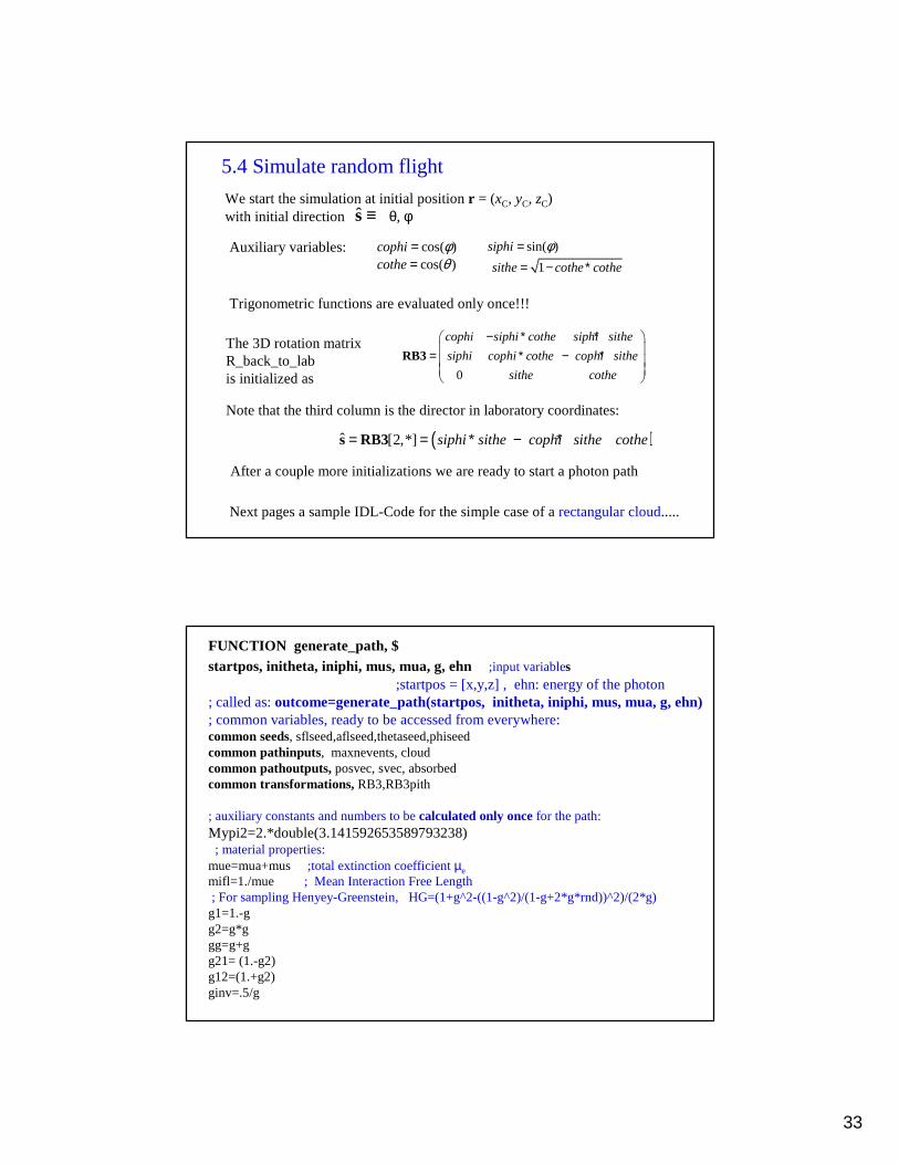
We start the simulation at initial position r = (xC, yC, zC)with initial direction θ, φ

5.4 Simulate random flight

ˆ ≡s

The 3D rotation matrixR_back_to_labis initialized as 0

cophi siphi cothe siphi sithe

siphi cophi cothe cophi sithe

sithe cothe

− ∗ ∗ = ∗ − ∗

RB3

cos( )cophi φ= sin( )siphi φ=

Note that the third column is the director in laboratory coordinates:

Auxiliary variables:

Trigonometric functions are evaluated only once!!!

1sithe cothe cothe= − ∗cos( )cothe θ=

( )ˆ [2,*] siphi sithe cophi sithe cothe= = ∗ − ∗s RB3

After a couple more initializations we are ready to start a photon path

Next pages a sample IDL-Code for the simple case of a rectangular cloud.....

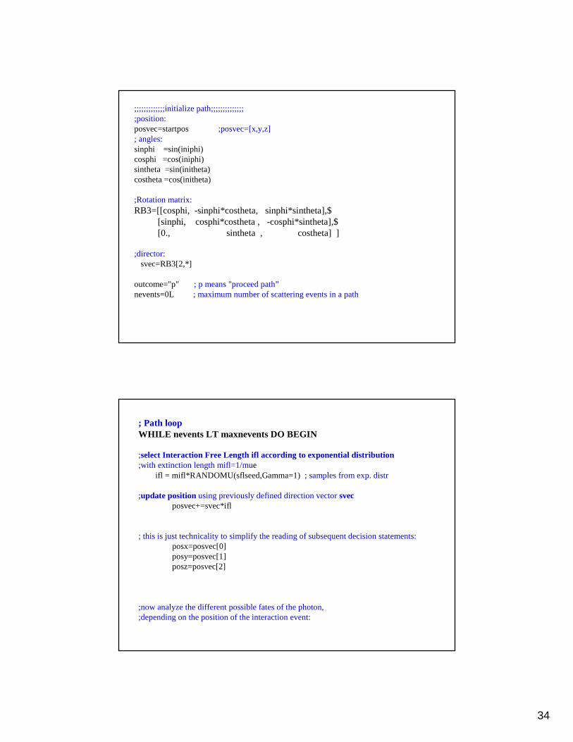
FUNCTION generate_path, $startpos, initheta, iniphi, mus, mua, g, ehn ;input variables

;startpos = [x,y,z] , ehn: energy of the photon; called as: outcome=generate_path(startpos, initheta, iniphi, mus, mua, g, ehn); common variables, ready to be accessed from everywhere:common seeds, sflseed,aflseed,thetaseed,phiseedcommon pathinputs, maxnevents, cloudcommon pathoutputs,posvec, svec, absorbedcommon transformations,RB3,RB3pith

; auxiliary constants and numbers to becalculated only oncefor the path:Mypi2=2.*double(3.141592653589793238); material properties:

mue=mua+mus ;total extinction coefficient µemifl=1./mue ; Mean Interaction Free Length; For sampling Henyey-Greenstein, HG=(1+g^2-((1-g^2)/(1-g+2*g*rnd))^2)/(2*g)g1=1.-gg2=g*ggg=g+gg21= (1.-g2)g12=(1.+g2)ginv=.5/g

34

;;;;;;;;;;;;;initialize path;;;;;;;;;;;;;;;position:posvec=startpos ;posvec=[x,y,z]; angles:sinphi =sin(iniphi)cosphi =cos(iniphi)sintheta =sin(initheta)costheta =cos(initheta)

;Rotation matrix:RB3=[[cosphi, -sinphi*costheta, sinphi*sintheta],$

[sinphi, cosphi*costheta , -cosphi*sintheta],$[0., sintheta , costheta] ]

;director:svec=RB3[2,*]

outcome="p" ; p means "proceed path”nevents=0L ; maximum number of scattering events in a path

; Path loopWHILE nevents LT maxnevents DO BEGIN

;select Interaction Free Length ifl according to exponential distribution;with extinction length mifl=1/mue

ifl = mifl*RANDOMU(sflseed,Gamma=1) ; samples from exp. distr

;update positionusing previously defined direction vector svecposvec+=svec*ifl

; this is just technicality to simplify the reading of subsequent decision statements:posx=posvec[0] posy=posvec[1]posz=posvec[2]

;now analyze the different possible fates of the photon,;depending on the position of the interaction event:

35

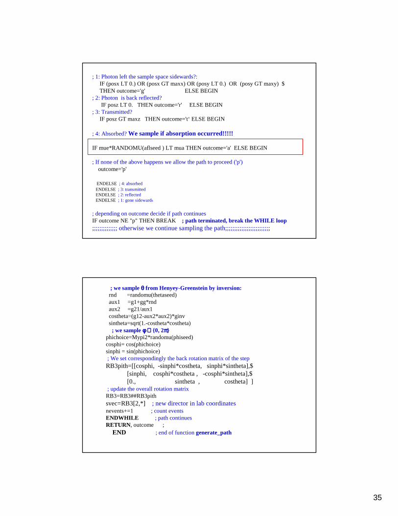
; 1: Photon left the sample space sidewards?:IF (posx LT 0.) OR (posx GT maxx) OR (posy LT 0.) OR (posy GT maxy) $THEN outcome='g' ELSE BEGIN

; 2: Photon is back reflected?IF posz LT 0. THEN outcome='r' ELSE BEGIN

; 3: Transmitted?IF posz GT maxz THEN outcome='t‘ ELSE BEGIN

; 4: Absorbed? We sample if absorption occurred!!!!!

IF mue*RANDOMU(aflseed ) LT mua THEN outcome='a' ELSE BEGIN

; If none of the above happens we allow the path to proceed ('p') outcome='p'

ENDELSE ; 4: absorbedENDELSE ; 3: transmittedENDELSE ; 2: reflectedENDELSE ; 1: gone sidewards

; depending on outcome decide if path continuesIF outcome NE "p" THEN BREAK ; path terminated, break the WHILE loop;;;;;;;;;;;;;; otherwise we continue sampling the path;;;;;;;;;;;;;;;;;;;;;;;;;

; we sample θθθθ from Henyey-Greenstein by inversion:rnd =randomu(thetaseed)aux1 =g1+gg*rndaux2 =g21/aux1costheta=(g12-aux2*aux2)*ginvsintheta=sqrt(1.-costheta*costheta); we sample φφφφ ∈∈∈∈ 0, 2ππππ

phichoice=Mypi2*randomu(phiseed)cosphi= cos(phichoice)sinphi = sin(phichoice); We set correspondingly the back rotation matrix of the step RB3pith=[[cosphi, -sinphi*costheta, sinphi*sintheta],$

[sinphi, cosphi*costheta , -cosphi*sintheta],$[0., sintheta , costheta] ]

; update the overall rotation matrixRB3=RB3##RB3pithsvec=RB3[2,*] ; new director in lab coordinatesnevents+=1 ; count eventsENDWHILE ; path continuesRETURN, outcome ;

END ; end of function generate_path

36

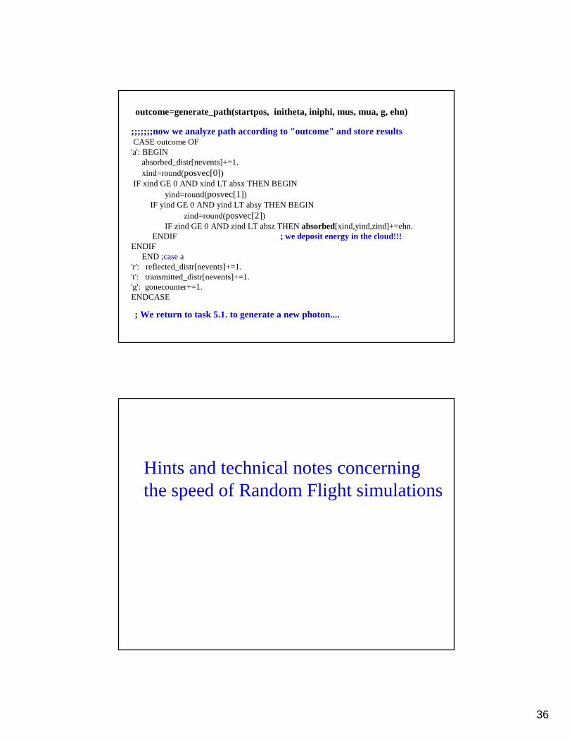
;;;;;;;now we analyze path according to "outcome" and store resultsCASE outcome OF'a': BEGIN

absorbed_distr[nevents]+=1.xind=round(posvec[0])

IF xind GE 0 AND xind LT absx THEN BEGINyind=round(posvec[1])

IF yind GE 0 AND yind LT absy THEN BEGINzind=round(posvec[2])

IF zind GE 0 AND zind LT absz THEN absorbed[xind,yind,zind]+=ehn.ENDIF ; we deposit energy in the cloud!!!

ENDIFEND ;case a

'r': reflected_distr[nevents]+=1.'t': transmitted_distr[nevents]+=1.'g': gonecounter+=1.ENDCASE

; We return to task 5.1. to generate a new photon....

outcome=generate_path(startpos, initheta, iniphi, mus, mua, g, ehn)

Hints and technical notes concerningthe speed of Random Flight simulations

37

Photons versus “photon packets”

In order to save computation time, some people suggest to propagate“photon packets” instead of individual photons. Instead of being completelyabsorbed, the packet deposits only the fraction µa/(µs+µa) of itsenergy and keeps propagating unless artificially stopped. So one hopesto achieve “variance reduction” in the same computation time.

There is in deed quite some variance reduction in the energy deposition. However, re-using of photon paths is prone to introduce statistical artifacts by amplifying improbable paths. If in doubt do not do it.

“packets”

photons

When coding a MC simulation, one should be aware of the speed of floating point operations. For example, with my notebook:

It took 6.088 seconds to perform 1000 million additions. It took 6.013 seconds to perform 1000 million multiplications. It took 15.781 seconds to perform 1000 million divisions. It took 46.648 seconds to perform 1000 million cosines. It took 31.148 seconds to perform 1000 million square roots.

It took 73.795 seconds to perform 1000 million arc-tangents. It took 32.691 seconds to perform 1000 million y.log2(x) operations.It took 55.404 seconds to perform 1000 million combined sine/cosines. It took 29.278 seconds to perform 1000 million binary exponentials.

(Benchmark software by David Harper at obliquity.com)

Speed of floating point operations

38

Updating of the propagation direction s using the rotation matrix costs 28 floating point multiplications + 15 additions =43 multiplications.Working with scalar photons, we are only interested in the last column of therotation matrix, which allows to reduce the number of multiplications. The new director s’ can be calculated directly from the old s, according to:

This calculation requires 14 multiplications, 1 square root(=5 multiplications)and 1 division( = 2 multiplications), +6 additions = 27 multiplications. Thus, one can reduce the computation time by an equivalent of 16 multiplication,but recall that many more operations are involved in the path loop. Moreover, later we would also like to include the effect of polarization. We will need the full rotation matrix and therefore we ignore the small savingof the computation time.

( )( )

2

2

sin / 1

cos sin cos

cos sin cos

sin cos 1 cos

z

x x z y x

y y z x y

z z z

q s

s q s s s s

s q s s s s

s s s

θ

φ φ θ

φ φ θ

θ φ θ

= −

′ = − +

′ = + +

′ = − +

Saving operations

pro testspeed1Mypi2=2.*3.1416npath=1000000maxphot=1000starttime=systime(1)FOR i=1,npath DO BEGINnphot=1WHILE nphot LE maxphot DO BEGINphi=Mypi2*randomu(seed)cosphi=cos(phi)nphot+=1ENDWHILEENDFORendtime =systime(1)print, (endtime-starttime)end

pro testspeed2coses=dblarr(1000000)phis=dblarr(1000000)nphots=lonarr(1000000)Mypi2=2.*3.1416npath=1000

starttime=systime(1)FOR i=1,npath DO BEGIN

phis=Mypi2*randomu(seed,1000000)coses=cos(phis)nphots+=1

ENDFORendtime =systime(1)print, (endtime-starttime)end

532 seconds 63 seconds

Not only floating pointspeed matters!

The same number of floating point operations!!!

39

Languages and compilers:

Partially interpreted languages, such as IDL or Matlab, are only goodfor designing and testing of the concepts. Do not use IDL or Matlabfor real random flight simulations!! In practice we use fully compiled languages for the path simulation.The compiled routines are embedded in an IDL or Matlab program for initialization, visualization and data analysis.

Fastest for scientific computing is still Fortran , but certain C/C++ compilers and libraries come close*:See e.g. Blitz-Project: www.oonumerics.org/blitz

Last but not least:MC simulations of random flight are extremely well suitedfor parallel computing!!! (see Fortran 90/95)

Interpreter versus Compiler

InterpreterEin Interpreter ist selber ein Programm, der den Quelltext in dem Sinne ausführt, dass Zeile für Zeile eines Programms in einen auf der Maschine lauffähigen, sogenannten Maschinencode übersetzt und vom Rechner abarbeiten läßt. Das hat zur Folge, dass eine Zeile, die in einer Schleife z.B. 100 mal abgearbeitet werden soll, 100 mal übersetzt werden muss. Das kostet viel Zeit. Zudem können Syntaxfehler erst beim Laufenlassen des Programms gefunden werden.

CompilerIm Gegensatz zum Interpreter wird der Quelltext vom Compiler auf einmal in einen Maschinencode übersetzt und kann dann schnell abgearbeitet werden. Fehler werden nicht erst beim Laufenlassen des Programms, sondern bereits beim Übersetzten aufgespürt.

www.pohlig.de (C) MPohlig 2002

40

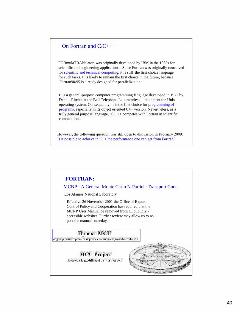
On Fortran and C/C++

FORmulaTRANslator was originally developed by IBM in the 1950s for scientific and engineering applications. Since Fortran was originally conceivedfor scientific and technical computing, it is still the first choice languagefor such tasks. It is likely to remain the first choice in the future, becauseFortran90/95 is already designed for parallelization.

C is a general-purpose computer programming language developed in 1972 by Dennis Ritchie at the Bell Telephone Laboratories to implement the Unix operating system. Consequently, it is the first choice for programming of programs, especially in its object oriented C++ version. Nevertheless, as atruly general purpose language, C/C++ competes with Fortran in scientificcomputations.

However, the following question was still open to discussion in February 2009:Is it possible to achieve in C++ the performance one can get from Fortran?

Effective 26 November 2001 the Office of Export Control Policy and Cooperation has required that the MCNP User Manual be removed from all publicly -accessible websites. Further review may allow us to re-post the manual someday.

MCNP - A General Monte Carlo N-Particle Transport Code

Los Alamos National Laboratory

FORTRAN:

41

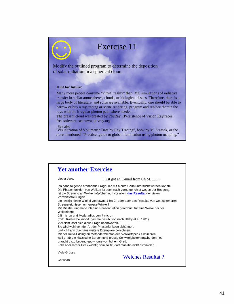
Exercise 11

Modify the outlined program to determine the deposition of solar radiation in a spherical cloud.

Many more people consume “virtual reality” than MC simulations of radiativetransfer in stellar atmospheres, clouds, or biological tissues. Therefore, there is a large body of literature and software available. Eventually, one should be able to barrow or buy a ray tracing or scene rendering program and replace therein the rays with the irregular photon path where needed ... The present cloud was created by PovRay (Persistence of Vision Raytracer),free software, see www.povray.org

“Visualization of Volumetric Data by Ray Tracing”, book by M. Sramek, or the afore mentioned “Practical guide to global illumination using photon mapping.”

See also

Hint for future:

Lieber Jaro,

Ich habe folgende brennende Frage, die mit Monte Carlo untersucht werden könnte: Die Phasenfunktion von Wolken ist stark nach vorne gerichtet wegen der Beugung. Ist die Streuung an Wolkentröpfchen nun vor allem das Resultat der vielenVorwärtsstreuungenum jeweils kleine Winkel von etwaq 1 bis 2 °oder aber das R esultat von weit seltenerenStreuuereignissen um grosse Winkel? Mit Miestreuung habe ich eine Phasenfuntion gerechnet für eine Wolke bei derWellenlänge0.5 micron und Moderadius von 7 micron (mittl. Radius bei modif. gamma distribution nach Ulaby et al. 1981). Vielleicht lässt sich diese Frage beantworten. Sie wird wohl von der Art der Phasenfunktion abhängen, und ich kann durchaus weitere Exemplare berechnen. Mit der Delta-Eddington Methode will man den Vorwärtspeak eliminieren, weil er für die klassische Berechnung grosse Schwierigkeiten macht, denn esbraucht dazu Legendrepolynome von hohem Grad. Falls aber dieser Peak wichtig sein sollte, darf man ihn nicht eliminieren.

Viele Grüsse

Christian

Yet another Exercise

Welches Resultat ?

I just got an E-mail from Ch.M. .........

42

The question could be formulated as follows:

Compare the MC results obtained with the exact phase function,with the phase function that is truncated at an angle θ 2 °(cosθ 0.999391 )

But we need also the mus!

I assume that the phase function provided as a table is in the form1

( )sin( )2

p d dθ θ θ φπ

p(θ) is tabulated

(cos ) ( )sin( )cp pθ θ θ=Here I plot as the function of cosθ

We could truncate at cos q = 0.99 and see what happens....

We shall sample cosθ

43

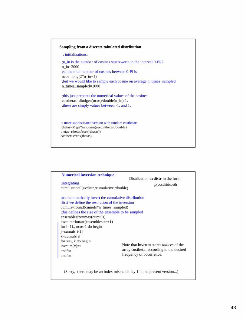
;n_in is the number of cosines stuetzwerte in the interval 0-Pi/2n_in=2000;so the total number of cosines between 0-Pi isncos=long(2*n_in+1);but we would like to sample each cosine on average n_times_sampledn_times_sampled=1000

;this just prepares the numerical values of the cosinescosthetas=dindgen(ncos)/double(n_in)-1.;these are simply values between -1. and 1.

Sampling from a discrete tabulated distribution

; initializations:

;a more sophisticated version with random costhetatsrthetas=Mypi*randomu(seed,nthetas,/double)thetas=rthetas(sort(rthetas))costhetas=cos(thetas)

;integratingcumuls=total(avdistr,/cumulative,/double)

;we nummerically invert the cumulative distribution;first we define the resolution of the inversioncumuls=round(cumuls*n_times_sampled);this defines the size of the ensemble to be sampledensemblesize=max(cumuls)invcum=lonarr(ensemblesize+1)for i=1L, ncos-1 do beginj=cumuls[i-1]k=cumuls[i] for x=j, k do begininvcum[x]=iendforendfor

Numerical inversion technique

(costh) costhp d

Distribution avdistr in the form

Note that invcum stores indices of thearray costheta, according to the desiredfrequency of occurrence.

(Sorry, there may be an index mismatch by 1 in the present version...)

44

rnd=round(randomu(thetaseed)*ensemblesize);chose the values from the prepared tablesindex=invcum[rnd]costheta=costhetas[index]

Sampling costheta values from the distribution

perhaps the costhetas table is not needed...