radio resource sharing and bearer service allocation for multi
TRANSCRIPT

RADIO COMMUNICATION SYSTEMS LABORATORY
Radio Resource Sharing and Bearer Service Allocation for Multi-Bearer Service,
Multi-Access Wireless Networks –
Methods to Improve Capacity
Anders Furuskär


RADIO COMMUNICATION SYSTEMS LABORATORY DEPARTMENT OF SIGNALS, SENSORS AND SYSTEMS
Radio Resource Sharing and Bearer Service Allocation for Multi-Bearer Service,
Multi-Access Wireless Networks –
Methods to Improve Capacity
Anders Furuskär
A dissertation submitted to the Royal Institute of Technology in partial fulfillment of the requirements for the degree of Doctor of Philosophy
May 2003
TRITA-S3-RST-0302
ISSN 1400-9137
ISRN KTH/RST/R--03/02--SE


iii
Abstract Two expected characteristics of future wireless networks are support for multiple bearer ser-vices, which in turn enable multiple end-user services, and the parallel use of multiple radio access technologies. This dissertation discusses radio resource management principles to im-prove capacity for such multi-bearer service, multi-access networks.
More specifically, it is first focused on how to most efficiently share the radio resource be-tween bearer service groups within one access technology. A general principle for sharing resources in interference limited systems is proposed, and its expected performance esti-mated. The proposed interference balancing principle maximizes capacity by adjusting the power budgets per bearer service group so that the maximum tolerable interference levels are equal for all bearer services. To verify its validity, the interference balancing principle is ap-plied to the 3rd generation cellular systems GSM/EDGE and WCDMA in a set of multi-bearer service case studies. It is seen that interference balancing may straightforwardly be introduced in these systems, and that significant capacity gains over non-balanced scenarios can be achieved.
Secondly, how to best share traffic load between the different sub-systems in a multi-access scenario is investigated. The capability to handle bearer services, and thereby also end-user services, typically differs between sub-systems. The overall multi-access system capacity is therefore affected by the allocation of bearer services on to sub-systems. Based on this, a simple principle for finding favorable, under certain constraints near-optimum, sub-system bearer service allocations is derived. It is seen that for a given service mix combined capaci-ties beyond the sum of the sub-system capacities may be achieved by using the favorable bearer service allocations. Significant capacity gains are also seen in a case study in which the bearer service allocation principle is applied to a combined GSM/EDGE and WCDMA multi-access system. The bearer service type may be said to reflect an expected radio re-source cost for supporting a user in each sub-system. By taking into account the actual radio resource cost, which may differ from the expected cost, when assigning users to sub-systems, further capacity gains are achievable.


v
Acknowledgements This dissertation exists thanks to the support of many people to whom I am most grateful. I first wish to thank my colleagues at the Radio Communication Systems Laboratory at the Royal Institute of Technology for valuable contributions. Especially acknowledged is the always relevant and accurate guidance from my main advisor Professor Jens Zander. I’m also most thankful for the valuable reviews and comments of Assistant Professors Tim Giles and Ben Slimane, as well as for the administrative assistance of Lise-Lotte Wahlberg.
The advising I’ve enjoyed from colleagues outside the Royal Institute of Technology, fore-most my industrial advisor at Ericsson Research Sverker Magnusson is greatly appreciated. The careful reviews provided by Magnus Frodigh, Harri Posti, and Birgitta Olin have also been of great value. Further, the many discussions with colleagues Magnus Almgren, Arne Simonsson, and Henrik Nyberg have contributed considerably to the material of this disser-tation. Moreover, the great deal I have learnt from working together with Peter de Bruin, Christer Johansson, Stefan Jäverbring, and Håkan Olofsson, together with the support of Tommy Ljunggren, have significantly aided in carrying out this work.
I wish to warmly thank Lovisa and my parents for love and encouragement.
Financing from the Swedish Research Council and Ericsson Research is of course greatly valued. At Ericsson the efforts of Håkan Eriksson, Magnus Madfors, and Sara Mazur associ-ated with this are well worth acknowledging.


vii
Contents
Chapter 1 Introduction 1 1.1 Multi-Bearer Service, Multi-Access Wireless Networks............................. 1 1.2 Related Work ............................................................................................... 4 1.3 Problem Formulation, Focus and Motivation .............................................. 7 1.4 Original Contributions ................................................................................. 9 1.5 Dissertation Outline ................................................................................... 12
Chapter 2 Multi-Bearer Service, Multi-Access Wireless Networks Fundamentals 13 2.1 Wireless Network Fundamentals ............................................................... 13 2.2 IMT-2000 Systems Service and Architecture Overview ........................... 15 2.3 Basic Radio Access Network Principles.................................................... 16 2.4 Multi-Access Wireless Networks .............................................................. 18
Chapter 3 System Models and Performance Measures 19 3.1 Performance Measuring and Modeling Approaches.................................. 19 3.2 Traffic Load and Service Mix.................................................................... 21 3.3 User and System-Level Quality ................................................................. 22 3.4 Multi-Bearer Service Quality, Capacity and Capacity Regions ................ 22 3.5 Normalized Measures ................................................................................ 23 3.6 Multi-Access Combined Capacity and Capacity Regions ......................... 25 3.7 Valuing Bearer Services............................................................................. 28
Chapter 4 Radio Resource Sharing in Multi-Bearer Service Interference Limited Wireless Networks 29
4.1 Per-Service Capacity Balancing ................................................................ 29 4.2 Interference Balancing ............................................................................... 33 4.3 Expected Performance ............................................................................... 36 4.4 Applicability of the Results ....................................................................... 45 4.5 Summary .................................................................................................... 47
Chapter 5 Multi-Bearer Service Case 1 – Voice and WWW in GSM/EDGE 49 5.1 GSM/EDGE Overview .............................................................................. 49 5.2 Interference Balancing in GSM/EDGE...................................................... 53 5.3 Models, Assumptions and Analysis Technique ......................................... 54 5.4 Numerical Results ...................................................................................... 63 5.5 Summary .................................................................................................... 69
Chapter 6 Multi-Bearer Service Case 2 – WCDMA with SIR-balancing Power Control 71
6.1 WCDMA Overview ................................................................................... 71

viii
6.2 Interference Balancing in WCDMA .......................................................... 74 6.3 Models and Assumptions........................................................................... 75 6.4 Numerical Results ...................................................................................... 78 6.5 Summary .................................................................................................... 81
Chapter 7 Multi-Bearer Service Case 3 – Voice and WWW in WCDMA/HSDPA 83 7.1 HSDPA Overview...................................................................................... 83 7.2 Interference Balancing in WCDMA/HSDPA............................................ 84 7.3 Models and Assumptions........................................................................... 85 7.4 Numerical Results ...................................................................................... 88 7.5 Summary .................................................................................................... 92
Chapter 8 Multi-Bearer Service Allocation in Multi-Access Wireless Networks 93 8.1 Information Availability Scenarios............................................................ 93 8.2 Bearer Service Allocation Strategies ......................................................... 94 8.3 Some Simple Illustrative Examples ........................................................... 98 8.4 Implementation Aspects........................................................................... 100 8.5 Applicability of the Results ..................................................................... 101 8.6 Summary .................................................................................................. 101
Chapter 9 Multi-Access Case 1 – GSM/EDGE and WCDMA/HSDPA 103 9.1 Underlying Results................................................................................... 103 9.2 Resulting Bearer Service Allocations and Capacity Regions .................. 104 9.3 Summary .................................................................................................. 106
Chapter 10 User Assignment in Multi-Access Wireless Networks 109 10.1 Additional System Models and Selection Variables................................ 109 10.2 Load Balancing ........................................................................................ 111 10.3 User Assignment Algorithms................................................................... 112 10.4 Expected Radio Resource Costs .............................................................. 115 10.5 Evaluation Methodology.......................................................................... 116 10.6 Numerical Results .................................................................................... 116 10.7 Summary .................................................................................................. 119
Chapter 11 Conclusions 123 11.1 How to Share Resources between Bearer Services?................................ 123 11.2 How to Allocate Bearer Services onto Sub-Systems? ............................. 124 11.3 Further Studies ......................................................................................... 125
References 127
Appendix A Abbreviations and Acronyms 137
Appendix B Asymptotic Behavior of Trunking and Diversity Gains 139
Appendix C The Effect of Requiring Equal Sub-System Qualities 147
Appendix D Per-Service Capacity and Interference Balancing Proofs 149

ix
Appendix E Additional GSM/EDGE Results 151
Appendix F Additional WCDMA/HSDPA Results 153
Appendix G A Graphical Method for Finding Near-Optimum Bearer Service Allocations 155
Appendix H Performance with Equal Service Mixes in Sub-Systems 157


1
Chapter 1 Introduction The use of wireless communications has undergone a tremendous growth over the past years. As of year-end 2002 there were a total of around 1.1 billion cellular subscribers worldwide. This number is expected to rise to about 1.8 billion by 2006 [1][2].
One technological factor that contributes to this growth is an increased number of bearer ser-vices1 offered by the wireless systems, which in turn enable an increased number of end-user services. Associated with this growth is also by necessity an improved capability of the wire-less systems to handle large numbers of users. This is partly enabled by development and deployment of new radio access technologies to be used in parallel with their predecessors. Two expected characteristics of future wireless networks are thus support for multiple bearer services and parallel use of multiple radio access technologies. This dissertation discusses sharing of radio resources between bearer services, and allocation of users of different bearer services onto radio access technologies for such networks.
In this introduction, an overview of multi-bearer service and multi-access networks is first given. Following this, previous work related to the problem area is reviewed. Next, defini-tions and motivations of the high-level problems studied in the dissertation are given. A sub-set of the high-level problem is also delimited, aiding in defining the scope of the disserta-tion. The main contributions of the dissertation are then summarized together with an over-view of the publications forming its basis. Finally, the outline of the dissertation is presented.
1.1 Multi-Bearer Service, Multi-Access Wireless Networks This section provides some background information on the emergence of the multi-bearer service and multi-access wireless networks focused on in this dissertation.
1.1.1 The Range of Offered Bearer Services is Increasing The number of bearer services offered by wireless networks is increasing. One example il-lustrating this is the evolution of cellular systems. The so-called 1st generation of cellular systems is exemplified by e.g. the Nordic Mobile Telephony system (NMT), the Total Ac-cess Cellular System (TACS), and the American Mobile Phone System (AMPS). These sys-tems offered access to the voice services of the Public Switched Telephony Network (PSTN). The 2nd generation of cellular systems includes systems like the Global System for Mobile Communication (GSM), US interim standards 95 and 136 (IS95 and IS136), and the Personal Digital Cellular system (PDC). When introduced, apart from providing capacity improvements compared to 1st generation systems, the 2nd generation systems also extended the range of bearer services to include moderate bitrate data bearer services (about 10kbps), supporting telephone modem traffic, and bearer services for simple end-user messaging ser-vices like the Short Message Service (SMS) of GSM. Since their introduction, many of the 2nd generation systems have, driven by the success of fixed Internet services, evolved to offer somewhat higher bitrate data bearer services (about 50-100kbps), both with guaranteed bi-trates and as best-effort bearer services without guarantees. Examples are High-Speed Cir-
1 A bearer service can be thought of as a ‘bit-pipe’ transferring the end-user service information over the wire-less part of the network. See Section 2.2 for a more precise definition of these terms.

2 Introduction
cuit Switched Data (HSCSD) and General Packet Radio Service (GPRS) for GSM and Cel-lular Digital Packet Data (CDPD) for IS136. The 3rd generation of cellular systems signifi-cantly increases the range of bearer services offered. In these systems, more formally de-noted IMT-2000 (International Mobile Telecommunications 2000) systems, in principle an arbitrary bearer service specified by attributes like bitrate, delay and error tolerance can be offered within the system capabilities (theoretically up to 2Mbps). The family of IMT-2000 systems includes e.g. Wideband Code Division Multiple Access (WCDMA), Enhanced Data-rates for GSM Evolution (EDGE) and Code Division Multiple Access 2000 (cdma2000). Improvements of 3rd generation systems offering even higher bitrates (exceed-ing 10Mbps) have also been standardized. These include the High-Speed Downlink Packet Access (HSDPA) concept for WCDMA and the High Data Rate (HDR) concept for cdma2000. When discussing a 4th generation of radio interfaces bitrates of 100Mbps are sometimes mentioned.
In parallel with the evolution of cellular systems, Wireless Local Area Networks (WLANs) have emerged as a complementary way to offer wireless bearer services. WLANs typically have high capacity, but a smaller range than cellular systems and thus require a larger num-ber of access points to cover a given area. Therefore, when used as a complement to cellular systems, WLANs are often used to cover spatial hot-spots in traffic demand. Examples of WLANs are IEEE802.11b and IEEE802.11a defined by the Institute of Electrical and Elec-tronics Engineers (IEEE) and the High Performance European Radio LAN 2 (HIPERLAN/2) defined by the European Telecommunications Standards Institute (ETSI).
The range of bearer services offered by wireless system has thus increased from only bearer service for voice to a multitude of bearer services. This multitude of bearer services brings about a large research area. Although a significant amount of work has been done in stan-dardization, defining multi-bearer service capable protocols, several challenges still remain. These include e.g. bearer service realization, i.e. selection of which of the often numerous alternative protocol modes provided by the standard to use to create bearer services fulfilling desired bitrates, delays and reliability requirements. Further, in principle the whole radio re-source management problem, allocation of communication port(s), waveform and power, may be revisited with bearer service type as a new dimension. In addition to solving these problems for each bearer service, how to share the full radio resource between bearer ser-vices needs to be determined.
1.1.2 Multiple Radio Access Technologies Will Co-exist
In parallel with the evolution and new development of radio access technologies, an ex-pected characteristic of future wireless networks is the cooperative use of a multitude of such radio access technologies in so-called multi-access networks. This expectation is motivated by the difficulty in designing one single radio access technology suitable for all possible ser-vices and deployment scenarios. In certain locations systems targeting wide coverage and mobility may be desired, which calls for certain system designs, whereas in other locations high bitrates and high capacity may be more critical issues, which possibly call for other de-sign choices. Further, the life spans of successive generations of radio access technologies with similar characteristics significantly overlap. Partly this is because deploying a new ra-dio access technology generation over a wide area is both time consuming and costly. Addi-tionally, in many cases the radio access technologies use designated frequency bands that are assigned to them long after the next generation is introduced. Finally, it may be noted that although global standardization efforts have aimed for one single radio access technology,

Introduction 3
this has not happened. Hence, different standards for systems with similar characteristics ex-ist.
An example of a multi-access network is depicted in Figure 1. In this example the included radio access technologies, henceforth denoted sub-systems, are GSM/EDGE, WCDMA and a WLAN (e.g. IEEE802.11b) sub-system. Other examples include other cellular technologies such as IS136, IS95, cdma2000, and future fourth generation radio access technologies, as well as broadcast technologies such as DAB and DVB and satellite networks. As discussed in [3], several alternatives exist regarding the relationships between the operators of the dif-ferent sub-systems. In this study, it is assumed that one single operator, or a set of co-operating operators, control all sub-systems, with the goal to reach a maximized or sufficient efficiency of the multi-access network as a whole. This is also the scenario expected to be most common in [3].
From an operator’s perspective, as indicated in Figure 1, sub-systems that are added to the multi-access network have the potential of improving the multi-access network’s coverage area, range of bearer services offered, or capacity. For a green-field operator, deploying a new system from scratch, also the cost for this may be lowered, e.g. by in each location de-ploying the sub-system most cost efficient for the traffic demand in question. Improving coverage and extending the range of offered bearer services are probably most important at an early stage, whereas improved capacity may be expected to become increasingly impor-tant at later stages, as the usage of the systems builds up. From an end-user perspective, im-proved coverage and range of bearer services offered are also beneficial, as well as poten-tially lower costs due to higher capacity and lower deployment costs of the operator. De-pending on the end-user service, a requirement from an end-user perspective may be seam-less, uninterrupted access to bearer services across different sub-systems. Not all of these goals may be deemed equally important; which goals are focused on depends on the strategy of the operator of the multi-access network. In addition to internal tuning of the sub-systems, the tools available to achieve the above goals include e.g. planning and deployment of the sub-systems and sub-system selection, i.e. which sub-system to select for a certain mobile station.
There are more requirements and challenges related to multi-access networks than those de-scribed above. One such challenge is selection of the architecture of the multi-access net-
WLANWCDMA GSM/EDGECoverage Capacity Services
WW
W W
W
W
W
G
G
G G
G
G
Figure 1. An example of a multi-access network.

4 Introduction
work, i.e. the way the different sub-systems are interconnected, such that the desired selec-tion procedures and seamless bearer services are supported. Another requirement is to have multi-mode capable terminals, possibly with parallel protocol stacks, the design and imple-mentation of which may be non-trivial. Alternatively, a user may use set of inter-working terminals, which poses requirements on cooperation between these.
1.2 Related Work A concept and architecture for handling mixed bearer services with different Quality of Ser-vice (QoS) requirements in wireless networks has been developed and standardized by the 3rd Generation Partnership Project (3GPP) [4]. A similar recommendation is provided by the International Telecommunications Union (ITU) in [5]. These concepts focus on specifying interfaces and procedures enabling negotiation and setting up of nearly any bearer services. However, how to realize the negotiated bearer services, i.e. a selection of which of the nu-merous protocol modes to use, as well as development of radio resource management algo-rithms to fulfill the negotiated bearer service requirements falls outside the scope of these standards and the related recommendations.
Within the area of radio resource management for mixed bearer services, several proposals have been published on how to maximize the utilization of a single communication link or a set of such links. These studies include e.g. Packet Reservation Multiple Access (PRMA) based solutions first proposed by Goodman et al. in [6]. This dissertation however targets interference limited scenarios, see further Section 2.1, for which maximized link utilization not always yields maximized capacity. One example of a system operating under interfer-ence limitation is a DS-CDMA uplink. For this specific case, several multiple bearer service studies have been made, proposing various radio resource management and sharing princi-ples as well as determining the performance of these. Initial results, limited to representing different bearer services by different radio link quality requirements, are presented by e.g. Guo et al. in [7], Sampath et al. in [8][9] and Mandayam et al. in [10]. These results are ex-tended, using more sophisticated models and assumptions, by e.g. Lee et al. in [11], adding different activity factors for different bearer services, and Park et al. in [12], taking power control errors into account. Other variations and extensions are presented in [13] - [17].
Among the DS-CDMA uplink studies, a generally applicable principle is also given by Wang and Aghvami in [18] and [19]; stating that Quality of Service (QoS) balancing be-tween bearer services should maximize capacity. This is then applied to a DS-CDMA uplink, for which a power allocation scheme achieving QoS balance is derived. However, a more general method for how to balance QoS is not given. Similar to Wang and Aghvami’s QoS balancing principle, it has also been proposed by Sampath et al. in [8] that for a DS-CDMA uplink, at a capacity-wise optimal power allocation per user, all QoS constraints are met with equality. A related proposition is further made by Park et al. in [12].
All the DS-CDMA uplink studies [7] - [17] above report a linear relationship between the numbers of supportable users of different bearer services.
The DS-CDMA downlink is somewhat more complex to analyze analytically, and fewer studies have been published. Zhang and Choi et al. have however presented mixed voice and data capacity evaluations in [20] and [21] respectively. In both cases non-linear relationships between the numbers of supportable users of different bearer services are shown. No general multi-bearer service principles or performance analyses for FDMA or TDMA based systems have been found in the literature.

Introduction 5
Turning to analyses of systems standardized for commercial operation, a few mixed bearer service investigations for GSM and standard GPRS have been done in the past. Bianchi et al. [22] have evaluated GPRS access delays in mixed voice and data systems for fixed and dy-namic resource allocation schemes, and have shown that reserving a few channels for GPRS usage may considerably decrease such delays. Ni et al. [23] have evaluated the impact of GPRS traffic occupying unused voice channels on voice outage probability, and concluded that this depends on frequency reuse (i.e. to which extent the system is interference vs. blocking limited). The results are also expressed as a reduction in voice coverage due to the introduction of interference from data users. Jacobsmeyer presents a similar analysis for IS136 in [24], estimating the voice coverage loss per admitted data stream. Ni et al. [25] have also evaluated the mean GPRS queuing time as a function of offered GPRS traffic in a system with fixed offered voice traffic [25]. Stuckmann et al. [26] and Mahdavi et al. [27] have performed similar analyses. Stuckmann includes more GPRS protocol details. These innovative papers can however typically be said to focus on either one of the bearer services studied, voice or data, and see the other as a source of interference. The above studies typi-cally focus on a fixed bearer service mix, and do not derive relationships between the num-bers of users of different bearer services supportable by the systems. In addition to the publi-cations related to this dissertation, more recently Rodriguez et al [28], Salmenkaita et al. [29], and Gimenez et al. [30] have presented power control and dynamic frequency and channel assignment concepts for GSM/EDGE systems with mixed voice and data bearer ser-vices. In these studies, the quality of both bearer service types is considered and capacity is evaluated for a range of service mixes. Significant capacity gains are reported.
For WCDMA and CDMA2000, a few mixed bearer service studies may also be found. Bearer design and performance for mixed voice and interactive data bearer services in WCDMA is for example discussed and evaluated by De Bernardi et al. in [31] and Imbeni and Karlsson in [32]. Zhang et al. further target UMTS-like systems’ uplinks and downlinks in [33] and [20] respectively. IMT2000 systems are analysed by Song in et al. in [34]. A mixed voice and data performance evaluation of cdma2000 is provided by Lim in [35]. Fu-ruskär et al. have analyzed the performance of mixed voice and data bearer services in WCDMA/HSDPA in [93]. Among these applied studies, linear relationships between the number of supportable users of different bearer services is reported in [31], [32], [34] and [35], whereas non-linear relationships are found in [20] and [33].
Typical for the above multiple bearer service studies is that they, by necessity take a great level of details into account, and hence provide radio resource management solutions and performance estimations applicable for rather specific scenarios or systems. In addition to these very valuable specific results, somewhat more general radio resource management principles or guidelines that can be used to share resources between bearer services and es-timate performance for larger sets of systems are desirable. Apart from what is proposed by Wang and Aghvami in [18] and [19], and the related observations by Sampath et al. in [8] and Park et al. in [12], no such principles have been found in the literature however.
Several interesting multi-access concepts may be found in the literature. In the report of the scenario project Wireless Foresight [36], Karlsson et al. discuss different possible scenarios for the wireless world in 2015. In all four scenarios, heterogeneous infrastructures consisting of a variety of radio access technologies are foreseen. This conclusion is motivated in an early paper by Katz et al. [37], in which an overlaid architecture of different sub-systems is proposed, based on strengths and weaknesses of homogeneous, single-access networks. Fro-digh et al. describe a so-called always-best-connected concept comprising GSM/EDGE,

6 Introduction
WCDMA, CDMA2000 and WLAN access technologies, as a candidate for a future genera-tion wireless network in [38]. A related future wireless infrastructure is foreseen by Bria et al. in [39]. Walke discusses similar trends in [40], partly concluding that “…multiple radio interfaces competing worldwide to serve the same applications will continue to exist in the future…”. Honkasalo et al. focus on the inter-working of WCDMA and WLAN in [41], pro-posing WLAN as a hotspot complement to WCDMA for cellular operators. Other multi-access concept descriptions include Varshney et al. [42], who associate multi-access net-works with 4th generation wireless systems. Further, an architectural and functional frame-work, including a function for service mapping on to radio access technologies, for so-called composite networks is described by Demestichas et al. in [43] and [44], and by Papadopou-lou in [45]. Strategies for transparently, i.e. regardless of which access networks is used, providing users with services in multi-access systems is discussed by Daoud et al. in [46]. Convergence of the cellular and WLAN networks with broadcast networks such as DAB and DVB is further covered by the European Commission driven Information Society Technolo-gies (IST) Dynamic Radio for IP-Services in Vehicular Environments (DRiVE) project [47], and its follow-up project Over-DRiVE [48]. The outcome of these projects includes propos-als for multi-access system architectures and requirements on system functionality, compris-ing e.g. dynamic spectrum sharing and traffic control between the radio access technologies. Such results have been presented e.g. by Keller et al. in [49], Walsh et al. in [50], and Tönjes et al. in [51].
A number of multi-access investigations on a more detailed level than the above conceptual studies may also be found in the literature. Analyses of the single-bearer service trunking gain enabled by the larger resource pool resulting from combining such systems have been presented e.g. by Tölli et al. in [52] and Heickerö et al. in [53]. Tölli et al. have also investi-gated how to maintain this trunking gain with a limited amount of inter-system handovers in [54].
In related studies, Linke-Salecker and Hood investigate the reduction in blocking achievable by combining separate 2nd and 3rd generation networks into one multi-access network. Dif-ferent system overflow mechanisms for voice bearer services are investigated for different rates of multi-mode capable terminals in [55]. In [56], the concept is extended to cover voice and circuit switched data bearer services, and it is recommended to load the 2nd generation network with as many voice users as possible in order to make room for data users in the 3rd generation network. In [57], the capacity not used by circuit switched bearer services is also measured, estimating the capacity potential of a packet switched bearer service, which is seen to be affected by the overflow mechanism.
Alexandri et al. [58] have attacked the complex problem of assigning users of different bearer services onto different radio access technologies using Reinforcement Learning (RL). Their proposed RL-based assignment scheme manages to increase resource utilization over allocating users the relatively least loaded radio access technology. In [59], Kalliokulju et al. discusses the similar problem of radio access selection for multi-standard terminals. They compare capacity, coverage and delay among different sub-systems, and discuss how these can be used for access selection. The conclusions include that WLAN should be used for high data rate applications, whereas cellular technologies should be used for moderate bitrate applications and mobile users.
The problem of supporting handovers between different sub-systems has also been given some attention in the literature. This problem may be studied and solved on different proto-

Introduction 7
col levels. An overview of issues related to handover in multi-access systems is provided by Pahlavan et al. in [60]. The term vertical handoff, meaning handoff between sub-systems in a multi-access system, was introduced and evaluated by Stemm and Katz in [61]. A user-policy-based handover principle that allows users to connect to the sub-system that is pre-ferred according to individual price and performance preferences is proposed by Wang et al. in [62]. In [63], Gwon et al. propose mechanisms for improving the Mobile Internet Protocol (Mobile IP) to enable seamless handovers for real-time services between sub-systems, in-cluding 3G, GPRS and WLAN. Enhanced Mobile IP-based solutions for handover between UMTS/GPRS and WLAN are also proposed by Bria et al. in [39]. Common Radio Resource Management (RRM) procedures, including handover and cell reselection, for combined GSM/EDGE and WCDMA are presented by the 3rd Generation Partnership Project (3GPP) [64][65]. These also include means for exchanging traffic load and quality information be-tween sub-systems to enable bearer service and load-based assignment of users. Some of these principles are also described by Virtej et al. in [66] with a focus on the associated modifications the GSM/EDGE radio access network.
Supporting QoS over multi-access systems for which different sub-systems may offer and manage QoS in different and incompatible ways is discussed by Jain and Varshney in [67].
Finally, the problem of implementing multi-mode terminals for multi-access systems has been addressed e.g. by Harada et al. in [68], where they propose a protocol stack capable of seamless communication over multiple sub-systems. Software defined radios are an attrac-tive approach to implementing multi-mode terminals. Mitola provides an overview of soft-ware defined radios in [69]. Ogose further discusses the application of software defined ra-dios in multi-access 2nd and 3rd generation systems, and the need for automatic mode selec-tion in [70]. In [71], Mitola et al. also extend the software radio concept to so-called cogni-tive radio, in which self-aware radios can control several radio aspects, including selection of sub-system.
Multi-access systems have only since quite recently been treated in the literature. They do however show some resemblance with some other system concepts, e.g. multi-frequency band systems, dual mode analog and digital systems, as well as systems with Hierarchical Cell Structures (HCS). Analysis of dual mode systems is covered e.g. by Kakakes in [72] and by Ramésh and Balachandran in [73]. Radio resource sharing in HCS systems is covered e.g. by Karlsson in [74]. These results are however not directly applicable to multi-access systems, for which the resources of sub-systems are independent of each other, which is not the case for dual-mode and HCS systems where the sub-systems compete for the same radio resource. The capacity of a multi-frequency band GSM 900MHz and 1800MHz network is evaluated by Tegler et al. in [75], showing significant capacity gains of the combined system over the 900MHz-only network. Similar results may be expected for multi-access systems.
With regard to the multi-access related scope of this dissertation, it is noted that the capabil-ity to handle bearer services typically differs between sub-systems in multi-access networks. No previous studies have been found explicitly taking the relationship between the numbers of supportable users of different bearer services in different sub-systems into account when allocating users of different bearer services to sub-systems.
1.3 Problem Formulation, Focus and Motivation On a high level, the goal of this dissertation may be formulated as achieving high capacity for multi-bearer service, multi-access wireless networks. This would correspond to the desire

8 Introduction
of an operator of a rather mature network with satisfactory current coverage and set of bearer services offered. Several methods to improve capacity exist, ranging from physical layer to application layer improvements, and also including planning and deployment enhancements. This dissertation focuses on improvements in capacity specific to multi-bearer service and multi-access networks.
For any multi-bearer service network, a problem that must be dealt with is that of radio re-source management for multiple bearer services. This problem may be split into two sub-problems: (i) how to share the radio resources between groups of users of different bearer services, and (ii) how to manage radio resource budgets within each such bearer service group? The latter sub-problem may in principle be solved as in the single-bearer service cases. In some cases more efficient multi-bearer service-adaptive solutions may indeed exist, e.g. scheduling data in-between voice ‘talk spurts’. However, finding such solutions is not the main focus of the dissertation. Instead, the focus is on the former of the sub-problems. With this focus, the first dissertation problem may be reformulated as:
P1) Within one sub-system, how should radio resources be shared between bearer ser-vices for maximum capacity?
A further focus of the scope is made possible by the observation that capacity is typically limited by the number of available communication channels, e.g. frequencies, time slots or spreading codes, and the quality of these channels, e.g. in terms of carrier-to-interference ratios. In many cases, the highest capacity is achieved under interference limited operation, where the availability of channels does not limit the performance of the system. Based on this, the dissertation studies mainly interference limited scenarios.
Despite these limitations, solutions to the problem are desired that are more generally appli-cable, i.e. for arbitrary interference limited networks, than the case-specific solutions [7] - [35] described in the previous section. Additionally, it should be noted that the split of the multi-bearer service radio resource management problem into radio resource sharing be-tween bearer services and radio resource management within bearer service groups may ren-der sub-optimal performance if fixed resource budgets per bearer service-group are used, for which cases trunking losses may occur. Therefore, dynamic resource sharing principles are targeted.
An outcome of studying problem P1 is that different bearer services fit and mix differently in different sub-systems. For any multi-access network, the problem of how to best share the overall traffic load between different networks emerges. This also constitutes the second dis-sertation problem:
P2) With multiple sub-systems at hand, how should the traffic load be shared between these for maximum capacity?
How to best do this, and the resulting performance, depends on the amount of information available across the different sub-systems, and when this information is available. This dis-sertation addresses different such scenarios, ranging from no to full information availability across the sub-systems. The focus is on the case where the bearer service type of users is known across the systems. Apart from potentially large capacity gains, the motivation for this is that information on the bearer service type is relatively easy to establish and may be conveyed between sub-systems with very limited signaling bandwidth. Additionally, as op-posed to e.g. a user’s current radio link quality, it typically does not change frequently with time, which further reduces the signaling bandwidth requirements.

Introduction 9
The basic motivation for studying these problem areas is that, as discussed in Section 1.1, multiple bearer services and use of multiple radio access technologies are expected to be im-portant characteristics of future wireless networks. With capacity as a performance measure, the focus may be further motivated as adhering to the vision of “Affordable Wireless Multi-media and Infrastructure” of the Center for Wireless Systems at KTH [76]. Assuming that the cost per user decreases with the system capacity, multimedia services are made afford-able by high-capacity radio resource sharing for mixed bearer services and high-capacity traffic load sharing between the different sub-systems of the infrastructure.
1.4 Original Contributions With the focus discussed in the previous section, the aim of the dissertation is to first derive general solutions to the stated problems P1 and P2, which are then verified in a number of case studies. More specifically, the following contributions are made addressing problem P1:
C1a) Introduction of the interference balancing concept, including its applicability, as a general method for maximizing capacity in interference limited multi-bearer service networks
C1b) Development of a framework for predicting and explaining the multi bearer service capacity in interference limited networks.
These general principles are then verified in a number of case studies:
C1c) Maximizing mixed voice and interactive data capacity for GSM/EDGE-based sys-tems through service-based power setting, which is a form of interference balancing.
C1d) Maximizing mixed bearer service capacity in DS-CDMA-based systems through bal-ancing maximum output powers with respect to Signal-to-Interference Ratio (SIR) targets, which is a form of interference balancing.
C1e) Evaluating mixed voice and interactive data capacity for WCDMA/HSDPA-based systems and improving it through interference balancing.
Turning to the multi-access problem P2, the following contributions are made:
C2a) Development of a simple method for finding sub-system bearer service allocations that maximize combined capacity in a multi-access network.
C2b) Application and verification of the above principles to multi-access GSM/EDGE and WCDMA networks.
C2c) Development and comparison of a set of multi-access user assignment algorithms including random access selection, bearer service-based access selection, cost-based access selection, and cost and bearer service-based access selection.
In summary, C1a-e and C2a-c are the contributions made to solving problems P1 and P2 re-spectively. Further, in addition to these contributions, a general prerequisite for solving the problems, which may also be regarded a contribution, is:
C0) Establishment of system models and performance measures for evaluation of multi-bearer service multi-access wireless networks.

10 Introduction
1.4.1 Included Publications For each contribution, this section lists a number of publications in which the dissertation material has previously been presented. Much of the material has been published in papers written together with other authors. Therefore, a rough opinion, agreed between the authors, is given of this author’s contributions to the material in the publications. The contributions are where appropriate divided into conceptual (e.g. ‘use of higher layer modulation’) and performance evaluation (selection of system models and definition of performance measures etc.).
Contribution C1a has earlier been published in short form together with case studies relating to contributions C1c and C1e. Contribution C1b in its general form is published for the first time in this dissertation. Publications including contribution C1c are:
1. A. Furuskär, P. de Bruin, C. Johansson and A. Simonsson, ‘Managing Mixed Services with Controlled QoS in GERAN – The GSM/EDGE Radio Access Network’, IEE 3G Mobile Communication Technologies 2001 [77]. Contains derivation of principles for handling arbitrary mixed bearer services with controlled QoS and system performance analysis of mixed voice and interactive data bearer services in GERAN. This author is responsible for the development of the QoS controlling principles and the performance evaluation.
2. A. Furuskär, P. de Bruin, C. Johansson and A. Simonsson, ‘Mixed Service Management with QoS Control for GERAN – The GSM/EDGE Radio Access Network’, IEEE VTC’2001 spring [78]. Contains further evaluations of the above QoS controlling princi-ples, including power controlled voice bearers. Contributions as for publication 1.
3. A. Furuskär, P. de Bruin, C. Johansson and A. Simonsson, ‘Controlling QoS for Mixed Voice and Data Services in GERAN – The GSM/EDGE Radio Access Network’, IEEE 3G Mobile Communications [79]. Contains evaluations of the above QoS controlling principles for different classes of interactive data bearer services, also verifies the power setting concept for three different bearer services. Contributions as for publication 1, but with Mr. Simonsson responsible for half of the performance evaluation.
4. P. de Bruin, S. Craig and A. Furuskär, “A Simple High Capacity Multiple Service Solu-tion with Controlled QoS for GERAN”, IEEE VTC’02 Spring [80]. Proposes and evalu-ates a comprehensive RRM solution for mixed bearer service GSM/EDGE systems. This author provided the Service-Based Power Setting principle and the overall system per-formance evaluation, as well as contributed to the Power-Based Admission Control prin-ciple. The idea of combining the three techniques tight frequency reuse, Service-Based Power Setting and Power-Based Admission Control were contributed to equally by all the authors.
Although the results are not explicitly included in this dissertation, the mixed bearer service GSM/EDGE contribution C1c relies on a number of single bearer service concepts and per-formance analyses. These have been published in e.g.:
5. A. Furuskär, M. Frodigh, H. Olofsson and J. Sköld, ‘System Performance of EDGE, a Proposal for Enhanced Data Rates in Existing Digital Cellular Systems’, IEEE VTC’98 [81]. Contains first system performance evaluation of the then preliminary EDGE con-cept, which is basis for the ITU IMT-2000 application. This author provided the per-formance evaluation. The conceptual material was provided equally by the four authors.

Introduction 11
6. S. Eriksson, A. Furuskär, M. Höök, S. Jäverbring, H. Olofsson, and J. Sköld, ‘Compari-son of Link Adaptation Strategies for Packet Data Services in EDGE’, IEEE VTC’99 [82]. Proposes and evaluates, on link level, the later standardized combined link adapta-tion and incremental redundancy link layer for GSM/EDGE. The concept was contrib-uted to roughly equally by the authors.
7. A. Furuskär, D. Bladsjö, S. Eriksson, M. Frodigh, S. Jäverbring and H. Olofsson, ‘Sys-tem Performance of the EDGE Concept for Enhanced Data Rates in GSM and TDMA/136’, IEEE WCNC’99 [83]. Contains the first system-level performance evalua-tion of the EDGE concept including the incremental redundancy link layer functionality discussed above. This author contributed to the concept and provided the performance evaluation.
8. A. Furuskär, ‘Statistical QoS Requirements, Timeslot Capacity and Dimensioning for Interactive Data Services in GERAN – The GSM/EDGE Radio Access Network’, NRS’2001 [84]. Contains an analysis of the impact of different system scenarios and ra-dio environments on system performance for GSM/EDGE interactive data bearer ser-vices and derivation of simple dimensioning principles for GSM/EDGE data bearer ser-vices. This author sole contributor.
9. M. Eriksson, A. Furuskär, M. Johansson, S. Mazur, J. Molnö, C. Tidestav, A. Vedrine and K. Balachandran, “The GSM/EDGE Radio Access Network – GERAN; System Overview and Performance Evaluation”, IEEE VTC2000 Spring [85]. Proposes and evaluates the later standardized modular design of the GSM/EDGE radio interface. The concept was contributed to roughly equally by all the authors.
10. A. Furuskär, “Can 3G Services be offered in Existing Spectrum?”, licentiate thesis [86]. Contains most of the above GSM/EDGE results.
Variations of the above studies have also been published in [87], [89], [90] and [91].
Contribution C1d is published for the first time in this dissertation. Contribution C1d has previously been published in:
11. S. Parkvall, J. Peisa, A. Furuskär, M. Samuelsson and M. Persson, “Evolving WCDMA for Improved High Speed Mobile Internet”, FTC’2001 [92]. Proposes and evaluates RRM principles for handling single and multiple bearer services when the High-Speed Downlink Packet Data bearers are introduced in release 5 of the WCDMA standard. This author contributed with the mixed bearer service principles and performance evaluation.
12. A. Furuskär, S. Parkvall, M. Persson, and M. Samuelsson, “Performance of WCDMA High Speed Packet Data”, IEEE VTC’02 spring [93]. As publication 11, but with refined models and assumptions. This author again contributed with the mixed bearer service principles and performance evaluation.
The multi-access related contributions C2a-c have in part previously been published, or are planned to be published, in the following papers:
13. A. Furuskär, “Multi-Service Allocation for Multi-Access Wireless Networks”, IEEE MWCN 2002 [94]. Proposes and evaluates principles for allocating multiple bearer ser-vices on to different sub-systems in multi-access systems.
14. A. Furuskär and J. Zander, “Multi-Service Allocation for Multi-Access Wireless Net-works”, submitted for IEEE Transactions on Wireless Communications [95]. As

12 Introduction
MWCN’2002. Content as for MWNC 2002 but generalized for arbitrary number of bearer services and sub-systems. This author has contributed with both concepts and analysis.
Despite being used in most of the above publications, the material relating to contribution C0 is published in detailed for the first time in this dissertation.
1.5 Dissertation Outline The dissertation outline is intended to match the problem definition. Following this introduc-tion, Chapter 2 continues with an overview of the systems studied, including e.g. service, architecture and protocol aspects. Chapter 3 discusses how these systems are modeled and how their performance is measured.
How to share resources between bearer services (P1) is discussed in Chapter 4 - Chapter 7. General principles and expected capacity results for interference limited networks are first developed and discussed in Chapter 4. These principles are then applied and their perform-ance verified in three different case studies. A GSM/EDGE system with mixed voice and WWW bearer services is studied in Chapter 5, a power controlled WCDMA system with mixed SIR-targets is studied in Chapter 6, and a WCDMA/HSDPA system with mixed voice and WWW bearer services is studied in Chapter 7.
Allocation of different bearer services onto multiple sub-systems in multi-access networks (P2) is discussed in Chapter 8 - Chapter 10. In Chapter 8, general bearer service allocation principles are derived for the case where the only decision parameter is the bearer service type. In a case study in Chapter 9 these principles are then applied to combined GSM/EDGE and WCDMA multi-access networks, assuming a set of different sub-system capabilities. Chapter 10 extends the user assignment principles of Chapter 8 by also taking the actual ra-dio resource cost of users into account when assigning them to sub-systems. Some examples indicating the potential gain of this are also given.
The main conclusions of the dissertation are given in Chapter 11, together with recommen-dations for further studies. Material not directly related to answering the two problems P1 and P2 are placed in appendices.

13
Chapter 2 Multi-Bearer Service, Multi-Access Wireless Networks Fundamentals
This chapter contains a simplified review of some fundamental wireless network concepts, as well as gives an overview of the services, architecture and functionality of the wireless networks studied in the case studies of this dissertation. These aspects of the networks are in large assumed to adhere to the recommendations on IMT-2000 systems issued by the ITU. The networks may hence be regarded IMT-2000-like2.
The intention of this chapter is to provide the minimum necessary background for under-standing both the general performance measures and requirements defined in Chapter 3, and the specific additions used in the case studies. To limit the extent of this background infor-mation, sometimes overly simple reasoning is used, and details skipped. Precise definitions of the models and assumptions used in the dissertation are provided in Chapter 3 and in the case study chapters. More detailed background material may be found in the references given throughout the text.
2.1 Wireless Network Fundamentals This section reviews some fundamental principles of wireless system design. A more thor-ough presentation may be found in e.g. [96].
To connect mobile users to the services of a fixed network, radio channels are used. These radio channels convey information between Mobile Stations (MSs) carried by the users and Base Stations (BSs) connected to the fixed network. One single MS may use multiple chan-nels. The number of channels used depends e.g. on the (bearer) service type. It is also possi-ble for multiple MSs to dynamically share channels. Such shared channels are often referred to as packet switched channels.
Due to radio propagation characteristics, limitations in output power, and noise, some of which generated in the radio receivers, the range of a base station is limited. At distances be-yond the range limit the received signal power PS is too small in comparison to the noise power PN for the signal to be distinguishable from the noise. The area covered by a base sta-tion is often denoted a ‘cell’. The location of a base station is denoted a ‘site’. Sometimes multiple base stations with differently directed coverage areas are co-located at one site. The coverage area of each such base station is denoted a ‘sector’.
To cover a larger area than that of one cell, multiple base stations need to be deployed. A wireless system typically is assigned a finite frequency spectrum. Within this spectrum a limited number Ctot of orthogonal radio channels, i.e. channels that do not interfere with each other, may be found. This holds regardless of whether the channels are divided in time as in Time Division Multiple Access (TDMA) systems, in frequency as in Frequency Division Multiple Access (FDMA) systems, or with spreading codes as in Code Division Multiple Access (CDMA) systems. The number of orthogonal channels that may be found further de-pends on the bandwidth of the channels. The limited number of orthogonal channels means 2 This does not mean that the results of this thesis do not apply to other types of wireless networks. Further dis-cussions on the applicability of the results are provided in connection with their derivations.

14 Multi-Bearer Service, Multi-Access Wireless Networks Fundamentals
that eventually, to cover a large area, radio channels have to be reused in several base sta-tions. The reuse of radio channels introduces interference in the system, which reduces the ability to receive the desired radio channel. The more frequently the radio channels are re-used, the higher the received interference power PI, and the harder it becomes to detect the desired radio channel. At the same time, the more frequently the radio channels are reused, the more channels are available per base station, and the more users can be assigned their desired set of channels, or the more often they can access shared channels. Assuming that each channel is reused in every Kth base station, the number of channels per base station is given by CBS = Ctot/K. How frequently the radio channels can be reused is determined by the ability of the radio receivers to distinguish the desired signal from the interfering signal. This is often measured in terms of a minimum required Signal-to-Interference Ratio, SIR = PS / PI. Figure 2 depicts an example of a multi cell network with reused radio channels.
As noted above, the coverage area of a wireless system is limited to regions where the re-ceived signal power PS is sufficiently high in comparison to the noise power PN. Within the coverage area, for a given distribution of the number of channels required per user, the num-ber of users per base station UBS supported by the system, or the system capacity, is limited by the number of channels available per base station CBS and/or the increased interference levels from neighboring base stations. A system for which the number of users is limited by the amount of available channels is denoted blocking limited or channel limited. In this case, if the average number of channels per users is Cuser (note that Cuser < 1 is possible with shared channels), the maximum number of user per base station is given by UBS = CBS / Cuser. In case the bearer service is such that users queue for a free channel upon entering the sys-tem when no free channels are available, which is often the case with shared channels, these types of systems are sometimes denoted queuing limited. When the number of users per base station increases, the received interference power PI also increases. When PI reaches a suffi-ciently high level in comparison to PS, the desired signal is no longer satisfactory detectable, and the quality of the radio link becomes unacceptable. A system which reaches this state before the number of users per base station multiplied with the average channel usage reaches the number of available channels, i.e. for some UBS < CBS / Cuser, is denoted interfer-ence limited. A system for which the received signal power PS is not sufficiently high in comparison to the noise power PN is denoted noise limited or range limited. Most systems are noise limited in some area regions, e.g. at the system periphery. Systems with high reuse factors have a long distance to interferers and few channels per base station, and are typically blocking limited. Systems with small reuse factors on the other hand yield short distances to interferers and many channels per base station, and typically become interference limited. It
M SB SCell P I
Chi
Chi
Chi+1
Chi+2
Chi+1
Chi+3
Chi+4
P S
Figure 2. Several cells are used to cover a large area. Cells that use the same set of radio channels (Chi) may interfere with each other.

Multi-Bearer Service, Multi-Access Wireless Networks Fundamentals 15
should be noted that in practice many systems are limited by a combination of blocking, in-terference, and coverage.
From a performance perspective, interference limited systems typically enable higher capaci-ties than blocking limited systems. This is because unless blocking limited systems can be designed so that PI reaches its maximum level for UBS = CBS / Cuser, higher capacities can be achieved by lowering the reuse factor, thereby increasing CBS, until the system becomes in-terference limited. A drawback with interference limited networks is that the when the num-ber of users in the system exceeds the capacity limit, which may happen because channels are available, the quality of the radio link become poor. To prevent this some form of admis-sion control is required, which limits the number of users in the system to numbers for which interference levels are acceptable. With the motivation of the higher capacity enabled by in-terference limited systems, these are therefore the type of networks focused on in this disser-tation.
The above discussion is applicable to FDMA, TDMA and CDMA systems, and combina-tions thereof. In practice however, especially CDMA systems with other frequency reuse factors than 1 are rare, although code reuse in principle is possible. Also newly deployed FDMA/TDMA systems, foremost represented by GSM, tend toward using as low reuse fac-tors as 1. The motivation for this is the higher capacity potential.
2.2 IMT-2000 Systems Service and Architecture Overview Figure 3 depicts a simplified view of the system and bearer service architecture of IMT-2000 cellular systems defined in [4] and [5]. For conveying end-to-end information, end-user ser-vices, or applications, make use of end-to-end bearer services. These end-to-end bearers are in turn realized using bearer services of the networks included in the end-to-end link. Note that there need not be an explicitly defined end-to-end bearer, in which case the end-to-end bearer is instead implicitly specified by the bearer services of the included networks. In this chain of bearer services, the IMT-2000 systems offer bearer services between mobile users and fixed interface points at which the IMT-2000 systems are connected to different external networks. These bearers are denoted IMT-2000 bearers in Figure 3. Examples of external networks are the Public Switched Telephony Network (PSTN) and the Internet. The IMT-
IM T-20 0 0 Bearer
M S
Rad io A cces s Bearer
Rad io Beare r
BS BS C/ R NC
Ra di o Acces s Network
En d -to -en d Serv ice
C N g ateway
C N ed g e n o deSe c tor
Se c tor
Se c tor
Core Netwo rkInterne t
PS TN
Figure 3. Simplified schematic IMT-2000 bearer service and system architecture.

16 Multi-Bearer Service, Multi-Access Wireless Networks Fundamentals
2000 bearer services are characterized by QoS profiles, which comprise a list of attributes such as bitrates, delays, and bit error rate requirements, see further [4] and [5].
Internally, an IMT-2000 system is divided into a Core Network (CN) and a Radio Access Network (RAN). The CN interfaces to, and handles requests for bearer services from, the external network and mobile users. The CN further keeps track of where mobiles are located and routes information to the correct RAN. The CN realizes its offered bearer services through requesting suitable Radio Access Bearer (RAB) services from the RAN. The RAN in turn realizes these RAB services by configuring the protocols of its radio interface in a proper way, thereby creating a so-called Radio Bearer (RB). Through employing various Radio Resource Management (RRM) techniques, the RAN also maintains a radio link qual-ity sufficient for fulfilling the requirements of the requested QoS profile. The RAN is typi-cally further divided into Base Stations (BS) and Base Station Controllers (BSC). As dis-cussed in the previous section, the base stations, containing the radio transmitters and receiv-ers, are geographically deployed to maximize a combination of coverage, capacity and qual-ity for a given cost. A typical deployment approach is to co-locate a number base stations at a site, with each base station covering one sector of the full coverage area of the site.
2.3 Basic Radio Access Network Principles Some fundamental principles for transmitting voice and data information through the radio access network are depicted in Figure 4. A telephone conversation, or a call, typically con-sists of the involved parties taking turns in speaking. Studying the voice flow in one direc-tion this then appears as a sequence of talk spurts separated by silence periods. For voice calls originating from the PSTN, during a talk spurt information arrives at the radio access network in form of a constant rate flow of speech frames originating from the speech coder. For voice calls originating from the Internet the arrival rate may vary because of non-constant frame delays. The frame size, frame duration and frame arrival rate further depend on the speech coder; typical values are 30 bytes, 20ms and 50 frames per second. Before sending the speech frames over the radio interface the radio access network may process them. This processing may include e.g. trans-coding, i.e. change of source code, as well as channel coding. In the systems studied in this work, due to the stringent delay requirements no buffering of speech frames is done. The requirements on low delay also prevent retrans-mission of erroneous speech frames. Further, due to the relatively high voice activity factor, each voice flow is typically allocated a dedicated, or circuit-switched channel. The number of dedicated channels supported by the radio access network is limited. When this limit has been reached, if the number of channels required per call cannot be reduced by applying an alternative source code, no more calls can be accepted and new call attempts are blocked. It should be noted that buffering and retransmission of speech frames as well as using statisti-cally multiplexed shared channels is perfectly possible. These techniques are however typi-cally not used in the IMT-2000-like systems of the case studies of this dissertation. Further, buffering of speech frames and statistical multiplexing reduces blocking. Blocking does not occur in the interference limited systems, which are the focus of this dissertation, and there-fore inclusion of these mechanisms would not increase capacity. For GSM-like systems this is further discussed in [97]. For accepted calls a satisfactory speech quality should be main-tained. This quality can be estimated by the rate of bit errors or the rate of lost or erased frames over the radio interface. Calls with low voice quality may be dropped from the sys-tem to free up radio resources. The task of the radio access network may be summarized as supporting as many calls as possible while maintaining an acceptable voice quality.
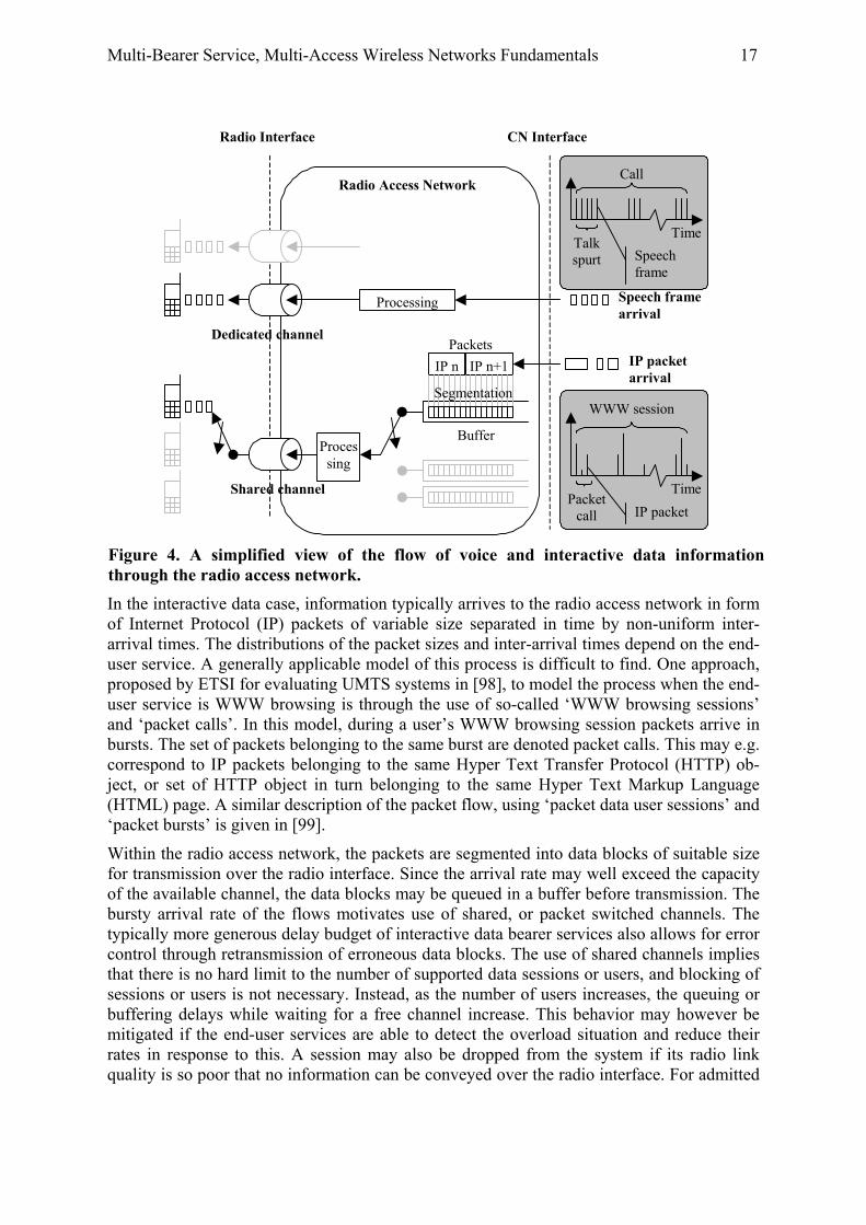
Multi-Bearer Service, Multi-Access Wireless Networks Fundamentals 17
In the interactive data case, information typically arrives to the radio access network in form of Internet Protocol (IP) packets of variable size separated in time by non-uniform inter-arrival times. The distributions of the packet sizes and inter-arrival times depend on the end-user service. A generally applicable model of this process is difficult to find. One approach, proposed by ETSI for evaluating UMTS systems in [98], to model the process when the end-user service is WWW browsing is through the use of so-called ‘WWW browsing sessions’ and ‘packet calls’. In this model, during a user’s WWW browsing session packets arrive in bursts. The set of packets belonging to the same burst are denoted packet calls. This may e.g. correspond to IP packets belonging to the same Hyper Text Transfer Protocol (HTTP) ob-ject, or set of HTTP object in turn belonging to the same Hyper Text Markup Language (HTML) page. A similar description of the packet flow, using ‘packet data user sessions’ and ‘packet bursts’ is given in [99].
Within the radio access network, the packets are segmented into data blocks of suitable size for transmission over the radio interface. Since the arrival rate may well exceed the capacity of the available channel, the data blocks may be queued in a buffer before transmission. The bursty arrival rate of the flows motivates use of shared, or packet switched channels. The typically more generous delay budget of interactive data bearer services also allows for error control through retransmission of erroneous data blocks. The use of shared channels implies that there is no hard limit to the number of supported data sessions or users, and blocking of sessions or users is not necessary. Instead, as the number of users increases, the queuing or buffering delays while waiting for a free channel increase. This behavior may however be mitigated if the end-user services are able to detect the overload situation and reduce their rates in response to this. A session may also be dropped from the system if its radio link quality is so poor that no information can be conveyed over the radio interface. For admitted
Radio Access Network
Buffer
Packets Dedicated channel
Shared channel
Radio Interface
Time Talk spurt
Call
Speech frame
Time Packet
call
WWW session
IP packet
IP n IP n+1
Segmentation
IP packet arrival
Speech frame arrival
CN Interface
Processing
Processing
Figure 4. A simplified view of the flow of voice and interactive data information through the radio access network.

18 Multi-Bearer Service, Multi-Access Wireless Networks Fundamentals
sessions an acceptable quality, measured e.g. in delay or data rate or a function thereof should be maintained. Again, the task of the radio access network may be summarized as to support as many sessions as possible while maintaining an acceptable delay or bitrate qual-ity.
2.4 Multi-Access Wireless Networks A multi-access network is in this dissertation defined as a network providing bearer services using at least two different radio access technologies, denoted sub-systems. It is further as-sumed that the sub-systems are run by a single operator or a set of cooperating operators. The coupling of the sub-systems may be done at different levels in the overall architecture. Figure 5 contains some examples applicable to IMT2000-like systems. These are intercon-nection through (i) a common BSC/RNC, (ii) a common Core Network, or (iii) a common node for Authorization, Authentication, and Accounting (AAA) functionality. Other inter-connection examples than those exemplified in Figure 5 also exist, e.g. using an interface between the BSCs of the different sub-systems or adding new dedicated interconnection nodes. Interconnection of IMT-2000 systems with non-IMT-2000 systems could also be done over the interfaces used in alternatives (i) – (iii).
What type of interconnection is preferred is a complex issue, and beyond the scope of this work. Typically, but not strictly necessarily, the closer to the radio interface the interconnec-tion is made, the more sophisticated traffic load sharing principles may be employed. Here it is simply assumed that the necessary input information for the principles proposed in Chapter 8 and Chapter 10 to work is available. This required information depends on the traffic load sharing principle used, but may include e.g. users’ bearer service type and radio resource cost, as well as system capacities and load levels per bearer service group.
(ii i)
M S
BS BS C/ R NC
Ra di o Acces s Network
C N g ateway
C N ed g e n o de
Inter- net
PS TN
BS BS C/ R NC
C N g ateway
C N ed g e n o de
Core Netwo rk
A A A
S ub-S ys tem 1
S ub-S ys tem 2Ra di o Acces s Network Core Netwo rk
(ii)(i)
Figure 5. Examples of multi-access system architecture using the IMT-2000 reference architecture: interconnection through (i) a common BSC/RNC, (ii) a common Core Net-work, or (iii) a common node for Authorization, Authentication, and Accounting (AAA).
19
Chapter 3 System Models and Performance Measures After an initial discussion of different modeling approaches, this chapter defines and dis-cusses the system models and performance measures used in the dissertation. A single access scenario is first covered, followed by a generalization for multi-access systems. The system models and performance measures are defined in as general ways as possible. This is done to make the general resource sharing and bearer service allocation principles as widely applica-ble as possible. In the case studies more precise models and performance measures are some-times necessary, such modifications are described in the corresponding chapters.
3.1 Performance Measuring and Modeling Approaches There are many ways to measure the performance of a wireless system. These alternatives also affect the models used for the performance evaluation. First, performance can be meas-ured from an end-user perspective as well as from an operator’s perspective. These are not contradictory, but the desired system characteristics differ. End-users are typically interested in their own Quality-of-Service (QoS), e.g. in terms of voice quality or bitrate, and the price they pay for it. A wide service area may also be of interest. An operator is presumably more interested in the revenue the system as a whole generates, as well as the costs associated with generating this revenue. Depending on what phase of its lifetime the system is in; different aspects may be identified as suitable performance measures. In a system just being deployed, if the traffic demand is distributed over a large area, increasing the coverage area is probably most important for increasing the revenue. In later stages, when sufficient coverage is reached, increased revenue may be generated by attracting new customers by offering an ex-tended set of bearer services. Further, in cases where the demand for bearer services is high, the revenue can be increased by improving the capacity of the system. All the above meas-ures may be used to determine the performance of wireless systems. In this dissertation an operator’s perspective is taken, and system capacity is used as the foremost performance measure. It is thus assumed that the systems studied have sufficient coverage and offer a suf-ficient set of bearer services.
Also capacity may be measured in several ways3. Within the telecommunication theory field, capacity C is often defined as the maximum service rate or maximum throughput S of a channel or a system [100]:
{ }SC max= (1)
No requirements on user-level quality Quser, such as delay, are included in these capacity measures. To take expected user-level quality into account, throughput-delay characteristics may be derived [101], and the maximum throughput for a certain required expected delay E[D] measured:
[ ]{ }max:max DDESC ≤= (2)
3 In this section some preliminary definitions of traffic load, quality, and capacity are made to describe alterna-tive approaches to measure performance. The definitions used in the thesis are given more precisely in the fol-lowing sections.

20 System Models and Performance Measures
In wireless systems, the quality may vary significantly between users, and some sort of fair-ness requirement is often introduced in the capacity measure. This may be accomplished by not only measuring the expected user quality E[Quser], but its full distribution. Capacity can then be defined e.g. as the maximum traffic load for which some minimum fraction of the users Qmin are satisfied, i.e. achieve acceptable quality [102]. The traffic load may be meas-ured in different units, e.g. in terms of number of users U or the aggregate number of bits generated by all users per unit time, i.e. the throughput S. The latter measure might be pre-ferred if the amount of data generated varies between users. Assuming that the number of users is used to represent the traffic load, the capacity is measured as:
{ }minmin ))((:max QQUQPUC useruser ≥<= (3)
In multi-bearer service scenarios measuring performance becomes yet more complex. The quality measures and traffic load measures typically differ between the bearer services. Us-ers and their bits associated with different bearer services may further be differently valued by the operator. Some different approaches to multi-bearer service capacity measuring are described below.
In the simplest case, users of different bearer services are treated equally. They are assumed to have the same quality requirements and the maximum total number of users, or their ag-gregate generated traffic, while this quality requirement is met is used as a capacity measure. In this case the multi-bearer service capacity is measured according to Equation (3). The use of a common quality requirement for all bearer services has the drawback that at the capacity limit some bearer services will have excessive quality, and/or some bearer services have too poor quality. Further, using only the total number of users as a traffic load measure is quite coarse, as the effort of supporting users and the revenue they generate typically varies with the bearer service type and the user’s subscription.
A more sophisticated approach is to use different quality measures Quser n and user and sys-tem quality requirements Quser n min and Qn min respectively for each bearer service n. Capacity may then be defined as the maximum traffic load for which all bearer services quality re-quirements are fulfilled.
{ }minmin ))((:max nnusernuser QQUQPUC ≥<= (4)
Such an approach is proposed by ETSI in their guidelines for evaluating UMTS radio access technologies [98], which also has been adopted by ITU [103]. In ETSI’s guidelines users of different bearer services have different requirements for being satisfied, and on the system-level capacity is defined as the highest traffic load for which at least a certain minimum frac-tion of users are satisfied for all bearer services. These fractions may be set to reflect the relative importance of different bearer services.
An alternative approach is to average the fraction of satisfied users over all bearer service types, and measure capacity as the traffic load where the average user satisfaction reaches a certain minimum value.
{ }min1 min )(:max QQQPUC N
n nusernusern ≥<= ∑ =α (5)
where αn is the fraction of users of bearer service n. This approach yields a simple one-dimensional quality requirement, but has the drawback that the fairness among bearer ser-vice groups is lost. It might well happen that all unsatisfied users are of the same bearer ser-

System Models and Performance Measures 21
vice type, for which the fraction of satisfied users may be far below the average for all bearer services.
In the ETSI guidelines the traffic load is measured as the aggregate number of bits per sec-ond generated by all users of the systems, regardless of bearer service. As discussed above this may be a somewhat blunt measure. For example, it is typically simpler to support a high throughput for bearer services with loose delay requirements than for bearer services with stringent delay requirements. To reflect this in the traffic load measure, the generated traffic could be measured per bearer service, e.g. using the number of users per bearer service Un, or the aggregate generated traffic could be measured together with a specific value of the bearer service mix {αn} used.
An additional approach to measure performance for multi-service networks is through the use of so-called utility functions [104]. This involves defining a utility function fn for each bearer service n, which maps some well-defined measure, e.g. the Signal to Interference Ra-tio (SIR) of the radio link, to a utility measure of each user. The utility measure may be re-garded as a soft satisfaction measure that is comparable across bearer service types. Users of multi-media bearer services may e.g. experience a higher utility than users of ordinary voice bearer services. The overall utility of the system, which may be used as a capacity measure, is then calculated as the sum of all users’ individual utilities, regardless of bearer service:
∑ = ==U
i iuserofservicenin SIRfC1
)( (6)
User fairness aspects may be taken into account through introducing negative utility values for users with poor quality, which reduces the capacity of an unfair system. The benefit of this approach is that a single scalar measure may be used to characterize the performance of the system. The drawback is loss of control of fairness among bearer services. It may also be difficult to define comparable utility functions for all bearer services. This is a difficult task already in the binary case when defining thresholds between satisfied and unsatisfied users.
In this dissertation performance measures close to those proposed by ETSI in [98] are used. Additionally, traffic load is measured with controlled mixes of bearer services. The motiva-tion for this selection is, apart from the ETSI recommendation, that they are relatively simple to use and provide control of the fairness among bearer service groups.
In what follows, the system models and performance measures used are defined and dis-cussed in greater detail. The models and performance measures are intended to apply for considering systems both in snapshots of time, as well as over a period of time. What differs between the snapshot and time dynamic approaches is the interpretation of certain random variables. These differences are highlighted when the random variables in question, repre-senting the number of offered users and experienced user quality, are introduced.
3.2 Traffic Load and Service Mix Generally a system with N bearer services is studied. The random variable Un denotes the number of bearer service n users per cell offered to the system. The expected number of of-fered users per cell E[Un] = un is used to measure the offered traffic load of bearer service n. In a snapshot analysis, Un varies between snapshots, whereas in a time-dynamic analysis Un varies over time. The expected total number of users per cell is:

22 System Models and Performance Measures
∑=
=N
nntot uu
1 (7)
A bearer service mix ,or shortly a service mix, is defined as a vector whose elements are the fractional contributions of each bearer service to the expected total number of users:
tot
NN u
uu ),,(),,( 11
KK
r == ααα (8)
Note that this is a many-to-one function, i.e. many sets of expected numbers of users result in the same service mix.
3.3 User and System-Level Quality The quality experienced by a user of bearer service n is measured by the real-valued scalar random variable Quser n. In a snapshot analysis Quser n represents an instant perceived quality, whereas in a time-dynamic analysis it is averaged per user. Examples of user-level quality measures include Frame Erasure Rate for voice bearer services, and bitrate and/or delay for data bearer services, more examples are provided in the case studies in Chapter 5 - Chapter 7. The cumulative distribution function )Pr()( qQqF nuserQ nuser
≤= depends on a complex va-riety of parameters, including e.g. traffic, mobility, and system characteristics. However, typically for a fixed set of other parameters, )(qF nuserQ increases with the expected number of users un of each bearer service n. A system level quality of bearer service n may be defined as a function g of the distribution of individual user quality:
))(( qFgQnuserQn = (9)
For example, assuming that users of bearer service n are satisfied if they experience a quality exceeding quser n min, then
)(1 minnuserQn qFQnuser
−= (10)
is the probability that a user of bearer service n in sub-system m is satisfied, i.e. roughly measuring the fraction of satisfied users. Further, in time-dynamic cases, if the system of random processes Quser n are stationary, Qn also represents the fraction of time a users is ex-pected to be satisfied.
3.4 Multi-Bearer Service Quality, Capacity and Capacity Regions To measure capacity in multi-bearer service systems a set of minimum system-level qualities Qn min for each bearer service n are selected. Then, for a certain set of traffic, mobility, and system assumptions etc., the per-bearer service capacity, or shortly the per-service capacity, of bearer service n is measured as the maximum expected number of users utot for which the system-level quality Qn exceeds Qn min. The per-service capacity typically depends on the service mix. Thus, for a given service mix αr the per-service capacity is defined as:
( ) ( ){ }min:max nntotn QQuC ≥= ααr (11)
Specifically the single-bearer service capacity of bearer service n is defined as:
)0,1( nkforCC knnnsingle ≠=== αα (12)

System Models and Performance Measures 23
Since utot = un/αn, it follows that Cn(αr ) is upper bounded by Csingle n/αn. The overall capacity C(αr ) is defined as the maximum aggregate traffic load for which all bearer services’ quality requirements are fulfilled:
( ){ }nQuQuC ntotntot ∀≥= min,:max)( αα rr (13)
According to the ETSI guidelines [98] the overall capacity is thus given by the smallest per-service capacity:
{ })(min)( αα rrnn CC = (14)
An example of how this capacity measure is used for a two-bearer service scenario is de-picted in Figure 6. By repeating this analysis for the range of all possible service mixes, a capacity region may be constructed. The capacity region is defined as:
( ){ }nQuQuu ntotnN ∀≥= min1 ,:),...,( αrK (15)
The capacity region hence is the set of expected number of users for which acceptable sys-tem-level quality is sustained for all bearer service types.
The above quantities are exemplified for a two-bearer service scenario in Figure 7 (left). A traffic load is given by the vector (u1, u2). A fixed service mix αr =(α1, α2), where α1+α2 =1, corresponds to traffic loads on a straight line from the origin with the angle arctan((1-α1)/α1) to the u1 axis. The per-service capacities Cn(αr ) each have endpoints at Csingle n on the un axis. The overall capacity limit C(αr ), is for each service mix given by the minimum per-service capacity. The capacity region K, delimited by C(αr ) thus equals the intersection of the areas delimited by the per-service capacities.
3.5 Normalized Measures When studying capacity in mixed bearer service systems, it is sometimes convenient to use normalized traffic measures. A normalized traffic load per bearer service is defined as:
nsingle
nn
Cul = (16)
Quality Q
Q1min
Traffic loadutot=u1+u2
Q2min
Q1(utot, αr )
Q2(utot, αr )
C2(αr )C1(αr )
C(αr ) = min {C1(αr ), C2(α
r )}
Figure 6. Example of quality versus traffic load behavior. The service mix αr is held constant.

24 System Models and Performance Measures
The aggregate normalized traffic load ltot is defined as the sum of the N different bearer ser-vices’ normalized loads:
∑ ==
N
n ntot ll1
(17)
A normalized service mix is defined as a vector whose elements are the fractional contribu-tions of each bearer service to the aggregate normalized traffic load:
tot
NN l
ll ),,(),,( 11
KK
r== λλλ (18)
The normalized per-service capacity of bearer service n, cn( λr
), is defined as:
( ) ( ){ }min:max nntotn QQlc ≥= λλr
(19)
Since ltot = ln/λn, it may be noted that cn( λr
) is upper bounded by 1/λn. The overall normal-ized capacity c is defined as:
( ) ( ){ } ( ){ }λλλrrr
nnnntot cnQQlc min:max min =∀≥= (20)
and may hence also be expressed as the smallest per-service capacity. The upper bound for c( λr
) is equal to the number of bearer services N. A normalized capacity region is defined as:
( ){ }nQlQll ntotnN ∀≥= min1 ,:),...,( λr
k (21)
The normalized quantities are exemplified for a two-bearer service scenario in Figure 7 (right). An interesting capacity reference in the normalized case is the capacity limit c( λ
r)
=1, which corresponds to a straight line between the endpoints ln=1. Similarly, necessary
C(αr ) = min{C1(α
r ), C2(αr )}
C2(αr )
u1
u2
Csingle 1
C1(αr )
(u1,u2)
ltot=1
c(λr
) = min(c1(λ
r), c2(λ
r))
c2(λr
)
l1
l2
1.0
1.0c1(λ
r)
(l1,l2)
Csingle 2
Arctan(u2/u1)= Arctan((1-α1)/α1)
Arctan(l2/l1)= Arctan((1-λ1)/λ1)
K k
Figure 7. Examples of the defined quantities for two bearer services. Left: absolute measures. Right: Normalized measures.
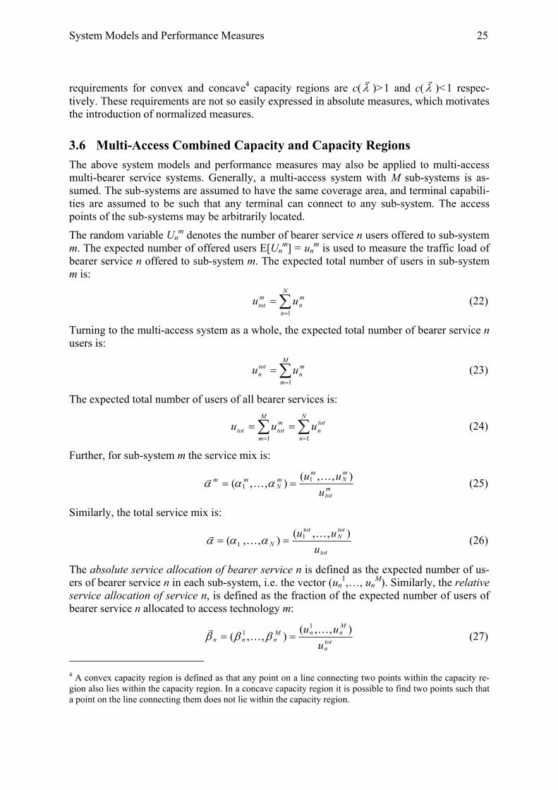
System Models and Performance Measures 25
requirements for convex and concave4 capacity regions are c( λr
)>1 and c( λr
)<1 respec-tively. These requirements are not so easily expressed in absolute measures, which motivates the introduction of normalized measures.
3.6 Multi-Access Combined Capacity and Capacity Regions The above system models and performance measures may also be applied to multi-access multi-bearer service systems. Generally, a multi-access system with M sub-systems is as-sumed. The sub-systems are assumed to have the same coverage area, and terminal capabili-ties are assumed to be such that any terminal can connect to any sub-system. The access points of the sub-systems may be arbitrarily located.
The random variable Unm denotes the number of bearer service n users offered to sub-system
m. The expected number of offered users E[Unm] = un
m is used to measure the traffic load of bearer service n offered to sub-system m. The expected total number of users in sub-system m is:
∑=
=N
n
mn
mtot uu
1 (22)
Turning to the multi-access system as a whole, the expected total number of bearer service n users is:
∑=
=M
m
mn
totn uu
1 (23)
The expected total number of users of all bearer services is:
∑∑==
==N
n
totn
M
m
mtottot uuu
11 (24)
Further, for sub-system m the service mix is:
mtot
mN
mmN
mm
uuu ),,(),,( 1
1K
Kr == ααα (25)
Similarly, the total service mix is:
tot
totN
tot
N uuu ),,(),,( 1
1K
Kr == ααα (26)
The absolute service allocation of bearer service n is defined as the expected number of us-ers of bearer service n in each sub-system, i.e. the vector (un
1,…, unM). Similarly, the relative
service allocation of service n, is defined as the fraction of the expected number of users of bearer service n allocated to access technology m:
totn
MnnM
nnn uuu ),,(),,(
11 KK
r== βββ (27)
4 A convex capacity region is defined as that any point on a line connecting two points within the capacity re-gion also lies within the capacity region. In a concave capacity region it is possible to find two points such that a point on the line connecting them does not lie within the capacity region.

26 System Models and Performance Measures
The relationship between the service mix and the relative service allocation is hence:
mmnn
mn βααβ = (28)
where βm = umtot / utot.
Similar to the single access case, the quality of bearer service n experienced by of a user in sub-system m is measured by the real-valued scalar random variable Quser
mn. A system level
quality of bearer service n in sub-system m may be defined as a function g of the distribution of individual user quality, i.e.
( ))(qFgQ mnuserQ
mn = (29)
Thus, similar to the single-access case, for a given service mix mαr the sub-system m capac-ity is defined as:
( ){ }nQuQuC nmm
totmn
mtot
mm ∀≥= min,:max)( αα rr (30)
Two alternative combined capacity definitions now exist. In the first, general case, for a given total service mix αr , the general combined capacity is defined as:
{ }mnnntotgeneral mm
nnmn
mQQuC,:min:max)(
∀=≥=
βααβαα rr (31)
where the expected quality Qn of bearer service n is given by:
∑=
⋅=M
m
mmn
mmultin
mnn uQQ
1),( αβ r (32)
Qnm
multi(utotm, mαr ) is defined as Qn
m(utotm, mαr ) in the single-access case, but may differ
somewhat due to trunking or diversity gain, see below. The second condition in Equation (31) is identical to Equation (28), i.e. simply the requirement that the sub-system user alloca-tions and service mixes results in the desired total service mix. Note that a degree of freedom here exists in how bearer services are allocated onto the sub-systems, and that the combined capacity hence depends on the bearer service allocation.
The general combined capacity region is in this case consequently the set of expected-number-of-users-vectors that can be accommodated by all sub-systems while maintaining acceptable quality for all bearer service types over all sub-systems.
{ }nQQuu nnNgeneral ∀≥= min1 :),...,(K (33)
The general combined capacity definition in Equation (31) allows system-level qualities Qnm
below the minimum requirement Qn min as long as the expectation over all sub-systems Qn exceeds Qn min. This poses a problem for users with terminals that are not capable of commu-nicating in all sub-systems. Such users may then experience a system level quality less than Qn min, and hence are less likely to be satisfied. To ensure that this does not happen, accept-able system-level quality must be required in all sub-systems. In this case the equal quality combined capacity is defined as:
{ }mnnmm
totm
multintotQequal mmnn
mn
mQuQuC ,:min),(:max)( ∀=≥= βααβααα rrr (34)

System Models and Performance Measures 27
The corresponding equal quality combined capacity region in this case is the set of expected-number-of-users-vectors that can be accommodated by all sub-systems while maintaining acceptable quality for all bearer service types in all sub-systems:
{ }mnQQuu nm
multinNQequal ,:),...,( min1 ∀≥=K (35)
Here, the latter equal quality capacity and capacity region definitions of Equations (34) and (35) are used, and henceforth for simplicity denoted only by the combined capacity C(αr ) and combined capacity region K. Appendix C discusses the applicability and implications on capacity of the different definitions. For large numbers of users the capacity difference is limited. Under certain assumptions the capacities will be equal as the expected number of users and the system bandwidth approach infinity.
The combined capacity may be expressed as the sum of the sub-system multi-access capaci-ties Cm
multi( mαr ):
mn
M
m
mmmulti
mmnn
mn
m
CC,:1
)()(∀==
∑=βααβα
ααr
rr (36)
The sub-system multi-access capacity definition is similar to the single-access case in Equa-tion (13):
( ){ }nQuQuC nmm
totm
multinmtot
mmmulti ∀≥= min,:max)( αα rr (37)
Noticeably however the sub-system capacity may differ between the multi-access and single-access cases, i.e. Cm
multi( mαr ) ≠ Cm( mαr ). This in turn depends on trunking or diversity gains in the multi-access case, due to which there exist user assignments such that Qn
mmulti(utot
m, mαr ) > Qn
m(utotm, mαr ), and as a result of this Cm
multi( mαr ) > Cm( mαr ). In blocking limited sys-tems, it is well known that larger resource pools yield reduced blocking and hence higher capacity per resource. Similar effects appear in interference limited systems, where a diver-sity gain is achieved from the reduced risk of outage in all sub-systems as compared to in a single sub-system. These effects may be dramatic for small expected number of users, but become less significant for large expected number of users. In this study, the latter case is targeted, and it is assumed that Cm
multi( mαr ) ≈ Cm( mαr ). Consequently, the combined capacity region is approximated by the sum of the sub-system single-access capacities:
mn
M
m
mm
mmnn
mn
m
CC,:1
)()(ˆ∀==
∑=βααβα
ααr
rr (38)
The accuracy of this approximation depends on the difference between Cmmulti( mαr ) and
Cm( mαr ). In Appendix B it is shown that under certain assumptions the approximation error asymptotically approaches zero as the expected number of users and the system bandwidth approach infinity. Some numerical examples of both blocking and interference limited sce-narios are also given.
Figure 8 depicts a simple example of an approximated combined capacity with two sub-systems supporting voice and data bearer services. Note that the combined capacity depends on the sub-system service allocation. This fact is utilized in Chapter 8 when maximizing the combined capacity.

28 System Models and Performance Measures
3.7 Valuing Bearer Services The above load and capacity measures do not reflect that bearer services may be valued dif-ferently. For example, supporting a certain number of voice users may produce higher reve-nue than supporting the same number of web browsing users. Assuming that the revenue generated by each bearer service may be expressed as a function vn(un), the total revenue generated by the system may be expressed as:
)(1 n
N
n ntot uvV ∑ == (39)
This measure allows comparison of revenues for different service mixes, which in turn may be used to try to control the service mix to increase revenue. This may in the short-term be done by an admission control scheme that targets the most profitable service mix, and in the long-term e.g. by marketing.
Noticeably, if all vn(un) are monotonically increasing functions, maximizing C(αr ) for a cer-tain service mix αr also maximizes Vtot for that service mix. Since at the capacity limit, un= αn·C(αr ), the total revenue is given by:
))((1
αα rCvV nN
n ntot ⋅= ∑ = (40)
In general, Vtot can be maximized jointly over αr and C(αr ). For a given service mix how-ever, the αns are fixed, and Vtot is maximized by maximizing C(αr ). With this as a motiva-tion the above revenue measure is not further used in this paper, but left as an item for fur-ther studies.
d1(v1)
(v, d)
voice
data
d2(v2)
Figure 8. The multi-access combined capacity is approximated with the sum of the sub-system capacities.

29
Chapter 4 Radio Resource Sharing in Multi-Bearer Service Interference Limited Wireless Networks
This chapter aims at deriving generally applicable resource sharing principles for interfer-ence-limited systems, and also at determining their expected performance. Using simple models, it is first shown that per-service capacity balancing can be used to maximize capac-ity in mixed bearer service systems fulfilling certain radio resource-related assumptions. Per-service capacity balancing is a slightly more general form of the QoS balancing proposed by Wang and Aghvami in [18] and [19]. Next it is shown that in interference limited systems per-service capacity balancing can be achieved by interference balancing, through which power is allocated to bearer service groups such that the maximum tolerable interference levels become equal for all bearer service groups. A simple theoretical analysis of the ex-pected multi-bearer service capacity of interference limited systems with and without inter-ference balancing is then provided. A set of scenarios with different interference tolerance characteristics is covered. Finally, some practical applications of the proposed principles are given.
Throughout this chapter rather simple models are used. Although some motivations for their validity are given when introducing them, the main motivation is provided in Chapter 5 - Chapter 7, where their validity is verified in a set of case studies.
4.1 Per-Service Capacity Balancing In this section it is shown that in systems for which radio resources may be described using a simple, scalar model, per-service capacity balancing may be used to maximize capacity. Be-fore proceeding with the analysis of per-service capacity balancing, the radio resource model used is presented.
4.1.1 A Simple Radio Resource Model
It is difficult to give a generally applicable radio resource model. In strictly channel limited systems, radio resources may be measured in terms of number of channels. A channel may in turn correspond to a frequency, time slot, spreading code, or a combination thereof. In strictly interference limited systems, the output power used to overcome the interference may be used as a radio resource measure. In general, systems are limited by a combination of lack of channels and interference, and the radio resource may be measured as a combination of number of channels and power.
In the analysis of per-service capacity balancing, it is simply assumed that the radio resource allocation to a bearer service can be seen as a parameter that can be used to control the per-service quality levels, and thereby also control the per-service capacities. Specifically it is assumed that:
(i) The amount of radio resource allocated to bearer service n may be measured as a real-valued scalar rn(αr ). If traffic load dependent radio resource allocation is used, rn(αr ) is the amount of resources allocated at the capacity limit.
(ii) The resource allocation of a bearer service decreases with the resource allocation for other bearer services, i.e.:

30 Radio Resource Sharing in Multi-Bearer Service Interference Limited Wireless Networks
knforrr
k
n ≠<∂∂ 0
)()(
ααr
r (41)
(iii) The per-service capacity Cn(αr , rn(αr )) increases with the resource allocation of the own bearer service, and hence because of Equation (41) decreases with the resource alloca-tion of other bearer services, i.e.:
≠<=>
∂∂
knkn
rrC
k
nn
;0;0
)())(,(
ααα
r
rr (42)
These assumptions are not generally applicable. Still, they may be motivated by that they appear to hold in some special cases. In strictly channel limited systems, if the number of channels allocated to a bearer service is increased, more users of that bearer service can be supported. Fewer channels would however remain for other bearer services, for which fewer users can be supported. Similarly, in a strictly interference limited system, if the power allo-cated to a bearer service is increased, more users of that bearer service could reach an ac-ceptable channel quality. However, the power allocated to some other bearer services de-creases, and fewer users of those bearer services would reach acceptable quality.
4.1.2 Per-Service Capacity Balancing Maximizes Capacity Per-service capacity balancing is characterized by that the per-service capacities for all bearer service are equal:
knCrCrC kknn ,)())(,())(,( ∀== ααααα rrrrr (43)
Under the assumptions of the previous section, it may be shown that per-service capacity balancing is a necessary and sufficient requirement for maximizing overall capacity. An ana-lytical proof for this is given in Appendix D. For a two-bearer service scenario a graphical proof is provided in Figure 9. This figure may also ease following the analytical and more general proof in Appendix D. As depicted in Figure 9, the more resources that are allocated to bearer service 1, the higher its per-service capacity. Further, since 0)(/)( 21 <∂∂ αα rr rr , this implies that less resources are allocated to bearer service 2, and the lower its per-service ca-pacity. The overall capacity C(αr ) is determined by the lowest per-service capacity
Capacity
C(αr , r1(αr )) =
min{C1(αr
, r1(αr )) , C2(α
r, r2(α
r ))}
Service 1 Resource usage
r1(αr
)
C1(αr
, r1(αr ))
C2(αr
, r2(αr )) Cmax(α
r )
Csingle 2/α2
Csingle 1/α1
Figure 9. Per-service capacity balancing maximizes capacity.

Radio Resource Sharing in Multi-Bearer Service Interference Limited Wireless Networks 31
min{Cn(αr ,rn(αr ))}. Hence, to improve overall capacity the lowest per-service capacity should be increased. Since the per-service capacities all grow with increased resource alloca-tion, this can be done by moving resources from the bearer services with excessive quality to the limiting bearer service, thereby improving its quality and increasing min{Cn(αr ,rn(αr ))}.
In the context of the illustration in Figure 6 in Section 3.4, per-service capacity balancing corresponds to moving the bearer service-2-quality-curve to the right at the expense of mov-ing the bearer service-1-quality-curve to the left. The effect of this is a gain in overall capac-ity as long as bearer service 1 does not become the limiting per-service capacity. The overall capacity is maximized when both bearer services reach their minimum quality levels for the same aggregate load.
Note that the per-service capacities depend on both the service mix and the resource alloca-tion. Different service mixes result in different resource allocations fulfilling Equation (43). Therefore, in dynamic scenarios where αr changes with time, these changes must be tracked by the resource sharing algorithm to maintain maximized capacity. Static resource sharing cannot maximize capacity in dynamic scenarios.
It should also be noted that per-service capacity balancing only maximizes capacity for a given set of Cn(αr , rn(αr )). Higher capacities can indeed be achieved if Cn(αr , rn(αr )) can be improved, e.g. by better RRM solutions within the bearer service groups, better receiver per-formance, etc. Such solutions are however outside the scope of this dissertation.
Equation (43) motivates the name per-service capacity balancing. Also note that since at the per-service capacity limit the quality of each bearer service just equals its minimum re-quirement. Thus, if Equation (43) holds, the following also holds:
)(,),( min αα rr CUnQUQ totntotn =∀= (44)
Above it was assumed that rn is a scalar. Similar examples also could be constructed when the resource is non-scalar, e.g. consists of a combination of power and number of channels etc. Then however, several balancing solutions may be found, which must be searched to find a global overall capacity maximum.
Reasoning similar to that given here is used by Wang and Aghvami when deriving their QoS-balancing power allocation scheme for CDMA-based systems in [18] and [19]. They observe that blocking for two bearer services can be traded against each other, and that ca-pacity reaches a maximum when blocking levels, which is the quality measure they consid-ered, are equal. Replacing blocking with the more general quality requirements, Qn min, in Equation (44), which need not be of the same form for different bearer services, the conclu-sion is the same as the one derived here. Further, it has also been proposed by Sampath et al. [8] that for a DS-CDMA uplink, at a capacity-wise optimal power allocation per user, all in-dividual QoS constraints are met with equality. This is similar to what is stated in Equation (44), although it deals with system-level qualities rather than individual QoS. This allows for more general definitions of quality and capacity, including measures such as fractions of sat-isfied users.
4.1.3 Resulting Capacity Regions The maximum overall capacity resulting from the above balancing procedure depends on the per-service capacity versus resource usage characteristics Cn(αr , rn(αr )) of the bearer ser-vices included. These in turn depend on what the limiting resource is, e.g. number of chan-nels, interference budget, or a combination thereof. The above relationships are typically

32 Radio Resource Sharing in Multi-Bearer Service Interference Limited Wireless Networks
quite complex, which prevents simple analysis. Below some very simplified cases are dis-cussed, from which interesting characteristics may however still be observed.
In addition to the assumptions in made in Section 4.1.1, in the below analysis it is assumed that the total radio resource is limited so that at the capacity limit ∑nrn( λ
r) = rtot. Further, the
normalized measures defined in Section 3.5 are used. The normalized per-service capacity cn( λ
r, rn( λ
r)) is lower bounded by 0 and upper bounded by 1/λn. If rn( λ
r) is a scalar, these
extremes occur at rn( λr
)=0 and rn( λr
)=rtot respectively. With normalized measures the con-dition for per-service capacity balancing from Equation (43) becomes:
kncrcrc kknn ,)())(,())(,( ∀== λλλλλrrrrr
(45)
With the above assumptions some basic characteristics of the achievable overall capacity may be simply derived:
a) If all normalized per-service capacities depend linearly on the resource usage, i.e.:
nrrrc
ntot
nnn ∀
⋅=
λλλλ )())(,(r
rr (46)
then with per-service capacity balancing, according to Equation (45):
knrr
rr
ktot
k
ntot
n ,)()(∀
⋅=
⋅ λλ
λλ
rr
(47)
this yields:
knrrk
knn ,)()( ∀
⋅=
λλλλr
r (48)
and further since ∑nrn( λr
) = rtot:
totk
kn
k
knn n rrrr ==
⋅= ∑∑ λ
λλ
λλλ )()()(rr
r (49)
Thus, for per-service capacity balancing the resource allocations rk =λk⋅ rtot for all k should be used. This results in the overall capacity (with per-service capacity balanc-ing):
λλ
λλλλλλ
rr
rrr∀=
⋅⋅
=⋅
== 1)())(,()(maxktot
totk
ktot
kkk r
rrrrcc (50)
A linear capacity region between the single-bearer service endpoints is thus achieved.
b) From the above analysis it may also be seen that if all normalized per-service capacities are smaller than linearly dependent on the resource usage, i.e.:
nrrrc
ntot
nnn ∀
⋅<
λλλλ )())(,(r
rr (51)
which occurs e.g. if d2cn( λr
,rn( λr
))/drn2( λr
) > 0 for all n, then cmax( λr
)<1, i.e. a concave capacity region is achieved.

Radio Resource Sharing in Multi-Bearer Service Interference Limited Wireless Networks 33
c) Similarly, if all normalized per-service capacities are larger than linearly dependent on the resource usage, i.e.
nrrrc
ntot
nnn ∀
⋅>
λλλλ )())(,(r
rr (52)
which occurs e.g. if d2cn( λr
,rn( λr
))/drn2( λr
) < 0 for all n, then cmax( λr
)>1, i.e. a convex capacity region is achieved.
Again, the resource is generally a combination of an amount of channels and their quality, and the above does not directly apply. However, in the extreme cases of pure blocking and interference limitation, some interesting observations may be made. In a strictly channel- or queuing-limited system with divided channel pools, the trunking efficiency causes the per-service capacities to be smaller than linearly dependent on resource usage, hence case b) ap-plies and cmax( λ
r)<1, i.e. a concave capacity region is achieved. In a strictly interference-
limited system on the other hand, if interference is bearer service independent, linearly grow-ing per-service capacities may arise, and hence case a) applies and cmax( λ
r)=1. The latter
case is discussed in detail in Section 4.3.1.
Note that the normalized capacity regions are just re-scaled version of the absolute ones. The above principles thus apply also to absolute capacity region shapes, although the absolute capacity Cmax(αr ) is not so simply expressed.
It should also be noted that the size of the aggregate resource may depend on the service mix, i.e. ∑nrn( λ
r) = rtot( λ
r). This may happen e.g. in an interference-limited system when the
maximum tolerable interference is service mix dependent. In such cases non-linear capacity regions arise. Further, also in cases where the limiting resource is not a scalar, e.g. in sys-tems limited by both interference and blocking, non-linear capacity regions appear.
4.2 Interference Balancing As discussed above, with the performance measures used, per-service capacity balancing is a necessary requirement for maximized capacity in operational scenarios for which the as-sumptions of Section 4.1.1 are valid. This section discusses how per-service capacity balanc-ing can be realized in interference-limited systems. The proposed interference balancing concept is applicable to both downlink and uplink, and regardless of multiple access tech-nology, FDMA, TDMA, CDMA etc., as long as the system is operating in interference lim-ited scenarios.
4.2.1 Interference Limited Operation To develop the interference balancing principle, some definitions and assumptions regarding interference characteristics are necessary. The interference caused by the users of bearer ser-vice n is measured by the random variable In. The distribution of this interference level de-pends on the total number of users in the system and the service mix. Its expectation5 E[In] is denoted in(utot, α
r ). In multiple bearer service scenarios, the aggregate expected interference is given by:
5 It should be noted that the interference levels in and itot may in principle be measured in arbitrary ways as long as they can be associated with the user and system-level qualities.

34 Radio Resource Sharing in Multi-Bearer Service Interference Limited Wireless Networks
∑ ==
N
n totntottot uiui1
),(),( αα rr (53)
The same expected aggregate interference itot is assumed to be experienced by all bearer ser-vices. For each αr , in(utot, α
r ) is assumed to be monotonically increasing with utot.
Under interference limited operation, as the name indicates, the interference level in the sys-tem determines the user-level quality and thereby also the system-level quality. Different sources of interference may further affect the quality differently, which introduces a depend-ency on the service mix. Thus, Quser n = f(itot, αr ), and Qn = g(itot, αr ), for some functions f and g. The function g is assumed to be decreasing, so that the minimum system level quali-ties Qn min can be associated with maximum interference levels imax n through:
),()( min1
max αα rrnn Qgi −= (54)
Under interference limited operation, the system capacity may hence be expressed as:
( ){ } niuiuC ntottottot ∀≤= )(,:max)( max ααα rrr (55)
In this dissertation, systems for which the above capacity definition is valid are defined as interference limited. By introducing the overall maximum interference level imax(αr ) = min{imax n(αr )} the capacity may be expressed as:
( ){ })(,:max)( max ααα rrr iuiuC tottottot ≤= (56)
Note that since in(utot, αr ) is monotonically increasing with utot, C(αr ) is monotonically in-
creasing with imax(αr ).
Illustrations of the above capacity measures are depicted in Figure 10 and Figure 11. Figure 10 shows examples of expected interference levels versus normalized traffic load ln = un/Csingle n behavior for two different bearer services. Here single-bearer service scenarios are assumed. The capacity Csingle n for each bearer service is limited by the maximum interfer-ence level imax n above which the quality for the bearer service falls below Qn min. A multiple bearer service scenario is depicted in the left graph in Figure 11. Now, the per-service capac-ity of bearer service n is reached when this aggregate interference itot reaches the maximum tolerable interference for bearer service n, i.e. for itot = imax n(αr ). The overall capacity C(αr )
0 20 40 60 80 100 1200
5
10
15
20
25
30
l1 = u1/Csingle 1 [%]
Inte
rfere
nce
i 1
imax1
0 20 40 60 80 100 1200
5
10
15
20
25
30
l2 = u2/Csingle 2 [%]
Inte
rfere
nce
i 2
imax2
Figure 10. Examples of single-bearer service interference in versus normalized traffic load ln behavior for two different bearer services.

Radio Resource Sharing in Multi-Bearer Service Interference Limited Wireless Networks 35
is limited by the smallest per-service capacity, and is thus reached when the aggregate inter-ference equals the minimum of the per-service maximum interference levels, i.e. for itot = min{imax n(αr )} = imax(αr ).
The shared resource rtot in interference limited scenarios is the common power budget Ptot used to overcome the interference to fulfill the signal-to-interference ratio required for ac-ceptable quality. The common power budget may be explicitly limited by a maximum output power of a common power amplifier, or implicitly by the aggregate generated interference reaching a maximum acceptable level. The resource allocation per bearer service corre-sponds to the part of the total power budget allocated to each bearer service, hence rn(αr ) = Pn(αr ). As before, if traffic load dependent power allocations is used, Pn(αr ) is the power allocated at the capacity limit. In what follows it is further assumed that:
(i) The power allocation of a bearer service decreases with the power allocation for other bearer services, i.e.:
knforPP
k
n ≠<∂∂ 0
)()(
ααr
r (57)
(ii) The maximum interference level per bearer service imax n(αr , Pn(αr )) increases with the power allocation of the own bearer service, and hence because of Equation (57) decreases with the resource allocation of other bearer services, i.e.:
≠<=>
∂∂
knkn
PPi
k
nn
;0;0
)())(,(max
ααα
r
rr (58)
Also note that the aggregate interference itot in the system is proportional to the total power budget Ptot. Simply increasing Ptot to increase imax(αr ) would thus not improve capacity since itot then would increase proportionally.
0 50 100 1500
5
10
15
20
25
ltot = U1/U1max + U2/U2max [%]
Inte
rfere
nce
i tot
imax(α ,P1)
imax(α ,P2)
c1(α ,P1)c2(α ,P2)
P1=Ptot-P2
imax1(αr
,P1) imax2(α
r,P2)
imax(αr ) imax(α
r,P1)
Interference
Figure 11. Left: Example of interference versus normalized traffic load behavior for two different bearer services in a mixed-bearer service scenario. Right: With interference balancing per-service power levels are adjusted so that maximum interference levels are equal.

36 Radio Resource Sharing in Multi-Bearer Service Interference Limited Wireless Networks
4.2.2 Interference Balancing Maximizes Capacity
In cases where the above assumptions are valid, it is possible to maximize imax(αr ) through selecting Pn(αr ) such that:
knPiPi kknn ,),(),( maxmax ∀= αα rr (59)
Further, since C(αr ) is strictly growing with imax(αr ), maximizing imax(αr ) also maximizes the overall capacity C(αr ).A proof of that this selection of Pn(αr ) maximizes capacity is given in Appendix D.
A graphical proof for a two-bearer service scenario is given in the right graph of Figure 11. The larger the fraction of the total power allocated to bearer service 1, the higher total inter-ference level it tolerates, i.e. the higher imax 1(αr ). However, this also results in less power allocated to bearer service 2, which then tolerates less interference. The smallest of the per-service interference tolerance levels, imax(αr ), is maximized when the per-service interfer-ence tolerance levels are equal. This also maximizes the overall capacity C(αr ) since it is strictly growing with imax(αr ).
In summary, with interference balancing capacity is maximized through adjusting per-service power levels so that all maximum interference levels are equal, hence the name inter-ference balancing.
4.2.3 Adjusting Power Levels Note that the per-service power levels correspond to the sum of the power levels of the indi-vidual users of the bearer service. Adjusting the group power level may hence be realized by many different user power level adjustments. For non-power controlled bearer services the fixed bearer power levels may e.g. be equally adjusted for all users. For power controlled bearer services such an approach would affect the SIR target, and hence the quality for all users. A better approach is to adjust the maximum power for each user, which only affects the ability to reach the SIR target.
The per-bearer service power levels that maximize capacity vary with the service mix. This is true even in cases where the maximum interference levels do not depend on the service mix, since the number of users in the bearer service group that share the power changes. An attractive property of adjusting the (maximum) power per bearer within the bearer service group is that it inherently takes this into account. The power level per bearer service group flexibly follows the number of users in the bearer service group, and hence also follows changes in the service mix. This would not be the case if fixed power budgets were statically allocated per bearer service class. Such a solution would have to be optimized for a single service mix, and deviations from the targeted service mix would render performance losses.
Fairness aspects of interference balancing among users with different coverage characteris-tics (indoor and outdoor users) have been investigated for DS-CDMA-based systems in [105]. As might be expected, it is seen that as long as the systems operate under interference limited conditions, fairness among indoor and outdoor users is maintained.
4.3 Expected Performance This section discusses what capacity regions may be expected depending on some different interference tolerance characteristics. A general expression for the capacity region is first

Radio Resource Sharing in Multi-Bearer Service Interference Limited Wireless Networks 37
presented. Specific results are then derived for a set of different assumptions of the interfer-ence characteristics.
The interference contribution of user k of bearer service n is denoted by the random variable Jkn with expectation E[Jkn] = jn(itot, α
r ). The interference caused by all users of bearer service n is thus given by:
∑ == nU
k knn JI1
(60)
The expected interference from bearer service group n is thus given by:
[ ] ),(),( αα rrtotnnntotn ijuIEii == (61)
Since the aggregate interference itot is the sum of the interference stemming from all bearer service groups, the relationship between the expected number of users per bearer service un and the expected aggregate interference level itot is given by:
∑∑ ==⋅==
N
n totnntotN
n ntot ijuiii11
),(),( αα rr (62)
The capacity is for each service mix αr limited by the maximum tolerable interference. Thus, for any αr , C(αr )=∑nun(αr ) is given by un(αr ) such that:
{ })(min)()()( maxmax1αααα rrrr
nN
n nn iiju ==⋅∑ = (63)
This equation also forms the capacity region limit. The shape of the capacity region hence depends on the interference contribution per user in and the maximum sustainable total inter-ference level imax. In what follows, three scenarios with different assumptions on the above quantities are further analyzed:
1) Both the maximum tolerable interference level and the interference contribution per user are independent of the service mix.
2) The maximum tolerable interference level depends on the service mix, whereas the in-terference contribution per user is independent of the service mix.
3) Both the maximum tolerable interference level and the interference contribution per user depend on the service mix.
The applicability of these scenarios is discussed in Section 4.4. Note that scenarios 2 and 3 may also be used to model blocking limitation and effects of higher order statistics of the interference.
4.3.1 Maximum Interference and Interference Contribution Independent of Service Mix
In this basic scenario it is first assumed (Assumption 1) that the expected interference contri-bution per user for a given total interference level is independent of the service mix. For an arbitrary aggregate interference level Itot, the expected interference generated by a user of bearer service n is given by:
)1,(
)(=
=ntotn
tottotn
iuiijα
(64)
where un(itot,αn=1) is the single-bearer service relationship between traffic load and interfer-ence.

38 Radio Resource Sharing in Multi-Bearer Service Interference Limited Wireless Networks
The expected number of users for any αr for a fixed aggregate interference level itot then fol-lows the simple relationship:
∑∑ == ==⋅=
N
nntotn
totn
N
n totnntot iuiuijui
11 )1,()()()(
ααα rr (65)
Simplifying this yields:
1)1,(
)(1
==∑ =
N
nntotn
n
iuu
ααr (66)
In the two-bearer service scenario this becomes:
1)1,(
)()1,(
)(22
2
11
1 ==
+= α
ααα
tottot iuu
iuu rr
(67)
This is an intercept form of the straight-line equation connecting the single-bearer service end-points u1(itot,α1=1) and u2(itot,α2=1). Thus, for any fixed aggregate interference level, the number of users that can be supported follows a straight-line relationship. Note that this holds regardless of the shape of the single-bearer service interference-to-traffic-load relation-ships. Figure 12 depicts the number of sustainable users of the bearer services exemplified in Figure 10 for some different aggregate interference levels.
To estimate the capacity region it is further assumed (Assumption 2) that the maximum tol-erable interference levels imax n are independent of αr , i.e. imax n(αr ) = imax n and imax(αr ) = imax. Inserting imax(αr ) = imax in Equations (63) and (64) yields:
max1max
max1 max )1,(
)()()( iiu
iuiju N
nnn
nN
n nn ==
=⋅ ∑∑ == ααα rr (68)
Dividing by imax yields:
1)1,(
)(1
max=
=∑ =
N
nnn
n
iuu
ααr (69)
Figure 12. An example of aggregate interference versus normalized traffic load behav-ior. For any fixed aggregate interference level (including the maximum levels) a linear relationship between the number of sustainable users is achieved.

Radio Resource Sharing in Multi-Bearer Service Interference Limited Wireless Networks 39
For a two-bearer service system the capacity region limit becomes:
1)1,(
)()1,(
)(2max2
2
1max1
1 ==
+= α
ααα
iuu
iuu rr
(70)
In the example in Figure 12, the solution to the above equation is plotted in bold and pro-jected on the traffic load plane.
With interference balancing, characterized by imax 1 = imax 2 = imax, a capacity region delimited by a straight line between the single-bearer service capacities Csingle 1 and Csingle 2 is achieved:
1)()(2
2
1
1 =+singlesingle C
uCu αα rr
(71)
This further corresponds to an overall normalized capacity c(αr ) = 1 for arbitrary service mixes αr , which may also be referred to as preserved relative capacities. Such a case is shown in Figure 13 (left), where it is seen that balancing the maximum interference levels of the two bearer services (here realized by lowering P1 and thereby imax1 so that imax1 = imax2) yields a straight-line capacity limit region between the single-bearer service capacity end-points.
4.3.1.1 Non-Balanced Performance
Equal maximum interference levels may not always be achieved. The relative loss in capac-ity for a bearer service m with unbalanced maximum interference levels is given by:
{ }
msingle
mnmmsinglem C
iuCloss
)1,(min max =−=
α (72)
The larger the difference in maximum interference, the larger the loss. However, also the characteristics of the relationship between the traffic load and interference between imax m and min{imax n} affects the loss. If the number of additional users managed for the above interfer-ence increase is comparatively small, also the loss in capacity will be small, and vice-versa. The other way around, it is better for a bearer service that tolerates a high interference to have a steep interference versus traffic load behavior than a flat one close to the capacity limit. This phenomenon is depicted in Figure 13 (right), where it is seen that when the inter-
Figure 13. Two examples of aggregate interference versus normalized traffic load be-havior. Capacity limits, given by the projections on the x-y plane, are maximized when the maximum interference levels are equal. Imbalances yield smaller losses for steeper interference vs. traffic load behaviors (left).
Imbal-ance loss
Imbal-ance loss

40 Radio Resource Sharing in Multi-Bearer Service Interference Limited Wireless Networks
ference-to-load behavior of the interference-excessive bearer service 1 is linear (less steep than in the original case), the losses in the unbalanced case are larger.
4.3.2 Maximum Interference depends on Service Mix In this scenario assumption 2 is relaxed, i.e. the maximum tolerable interference does depend on the service mix, i.e. imax = imax(αr ). At the capacity limit the interference contribution per user is now given by:
)1),((
)())((max
maxmax
==
nnn iu
iijαα
αα r
rr (73)
Inserting this in the expression for the capacity region limit, i.e. Equation (63), yields:
)(
)1),(()()(
))(()(
max1max
max
max1
ααα
αα
αα
rr
rr
rr
iiu
iu
iju
N
nnn
n
N
n nn
==
⋅
=⋅
∑
∑
=
=
(74)
Dividing by imax(αr ) yields:
1)1),((
)(1
max=
=∑ =
N
nnn
n
iuu
αααr
r (75)
For a two-bearer service system the capacity region limit is thus given by:
1)1),((
)()1),((
)(2max2
2
1max1
1 ==
+= αα
ααα
αr
r
r
r
iuu
iuu (76)
This is similar to the previous scenario. The difference is that the maximum interference level now depends on the service mix αr , i.e. on the relationship between u1 and u2. Using graphical reasoning, for each service mix αr , the capacity region limit is given by the inter-section of the straight-line between u1(imax(αr ),α1=1) and u2(imax(αr ),α2=1) and the straight-line corresponding to the service mix in question. Noticeably, if the maximum interference imax(αr ) = min{imax n(αr )} is larger than the maximum single-bearer service interference lev-els imax n(αn=1) for all n, a normalized capacity c(αr ) > 1 is achieved. Similarly, if the maxi-mum interference level is smaller than the single-bearer service maximum interference levels for all bearer services, a normalized capacity c(αr ) < 1 is achieved. In more general cases where imax(αr ) < imax n(αn=1) for some n and imax(αr ) > imax n(αn=1) for other n, whether c(αr ) > 1 or < 1 also depends on the number of users versus interference characteristics un(i,αn), and simple rules are more difficult to find. The third example below illustrates this.
Three examples are depicted in Figure 14. In all examples it is assumed that the maximum interference levels per bearer service depend linearly on the service mix according to:
[ ]dBii nnnnn )-(1)( 0max αγα −= (77)
The interference tolerance is thus reduced from its single-bearer service scenario level i0n by up to γn dB when the fraction of other-bearer service users increases. In the first example (top plots) γn is set to +2dB for both bearer services (n=1, 2), in the second example (middle plots) γn is set to -2dB for both bearer services, and in the third example γ1 = +1dB and γ2 = -3dB is assumed. The single-bearer service interference levels i01 and i02 are assumed to be equal in the first two examples, but differ in the third example. The left plots show the result-
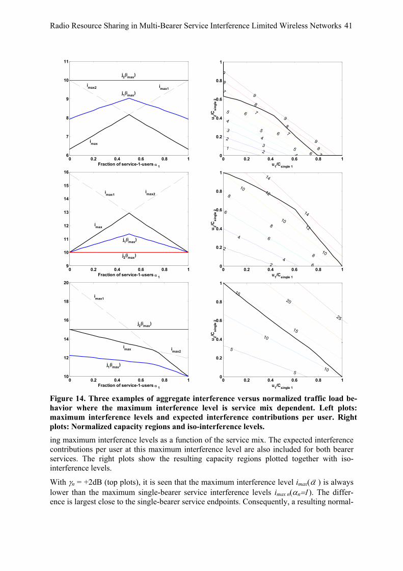
Radio Resource Sharing in Multi-Bearer Service Interference Limited Wireless Networks 41
ing maximum interference levels as a function of the service mix. The expected interference contributions per user at this maximum interference level are also included for both bearer services. The right plots show the resulting capacity regions plotted together with iso-interference levels.
With γn = +2dB (top plots), it is seen that the maximum interference level imax(αr ) is always lower than the maximum single-bearer service interference levels imax n(αn=1). The differ-ence is largest close to the single-bearer service endpoints. Consequently, a resulting normal-
0 0.2 0.4 0.6 0.8 16
7
8
9
10
11
Fraction of service-1-users α 1
imax
imax1 imax2
j2(imax)
j1(imax)
0 0.2 0.4 0.6 0.8 10
0.2
0.4
0.6
0.8
1
u1/Csingle 1
u 2/Csi
ngle
2
12
23
3
4
4
4
5
5
5
6
6
6
7
7
7
7
8
8
8
8
9
9
9
9
0 0.2 0.4 0.6 0.8 19
10
11
12
13
14
15
16
Fraction of service-1-users α 1
imax
imax1imax2
j1(imax)
j2(imax)
0 0.2 0.4 0.6 0.8 10
0.2
0.4
0.6
0.8
1
u1/Csingle 1
u 2/Csi
ngle
2
2
2
4
4
6
6
6
8
8
8
10
10
10
12
12
14
14
0 0.2 0.4 0.6 0.8 110
12
14
16
18
20
Fraction of service-1-users α 1
imax
imax1
imax2
j1(imax)
j2(imax)
0 0.2 0.4 0.6 0.8 10
0.2
0.4
0.6
0.8
1
u1/Csingle 1
u 2/Csi
ngle
2
5
5
10
10
15
15
2
20
25
Figure 14. Three examples of aggregate interference versus normalized traffic load be-havior where the maximum interference level is service mix dependent. Left plots: maximum interference levels and expected interference contributions per user. Right plots: Normalized capacity regions and iso-interference levels.

42 Radio Resource Sharing in Multi-Bearer Service Interference Limited Wireless Networks
ized capacity c(αr ) < 1 is achieved. With γn = -2dB (middle plots) on the other hand, the maximum interference level is always larger than the maximum single-bearer service inter-ference levels, and a normalized capacity c(αr ) > 1 is achieved.
In the third case with γ1 = +1dB and γ2 = -3dB, imax(αr ) < imax 1(α1=1), but imax(α ) > imax 2(α2=1). Despite the fact that imax(αr ) < imax 1(α1=1), a normalized capacity c(αr ) > 1 is achieved. This depends on that the normalized loss in bearer service-1 users due to the lower interference level is compensated for by a normalized increase in servcice-2 users, for which the maximum interference level has increased. This behavior typically appears when γ1 + γ2 > 0, and slightly dependent on un(i) for the two bearer services.
4.3.2.1 Balanced Performance
Also with varying maximum interference tolerance levels interference balancing may be used to maximize capacity. It cannot be achieved by merely balancing the maximum single-bearer service interference levels however, since the maximum tolerable interference level now varies with the service mix. Instead, to achieve interference balancing the power budg-ets per bearer service have to be adjusted adaptively for each service mix. This could be done in several ways. One alternative is to adapt the power budget for bearer service 2 so that its maximum interference level equals the maximum interference level for bearer service 1. Assuming that the interference tolerance grows linearly with the power budget allocated to a bearer service, this may be done by multiplying the power budget for bearer service 2 by a factor ∆P2(αr ) given by6:
)()()( 2max1max2 ααα rrr iiP =∆ (78)
Other power reallocations that balance maximum interference levels also exist, e.g. such that imax(αr ) becomes constant. Noticeably, as is later seen in Equation (86), these all result in the same capacity region, only the operating interference levels differ.
As a result of this the maximum interference levels are balanced:
)()()()()( max1max2max22max ααααα rrrrr iiiPi bal ==⋅∆= (79)
Adjusting the power budget for bearer service 2 with the factor ∆P2(αr ) causes the interfer-ence level for a fixed expected number of users to increase with the same factor ∆P2(αr ):
),()(),( 22222 ααα rrr uiPui bal ⋅∆= (80)
This also means that for a fixed expected number of users, the interference contribution per user is adjusted with a factor ∆P2(αr ):
),()(),( 22222 ααα rrr ujPuj bal ⋅∆= (81)
A fixed expected number of users however corresponds to different interference levels in the balanced and unbalanced cases.
)),(/(),( 222 ααα rrr Piuiu tottotbal ∆= (82)
Combining Equations (81) and (82), the relationship between the interference contributions per user for a fixed interference level becomes: 6 In practical cases with limited power budgets it may not be possible to increase the power budget for a ser-vice, instead the power budgets for other services must be decreased.

Radio Resource Sharing in Multi-Bearer Service Interference Limited Wireless Networks 43
)),(/()(),( 2222 αααα rrrr PijPij tottotbal ∆⋅∆= (83)
Inserting this Equation (73) yields:
)1)),(/(())(
)1)),(/(()(/)()())((
22max
max
22max
2max2max2
=∆
==∆
∆⋅∆=
αααα
ααααααα
rr
r
rr
rrrr
Piui
PiuPiPij
n
n (84)
The capacity region thus becomes limited by:
1)1),(/)((
)()1),((
)(22max2
2
1max1
1 ==∆
+= ααα
ααα
αrr
r
r
r
Piuu
iuu (85)
Using Equation (79) this may also be rewritten as:
1)1),((
)()1),((
)(22max2
2
11max1
1 ==
+= αα
ααα
αr
r
r
r
iuu
iuu (86)
Note that this expression only depends on the original (before balancing) maximum interfer-ence levels per bearer service, and not on how the interference balancing is achieved. Using graphical reasoning, for each service mix αr , the capacity region limit is given by the inter-section of the straight-line between u1(imax 1(αr ),α1=1) and u2(imax 2(αr ),α2=1) and the straight-line corresponding to the service mix in question. This is similar to the unbalanced case, but with the maximum overall interference imax(αr ) replaced by the per-bearer service maximum interference in the single-bearer service scenario. Note that if imax n(αr ) grows with αn for at least one n, and is constant for other n, a convex capacity region is achieved. In the opposite case a concave capacity region is achieved.
Figure 15 shows the same examples as the first two in Figure 14, but with interference bal-ancing according to Equation (78). The maximum interference levels are now all equal to the maximum interference levels for bearer service 1 in the unbalanced case. With γn = +2dB (top plots), it is seen that the interference contribution per bearer service 1 user grows slower with the fraction of bearer service-1-users, than does the maximum interference level. Thus, the smaller the fraction of bearer service 1-users, the larger fraction of the interference budget each of them consume. The same is true for bearer service 2-users, for which the in-terference contribution falls faster with increasing fractions of bearer service 2-users than does the maximum interference level. The relative resource consumption is hence smallest close to the single-bearer service endpoints, and larger with a mix of users. This explains the concave shape of the capacity region in the top right plot.
With γn = -2dB (lower plots) on the contrary, the interference contribution per bearer service n-user decreases in relation to the maximum interference level when the fraction of bearer service n-users increases. The relative resource consumption per user is smaller for a mix of bearer services than close to the single-bearer service endpoints. This motivates the convex shape of the lower right capacity region.
4.3.3 Maximum Interference and Interference Contribution Depends on Service Mix
In this scenario it is assumed that not only the maximum interference tolerance, but also the interference contribution per user varies with the service mix, i.e. jn=jn(itot, α
r ).

44 Radio Resource Sharing in Multi-Bearer Service Interference Limited Wireless Networks
Without further assumptions on how the interference contribution depends on the service mix, it is not possible to derive a more precise capacity region expression than given in Equation (63). One possible such assumption is that, for a two-bearer service system, the in-terference from bearer service 1 to bearer service 2 is scaled up a factor γ1, and the interfer-ence from bearer service 2 to bearer service 1 is scaled up a factor γ2. The equivalent inter-ference level experienced by bearer services 1 and 2 are thus:
21122211 ; iiiiii eqtoteqtot +=+= γγ (87)
The interference contribution per user may then be given by
)1,(),( n === αα neqtottotntotn iijij r (88)
Which for the two different bearer services yields:
)1,(
),(;)1,(
),(22112
2112
12211
2211
=++
==+
+=
αγγα
αγγα
iiuiiij
iiuiiij tottot
rr (89)
The capacity region is hence delimited by:
0 0.2 0.4 0.6 0.8 16
8
10
12
14
16
Fraction of service-1-users α 1
imax1=imax2=imax
j1(imax)
j2(imax)
0 0.2 0.4 0.6 0.8 10
0.2
0.4
0.6
0.8
1
u1/Csingle 1
u 2/Csi
ngle
2
1 2
2
3
3
4
4
4
5
5
5
6
6
6
7
7
7
8
8
8
9
9
9
0 0.2 0.4 0.6 0.8 16
8
10
12
14
16
Fraction of service-1-users α 1
imax1=imax2=imax
j1(imax)
j2(imax)
0 0.2 0.4 0.6 0.8 10
0.2
0.4
0.6
0.8
1
u1/Csingle 1
u 2/Csi
ngle
2
2
24
4
6
6
6
8
8
8
10
10
10
12
12
12
14
14
14
Figure 15. The first two examples of Figure 14 but with interference balancing. If lower other-bearer service interference than own-bearer service interference is tolerated, a concave capacity region is achieved (top plots). If on the other a hand a higher other-bearer service interference than own-bearer service interference is tolerated, a convex capacity region is achieved (lower plots).

Radio Resource Sharing in Multi-Bearer Service Interference Limited Wireless Networks 45
)()1,(
))(()1,(
))((max21
22112
2112
12211
2211 ααγ
γααγγα r
rriii
iiuiiu
iiuiiu
=+==+
++
=++ (90)
Interference balancing may as in the previous section be done according to Equation (78). The relationship between the interference contribution per user in the balanced and unbal-anced case is further given by Equation (83). In this case this yields:
)1),(/)((
)1),(/)(()(/)()(
)),(/()(),(
222112
211
222112
22112
2222
=∆++
=
==∆+
∆+⋅∆=
=∆⋅∆=
ααγγ
ααγαγα
αααα
r
r
rr
rrrr
Piiuii
PiiuPiiP
PijPij tottotbal
(91)
The capacity region is hence limited by:
)()1),(/)((
))(()1,(
))((max21
222112
2112
12211
2211 αααγ
γααγγα r
r
rriii
Piiuiiu
iiuiiu
=+==∆+
++
=++ (92)
Repeating the example from the previous section, with interference balancing, yields the re-sults shown in Figure 16. The capacity regions are similar to the ones with service mix-independent interference contributions. The interference contribution dependency on the ser-vice mix though does emphasize the non-linear characteristics of the capacity regions some-what. Intuitively, in the convex case, this is due to that when more interference is tolerated; the interference contribution per user is also lower for a given interference level, and vice-versa in the concave case.
4.4 Applicability of the Results The applicability of the presented principles and results depends on the validity of the as-sumptions made. This is discussed below. The applicability of the principles to WCDMA
0 0.2 0.4 0.6 0.8 10
0.2
0.4
0.6
0.8
1
u1/Csingle 1
u 2/Csi
ngle
2
1 2
2
3
3
4
4
4
5
5
5
6
6
6
7
7
7
8
8
8
9
9
9
0 0.2 0.4 0.6 0.8 10
0.2
0.4
0.6
0.8
1
u1/Csingle 1
u 2/Csi
ngle
2
2
2 4
4
6
66
8
8
8
10
10
10
12
12
12
14
14
14
Figure 16. Examples of aggregate interference versus normalized traffic load behavior where the maximum interference level and interference contributions per user are ser-vice mix-dependent. The non-linear characteristics of the capacity regions are now somewhat more emphasized.

46 Radio Resource Sharing in Multi-Bearer Service Interference Limited Wireless Networks
and GSM/EDGE-based systems, and their ability to explain the resulting capacity regions is verified in Chapter 5 - Chapter 7.
4.4.1 Interference Limited Operation Interference-limited operation is assumed. This is typically true for DS-CDMA-based and tight frequency reuse GSM/EDGE-based systems. For clusters of Wireless LANs this should also be valid. Blocking limitation may further to some extent be taken into account, see dis-cussion on assumption 2 below.
The definition of interference limited operation used in this study is that the interference level in the system determines the system quality. Other terms are sometimes used to de-scribe this condition, e.g. power limited operation.
4.4.2 Interference Contribution dependency on Service Mix Assumption 1 states that the interference contribution per user depends only on total system interference, and not on the service mix. This should be valid if interference stemming from different bearer services is equally damaging, i.e. when the carrier-to-interference ratio re-quired for acceptable quality does not depend on the source of interference, but only on its average level. If on the other hand higher order statistics of the interference differ signifi-cantly between bearer services, e.g. due to different on-off patterns, the assumption may not be valid. In such cases, an interference contribution per user that varies with the service mix may be expected. This is modeled as described in Section 4.3.3, where assumption 1 is as-sumed not to be valid.
Interference averaging techniques, such as random frequency hopping or DS-CDMA, effi-ciently reduces the effects of different interference patterns. In this case each link experi-ences an average of a set of interference patterns from other links. The larger the set, the less visible the characteristics of individual patterns. For GERAN-based systems employing ran-dom frequency hopping, the averaging set size corresponds to the number of frequencies hopped over. For DS-CDMA-based systems the set size corresponds to the number of users sharing the carrier, and hence decreases with increased bitrates. In summary, assumption 1 should apply to GSM/EDGE-based systems with random frequency hopping over a reason-able number of frequencies7, and for DS-CDMA-based systems with moderate bitrates.
4.4.3 Maximum Interference dependency on Service Mix Assumption 2 states that the maximum tolerable interference is independent of the service mix. As assumption 1, this is expected to be valid if interference stemming from different bearer services is equally damaging. The applicability should thus be as above. Some excep-tions exist though.
If the power available to overcome the interference varies with the service mix, the maxi-mum tolerable interference levels will also depend on the service mix. Such a power alloca-tion principle is used e.g. in WCDMA/HS-DSCH. Here, voice users are first allocated the power required to reach their SIR target from a common power budget; the remaining power is then allocated to the HS-DSCH. Hence, the more voice users, the less likely that they can all fulfill their targets. Further, also the less power is left for user of the HS-DSCH. See fur-ther Chapter 7. 7 Note that the power back-off possibly used for EDGE in 8PSK mode indeed affects the interference contribu-tion. However, this is not dependent on the service mix, and thus does not violate assumption 1.

Radio Resource Sharing in Multi-Bearer Service Interference Limited Wireless Networks 47
Service mix-dependent interference tolerance may also be used to extend the scope of the presented analysis to model effects of blocking limitation. For service mixes for which blocking occurs for a bearer service, the maximum interference level for that bearer service may be reduced to reflect the reduction in served traffic. This typically yields convex capac-ity regions. Intuitively this may be explained by the existence of a ‘free interference budget’ left by a partially blocking limited bearer service at its capacity limit.
4.4.4 Non-Balanced Operation
Interference balancing may not always be used. This may for example be due to coverage problems involved with reducing the power levels for some bearer services in order to bal-ance their maximum interference levels with those of other bearer services. The complexity of a service mix-dependent interference balancing scheme may also prevent use of interfer-ence balancing in cases where the maximum interference depends on the service mix.
4.4.5 Adaptive End-User Services In the derivation of the per-service capacity balancing principles, it is assumed that each bearer service has a minimum quality requirement Qn min, which in turn may be defined e.g. as the fraction of satisfied users. For adaptive end-user services, e.g. Adaptive Multi Rate (AMR) voice, also using adaptive multi-modal bearer services, it is not obvious how to apply this. At least two alternatives exist. Firstly, the adaptive bearer services supporting the adap-tive end-user services could be regarded as one bearer service like all others, and users are satisfied if their quality exceeds a certain threshold in one of the modes of the adaptive bearer service. Secondly, the modes of the adaptive bearer service could be treated as indi-vidual bearer services, each having their own definition of satisfied users. Changing modes in the adaptive end-user service and adaptive bearer service would then also result in a change in service mix.
4.4.6 Time-Scale Applicability Throughout this chapter, dynamics in radio and traffic conditions are largely neglected. The interference contribution per users is e.g. always represented by its expected value i. Conse-quently the derived principles and results may be expected to apply only on a long-term time perspective. Taking radio and traffic dynamics into account better capacity figures than those derived in this paper may be achievable.
4.5 Summary Per-service capacity balancing can be used to maximize capacity in multiple bearer service cellular systems for which radio resources may be modeled in a simple, scalar way. In inter-ference-limited scenarios this can be accomplished by interference balancing. Interference balancing can further be realized by adjusting the maximum output power per individual bearer for each bearer service. This solution has the benefit of not statically allocating a fixed power budget per bearer service group, which might render performance losses, but instead flexibly follows variations in the service mix.
If the maximum tolerable interference level and the interference contributions per user are independent of the service mix, linear capacity regions arise. This case is the one most often seen in previous multi-bearer service studies, e.g. for the DS-CDMA uplink [7] - [19]. Under these conditions, interference balancing results in a capacity region delimited by a straight-line between the single-bearer service capacity endpoints. Hence, the single-bearer service

48 Radio Resource Sharing in Multi-Bearer Service Interference Limited Wireless Networks
capacities are preserved in a relative sense. If interference balancing cannot be achieved, the loss in capacity is given by the traffic load loss associated with the difference in maximum interference levels between the bearer services. This loss is typically lower for power-controlled bearer services.
If the interference tolerance depends on the service mix, service mix-dependent interference balancing is required to maximize capacity. The resulting performance depends on whether the tolerable interference levels from other bearer services are higher or lower than the toler-able own-interference. The former case results in convex capacity regions, whereas the latter case yields concave capacity regions. One example of the former case is a system where one bearer service is partially blocking limited.
In the former case, where the maximum tolerable interference level and the interference con-tributions per user are independent of the bearer service mix, the proposed theory may be used to predict multi-bearer service capacity regions based on single-bearer service interfer-ence to traffic load characteristics. In the latter case, where the maximum tolerable interfer-ence level or the interference contributions depend on the service mix, these dependencies need to known to predict the capacity regions. Finding these dependencies may in some cases involve actually evaluating the capacity for mixed bearer services, and thereby directly achieving the capacity regions. In such cases the theory is hence limited to explaining rather than predicting the shape of the capacity regions.

49
Chapter 5 Multi-Bearer Service Case 1 – Voice and WWW in GSM/EDGE
In this chapter the interference balancing principles developed in Chapter 4 are applied to a mixed voice and WWW GSM/EDGE system. A short GSM/EDGE overview is first pro-vided. It is then shown how interference balancing can be realized in GSM/EDGE systems through service-based power setting. Next, the models and assumptions used in this case study are described. This is followed by a presentation of numerical results for a set of dif-ferent scenarios. Simulated performance with and without interference balancing is com-pared mutually, as well as to the theoretically expected performance of Section 4.3.
5.1 GSM/EDGE Overview This section gives an overview of the GSM/EDGE Radio Access Network (GERAN). Some fundamental architecture and service aspects are first presented. This is followed by a brief look at how different bearer services may be realized using the GERAN radio protocol stack. Finally, some details are given on the key-elements of the EDGE concept; 8-PSK modula-tion and Link Quality Control. More comprehensive descriptions of GSM in general and GERAN are available in [106] and [107] respectively.
5.1.1 System Architecture and Service Aspects Figure 17 depicts the role of GERAN in the overall UMTS and GSM system architecture (as of 3GPP release 5). As UTRAN, GERAN uses the Iu interface to connect to the UMTS Core Network (CN). It connects to the packet and circuit switched domains of the UMTS core network (3G SGSN & 3G MSC) through the Iu-ps and Iu-cs interfaces respectively. For com-patibility with pre-3G Mobiles Stations (MSs), the A and Gb interfaces towards the standard GSM and GPRS core networks (MSC & SGSN) are kept. GERAN and UTRAN uses differ-ent radio interfaces towards the Mobile Stations. The WCDMA radio interface of UTRAN is denoted Uu, whereas the GERAN radio interface is denoted Um. A more detailed system ar-chitecture description is available in the GERAN overall description from 3GPP [107].
The use of the UMTS core network implies that bearer service management and negotiation from an application perspective is identical for GERAN and UTRAN. Thus, as with
Iu-ps
M S U u
UTRAN
RAN CN edge node
SGSN
3G M SC Iu-cs
G b
M SC A
3G SGSN
M S U m
GERAN
Figure 17. GERAN parallels UTRAN within UMTS system architecture. The approach is to offer a common set of bearer services but in different frequency bands.

50 Multi-Bearer Service Case 1 – Voice and WWW in GSM/EDGE
UTRAN, GERAN provides the core network with Radio Access Bearer (RAB) services. The RABs are divided into four different QoS classes; conversational, streaming, interactive, and background. The different types of RABs are further characterized with a number of attrib-utes, e.g. guaranteed bitrate, maximum delay and bit error rate. The principle idea is that ar-bitrary bearer services should be possible to specify using these attributes, and offered by the RAN. The UMTS and IMT2000 QoS concepts are further described in [4] and [5] respec-tively.
Within the GERAN the RABs are further mapped to one or several Radio Bearers. The radio bearers are realized by parameter settings of the radio interface protocols in the GERAN and MS. Depending on the QoS requirements of the associated RAB, different parameter settings of the radio interface protocols are used. This is further discussed in the next section.
The system and service architecture approach may be summarized as for UTRAN and GERAN to offer a common set of bearer services, but operate in different frequency bands. UTRAN should be used in UMTS frequency bands whereas GERAN should be used in GSM frequency bands.
5.1.2 User Plane Protocols and Bearer Realization To support the large variety of radio access bearers in a flexible and efficient way, different modes of the radio-specific protocols Packet Data Convergence Protocol (PDCP), Radio Link Control (RLC) and Medium Access Control (MAC), are used. By combining these modes with a set of physical layer parameters several radio bearers can be realized. [107]
The user plane protocol structure for GERAN is depicted in Figure 18. The same PDCP as for UTRAN is used to offer bearers to the Core Network (CN) in the same way as for UMTS. PDCP contains header compression functionality. The RLC protocol provides seg-mentation and re-assembly in the unacknowledged mode, extended by ARQ functionality including incremental redundancy in the acknowledged mode. The MAC protocol enables multiple users and flows to share a common transmission medium. Shared or dedicated channels may be allocated depending on which type of multiplexing is desired. Transparent modes of each protocol enable minimized overhead in case the functionality is not required. The physical layer supports different types of logical channels, characterized by different modulation formats (8PSK or GMSK), channel coding (punctured convolutional codes), and interleaving depths. Examples of such logical channels are different dedicated-type Traffic Channels (TCH) and shared-type Packet Data Traffic Channels (PDTCH), each associated with a set of coding schemes, interleaving depths and modulation formats. The GERAN
Non-transparent Transparent
Acknowledged Unacknowledged
Dedicated
PDCP
RLC
TCH, PDTCH etc.
MACShared
Transparent
Phy Figure 18. Simplified GERAN radio interface user plane protocol architecture. Differ-ent protocol modes are combined to realize different radio bearers.

Multi-Bearer Service Case 1 – Voice and WWW in GSM/EDGE 51
overall description from 3GPP [107] provides a more detailed description of the different protocol layers and their modes, as well as list of references to detailed specifications for each layer. Brief examples of how the protocol modes can be combined to create different bearers are given below.
5.1.2.1 Conversational
A general conversational bearer can be accommodated e.g. by using either the transparent or the non-transparent PDCP mode, the unacknowledged RLC mode, and a suitable MAC mode. PDCP performs IP/UDP/RTP header compression. The unacknowledged RLC mode segments PDCP frames, numbers RLC blocks to detect lost blocks, and selects appropriate coding schemes.
Different bitrates may be achieved by selecting modulation and coding schemes and allocat-ing multiple slots. Target bit error rates may be achieved by selecting modulation and coding schemes in combination with applying power control. Tailored voice solutions would typi-cally use the transparent PDCP and RLC modes together with the dedicated MAC mode and TCH logical channels to reduce overhead. End-to-end Voice over IP bearers are enabled by the non-transparent PDCP mode.
5.1.2.2 Streaming
Streaming bearers with relatively strict delay requirements may be built and maintained in the same way as conversational bearers. However, if the delay requirements are slightly higher compared to conversational bearers, streaming bearers may use increased interleaving depths to enhance the performance. For streaming bearers with looser delay requirements, a more efficient approach may be to base streaming bearers on the acknowledged RLC mode, using the delay budget for retransmissions. The acknowledged RLC mode typically achieves a desired bitrate at lower radio qualities than unacknowledged mode, and thereby may in-crease capacity.
5.1.2.3 Interactive and Background
Interactive and background bearers are typically built using the ‘non-transparent’ PDCP and RLC modes, together with the shared MAC mode and PDTCH logical channels. A central part of these bearers, referred to as EGPRS bearers, is Link Quality Control, see further Sec-tion 5.1.4.
5.1.3 The EDGE Physical Layer – 8PSK Enables Higher Peak Data Rates For compatibility and co-existence with GSM, EDGE has many physical layer parameters in common with GSM. This includes 200 kHz channel spacing, 8 timeslots per TDMA frame and 4.615 ms TDMA frame duration. In order to achieve higher data rates, EDGE introduces the new modulation scheme linear 8PSK. Together with the symbol rate of 271 ksymbols/s this facilitates a maximum gross data rate of 554 kbps/carrier, which is three times higher than for standard GSM. The standard GMSK modulation of GSM may still be used in situa-tions where a more robust modulation is needed. The 8PSK modulation is continuously 3π/8 phase shifted. This decreases the peak to average ratio, but also enables the receiver to dis-tinguish between 8PSK and GMSK modulated training sequences, thus allowing blind detec-tion of modulation. The selection of 8PSK for EDGE in favor of e.g. QAM-based modula-tion schemes was based on its relatively low peak-to-average power ratio, together with its ability to fit in the same spectrum mask as GMSK. A more detailed description of the EDGE physical layer is available in the standard, see [108] and [109].

52 Multi-Bearer Service Case 1 – Voice and WWW in GSM/EDGE
5.1.4 The EGPRS Link Layer – LQC Utilizes Varying Link Quality A characteristic of cellular systems is the varying link quality within a cell. This is especially true for GERAN, which compared to other 3G technologies has rather limited means to measure and compensate for these variations by power control. Typically, different modula-tion and coding schemes are optimal for different link qualities. This can be utilized by dy-namically adapting the modulation and code rate with respect to the current link quality – which is also referred to as Link Quality Control.
EGPRS employs a combined link quality control scheme with both Link Adaptation (LA) and Incremental Redundancy (IR) (or Hybrid Type II/III ARQ). In short, the Modulation and Coding Scheme (MCS) for initial block transmissions may be selected based on link quality measurements. If retransmissions are needed the robustness is increased through joint decod-ing of all transmission attempts. In terms of maximizing throughput an efficient and simple solution is to employ pure IR, i.e. using an initial code rate of 1 (equivalently uncoded). This approach efficiently utilizes peaks in the link quality through the high bitrates achieved when the first transmission attempt is successful. However, in situations with very poor link qual-ity, pure IR may lead to quite large numbers of retransmissions required for each block, which in turn may result in long block delays or protocol stalling. To mitigate these effects the number of retransmissions required may be limited by using an initial code rate lower than 1.
Bitrate versus channel quality performance for the cases of pure IR and pure LA, i.e. with no joint subblock decoding are depicted in Figure 19. Ideal LA operation is assumed, i.e. for each link quality the modulation and coding scheme maximizing the bitrate is selected. De-spite this, the pure IR, using only MCS9, provides bitrates exceeding those of LA over the full range of studied link qualities. In more realistic scenarios without access to perfect link quality information, the LA performance decreases due to sub-optimal selection of modula-tion and coding schemes. The IR performance is in the other hand not affected by this since it does not rely on link quality measurements. Thus, in realistic scenarios a larger difference between the two schemes than indicated by Figure 19 may be expected. Intuitively the lim-ited means of GERAN to measure and control the radio link quality is compensated for by the independence of such measures of IR.
A more detailed description of the link quality control scheme is provided in [82]. In the standards link quality control details are described within the RLC/MAC and channel coding specifications, see [110] and [108] respectively.
Regarding other link layer aspects, as for standard GPRS, selective repeat ARQ is used. However, to improve protocol performance the window size is increased for EGPRS. This reduces the risk of protocol stalling, but may also increase delay. Additionally, support for segmenting and compressing ACK/NACK bitmaps is introduced to further avoid protocol stalling. Also the Medium Access Control (MAC) functionality is similar to that of standard GPRS, supporting both shared and dedicated channels. [110]
The overhead introduced by the RLC and MAC layers reduce the peak bitrate of the RLC layer to 59.2kbps per timeslot. At the maximum all 8 timeslots on a carrier can be allocated to one mobile station, hence yielding a peak bitrate of 8 × 59.2 = 473.6kbps.
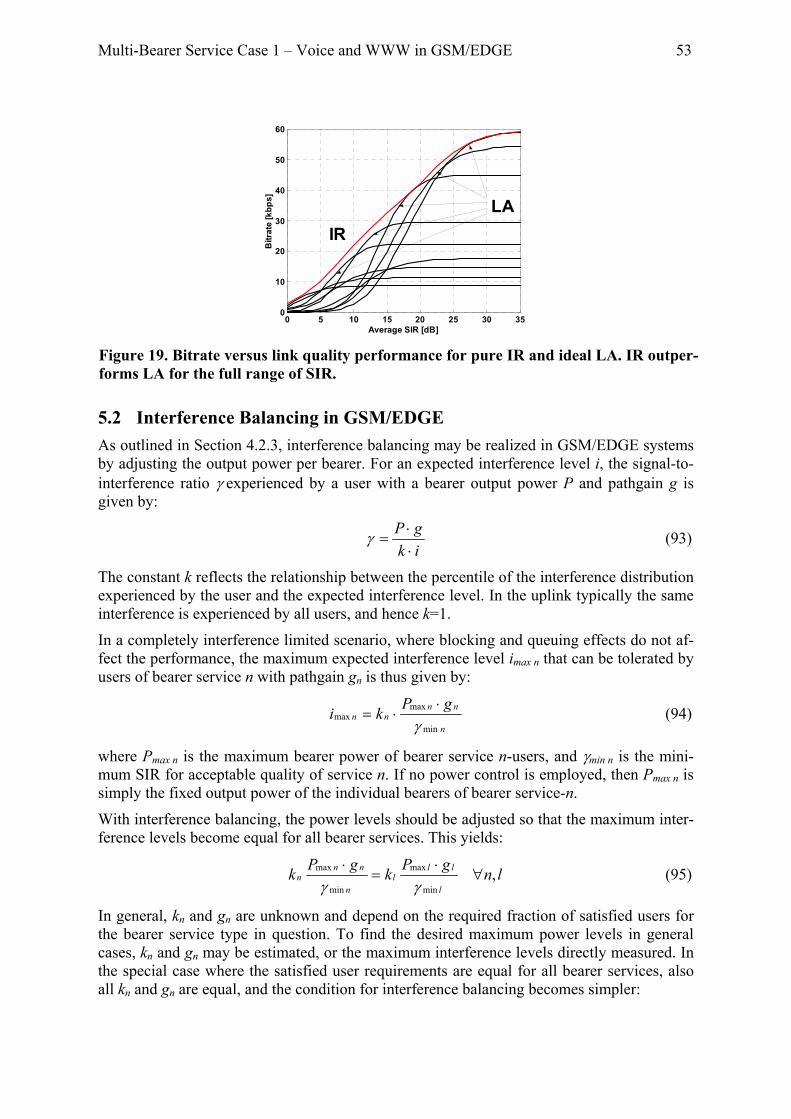
Multi-Bearer Service Case 1 – Voice and WWW in GSM/EDGE 53
5.2 Interference Balancing in GSM/EDGE As outlined in Section 4.2.3, interference balancing may be realized in GSM/EDGE systems by adjusting the output power per bearer. For an expected interference level i, the signal-to-interference ratio γ experienced by a user with a bearer output power P and pathgain g is given by:
ikgP
⋅⋅
=γ (93)
The constant k reflects the relationship between the percentile of the interference distribution experienced by the user and the expected interference level. In the uplink typically the same interference is experienced by all users, and hence k=1.
In a completely interference limited scenario, where blocking and queuing effects do not af-fect the performance, the maximum expected interference level imax n that can be tolerated by users of bearer service n with pathgain gn is thus given by:
n
nnnn
gPkimin
maxmax
γ⋅
⋅= (94)
where Pmax n is the maximum bearer power of bearer service n-users, and γmin n is the mini-mum SIR for acceptable quality of service n. If no power control is employed, then Pmax n is simply the fixed output power of the individual bearers of bearer service-n.
With interference balancing, the power levels should be adjusted so that the maximum inter-ference levels become equal for all bearer services. This yields:
lngPkgPkl
lll
n
nnn ,
min
max
min
max ∀⋅
=⋅
γγ (95)
In general, kn and gn are unknown and depend on the required fraction of satisfied users for the bearer service type in question. To find the desired maximum power levels in general cases, kn and gn may be estimated, or the maximum interference levels directly measured. In the special case where the satisfied user requirements are equal for all bearer services, also all kn and gn are equal, and the condition for interference balancing becomes simpler:
0 5 10 15 20 25 30 350
10
20
30
40
50
60
Average SIR [dB]
Bitr
ate
[kbp
s]
IR LA
Figure 19. Bitrate versus link quality performance for pure IR and ideal LA. IR outper-forms LA for the full range of SIR.

54 Multi-Bearer Service Case 1 – Voice and WWW in GSM/EDGE
lnPPl
l
n
n ,min
max
min
max ∀=γγ
(96)
The maximum bearer power is thus set proportional to the minimum SIR requirement.
Figure 20 shows bearer quality8 versus link quality for the GERAN Multi-Rate 5.9kbps (MR59) and Enhanced Full Rate (EFR) voice bearers as well as for the EGPRS interactive data bearer. This plot together with QoS requirements for the different bearers can be used to estimate the power offset. As an example, assume that the voice bearer requirement is 1% Frame Erasure Rate (FER) with EFR, and that the interactive data bearer requirement is 10kbps per timeslot. According to Figure 20 the voice requirement is reached at approxi-mately 8dB SIR, and the interactive data requirement at 5dB SIR (disregarding queuing ef-fects). Consequently, the power for the interactive data bearer should be set 8 – 5 = 3dB lower than for the voice bearer to maximize capacity. If different fractions of satisfied users are desired, e.g. 90% for interactive data and 95% for voice, this needs to be compensated for. The required compensation can be estimated from typical or expected interference dis-tributions. In the system studied here the difference between the 10th and 5th percentile of SIR is roughly about 3dB. Taking this into account in the above example the interactive data power should be decreased another 3dB resulting in a total power offset of 3 + 3 = 6dB. Power offsets for other bearer services may be derived in similar ways.
5.3 Models, Assumptions and Analysis Technique This section presents the user behavior, radio network, and GERAN system models used for evaluating the performance of the GERAN concept. The user behavior and radio network models used here are similar to those recommended by 3GPP and ITU and in [98] and [103], but differ somewhat in parameter settings. Due to the relatively complex nature of the stud-ied system, the performance analyses are done using stochastic simulations. This section also provides a description of the dynamic multiple-cell system simulator employed. A summary of models used and simulation parameters is listed in Table 1 in the end of this section.
8 Various protocol effects (ranging from RLC to TCP) make the bitrate experienced by the user less than indi-cated in this plot. To get closer to user perceivable performance a mapping from radio bearer performance tak-ing the above aspects into account is required.
0 4 8 1210
-3
10-2
10-1
100
Average SIR [dB]
Fram
e Er
asur
e R
ate
0 4 8 120
10
20
30
Bitr
ate
per T
imes
lot [
kbps
]EFR
MR59
EGPRS
Figure 20. Bearer quality versus average SIR for interactive data and voice bearers.

Multi-Bearer Service Case 1 – Voice and WWW in GSM/EDGE 55
5.3.1 User Behavior Modeling Two types of users are studied: web browsing (denoted WWW) and voice. Measurement-based WWW [111] and voice [112] traffic models are used to generate packets and talk-spurts for users in the system. Short descriptions of these follow.
WWW users enter the system and start their sessions according to a Poisson process. In the simulations, the arrival rate of this process is varied for studying different system loads. The average session length is 100s. Within a session a user requests a number of HTTP objects. The inter-arrival time between HTTP objects is modeled with a four-state hyper-exponential distribution with a mean of 11s. HTML pages consisting of multiple HTTP object are mod-eled by a state with short inter-arrival times. The size of the HTTP objects is log-normally distributed with a mean of 8.8kbyte, and a standard deviation of 44kbyte. The HTTP objects are segmented into Transmission Control Protocol (TCP) frames of maximum size 1460 bytes, which in turn are encapsulated in IP packets of maximum size 1500 bytes. To model a varying packet delay of the Internet, the inter-arrival time between IP packets belonging to the same HTTP object is exponentially distributed with a mean of 0.1s. During a session the average offered load from one user is 6.4kbps. The WWW model is based on measurements of traffic over telephone line modems, which have data rates similar to those expected for GERAN bearers. Thus, disregarding possible differences in charging, this model should bet-ter reflect the expected traffic than models based on measurements on faster Local Area Networks. Capacity evaluations with a set of alternative WWW traffic models, including the model used here, are performed in [84] and [86]. The results indicate that the resulting ca-pacity figures do not significantly depend on the traffic model used. A small dependency on the expected HTTP object size is seen though, exemplified e.g. by an 8% capacity loss for a HTTP object size reduction of 50%.
Also voice users enter the system and place calls according to a Poisson process, the inten-sity of which is varied to simulate different system loads. The call duration is exponentially distributed with a mean value of 90s (in the simulations this is limited to 15s to reduce simu-lation times). During a call, talk-spurts and silence periods are generated according to two different three-state hyper-exponential distributions. The average lengths of talk-spurts and silence periods are 1.1s and 0.7s respectively, yielding a voice activity factor of 60%.
Spatially, voice and data users are independently of each other and uniformly distributed over the system area. Further, users are exclusively either voice or WWW users, not both.
5.3.2 Radio Network Modeling
The radio network is modeled as a number of 3-sector cells placed on a regular grid, forming a hexagonal cell plan. An example of this is depicted in Figure 21 (left). Note that although a regular grid is used, the cell borders, plotted in the right part of Figure 21, are far from hex-agonal due to the shadow fading. The cell radius is 1km. The default cell/sector frequency reuse pattern9 is 1/3. In some evaluations a 1/1 reuse is used, and then explicitly stated.
Radio propagation is modeled with exponential path-loss and log-normally distributed shadow fading. To model an urban or sub-urban environment, a path-loss exponent of 3.5 and log-normal fading with standard deviation 8dB and correlation distance of 110m are as-sumed. Multi-path fading is modeled with a GSM Typical Urban (TU) channel profile [109] 9 For example, in a 1/1 reuse each frequency is repeated in every sector, and in a 4/12 reuse each frequency repeated in every 4th 3-sector cell.

56 Multi-Bearer Service Case 1 – Voice and WWW in GSM/EDGE
and a mobile speed of 3km/h. The output power is set sufficiently high (20W) to avoid cov-erage problems, rendering the radio link quality in the system limited by interference rather than noise.
Ideal frequency hopping over uncorrelated frequencies is assumed. The hopping patterns are pseudo-random between co-channel cells, which in addition to frequency diversity achieves interference diversity.
5.3.3 GERAN System Modeling As other cellular systems GERAN is a quite a complex system. To include all features and restrictions of the system in a radio network evaluation is not feasible. This section presents included as well as some excluded system specific aspects.
First of all, the evaluations cover only the GERAN user plane. Control signaling, e.g. in terms of spectrum required for broadcast channels or delays for setting up bearers, is not covered in the analyses, and not taken into account in the performance evaluation. For the user plane, the protocol modes used to realize the voice and interactive data bearers are de-picted in Figure 22. The modeling of each layer is also indicated. The protocol stack of GERAN release 5 is used to depict the bearer realization; however, similar bearers could also be realized using the GERAN release 99 protocol stack. The results presented in this work thus represent both the release 99 and release 5 standard.
Voice bearers are assumed to be realized using transparent PDCP, transparent RLC, and dedicated MAC. The functionality of these protocol modes is limited to delivering incoming Service Data Units (SDUs) to their peer entities, no overhead is added. Modeling of these layers is simply done through passing incoming speech frames directly to the physical layer. The physical layer for voice uses a full-rate Traffic Channel (TCH/F) [107]. Discontinuous Transmission (DTX) is used, i.e. the transmitter is switched off between talk spurts to reduce interference. For both voice and interactive data bearers the pulse shapes, modulation meth-ods, channel coding, and interleaving schemes of the physical layer are all directly imple-mented as specified in the GERAN standard in the link layer simulator, see Section 5.3.5.
Interactive data bearers are assumed to be realized using non-transparent PDCP, acknowl-edged RLC, shared MAC, and full-rate Packet Data Traffic Channels (PDTCH/F) on the physical layer. The MAC layer, which determines when users get to transmit and using which resources, is rather simply modeled. New packet flows entering the system are allo-
1 2 3
4 5 6
7 8 9
10 11 12
13 14 15
16 17 18
19 20 21
22 23 24
25 26 27
4
11 12
15
24
25 26
5
14
23
Figure 21. Example of hexagonal cell plan with uniformly distributed users (left), and coverage areas of three selected cells. Notice the irregular coverage areas.

Multi-Bearer Service Case 1 – Voice and WWW in GSM/EDGE 57
cated the channel in the cell with the least number of other flows allocated to it. This is done to get an even time-slot load. A random selection is made between equally loaded timeslots. Flows allocated to the same timeslot are scheduled in a Round Robin fashion, transmitting one 20ms radio block at a time. Voice bearers have strict priority over data bearers when al-locating channels. Thus, data bearers may be dynamically allocated on timeslots not occu-pied by voice calls, but are moved when the timeslot is requested by a voice call. However, data bearers are not allocated timeslots of ongoing voice calls that are temporary unused in between talk-spurts. Such a solution would indeed improve performance in channel limited scenarios, but does not improve performance in interference limited scenarios, see further [97]. Multi-slot operation is explicitly included in the system model. Also the selective ARQ mechanism of the RLC layer is explicitly modeled. A roundtrip time of 80ms, which might be expected when the ARQ functionality is located in the base station, and a polling interval of 5 RLC data blocks (corresponding to 100ms in the single-slot case) are assumed. An erro-neous RLC data block is thus retransmitted between 100ms and 180ms after the previous transmission. The ARQ window is assumed to be infinite, and there is no maximum number of retransmissions. This means that in principle there is no upper bound on the RLC data block delay.
The RLC model also contains the two Link Quality Control techniques link adaptation and incremental redundancy. In this case study pure incremental redundancy is employed, i.e. only MCS9 is used. All radio blocks are thus initially transmitted using rate-1 coded 8PSK, if decoding fails, another such block is transmitted and jointly decoded with the first, yield-ing an effective half-rate code. This procedure is repeated until the block is successfully de-coded.
PDCP functionality and overhead is not included in the analyses. Functionality-wise this means that TCP/IP headers are not compressed. This does not affect the results much though, since the TCP/IP header is regarded as payload information when calculating the Circuit Switched Equivalent bitrate. In terms of overhead, the PDCP header of 0-3 bytes, depending on PDCP mode, added to every IP packet is not included. This is regarded as a minor inaccu-racy since the IP packets are up to 1500 bytes long.
Algorithm-wise the system is rather simple. For data bearers fixed output power levels are used. For voice bearers power control is used in some scenarios. The intention of this is to verify that interference balancing works for a combination of power controlled and non-power controlled bearers. A partly SIR compensating scheme similar to the one of [113] with a SIR target of 10dB and an update interval of 120ms is used. Cell selection and hand-over is done randomly between the set of cells within 3dB of the strongest candidate. Drop-ping of interactive data users is done using a leaky-bucket scheme. A counter for each link is
Non-transparentTransparent
Dedicated
PDCP
RLC
MAC
Transparent
Phy PDTCH/F
Acknowledged
Shared
Voice Interactive data
TCH/F
Not modeled
Modeled
Modeled
Modeled
Modeled
Modeled
ARQ&LQC Modeled
Modeled Figure 22. Protocol modes assumed for the voice and interactive data bearers. The modeling of each layer is also indicated.
58 Multi-Bearer Service Case 1 – Voice and WWW in GSM/EDGE
initialized to its maximum value of 128. The counter is then decreased by 1 for every erro-neously transferred RLC block and increased by 10 for every successful block transmission. The counter is truncated at its maximum value of 128. Users whose counters reach zero are dropped. No dropping of voice users is employed.
5.3.4 Performance Measures The capacity of the systems in this case study is measured according to the general approach defined in Chapter 3. The specific quality and traffic load measures used are defined in this section.
5.3.4.1 User- and System-Level Quality for Voice
For voice bearer services, user-level quality is often measured in terms of Frame Erasure Rates (FER). A frame erasure is defined as an error in the most valuable so-called class 1a bits of the speech frame [108]. Various subjective Mean Opinion Score (MOS) tests have been done to investigate what FER figures yield acceptable voice quality for delays expected in typical GSM networks, see e.g. [85] and [114]. For the most common voice bearer, the 12.2kbps Enhanced Full Rate (EFR), FER requirements of 0.5-2% for acceptable voice qual-ity is often assumed. For another increasingly popular voice bearer, the Multi Rate 5.9kbps (MR59) within the Adaptive Multi Rate (AMR) family, a FER of 0.6% is required for voice quality comparable with that of EFR at 1% FER [85].
Reflecting this, the quality experienced by voice users is represented by the average FER, which is here defined as the average of the Frame Erasure Probability (FEP) over all Nframes frames of the user’s call:
frames
N
ivoiceuser NFEPQ
frames
∑=
=1
(97)
Based on the above studies, radio interface average FER requirements of quser voice max = 1% for EFR and quser voice max = 0.6% for MR59 bearers are used. Voice users are assumed to be satisfied if they experience acceptable FER, and they are not blocked. The system-level qual-ity Qvoice is measured as the fraction of satisfied users. For a system in which over a certain period of time Ncalls calls have been attempted, of which NFER had unacceptable FER, and Nblocked were blocked, this is defined as:
callsblockedFERvoice NNNQ )(1 +−= (98)
A system-level quality requirement of Qvoice min = 95% satisfied voice users is targeted. It may be noted that many operators may aim for somewhat higher fractions of satisfied users, e.g. 98%. Simulation-wise it is however tedious to get good confidence for such high frac-tions. The reliability grows with the number of observed unsatisfied users, which means that confident estimates are more easily obtained for low fractions of satisfied users. Since per-formance here is mostly studied from a relative perspective, the more practical 95% figure is deemed acceptable.
It may be argued that average FER is not a comprehensive measure of voice quality e.g. in cases of bursty interference. However, in the scenarios studied, assuming interference aver-aging, in this case study due to random frequency hopping, the interference is quite stable, and the average FER is expected to reflect the voice quality relatively well. Other FER re-quirements than the ones used here may of course also be discussed. The choice of FER re-

Multi-Bearer Service Case 1 – Voice and WWW in GSM/EDGE 59
quirement is not expected to significantly affect the relative voice capacity comparisons of this work.
5.3.4.2 User- and System-Level Quality for Interactive Data
For interactive data bearer services, the user-level quality measure used is Session Circuit Switched Equivalent (CSE) bitrate. Roughly, the CSE bitrate measures ‘the number of in-formation bits delivered divided by the time when there were bits to deliver’. Effects of queuing within the radio access network are thus included in this measure. The CSE bitrate is first calculated per transmission event, see Figure 23. A transmission event starts when a new data packet arrives at an empty buffer in the RAN at tarrive, and ends when the buffer is empty again and the data is correctly delivered over the radio interface10 at tempty. Notice that during a transmission event new data packets may arrive, which are then added to the buffer. Packets that arrive before the preceding packets are completely delivered, e.g. IP packets be-longing to the same WWW object, are thus mapped to the same transmission event. This way delay effects stemming from queuing behind your own packets are avoided. For a transmission event for which Nbits have arrived to the buffer between tarrive and tempty the Event CSE bitrate is defined as:
[ ]bpsttNCSE arriveemptybitsevent )( −= (99)
The number of bits is calculated at the IP-level. TCP and IP headers are thus included in this number. A session CSE bitrate is calculated by averaging the Event CSE bitrate of all trans-mission events of a user’s session. For a session including Nevents transmission events the Session CSE bitrate is defined as:
[ ]bpsNCSECSEQ eventeventsessionidatauser ∑== (100)
Note that due to delays outside the radio access network the rate at which web pages are de-livered to the end user is typically lower than the CSE bitrate. However, the CSE bitrate cap-tures the radio access network performance and its effect on end-user performance quite well. In fact, in [115], Equivalent Circuit Rate (ECR) – a quality measure very similar to CSE bitrate, is discussed and determined to capture the user experience of interactive data bearer services. It is further considered easily related to by both network planners and users 10 Note that due to the non-zero transmission time over the radio interface the transmission event strictly ends one timeslot transmission time after the transmission buffer is emptied.
Nbits time
Buffer size (#outstanding bits)
tarrive tarrive tarrivetempty tempty tempty
Nbits
Nbits
Slope = Event CSE bitrate
Figure 23. An example of three transmission events. The event CSE bitrate is the aver-age rate at which the transmission buffer is emptied.

60 Multi-Bearer Service Case 1 – Voice and WWW in GSM/EDGE
due to its similarity with modem rates. The Session CSE bitrate is also quite similar to the session throughput measure proposed by 3GPP in [98]. Session throughput is defined as ‘the ratio of correctly received user bits during the entire session and the session length excluding the time where there is nothing to transmit (i.e. empty buffer)’. In comparison, all transmis-sion events contribute equally to the session CSE bitrate measure, regardless of number of bits included, whereas the bitrate of large transmission events dominate the session through-put measure.
In this case study, a session CSE bitrate requirement of quser idata min = 10kbps is assumed. In-teractive data users are assumed to be unsatisfied if their session CSE bitrates are below this requirement. Interactive data users may also be dropped from the system, in which case they are also assumed to not be satisfied. As for voice, the system-level quality is measured in terms of satisfied users. For a system in which over a certain period of time Nsessions sessions have been attempted, of which NCSE had unacceptable Session CSE bitrate, and Ndropped were dropped, this is defined as:
sessionsdroppedCSEdata NNNQ )(1 +−= (101)
A system-level quality requirement of Qdata min = 90% satisfied interactive data users is as-sumed.
5.3.4.3 Traffic Load and Spectral Efficiency
The capacity in this case study is measured in terms of spectral efficiency. Spectral effi-ciency is a capacity measure that is normalized with the number of used sites and the occu-pied frequency spectrum. For a system with Nsites sites occupying a total spectrum of B Hz, the spectral efficiency for voice is defined as:
BN
usites
capvvoice
⋅=ν [Erlangs/Hz/site] (102)
where uv cap is the expected number of voice users in the system as a whole at the capacity limit.
For interactive data bearers, to be comparable for different traffic models, spectral efficiency is measured as the number of delivered bits per second per three-sector site divided by the system spectrum usage. For a system with Nsites sites occupying a total spectrum of B Hz that is observed under a period of tobserve seconds, during which Nbits bits have been correctly de-livered, the interactive data spectral efficiency νdata is defined as:
observesites
bitsdata
tBNN
⋅⋅=ν [bps/Hz/site] (103)
The ratio Nbits / tobserve corresponds to the total system throughput. The expected total number of data users in the system at the capacity limit is thus given by uv cap = Nbits / tobserve / w, where w is the expected traffic generated per user.
The spectrum required for control channels is excluded from the system spectrum measure B, which thus yields optimistic spectral efficiency figures. The motivation for this exclusion is that the control channel overhead does not scale well with the system size, and thereby yields less general results. For GERAN the so-called Broadcast Control Channel (BCCH) and other common control channels require at least two timeslots of 25kHz each that typi-cally also have to operate on a 200kHz carrier with sparse frequency reuse, e.g. 4/12. De-

Multi-Bearer Service Case 1 – Voice and WWW in GSM/EDGE 61
pending on how the remaining timeslots, up to 6, of this carrier is used between 2×25×12 = 600kHz and 8×25×12 = 2400kHz of the spectrum may be considered occupied by control channels. As an example, assuming a total available spectrum of 15MHz, the control chan-nels would occupy between 0.6/15 = 4% and 2.4/15 = 16% of this, and would reduce spec-tral efficiency correspondingly. For other system sizes or amounts of spectrum availability similar results could be derived.
5.3.5 The Simulation Analysis Technique A stochastic simulation technique is used for analyzing the GERAN performance. On a sys-tem level, a dynamic multiple-cell simulator is used for estimating the performance. For mapping radio link quality to bearer quality, the system simulator in turn uses data from a single link simulator.
The system simulator cell plan comprises nine clusters, each of which contains a number of sites and sectors equal to the frequency reuse. For example, for a 1/3 frequency reuse a total of 27 sectors are included. This is the case shown in Figure 21 (left). A wrap-around tech-nique is used to avoid border effects.
Table 1 – Summary of used models and simulation parameters HTTP object size Log-normal (µ = 8.8 kbyte, σ = 44 kbyte)
HTTP object inter-arrival time Hyper-exponential (µ = 11s)
WWW load per user during session 6.4kbps
Voice call duration Exponential (µ = 15s)
Voice activity factor 0.6
Mobile speed 3km/h
Frequency reuse (Site/Sector) 1/3 if not otherwise stated
Path-loss Exponential (rσ), α = 3.5
Shadowing Log-normal, σ = 8dB
Channel response GSM Typical Urban
Frequency hopping Random (modeled as interference averaging)
Adjacent Channel Protection 20dB
Mobile types Single slot
Channel Allocation Strict voice priority with preemption
Scheduling Round-Robin
System size 27 sectors
Simulation time 3 × 150s with different random seeds
Miscellaneous Downlink

62 Multi-Bearer Service Case 1 – Voice and WWW in GSM/EDGE
Assuming that WWW servers are not mobile, most of the WWW traffic is will be mobile terminated. Therefore, only the downlink direction is considered in this case study. This se-lection is also motivated by that the of receiver antenna diversity, which causes the downlink to typically be the direction limiting the capacity. The relative arrival rates of the voice and WWW are varied to simulate different levels of offered traffic load. When studying mixed bearer services, the relative arrival rates of voice and WWW users are adjusted to reach the desired service mix.
The time step of the system simulator is 20ms, corresponding to the recurrence of speech frames and data blocks in GERAN. The whole system runs synchronously11. In every time step the SIR for each active link is calculated. The SIR is used to generate expected frame erasure rates for voice bearers and block errors for data bearers. This is done using SIR to FER or Block Error Rate (BLER) mapping results from the link level simulator. To model incremental redundancy operation the BLER versus SIR performance of MCS9 is used to generate block errors for initial transmission attempts. For retransmissions an empirical model is used to reflect the decreased effective code rate and increased success probability. A fraction of the SIR for the preceding transmission attempts is stored, and added to the SIR of the new transmission before generating the new error probability. Tests with both fixed and varying SIR between transmission attempts have shown that storing a fraction of 0.65 yields minimum deviations from reference simulations of the true scheme. Results of this test are shown in Figure 24.
The SIRs calculated on a system level do not include effects of multi-path fading, but are of an average nature. Multipath effects are instead included in the link level simulator. The link level results are averaged over a large number of multi-path fading realizations to obtain av-erage BLER or FER as a function of average SIR. In addition to a Typical Urban channel profile and a mobile speed of 3km/h, the link level simulator assumes ideal frequency hop-ping over uncorrelated frequencies. On system level interference averaging is used to model 11 Synchronization of GSM/EDGE systems per se does not affect the performance much. It may however en-hance the performance gains achieved with algorithms relying on stable interference during bursts, e.g. inter-ference cancellation. Such features are however not used in this case study. Hence, results similar to those achieved here may be expected also for non-synchronized systems.
0 5 10 15 20 25 30 350
10
20
30
40
50
60
Average SIR [dB]
Bitr
ate
[kbp
s]
True IR Modeled IR
Figure 24. True (from link simulations on bit-level) and modeled Incremental Redun-dancy (IR) bitrate versus SIR performance. The mean squared error in SIR averaged over all bitrates is about 0.4dB2.

Multi-Bearer Service Case 1 – Voice and WWW in GSM/EDGE 63
the interference diversity properties of random frequency hopping on a system level. When calculating the SIR of data blocks or speech frames the interference is averaged over a ran-dom set of channels in the cell. The size of the set is set equal to the interleaving depth, i.e. 4 for data blocks and 8 for speech frames. Evaluations using an alternative simulation tech-nique with multi-path fading explicitly included on a system level are provided in [86]. Simi-lar results are achieved.
For voice users the expected FER is averaged over the duration of the call and used as a measure of voice quality. For data users the CSE bitrate is calculated for each transmission event, and averaged to form a session CSE bitrate, which is the quality measure used. For each system scenario, three simulation runs of 150s each are run. To reduce transient effects, an initial traffic load is used; already in the first time the expected number of users arrive at the system. Each run uses different random seeds. The results are averaged over the three runs before presented. To verify that a sufficient accuracy level has been reached 95% confi-dence intervals are also calculated.
5.4 Numerical Results Numerical results verifying the interference balancing principles are derived for a set of sce-narios with different combinations of bearers. The scenarios are listed in Table 2. The inten-tion is to first evaluate a mainly interference limited scenario. Then the bearer realizations and quality requirements are adjusted so that the system becomes more blocking and queu-ing limited. The last scenario is intended to verify the concept with a mix of power con-trolled and non-power controlled bearers. For each scenario it is verified to what extent inter-ference balancing improves capacity and the theoretical results apply. Some additional re-sults, with alternative bitrate requirements and including isolated resource pools are pre-sented in Appendix E.
5.4.1 Scenario 1 – Single-Slot Data Bearers and EFR Voice Bearers
The three left plots in Figure 25 depict the unbalanced case for the first scenario. The top plot shows how the fractions of satisfied voice and WWW users decrease with increased es-timated expected interference levels. The different curves correspond to different service mixes. It is seen that the maximum tolerable interference levels are some 5dB higher for WWW than for voice. The maximum interference levels further do not depend to a large ex-tent on the service mix.
The second plot shows how the interference levels increase with increased normalized load in the single-bearer service cases. These results are used for the theoretical estimation of the mixed bearer service capacity. At the maximum interference level for voice, the normalized WWW load is limited to about 0.7. Consequently, according to Equation (70), the theoretical capacity limit is a straight line between the voice-only normalized load of 1.0 (corresponding
Table 2 – Evaluated Scenarios Scenario Voice WWW
1 1TS 2 4TS 3
EFR
8TS 4 MR59 1TS 5 EFR with PC 1TS

64 Multi-Bearer Service Case 1 – Voice and WWW in GSM/EDGE
to 1.0×23Erlang/MHz/site = 23Erlang/MHz/site), and the data-only normalized load of 0.7 (corresponding to an absolute load of 0.7×0.67bps/Hz/site = 0.47bps/Hz/site). Note that the latter endpoint is open, since in a strictly data-only system the interference can be increased beyond what is tolerable for voice users. However, as soon as a small fraction of voice users is introduced, the interference must be decreased and the open endpoint of 0.47bps/Hz/site is approached. This is also the explanation for the discontinuity in the theoretical capacity re-gion when the fraction of voice users increases from zero to just above zero.
-100 -95 -90 -85 -8085
90
95
100
Estimated Expected Interference [dBm]
Frac
tion
of S
atis
fied
Use
rs [%
]
imax dimax v
Qmin d
Qmin v
VoiceData
-100 -95 -90 -85 -8085
90
95
100
Estimated Expected Interference [dBm]
Frac
tion
of S
atis
fied
Use
rs [%
]
imax dimax v
Qmin d
Qmin v
VoiceData
0.2 0.4 0.6 0.8 1 1.2-105
-100
-95
-90
-85
-80
Estim
ated
Exp
ecte
d In
terfe
renc
e [d
Bm
]
Normalized load
imax d
imax v
VoiceData
0.2 0.4 0.6 0.8 1 1.2-105
-100
-95
-90
-85
-80
Estim
ated
Exp
ecte
d In
terfe
renc
e [d
Bm
]
Normalized Load
imax dimax v
VoiceData
0 5 10 15 20 250
0.1
0.2
0.3
0.4
0.5
0.6
0.7
0.8
Voice Capacity [Erlang/MHz/site]
Inte
ract
ive
Dat
a C
apac
ity [b
ps/H
z/si
te] Simulation
Theory
0 5 10 15 20 250
0.1
0.2
0.3
0.4
0.5
0.6
0.7
0.8
Voice Capacity [Erlang/MHz/site]
Inte
ract
ive
Dat
a C
apac
ity [b
ps/H
z/si
te] Simulation
Theory
Figure 25. Comparisons of theoretical results with simulated GERAN results for unbal-anced (left) and balanced systems (right). The theoretical capacity limits agree quite ac-curately with the simulated ones.

Multi-Bearer Service Case 1 – Voice and WWW in GSM/EDGE 65
The bottom plot shows a comparison between the simulated capacity region and the theoreti-cal one given by Equation (70). A good agreement between the theoretically estimated limit and the simulated results is achieved. This depends on the necessary assumptions holding in this case, i.e. the system is indeed mainly interference limited, and the maximum tolerable interference and the interference contribution per user is largely independent of the service mix.
The balanced case, realized with a 5dB power reduction for WWW bearers, i.e. Pdata = Pvoice - 5dB, is depicted in the three right plots of Figure 25. In the top plot it is seen that the maximum interference levels now are quite similar. Due to the decreased output power of the WWW bearers, these now tolerate an expected interference level of –87dBm, which is equal to that tolerated by voice bearers. Again, the maximum interference levels are largely independent of the service mix. The second plot shows the single-bearer service interference versus load behavior. It is again seen that the maximum interference levels, read at a normal-ized load of 1.0, are more or less equal. The bottom plot shows a comparison between the simulated and theoretical capacity regions. The theoretical results are close to those pre-dicted by Equation (71) with perfect interference balancing, i.e. a straight line between the single-bearer service capacities. Again good agreement between theory and simulation is achieved.
The capacity gain achieved with the interference balancing can be seen by comparing the two bottom plots of Figure 25. It is seen that the gain depends on the service mix, and is the largest for large fractions of WWW users, where it reaches about 1/0.7 –1 ≈ 43%. A closer look at the capacity region reveals that the gain in WWW capacity for a fixed number of voice users is nearly constant, and approximately equal to 43%.
A comparison of results similar to the above with a radio resource sharing solution with iso-lated resources is provided in Appendix E and [86]. It is seen that isolating the resources yields poorer performance due to losses in trunking efficiency. Such a solution would further require a known service mix for dimensioning.
5.4.2 Scenarios 2 and 3 – Multi-Slot Data Bearers and EFR Voice Bearers The above analysis is also repeated with 4- and 8-timeslot data bearers. As opposed to the single-slot case, where channel availability rarely is a problem, in these multi-slot cases, the performance for the data users is also significantly limited by the access to the shared chan-nels. The system is hence not only interference limited, and it might be expected that inter-ference balancing could not be used to maximize capacity, and that the expected results from the theory in Section 4.3 would not apply.
Despite their performance being largely limited by queuing, it turns out that the expected interference level in the system still is an accurate estimate of the quality experienced by the data users. This is because the time spent waiting in the queue is inversely proportional to the data rate of the transmitting bearer, which in turn depends on the interference level. As a result, the CSE bitrate, including queuing delays, is still reasonably accurately determined by the interference level in the system.
Simulated and theoretical capacity regions before and after interference balancing are shown in Figure 28. Both in the 4-slot case in the left plot, and the 8-slot case in the right plot, rather linear capacity regions are achieved after introducing interference balancing, despite the element of queuing limitation. It is further seen that the capacity gain from introducing interference balancing is in the same order as in the single-slot scenario. In both the 4-slot

66 Multi-Bearer Service Case 1 – Voice and WWW in GSM/EDGE
and 8-slot case interference balancing is achieved through reducing the bearer power of the data bearers with 7dB, i.e. Pdata = Pvoice - 7dB.
Without interference balancing, especially in the 8-slot case, non-linearities appear in the capacity regions. For high fractions of data users, lower normalized capacities are reached. This is because the interference tolerated by the voice bearers in these cases is reduced, which in turn depends on a more bursty interference pattern. The bursty interference occurs because the main source of interference is a small number of data users with very high radio interface bitrates, yielding short transmission times. This effect is limited by the interference averaging achieved with random frequency hopping, but not eliminated. The effect is pro-nounced in cases with multi-slot data bearers and unbalanced interference, i.e. high data bearer power, and high fractions of data users. In other cases the sources of interference in-clude lower bitrate users and/or voice users, which yields smoother interference patterns. Figure 28 shows examples of interference traces, measured at the capacity limit, for high fractions of data users before and after interference balancing in the 8-slot case. It is seen that the interference varies significantly more in the unbalanced case. Simulations indicate that standard deviation of the interference is some 2dB higher in the unbalanced case.
It may be noted that the absolute capacity figures are not improved very much by the multi-slot bearers. This is because the user quality requirement of 10kbps may be efficiently sup-ported by bearers using only single timeslots. For higher CSE bitrate requirements larger gains are achieved.
Further, it should also be noted that it is somewhat more difficult to estimate a suitable power offset in the multi-slot case. This is again is because not only the carrier to interfer-ence ratio determines the CSE bitrate, but also how often the channel can be accessed, which in turn depends on the load of the system.
5.4.3 Scenario 4 – Single-Slot Data Bearers and MR59 Voice Bearers In this section a partially blocking limited scenario is studied. Since the system is not com-pletely interference limited, it might be expected that interference balancing would not be applicable. However, it turns out that interference balancing yields good results despite the element of blocking limitation.
0 5 10 15 20 250
0.1
0.2
0.3
0.4
0.5
0.6
0.7
0.8
0.9
Voice Capacity [Erlang/MHz/site]
Inte
ract
ive
Dat
a C
apac
ity [b
ps/H
z/si
te] Simulation
Theory
Before Balancing
After Balancing
0 5 10 15 20 250
0.1
0.2
0.3
0.4
0.5
0.6
0.7
0.8
Voice Capacity [Erlang/MHz/site]
Inte
ract
ive
Dat
a C
apac
ity [b
ps/H
z/si
te] Simulation
Theory
Figure 26. Simulated and theoretical capacity region before and after interference bal-ancing for 4TS data bearers (left) and 8TS data bearers (right).

Multi-Bearer Service Case 1 – Voice and WWW in GSM/EDGE 67
MR59 voice bearers are more robust than EFR voice bearers, and tolerate higher interference levels. In fact, the maximum interference levels are sufficiently high to render systems with 1/3 frequency reuse blocking limited for high fractions of voice users. In such cases, the fraction of satisfied voice users is thus not only determined by the interference level in the system, but also because voice users are blocked due to lack of available channels. However, for smaller fractions of voice users, the system is still interference limited since voice users have priority over and may preempt data users when allocating channels.
Since for high fractions of voice users, a part of the 5% unsatisfied user budget is consumed by blocked voice users, less than 5% of the voice users may be unsatisfied due to high inter-ference levels. As a result of this, the interference level that can be tolerated for 95% satis-fied voice users is lower for high fractions of voice users. The left plot in Figure 27 shows the maximum interference levels for 95% satisfied voice users imax voice and 90% satisfied data users imax data as a function of the fraction of voice users αv. As expected from the above reasoning, it is seen that imax voice decreases with increasing αv. The same is true for imax data. This is because of the high channel occupancy of voice users, which leaves only very few channels are left for the data users, and the data performance becomes limited not only by the interference on the channel but also by queuing. For smaller fractions of voice users no
0 0.2 0.4 0.6 0.8 1-85.5
-85
-84.5
-84
-83.5
-83
-82.5
-82
-81.5
-81
Fraction of voice users α v
Inte
rfere
nce
leve
l [dB
m]
imax
imax voice
imax data
0 5 10 15 20 25 300
0.1
0.2
0.3
0.4
0.5
0.6
0.7
0.8
Voice Capacity [Erlang/MHz/site]
Inte
ract
ive
Dat
a C
apac
ity [b
ps/H
z/si
te] Simulation
Theory
Figure 27. Results for MR59 voice bearers and single-slot data bearers. Left: Maximum tolerable interference levels. Right: Simulated and theoretical capacity region.
0 0.5 1 1.5 2-100
-95
-90
-85
-80
-75
-70
Time [s]
Inte
rfere
nce
[dB
m]
0 0.5 1 1.5 2-100
-95
-90
-85
-80
-75
-70
Time [s]
Inte
rfere
nce
[dB
m]
Figure 28. Example of interference traces at the capacity limit before (left) and after (right) interference balancing in the 8TS data bearer case.

68 Multi-Bearer Service Case 1 – Voice and WWW in GSM/EDGE
blocking and only limited queuing occurs. The corresponding maximum interference levels are thus those valid in a strictly interference limited system.
In the scenario studied interference balancing is targeted to balance the maximum interfer-ence levels for strictly interference limited operation. This is achieved by equal maximum bearer powers for voice and data bearers, i.e. Pvoice = Pdata. As seen in the left plot in Figure 27, this solution provides reasonably well balanced interference levels also for higher frac-tions of voice users.
Simulated and theoretical capacity regions are depicted in the right plot in Figure 27. As might be expected from Section 4.3.2 (third example), a convex capacity region is achieved. Intuitively this is explained by the blocking limitation for large fractions of voice users, be-cause of which there is a free interference budget to be used by data users. The theoretical capacity region limit in Figure 27 is achieved by inserting the overall maximum interference level imax(αv) from left plot in Figure 27 together with the number of users to interference characteristics u(i) of the two bearer services in Equation (76). It is seen that the theoretical results explain the shape of the simulated capacity region quite accurately. Note however that the theoretical results in this case may not be considered to predict the simulated results, since the maximum interference levels, which are a necessary input, are a result of the simu-lation.
It should be noted that using a frequency reuse factor 1 for this scenario would have avoided blocking of voice bearers, and provided better capacity results. Such a solution might thus be preferable in a real system. A reuse factor of 3 is selected here to evaluate the interference balancing principles for blocking limited scenarios.
5.4.4 Scenario 5 – Single-Slot Data Bearers and Power Controlled EFR Voice Bearers To verify that the interference balancing concept holds also for the case with power con-trolled voice bearers the analysis is repeated for such a scenario. EFR voice bearers are used, and a simple GSM-like partly SIR compensating closed loop power control scheme is em-ployed (similar to the one proposed in [113] with a SIR target of 10dB and an update interval of 120ms). To avoid blocking effects a frequency reuse factor 1 is used.
Interference balancing is achieved by applying a power offset of 5dB between the data bearer power and the maximum voice bearer power, i.e. Pdata = Pmax voice - 5dB. This is the
0 10 20 30 40 500
0.1
0.2
0.3
0.4
0.5
0.6
0.7
Voice Capacity [Erlang/MHz/site]
Inte
ract
ive
Dat
a C
apac
ity [b
ps/H
z/si
te] Simulation
Theory
Before Balancing
After Balancing
Figure 29. Simulated and theoretical capacity region before and after interference bal-ancing for power controlled voice bearers and single-slot data bearers.

Multi-Bearer Service Case 1 – Voice and WWW in GSM/EDGE 69
same offset as used in the non-power controlled scenario in Section 5.4.1. Figure 29 shows simulated and theoretical capacity regions before and after interference balancing. It is seen that in the balanced case a linear capacity region is achieved, indicating a completely inter-ference limited system and maximum interference levels independent of the service mix. Without interference balancing, non-linearities appear in the capacity region for high frac-tions of data users, for which lower normalized capacities are reached. As in the multi-slot scenarios, this occurs because of a more bursty interference pattern in these cases is reduced, which results in a reduced interference tolerated by the voice bearers. However, in this sce-nario, this is because of the frequency reuse factor 1, for which the fractional channel load is roughly one third of that for a frequency reuse factor 3. This directly results in more bursty interference.
Due to the above phenomenon, the simulated gain from interference balancing is greater than in the non-power controlled scenario 1. However, the theoretically derived gain is slightly smaller. This occurs because the interference to number of users characteristics for the data bearer service is steeper for a frequency reuse factor 1 than for a reuse factor 3. Also the in-terference to number of users characteristics for the voice bearer service is steeper since power control is used. This however does not affect the balancing gain since voice is the lim-iting bearer service (see further Section 4.3.1.1). The simulated and theoretical results, de-rived using Equation (70), agree quite accurately in the balanced case. In the unbalanced case there is a mismatch between this simple theory and the simulation for high fractions of data users. To explain the non-linear capacity region the theory of Section 4.3.2 and Equa-tion (76) would have to be used, as done for the previous scenario.
5.5 Summary Interference balancing can straightforwardly be realized in GSM/EDGE-based systems by adjusting the (maximum) bearer output power of different bearer service groups. Capacity gains in the order of 40% are achievable. In strictly interference limited scenarios; linear ca-pacity regions between the single-bearer service capacity endpoints are achieved. This is ap-proximately valid also in scenarios with queuing-limited data bearers, which is typically the case when multi-slot data bearers are used. With partially blocking limited voice bearers on the other hand, non-linear convex capacity regions are achieved. This occurs because a lar-ger interference level is tolerated by the voice bearers for service mixes where blocking does not occur, than at the single bearer service capacity limit for voice. Notably, for all the above cases, it is possible to find one single power offset that performs well over the full range of service mixes.
This chapter is limited to verifying interference balancing for a mix of bearer services for voice and interactive data, where one common CSE bitrate requirement is assumed for the interactive data bearer services. In [79], interference balancing is also used to maximize ca-pacity for a mix of bearer services for interactive data with different CSE bitrate require-ments and voice. Similar results including bearer services for streaming are reported in [116]. In other recent studies, a reduction maximum output power for power controlled in-teractive data bearers is used to control interference and thereby improve capacity [28][29][30].


71
Chapter 6 Multi-Bearer Service Case 2 – WCDMA with SIR-balancing Power Control
This chapter applies the resource sharing principles developed in Chapter 4 on SIR-balancing power controlled bearers in a WCDMA-like system. First, a brief WCDMA over-view is given. It is then described how interference balancing can be realized for WCDMA bearers with SIR-balancing power control through adjusting the maximum output power per bearer. After defining the models and assumptions used in this case study, numerical results are presented. A range of scenarios with different bearer services characterized by different SIR targets are evaluated before and after interference balancing for both uplink and downlink. The results are also compared to the expected results of Section 4.3.
6.1 WCDMA Overview Wideband CDMA is the radio interface of the UMTS Terrestrial Radio Access Network (UTRAN). As discussed in Section 5.1.1 depicted and depicted in Figure 17, UTRAN in turn is one of the access networks connected to the UMTS core network. Detailed WCDMA and UMTS descriptions may be found in e.g. [117] and [118]. This section presents a short over-view.
6.1.1 Services and Architecture UTRAN is an IMT-2000 compliant radio access technology, and hence the UTRAN services and architecture agrees with what is described in Section 2.2. UTRAN interfaces to the UMTS core network and to the User Equipment (UE), see Figure 17. As discussed for GERAN in Section 5.1.1, the services offered by UTRAN are radio access bearer services between these interfaces. The radio access bearers are specified by Quality of Service pro-files, including e.g. bitrate, delay, and error probability requirements.
6.1.2 Protocol Architecture and Bearer Realization
The WCDMA radio interface protocol architecture and functionality is complex. A full de-scription is provided in the 3GPP standard [119]. A simplified view of the radio interface protocol architecture is depicted in Figure 30, which is based on similar figures in [118] and [119]. On the user plane, which is used to convey user data, the protocol stack contains a Packet Data Convergence Protocol (PDCP), a Radio Link Control (RLC) layer, a Medium Access Control (MAC) layer and a Physical Layer. On the control plane, which is used e.g. to set up bearer services, a Radio Resource Control (RRC) layer is also included. When set-ting up a connection, the RRC layer receives a bearer service request from the core network. Based on the characteristics of the requested bearer service, RRC selects appropriate modes of the user plane protocols so that the requested bearer service is fulfilled. This process is denoted bearer realization.
Each user plane protocol offers services to the next higher layer protocol in the stack. To do so it uses services from the next lower layer protocol and adds its own functionality. The physical layer has no next lower layer protocol and uses only its own functionality. The ser-vices provided by the physical layer are denoted Transport Channels. The MAC layer uses these Transport Channels to provide Logical Channels to the RLC layer. The RLC layer ei-

72 Multi-Bearer Service Case 2 – WCDMA with SIR-balancing Power Control
ther provides radio bearers to the core network directly, or through the PDCP layer. In what follows a short description of the functionality of each layer is provided.
The main functionality of the PDCP layer is compression of higher layer protocol (e.g. TCP/IP and RTP/UDP/IP) header information.
The RLC layer is primarily responsible for reliable transmission of data across the radio in-terface. Other RLC functions include segmentation and reassembly, in-sequence delivery of higher layer data, and ciphering. Three different RLC modes exist: transparent, unacknow-ledged and acknowledged mode. In the transparent mode no protocol overhead is added. However, functionality for keeping track of erroneous data is included. In the unacknow-ledged mode, sequence numbers are added so that it is possible to detect lost data units. Segmentation and reassembly of higher layer data units are also supported. The acknowl-edged mode includes ARQ functionality, erroneous data units are retransmitted until suc-cessfully received.
The MAC layer is responsible mainly for sharing the transmission medium between users and mapping between logical channels and transport channels. There are three different MAC modes: Broadcast, Common/Shared, and Dedicated. As indicated by the names, the broadcast mode is used for data to be transmitted to all UEs in a cell, the Common/Shared mode is used for data transmitted on transport channels shared by several UEs. The dedi-cated MAC mode is used for data transmitted on transport channels unique to specific UEs. The smallest time a channel is able to use the transmission medium is denoted a Transmis-sion Time Interval (TTI), and ranges between 10 and 40ms. This is also the scheduling inter-val in the Common/Shared mode.
The physical layer is responsible for realizing the transport channels over the radio interface. Examples of transport channels are the Dedicated Channel (DCH) used together with the dedicated MAC mode, the Downlink Shared Channel (DSCH), and Common Packet Chan-nel (CPCH), used together with the common/shared MAC mode. Direct Sequence Code Di-vision Multiple Access (DS-CDMA) is used. Thus, different users simultaneously access the system using the same frequency through usage of different spreading codes. An orthogonal variable spreading factor technique is used [118]. The number of chips per data bit depends on the data rate of the bearer service. The chip rate is 3.84Mchips/s, resulting in a carrier
PDCP
MAC
Physical
RRC
Control Plane User Plane
Cont rol
Signaling Radio Bearers
User Plane Radio Bearers
Logical Channels
Transport Channels
RLC
Figure 30. Simplified WCDMA radio interface protocol architecture, taken from [118] and [119]. RRC realizes bearer services through selecting appropriate modes of PDCP, RLC, MAC and Physical layers.
Multi-Bearer Service Case 2 – WCDMA with SIR-balancing Power Control 73
bandwidth of 5MHz. QPSK is employed both as data and spreading modulation. Channel codes of convolutional or turbo type are used. A discussion on how transport channels with different characteristics can be realized is given in Section 6.1.4.
The RRC layer constitutes the core of the radio interface. Its responsibilities include config-uring of the user plane protocols, i.e. radio bearer realization, control of UE measurement reporting, radio resource management such as power control, and also transfer of control messages between the core network and UE.
6.1.3 Radio Bearer Realization The UTRAN standard does not mandate how to realize radio bearers, i.e. what user plane protocol modes should be selected by RRC for a specific bearer service request. Below some typical realizations are outlined.
Conversational bearers may use PDCP if they originate from the Internet and have headers that should be compressed. For voice services originating from PSTN, PDCP is typically not used. The delay requirements are typically too stringent to allow for retransmission of erro-neous data. Therefore unacknowledged RLC is used if segmentation of higher layer data units is required, and otherwise transparent RLC is used, which is the typical case for voice bearer services. The delay requirements typically require that the dedicated MAC mode is used.
Streaming bearers with very stringent delay requirements may be realized in the same way as conversational bearers. However, for bearers with looser delay requirements, it is possible to use acknowledged RLC and common/shared MAC, which may yield higher capacity. PDCP usage is not affected by this.
Interactive and Background bearers typically originate from the Internet and hence PDCP is used. The delay requirements allow for acknowledged RLC and common/shared MAC. High priority Interactive bearers could use the dedicated MAC mode.
6.1.4 Basic WCDMA Operation and Support for Multiple Bearer Services Multiple bearer services with different bandwidth and quality requirements are straightfor-wardly offered in DS-CDMA systems. In short, the information bandwidth (or data-rate) B together with the chip rate Rc determines a processing gain Gp = Rc/B. When despreading the coded signal, the interference is suppressed by a factor Gp. An arbitrary bearer service with bandwidth and quality requirements B and Eb/I0 respectively can now be offered by allocat-ing a spreading code with spreading factor Gp = Rc/B, and maintaining a Signal to Interfer-ence Ratio (SIR) of (Eb/I0) / Gp = (Eb/I0) / (Rc/B) before despreading. To maintain this target SIR fast power control is employed.
6.1.5 Power Control As mentioned above, to meet the quality requirements of a link, the SIR before despreading must not be below a certain SIR target. However, system performance-wise, it is not enough just to exceed the SIR target for a link, since an excessive SIR is a waste of a shared re-source, which may prohibit other users from meeting their SIR targets. The shared resources in DS-CDMA systems are mainly the interference received by the base station in the uplink and the base station output power in the downlink.
In the uplink, users can achieve their SIR targets only as long as the aggregate interference from other users is not too high. A user that transmits with a too high power will result in an

74 Multi-Bearer Service Case 2 – WCDMA with SIR-balancing Power Control
increased aggregate interference, and consequently fewer users being able to meet their SIR targets. As an example, a user exceeding its SIR target by a factor of ten generates as much interference as ten correctly power controlled users, and therefore consumes 10 times more of the system resources.
In the downlink, the SIR target can be maintained if the received power is high enough com-pared to the interference. The total base station transmitter power is shared between all users in a cell. Users significantly exceeding their SIR targets, and hence utilizing unnecessary high power, will prevent other users in the cell from meeting their SIR targets, and as a con-sequence lower capacity.
From the above reasoning it is clear that a power control scheme that closely maintains the SIR targets of each link, in both up- and downlinks is required for efficient system operation. With path-gains changing due to fading, users switching on and off transmitters, and users entering and leaving the system, the power demand per link may change rapidly and dra-matically. To cope with this WCDMA employs a fast power control with an update fre-quency of 1500Hz and a step size of 1dB, enabling power changes with slopes of 1500dB/s.
6.1.6 Averaging Interference
The less the interference varies in a DS-CDMA system, the simpler the power control task, and the closer the SIR targets can be followed while still avoiding outage, and in turn the more users the system can accommodate. Interference stability is affected mainly by fading and user behavior.
Generally, the wider the carrier bandwidth in relation to the coherence bandwidth of the ra-dio environment, the less the signals will vary due to multipath fading effects, and the more stable the interference becomes. This simplifies the power control task for WCDMA sys-tems, which have a relatively large carrier bandwidth.
Also, with a large number of users simultaneously sharing the same frequency, the interfer-ence is averaged over many radio situations, and varies smoothly with users entering or leav-ing the system, moving around in the system area or switching on and off their transmitters. Single users in this case have minor effect on the aggregate interference.
With fewer users sharing the bandwidth on the other hand, which is the case e.g. with a large fraction of wideband users, the above no longer holds. Now the aggregate interference in the uplink or aggregate power demand in the downlink may be dominated by very few or even a single user’s signals. As a result, the complete uplink interference, or the complete power in the downlink, varies more, and the risk of hitting the outage limit increases.
In summary, for a given outage probability, a system with many wideband users may be ex-pected to sustain a lower load than a system with no wideband users, since the margin to the maximum interference must be kept higher. Note that this reasoning assumes that there is cooperation or correlation between wideband users’ behavior. Scheduling of data for wide-band users could reduce interference variations.
6.2 Interference Balancing in WCDMA Interference balancing is easily implemented in power controlled DS-CDMA-based systems, including WCDMA. As in the GSM/EDGE case, this interference balancing is achieved through adjusting the maximum bearer power levels so that the maximum tolerable interfer-ence levels become equal for all bearer services. This yields (see Section 5.2):

Multi-Bearer Service Case 2 – WCDMA with SIR-balancing Power Control 75
lngPkgPkl
lll
n
nnn ,
min
max
min
max ∀⋅
=⋅
γγ (104)
where Pmax n is the maximum bearer power of bearer service n users, and γmin n is the SIR tar-get required to achieve acceptable quality of bearer service n. The interference percentile constant kn and pathgain gn are defined as in Section 5.2, and depend on the required fraction of satisfied users of bearer service n. In this case study, the satisfied user requirements are assumed to be equal for all bearer services, which results in all kn and gn being equal. The condition for interference balancing hence becomes:
lnPPl
l
n
n ,min
max
min
max ∀=γγ
(105)
The maximum bearer power is thus set proportional to the SIR target.
6.3 Models and Assumptions This section describes the user behavior, radio network, and WCDMA system models as well as the performance measures used in this case study.
6.3.1 User Behavior Modeling Users of two bearer service types are studied. The first bearer service type is meant to be voice-like, and is represented by a SIR target of –19.3dB. The second bearer service type is a higher bandwidth bearer service, represented with a SIR target of –16.3dB, -13.3dB, or –9.3dB, i.e. 3dB, 6dB, or 10dB higher than the voice like bearer service. Assuming an Eb/N0 requirement of 5.7dB after despreading for all bearer services12, this corresponds to process-ing gains of 25dB, 22dB, 19dB, and 15dB. With the WCDMA chip rate of 3.84Mbps, this further corresponds to bitrates of 12.2, 24.4, 48.8, and 122kbps.
Since static snapshot simulations are used, a simple always-on traffic model is used. Spa-tially, the voice-like and data-like users are independently of each other and uniformly dis-tributed over the system area. Further, users are either voice-like or data-like users, but not both.
6.3.2 Radio Network Modeling The radio network is modeled as a set of omni-directional cells placed on a regular grid, forming a hexagonal cell plan. The cell radius is 500m. Figure 31 shows an example of the system layout and the spatial distribution of users.
Radio propagation is modeled with exponential path-loss, log-normally distributed shadow fading, and Rayleigh distributed multipath fading. To model an urban or suburban environ-ment, the path-loss exponent is set to 3.5 and the standard deviation of the lognormal fading to 8dB with a correlation distance of 110 m. The shadow fading for different base stations is assumed to be correlated with a correlation coefficient of 0.5.
12 This may be a little high for a voice service, and therefore yield pessimistic capacity figures. However, for verifying the interference balancing principles and determining the capacity region shapes, the single-service capacity figures do not matter.
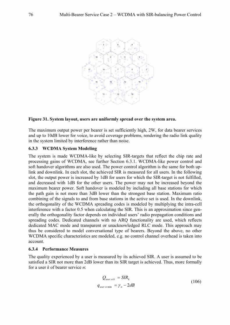
76 Multi-Bearer Service Case 2 – WCDMA with SIR-balancing Power Control
The maximum output power per bearer is set sufficiently high, 2W, for data bearer services and up to 10dB lower for voice, to avoid coverage problems, rendering the radio link quality in the system limited by interference rather than noise.
6.3.3 WCDMA System Modeling The system is made WCDMA-like by selecting SIR-targets that reflect the chip rate and processing gains of WCDMA, see further Section 6.3.1. WCDMA-like power control and soft handover algorithms are also used. The power control algorithm is the same for both up-link and downlink. In each slot, the achieved SIR is measured for all users. In the following slot, the output power is increased by 1dB for users for which the SIR-target is not fulfilled, and decreased with 1dB for the other users. The power may not be increased beyond the maximum bearer power. Soft handover is modeled by including all base stations for which the path gain is not more than 3dB lower than the strongest base station. Maximum ratio combining of the signals to and from base stations in the active set is used. In the downlink, the orthogonality of the WCDMA spreading codes is modeled by multiplying the intra-cell interference with a factor 0.5 when calculating the SIR. This is an approximation since gen-erally the orthogonality factor depends on individual users’ radio propagation conditions and spreading codes. Dedicated channels with no ARQ functionality are used, which reflects dedicated MAC mode and transparent or unacknowledged RLC mode. This approach may thus be considered to model conversational type of bearers. Beyond the above, no other WCDMA specific characteristics are modeled, e.g. no control channel overhead is taken into account.
6.3.4 Performance Measures The quality experienced by a user is measured by its achieved SIR. A user is assumed to be satisfied a SIR not more than 2dB lower than its SIR target is achieved. Thus, more formally for a user k of bearer service n:
dBq
SIRQ
nnuser
kknuser
2min −=
=
γ (106)
1
2
3
4
5
6
7
8
9
10
11
12
13
14
15
16
17
18
19
Figure 31. System layout, users are uniformly spread over the system area.
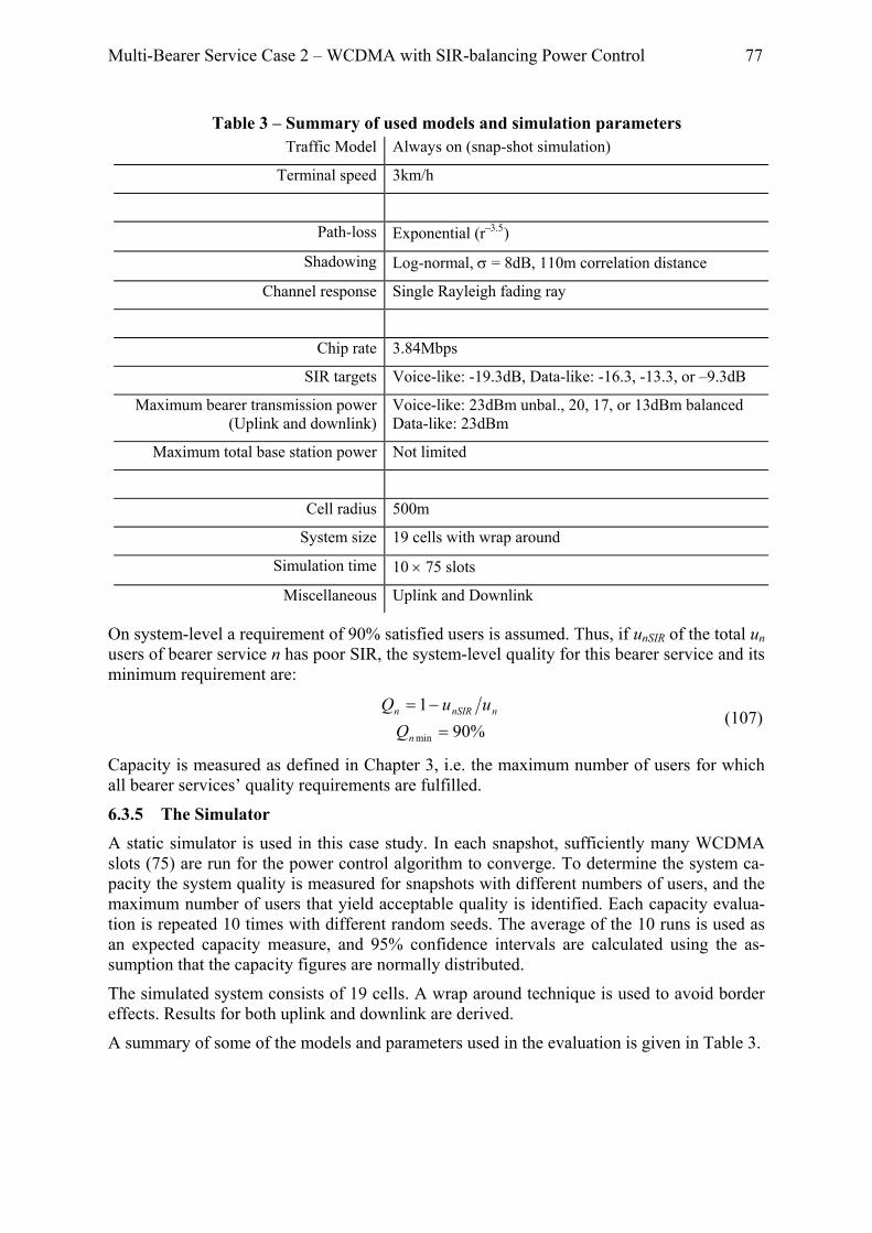
Multi-Bearer Service Case 2 – WCDMA with SIR-balancing Power Control 77
On system-level a requirement of 90% satisfied users is assumed. Thus, if unSIR of the total un users of bearer service n has poor SIR, the system-level quality for this bearer service and its minimum requirement are:
%90
1
min =−=
n
nnSIRn
QuuQ
(107)
Capacity is measured as defined in Chapter 3, i.e. the maximum number of users for which all bearer services’ quality requirements are fulfilled.
6.3.5 The Simulator
A static simulator is used in this case study. In each snapshot, sufficiently many WCDMA slots (75) are run for the power control algorithm to converge. To determine the system ca-pacity the system quality is measured for snapshots with different numbers of users, and the maximum number of users that yield acceptable quality is identified. Each capacity evalua-tion is repeated 10 times with different random seeds. The average of the 10 runs is used as an expected capacity measure, and 95% confidence intervals are calculated using the as-sumption that the capacity figures are normally distributed.
The simulated system consists of 19 cells. A wrap around technique is used to avoid border effects. Results for both uplink and downlink are derived.
A summary of some of the models and parameters used in the evaluation is given in Table 3.
Table 3 – Summary of used models and simulation parameters Traffic Model Always on (snap-shot simulation)
Terminal speed 3km/h
Path-loss Exponential (r−3.5)
Shadowing Log-normal, σ = 8dB, 110m correlation distance
Channel response Single Rayleigh fading ray
Chip rate 3.84Mbps
SIR targets Voice-like: -19.3dB, Data-like: -16.3, -13.3, or –9.3dB
Maximum bearer transmission power (Uplink and downlink)
Voice-like: 23dBm unbal., 20, 17, or 13dBm balanced Data-like: 23dBm
Maximum total base station power Not limited
Cell radius 500m
System size 19 cells with wrap around
Simulation time 10 × 75 slots
Miscellaneous Uplink and Downlink

78 Multi-Bearer Service Case 2 – WCDMA with SIR-balancing Power Control
6.4 Numerical Results In this section simulated and theoretical capacity regions are compared with and without in-terference balancing, for both uplink and downlink, and for differences in SIR target be-tween bearer services of 3, 6, and 10dB. When deriving the theoretical results, the scenario of Section 4.3.1 is assumed to be valid.
Figure 32 shows downlink results for a difference in SIR target of 3dB. Unbalanced results are shown in the left plots, and balanced results in the right plots. The top plots show the fraction of satisfied users as a function of the estimated expected interference level in the system. In both the balanced and unbalanced cases it is seen that the maximum interference levels imax1 and imax2 are rather independent of service mix (the different curves of same color and legend). In the unbalanced case the different bearer services have different maximum interference levels, imax1 > imax2. As in the GERAN case, this is because bearer service 1 with its 3dB lower SIR requirement can stand a 3dB higher interference level before its users run out of transmission power. In the balanced case, the maximum bearer power levels are ad-justed so the maximum interference levels are equal, imax1 = imax2. This is accomplished through lowering the maximum power of the bearer service with the lower SIR target by 3dB.
The middle plots show how the interference levels increase with the number of users in the single-bearer service scenarios for both bearer services. The single-bearer service capacities Csingle1 and Csingle2, i.e. the number of users at the maximum interference level, for each bearer service are highlighted. Note again that in the balanced case the maximum interfer-ence levels are equal.
According to the theory of Section 4.3.1, the capacity region should be delimited by a straight line between the number of users at the smallest of the two maximum interference levels, i.e. between u1(min{imax1, imax2}) and u2(min{imax1, imax2}). Note that as in the GSM/EDGE case, with unbalanced interference levels, one of these endpoints are open. In this case, since imax1 > imax2, it is the point u1(min{imax1, imax2}). In a strictly bearer service 1-only system, the interference can be increased beyond what is tolerable for bearer service 2-users. However, as soon as a small fraction of bearer service 2-users is introduced, the inter-ference must be decreased and the number of bearer service 1-users must be decreased to u1(min{imax1, imax2}) is approached. This is also the explanation for the discontinuity in the theoretical capacity region when the fraction of bearer service 2-users increases from zero to just above zero.
The bottom plots show a comparison between such theoretical capacity regions and simu-lated ones including 95% confidence intervals. By comparing the unbalanced and balanced plots the gain achieved by the interference balancing can also be seen. A reasonably good agreement between simulation and theory is observed. This likely depends on the necessary assumptions holding in this case, i.e. the system is interference-limited, and the maximum tolerable interference and the interference contribution per user is largely independent of the service mix.
An identical analysis for the uplink is presented in Figure 33. The conclusions are the same; a gain is achieved by interference balancing, and the simulated results and theoretical results agree quite well. The uplink gain is however smaller than what is achieved for the downlink. As discussed in Section 4.3.1.1, this occurs because the interference grows more rapidly with the traffic load in the uplink than in the downlink. This is also the explanation for the gain

Multi-Bearer Service Case 2 – WCDMA with SIR-balancing Power Control 79
being smaller than that for GSM/EDGE seen in the previous case study. The interference grows more rapidly with traffic load for WCDMA than for GSM/EDGE.
Downlink and uplink capacity regions before and after interference balancing with differ-ences in SIR targets of 6 and 10dB are shown in Figure 34 and Figure 35 respectively. In these cases larger capacity gains are achieved by interference balancing. The gain grows with the difference in SIR target. This depends on the larger difference between the maxi-
-100 -95 -90 -85 -80 -75 -70 -6580
85
90
95
100
Estimated Expected Downlink Interference [dBm]
Frac
tion
of S
atis
fied
Use
rs [%
]
Service 1Service 2
Q1min= Q2min
imax2 imax1
-100 -95 -90 -85 -80 -75 -70 -6580
85
90
95
100
Estimated Expected Downlink Interference [dBm]
Frac
tion
of S
atis
fied
Use
rs [%
]
Service 1Service 2
imax1
Q1min= Q2min
imax2
0 20 40 60 80 100-100
-95
-90
-85
-80
-75
-70
-65
Number of Users
Estim
ated
Exp
ecte
d D
ownl
ink
Inte
rfere
nce
[dB
m]
Service 1Service 2
imax1
imax2
Csingle 2 Csingle 1
0 20 40 60 80 100-100
-95
-90
-85
-80
-75
-70
-65
Number of Users
Estim
ated
Exp
ecte
d D
ownl
ink
Inte
rfere
nce
[dB
m]
Service 1Service 2
imax1imax2
Csingle 2 Csingle 1
0 10 20 30 40 50 60 70 800
5
10
15
20
25
30
35
40
Service 1 Users
Serv
ice
2 U
sers
SimulationTheory
0 10 20 30 40 50 60 70 800
5
10
15
20
25
30
35
40
Service 1 Users
Serv
ice
2 U
sers
SimulationTheory
Figure 32. Comparisons of theoretical results with simulated downlink WCDMA results without interference balancing (left) and with interference balancing (right). The differ-ence in SIR target between bearer service 1 and 2 is 3dB.
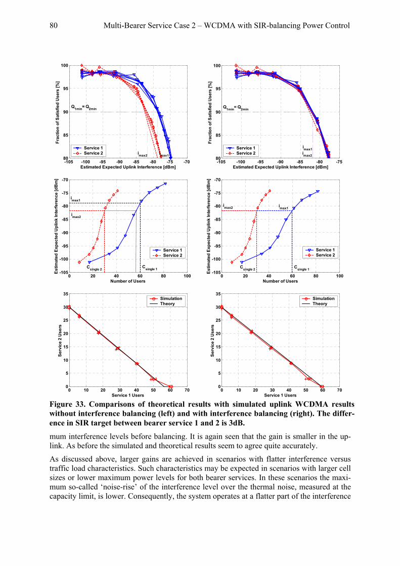
80 Multi-Bearer Service Case 2 – WCDMA with SIR-balancing Power Control
mum interference levels before balancing. It is again seen that the gain is smaller in the up-link. As before the simulated and theoretical results seem to agree quite accurately.
As discussed above, larger gains are achieved in scenarios with flatter interference versus traffic load characteristics. Such characteristics may be expected in scenarios with larger cell sizes or lower maximum power levels for both bearer services. In these scenarios the maxi-mum so-called ‘noise-rise’ of the interference level over the thermal noise, measured at the capacity limit, is lower. Consequently, the system operates at a flatter part of the interference
-105 -100 -95 -90 -85 -80 -75 -7080
85
90
95
100
Estimated Expected Uplink Interference [dBm]
Frac
tion
of S
atis
fied
Use
rs [%
]
Service 1Service 2
Q1min= Q2min
imax2 imax1
-105 -100 -95 -90 -85 -80 -7580
85
90
95
100
Estimated Expected Uplink Interference [dBm]
Frac
tion
of S
atis
fied
Use
rs [%
]
Service 1Service 2
Q1min= Q2min
imax2
imax1
0 20 40 60 80 100-105
-100
-95
-90
-85
-80
-75
-70
Number of Users
Estim
ated
Exp
ecte
d U
plin
k In
terfe
renc
e [d
Bm
]
Service 1Service 2
imax1
imax2
Csingle 2 Csingle 1
0 20 40 60 80 100-105
-100
-95
-90
-85
-80
-75
-70
Number of Users
Estim
ated
Exp
ecte
d U
plin
k In
terfe
renc
e [d
Bm
]
Service 1Service 2
imax1imax2
Csingle 2 Csingle 1
0 10 20 30 40 50 60 700
5
10
15
20
25
30
35
Service 1 Users
Serv
ice
2 U
sers
SimulationTheory
0 10 20 30 40 50 60 700
5
10
15
20
25
30
35
Service 1 Users
Serv
ice
2 U
sers
SimulationTheory
Figure 33. Comparisons of theoretical results with simulated uplink WCDMA results without interference balancing (left) and with interference balancing (right). The differ-ence in SIR target between bearer service 1 and 2 is 3dB.

Multi-Bearer Service Case 2 – WCDMA with SIR-balancing Power Control 81
versus traffic load curve; see e.g. the middle row plots of Figure 32 and Figure 33. Hence, larger capacity gains may be expected.
6.5 Summary As for GSM/EDGE, interference balancing may be achieved for power controlled WCDMA bearers by adjusting the maximum bearer output power. This is valid for both the downlink and uplink. Linear capacity regions are achieved for the range of evaluated differences in SIR targets (up to 10dB). For the downlink, capacity gains ranging from about 15% for a 3dB difference in SIR target to about 25% for a 10dB SIR target difference are achieved. For the uplink, the gains range from about 10% to about 16%. The smaller gain for the uplink is due to steeper interference versus traffic load characteristics for the uplink than the downlink. Further, for a given difference in SIR requirement, the WCDMA gains are smaller than what is achieved for GSM/EDGE. Also this is due to the steeper interference versus traffic load characteristics for the SIR-balancing power controlled WCDMA bearers than for the GSM/EDGE bearers.
0 10 20 30 40 50 60 70 800
5
10
15
20
Service 1 Users
Serv
ice
2 U
sers
SimulationTheory
Before Balancing
After Balancing
0 10 20 30 40 50 60 700
2
4
6
8
10
12
14
16
Service 1 Users
Serv
ice
2 U
sers
SimulationTheory
Before Balancing
After Balancing
Figure 34. Comparisons of theoretical results with simulated WCDMA results before and after interference balancing for downlink (left) and uplink (right). The difference in SIR target between bearer service 1 and 2 is 6dB.
0 10 20 30 40 50 60 70 800
1
2
3
4
5
6
7
8
Service 1 Users
Serv
ice
2 U
sers
SimulationTheory
Before Balancing
After Balancing
0 10 20 30 40 50 60 700
1
2
3
4
5
6
Service 1 Users
Serv
ice
2 U
sers
SimulationTheory
Before Balancing
After Balancing
Figure 35. Comparisons of theoretical results with simulated WCDMA results before and after interference balancing for downlink (left) and uplink (right). The difference in SIR target between bearer service 1 and 2 is 10dB.


83
Chapter 7 Multi-Bearer Service Case 3 – Voice and WWW in WCDMA/HSDPA
In this chapter the interference balancing principles of Chapter 4 are applied to a mixed voice and WWW WCDMA/HSDPA system. First, an overview of the HSDPA concept is given. This is followed by a description of how interference balancing can be realized for WCDMA/HSDPA. Models and assumptions specific to this case study are then defined, be-fore the numerical results are presented. Scenarios with different quality requirements, bearer realizations, and radio environments are evaluated before and after interference bal-ancing. The results are also compared to the expected results of Section 4.3.
7.1 HSDPA Overview The High-Speed Downlink Packet Access (HSDPA) concept is a new set of functions added to the release 5 of the 3GPP WCDMA standard. A thorough presentation of the concepts is provided e.g. in [120]. Very briefly, a new Transport Channel, see Section 6.1, denoted High-Speed Downlink Shared Channel (HS-DSCH) is introduced. Up to ¾ of the code tree of a WCDMA carrier may be allocated to the HS-DSCH. The remaining codes may be used for other channels, e.g. Dedicated Channels (DCH) for voice bearers. The HS-DSCH differs from the standard Downlink Shared Channel (DSCH) mainly in that it supports faster sched-uling, link adaptation, and incremental redundancy.
Faster scheduling is enabled through introduction of a Transmission Time Interval (TTI) of 2ms for the HS-DSCH, as compared to 10ms for the DSCH. The TTI is the smallest unit of time a user is allocated to the HS-DSCH. Typically only one user at a time is scheduled on the HS-DSCH, although sharing of the HS-DSCH codes is possible. The short TTI together with rapid feedback of channel conditions means that it is possible to track changes in multi-path fading. For example, to improve system throughput it is possible to schedule data for the user with the currently highest instantaneous SIR. Alternatively, an element of user fair-ness may be added by scheduling data for the user with the highest ratio between instantane-ous SIR and average SIR. This is sometimes denoted proportional fair scheduling.
In addition to the regular WCDMA QPSK modulation, the HS-DSCH also supports 16QAM modulation. A variety of different channel code rates are also supported. Combining these, peak data rates up to 15Mbps are achievable. Through the use of link adaptation, the combi-nation of modulation and channel coding most appropriate for each user may be selected. The link adaptation may target maximized bitrate or minimized delays. The link adaptation operates on TTI-level.
The HS-DSCH performance is also enhanced by incremental redundancy. In short this means that the receivers are able to combine soft information from successive decoding at-tempts of a data frame. The result is that the cumulative error probability decreases for every retransmission of a block, which in turn increases the bitrate and decreases delays compare to conventional ARQ schemes. The decreasing error probability also means that the re-quirements on accurate link adaptation are relaxed.

84 Multi-Bearer Service Case 3 – Voice and WWW in WCDMA/HSDPA
Figure 36 depicts the basic HSDPA principles. In addition to these, the amount of power al-located to the HS-DSCH is an important factor in multi-bearer service scenarios. This is dis-cussed in the next section.
7.2 Interference Balancing in WCDMA/HSDPA In this study it is assumed that dedicated channels and control channels have priority over the HS-DSCH when allocating power. This is motivated by the less stringent requirements on instantaneous quality for the bearer service carried by the HS-DSCH compared to dedi-cated channels and control channels. Thus, in every slot control channels and dedicated channels are first allocated the power they need to fulfill their SIR targets using regular power control mechanisms. The aggregate power required for these channels is denoted Pother. The HS-DSCH is then allocated the remaining base station power up to a threshold Pth. Hence:
otherthDSCHHS PPP −=− (108)
The maximum interference level tolerated by users of the HS-DSCH may be controlled by adjusting Pth. As discussed in the previous chapter, the maximum interference tolerated by users of dedicated channels may be controlled by adjusting the maximum bearer power Pmax. Hence, interference balancing may be achieved by adjusting Pth and Pmax so that the maxi-mum interference levels become equal. Noticeably, several combinations of Pth and Pmax may achieve interference balancing. Further, due to the varying power allocated to the HS-DSCH, it is difficult to analytically associate the threshold power Pth with maximum toler-ated interference levels, and further with maximum dedicated channel bearer powers Pmax. In this study these are instead empirically derived. An approach is used where Pth is set to the maximum base station power, i.e. Pth = 20W, and the maximum voice bearer power Pmax is first set to a value that is expected to be sufficient to cope with the resulting interference lev-els. The maximum voice bearer power Pmax is then gradually lowered until interference bal-ancing is achieved.
SF=4
SF=2
SF=1
HS-DSCH Other channels
tUser 1
2ms
User 2 User 2 User 3 User 1 User 3
SF=16
SF=8
-5 0 5 100
1
2
3
4
5
6
7
8
SIR [dB]
Link
Thr
ough
put [
Mbp
s]
QPSK R=0.25
QPSK R=0.5
16QAM R=0.38
16QAM R=0.63
Figure 36. HSDPA principles. A part of the code tree, in this example 12/16, is allo-cated to the HS-DSCH. The HS-DSCH is shared between users in the time domain, scheduling of users may be based e.g. on channel quality. Modulation and coding schemes are selected individually for each user, e.g. to maximize data rates or minimize delays.

Multi-Bearer Service Case 3 – Voice and WWW in WCDMA/HSDPA 85
7.3 Models and Assumptions This section presents and discusses the models and assumptions used in this case study. A summary is given in the end of the section in Table 4.
7.3.1 User Behavior Modeling As in the GSM/EDGE case study, users of voice and WWW type are studied. A user is ex-clusively of one type, i.e. no multi-media users are included. Spatially, both voice and WWW users are assumed to be located according to a uniform distribution within the system area. Both voice and WWW users are further assumed to move with an average speed of 3km/h.
The number of voice users in the system is assumed to be fixed for each studied load. Hence, no users enter or leave the system during the period of observation. The duration of a voice call is further assumed to be infinite.
Similarly, the number of WWW users in the system is assumed to be fixed for each studied load, and the session time is assumed to be infinite. Within a session, a WWW user requests a new HTML page a certain reading time after the previous HTML page was delivered. The reading time is assumed to be exponentially distributed with an expectation of 5s. The size of the HTML pages follows a truncated lognormal distribution. The expected page size is 17.2kbytes, and the minimum and maximum sizes are 1kbyte and 200kbytes respectively. Note that division of HTML pages into HTTP objects is not included in the model. Alto-gether, assuming a negligible transmission time this results in an expected traffic load per user of 27.5kbps. In practice, with non-zero transmission times, this figure becomes lower. The number of voice and WWW users is varied to study different traffic loads and service mixes. The above traffic models are kept relatively simple to limit simulation times. For ex-ample, no TCP model is included in the evaluation. Evaluations including TCP effects are reported in [93]. A capacity loss of about 10% is seen when introducing the TCP model, mainly due to the TCP slow-start phase.
7.3.2 Radio Network Modeling A system with three-sector sites placed on a regular grid is assumed. The cell radius is 500m. Pathloss is exponentially modeled with an exponent of 3.52, and shadow fading is log-normally modeled with standard deviation 8dB and a correlation distance of 100m. Multi-path fading is modeled using either the rather non-dispersive UMTS Pedestrian A channel model, with three resolvable paths with relative energy levels of -0.2, -13, and –25dB, or the more time-dispersive 3GPP Typical Urban channel model with 12 resolvable paths with rela-tive energies linearly decreasing from –4dB to –24dB [121].
7.3.3 WCDMA and HSDPA Modeling
Rather accurate models of the WCDMA radio interface are used. From a bearer realization and protocol perspective, voice bearers are assumed to be realized using the transparent RLC mode, the dedicated MAC mode, and using dedicated transport channels. The user plane functionality of these RLC and MAC modes is largely limited to passing incoming data units to the next lower layer. This is modeled through passing incoming speech frames directly to the physical layer. The channel coding and modulation of the physical layer are directly im-plemented as specified in the 3GPP standards. A spreading factor of 128 and a Transmission Time Interval (TTI) of 20ms are used. For simplicity, DTX is not used in most evaluated scenarios. Some results with DTX are presented in Appendix F.

86 Multi-Bearer Service Case 3 – Voice and WWW in WCDMA/HSDPA
WWW bearers use PDCP, the acknowledged RLC mode, shared MAC mode and the High-Speed Downlink Shared Channel (HS-DSCH). As in the GSM/EDGE case, the header com-pression functionality of the PDCP layer is not modeled. This simplification is also in this case expected to have a minor effect on the results. On the RLC layer functionality for seg-mentation and reassembly as well as ARQ are modeled. The 4-channel staggered stop-and-wait ARQ mechanism used for the HS-DSCH is implemented in detail. A roundtrip time of 8ms is assumed. The MAC layer implements only one-by-one scheduling. Scheduling multi-ple users simultaneously on different parts of the code tree allocated to the HS-DSCH is supported by the standard, but not used in the evaluations. In accordance with the standard 2ms TTIs are used. As for the voice bearers, the parameters of the physical layer are directly implemented as standardized. A total of 12 codes with spreading factor 16, i.e. ¾ of the code tree, are assumed to be allocated to the HS-DSCH. For simplicity this is done regardless of the number of voice users in the system. For large number of voice users, which requires more than ¼ of the codes allocated to voice bearers and control channels, this HS-DSCH code allocation is not realistic. However, the effect on the capacity results is limited, since for a high number of voice users the power allocated to the HS-DSCH is so low, that it is power rather than bandwidth limited, and thus its performance does not depend much on the number of allocated codes.
The radio interface control plane is included in the modeling. Broadcast and common control channels are assumed to be continuously transmitted from each base station with a constant output power of 4W. Each WWW user further has an associated dedicated control channel for transmitting e.g. scheduling information in the downlink and ARQ reports in the uplink. These channels are included in the modeling and are assumed to have a spreading factor 256. The modeling is limited to allocating power to these channels. Errors on the associated channels are not taken into account.
Apart from models reflecting the WCDMA standard, radio resource management solutions are also modeled. For voice bearers an SIR balancing power control with a step size of 1dB and a nominal SIR target of –19.3dB is assumed. A measurement error of the SIR estimates are assumed to follow a lognormal distribution with a standard deviation of 5dB. The SIR target is regulated with an outer power control loop targeting a frame erasure rate of 0.7%. Soft handover is assumed for voice bearers and the associated control channels for WWW users. A base station is added to the active set if its signal strength is within 2dB of the strongest base station, and removed if its signal strength falls below 4dB less than the strongest base station. No admission or congestion control is assumed. For WWW users, the HS-DSCH is allocated power according to Equation (108). Round Robin scheduling within each base station is assumed. No coordinated inter-cell scheduling is performed. In each TTI the modulation and coding scheme maximizing the expected bitrate for the estimated link
Non-transparent
Dedicated
PDCP
RLC
MAC
Transparent
Phy HS-DSCH
Acknowledged
Shared
Voice WWW
DCH
Not modeled
Modeled
Modeled
Modeled
Modeled
Modeled
Modeled Figure 37. Protocol modes assumed for the voice and WWW bearers. The modeling of each layer is also indicated.

Multi-Bearer Service Case 3 – Voice and WWW in WCDMA/HSDPA 87
quality (based on SIR) is selected. This principle is depicted in Figure 36 (right). The round-trip time for receiving SIR estimates is assumed to be 4ms. In this case, the SIR measure-ment error is assumed follow a lognormal distribution with a standard deviation of 4dB.
7.3.4 Performance Measures
The performance measures defined in Section 5.3.4 for the GSM/EDGE case study are also used in this case study. The only difference is that here the minimum CSE bitrate required for a WWW user to be satisfied is assumed to be 50kbps. Additionally, some results with CSE bitrate requirements of 150 and 300kbps are presented in Appendix F.
7.3.5 The Simulator A dynamic multiple cell system simulator is used. The simulated system consists of 7 three-sector sites, yielding a total of 21 sectors. A wrap-around technique is used to avoid border effects. The simulator operates on WCDMA slot-level (0.67ms). In every time-step of the simulation the SIR before despreading is measured and the Eb/I0 after despreading is calcu-lated for each link. When all slots of a frame are received (30 for voice bearers and 3 for HS-DSCH), a Frame Erasure Rate (FER) is extracted based on the measures for the included slots together with previously simulated Eb/I0 to FER relations. For voice bearers, the FER values are logged and used for performance evaluations. For the HS-DSCH, a random ex-periment is made such that a frame is erroneous and needs to be retransmitted with a prob-ability equal to the calculated FER, and is successfully received with probability 1-FER.
Table 4 – Summary of models and simulation parameters HTML page size Lognormal, µ=17.2kbyte, [min, max] = [1, 200] kbytes
Reading time between HTML pages Exponential, µ=5s
WWW load per user during session 27kbps if transmission times negligible
Voice call duration Infinite
Voice activity factor 1 (no DTX)
Mobile speed 3km/h
Path-loss Exponential (rσ), α = 3.52
Shadowing Log-normal, σ = 8dB
Channel response 3GPP Pedestrian A or 3GPP Typical Urban
HS-DSCH Scheduling Round-Robin
System size 21 sectors
Simulation time 3 × 100s with different random seeds
Miscellaneous Downlink

88 Multi-Bearer Service Case 3 – Voice and WWW in WCDMA/HSDPA
7.4 Numerical Results This section presents simulated capacity regions with and without interference balancing. The numerical results are also compared to what is expected from the theory of Chapter 4. Two scenarios with different channel models are evaluated; in the first scenario the 3GPP Pedestrian channel is used, and in the second scenario the 3GPP Typical Urban channel is used. In both scenarios the HS-DSCH is allocated all the remaining base station power, i.e. Pth = 20W, and the maximum voice bearer power is varied to balance interference levels. Results with alternative CSE bitrate requirements as well as voice bearers using DTX are presented in Appendix F.
7.4.1 Scenario 1 – 3GPP Pedestrian A Channel In this scenario, to begin with, a maximum voice bearer power of 14W is used, which is ex-pected to be sufficient to cope with the interference from the HS-DSCH and the strongly fad-ing Pedestrian A channel. Figure 38 (left) shows the maximum interference level for voice and data plotted versus the fraction of voice users. The total base station output power is used as a measure of the interference in the system. It is seen that the maximum interference tolerated by data bearers is relatively constant and around 19.5W. The maximum interfer-ence tolerated by the voice bearers however varies with the service mix. For large fractions of voice users a lower interference level is tolerated; the maximum interference level is 13W in the single-bearer service case, whereas it is greater than the maximum base station output power of 20W for fractions of voice users below 0.5 (the plot is truncated at 20W). The rea-son for this is that for higher fractions of voice users, the absolute number of voice users sharing the common power budget is larger, and each user is less likely to get the required power. Figure 38 (right) shows the interference contribution per user, measured at the capac-ity limit, for voice and data plotted versus the fraction of voice users. It is seen that for voice the interference contribution is independent of the service mix. For data on the other hand, the interference contribution is lower for high fractions of voice users, or equivalently lower fractions of data users. This may be explained by the fact that there is less queuing given that there are fewer data users in the system. This results in a longer transmission time being al-
0 0.2 0.4 0.6 0.8 113
14
15
16
17
18
19
20
Service Mix (λv)
Max
imum
Sus
tain
able
Dow
nlin
k Po
wer
[W]
Pmax DPmax V
0 0.2 0.4 0.6 0.8 1-2.5
-2
-1.5
-1
-0.5
0
0.5
Service Mix (λv)
Rel
ativ
e D
ownl
ink
Pow
er U
sage
per
Use
r [dB
]
VoiceData
Figure 38. Left: Maximum voice and data interference levels (measured as total downlink power) as a function of service mix. Left: Interference contribution per user (measured as downlink power usage) as a function of service mix. (Pedestrian A sce-nario)

Multi-Bearer Service Case 3 – Voice and WWW in WCDMA/HSDPA 89
lowed while still fulfilling the QoS requirements, which in turn leads to a lower required power.
The resulting capacity region is shown in Figure 39. As might be expected from the maxi-mum tolerable interference level versus service mix characteristics, see example 3 in Section 4.3.2, a convex capacity region is achieved. Intuitively, this is because at the capacity limit in a single-bearer service voice system, there is a rather large average power budget (20W-13W = 7W) not used by the voice bearers. This power may be used by the HS-DSCH to provide a significant data capacity even for voice loads only slightly lower than the single-bearer ser-vice voice capacity. Indeed, using this power the data bearers interfere with the voice bear-ers. However, a small reduction of the number of voice users seems to be sufficient for the voice bearers to cope with this increased interference.
A comparison of the simulated results with the theoretically derived results is also provided in Figure 39. In the theoretical case, since both the maximum interference levels and inter-ference contribution per user depend on the service mix, the scenario of Section 4.3.3 is as-sumed. Hence, Equation (63) is used together with the interference tolerance levels and in-terference contributions depicted in Figure 38. It is seen that the theory quite accurately to explains the simulated results. Note however that the theoretical results in this case may not be considered to predict the simulated results, as the maximum interference levels, which are a necessary input, are a result of the simulation.
In the above example no attempts to balance interference levels are made. As seen in Figure 38 (right), for high fractions of voice users, the voice tolerates less interference than data, whereas for small fractions of voice users the situation is the opposite. For small fractions of voice users the maximum voice bearer power could hence be reduced to allocate additional power for the HS-DSCH, and hence provide higher capacity.
The effect on the maximum interference levels of reducing the maximum voice bearer power from 14W to 6W and 3W is depicted in the left plot in Figure 40. In the 6W-case, it is seen that despite the decrease in maximum power, interference levels corresponding to output powers larger than 20W are still sustainable for low fractions of voice users. Hence, the in-terference tolerance for voice has not been reduced too much. Further reduction of the maxi-mum voice bearer power to 3W however renders dramatically poorer voice quality; and the
0 1 2 3 4 5 60
50
100
150
200
250
300
350
Voice Capacity [Erlang/MHz/Sector]
WW
W C
apac
ity [k
bps/
MH
z/Se
ctor
]
SimulationTheory
Figure 39. Simulated and theoretical voice and WWW capacity regions for the Pedes-trian A case.

90 Multi-Bearer Service Case 3 – Voice and WWW in WCDMA/HSDPA
voice bearer service becomes limiting. This indicates that a maximum voice bearer power of 6W is reasonably appropriate from an interference balancing perspective.
Somewhat surprisingly it is also seen that with a maximum bearer power for voice of 6W, the maximum interference level for voice actually increases for high fractions of voice users. This may be seen as a paradox since the maximum power level for voice bearers has been decreased. The explanation lies in the limiting of the total base station output power. After each iteration of the power control algorithm, if the sum of the voice bearer power levels causes the total base station power to exceed its maximum of 20W, the power is decreased with a common factor for all voice bearers so that the total power becomes 20W. Whenever this event takes place, all voice bearers fail to reach their SIR targets, and experience re-duced quality. With a high maximum power, this event becomes more frequent, and the re-duction in power in each event also increases. In summary, a higher maximum power may benefit single users with poor radio conditions, but often does this by sacrificing the quality for the majority of the users, whereas a lower maximum power protects the majority of the users from power consuming users in poor radio conditions.
The resulting capacity regions are shown in the right plot in Figure 40. With a maximum bearer power for voice of 6W, as might be expected from the maximum interference level characteristics, the capacity is increased for all service mixes, including the voice-only case. With a maximum voice bearer power of 3W, significantly worse mixed bearer service per-formance is achieved. The single-bearer service voice capacity is also somewhat lower. This result points to the attractive property of that the maximum voice bearer power that is used to balance interference levels also may be used to improve single-bearer service voice capacity. Also note that the theory may also in this case quite accurately explain the shape of the simu-lated capacity region (only shown for the 6W case).
7.4.2 Scenario 2 – 3GPP Typical Urban Channel The above analysis is also done with a 3GPP Typical Urban channel. Figure 41 (left) shows the same plot as Figure 38 (right), but for the Typical Urban scenario. The maximum voice bearer power is again initially set to 14W. The results are similar to the Pedestrian scenario, with the exception that the voice bearers are even more robust. The increased robustness is due to the diversity offered by the multiple paths of the Typical Urban channel. In the single-
0 0.2 0.4 0.6 0.8 110
12
14
16
18
20
Service Mix (λv)
Max
imum
Sus
tain
able
Dow
nlin
k Po
wer
[W]
Imax D (14W)Imax V(14W) Imax D (6W) Imax V(6W) Imax D (3W) Imax V(3W)
0 1 2 3 4 5 6 70
50
100
150
200
250
300
350
Voice Capacity [Erlang/MHz/Sector]
WW
W C
apac
ity [k
bps/
MH
z/Se
ctor
]
SimulationTheory
PmaxV= 14W
PmaxV= 6W
PmaxV= 3W
Figure 40. The effect of interference balancing in the Pedestrian A scenario. Left: Maxi-mum interference levels as a function of service mix. Right: Simulated and theoretical capacity regions with different maximum voice bearer power levels.

Multi-Bearer Service Case 3 – Voice and WWW in WCDMA/HSDPA 91
bearer service voice case, an interference level of about 17W is tolerated, and already at a normalized fraction of voice users of 0.75, the maximum interference level exceeds 20W (the plot is truncated at 20W). The reason for this behavior is the same as in the Pedestrian scenario; more power is available per voice bearer for smaller fractions of voice user, which yields a higher interference tolerance. The maximum interference level for data is rather con-stant around 19W.
Figure 41 (right) shows the resulting capacity region. As in the Pedestrian scenario the ca-pacity region is convex, which is explained by the shape of maximum interference versus service mix characteristics. The convexity knee at high fractions of voice users is a little less evident, which is due to the smaller increase in maximum interference levels compared to the voice-only case, 19W-17W = 2W in this scenario. The comparison with the theoretical results, derived in the same manner as in the Pedestrian case, again shows that the theory may quite accurately explain the shape of the capacity region.
As in the Pedestrian scenario, no attempt to balance interference levels are made in the above example. Since the maximum interference level for data is limiting for all service mixes, ex-cept voice-only, a capacity gain could be achieved by reducing the maximum voice bearer power. As seen in Figure 42 (left), for a maximum voice bearer power of 1W, the maximum interference level for voice is still as high as 20W for large fractions of data users, and, for the same reasons as in the Pedestrian A scenario, also increased for high fractions of voice users. Decreasing the maximum voice bearer power to 0.5W however dramatically reduces the tolerable interference levels The resulting capacity regions are compared to the one achieved with Pmax v=14W in Figure 42 (right). It is seen that with Pmax v=1W a rather signifi-cant capacity gain can be achieved for high fractions of voice users. However, for lower fractions of voice users no gain is achieved. This is because for small fractions of voice us-ers, the number of voice users that decrease their power is small, and the increase in power available for the HS-DSCH is limited. For high fractions of voice users the situation is the opposite. As in the Pedestrian A scenario, a gain in single-bearer service voice capacity is also achieved for the same maximum voice bearer power that is used to balance interference levels. As expected from the maximum interference levels, poor performance is achieved with Pmax v=0.5W.
Some additional results with varying CSE bitrate requirements for WWW users and voice bearers with DTX functionality are presented in Appendix F.
0 0.2 0.4 0.6 0.8 116.5
17
17.5
18
18.5
19
19.5
20
Service Mix (λv)
Max
imum
Sus
tain
able
Dow
nlin
k Po
wer
[W]
Pmax DPmax V
0 1 2 3 4 5 6 7 80
50
100
150
200
250
Voice Capacity [Erlang/MHz/Sector]
WW
W C
apac
ity [k
bps/
MH
z/Se
ctor
]
SimulationTheory
Figure 41. Left: Maximum voice and data interference levels as a function of service mix. Right: Simulated and theoretical capacity region. (Typical Urban scenario)

92 Multi-Bearer Service Case 3 – Voice and WWW in WCDMA/HSDPA
7.5 Summary Interference balancing between power controlled dedicated bearers and HS-DSCH-based bearers in WCDMA can be achieved by adjusting the maximum bearer power for the dedi-cated bearers and the maximum total base station power when the HS-DSCH is transmitted. However, the gain is quite limited. There are different reasons for this. First, in the reference case the system already performs very well and is close to balanced. As compared to the previous case studies for which normalized capacities of c( λ
r) = 1.0 were achieved after in-
terference balancing, convex capacity regions with c( λr
) > 1.0 are in this case study already achieved before interference balancing is introduced. Secondly, due to the power allocation rule that prioritizes voice bearers, it is not always possible to make the data bearer tolerate as much interference as voice the bearers, thus perfect balancing can not always be achieved. Finally, the interference to traffic load characteristics are relatively steep, which means that a balanced interference translates to a small number of users. It is further seen that the interfer-ence balancing realizations depend on the channel model, which is unattractive if the channel type is not known or differs within cells. A straightforward solution that performs well for most bearer service mixes is to make sure the maximum voice bearer power is sufficiently high and then allocate all the remaining base station power to the HS-DSCH. The resulting capacity regions are convex. This depends on that the voice bearers tolerate more interfer-ence the fewer in number they are, which in turn depends on their common shared power budget.
0 0.2 0.4 0.6 0.8 18
10
12
14
16
18
20
Service Mix (λv)
Max
imum
Sus
tain
able
Dow
nlin
k Po
wer
[W]
Imax D (14W) Imax V(14W) Imax D (1W) Imax V(1W) Imax D (0.5W)Imax V(0.5W)
0 2 4 6 8 100
50
100
150
200
250
Voice Capacity [Erlang/MHz/Sector]
WW
W C
apac
ity [k
bps/
MH
z/Se
ctor
]
SimulationTheory
PmaxV= 14W PmaxV= 1W
PmaxV= 0.5W
Figure 42. The effect of interference balancing in the Typical Urban scenario. Left: Maxi-mum interference levels as a function of service mix. Right: Simulated and theoretical capacity regions with different maximum voice bearer power levels.

93
Chapter 8 Multi-Bearer Service Allocation in Multi-Access Wireless Networks
This chapter proposes principles for allocating bearer services onto sub-systems in multi-access networks. The bearer service allocation principles are based on known sub-system capacity regions, such as derived and discussed in Chapter 4 - Chapter 7. This chapter begins with a definition of what scenarios are considered in terms of information availability across sub-systems. Derivations of capacity-wise favorable, near-optimum sub-system bearer ser-vice allocations for the considered scenarios are then provided. Next, some simple examples illustrating the derived principles and the achievable capacity are presented. Implementation aspects as well the applicability of the results are also discussed.
8.1 Information Availability Scenarios Within a single-access system, handover and cell selection procedures typically assign users to an access point or a set of access points with sufficiently good radio conditions. The more accurate the estimates of the radio conditions, the better the access point assignment. This principle may also be generalized for assigning users to access point in multi-access systems. Some additional characteristics may need to be taken into account in the multi-access case however. These include:
1. The capability to handle various bearer services may differ between the sub-systems. Therefore the bearer service types of the users need to be taken into account.
2. The amount and validity of information on individual users radio conditions that is available across sub-systems may be less than that available internally within the sub-systems.
Based on the above characteristics, some interesting scenarios of inter-sub-system informa-tion availability may be outlined:
a) The sub-systems have no information of the situation in other sub-systems. Access at-tempts are accepted by the accessed sub-system if possible, and otherwise rejected and redirected to another sub-system.
b) The sub-systems can exchange load information per bearer service type. Access at-tempts may be directed based on bearer service type.
c) The same information is available across sub-systems as within sub-systems. Access attempts may now also be directed based on actual radio resource consumption.
The focus of this paper is on scenario b. Scenario a, discussed further in Appendix H, is seen as a reference case to which results are compared. A discussion of principles to use in sce-nario c and the expected performance is provided in Chapter 10.
Apart from simplicity reasons, the selected scope is also motivated by the fact that current 3GPP standards include signaling means for supporting it [64][65]. As previously stated, it is also assumed the sub-systems are run by a single operator or a set of cooperating operators, and that the information possible to share across sub-systems therefore is willingly shared.

94 Multi-Bearer Service Allocation in Multi-Access Wireless Networks
8.2 Bearer Service Allocation Strategies As noted in Section 3.6, the combined capacity depends on how bearer services are allocated onto the sub-systems. In this section, sub-system bearer service allocations that maximize the combined capacity are derived. First a general solution to the problem with an arbitrary number of bearer services and sub-systems is outlined. As the general solution may be somewhat abstract and hard to interpret, a detailed solution for the simpler case of two sub-systems and two bearer services is also given. Additionally, although the mathematical analysis is straightforward, it is complemented in Appendix G by a simple graphical method that is useful in understanding the shape of the combined capacity region and the sub-system bearer service allocations. The graphical method also indicates that results similar to those derived below may be expected also when the sub-system capacity region limits are not con-tinuously differentiable. Since the objective function )(ˆ αrC is an approximation of C(αr ), the resulting bearer service allocations are approximations of the true optimum solution. Moti-vated by the relatively small expected approximation error, discussed in Appendix B, they may however be considered near-optimum, and also referred to either as such, or simply as favorable.
8.2.1 A General Solution
In the general case, finding the near-optimum sub-system bearer service allocations may be done as outlined below.
Problem: Given the sub-system capacities Cm( mαr ), m=1,…, M, for a total service mix αr , what relative sub-system bearer service allocations βn
m*, m=1,…, M and n=1,…, N, maxi-mize the combined capacity )(ˆ αrC ?
Solution: It is somewhat tedious to analytically13 directly maximize )(ˆ αrC with regard to βn
m. To simplify the analysis, the sub-system capacities are first expressed in the form CNm =
fNm(C1
m,…, CN-1m). Then, the combined capacity of bearer services 1, …, N-1, i.e. C1, …, CN-
1, is held constant, and the bearer service allocations C1m,…, CN-1
m that maximizes the com-bined bearer service N-capacity NC are derived. Having done this optimization, correspond-ing values of the total service mix and the sub-system bearer service allocations may be cal-culated. By repeating the procedure for the range of capacities for bearer services 1, …, N-1, a full mapping between total service mixes and near-optimum relative sub-system bearer service allocations is obtained.
The approximate combined bearer service-N-capacity is given by:
∑∑=
−=
==M
m
mN
mmN
M
m
mNN CCfCC
111
1),,(ˆ K (109)
For fixed combined capacities C1, …, CN-1 of bearer services 1,…, N, the capacities of the Mth sub-system for these bearer services are implicitly given by the capacities of sub-systems 1,…, M-1, that is: ∑ −
=−=
1
1
M
kknn
Mn CCC . An example with N=2 and M=3 is depicted in
Figure 43. Utilizing this NC becomes:
13 Numerically this may be easily done by the gradient method, see e.g. [122].

Multi-Bearer Service Allocation in Multi-Access Wireless Networks 95
∑−=−
−
=−
=− −
=
+== ∑∑ 1
1
),,(),,(),,(ˆ11
1
111
111 M
k
knn
Mn CCC
MN
MMN
M
m
mN
mmN
M
m
mN
mmNN CCfCCfCCfC KKK (110)
To maximize NC , the partial derivatives with respect to Cnm are taken:
1,,1,1,,1),,(),,(
),,(),,(ˆ
1111
11
1
111 1
1
−=−=∂∂
−∂∂
=
=
∂
∂+
∂
∂=
∂∂
−−
∑−=−
−
=− −
=
∑
MmNnforCCCfCC
Cf
CCfC
CCfCC
C
MN
MMn
MNm
Nm
mn
mN
CCC
MN
MMNm
n
M
m
mN
mmNm
nmn
NM
k
knn
Mn
KKKK
KK
(111)
At local extreme points, all the partial derivatives are zero. Local near-optimums are thus found at sub-system bearer service allocations Cn
m* such that the partial derivatives with re-spect to bearer service n in all sub-systems equal the corresponding partial derivatives in sub-system M. Further, since this holds for all m:
1,,1,),,(),,( *1
*1
*1
*1 −=∀
∂∂
=∂∂
−− NnandkpCCCf
CCCf p
Np
pn
pNm
Nm
mn
mN KKK (112)
Thus, near-optimum bearer service allocations are characterized by that these partial deriva-tives with respect to all bearer services and are equal in all sub-systems. Whether these points correspond to local maximums, minimums, or saddle points of NC depend on the characteristics of the second-degree partial derivatives ( )22 m
nm
N Cf ∂∂ , see e.g. [122]. Fur-ther, boundary points must also be searched and compared to the inner local maximums be-fore a global maximum can be established.
Having determined the near-optimum sub-system bearer service allocations Cnm* and the re-
sulting Cn* and C*, a pair of total service mix and near-optimum relative sub-system bearer
service allocations may easily be calculated by:
*
**
n
mnm
n CC
=β (113)
C11 C1
2 C13=
C1 -(C11+C1
2) C1
C21=f2
1(C11)
C22=f2
2(C12)
C23=f2
3(C13)
C2
Figure 43. An example with N=2 and M=3. For a fixed total capacity of bearer service 1, C1, the sub-system 3 capacity for bearer service 1, C1
3, may be expressed in terms of the sub-system 1 and 2 capacities for bearer service 1, C1
3 and C13 respectively.

96 Multi-Bearer Service Allocation in Multi-Access Wireless Networks
By repeating the procedure for the range of capacities for bearer service 1, …, N-1, a full mapping between total service mixes and near-optimum sub-system bearer service alloca-tions is obtained.
8.2.2 Two Sub-systems and Two Bearer Services In this most simple case, finding the near-optimum bearer service allocations may be done as described below. In the analysis below, a simplified terminology is used to ease tractability and understanding: 2
221212
212
1111 ;;;;; udududuvuvuv tottot ====== .
Problem: Given the voice-data capacities of two sub-systems: d1(v1) and d2(v2), see Figure 44 (left), for a total voice load v, what sub-system bearer service allocations v1
* = βv1*⋅v and
v2* = βv2
*⋅v fulfilling v=v1+v2 maximize the sustainable data load d = d1 + d2?
Solution: For a fixed voice load v, d is given by (see Figure 44 right plot):
( ) ( ) ( )( ) ( )max11max2
221121
,,0
,,ˆ12
vvminvvvmax
vdvdvvdvvv
≤≤−
+=−= (114)
To maximize d , its derivative with respect to v1 may be taken:
( ) ( ) ( )( )
( )( ) ( )( )12
12
222
111
22111
211
,ˆ
vvv
vvv
vdv
vdv
vdvdv
vvdv
−=
−=
∂∂
−∂∂
=
=+∂∂
=∂∂
(115)
The zeros are thus found at v1* = βv1
*⋅v and v2* = βv2
*⋅v such that:
( )( ) ( )( )vvv
vdv
vdv =+∂
∂=
∂∂
*2
*1
*22
2
*11
1 (116)
Whether these correspond to local maximum or minimum values of d depends on whether the second derivative of d is smaller than or greater than zero respectively:
( ) ( )( ) ( )( ) 0,ˆ
max
min
*222
2
2*112
1
2*2
*12
1
2
<>
∂∂
+∂∂
=∂∂ vd
vvd
vvvd
v (117)
If no zeros of the first derivative are found, maximum values of d are found at the extreme values of v1:
( ) ( )( ) ( )( )
( ) ( )( ) ( )( )
( )max21*1
122
111
211
max11*1
122
111
211
,0max)min(
:0,ˆ
),min()max(
:0,ˆ
vvvv
vvdv
vdv
vvdv
If
vvvv
vvdv
vdv
vvdv
If
−==
<−∂∂
−∂∂
=∂∂
==
>−∂∂
−∂∂
=∂∂
(118)
To find global maximums of d , all local maximums must be compared including the ex-treme values of v1. From this global favorable solution v1
*, the full favorable, near-optimum

Multi-Bearer Service Allocation in Multi-Access Wireless Networks 97
bearer service allocation is given by v2*= v-v1
*, d1*=d1(v1
*) and d2*=d2(v2
*). The relative bearer service allocations are given by βv2
* = v2*/v etc.
Further, to find favorable bearer service allocations for the whole range of service mixes the above procedure must be repeated for all total voice loads v ∈ [0, v1 max + v2 max]. From these the desired mapping between total service mix αv and favorable relative sub-system bearer service allocation βv1
*(αv), βv2*(αv), βd1
*(αv) and βd2*(αv) may be calculated easily.
Some interesting characteristics of the above solution may be observed. First, inner favorable sharing points are characterized by the capacity region slopes being equal, i.e. the ‘cost’ in data users per voice user is equal in both sub-systems. This is intuitively pleasing, since if this was not the case, a better solution could be found by moving data users from the more expensive sub-system to the other.
It is further seen that a maximum in between the endpoints is only found if the sum of the second derivatives is less than zero. Intuitively this means that bearer services should be mixed within the sub-systems if an operating point with equal capacity region slopes can be found, and either both sub-system capacity regions are convex (which is the case if
0/ 22 <∂∂ mm vd ∀vm, i.e. dm(vm) is actually a concave function), or one of them is ‘more con-vex than the other is concave’. If this is not the case, the most efficient bearer service alloca-tion is found at the extreme points, i.e. by as far as possible separating voice and data users. This further means that one of the sub-systems will serve only voice or only data users. This is also the case when the capacity regions are linear; i.e. mm vd ∂∂ / is constant. Then the fol-lowing rules apply:
• If 11 / vd ∂∂ > 22 / vd ∂∂ : maximize v1 (or equally βv1)
• If 11 / vd ∂∂ < 22 / vd ∂∂ : minimize v1 (or equally βv1)
The intuitive meaning of these rules gets somewhat blurred by the fact that the derivatives are negative. However, the first rule may be interpreted as if d1 decreases slower with v1 than d2 does with v2, then v1 should be increased at the expense of v2.
v
d
d1(v1)
d2(v2)d2(v-v2)
d1(v1)
v1
d
d(v1,v2)=d1(v1)+d2(v-v2)
v1*
Figure 44. Voice-data capacity regions for two different sub-systems and derivation of the near-optimum bearer service allocation.

98 Multi-Bearer Service Allocation in Multi-Access Wireless Networks
8.3 Some Simple Illustrative Examples This section presents some fabricated, but illustrative, examples of combined capacity re-gions achievable through employing the bearer service allocation rules of Section 8.2. Figure 45 - Figure 47 show examples of capacity regions; both per sub-system and combined. The favorable bearer service allocations used to construct the combined capacity region is also depicted. Starting from a point on the combined capacity region limit, vectors corresponding to the bearer service allocations in the sub-systems can be followed towards the origin.
Figure 45 (left) depicts a case with linear capacity regions in both sub-systems. Since in this example 11 / vd ∂∂ = -2 < 22 / vd ∂∂ = -0.5 always holds, favorable bearer service allocations are found, for any service mix, by allocating as many voice users as possible to system 2, and as many data users as possible to system 1. Intuitively this is correct since sub-system 2 is relatively better at handling voice users than sub-system 1, and vice-versa for data users.
The performance of a scheme that allocates bearer services to achieve equal service mixes in both sub-systems is also depicted. Noticeably this scheme results in a concave combined ca-pacity region (see Appendix H). Further, the gain over such a scheme is determined by the difference in the slope of the capacity regions. As a worst-case reference, Figure 45 (right) depicts the combined capacity region achieved when allocating bearer services according to a rule opposite to the near-optimum one. Hence, voice users are as far as possible allocated to sub-system 1 etc. It is seen that the resulting capacity region is dramatically smaller than the one previously achieved.
As seen in Figure 45, with linear capacity regions, the allocation principles become simple: bearer services should as far as possible be allocated to the system relatively best at support-ing them. As a result, bearer services are mixed in only one of the systems, whereas the other only serves one type of users. With at least one convex capacity region, the situation be-comes different, as depicted in Figure 46 (left). In this example the capacity region limits and derivatives are given by:
2/1/;2/1)(
)5.1/(132/;)5.1/(15.1)(
22222
21111
2111
−=∂∂−=
−−=∂∂−⋅=
vdvvdvvvdvvd (119)
0 0.5 1 1.5 2 2.5 30
0.5
1
1.5
2
2.5
3
Voice Users
Dat
a U
sers
Sub-system 1Sub-system 2Combined Equal mix
0 0.5 1 1.5 2 2.5 30
0.5
1
1.5
2
2.5
3
Voice Users [Erlang/Sector]
Dat
a U
sers
[Use
rs/S
ecto
r]
Sub-system 1Sub-system 2Combined Equal mix
Figure 45. Left: Combined capacity region and favorable bearer service allocations for a case with linear sub-system capacity regions. A significant gain over equal-service-mix-allocation is achieved. Right: Worst case allocation.

Multi-Bearer Service Allocation in Multi-Access Wireless Networks 99
Here, an inner near-optimum with 11 / vd ∂∂ = 22 / vd ∂∂ = -1/2 may be found at v1 = 3/√20 ≈ 0.67. Whenever possible, bearer services should thus be mixed in sub-system 1 so that v1 = 0.67. A consequence of mixing bearer services in sub-system 1 is that bearer services are also mixed in sub-system 2, which has a linear capacity region. Hence, bearer services are here mixed in both sub-systems. As in the case with linear sub-system capacity regions, the capacity gain over equal service mix allocation depends on the service mix. Since the near-optimum solution involves mixing bearer services within the sub-systems, sometimes with close to equal sub-system service mixes, a small gain is achieved for certain service mixes.
Figure 46 (right) depicts a situation with one linear and one concave capacity region. No-ticeably here service mixes fulfilling 11 / vd ∂∂ = 22 / vd ∂∂ may also be found. However, these correspond to local minimums. The favorable service mixes are instead found at the endpoints of the concave capacity regions. Consequently, bearer services are isolated in the system with the concave capacity region. Noticeably, it is still possible to achieve a linear combined capacity limit. In this case equal service mix allocation is far from the near opti-mum solution of isolating bearer services in the sub-systems; as a result, the capacity gain over equal service mix allocation is large.
It is possible that not all sub-systems support all bearer services. This can be taken into ac-count by representing sub-systems not supporting a bearer service with a capacity of zero for the bearer service in question. Such an example is shown in Figure 47 (left). The resulting bearer service allocation is an extreme version of the linear case. Since in this example
11 / vd ∂∂ > 22 / vd ∂∂ always holds, favorable bearer service allocations are found, for any ser-vice mix, by allocating as many voice users as possible to system 1, and as many data users as possible to system 2.
Figure 47 (right) depicts an example similar to the above, but with three sub-systems. The conclusions are mainly the same. These may roughly be summarized by stating that favor-able bearer service allocations are either extremes where bearer services are isolated in dif-ferent sub-systems, or they are characterized by the relative efficiency of supporting bearer services being equal in all sub-systems. The former solution typically appears with linear or convex sub-system capacity regions. In this case bearer services should as far as possible be allocated to the sub-system relatively best at supporting them. The latter solution typically requires at least one convex sub-system capacity region. In this case bearer services should
0 0.5 1 1.5 2 2.5 3 3.50
0.5
1
1.5
2
2.5
Voice Users
Dat
a U
sers
Sub-system 1Sub-system 2Combined Equal mix
0 0.5 1 1.5 20
0.5
1
1.5
2
Voice Users
Dat
a U
sers
Sub-system 1Sub-system 2Combined Equal mix
Figure 46. Bearer services should typically be mixed within sub-systems with convex ca-pacity regions (left), and isolated in systems with concave capacity regions (right).

100 Multi-Bearer Service Allocation in Multi-Access Wireless Networks
be mixed in the sub-systems so that the relative efficiency of supporting bearer services is kept equal.
The gains achievable by employing the above bearer service allocation strategy depend on the characteristics of the individual sub-system capacity regions. Roughly speaking, the more different capacity regions, the higher the possible gains.
8.4 Implementation Aspects The proposed bearer service allocation principles may be realized through employing access selection principles that assign users of different bearer services so as to fulfill the near-optimum bearer service allocations. Several alternative architectures for implementing ac-cess selection mechanisms supporting exist. In the assumed single operator or cooperating set of operators scenario, the access selection may straightforwardly performed by the net-work. The sub-systems keep track of and exchange information on the service mix, and as-sign users to sub-systems with rates according to the near-optimum relative bearer service allocation )(αβ rr
for the service mix in question αr .
An alternative to a network-based access selection is terminal-based access selection. In principle all the necessary information on service mixes and capacity regions could be con-veyed to the terminal to form the basis for its selection. Another approach is to let the sub-systems price bearer services differently and broadcast this information as a basis for termi-nal-based access selection. A sub-system that efficiently handles a certain bearer service would, as compared to other sub-systems, set a low price for that bearer service and higher prices for other bearer services to achieve its desired service mix. To achieve load balancing dynamic pricing is probably required. This solution may also be applicable in multi-operator scenarios.
It should also be noted that the rules formulated roughly like ‘voice users should as far as possible be allocated to sub-system A’ etc. hold at the capacity limit. This does not mean that while operating at traffic loads below the capacity limit, sub-system A should be completely
0 0.2 0.4 0.6 0.8 10
0.5
1
1.5
2
2.5
3
Voice Users
Dat
a U
sers
Sub-system 1Sub-system 2Combined
0 0.5 1 1.5 2 2.5 30
0.5
1
1.5
2
2.5
3
Voice Users
Dat
a U
sers
Sub-system 1Sub-system 2Sub-system 3Combined
Figure 47. Left: Sub-systems that support not all bearer services may be represented with a zero capacity for the bearer service in question. Consequently, no such bearer ser-vices are allocated to the sub-system. Right: An example with three sub-systems. Bearer service should still be mixed in the sub-system with convex capacity region and isolated in the sub-system with concave capacity region.

Multi-Bearer Service Allocation in Multi-Access Wireless Networks 101
filled before the first user is assigned to sub-system B if there are only voice users in the network as a whole. Such a solution leads to unbalanced traffic load between the sub-systems, and yields unnecessarily poor quality for bearer services whose quality depends on the traffic load, e.g. best effort type of bearer services and other bearer services using shared channels. Instead, downscaled versions of the near-optimum bearer service allocation for the service mix in question should be strived for. This balances the traffic load between the sub-systems and intuitively maximizes the quality of the above-mentioned bearer service types.
User assignment algorithms, including load balancing, are further proposed and evaluated in Chapter 10.
8.5 Applicability of the Results The scope of the bearer service allocation principles discussed in this study may be defined such that the capacity regions per sub-system must be known for the area over which the bearer service allocation is made, and hold also in the multi-access case. What limits the scope is thus the validity of the capacity regions. These are typically known over relatively large areas and averaged over some time. Further, in the multi-access case, if rapid temporal and spatial variations in traffic may be taken into account in the access selection, this may also affect the capacity regions. However, for slower load sharing purposes, e.g. where traf-fic is distributed based on average traffic loads, and individual user characteristics are not taken into account in the access selection, it appears to be a valid assumption. Note that this holds regardless of whether access points of different sub-systems are co-sited or not.
8.6 Summary Using a straightforward maximization procedure, favorable near-optimum sub-system bearer service allocations in multi-access systems may be found. These favorable bearer service allocations are either extremes where bearer services are isolated in different sub-systems, or they are characterized by the relative efficiency of supporting bearer services being equal in all sub-systems. The former solution typically appears with linear or convex sub-system ca-pacity regions. In this case bearer services should as far as possible be allocated to the sub-system relatively best at supporting them. The latter solution typically requires at least one convex sub-system capacity region. Bearer services should in this case be mixed in the sub-systems so that the relative efficiency of supporting bearer services is kept equal. The capac-ity gain achievable by employing the above bearer service allocation strategy depends on the characteristics of the individual sub-system capacity regions. Roughly speaking, higher gains are possible when the capacity regions are more different.


103
Chapter 9 Multi-Access Case 1 – GSM/EDGE and WCDMA/HSDPA
In this chapter the general bearer service allocations from Chapter 8 are applied to combined GSM/EDGE and WCDMA/HSDPA multi-access networks. A set of scenarios with different bearer capabilities and quality requirements of both GSM/EDGE and WCDMA/HSDPA are studied.
9.1 Underlying Results A necessary input to this study is capacity regions for GSM/EDGE and WCDMA/HSDPA systems, such as presented in Chapter 5 - Chapter 7. Unfortunately, due to differences in the simulation environments, these are not all derived under the same conditions, and can there-fore not be used directly for multi-access capacity evaluations.
However, assuming that the shapes of the capacity regions do not change dramatically with differences in the above assumptions, they may simply be re-scaled to fit the single-bearer service endpoints achieved under equal assumptions. This should be a fair approximation as long as the systems stay interference limited. The necessary single-bearer service voice and WWW capacity comparisons, based on equal assumptions, indeed exist, at least in prelimi-nary form. A summary of the results is given in Table 5. A spectrum allocation of 10MHz is assumed for both systems. The WWW results differ dramatically depending on the quality requirements and the bearer service realizations used. Note also that the quoted figures are valid only for the set of assumptions actually made, different assumption may yield different results.
In addition to using these single-bearer service capacity results, it is assumed that the capac-ity regions are linear in all cases, but when HSDPA is used, in which case the capacity re-gion shape is fitted to the ones derived in Chapter 7.
Table 5 – Preliminary single-bearer service capacities for GSM/EDGE and WCDMA under equal assumptions (gathered by author at Ericsson Research, fall 2002).
Voice Capacity [Erlang/sector/10MHz]
WWW Capacity (CSE bitrate) [Users/sector/10MHz]
GSM/EDGE 125 30 (150kbps) 70 (50kbps) 80 (25kbps) 23 (50kbps, std GPRS)
WCDMA/HSDPA 150 80 (150kbps) 90 (50kbps) 94 (25kbps) 250 (50kbps, HS-DSCH)

104 Multi-Access Case 1 – GSM/EDGE and WCDMA/HSDPA
9.2 Resulting Bearer Service Allocations and Capacity Regions The left graph in Figure 48 shows the resulting combined capacity region and favorable sub-system bearer service allocations for standard WCDMA and EDGE WWW bearers and a CSE bitrate requirement of 50kbps. It is seen that as far as possible, voice users are allocated to GSM/EDGE, and WWW users are allocated to WCDMA. A gain of up to 50% in terms of supported WWW users for a fixed voice load is achieved over equal service mix allocation. For a fixed number of WWW users, a gain of up to 100% is achievable. In the right part of Figure 48, the CSE bitrate requirement is decreased to 50kbps. In this case the capacity re-gion slopes are nearly equal, and the gain over equal service mix allocation diminishes.
0 50 100 150 200 250 3000
20
40
60
80
100
120
Voice Users [Erlang/Sector]
Dat
a U
sers
[Use
rs/S
ecto
r]
GSM/EDGE WCDMA Combined Equal mix
0 50 100 150 200 250 3000
20
40
60
80
100
120
140
160
Voice Users [Erlang/Sector]
Dat
a U
sers
[Use
rs/S
ecto
r]
GSM/EDGE WCDMA Combined Equal mix
Figure 48. Combined capacity region and favorable bearer service allocations for a combined GSM/EDGE and WCDMA multi-access network. With a CSE bitrate re-quirement of 150kbps (left), a gain of up to 50% in terms of supported WWW users for a fixed voice load is achieved over equal service mix allocation. With a CSE bitrate re-quirement of 50kbps (right), the capacity region slopes are nearly equal, and no gain is achieved.
0 50 100 150 200 250 3000
20
40
60
80
100
120
140
160
180
Voice Users [Erlang/Sector]
Dat
a U
sers
[Use
rs/S
ecto
r]
GSM/EDGE WCDMA Combined Equal mix
Figure 49. Combined capacity region and favorable bearer service allocations for a combined GSM/GPRS and WCDMA multi-access network (50kbps CSE bitrate re-quirement).

Multi-Access Case 1 – GSM/EDGE and WCDMA/HSDPA 105
If the CSE bitrate requirement is decreased further, GSM/EDGE becomes somewhat more relatively efficient in supporting data users than WCDMA. As a result, with low CSE bitrate requirements, voice users should as far as possible be allocated to WCDMA, and data users to GSM/EDGE. Figure 49 depicts the combined capacity region and favorable bearer service allocations for a CSE requirement of 25kbps. As expected the favorable bearer service allo-cations are now different from the previous examples. Since the capacity region slopes are almost equal however, the gain compared to the equal service mix allocation case is insig-nificant. Based on the small gains in the above example a simple rule may be to as far as possible allocate voice users to GSM/EDGE and data users to WCDMA regardless of CSE bitrate requirements.
Without EDGE-based bearers, the WWW capacity for GSM is reduced by approximately a factor of 3. This affects the slope of the capacity region, and thereby the achievable bearer service allocation gain. In the example in Figure 50 it is seen that a gain of up to 75% in terms of supported WWW users for a fixed voice load may be achieved over equal service mix allocation. However, the bearer service allocation rule is not affected; as far as possible voice users should be allocated to GSM/GPRS and WWW users to WCDMA.
For WCDMA the WWW capacity is increased by nearly a factor of three when HSDPA is introduced. Two cases with WCDMA/HSDPA mixed with GSM/EDGE and GSM/GPRS are shown in Figure 51. Since this also emphasizes the same difference between the sub-systems, the bearer service allocation rule is not affected. However, the achievable capacity gains increase. Already in the first case with GSM/EDGE bearers, the single-bearer service capacities differ significantly between the sub-systems. This results in a large capacity gain over equal service mix allocation. However, due to the convex shape of the WCDMA/HSDPA capacity region, mixing bearer services in this sub-system does not yield as poor performance as in systems with linear capacity regions. The overall effect is a gain of up to 60% in WWW capacity for a fixed number of voice users. In the second case with GSM/GPRS bearers the single-bearer service capacities differ more, and the achievable ca-pacity gain for some number of voice users is now larger than 200%.
Figure 52 shows the same example as Figure 48, but with a data-only sub-system added. As expected, the resulting combined capacity region is the same as before, but shifted upwards
0 50 100 150 200 250 3000
20
40
60
80
100
120
Voice Users [Erlang/Sector]
Dat
a U
sers
[Use
rs/S
ecto
r]
GSM/GPRS WCDMA Combined Equal mix
Figure 50. Combined capacity region and favorable bearer service allocations for a combined GSM/GPRS and WCDMA multi-access network (50kbps CSE bitrate re-quirement).
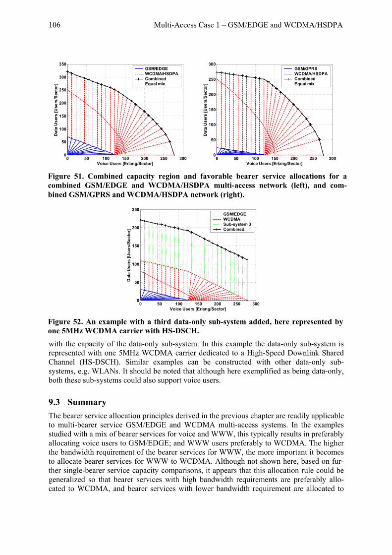
106 Multi-Access Case 1 – GSM/EDGE and WCDMA/HSDPA
with the capacity of the data-only sub-system. In this example the data-only sub-system is represented with one 5MHz WCDMA carrier dedicated to a High-Speed Downlink Shared Channel (HS-DSCH). Similar examples can be constructed with other data-only sub-systems, e.g. WLANs. It should be noted that although here exemplified as being data-only, both these sub-systems could also support voice users.
9.3 Summary The bearer service allocation principles derived in the previous chapter are readily applicable to multi-bearer service GSM/EDGE and WCDMA multi-access systems. In the examples studied with a mix of bearer services for voice and WWW, this typically results in preferably allocating voice users to GSM/EDGE; and WWW users preferably to WCDMA. The higher the bandwidth requirement of the bearer services for WWW, the more important it becomes to allocate bearer services for WWW to WCDMA. Although not shown here, based on fur-ther single-bearer service capacity comparisons, it appears that this allocation rule could be generalized so that bearer services with high bandwidth requirements are preferably allo-cated to WCDMA, and bearer services with lower bandwidth requirement are allocated to
0 50 100 150 200 250 3000
50
100
150
200
250
300
350
Voice Users [Erlang/Sector]
Dat
a U
sers
[Use
rs/S
ecto
r]
GSM/EDGE WCDMA/HSDPACombined Equal mix
0 50 100 150 200 250 3000
50
100
150
200
250
300
Voice Users [Erlang/Sector]
Dat
a U
sers
[Use
rs/S
ecto
r]
GSM/GPRS WCDMA/HSDPACombined Equal mix
Figure 51. Combined capacity region and favorable bearer service allocations for a combined GSM/EDGE and WCDMA/HSDPA multi-access network (left), and com-bined GSM/GPRS and WCDMA/HSDPA network (right).
0 50 100 150 200 250 3000
50
100
150
200
250
Voice Users [Erlang/Sector]
Dat
a U
sers
[Use
rs/S
ecto
r]
GSM/EDGE WCDMA Sub-system 3Combined
Figure 52. An example with a third data-only sub-system added, here represented by one 5MHz WCDMA carrier with HS-DSCH.
Multi-Access Case 1 – GSM/EDGE and WCDMA/HSDPA 107
GSM/EDGE. A capacity gain over allocating bearer services with equal probability in the sub-systems of a factor of 1-2 is achievable. The achievable gain depends on the bearers used in the sub-systems and the bitrate requirements of the bearer service for WWW.


109
Chapter 10 User Assignment in Multi-Access Wireless Networks
As discussed in Section 8.1, in addition to the bearer service type, the actual resource con-sumption of users may also be used as a basis for assigning users to sub-systems. If avail-able, such information may be used to assign users where they are expected to consume the least radio resources, thereby increasing capacity. In addition to assigning users where the resource cost is the smallest, it is as briefly discussed in Section 8.4 desirable to maintain a balanced traffic load between the sub-systems. In this chapter, a set of user assignment algo-rithms is first defined. The set includes algorithms based on bearer service type, radio re-source cost, and combinations thereof. The algorithms further target balanced sub-system loads. Next, expected radio resource costs in different sub-systems, as well as their correla-tion between sub-systems, are discussed. Based on this, the performance of the different al-gorithms is estimated. It should be noted that fairly simple system models are used in this chapter. The results should hence be interpreted as indicating the potential of actual resource cost based user assignment rather than establishing exact performance figures.
10.1 Additional System Models and Selection Variables In order to assign users to the sub-systems in which they in some sense are most efficiently supported, or equivalently consume the least amount of resources, some form of efficiency or cost measure must be defined. Generally applicable such measures are difficult to define. In what follows a simple radio resource cost model with alternative radio resource cost measures and associated capacity measures is presented. The applicability of the model is also discussed.
10.1.1 A Simple Radio Resource Cost Model It is assumed that the total amount of available resources in an access point (covering a cell or a sector) of sub-system m is given by the real-valued scalar wm
tot. The ‘resource cost’ for each user i in sub-system m is given by the real-valued scalar random variable Zm
i. The ran-domness of Zm
i includes effects of e.g. bearer service type, radio environment, and the ap-plied radio resource management solutions. The bearer service type of user i is given by the random variable si. The expected resource cost depends on the bearer service type:
[ ] mni
mi znsZE == (120)
The ‘relative radio resource cost’ for a user of bearer service n in sub-system m is given by:
mtot
mi
mi wZX /= (121)
Xmi thus measures how large fraction of the total available resource is consumed by user i. Its
expectation, the expected relative radio resource cost for a user of bearer service n in sub-system m is given by:
mtot
mn
mn wzx /= (122)
Typically a relationship between the expected relative radio resource cost and the single-bearer service capacity exists so that:

110 User Assignment in Multi-Access Wireless Networks
mn
mtot
mn
msinglen zwxC //1 =≈ (123)
Further, the ‘normalized radio resource cost’ of a user is given by:
ms
mi
mi izZR /= (124)
Rmi thus reflects the amount of resources consumed by user i in sub-system m measured in
‘own-bearer service user-equivalents’. The relationship between the relative radio resource cost and the normalized radio resource cost is given by:
msingles
mi
mtot
ms
mi
mi ii CRwzRX // ≈⋅= (125)
The sub-system assignment of user i is denoted ai. Further, the similar but binary valued variable bi
m is defined as bim = 1 if ai = m, otherwise bi
m = 0.
In the evaluations of this chapter, capacity is measured based on previously determined sin-gle-access capacity limits. It is assumed that acceptable quality is maintained in sub-system m if:
)( mmi
mi
mi CRb αr≤∑ (126)
that is, if the sum of the normalized loads, which corresponds to the total equivalent number of users, does not exceed the capacity for the service mix in question. The combined capac-ity is thus defined as:
∀≤= ∑=
mCRbuC mmu
i
mi
mitot
tot
)(:max)(1
αα rr (127)
As previously seen, the combined capacity depends on which sub-system each user is as-signed to.
In single-bearer service scenarios, using Equation (123) and (124), it may be seen that the condition for acceptable quality in sub-system m in Equation (126) approximately also corre-sponds to m
totimi
mi wZb ≤∑ , which relates the assumed capacity measure to the discussion in
the beginning of this section.
10.1.2 Applicability of the Model First, the above model assumes that the radio resource may be measured as a scalar. Gener-ally this is not the case. However, as discussed in Section 4.1.1, in some special cases it is applicable. Examples of a scalar radio resource include a number of available channels (timeslots, frequencies, spreading codes, etc.), an available downlink power or uplink inter-ference budget.
Further, for the capacity definition in Equation (127) to be valid the resource costs Rim must
be valid at the capacity limit. Generally, the resource costs depend on the number of users in the sub-system and the service mix, i.e. Ri
m = Rim(utot
m, mαr ). Hence, a resource cost meas-ured at a traffic load below the capacity limit is generally not valid at the capacity limit. Such resource costs may thus not be used to estimate the capacity, and may further result in unde-sired user assignments. Therefore, if possible, although measured at lower traffic loads, the resource costs used in the user assignment should preferably reflect the would-be resource cost at the capacity limit. Estimation of such resource costs is not trivial. However, in princi-ple in an interference limited system, a would-be power level could be calculated from users

User Assignment in Multi-Access Wireless Networks 111
pathgains and a known expected interference level at the capacity limit. In cases where the resource costs do not depend on the traffic load, the above is obviously not a problem.
The users assignment algorithms presented in this chapter do not strictly rely on that the re-source costs be valid at the capacity limit. In the special where the relative errors of the esti-mated resources costs are equal for all sub-systems, the user assignment is not affected by the error. However, when the relative errors differ between the sub-systems, undesired user assignments and lower capacity may result.
10.2 Load Balancing As briefly discussed in Section 8.4, in addition to assigning users where the resource cost is the smallest, it is desirable to maintain a balanced traffic load between the sub-systems. The reason for this is twofold. First, an unbalanced traffic load between the sub-systems may yield unnecessarily poor quality for bearer services whose quality depends on the traffic load, e.g. best effort type of bearer services and other bearer services using shared channels.
Secondly, unbalanced traffic loads may reduce capacity in cases where actual resource costs are taken into account in the user assignment, and no user re-assignment may be done. This phenomenon is illustrated for a single-bearer service case in Figure 53, which shows the ag-gregated normalized resource costs as a function of the total number of users. The costs are aggregated both per sub-system and in total. Without load balancing, once sub-system 1 has reached its capacity limit (at about 120 users), no more users can be assigned to it. This means that additional users that enter the system must be assigned to sub-system 2, despite the fact that their cost having been minimized if they were assigned to sub-system 1. The result of this is that the average cost per user increases, which reduces capacity. This effect is indicated in Figure 53 by the increased slope of the total aggregated cost at 120 users.
To achieve a balanced load users should be less likely to be allocated to sub-system 1. This may be realized by rescaling the costs with appropriate factors f1 > 1 in sub-system 1 and f2 <1 in sub-system 2. As a result, the aggregated resource cost is decreased in sub-system 1 and in-creased in sub-system 2. In the example f1 and f2 are selected so that the sub-systems reach their capacity limit for the same total number of users. The benefit of this is that the freedom to select the sub-system for which the resource cost is minimized does not disappear because a sub-system reached its capacity limit, but remains for all traffic loads. In Figure 53
0 50 100 150 2000
20
40
60
80
100
120
Number of Users Utot
Cum
mul
ativ
e N
orm
aliz
ed C
ost
No load balancingLoad balancing
Sub-system 1
Sub-system 2
Sub-system 1 +Sub-system 2
Σ R2i max
Σ R1i max
Cunbal Cbal
Figure 53. Load balancing may increase capacity.

112 User Assignment in Multi-Access Wireless Networks
this is reflected by there being no sudden increase in the slope of the total aggregate resource cost curve in the balanced case The drawback is that the rule of assigning users where the resource cost is smallest is compromised; some users are assigned in a sub-system where the cost is slightly higher than in other sub-systems. This can be seen by the slight increase in the total aggregate resource cost curve in the balanced case. Overall however, the effect is positive, the capacity increases from Cunbal ≈ 160 to Cbal ≈ 180.
Unfortunately, selection of the scaling cost factor fm is typically not trivial. The appropriate value of fm depends on the sub-system capacities )( mmC αr and the resource cost distribu-tions, which in turn also may depend on the service mix αr , hence )),(( αα rr mm
mm Cff = . A rescaling of the resource costs may further affect the sub-system service mixes mαr , which further complicates finding appropriate values. In this study appropriate values of fm are typically derived empirically. However, in some special cases it is possible to estimate ap-propriate values analytically.
An alternative way to avoid capacity reductions when one sub-system becomes full before the others is through reassignment of users. Assuming that a gain for assigning each user to its best sub-system over assigning it to other sub-systems can be determined, this can be done by assigning new users to the already full sub-system if the associated gain is larger than that of some of the already assigned users, who are then reassigned to its next best sub-system. It is also required that the absolute cost in the full sub-system is not increased by the reallocation. This way sub-systems are assigned the set of users for which the gain is the largest.
More formally, with two sub-systems 1 and 2, and a user A assigned to the full sub-system 1 when user B arrives, user B is assigned to sub-system 1 and user B is reassigned to sub-system 2 if:
111212 & ABAABB CostCostCostCostCostCost <−>− (128)
where the cost measures Costim are defined according to the desired selection variable, see
Section 10.1 and Section 10.3 for alternatives.
10.3 User Assignment Algorithms This section proposes a set of different user assignment algorithms. The algorithms are straightforwardly developed with the different cost measures of Section 10.1 as decision variables. The intention is mainly to indicate what results may be expected for different deci-sion variables. Although it is not obvious, better assignment algorithms may well be found. For each algorithm, an expression for the sub-system assignment ai is first given when disre-garding load balancing aspects, then it is discussed how the algorithms may be modified to take load balancing into account.
10.3.1 Algorithm 1: Random Assignment
The simplest user assignment algorithm does not take into account bearer service type or ra-dio resource costs. Disregarding load balancing, the assignment of users may be done ran-domly with probabilities:
MmaP i /1)( == (129)
This user assignment principle typically results in unbalanced loads, since sub-systems with low capacities are likely to be filled before sub-systems with high capacities. To balance

User Assignment in Multi-Access Wireless Networks 113
loads, the probability of assigning a user to a sub-system can be set equal to the sub-system’s normalized capacity. The normalized capacity of sub-system m is defined as:
∑
=
= M
k
k
mmnorm
C
CC
1
)(
)()(
α
αα
r
rr (130)
Note that the normalized capacities depend on the service mix. To balance the sub-system loads, for a service mix αr , the user assignment should be done with probabilities:
)()( αrmnormi CmaP == (131)
Generating a random variable with this distribution can be done using standard methods. Re-gardless of whether load balancing is taken into account or not, this assignment principle re-sults in equal expected service mixes and unbiased radio resource cost distributions in all sub-systems.
10.3.2 Algorithm 2: Bearer Service-Based Assignment A bearer service-based assignment algorithm may be realized by assigning users in the sub-system where their expected relative radio resource cost for the bearer service type in ques-tion is the smallest. User assignment may hence be done according to:
{ }msmi ixa minarg= (132)
Provided that all sub-systems have linear capacity regions, this assignment rule will, when all sub-systems have been filled, result in a user assignment such that:
)()( * αβ rmni maP == (133)
where )(* αβ rmn is the near-optimum relative sub-system bearer service allocations derived in
Chapter 8. Under such conditions, provided that the bearer service type is the only available decision variable, this user assignment algorithm may be considered to yield near optimum combined capacity.
The assignment rule of Equation (132) may result in severely unbalanced traffic loads be-tween sub-systems, as all users of a certain bearer service are allocated to a single sub-system until that sub-system is full. To balance loads between sub-systems, ai can be gener-ated directly from a distribution based on Equation (133).
10.3.3 Algorithm 3: Normalized Radio Resource Cost-Based Assignment The bearer service-based assignment algorithm assigns users in the sub-system where the expected radio resource cost is the smallest. It may happen that the actual radio resource cost is the smallest in a sub-system different from the one where the expected cost is the smallest. Such effects are not captured by the bearer service-based assignment rule. A straightforward user assignment algorithm based on actual radio resource cost may be realized by assigning users where the normalized radio resource cost is the smallest. In this case, ai is defined as follows:
{ }mimi Ra minarg= (134)
As with the random assignment rule defined in Section 10.3.1, the above rule results in un-balanced traffic loads, since sub-systems with low capacities are filled before sub-systems with large capacities. To achieve balanced sub-system loads, the normalized resource costs

114 User Assignment in Multi-Access Wireless Networks
in systems with low capacities may be scaled up by a factor fm so that only users that have significantly lower resource costs in those systems are assigned to them. Appropriate values of fm have been empirically derived, and are plotted in Figure 54.
10.3.4 Algorithm 4: Relative Radio Resource Cost-Based Assignment An alternative to assigning users in the sub-system where the normalized radio resource cost is minimized is to assign them where the relative resource cost is minimized. In this case the definition of ai becomes:
{ }mimi Xa minarg= (135)
In contrast to assigning users where the normalized radio resource cost is minimized, this assignment rule also takes into account the fact that bearer services are supported more or less well in different sub-systems. This however also results in users sometimes being as-signed to sub-systems in which the cost measured in user equivalents is not minimized.
Using the algorithm stated in Equation (135) typically results in unbalanced sub-system loads. Cost scaling factors that yield balanced loads are plotted in Figure 54. These have been derived empirically.
10.3.5 Algorithm 5: Equivalent Normalized Radio Resource Cost-Based Assignment
A drawback of the above actual radio resource cost based assignment algorithm is that it does not take into account the capabilities of the sub-systems to handle different bearer ser-vices. As previously discussed, the relationship between the expected radio resource costs for different bearer services may differ between the sub-systems. Consequently, it may hap-pen that although the normalized radio resource cost for a particular user is the lowest in one sub-system, the expected number of users of other bearer services that could have been as-signed using that resource is still higher than in other sub-systems. To take this phenomenon into account, the radio resource cost should preferably be measured not only in units of user equivalents of their own bearer service type, but in user equivalents across all bearer service types. The following definition of ai takes this into account:
0 0.2 0.4 0.6 0.8 10
0.5
1
1.5
Fraction of Voice Users α v
Cos
t Inc
reas
e Fa
ctor
in S
ub-S
yste
m 1
(f1)
Alg 3, ρ=0.5Alg 3, ρ=0.7Alg 4, ρ=0.5Alg 4, ρ=0.7Alg 5, ρ=0.5Alg 5, ρ=0.7
Figure 54. Radio resource cost rescaling factor in sub-system 1 (f1) as a function of the fraction of voice users for algorithms 3, 4, and 5. The resource costs in sub-system 2 are not rescaled, i.e. f2=1.

User Assignment in Multi-Access Wireless Networks 115
ms
mnm
n
N
n
mn
minmi
iCC
kkRasingle
single
1;minarg =
⋅⋅= ∑=
α (136)
For each bearer service, the normalized radio resource cost is thus weighted by both the frac-tion of users of the bearer service in question αn, as well as with the relationship between the single-bearer service capacity for this bearer service and their own-bearer service kn
m, and finally summed over the bearer services to form the decision variable. As a result, the cost is scaled down in sub-systems where the capacity in comparison to other bearer services is relatively high, and scaled up in sub-systems where the capacity is relatively low.
Despite containing elements of load balancing, this assignment rule may also result in unbal-anced sub-system loads. To mitigate against this, the decision variables may be scaled up in sub-systems with low capacities. As for the other actual cost-based assignment rules, these factors have been derived empirically and are plotted in Figure 54.
10.3.6 Algorithm 6: Most Resources Left An alternative to assigning a user where its resource consumption is the smallest is to assign it in the sub-system that, after the assignment, would have the most resources left. This as-signment rule may be formulated as:
{ } ∑=
=−−=curu
j
mj
mj
mcur
mi
mcurmi XbXXXa
1;1maxarg (137)
where ucur is the current number of users in the system. This assignment rule inherently re-sults in balanced sub-system load. The drawback is that users are not necessarily assigned to the sub-systems where their resource cost is minimized.
10.4 Expected Radio Resource Costs The statistical properties of the radio resource costs in the sub-systems have a significant ef-fect on the performance of the user assignment algorithms taking the actual radio resource cost into account. Both the distribution of the radio resource cost within each sub-system, and the correlation of the costs between sub-systems matter. These further depend on the characteristics of the sub-systems, e.g. whether they are blocking or interference limited, whether the access points are co-located, etc. It is hence difficult to make any generally ap-plicable assumptions. The approach taken here is to evaluate the user assignment algorithms for one measurement and simulation based snapshot of cost distributions and correlations for combined GSM/EDGE and WCDMA systems. Some of the parameters are varied to verify the behavior of the algorithms under different conditions.
Measurements and simulations of GSM/EDGE and WCDMA systems14 indicate that at the capacity limit, the downlink power consumption, which is the limiting factor, may be ap-proximated by a truncated lognormal distribution with a standard deviation of 6dB. This dis-tribution function is depicted in the left graph in Figure 55. Further, by twisting the sector antennas for the different sub-systems so that the sectors point in different directions, the correlation of the pathloss ρ, which may be used to approximate the required downlink
14 These measurements and simulations have been provided by Mr. Arne Simonsson at Ericsson Research, and are not a contribution of the dissertation author.

116 User Assignment in Multi-Access Wireless Networks
power, may be reduced from 1.0 to approximately 0.5 to 0.7 depending on propagation char-acteristics. A scatter plot of the radio resource costs for the case of a correlation of 0.7 is shown in the right graph in Figure 55.
10.5 Evaluation Methodology To evaluate the performance of the different user assignment algorithms, simple simulations with two bearer services and two sub-systems are run. Normalized radio resource costs for a number of users are randomly generated according to the statistical properties described in Section 10.4. Sub-system capacity regions for GSM/EDGE and WCDMA mixed voice and WWW traffic are assumed (see Figure 48 left). The single bearer service capacities of these sub-systems are used to transform normalized relative radio resource costs to relative radio resource costs using Equation (125).
If no user reassignments are done, users are sequentially assigned a sub-system according to the assignment algorithm in question until one of the sub-systems is fully loaded. Following this users are only assigned to the non-full sub-system until that sub-system also is full. When the versions of the assignment algorithms taking load balancing into account are used, the resource costs are multiplied with appropriate factors f1 and f2 in sub-system 1 and 2 re-spectively as discussed in Section 10.2. If user reassignment is used, according to Equation (128), users may be reassigned from their initial sub-system if new users, for which the gain is larger, enter the system. The full range of service mixes is covered. For each service mix the simulation is repeated 16 times to improve the reliability of the results. The overall ca-pacity is measured according to Equation (127). It is assumed that radio resource costs that are valid at the capacity limit are available regardless of the actual traffic load.
10.6 Numerical Results This section presents simulated capacity regions for the different assignment algorithms. Re-sults are presented first without both load balancing and user reassignment, then with load balancing but no reassignment, and finally with reassignment but no load balancing. The case with both load balancing and reassignment is not included since with load balancing
-15 -10 -5 0 5 100
10
20
30
40
50
60
70
80
90
100
C.D
.F.
[%]
Normalized Cost in Sub-system 1 [dB]-10 -5 0 5
-12
-10
-8
-6
-4
-2
0
2
4
6
Normalized Cost in Sub-system 1 [dB]
Nor
mal
ized
Cos
t in
Sub-
syst
em 2
[dB
]
Figure 55. Distribution of normalized radio resource costs (left) and scatter plot of ra-dio resource costs in different sub-systems for ρ = 0.7 (right).

User Assignment in Multi-Access Wireless Networks 117
user reassignment is not necessary. Further, scenarios with cost correlations of both 0.7 and 0.5 are covered.
10.6.1 No Load Balancing, no User Reassignment
Simulated capacity regions for the different assignment algorithms without load balancing and user reassignment are shown in Figure 56. The left graph shows the results achieved with a radio resource cost correlation of 0.7 and the right graph results achieved with a corre-lation of 0.5. It is seen that the performance of the assignment algorithms improves with the level of detail in the radio resource cost measure. The relationship between the random and bearer service-based assignment algorithms is as expected as previously seen in Figure 48 in Chapter 8. The achievable capacities for these assignment algorithms are further independent of the correlation of the radio resource costs, which is natural since these are not taken into account in the assignment.
Taking the actual radio resource cost into account is seen to improve capacity. The gain is larger in the scenario with lower cost correlation. The highest capacity is achieved with algo-rithm 6 that uses equivalent normalized resource costs. Algorithms 3, 4, and 5 perform ap-proximately equally well. Note also that for all actual cost-based algorithms apart from algo-rithm 6, the gain is smaller the higher the fraction of data users. This depends on unbalanced loads between the sub-systems, as discussed in Section 10.2 (in fact, the load balancing ex-ample in Figure 53 is for algorithm 3 with only data users). For data bearer services sub-system 2 has significantly higher capacity than sub-system 1. Sub-system 1 thus typically becomes full before sub-system 2 and the flexibility to select sub-systems is lost. For voice the capacities are similar, and the sub-system loads are closer to balanced. For algorithm 6, which inherently balances the sub-system load, the gain is more consistent.
10.6.2 Load Balancing
Figure 57 shows the capacity regions achieved with load balancing. This does not affect the capacities for algorithms 1 and 2 since they do not take actual costs into account. Nor is the capacity achieved with algorithm 6 affected, since it is inherently load balanced. For the other algorithms however a significant improvement is achieved, especially for high frac-tions of data users.
0 50 100 150 200 250 300 350 4000
20
40
60
80
100
120
140
Voice Users
Dat
a U
sers
1: Random 2: Service 3: Normalized 4: Relative 5: Eq. Normalized6: Rem. Relative
0 100 200 300 400 5000
20
40
60
80
100
120
140
160
Voice Users
Dat
a U
sers
1: Random 2: Service 3: Normalized 4: Relative 5: Eq. Normalized6: Rem. Relative
Figure 56. Combined capacity regions for the different user assignment principles with-out load balancing. The gain for taking actual cost into account is larger with low cost correlation between the systems (left).

118 User Assignment in Multi-Access Wireless Networks
Assigning users where the normalized radio resource cost is minimized, i.e. algorithm 3, now yields a rather constant capacity gain over random user assignment. This gain is ap-proximately inversely proportional to the expected reduction in radio resource cost, i.e. E[Rm
i] / E[min{R1i, R2
i}]. With a radio resource cost correlation of 0.7, a gain in the order of 35% is achieved, whereas with a correlation of 0.5 the gain reaches about 55%. A small ad-ditional capacity gain for mixed bearer services is enabled by the relative or equivalent nor-malized radio resource cost-based algorithms, whose performance is close to identical. For a radio resource cost correlation of 0.7, an additional capacity gain of up to 12% is enabled. This gain decreases as the correlation decreases. This occurs because when the radio re-source costs vary more between the sub-systems, the relative importance of taking this into account increases as compared to taking the sub-system capacities into account. Also note that the gains achieved with bearer service-based and normalized cost-based assignment are not additive. The reason for this is that a part of the cost difference is already taken into ac-count by the bearer service type.
10.6.3 User Reassignment
In Figure 58 the capacity regions achieved with user reassignment are shown. The results are very close to those previously achieved with load balancing. In terms of capacity these solu-tions are thus equally good. However, load balancing also maintains a balanced load be-tween the sub-systems for traffic loads below the capacity limit, which may be desired. Im-plementation aspects also differ between the approaches. Load balancing requires empirical estimation of appropriate cost factors, whereas user reassignment requires more frequent re-assignment of users between sub-systems. Note that in practice reassignments are also nec-essary with load balancing to track resource costs that typically vary over time.
10.6.4 Resulting User Assignments per Bearer Service In Figure 59, the combined capacity regions with load balancing for a cost correlation of 0.7 are plotted in different graphs, including vectors indicating the assignment of users in the sub-systems are also included. Similar results are achieved with user reassignment. It is seen that for the bearer service-based assignment algorithm (upper right plot), the user assignment is as expected equal to that of Figure 48. For the random (upper left plot) and normalized (middle left plot) cost-based assignment algorithms, the service mix is equal in both sub-
0 50 100 150 200 250 300 350 4000
20
40
60
80
100
120
140
Voice Users
Dat
a U
sers
1: Random 2: Service 3: Normalized 4: Relative 5: Eq. Normalized6: Rem. Relative
0 100 200 300 400 5000
20
40
60
80
100
120
140
160
180
Voice Users
Dat
a U
sers
1: Random 2: Service 3: Normalized 4: Relative 5: Eq. Normalized6: Rem. Relative
Figure 57. Combined capacity regions for the different user assignment principles with load balancing. The gain for taking actual cost into account is larger with low cost cor-relation between the systems (left).

User Assignment in Multi-Access Wireless Networks 119
systems, whereas for the relative and equivalent normalized cost-based assignment (middle right and lower left plots) the service mixes are a compromise between what is achieved with bearer service-based and normalized cost based assignment. The reason for this is that the actual resource cost sometimes is lower in the sub-system where its expectation conditioned on the bearer service type is higher. The same reasoning also applies to the most relative re-sources left-based assignment algorithm (lower right plot), which however yields more simi-lar service mixes.
10.6.5 The Impact of Cost-Estimate Errors
The resource cost-based assignment algorithms rely on accurate and frequent estimation of the resource costs. In the previous analyses resource costs have been assumed to be without errors and instantly available. In practice the estimates will have measurement errors and be delayed. To investigate the impact of this an error is added to the resource cost before using it for user assignment. The error is assumed to be independent between the sub-systems and log-normally distributed. The standard deviation is varied between 0.5 and 6dB.
Figure 60 shows the capacity regions achieved with the equivalent normalized cost based assignments algorithm (algorithm 5) for different measurement errors. The capacity regions achieved with random and bearer service-based assignment are also shown. Cost correlations of 0.7 and 0.5 are used in the left and right plots respectively. It is seen that the achievable capacity reduces rapidly with the measurement error. Already for a measurement error of 2dB the bearer service based assignment algorithm yields better results than algorithm 5 for some service mixes. For larger errors the performance approaches that of random assign-ment. This might be expected since the cost estimates are so unreliable that the assignment becomes close to random. Similar results may be derived for the other actual cost-based as-signment algorithms.
10.7 Summary The bearer service type of a user reflects an expected radio resource cost in each sub-system. The actual radio resource cost may differ from its expectation. By taking this into account when assigning users to sub-systems, further capacity gains are achievable. The achievable gain depends on the distributions and correlation of the radio resource costs between the sub-
0 50 100 150 200 250 300 350 4000
20
40
60
80
100
120
140
Voice Users
Dat
a U
sers
1: Random 2: Service 3: Normalized 4: Relative 5: Eq. Normalized6: Rem. Relative
0 100 200 300 400 5000
20
40
60
80
100
120
140
160
180
Voice Users
Dat
a U
sers
1: Random 2: Service 3: Normalized 4: Relative 5: Eq. Normalized6: Rem. Relative
Figure 58. Combined capacity regions for the different user assignment principles with user reassignment. The results are very similar to those with load balancing.

120 User Assignment in Multi-Access Wireless Networks
systems. To fully exploit the achievable gain, load balancing or user reassignment is further seen to be required, as well as accurate estimates of the resource costs.
In an example that aims to reflect a multi-access GSM/EDGE and WCDMA system, capac-ity gains in the order of 50% are achievable. It should be noted that user assignment based on the actual radio resource cost is more complex than bearer service-based user assignment. The actual radio resource cost varies in time, and needs to be tracked and users reassigned for to maintain the capacity gain.
0 50 100 150 200 250 3000
20
40
60
80
100
120
Voice Users
Dat
a U
sers
Combined CapacitySubsystem 1 Subsystem 2
0 50 100 150 200 250 3000
20
40
60
80
100
120
Voice Users
Dat
a U
sers
Combined CapacitySubsystem 1 Subsystem 2
0 50 100 150 200 250 300 350 4000
20
40
60
80
100
120
140
160
Voice Users
Dat
a U
sers
Combined CapacitySubsystem 1 Subsystem 2
0 50 100 150 200 250 300 350 4000
20
40
60
80
100
120
140
160
Voice Users
Dat
a U
sers
Combined CapacitySubsystem 1 Subsystem 2
0 50 100 150 200 250 300 350 4000
20
40
60
80
100
120
140
160
Voice Users
Dat
a U
sers
Combined CapacitySubsystem 1 Subsystem 2
0 50 100 150 200 250 300 3500
20
40
60
80
100
120
140
Voice Users
Dat
a U
sers
Combined CapacitySubsystem 1 Subsystem 2
Figure 59. Simulated capacity regions and 95% confidence intervals for assignment al-gorithms 1 – 6 (1 2; 3 4; 5 6) with load balancing. The resource cost correlation is 0.7.

User Assignment in Multi-Access Wireless Networks 121
0 50 100 150 200 250 300 350 4000
50
100
150
Voice Users
Dat
a U
sers
Alg. 5 0dB Alg. 5 0.5dBAlg. 5 1dB Alg. 5 2dB Alg. 5 6dB Service Random
0 100 200 300 400 5000
20
40
60
80
100
120
140
160
180
Voice Users
Dat
a U
sers
Alg. 5 0dB Alg. 5 0.5dBAlg. 5 1dB Alg. 5 2dB Alg. 5 6dB Service Random
Figure 60. Combined capacity regions for assignment algorithm 8 for different meas-urement errors, in comparison with random and bearer service-based assignment. Left: ρ = 0.7. Right: ρ = 0.5.


123
Chapter 11 Conclusions In summary, the results of this dissertation indicate that by employing the proposed interfer-ence balancing principle, multiple bearer services may efficiently coexist within one radio access technology. Further, with the possibility to use multiple radio access technologies, for a given service mix combined capacities beyond the sum of the sub-system capacities may be achieved by using simple bearer service allocation principles that allocate bearer services to the sub-system relatively best at supporting them. In what follows the conclusions of the dissertation are discussed in greater detail.
11.1 How to Share Resources between Bearer Services? Per-service capacity balancing is a necessary requirement for maximizing capacity in multi-ple bearer service cellular systems. In interference-limited scenarios per-service capacity balancing can be accomplished by interference balancing, i.e. allocating radio resources so that the maximum interference levels tolerated are equal for all bearer services. Interference balancing can further be realized by adjusting the maximum output power per individual bearer for each bearer service. A benefit of this solution is that it does not statically allocate a fixed power budget per bearer service group, which might result in performance losses, but instead flexibly follows variations in the service mix.
In scenarios where the maximum tolerable interference level and the interference contribu-tions per user are independent of the service mix, interference balancing results in a capacity region delimited by a straight-line between the single-bearer service capacity endpoints. This might be interpreted as the single-bearer service capacities being preserved in a relative sense; removing a certain fraction of users for one bearer service leaves room for the same fraction of users of other bearer services. If interference balancing cannot be achieved, the loss in capacity is given by the traffic load loss associated with the difference in maximum interference levels between the bearer services. This loss is typically lower for power-controlled bearer services for which the interference level to traffic load characteristics are steeper than for non-power controlled bearer services.
In scenarios where the interference tolerance depends on the service mix, service mix-dependent interference balancing is required to maximize capacity. The resulting perform-ance depends on whether the tolerable interference levels from other bearer services are higher or lower than the tolerable own-interference. In the former case, convex capacity re-gions are achieved, whereas the latter case yields concave capacity regions. An example of the former case is a system where one bearer service is partially blocking limited.
A set of case studies indicates that the interference balancing principles may straightfor-wardly be used to maximize capacity in GSM/EDGE and WCDMA systems. The resulting capacity regions may further be explained by simple theoretical expressions. For GSM/EDGE, linear capacity regions are achieved in interference limited scenarios. This is also approximately valid when data performance is limited by queuing in addition to inter-ference. In scenarios with blocking limited voice bearers on the other hand, convex capacity regions appear. This is due to a higher interference tolerance for voice bearers for service mixes with smaller fractions of voice users, for which less blocking occurs. The capacity gain achievable with interference balancing varies with the interference tolerance levels of

124 Conclusions
the bearer services before interference balancing. Capacity gains of up to 50% are seen in the examples studied.
Also, for SIR-balancing power controlled bearers in WCDMA linear capacity regions are achieved. The achievable capacity gain grows with the difference in SIR target of the bear-ers. For SIR target differences of 3-10dB, capacity gains in the order of 10-25% are achiev-able respectively. Interference balancing may also be used in scenarios including the WCDMA HS-DSCH. With sufficiently high maximum power for voice bearers, the system is inherently close to balanced, and small additional gains may be achieved. In this case con-vex capacity regions appear. This is due to the fact that voice bearers tolerate more interfer-ence the fewer voice bearers there are.
11.2 How to Allocate Bearer Services onto Sub-Systems? The capability to handle bearer services typically differs between radio access technologies. Therefore, the allocation of bearer services on to sub-systems in multi-access systems affects the overall capacity. Favorable, near-optimum, sub-system bearer service allocations may be found using a straightforward maximization procedure. These favorable bearer service allo-cations are either characterized by the relative efficiency of supporting bearer services being equal in all sub-systems, or they are extremes where bearer services are isolated in different sub-systems. The former solution typically appears with linear or concave sub-system capac-ity regions. Bearer services should in this case as far as possible be allocated to the sub-system relatively best at supporting them. The latter solution typically requires at least one convex sub-system capacity region. In this case, bearer services should be mixed in the sub-systems so that the relative efficiency of supporting bearer services is kept equal. The capac-ity gain achievable by employing the proposed bearer service allocation strategy depends on the individual sub-system capacity region characteristics. Roughly speaking, the more differ-ent capacity regions, the higher the possible gains.
The above bearer service allocation principles are readily applicable to multi-bearer service GSM/EDGE and WCDMA multi-access systems. The resulting bearer service allocations typically involve preferably allocating bearer services with moderate bandwidth require-ments to GSM/EDGE, and bearer services with higher bandwidth requirements preferably to WCDMA. In the examples studied, these are represented by bearer services for voice and WWW respectively. The achievable capacity compared to the reference case of allocating bearer services with equal probability in the sub-systems gain depends on the bearer realiza-tions used in the sub-systems and the bitrate requirements of the bearer service for WWW. Capacity gains of a factor of 1-2 are achieved in the studied examples.
The bearer service type of a user may be considered to reflect an expected radio resource cost in each sub-system. The actual radio resource cost may differ from its expectation. Fur-ther capacity gains are achievable by taking this into account when assigning users to sub-systems. The achievable gain depends on the distributions and correlation of the radio re-source costs between the sub-systems. To fully exploit the achievable gain, accurate esti-mates of the resource costs as well as either load balancing or user reassignment is required. In an example attempted to reflect a multi-access GSM/EDGE and WCDMA system, capac-ity gains of up to 50% are reached.
It may further be noted that the proposed bearer service allocation principles are not strictly limited to multi-access systems. Similar rules apply also to single-access systems where the

Conclusions 125
resource somehow is divided into different pools, e.g. multi-carrier DS-CDMA systems, sys-tems with micro and macro layers, etc.
11.3 Further Studies Throughout this work, the goal has been to maximize the capacity, measured in the number of supported users, for a given service mix. This also maximizes the revenue generated by the system for that service mix, under the assumption that the revenue per bearer service grows with the number of users of the bearer service. However, if the service mix can be controlled, larger revenues may be achieved, possibly through using other resource sharing and bearer service allocation principles.
The resource sharing and bearer service allocations principles proposed in this dissertation were further developed largely neglecting dynamics in radio and traffic conditions. The in-terference contribution per user is for example represented by its expected value. Consider-ing such dynamics may yield better results. An indication of this is seen in Chapter 10, where higher capacities are achieved when actual rather than expected radio resource costs are used as a basis for user assignment.
Regarding the multi-bearer service case studies, these could be extended to further verify the theoretical principles of Chapter 4. More bearer services than those studied could of course be included, e.g. bearer services for conversational video, streaming, or background data transfer. It may be expected that similar results will be achieved if bearer realizations resem-bling those used for voice or WWW in this work are used, but this remains to be verified. Including higher layer protocol aspects, foremost including TCP effects for WWW, is also of great interest.
The multi-access principles are developed under the assumption that different sub-systems are run by one single operator or a set of cooperating operators. Principles to use in multi operator scenarios also should be developed. As regards the user assignment principles pro-posed in Chapter 10, the principles based on actual radio resource costs are initial attempts, mainly intended to show that better performance than what is achieved with bearer service-based allocation can be achieved when more information is available. It is probably possible to find assignment rules that provide yet better results. In the multi-access case studies, sub-systems of WLAN type, e.g. IEEE802.11b/a, or of broadcast type, e.g. DAB or DVB, could be included. Another aspect overlooked in development of the bearer service allocation and user assignment is the existence of single-mode terminals.


127
References [1] Strategy Analytics, “Worldwide Cellular Forecast Update (2001 - 2006)”, available at
www.strategyanalytics.com/cgi-bin/greports.cgi?rid=162001080611 (accessed 2003-03-21).
[2] Ovum, “Cellular Connections - World”, mobile@ovum, December 2002.
[3] E. Gustafsson and A. Jonsson, “Always Best Connected”, in IEEE Wireless Communi-cations Magazine, pp. 49-55, Volume 10, Issue 1, February 2003.
[4] 3rd Generation Partnership Project, “Quality of Service Concept and Architecture”, TS 23.107, v. 3.5.0, 2000-12, available at www.3gpp.org/ftp/Specs/archive/23_series/ 23.107/ (accessed 2003-03-21).
[5] ITU, “Performance and Quality of Service Requirements for International Mobile Telecommunications-2000 (IMT-2000)”, Recommendation ITU-R M.1079-1.
[6] D. J. Goodman, R. A. Valenzuela, K. T. Gayliard and B. Ramamurthi, “Packet Reser-vation Multiple Access for Local Wireless Communications”, in IEEE Transactions on Communications, pp. 885 -890, Vol. 37, No. 8, August 1989.
[7] N. Guo and S. D. Morgera, “The Grade of Service for Integrated Voice/Data DS-CDMA Networks”, in proceedings of the IEEE International Conference on Commu-nications 1994(ICC’94), pp. 1104-1110, vol. 2, May 1994.
[8] A Sampath, P. S. Kumar and J. M. Holtzman, “Power Control and Resource Manage-ment for a Multimedia CDMA Wireless System”, in proceedings of IEEE Personal, Indoor Mobile Radio Conference 1995 (PIMRC’95), pp. 21-25, Vol. 1, September 1995.
[9] A Sampath, N. B. Mandayam and J. M. Holtzman, “Erlang Capacity of a Power Con-trolled Voice and Data CDMA System”, in proceedings of IEEE Vehicular Technology Conference 1997 (VTC’97), pp. 1557-1561, Vol. 3, May 1997.
[10] N. B. Mandayam, J. Holtzman and S. Barberis, “Erlang Capacity for an Integrated Voice/Data DS-CDMA Wireless System with Variable Bit Rate Sources”, in proceed-ings of the IEEE Personal, Indoor Mobile Radio Conference 1995 (PIMRC’95), pp. 1078-1082, Vol. 3, September 1995.
[11] S. J. Lee and D. K. Sung, “Capacity Evaluation for DS-CDMA Systems with Multi-Class On/Off Traffic”, in IEEE Communications Letters, pp. 153-155, Vol.2, No.6 June 1998.
[12] M. K. Park and S. K. Oh, “Power Allocation and Capacity Analysis in Multi-Class DS-CDMA Systems with Power Control Error”, in proceedings of the IEEE Interna-tional Conference on Communications 2001(ICC’2001), pp. 2943-2947, Volume 9, June 2001.
[13] I. Koo, J. Yang, Y. Choi and K. Kim, “Capacity-Optimised Power allocation Scheme in an Integrated Voice and Data DS-CDMA System”, in proceedings of IEEE Region 10 Conference 1999 (TENCON’99), pp. 1178-1181, Vol. 2, December 1999.

128 References
[14] J. B. Kim and M. L. Honig, “Resource Allocation for Multiple Classes of DS-CDMA Traffic”, in IEEE Transactions on Vehicular Technology, pp. 506-519, Vol. 49, No. 2, March 2000.
[15] J. H. Kim, T. S. Kim, Y. W. Kim and D. S. Sung, “Hybrid Channel Assignment Scheme for Accommodating Voice/Data Traffic in DS-CDMA Cellular Systems”, in IEEE Transactions on Vehicular Technology, pp. 1566-1577, Vol. 49, No. 5, Septem-ber 2000.
[16] D. Ayyagari and A Ephrimides, “Cellular Multicode CDMA Capacity for Integrated (Voice and Data Services)”, in IEEE Journal on Selected Areas in Communications, pp. 928-938, Vol. 17, No. 5, May 1999.
[17] H. Azad, A. H. Aghvami and W. C. Chambers, “Multiservice / Multirate Pure CDMA for Mobile Communications”, in IEEE Transactions on Vehicular Technology, pp. 1404-1413, Vol. 48, No. 5, September 1999.
[18] L. Wang and H. A. Aghvami, “Optimal Power Allocation Based on QoS Balance for a Multi-rate Packet CDMA System with Multi-media Traffic”, in proceedings of the IEEE Global Telecommunications Conference – Globecom’99, pp. 2778-2782, vol. 5, May 1999.
[19] L. Wang and H. A. Aghvami, “Optimal Power Allocation for a Multi-rate Packet CDMA System with Multi-media Traffic”, in proceedings of the IEEE WCNC’99, pp. 119-123, vol. 5, September 1999.
[20] Q. Zhang, “UMTS Air Interface Voice/Data Capacity – Part 2: Forward Link Analy-sis”, in proceedings of the IEEE Vehicular Technology Conference 2001 spring, (VTC’01 spring), pp. 2730-2734, Vol. 4, May 2001.
[21] W. Choi and J. Y. Kim, “Forward Link Capacity of 3G Wideband CDMA System with Mixed Traffic Sources”, in proceedings of the IEEE Vehicular Technology Conference 2001 spring (VTC’01 spring), pp. 2620-2624, Vol. 4, May 2001.
[22] G. Bianchi et al., “Packet Data Services over GSM Networks with Dynamic Stealing of Voice Channels”, in proceedings of the IEEE Global Telecommunications Confer-ence1995 (Globecom’95), pp. 1152-1156, vol. 2, November 1995.
[23] S. Ni, Y. Liang and S-G Häggman, “Outage Probability for GPRS over GSM Voice Services”, in proceedings of IEEE Vehicular Technology Conference 1999 Fall (VTC’99 fall), pp. 839-843, Vol. 2, September 1999.
[24] J. M. Jacobsmeyer, “Capacity of Channel Hopping Channel Stream On Cellular Digi-tal Packet Data (CDPD)”, in proceedings of IEEE Vehicular Technology Conference 1995 (VTC’95), pp. 346-350, Vol. 1, July 1995.
[25] S. Ni, and S-G Häggman, “GPRS performance estimation in GSM circuit switched services and GPRS shared resource systems”, in proceedings of IEEE Wireless Com-munications and Networking Conference 1999 (WCNC’99), pp. 1417-1421, vol. 3, September 1999.
[26] P. Stuckmann et al., “GPRS radio Network Capacity and Quality of Service using Fixed and On-Demand Channel Allocation Techniques”, in proceedings of IEEE Ve-hicular Technology Conference 2000 spring (VTC’2000 spring), pp. 440-444, Vol. 1, May 2000.
References 129
[27] M Mahdavi and R. Tafazolli, “Analysis of Voice and Data for GPRS”, in proceedings of IEE First International Conference on 3G Mobile Communication Technologies, pp. 436-440, March 2000.
[28] R. Rodriguez, J. Martinez and J. Romero, "Downlink Power Control Performance in (E)GPRS Networks", in proceedings of the IEEE Vehicular Technology Conference, 2002 fall (VTC’2002 fall), pp. 1125-1128, Vol. 2, September 2002.
[29] M. Salmenkaita, J. Gimenez, P. Tapia and M. Fernandez-Navarro, “Optimizing the GSM/EDGE air interface for multiple services with dynamic frequency and channel assignment”, in proceedings of the IEEE Vehicular Technology Conference, 2002. Proceedings (VTC’2002 fall), pp 2215-2219, Vol. 4, September 2002.
[30] J. Gimenez, P. Tapia, M. Salmenkaita, and M. Femandez-Navarro, "Analysis of Dy-namic Frequency and Channel Assignment in Irregular Network Environment", in pro-ceedings of the 5th International Symposium on Wireless Personal Multimedia Com-munications (WPMC’2002), pp. 863-867, Vol. 2, October 2002.
[31] R. De Bernardi et al., “Load Control Strategies for Mixed Services in WCDMA”, in proceedings of IEEE Vehicular Technology Conference 2000 Spring (VTC’2000 spring), pp. 825-829, Vol. 2, May 2000.
[32] D. Imbeni and M. Karlsson, “Quality of Service Management for Mixed Services in WCDMA”, in proceedings of IEEE Vehicular Technology Conference 2000 Fall (VTC’2000 fall), pp. 565-572, Vol. 2, September 2000.
[33] Q. Zhang and O. N. Yue, “UMTS Air Interface Voice/Data Capacity – Part 1: Reverse Link Analysis”, in proceedings of the IEEE Vehicular Technology Conference 2001 spring (VTC’01 spring), pp. 2725-2729, May 2001.
[34] J. Y. Song and D. H. Cho, “Performance Analysis of Wireless Differentiated Internet Service in IMT-2000 System”, in proceedings of IEEE Vehicular Technology Confer-ence spring 1999 (VTC’99 spring), pp. 2080-2083, Vol. 3, July 1999.
[35] J. D. Lim, “Air Interface Capacity and Area Coverage Analyses for cdma2000 Voice and Packet Data Services”, in proceedings of IEEE Vehicular Technology Conference fall 2000 (VTC’2000 fall), pp. 1770-1774, Vol. 3, October 2001.
[36] B. Karlsson, A. Bria, J. Lind, P. Lönnquist and C. Norlin, “Wireless Foresight, Scenar-ios of the Mobile World in 2015”, Wireless@KTH, pp. 139-140, June 2002, TRITA-S3-WS-0201, ISSN 1400-9137, ISRN KTH/WS/R--02/01--SE.
[37] R. H. Katz and E. A. Brewer, “The Case for Wireless Overlay Networks”, in proceed-ings of SPIE Multimedia and Networking Conference, pp. 77-88, January 1996, San Jose, CA.
[38] M. Frodigh, S Parkvall, C. Roobol, P. Johansson and P. Larsson, “Future-Generation Wireless Networks”, in IEEE Personal Communications, pp. 10-17, Vol. 8, Issue 5, October 2001.
[39] A. Bria, F. Gessler, O. Queseth, R. Stridh, M. Unbehaun, J. Wu and J. Zander, “4th Generation Wireless Infrastructures: Scenarios and Research Challenges”, in IEEE Personal Communications, pp. 25-31, Vol. 8, Issue 6, December 2001.

130 References
[40] B. H. Walke, “On the Importance of WLANs for 3G Cellular Radio to become a Suc-cess”, In Proc. 10th Aachen Symposium on Signal Theory - Mobile Communications, pp. 13-24, September 2001.
[41] H. Honkasalo, K. Pehkonen, M. T. Niemi and A. T. Leino, “WCDMA and WLAN for 3G and Beyond”, in IEEE Wireless Communications, pp. 14-18, April 2002.
[42] U Varshney and R. Jain, “Issues in Emerging 4G Wireless Networks”, in Computer, pp. 94-96, Vol. 34, Issue 6, June 2001.
[43] P. Demestichas, L. Papadopoulou, V. Stavroulaki, M. Theologou, G. Vivier, G. Marti-nez and F. Galliano, “Wireless Beyond 3G: Managing Services and Network Re-sources”, in Computer, pp. 80-82, Vol. 35, Issue 8, August 2002.
[44] P. Demestichas, A. Oikonomou, K. Floros, L. Papadopoulou, V. Stavroulaki, M. The-ologou, G. Martinez , G. Vivier, F. Galliano, E. S. de la Fuente Gallego, D Zeglache, P. Kuonen and C. Caragiuli, “Enhanced Service Availability and Resource Utilisation by means of Composite Radio Systems Management”, in proceedings of the IEEE Symposium on Personal, Indoor and Mobile Radio Communications 2001 (PIMRC2001), pp. 1190-5, Vol. 2, September/October 2001.
[45] L. Papadopoulou, V. Stavroulaki, P. Demestichas and M. Theologou, “A Framework to Service and Network Resource Management in Composite Radio Environments”, in proceedings of NETWORKING 2002, pp. 1190-1195, May 2002.
[46] F. Daoud and S. Mohan, “Strategies for Provisioning and Operating VHE Services in Multi-Access Networks”, in IEEE Communications Magazine, pp. 778-788, Vol. 40, Issue 1, January 2002.
[47] IST-DRIVE project page: http://www.ist-drive.org (accessed 2003-03-26).
[48] IST-OverDRIVE project home page http://www.comnets.rwth-aachen.de/~o_drive/ (accessed 2003-03-26).
[49] R. Keller, T. Lohmar, R. Tönjes and J. Thielecke, “Convergence of Cellular and Broadcast Networks from a Multi-Radio Perspective”, in IEEE Personal Communica-tions, pp. 51-56, Vol. 8, Issue 2, April 2001.
[50] R. Walsh, L. Xu, and L. Paila, "Hybrid Networks - A Step Beyond 3G", 3rd Interna-tional Symposium on Wireless Personal Multimedia Communication, pp. 109-14, Vol.1, November 2000.
[51] R. Tönjes, R. Keller and S. Aladdin, "Multi-Access: The Key Driver Beyond 3G", In-ternational Symposium 3G Infrastructure and Services, Athens, July 2001.
[52] A. Tölli, P. Hakalin and H. Holma, “Performance of Common Radio Resource Man-agement (CRRM)”, in proceedings of IEEE International Conference on Communica-tions 2002 (ICC 2002), pp. 3429-3433, Vol. 5, April - May 2002.
[53] R. Heickerö, S. Jelvin and B. Josefsson, “Ericsson Seamless Network”, in Ericsson Review, No.2, 2002.
[54] A. Tölli and P. Hakalin, “Adaptive Load Balancing between Multiple Cell Layers”, in proceedings of the IEEE Vehicular Technology Conference 2002 fall (VTC2002 fall), pp. 1691-1695, Vol. 3, May 2002.

References 131
[55] S. Lincke-Salecker and C. S. Hood, “Traffic Analyses of a Diverse Network that Over-flows Dual Mode Phones”, in proceedings of IEEE Wireless Communications and Networking Conference 2000 (WCNC’2000), pp. 824-828, Vol. 2, September 2000.
[56] S. Lincke-Salecker and C. S. Hood, “Call Placement Algorithm Evaluation for Inte-grated Networks that Overflow Speech or Data”, in proceedings of the IEEE Vehicular Technology Conference 2001 fall (VTC’2001 fall), pp. 936-940, Vol. 2, May 2001.
[57] S. Lincke-Salecker and C. S. Hood, “Packet Data Capacity in an Integrated Network”, in proceedings of the IEEE Vehicular Technology Conference 2001 spring (VTC2001 spring), pp. 1870-1874, Vol. 3, October 2001.
[58] E. Alexandri, G. Martinez and D. Zeglache, “An Intelligent Approach to Partition Mul-timedia Traffic onto Multiple Radio Access Networks”, in proceedings of the IEEE Vehicular Technology Conference 2002 spring (VTC’2002 spring), pp. 1086-1090, Vol. 2, May 2002.
[59] J. Kallijokulju, P. Meche, M. J. Rinne, J. Vallström, P. Varshney and S-G. Häggman, “Radio Access Selection for Multistandard Terminals”, in IEEE Communications Magazine, pp. 116-124, October 2001.
[60] K. Pahlavan, P. Krishnamurthy, A. Hatami, M. Ylianttila, J. P. Makela, R. Pincha and J. Vallström, “Handoff in Hybrid Mobile Data Networks”, in IEEE Personal Commu-nications, pp. 34-47, April 2000.
[61] M. Stemm and R. H. Katz, “Vertical Handoffs in Wireless Overlay Networks”, in ACM Mobile Networks and Applications (MONET), pp. 335-350, Vol. 3, No. 4, 1998.
[62] H. J. Wang, R. H. Katz and J. Giese, “Policy-Enabled Handoffs Across Heterogeneous Wireless Networks”, in proceedings of Mobile computing Systems and applications 1999 (WMSCA’99), pp. 51-60, February 1999.
[63] Y. Gwon, D. Funato and A. Takeshita, “Adaptive Approach for Locally Optimized IP Handoffs Across Heterogeneous Wireless Networks”, in proceedings of the IEEE Mo-bile and Wireless Communication Networks conference 2002 (MWCN 2002), pp. 475-479, September 2002.
[64] 3rd Generation Partnership Project, Technical Specification Group Radio Access Net-work; “Improvement of RRM across RNS and RNS/BSS (Release 5)”, 3GPP TR 25.881 V5.0.0 (2001-12), available at www.3gpp.org/ftp/Specs/archive/25_series/ 25.881/ (accessed 2003-03-21).
[65] 3rd Generation Partnership Project, Technical Specification Group Radio Access Net-work; “Improvement of RRM across RNS and RNS/BSS (Post Rel-5); (Release 6)”, 3GPP TR 25.891 V0.1.0 (2002-08), available at www.3gpp.org/ftp/Specs/archive/ 25_series/25.891/ (accessed 2003-03-21).
[66] I. Virtej, S. Hamiti, T. M. Rantalainen, J. Parantainen, G. Sebire and E. Nikula, “Radio Resource Control for GSM/EDGE Radio Access Network (GERAN) – Inter Radio Access Technology and Inter-mode Procedures”, in proceedings of the IEEE Vehicular Technology Conference 2001 fall (VTC2001 fall), pp. 1417-1421, Vol. 3, October 2001.

132 References
[67] R. Jain and U. Varshney, “Supporting Quality of Service in Multiple Heterogenous Wireless Networks”, in proceedings of IEEE Vehicular Technology Conference 2002 Spring (VTC2002 spring), pp. 925-926, Vol. 2, May 2002.
[68] H. Harada, M. Fujise and M. Mizuno, “Multimedia Integrated and Seamless Network by a New Multiservice Terminal”, in proceedings of the IEEE Vehicular Technology Conference 2001 fall (VTC’2001 fall), pp. 2574-2578, Vol. 4, October 2001.
[69] J. Mitola, “The Software Radio Architecture”, in IEEE Communications Magazine, pp. 26-38, Vol. 33, Issue 5, May 1995.
[70] S. Ogose, “Application of Software Radio to the Third Generation Mobile Telecom-munications”, in proceedings of the IEEE Vehicular Technology Conference 1999 spring (VTC’1999 fall), pp. 1212-1216, Vol. 2, May 1999.
[71] J. Mitola and G. Q. Maguire, “Cognitive Radio: Making Software Radios More Per-sonal”, in IEEE Personal Communications, pp. 13-18, Vol. 6, Issue 4, August 1999.
[72] A. K. Kakakes, “Channel Allocation Strategies in Dual Mode Digital Cellular Net-works”, in proceeding of the IEEE Globecom conference 1990, pp. 1553-1558.
[73] R. Ramésh and K. Balachandran, “Traffic Analysis of Partially Overlaid AMPS/IS-136 Systems”, in proceedings of the IEEE Symposium on Personal, Indoor and Mobile Ra-dio Communications 1998 (PIMRC1998), pp. 288-292, Vol. 1, September 1998.
[74] R. S. Karlsson, “Radio Resource Sharing in Hierarchical Cellular Systems”, Ph.D. the-sis performed at Radio Communication Systems, S3, KTH, Stockholm, Sweden, TRITA-S3-RST-0102, ISSN 1400-9137, ISRN KTH/RST/R--01/02--SE, May 2001.
[75] S. Tegler, S. Alexius, P. Lind and T. Ljunggren, “Improving Capacity in a GSM Sys-tem with DCS1800 and Dual Band Mobiles”, in proceedings of the IEEE Symposium on Personal, Indoor and Mobile Radio Communications 1994 (PIMRC1994), pp. 1162-1166, Volume 4, September 1994.
[76] Wireless@KTH Scientific Program, available at www.wireless.kth.se.
[77] A. Furuskär, P. de Bruin, C. Johansson and A. Simonsson, “Managing Mixed Services with Controlled QoS in GERAN – The GSM/EDGE Radio Access Network”, in pro-ceedings of the IEE 3G Conference on Mobile Communication Technologies, pp. 147-151, March 2001.
[78] A. Furuskär, P. de Bruin, C. Johansson and A. Simonsson, “Mixed Service Manage-ment with QoS Control for GERAN – The GSM/EDGE Radio Access Network”, in proceedings of IEEE Vehicular Technology Conference 2001 Spring, pp. 2635-2639, Vol. 4, May 2001.
[79] A. Furuskär, P. de Bruin, C. Johansson and A. Simonsson, “Controlling QoS for Mixed Voice and Data Services in GERAN – The GSM/EDGE Radio Access Net-work”, in proceedings of the IEEE 3G Wireless Conference, 2001, June 2001.
[80] P. de Bruin, S. Craig and A. Furuskär, “A Simple High Capacity Multiple Service So-lution with Controlled QoS for GERAN”, IEEE VTC’02 Spring, pp. 1728-1732, Vol. 4, May 2002.
[81] A. Furuskär, M. Frodigh, H. Olofsson and J. Sköld, “System Performance of EDGE, a Proposal for Enhanced Data Rates in Existing Digital Cellular Systems”, in proceed-
References 133
ings of IEEE Vehicular Technology Conference 1998, pp. 1284-1289, Vol. 2, May 1998.
[82] S. Eriksson, A. Furuskär, M. Höök, S. Jäverbring, H. Olofsson, J. Sköld, “Comparison of Link Adaptation Strategies for Packet Data Services in EDGE”, in proceedings of Vehicular Technology Conference 1999 Spring, pp. 938-942, Vol. 2, May 1999.
[83] A. Furuskär, D. Bladsjö, S. Eriksson, M. Frodigh, S. Jäverbring and H. Olofsson, “Sys-tem Performance of the EDGE Concept for Enhanced Data Rates in GSM and TDMA/136”, in proceedings of IEEE Wireless Communications and Networking Con-ference 1999, pp. 752-756, Vol. 2, September 1999.
[84] A. Furuskär, “Statistical QoS Requirements, Timeslot Capacity and Dimensioning for Interactive Data Services in GERAN – The GSM/EDGE Radio Access Network”, in Proceedings of the Nordic Radio Symposium 2001, April 2001.
[85] M. Eriksson, A. Furuskär, M. Johansson, S. Mazur, J. Molnö, C. Tidestav, A. Vedrine and K. Balachandran, “The GSM/EDGE Radio Access Network - GERAN; System Overview and Performance Evaluation”, in proceedings of IEEE Vehicular Technol-ogy Conference 2000 Spring, pp. 2305-2309, Vol. 3, May 2000.
[86] A. Furuskär, “Can 3G Service be offered in Existing Spectrum?”, Licentiate Thesis performed at Radio Communication Systems, S3, KTH, Stockholm, Sweden, May 2001, TRITA-S3-RST-0104, ISSN 1400-9137, ISRN KTH/RST/R-01/04-SE, available at www.s3.kth.se/ radio/Publication/Pub2001/AndersFuruskar2001_5.pdf.
[87] A. Furuskär, H. Olofsson, S. Mazur and F. Müller, “EDGE: Enhanced Data Rates for GSM and TDMA/136 Evolution”, in IEEE Personal Communications Magazine, June 1999, pp. 56-66, Vol. 6, No. 3.
[88] H. Olofsson and A. Furuskär, “Aspects of Introducing EDGE in Existing GSM Net-works”, in proceedings of IEEE International Conference on Universal Personal Communications 1998, pp. 421-426, Vol. 1, October 1998.
[89] A. Furuskär, M. Höök, S. Jäverbring, H. Olofsson and J. Sköld, “Capacity Evaluation of the EDGE Concept for Enhanced Data Rates in GSM and TDMA/136”, in proceed-ings of IEEE Vehicular Technology Conference 1999 Spring, pp. 1648-1652, Vol. 2, July 1999.
[90] M. Eriksson, A. Furuskär, M. Johansson, S. Mazur, J. Molnö, C. Tidestav and A. Vedrine, “System Overview and Performance Evaluation of the GERAN - The GSM/EDGE Radio Access Network”, in proceedings of IEEE Wireless Communica-tions and Networking Conference 2000, pp. 902-906, Vol. 2, September 2000.
[91] P. de Bruin, A. Furuskär, C. Lindheimer, F. Müller, J. Sorelius and D. Turina, “GERAN – The GSM/EDGE Radio Access Network”, in IEEE VTS News, pp. 14-20, February 2002.
[92] S. Parkvall, J. Peisa, A. Furuskär, M. Samuelsson and M. Persson, “Evolving WCDMA for Improved High Speed Mobile Internet”, FTC’2001.
[93] A. Furuskär, S. Parkvall, M. Persson and M. Samuelsson, “Performance of WCDMA High Speed Packet Data”, in proceedings of IEEE Vehicular Technology Conference spring 2002 (VTC’2002 spring), pp. 1116-1120, Vol. 3, May 2002.
134 References
[94] A. Furuskär, “Allocation of Multiple Services in Multi-Access Wireless Networks”, in proceedings of the IEEE Mobile and Wireless Communication Networks conference 2002 (MWCN 2002), pp. 261-265, September 2002.
[95] A. Furuskär and J. Zander, “Multi-Service Allocation for Multi-Access Wireless Sys-tems”, submitted to IEEE Transactions on Wireless Communication.
[96] J. Zander and S. L. Kim, “Radio Resource Management for Wireless Networks”, Artech House Publishers, 2001, ISBN 1580531466.
[97] M. Arvedson, M. Edlund, O. Eriksson, A. Nordin, and A. Furuskär, “Packet or Circuit Switched Voice Radio Bearers – A Capacity Evaluation for GERAN”, in Proceedings of Virginia Tech's Twelfth Symposium on Wireless Personal Communications, pp. 95-106, June, 2002.
[98] ETSI, “Universal Mobile Telecommunications System (UMTS); Selection procedures for the choice of physical radio access principles for the UMTS”, TR 101 112, UMTS 30.03, v.3.2.0, 1998-04, available at www.3gpp.org/ftp/Specs/archive/30_series/30.03/ (accessed 2003-03-21).
[99] E. Anderlind and J. Zander, “A Traffic Model for Non-Real-Time Data Users in a Wireless Radio Network”, in IEEE Communications Letters, pp. 37-39, Vol. 1, No. 2, March 1997.
[100] L. Kleinrock, “Queuing Systems Volume 1: Theory”, pp. 18, Wiley 1975, ISBN 0471491101.
[101] R. Rom and M. Sidi, “Multiple Access Protocols – Performance and Analysis”, pp. 4, Springer 1990, ISBN 3540972536.
[102] P. Larsson and H. Olofsson, “Performance Evaluation of Different Frequency Reuse Patterns and Coding Schemes in GPRS”, in proceedings of the IEEE Vehicular Tech-nology Conference 1998 (VTC’98), pp. 139-143, Vol. 1, May 1998.
[103] ITU, “Guidelines for Evaluation of Radio Transmission Technologies for IMT-2000”, Recommendation ITU-R M.1225, 1997.
[104] P. B. Key and D. R. Mc Auley, “Differential QoS and pricing in networks: where flow control meets game theory”, in IEE proceedings on Software, pp. 39-43, Vol. 146, Feb. 1999.
[105] R. Sodcoksung, “An Analysis of Fairness Between Indoor and Outdoor Users in Qual-ity Balancing DS-CDMA Networks”, TRITA-S3-RST-0303, ISSN 1400-9137, ISRN KTH/RST/R--03/02--SE, Master Thesis performed at Radio Communication Systems, S3, KTH, Stockholm, Sweden, February 2003.
[106] M. Mouly and M. B. Pautet, “The GSM System for Mobile Communications”, Tele-com Publishing, ISBN 0945592159, June 1992.
[107] 3rd Generation Partnership Project, “GERAN Overall Description – Stage 2”, 3G TS 43.051, V4.0.0, 2000-11, available at www.3gpp.org/ftp/Specs/archive/43_series/ 43.051/ (accessed 2003-03-21).
[108] ETSI, “Digital cellular telecommunications system (Phase 2+); Channel Coding”, Draft ETSI EN 300 909, V8.5.0 (2000-07), GSM 05.03, version 8.5.0 Release 1999, available at www.3gpp.org/ftp/Specs/archive/05_series/05.03/ (accessed 2003-03-21).

References 135
[109] ETSI, “Digital cellular telecommunications system (Phase 2+); Radio transmission and reception”, GSM 05.05 version 8.2.0 Release 1999, available at www.3gpp.org /ftp/Specs/archive/05_series/05.05/ (accessed 2003-03-21).
[110] ETSI, “Digital cellular telecommunications system (Phase 2+); GPRS MS-BSS Inter-face; RLC/MAC Protocol”, GSM 04.60, version 8.5.0, 2000-06, Release 1999, avail-able at www.3gpp.org/ftp/Specs/archive/04_series/04.60/ (accessed 2003-03-21).
[111] H. Nyberg, “Approximate Analysis of a Queue fed by On-Off Sources with Slow Variation”, in Proceedings of the 14th Nordic Teletraffic Seminar, pp. 149-155, August 1998.
[112] T. Westholm and B. Olin, “A Model for GSM Speech”, in Proceedings of the 2000 Symposium on Performance Evaluation of Computer and Telecommunication Systems, pp. 458-462, July 2000.
[113] M. Almgren et al., “Power Control in a Cellular System”, in proceedings of IEEE Ve-hicular Technology Conference 1994, pp. 833-837, Vol. 2, June 1994.
[114] 3rd Generation Partnership Project, “Performance Characterization of the AMR Speech Codec”, Technical Specification Group TSG-SA4: Codec, 3G TR 26.975, ver-sion 1.1.0, 2000-01, available at www.3gpp.org/ftp/Specs/archive/26_series/26.975/ (accessed 2003-03-21).
[115] N. K. Shankaranarayanan et al. “User-Perceived Performance of Web-browsing and Interactive Data Applications in TDMA Packet Wireless Networks”, in Multiaccess, Mobility and Teletraffic for Wireless Communications, pp. 73-84, Vol. 5, 2000.
[116] C. Johansson, H. Nyberg, P. de Bruin, ”Streaming Services in GSM/EDGE - Radio Resource Management Concepts and System Performance”, in proceedings of the IEEE Vehicular Technology Conference, 2001. VTC 2001 Fall, pp. 1765-1769, Vol. 3, October 2001.
[117] E. Dahlman et al., ‘WCDMA – The radio Interface for Future Mobile Multimedia Communications‘, in IEEE Transactions on Vehicular Technology, pp. 1105-1118, Vol. 47, No. 4, November 1998.
[118] H. Holma and A. Toskala, “WCDMA for UMTS – Radio Access for Third Generation Mobile Communications”, John Wiley & Sons Ltd., 2000, ISBN 0471720518.
[119] 3rd Generation Partnership Project; Technical Specification Group Radio Access Net-work, “Radio Interface Protocol Architecture”, 3GPP TS 25.301, V3.11.0, 2002-09, available at www.3gpp.org/ftp/Specs/archive/25_series/25.301/ (accessed 2003-03-21).
[120] S. Parkvall, et al., ”The Evolution of WCDMA Towards Higher Speed Downlink Packet Data Access”, in Proceedings of IEEE Vehicular Technology Conference 2001 Spring, pp. 2287-2291, May 2001.
[121] 3rd Generation Partnership Project; Technical Specification Group Radio Access Net-works; “Deployment Aspects”, 3GPP TS 25.943, V5.1.0, 2002-06, available at www.3gpp.org/ftp/Specs/archive/25_series/25.943/ (accessed 2003-03-21).
[122] L. Råde and B. Westergren, “Beta Mathematics Handbook”, 2nd edition, Studentlittera-tur, ISBN 91-44-25052-5.

136 References
[123] A. M. Viterbi and A. J. Viterbi, “Erlang Capacity of a Power Controlled CDMA Sys-tem”, in IEEE Journal on Selected Areas in Communications, Vol.11, No. 6, August 1993, pp. 892-900.

137
Appendix A Abbreviations and Acronyms
3G Third Generation
3GPP Third Generation Partnership Project
8PSK 8-level Phase Shift Keying
AMPS American Mobile Phone System
ARQ Automatic Repeat request
CDMA Code Division Multiple Access
cdma2000 A system standard based on CDMA
CDPD Cellular Digital Packet Data
CSE Circuit Switched Equivalent
DAB Digital Audio Broadcast
DCH Dedicated Channel
DS-CDMA Direct Sequence CDMA
DSCH Downlink Shared Channel
DTX Discontinuous Transmission
DVB Digital Video Broadcast
EDGE Enhanced Data Rates for GSM and TDMA/136 Evolution
EFR Enhanced Full Rate
EGPRS Enhanced GPRS
ETSI European Telecommunication Standards Institute
FDMA Frequency Division Multiple Access
FEP Frame Erasure Probability
FER Frame Erasure Rate
FSU Fraction of Satisfied Users
GERAN GSM/EDGE Radio Access Network
GMSK Gaussian Minimum Shift Keying
GPRS General Packet Radio Service
GSM Global System for Mobile communication
HDR High Data Rate
HS-CDSD High-Speed Circuit Switched Data
HSDPA High-Speed Downlink Packet Access
HS-DSCH High-Speed Downlink Shared Channel
HTML Hyper Text Markup Language

138 Abbreviations and Acronyms
HTTP Hyper Text Transfer Protocol
IEEE Institute of Electrical and Electronics Engineers
IMT-2000 International Mobile Telecommunications-2000
IP Internet Protocol
IR Incremental Redundancy
LA Link Adaptation
MAC Medium Access Control
MCS Modulation and Coding Scheme
MR59 Multi-Rate 5.9kbps voice coder
MS Mobile Station
NMT Nordic Mobile Telephony
PDC Personal Digital Cellular
PDCP Packet Data Convergence Protocol
PRMA Packet Reservation Multiple Access
PSTN Public Switched Telephony Network
QAM Quadrature Amplitude Modulation
QoS Quality of Service
QPSK Quaternary Phase Shift Keying
RAB Radio Access Bearer
RAN Radio Access Network
RLC Radio Link Control
RRC Radio Resource Control
SIR Signal to Interference Ratio
SMS Short Message Service
TACS Total Access Cellular System
TCP Transmission Control Protocol
TDMA Time Division Multiple Access
UE User Equipment
UMTS Universal Mobile Telephony System
UTRAN UMTS Terrestrial Radio Access Network
WCDMA Wideband CDMA
WLAN Wireless Local Area Network
WWW World Wide Web

139
Appendix B Asymptotic Behavior of Trunking and Diversity Gains
The approximation of the combined capacity in Equation (38) disregards potential effects of trunking or diversity from combining several resource pools. Neglecting such combining gains may yield an underestimated combined capacity, and further an error in the derived bearer service allocations. Taking the combining gain into account, the combined capacity may be expressed as:
)(ˆ))(),...,((
)())(),...,(()()(
11
1
11
1
ααα
ααααα
rrr
rrrrr
CCCf
CCCfCC
MM
M
m
mmMMM
m
mmmulti
⋅
=⋅== ∑∑== (138)
The combining gain is defined as the factor f(C1( 1αr ),…,CM( Mαr )), and thus represents the gain in capacity from combining M resource pools of sizes C1( 1αr ),…,CM( Mαr ). This is also the approximation error made when linearly summing the single-access sub-systems capaci-ties. In this appendix it is first shown that under certain assumptions, the combining gain ap-proaches zero as the expected number of users approaches infinity. Some numerical exam-ples are also given for both blocking and interference limited scenarios.
B.1 Models and Assumptions Consider a sub-system where the total amount of available resources in an access point (cov-ering e.g. a cell or a sector) is given by the real-valued scalar wtot. Examples of wtot are a number of available channels (timeslots, frequencies, spreading codes etc.), an available downlink power budget, or an available uplink interference budget. The resource consump-tion for each user i connected to the access point is given by the real-valued scalar random variable Zi, with E[Zi] = z. The randomness of Zi includes effects of e.g. bearer service type, radio environment and the applied radio resource management solutions. The relative re-source consumption is similarly given by the random variable Xi = Zi/wtot, with E[Xi] = x = z/wtot. The number of users connected to the access point is given by the random variable U. To estimate the system-level quality, first assume (i) that the total resource consumption in the access point for a given expected number of users u = E[U] is given by the random vari-able:
∑=
=U
iiu ZW
1 (139)
Similarly, the total relative resource consumption is given by:
∑=
=U
iiu XY
1 (140)
Further assume (ii) that poor quality occurs when the total resource consumption exceeds wtot. The system-level quality Q may then be expressed as:
[ ] [ ]1)( ≤=≤= utotu YPwWPuQ (141)
For reasonably high system-level qualities, the expected number of users is limited. Specifi-cally assume that:

140 Asymptotic Behavior of Trunking and Diversity Gains
xgzwgu tot =⋅≤ (142)
for some constant g>1 (It is later seen that in fact u ≤ wtot/z in the cases of interest). The sys-tem capacity is as previously defined as the maximum expected number of users for which the quality exceeds its minimum acceptable value Qmin:
{ }
[ ]{ } [ ]{ }minmin
min
1:max:max)(:max)(
QYPuQwWPuQuQuwC
utotu
tot
≥≤=≥≤==≥=
(143)
B.2 Independent Resource Consumption First assume a case where (iii) all Xi are mutually independent and also independent of U. This might be expected in a blocking limited system, where the resource consumption of dif-ferent users is not affected by each other or by the number of users. A combining gain from combining M sub-systems is achieved if C(M⋅wtot) > M⋅C(wtot). No combining gain is how-ever achieved if C(M⋅wtot) = M⋅C(wtot).
Proposition 1: For systems where assumptions (i), (ii) and (iii) are valid, when the expected relative resource consumption per user approaches zero, there is no combining gain:
)(lim)(lim 00 totxtotx wCMwMC →→ ⋅=⋅ (144)
Note that x → 0 may be achieved either by z → 0 or wtot → ∞,
Proof: When all Xi are mutually independent and also independent of U, the expectation and variance of Yu are given by:
[ ] [ ] [ ] xuXEUEYE iu ⋅=⋅= (145)
[ ] [ ] [ ] [ ] [ ] [ ] [ ]UVxXVuUVXEXVUEYV iiiu ⋅+⋅=⋅+⋅= 22 (146)
Using Equation (142), the variance of Yu is limited by:
[ ] [ ] [ ]UVxXVxgYV iu ⋅+⋅≤ 2 (147)
Consequently, [ ] 0lim 0 =→ ux YV if the two below conditions are both fulfilled:
[ ] [ ] 1),(0lim 0 >=⇔=→ axOXVXVxg a
iix (148)
[ ] [ ] 2),(0lim 20 −>=⇔=⋅→ bxOUVUVx b
x (149)
Chebyshev’s inequality further yields:
[ ] [ ] 2εε uu YVxuYP ≤≥⋅− (150)
for an arbitrarily small ε. Thus, provided that (148) and (149) hold, Yu converges in probabil-ity to its expected value as x → 0:
[ ] xuYEY uux ⋅==→0plim (151)
Inserting this in the quality definition yields:

Asymptotic Behavior of Trunking and Diversity Gains 141
[ ] [ ]
>≤
=≤⋅=≤= →→xuxu
xuPYPuQ uxx1011
11plim)(lim 00 (152)
In turn inserting this in the capacity definition yields:
{ } zwxQuQuwC totxtotx ==≥= →→ 1)(lim:max)(lim min00 (153)
It is now easily seen that:
)(lim)(lim 00 totxtottotx wCMzwMwMC →→ ⋅=⋅=⋅ (154)
Proposition 1 thus is true, and the combining gain f(C1( 1αr ),…,CM( Mαr )) from Equation (138) approaches zero, provided that conditions (148) and (149) hold.
Example 1. In a blocking limited system, assume that the number of offered users U is Pois-son distributed with E[U] = u and V[U] = u. The absolute number of resources consumed per user is given by the discrete random variable ZI with E[Zi] = z and V[Zi] = σz
2. The relative resource consumption per user is given by Xi = Zi/wtot, and consequently x=z/wtot and σx
2= σz2/wtot
2, where wtot denotes the total amount of resources. Assuming that u<g/x for sta-ble system behavior, the variance of U is V[U] = u < g/x = O(x-1). Condition (149) thus holds.
If Zi is uniformly distributed between 1 and K resources, its mean and variance are E[Zi] = (K+1)/2 and V[Zi] = (K2-1)/12. Thus, x=(K+1)/2 wtot and σx
2= (K2-1)/12wtot2. Condition (148)
thus also holds since (x → 0 is here realized by wtot → ∞):
[ ] 012
11
2limlim 2
2
0 =−
+= ∞→→
tot
totwix
wK
KgwXV
xg
tot (155)
If instead Zi is geometrically distributed with a mean of z resources, its variance is V[Zi] = z(z-1). Thus, x=z/wtot and σx
2= z(z-1)/wtot2. Condition (148) thus holds also in this case since:
[ ] 0)1(limlim 20 =−
= ∞→→tot
totwix
wzz
zgwXV
xg
tot (156)
Finally, if Zi is deterministic, which might be expected in a single-bearer service case, V[Xi] = V[Zi] = 0, and condition (148) holds. In all the above examples the combining gain thus asymptotically approaches zero as the total amount of resources approaches infinity. It is dif-ficult to construct realistic examples where conditions (148) and (149) are not met.
Figure 61 depicts an example of the combining gain in a blocking limited single-bearer ser-vice case for two resource pools of different individual and total sizes. The Erlang-B formula with 5% blocking is assumed. The single- and multi-access sub-system capacities are thus given by EB(C(1), wtot
(1)) = 0.05, EB(C(2), wtot(2)) = 0.05, and EB(C(1)
multi+ C(2)multi, wtot
(1)+ wtot
(2)) = 0.05, where wtot(1) and wtot
(2) are the number of resources in pools 1 and 2 respec-tively. As an example, two sub-system with wtot
(1) = wtot(2) = 50 resources may each carry C(1)
= C(2) = 44.5 Erlang with 5% blocking. Combining these sub-systems yields a multi-access system with wtot
(1) + wtot(2) = 100 resources that may carry C(1)
multi+ C(2)multi = 95.5 Erlang. A
combining gain of some 7% is hence achieved (100 resources in total, 50% in first pool in Figure 61). For larger pool sizes the combining gain asymptotically approaches unity, and the accuracy of the used approximation improves. It may also be noted that the combining gain as a function of the individual pool sizes is rather flat for large combined pool sizes.

142 Asymptotic Behavior of Trunking and Diversity Gains
This is a pleasant property since multiplying the combined capacity with a constant does not affect the sub-system bearer service allocations that maximize the combined capacity.
Example 2. Assume that in an interference limited system, without power control, the re-source contribution per user is exponentially distributed with E[Xn] = x and V[Xn] = x2, and independent of other users’ resource consumption and the number of users. The number of users is distributed as in example 1. Condition (148) still holds since V[Xi] = O(x2), and 2 > 1. Condition (149) holds as in example 1. Again, the combining gain asymptotically ap-proaches zero as the expected number of users approaches infinity.
If u is large, Yu will be approximately normally distributed with E[Yu] = ux and V[Yu] = ux2 + x2u = 2ux2. It then follows that Q may be expressed as:
−=
221
uxuxQ φ (157)
Figure 62 depicts an example similar to that of Figure 61, but with 5% outage instead of blocking, i.e. Q = 0.95 in Equation (157). The behavior is very similar to the blocking lim-ited case. For large expected number of users in the sub-systems, the error decreases since the aggregate interference then varies less, which in turn reduces the combining gain. When the expected number of users approaches infinity, the gain approaches zero, and the ap-proximation hence approaches an equality. The gain also decreases with decreased variation in the interference contribution per user. It may finally be noted that the combining gain may be somewhat more complex to realize in the interference limited case than in the blocking limited case, as it requires rapid reassignment of users between sub-systems.
B.3 Dependent Resource Consumption In general, the resource consumption of different users is dependent on each other and on the number of users in the system. This is the case e.g. for interference limited systems, where the resource consumption of a user is dependent on the interference level is has to overcome, which in turn depends on the individual resource consumption of other users and the number of users. It is assumed (iv) that the dependencies may be bounded as follows:
[ ][ ]
[ ] xxji
xi
i
cUXXCov
UXV
xUXE
ˆ,
ˆ
ˆ2
≤
≤
≤
σ (158)
Equation (144) can only be used to determine whether there is a combing gain when the re-source consumption per user is independent of the number of users. In general, a necessary requirement for achieving a combining gain is that at the capacity limit, the systems some-times have some free resources, i.e.:
[ ] )(01 totu wCuforYP =>≤ (159)
If this is valid a combining gain from combining M sub-systems may be achieved by evening out the total resource consumption between the sub-systems. If this is not valid, no combin-ing gain can be achieved.

Asymptotic Behavior of Trunking and Diversity Gains 143
Proposition 2: For systems where assumptions (i), (ii) and (iv) are valid, when the maxi-mum expected relative resource consumption per user conditioned on the number of users approaches zero, there is no combining gain:
[ ] )(01lim 0ˆ totux wCuforYP ==≤→ (160)
Proof: When the Xis are mutually dependent and also depend on U, the variance of Yu is given by:
[ ] [ ][ ] [ ][ ]
[ ] [ ] [ ][ ]UXEUVUXXCovUXVE
UYEVUYVEYV
i
U
i ijji
U
ii
uuu
⋅+
+=
=+=
∑∑∑= ≠= 11
, (161)
This expression is difficult to simplify further. Using the bounds of Equation (158), it may however be limited by:
[ ] [ ] [ ][ ] [ ] [ ]
[ ] [ ] [ ] [ ] [ ][ ] [ ]UVxuuUVcu
UVxUEUEUVcUE
UVxUUEcUE
xUVcUUUEYV
xxx
xxx
xxx
xxxu
⋅+−+⋅+⋅=
=⋅+−+⋅+⋅=
=⋅+−⋅+⋅=
=⋅+⋅−+⋅≤
222
222
222
2
ˆ)(ˆˆ
ˆ)(ˆˆ
ˆˆˆ
ˆˆ)1(ˆ
σ
σ
σ
σ
(162)
Using Equation (142) and reordering the second and third terms, the variance of Yu is limited by:
[ ] [ ] [ ] ))((ˆˆˆ 222
xg
xgUVcUVx
xgYV xxxu −+⋅+⋅+≤ σ (163)
The first and second terms are similar to those in Equation (146), but with maximum expec-tations and variances conditioned on U. This stems from the dependency between the Xis and U. The third term stems from the mutual dependency between the Xis. The variance of Yu thus approaches zero, as x →0 provided that all the below conditions hold, where is has been used that as x →0 also x→0 since x< x :
1),(ˆ0ˆlim 220 >=⇔=→ axO
xg a
xxx σσ (164)
[ ] [ ] 2),ˆ(0ˆlim 20ˆ −>=⇔=⋅→ bxOUVUVx b
x (165)
[ ] 0ˆlim 0ˆ =⋅→ UVcxxx (166)
2),(ˆ0)(ˆlim 20 >=⇔=⋅→ cxOc
xgc c
xxxxx (167)
Provided that the conditions in Equations (165) and (167) are valid, so is also the condition in Equation (166). Proposition 2 is thus true and the combining gain from Equation (138) approaches zero provided that the conditions in Equations (164), (165) and (167) hold. In comparison to the conditions of Equations (148) and (149) in the independent case, maxi-mum expectations and variances conditioned on U are used in Equations (164) and (165). Also, the requirement in Equation (167) on the maximum covariance of the Xis decreasing faster than with the square of the expectation is introduced.

144 Asymptotic Behavior of Trunking and Diversity Gains
Comments: (i) It may be noted that if x → 0 faster than |Yu - 1| → 0, users may still be real-located between sub-systems. The relative combining gain is however proportional to |Yu - 1|, and thus diminishes. (ii) In the case wtot represents an uplink interference budget, no ex-ternal interference is included. This should however not affect the conclusions provided that also the external interference approaches a constant as x → 0. (iii) To model multiple bearer services, Xi may be given a ‘multi-mean’ distribution, e.g. a hyper-exponential distribution.
Example 3. One example of a system with dependent resource consumption is a DS-CDMA uplink with non-orthogonal spreading codes. With SIR balancing power control, the relation between the resource consumption per user Zi = wtotXi (received power in this case) is:
NIZ
Z
ext
U
ijj
ii
++=
∑≠
γ (168)
Where γi is the SIR target of user i, and Iext and N are external interference and noise respec-tively. Non-perfect power control can be modeled by letting the γis be random variables. A log-normal distribution with a standard deviation of 2.5dB is used in [123]. As a result, the Xis will also be random variables, and dependent, although often assumed independent in the literature. Expressing the variance and covariance of the Xis in closed form appears non-trivial. Numerical experiments, depicted in Figure 63, however indicate that conditions (164) and (167) are fulfilled in this case. Note that a deterministic U is assumed.
0 0.2 0.4 0.6 0.8 11
1.02
1.04
1.06
1.08
1.1
1.12
1.14
Fraction of resources in first pool
Trun
king
gai
n fro
m c
ombi
ning
two
reso
urce
poo
ls
50 resources
100 resources
200 resources
400 resources
5% blocking
Figure 61. Example of trunking gain when combining resource pools of different sizes.
0 0.2 0.4 0.6 0.8 11
1.02
1.04
1.06
1.08
1.1
1.12
1.14
1.16
Fraction of resources in first pool
Div
ersi
ty g
ain
from
com
bini
ng tw
o re
sour
ce p
ools
50 resources
100 resources
200 resources
400 resources
5% outage
10000 resources
Figure 62. Example of diversity gain when combining resource pools of different sizes.

Asymptotic Behavior of Trunking and Diversity Gains 145
10-2
10-1
10-3
10-2
10-1
100
E[Xi]=x
Cov(Xi,Xj)/x2
V(Xi)/x
V(YU)
Figure 63. Verification of conditions (164) and (167) for a DS-CDMA uplink. As x ap-proaches zero, so does V(Xi)/x and Cov(Xi, Xj)/x2, as well as V(Yu).


147
Appendix C The Effect of Requiring Equal Sub-System Qualities
The combined capacity definitions of Equation (31) and Equation (34) differ in whether the system-level quality requirements Qn min must be fulfilled individually by all sub-systems. Higher capacities may be achieved if the requirement as in Equation (31) is relaxed to re-quire acceptable system-level qualities averaged over all sub-systems. This may be simply illustrated for a single-bearer service, two-access system. Around the balanced capacity limit, the averaged quality Q is given by the first order Taylor-series expansion:
( )212
2
21
1
1min
min2
min1
uuuuQu
uQuQQ
QQQQ
+∆⋅
∂∂
⋅−∂∂
⋅=−==
(169)
where ∆u corresponds to a number of users that are moved to sub-system 1 from sub-system 2. Obviously, if the loss in quality in sub-system 1 is smaller than the gain in sub-system 2, a quality improvement can be achieved. This quality improvement can in turn be utilized to fit in a larger expected number of users, and hence increase capacity.
The gain achievable from the above procedure depends on the difference in quality versus load behavior between the sub-systems. If the derivatives weighted with the expected num-ber of users in the sub-systems are equal, the expression within brackets in the numerator becomes zero, and no gain can be achieved, in this case the highest quality is achieved with equal quality in both sub-systems. Such a case is depicted in the upper plots in Figure 64. Significant gains may be achieved only if the slopes differ significantly. One such example is depicted in the lower plots in Figure 64, where it is seen that a quality in crease is enabled by moving users from the system with the steeper slope to the system with the flatter slope.
The above average quality gain Q - Qmin can be traded into a capacity gain by adding more users until the average quality again reaches its minimum level Qmin. The resulting capacity gain again depends on the slopes of the quality versus load behavior. When the quality falls very rapidly with the expected number of users around the capacity limit, this means that the potential gain in average quality can only be traded to a small capacity increase. This is typi-cally the case for large user populations. In Figure 65, some examples of the quality versus expected number of users behavior from Example 2 in Appendix B, i.e. Equation (157), are plotted for different u0. The larger the maximum expected number of users u0, the steeper this function becomes. The asymptotic behavior is also given by Equation (153), where it is seen that when the expected number of users approaches infinity, the capacity in fact be-comes independent of Qmin.
In summary, a capacity gain may be achieved by unequal sub-system quality levels. This gain is however expected to be limited in many cases.
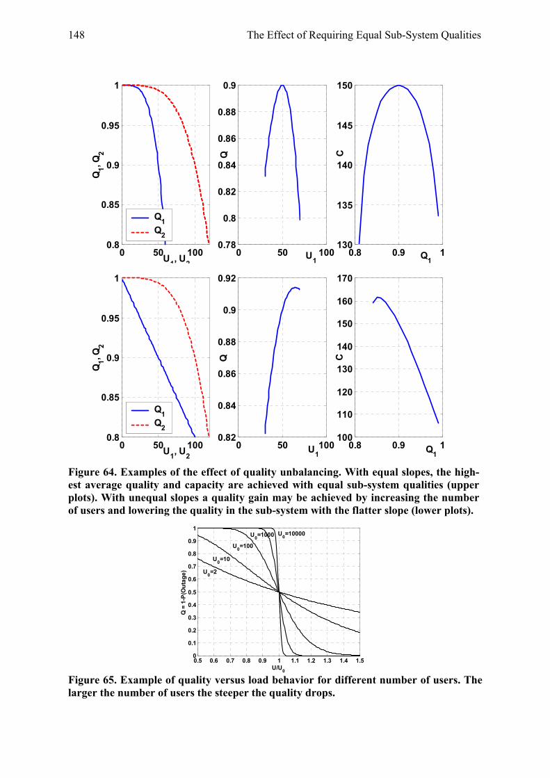
148 The Effect of Requiring Equal Sub-System Qualities
0 50 1000.8
0.85
0.9
0.95
1
U1, U2
Q1, Q
2
Q1Q2
0 50 1000.78
0.8
0.82
0.84
0.86
0.88
0.9
U1
Q
0.8 0.9 1130
135
140
145
150
Q1
C
0 50 1000.8
0.85
0.9
0.95
1
U1, U2
Q1, Q
2
Q1Q2
0 50 1000.82
0.84
0.86
0.88
0.9
0.92
U1
Q
0.8 0.9 1100
110
120
130
140
150
160
170
Q1
C
Figure 64. Examples of the effect of quality unbalancing. With equal slopes, the high-est average quality and capacity are achieved with equal sub-system qualities (upper plots). With unequal slopes a quality gain may be achieved by increasing the number of users and lowering the quality in the sub-system with the flatter slope (lower plots).
0.5 0.6 0.7 0.8 0.9 1 1.1 1.2 1.3 1.4 1.50
0.1
0.2
0.3
0.4
0.5
0.6
0.7
0.8
0.9
1
U/U0
Q =
1-P
(Out
age) U0=2
U0=10
U0=100
U0=1000 U0=10000
Figure 65. Example of quality versus load behavior for different number of users. The larger the number of users the steeper the quality drops.

149
Appendix D Per-Service Capacity and Interference Balancing Proofs
In this appendix, two similar proofs are given for that per-service capacity balancing and in-terference balancing maximizes overall capacity.
Proposition: For cases where assumptions (i) - (iii) in Section 4.1.1 are valid, a necessary and sufficient requirement for maximized capacity is that all per-service capacities are equal:
knCrCrC kknn ,)())(,())(,( ∀== ααααα rrrrr (170)
Proof: In an unbalanced case, assume that:
)())(,())(,( ααααα rrrrr CrCrC kknn => (171)
where Ck(αr ,rk(αr )) is the smallest per-service capacity. Then a resource reallocation ∆r ex-ists so that:
)()())(,())(,( αααααα rrrrrr CCrrCrrC kknn >′=∆+=∆− (172)
Hence, in an unbalanced case a higher overall capacity can always be found by reallocating resources. Equation (43) is thus a necessary requirement for maximized capacity.
Further, since 0)(/)( <∂∂ αα rrkn rr for n ≠ k, any resource allocation that deviates from Equa-
tion (170) must relative to this reference case reduce the amount of resources allocated to at least one bearer service. Assume e.g. that compared to the balanced case in Equation (170) the resource amount allocated to bearer service l is reduced by ∆rl, then:
)())(,()())(,( αααααα rrrrrr CrCCrrC lllll =<′′=∆− (173)
Bearer service l hence limits the overall capacity to a lower value than in the balanced case. Since this is valid for any resource allocation that deviates from Equation (170), it is a suffi-cient requirement for a maximum of overall capacity.
Proposition: A necessary and sufficient requirement for maximized capacity in interference limited systems, as defined in Section 4.2.1, is that the maximum interference levels are equal for all bearer services:
knPiPi kknn ,))(,())(,( maxmax ∀= αααα rrrr (174)
Proof: In an unbalanced case, assume that:
)())(,())(,( maxmaxmax ααααα rrrrr iPiPi kknn => (175)
where imax k(αr ,Pk(αr )) is the smallest maximum interference level. Then a power realloca-tion ∆P exists so that:
)()())(,())(,( maxmaxmaxmax αααααα rrrrrr iiPPiPPi kknn >′=∆+=∆− (176)
Hence, in an unbalanced case a higher overall maximum interference, and hence an in-creased overall capacity since C(αr ) is strictly growing with increasing imax(αr ), can always be found by reallocating power budgets. Equation (174) is thus a necessary requirement for maximized capacity.

150 Per-Service Capacity and Interference Balancing
Further, since 0)(/)( <∂∂ αα rrkn PP for n ≠ k, any resource allocation that deviates from Equa-
tion (174) must relative to this reference case reduce the power allocated to at least one bearer service. Assume e.g. that compared to the balanced case in Equation (174)the power allocated to bearer service l is reduced by ∆Pl, then:
)())(,()())(,( maxmaxmaxmax αααααα rrrrrr iPiiPPi lllll =<′′=∆− (177)
Bearer service l hence limits the maximum interference level to a lower value than in the balanced case. Since the overall capacity C(αr ) is strictly growing with increasing imax(αr ), also this is limited to a lower value than in the balanced case. Since this is valid for any re-source allocation that deviates from Equation (174), it is a sufficient requirement for a maximum of overall capacity.

151
Appendix E Additional GSM/EDGE Results
In this appendix some additional capacity regions for GSM/EDGE are presented. These are taken from [86], and derived under slightly different assumptions than those presented in Chapter 5, which explains the slightly different absolute capacity results.
Figure 66 (left) shows simulated capacity regions with EFR voice bearers and single-slot data bearers with CSE bitrate requirement of 10kbps. In addition to the reference case with equal powers, and the interference balancing solution, here achieved with a power offset of 6dB (the difference from the 5dB offset of Section 5.4.1 is due to more robust data bearers), results achieved with power offsets of 3dB and 9dB are also included. It is seen that among the alternative offsets, the interference balancing solution of 6dB does indeed provide the highest capacity. The capacity achieved with isolated resources is also included. In this case, the available timeslots are divided into fixed voice and data groups (different divisions have to be made for different service mixes). As expected from the discussion in Section 4.1.3, it is seen that this solution results in a concave capacity region. The reason is that when divid-ing the timeslots into separate pools, these pools become smaller that the full pool size, and the trunking efficiency reduces, i.e. each timeslot becomes less efficient, see further [86].
In the right plot in Figure 66 a CSE bitrate requirement of 20kbps is used. It is now seen that, as expected from Figure 20, a power offset of 3dB yields better performance than using 0dB or 6dB.
0 5 10 15 200
0.1
0.2
0.3
0.4
0.5
0.6
0.7
0.8
Voice Capacity [Erlang/MHz/site]
Inte
ract
ive
Dat
a C
apac
ity [b
ps/H
z/si
te] Pdata = Pvoice
Pdata = Pvoice - 3 dBPdata = Pvoice - 6 dBPdata = Pvoice - 9 dBIsolated Resources
0dB
3dB 9dB 6dB
iso
0 5 10 15 200
0.1
0.2
0.3
0.4
0.5
0.6
Voice Capacity [Erlang/MHz/site]
Inte
ract
ive
Dat
a C
apac
ity [b
ps/H
z/si
te] Pdata = Pvoice Pdata = Pvoice - 3 dBPdata = Pvoice - 6 dB
3dB
0dB
6dB
Figure 66. Additional capacity regions for GSM/EDGE. Left: Capacity regions with EFR voice bearers and single-slot data bearers with 10kbps CSE requirement for a set of power offsets and with isolated resources. Right: Capacity regions with a CSE bi-trate requirement of 20kbps.

153
Appendix F Additional WCDMA/HSDPA Results
This appendix presents capacity regions for some additional scenarios not covered in Chapter 7. Figure 67 shows simulated and theoretical capacity regions achieved with a Pe-destrian A channel and a maximum voice bearer power of 6W, but with CSE bitrate re-quirements of 150kbps and 300kbps for WWW users. It is seen that for these higher CSE requirements the data capacity is somewhat reduced. The small reduction depends on that close to the capacity limit the CSE bitrate falls rapidly with the traffic load. The convex shape of the capacity regions remains.
Figure 68 shows simulated and theoretical capacity regions achieved with voice bearers us-ing DTX for both Pedestrian and Typical Urban channels. As might be expected, it is seen that significantly higher voice capacities are achieved with DTX. The convex shape of the capacity regions however remains.
0 1 2 3 4 5 6 70
50
100
150
200
250
300
350
Voice Capacity [Erlang/MHz/Sector]
WW
W C
apac
ity [k
bps/
MH
z/Se
ctor
]
SimulationTheory
0 1 2 3 4 5 6 70
50
100
150
200
250
300
Voice Capacity [Erlang/MHz/Sector]
WW
W C
apac
ity [k
bps/
MH
z/Se
ctor
]
SimulationTheory
Figure 67. Simulated and theoretical capacity regions for CSE bitrate requirements of 150kbps (left) and 300kbps (right). Pedestrian A channel, Pmax v = 6W.
0 2 4 6 8 100
50
100
150
200
250
300
350
Voice Capacity [Erlang/MHz/Sector]
WW
W C
apac
ity [k
bps/
MH
z/Se
ctor
]
SimulationTheory
0 2 4 6 8 10 12 140
50
100
150
200
250
Voice Capacity [Erlang/MHz/Sector]
WW
W C
apac
ity [k
bps/
MH
z/Se
ctor
]
SimulationTheory
Figure 68. Simulated and theoretical capacity regions for voice bearers with DTX. Left: Pedestrian A channel, Pmax v = 6W; Right: Typical Urban Channel, Pmax v = 1W.


155
Appendix G A Graphical Method for Finding Near-Optimum Bearer Service Allocations
The results derived in Section 8.2 may also be obtained by the simple graphical method de-picted in Figure 69. This method was proposed by Magnus Almgren, and is not an original contribution of this author. The method is included here to show that solutions similar to those of Section 8.2 may be expected also when the sub-system capacity region limits are not continuously differentiable. The method also helps in getting an intuitive feeling for what bearer service allocation solutions and combined capacity regions may be expected.
Using the graphical method, the capacity region of one of the sub-systems is first mirrored, and its origin is put on a line corresponding to the fixed service mix in question. By then moving the mirrored capacity region as far outwards as possible, while it still has a coincid-ing point with the other capacity region, the near-optimum bearer service allocations are found. The intersection of the two capacity regions at this point is located at the near-optimum bearer service allocations (v1
*, d1*) and (v2
*, d2*). The origin of the mirrored capac-
ity region is further located at (v, d), i.e. at the near-optimum combined capacity.
Obviously, if the intersection of the capacity regions occurs at inner points of the capacity regions, i.e. between the single bearer service endpoints, the two derivatives are as seen in Figure 69 equal. It is further easily seen that if both capacity regions are convex, there will be an inner maximum, and hence bearer services should be mixed within the sub-systems. If both capacity regions are concave on the other hand, the intersection will always occur at an extreme point of the capacity regions, indicating that bearer services should be separated into different sub-systems.
(v2,d2)
(v1,d1)
(v,d)
voice
data
Figure 69. Two-bearer service capacity regions for two different sub-systems and graphical derivation of the near-optimum bearer service allocations and combined ca-pacity region.


157
Appendix H Performance with Equal Service Mixes in Sub-Systems
This appendix derives the combined capacity region for a two-service, two-access case with linear sub-system capacity regions, for which an equal service mix bearer service allocation strategy is used.
A straight line between the points (V, 0) and (0, D) may be represented in polar form by the radius r and angle ϕ as:
)cos()sin(
)(ϕϕ
ϕDVDVr
+⋅
= (178)
In our case V and D correspond to single-bearer service endpoints, and ϕ is a simple function of the service mix αr . A two-access system with linear sub-system capacity regions, and equal service mixes in the two sub-systems, will thus have a combined capacity region de-limited by:
)cos()sin()cos()sin(
)()()(22
22
11
1121 ϕϕϕϕ
ϕϕϕDVDV
DVDVrrrtot +
⋅+
+⋅
=+= (179)
From testing this appears to be a concave function unless V1 = V2 and D1 = D2. Two exam-ples are given in Figure 70. When the single-bearer service endpoints differ only a little, as in the left plot, the combined capacity region is close to linear. With larger differences in the single-bearer service endpoints however, as in the right plot, the combined capacity region gets dramatically poorer.
0 5 10 15 20 25 300
5
10
15
20
25
30
Voice Users
Dat
a U
sers
Sub-system 1Sub-system 2Combined
0 10 20 30 40 50 600
10
20
30
40
50
60
Voice Users
Dat
a U
sers
Sub-system 1Sub-system 2Combined
Figure 70. Two cases of combined capacity regions with equal service mix in the sub-systems.

TRITA-S3-RST-0302ISSN 1400-9137
ISRN KTH/RST/R--03/02--SE
Radio Communications Systems Lab. Dept. of Signals, Sensors and Systems Royal Institute of Technology SE-100 44 Stockholm, Sweden