radiological engineering lab manualhomepages.rpi.edu/~xug2/courses/labman.pdf · radiological...
TRANSCRIPT
RADIOLOGICAL ENGINEERING LAB MANUAL
Instructors:
George Xu ([email protected]) Peter Caracappa ([email protected])
Mark Furler ([email protected])
SPRING 2006
Radiological Engineering Lab Manual 2006 ________________________________________________________________________
TABLE OF CONTENTS
LAB REPORT GUIDELINES…………………………………………................ 3 LAB #1. PROPORTIONAL COUNTER AND AUTOMATIC SAMPLER CHANGER SYSTEM.............5 LAB #2. CALIBRATION OF GAMMA SOURCE AND RADIATION SURVEY METERS ................10 LAB #3. GAMMA SPECTROMETRY USING NAI(TL) AND HPGE DETECTORS …………….... 15 LAB #4. APPLICATION OF COMPUTER CODES FOR RISK ASSESSMENT INVOLVING RELEASE OF RADIOACTIVE MATERIALS INTO THE ENVIRONMENT .....................................................22 LAB #5. RADIATION DETECTION WITH THERMO-LUMINESCENT DOSIMETERS (TLD) AND THE MOSFET DOSIMETER SYSTEM....................................................................................30 LAB #6. AIR SAMPLING FOR RADON…………………………………………………… ..33 LAB #7. RADIATION SURVEY AND CONTAMINATION CONTROL AT RPI FACILITIES ..........35 LAB #8. CALCULATION OF SHIELD THICKNESS USING MONTE CARLO CODE….................39
2
Radiological Engineering Lab Manual 2006 ________________________________________________________________________
LAB REPORT GUIDELINES The labs for this course are meant to be instructive as to methods and procedures beneficial to the study of health physics. The procedures outlined in each experiment are as complete as possible. At times, however, it may be necessary to consult additional materials, either in the operation of the lab or the data analysis and discussion of the results. Manuals for the operation of the lab equipment will be available in the lab. Ask the lab instructor if you need assistance.
Lab reports are due a week from the date that the lab is performed (the specific due date will be announced in the lab for the Navy Nuclear students). Late submissions are subject to penalty. Your lab report is not only a record of the work you have completed, but an explanation of that work to others. The report should be addressed to someone that has a basic knowledge of the principles of health physics, but may not be familiar with the particular equipment or procedures used in your lab. The report should contain the following basic elements: COVER Student Name, Team Members, Experiment Title, Date, etc. ABSTRACT A short paragraph summarizing the results obtained during the lab. A good abstract explains to the reader the purpose and importance of the lab, briefly summarizes what was done in the lab, and provides the numerical results from it. In essence, the abstract is meant to convince the reader that it is worth it to him or her read the rest of the lab. OBJECTIVE This is a well-formulated sentence (or two at the most) that explains why it is important to do this lab, and how it applies to the field of health physics. THEORY This section contains a description of the theoretical basis for the lab. It also describes the experimental setup and the experimental procedure in general terms (it is not necessary to list every detailed step of the procedure, but it should describe what actions were taken). Cite references if necessary. DATA Present data appropriately (typically in tabular and graphical forms). Please give a title and a number to figures and graphs. Be sure to include sample calculations for any data analysis or error analysis that you perform. Calculations that are incorrect without any explanation of how they came about cannot be credited.
3
Radiological Engineering Lab Manual 2006 ________________________________________________________________________
DISCUSSION This is the most important section of the lab report. You should discuss what your data means and your confidence in the data (how good is it and why?). Also, discuss any assumptions that you made in the lab or report. You should also answer any questions that may be presented in the lab manual (not in a question-response form – the questions should be addressed in a narrative way in the text). You also need to address why it is you did this lab, meaning how your objective was fulfilled. Many years from now, you may find a detailed report of yours extremely useful. GOING FURTHER What additional experimentation might you do that would contribute to using the lab as a tool of health physics? Or alternatively, how could this lab procedure be improved to better illustrate the principles it is trying to address? Obviously, reports should be typed and easy to read, and should be as professional as possible. You should write your own report and share only the data. Use as many pages as needed, but a report usually is 4-6 pages long (not including charts, figures, or attachments). Make sure you answer all the questions in the lab. Each lab will be graded out of a total of 10 points. In general, the points are broken down by: abstract (1 point), objective (1 point), theory (1 point), data (2 points), discussion (3 points), going further (1 point), and the overall appearance and quality of the work (1 point). However, this is not a strict system, and an exceptional job on one section may help boost the grade on a section that was a little weaker (but don’t count on it – aim for a balanced report!)
ANY ADDITIONAL QUESTIONS ABOUT THE LABS OR THE LAB REPORTS MAY BE ADDRESSED TO THE LAB INSTRUCTOR.
4
Radiological Engineering Lab Manual 2006 ________________________________________________________________________
LAB #1 PROPORTIONAL COUNTER AND AUTOMATIC SAMPLE
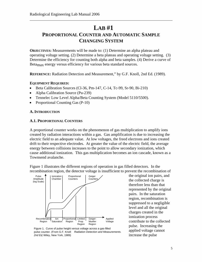
CHANGING SYSTEM OBJECTIVES: Measurements will be made to: (1) Determine an alpha plateau and operating voltage setting. (2) Determine a beta plateau and operating voltage setting. (3) Determine the efficiency for counting both alpha and beta samples. (4) Derive a curve of Betamax energy versus efficiency for various beta standard sources. REFERENCE: Radiation Detection and Measurement,” by G.F. Knoll, 2nd Ed. (1989). EQUIPMENT REQUIRED: • Beta Calibration Sources (Cl-36, Pm-147, C-14, Tc-99, Sr-90, Bi-210) • Alpha Calibration Source (Pu-239) • Tennelec Low Level Alpha/Beta Counting System (Model 5110/5500). • Proportional Counting Gas (P-10) A. INTRODUCTION A.1. PROPORTIONAL COUNTERS A proportional counter works on the phenomenon of gas multiplication to amplify ions created by radiation interactions within a gas. Gas amplification is due to increasing the electric field to an adequate value. At low voltages, the freed electrons and ions created drift to their respective electrodes. At greater the value of the electric field, the average energy between collisions increases to the point to allow secondary ionization, which cause additional ionization. This gas multiplication becomes an ion cascade, known as a Townsend avalanche. Figure 1 illustrates the different regions of operation in gas filled detectors. In the recombination region, the detector voltage is insufficient to prevent the recombination of
the original ion pairs, and the collected charge is therefore less than that represented by the original pairs. In the saturation region, recombination is suppressed to a negligible level and all the original charges created in the ionization process contribute to the collected pulse. Increasing the applied voltage cannot increase the pulse
IonizationChamber
ProportionalCounters
GeigerCounters
IonSaturation
ProportionalRegion
LimitedProp.
Region
Geiger-MuellerRegion
RecombinationRegion
PulseAmplitude(log Scale)
AppliedVoltage
Figure 1. Curve of pulse height versus voltage across a gas-filledpulse counter. (From G.F. Knoll: Radiation Detection and Measurements.2nd Ed., Wiley, New York, 1989)
5

Radiological Engineering Lab Manual 2006 ________________________________________________________________________
amplitude because all charges are already collected and their formation rate is constant (ion saturation). As the detector voltage increases into the proportional region, the threshold field necessary to cause gas amplification is reached. In a portion of the region, the gas multiplication is linear and the collected charge is proportional to the original number of ion pairs formed by the radiation interaction. As detector voltage increases, into the limited proportional region, some nonlinearities will be observed, caused by the pulse amplitude no longer being proportional to the original pairs. When the detector voltage enters the Geiger-Mueller region, the avalanche proceeds until a sufficient number of positive ions are created to reduce the electric field below the point that additional gas amplification can occur. In this experiment, the Tennelec LB5100/5500 Alpha/Beta gas flow proportional counter is used; it operates in the proportional region. A.2. ALPHA AND BETA PLATEAUS
Proportional counters can be used to distinguish between alpha and beta sources. For charged particles, such as alphas and betas, a signal is generated for each particle that deposits a sufficient amount of energy to the fill gas of the detector. Low values of gas amplification are typically used which requires that the
detection of the original pulse originate from the number of ion pairs in order to exceed the discrimination level of the system. For alpha counting, the differential pulse height spectrum (DPHS) has a single isolated peak as shown in Figure 2, since nearly all pulses from the detector are due to monoenergetic alpha particles. This peak results in a simple plateau if the detector dimensions are large compared to the range of the particle, which is usually the case with alphas. For beta particles, the particle range usually greatly exceeds the chamber dimensions. The ion pairs formed in the gas are then proportional to only that small fraction of the particle energy lost in the gas before reaching the opposite wall of the chamber. Additionally, due to the non-monoenergetic nature of beta particles, the generated beta pulse will be broader than a pulse generated by alpha and will be smaller in height. This leads to the formation of a second plateau, the beta plateau, in which both alpha and beta interactions are counted. This can be seen in Figure 3.
dNdH
H
CountRate
V
Counting CurveDPHS
Figure 2. Typical DPHS and Counting Curve for alpha particles. (From G.F. Knoll: Radiation Detection and Measurements. 2d Ed., Wiley, New York, 1989)
Because the beta particle pulse height distribution is broader and less well separated from the low-amplitude noise, the beta plateau is generally shorter and shows a greater slope than the alpha plateau.
dNdH
H
CountRate
V
Counting Curve
DPHS
Figure 3. Typical DPHS and Counting Curve for alpha and beta particles. (From G.F. Knoll: Radiation Detection and Measurements. 2d Ed., Wiley, New York, 1989)
Beta plateau
alpha plateau
alpha
beta
The plateaus are used to identify operating voltages,
6
Radiological Engineering Lab Manual 2006 ________________________________________________________________________
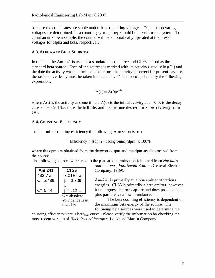
because the count rates are stable under these operating voltages. Once the operating voltages are determined for a counting system, they should be preset for the system. To count an unknown sample, the counter will be automatically operated at the preset voltages for alpha and beta, respectively. A.3. ALPHA AND BETA SOURCES In this lab, the Am-241 is used as a standard alpha source and Cl-36 is used as the standard beta source. Each of the sources is marked with its activity (usually in µCi) and the date the activity was determined. To ensure the activity is correct for present day use, the radioactive decay must be taken into account. This is accomplished by the following expression:
A t A e t( ) ( )= −0 λ where A(t) is the activity at some time t, A(0) is the initial activity at t = 0, λ is the decay constant = .6931/t1/2, t1/2 is the half life, and t is the time desired for known activity from t = 0. A.4. COUNTING EFFICIENCY To determine counting efficiency the following expression is used: Efficiency = [(cpm - background)/dpm] x 100% where the cpm are obtained from the detector output and the dpm are determined from the source. The following sources were used in the plateau determination (obtained from Nuclides
and Isotopes, Fourteenth Edition, General Electric Company, 1989): Am-241 is primarily an alpha emitter of various energies. Cl-36 is primarily a beta emitter, however it undergoes electron capture and does produce beta plus particles at a low abundance.
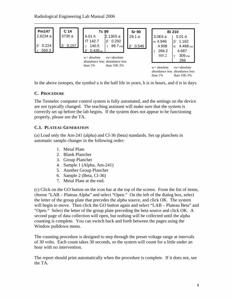
The beta counting efficiency is dependent on the maximum beta energy of the source. The following beta sources were used to determine the
counting efficiency versus betamax curve. Please verify the information by checking the most recent version of Nuclides and Isotopes, Lockheed Martin Company.
Cl 36 3.01E5 a β - 0.709 ε β + .12 w
w= absolute abundance less than 1%
Am 241 432.7 a α - 5.486 α + 5.44
7
Radiological Engineering Lab Manual 2006 ________________________________________________________________________
Pm1472.6234 a
β- 0.224γ 550.3
C 145730 a
β- 0.157
Sr 9029.1 a
β- 0.546
Tc 996.01 h 2.13E5 aIT 142.7 β- 0.292γ 140.5 γ 89.7 vwβ- 0.435 w
vw=absoluteabundance lessthan 10E-3%
w= absoluteabundance lessthan 1%
Bi 2103.0E6 a 5.01 dα 4.946 β- 1.162 4.908 α 4.468 vwγ 266.2 4.687 305.2 γ 305 vw 266
vw=absoluteabundance lessthan 10E-3%
w= absoluteabundance lessthan 1%
In the above isotopes, the symbol a is the half life in years, h is in hours, and d is in days. C. PROCEDURE
The Tennelec computer control system is fully automated, and the settings on the device are not typically changed. The teaching assistant will make sure that the system is correctly set up before the lab begins. If the system does not appear to be functioning properly, please see the TA. C.1. PLATEAU GENERATION
(a) Load only the Am-241 (alpha) and Cl-36 (beta) standards. Set up planchets in automatic sample changer in the following order:
1. Metal Plate 2. Blank Planchet 3. Group Planchet 4. Sample 1 (Alpha, Am-241) 5. Another Group Planchet 6. Sample 2 (Beta, Cl-36) 7. Metal Plate at the end.
(c) Click on the GO button on the icon bar at the top of the screen. From the list of items, choose “LAB – Plateau Alpha” and select “Open.” On the left of the dialog box, select the letter of the group plate that precedes the alpha source, and click OK. The system will begin to move. Then click the GO button again and select “LAB – Plateau Beta” and “Open.” Select the letter of the group plate preceding the beta source and click OK. A second page of data collection will open, but nothing will be collected until the alpha counting is complete. You can switch back and forth between the pages using the Window pulldown menu. The counting procedure is designed to step through the preset voltage range at intervals of 30 volts. Each count takes 30 seconds, so the system will count for a little under an hour with no intervention. The report should print automatically when the procedure is complete. If it does not, see the TA.
8

Radiological Engineering Lab Manual 2006 ________________________________________________________________________
(c) Analyze the plot and verify that you agree with the operating voltage that the computer has chosen. C.2. COUNTING EFFICIENCY
(a) Load planchets in the system with a metal plate first, a blank planchet, a group planchet, a planchet with the Pu-239 source, and planchets with the beta sources that you have available to you (be sure you know which order they are in). (b) Run the “LAB – Efficiency” procedure. (c) The system will count each source for two minutes, and print out the average counts per minute (cpm). Background is already corrected for in this value. (d) The disintegration per minute (dpm) for the standards are known. Calculate counting efficiency of the system for alphas and betas by: Efficiency = [cpm/dpm] X 100%. (e) Use the standard deviation reported by the computer to calculate the standard deviation in the efficiencies for each source. (f) For the efficiencies calculated for each beta source, plot a curve of efficiency vs. Betamax energy. Information on Betamax energy can be found on the Chart of Nuclides in the lab manual. (Please remember that Sr-90 decays to yield Y-90 which emits beta particles at a maximum energy of 2.28 MeV.) C. 3. CROSSTALK MEASUREMENT In order to differentiate between alpha and beta counts, a specific energy level is chosen to discriminate between the two. If counts from one type of source are counted in the other region, this is called crosstalk. Estimate the crosstalk in the system by setting it up to count a single planchet that is holding both the Clorine-36 and the Americium-241 sources (be careful not to damage the Am-241 source, or to lay the sources on top of each other). Run the efficiency procedure, and compare the alpha and beta counts in this measurement to the counts generated for those sources in the last section of the lab. D. QUESTIONS Consider these additional questions in your discussion: (a) Why is advantageous to operate in the plateau region? (b) The system corrects for background using measurements previously taken over very
long counting times. What is the source of that background, and why is it so much higher for beta than it is for alpha?
(c) Describe a possible use for this device in radiation protection or health physics, and explain how these experimental procedures would be used in it.
9

Radiological Engineering Lab Manual 2006 ________________________________________________________________________
LAB #2 CALIBRATION OF GAMMA SOURCE AND RADIATION SURVEY
METERS OBJECTIVES: To learn how to calibrate a gamma standard source with NIST traceable Condenser R. Chambers and use that information to calibrate radiation survey meters. REFERENCE: “Radiation Detection and Measurement,” by G.F. Knoll, 2nd Ed. (1989). EQUIPMENT REQUIRED: • Cs-137 Source • Meter Stick • Victoreen Condenser “R” Chamber • Timer • Portable Ion Chambers and GM counters for gamma radiation A. INTRODUCTION This laboratory experiment uses a 5 Ci Cs-137 as the source for gamma radiation exposure. The decay scheme for Cs-137 is as follows:
The beta decay is a relatively slow process characterized by a half-life of hundreds of days or greater (30.17 years for Cs-137), whereas the excited state in the daughter nucleus (Ba) has a much shorter average lifetime (on the order of picoseconds or less). Deexcitation takes place through the emission of a gamma-ray whose energy is 0.662 MeV. This is the radiation source that the Victoreen Condenser “R” chambers and the PICs are exposed to. The beta radiation won’t penetrate the detector.
β− , 93.5%
0
Cs137
55
Ba137
56
γ = 0.662 MeV
β −
6.5%
Figure 1: The decay scheme for Cs-137
0.662 MeV
The Cs-137 source is small in size and may be treated as a point source for dose calculations. The exposure rate decreases by a factor of 1/x2, as the distance x increases. The source is always kept inside a heavy lead shielding so the exposure rate around the shielding is not very high. A window, when opened, allows collimated gamma rays to pass through the shielding without attenuation. Small lead attenuators, each of ½” thick, may be added to reduce the gamma exposure rate to desired levels at different distances.
10
Radiological Engineering Lab Manual 2006 ________________________________________________________________________
The measurement devices in this experiment are the Victoreen Condenser “R” Chambers. To measure radiation dose, the response of the instrument must be proportional to the absorbed energy. These devices are basically “air wall” ionization chambers.
The condenser type of detectors is of the indirect reading type; an auxiliary device is necessary in order to read the measured dose. This device measures radiation dose in roentgens, and most condenser-type dosimeters measure integrated X-ray or gamma ray exposures up to 200 mR with an accuracy of ± 15% for quantum energies between about 0.05 and 2 MeV. The calibration of the Cs-137 source is accomplished by using Condenser Chambers that are pre-calibrated at National Institute of Standards and Technology (NIST). All calibrations have to be traceable to NIST. Exposure of the R Chamber at a specific distance from the Cs-137 source for a known period of time provides a calibration point. The exposure rate in Roentgen per hour (R/hour) is determined as follows: R/hour = (X)(CFINST)(CFTP)/(Exposure Time (Hours)) where,
X = Condenser R Chamber reading CFINST = Chamber calibration factor CFTP = Instrument Temperature-Pressure calibration factor.
The R Chamber is discharged and zeroed after each time it is read. The R Chamber is placed on the charger-reader. A hairline intersects the axis of the exposure in R. If the 0.025r chamber is used, the reading should be divided by 1000 (on the 20 scale) to determine the exposure. If the 0.25r chamber is used, the reading should be divided by 100 (on the 20 scale) to determine the exposure. Once the exposure is read, the R chamber is zeroed by pushing the wheel on the left up quickly and then back and hold it in the back position. While holding use the dial to the right to adjust the hairline back to zero.
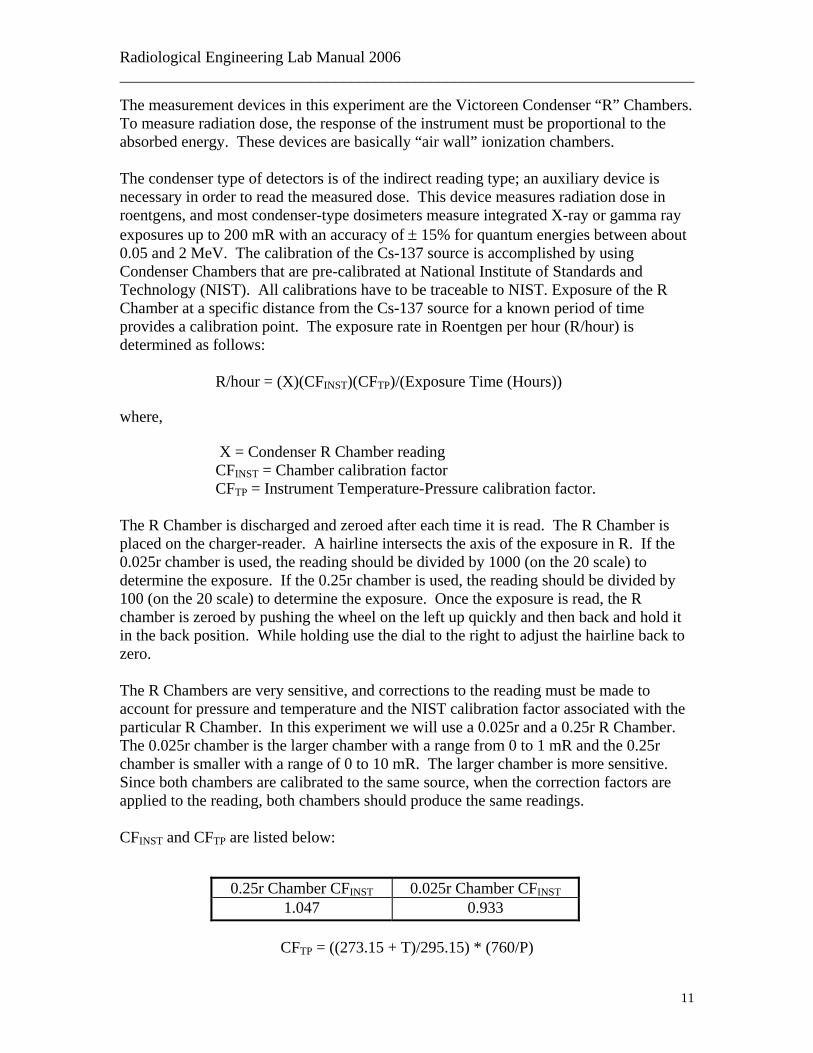
The R Chambers are very sensitive, and corrections to the reading must be made to account for pressure and temperature and the NIST calibration factor associated with the particular R Chamber. In this experiment we will use a 0.025r and a 0.25r R Chamber. The 0.025r chamber is the larger chamber with a range from 0 to 1 mR and the 0.25r chamber is smaller with a range of 0 to 10 mR. The larger chamber is more sensitive. Since both chambers are calibrated to the same source, when the correction factors are applied to the reading, both chambers should produce the same readings. CFINST and CFTP are listed below:
0.25r Chamber CFINST 0.025r Chamber CFINST1.047 0.933
CFTP = ((273.15 + T)/295.15) * (760/P)
11
Radiological Engineering Lab Manual 2006 ________________________________________________________________________
The procedures for this experiment are rather simple. Measurements should be made at various distances using both the unshielded and shielded source. The measurements are taken with both R chambers. Make measurements at 3 distances for each R Chamber with and without the shield present. Distances and times for the required exposure can be determined from the calibration curve on display in the source room. The corrected readings (instrument calibration, temperature, pressure adjustment calibration) will produce a dose rate that can be used to plot dose rate (mR/hour) versus the distance (cm) from the source. This will produce a calibration curve. When a NIST traceable calibration is performed on the gamma source, that source can then be used to verify the calibrations of other radiation survey meters. The meter calibrations are necessary and should be repeated every year, following repair, or when deemed necessary, i.e. thought to be out of calibration. Calibration should be considered acceptable when the instrument responds to better than ±10% of the radiation level being measured either by a direct meter response or a pre-determined calibration curve.
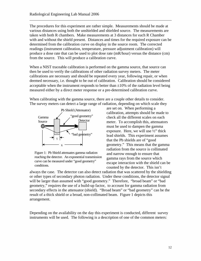
When calibrating with the gamma source, there are a couple other details to consider. The survey meters can detect a large range of radiation, depending on which scale they
are set on. When performing a calibration, attempts should be made to check all the different scales on each meter. To accomplish this, attenuators must be used to dampen the gamma exposure. Here, we will use ½” thick lead shields. This experiment assumes that the Pb shields are of “good geometry.” This means that the gamma radiation from the source is collimated and narrow enough to ensure that gamma rays from the source which escape interaction with the shield can be counted by the detector. This isn’t
always the case. The detector can also detect radiation that was scattered by the shielding or other types of secondary photon radiation. Under these conditions, the detector signal will be larger than assumed with “good geometry.” Therefore, “broad beam” or “bad geometry,” requires the use of a build-up factor, to account for gamma radiation from secondary effects in the attenuator (shield). “Broad beam” or “bad geometry” can be the result of a thick shield or a broad, non-collimated beam. Figure 1 depicts this arrangement.
GammaSource
Pb Shield (Attenuator)
Detector
x
t
Figure 1: Pb Shield attenuates gamma radiationreaching the detector. An exponential transmissioncurve can be measured under “good geometry”conditions.
“good geometry”
“bad geometry”
Depending on the availability on the day this experiment is conducted, different survey instruments will be used. The following is a description of one of the common meters:
12
Radiological Engineering Lab Manual 2006 ________________________________________________________________________
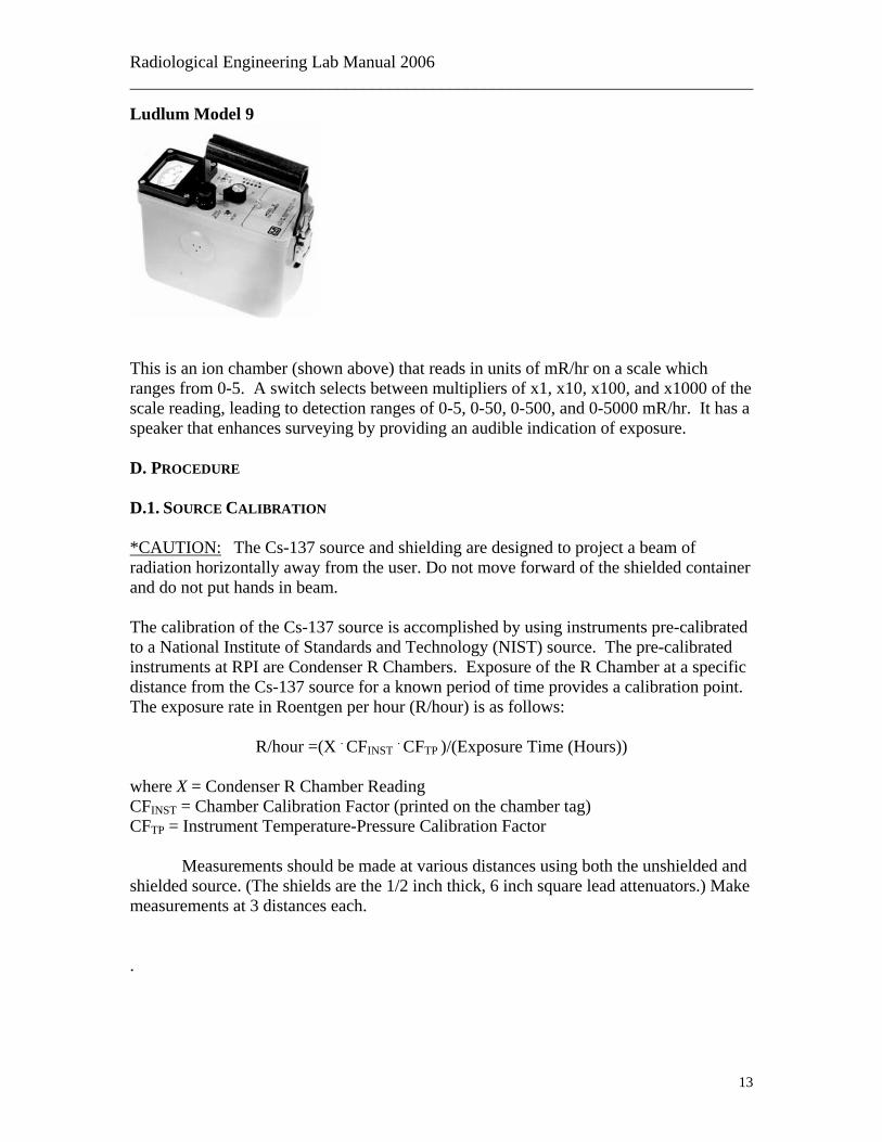
Ludlum Model 9
This is an ion chamber (shown above) that reads in units of mR/hr on a scale which ranges from 0-5. A switch selects between multipliers of x1, x10, x100, and x1000 of the scale reading, leading to detection ranges of 0-5, 0-50, 0-500, and 0-5000 mR/hr. It has a speaker that enhances surveying by providing an audible indication of exposure. D. PROCEDURE D.1. SOURCE CALIBRATION *CAUTION: The Cs-137 source and shielding are designed to project a beam of radiation horizontally away from the user. Do not move forward of the shielded container and do not put hands in beam. The calibration of the Cs-137 source is accomplished by using instruments pre-calibrated to a National Institute of Standards and Technology (NIST) source. The pre-calibrated instruments at RPI are Condenser R Chambers. Exposure of the R Chamber at a specific distance from the Cs-137 source for a known period of time provides a calibration point. The exposure rate in Roentgen per hour (R/hour) is as follows:
R/hour =(X . CFINST . CFTP )/(Exposure Time (Hours)) where X = Condenser R Chamber Reading CFINST = Chamber Calibration Factor (printed on the chamber tag) CFTP = Instrument Temperature-Pressure Calibration Factor Measurements should be made at various distances using both the unshielded and shielded source. (The shields are the 1/2 inch thick, 6 inch square lead attenuators.) Make measurements at 3 distances each. .
13
Radiological Engineering Lab Manual 2006 ________________________________________________________________________
D.2. RADIATION SURVEY METER CALIBRATION 1. Using the information for exposure dose rate vs. distance, determine a combination
of various attenuators and distance to provide three exposure dose rates for each range of the survey meter. (The 20%, 50% and 80% Full Scale Readings). Follow the manufacturer's instructions for operation of the survey meters. Check the survey meter to assure it is working properly (battery check, zero, etc.).
2. Place the survey meter at the pre-determined distance with the necessary attenuators
in place. 3. Turn the survey meter on to the proper range. 4. Assure everyone is behind the shield. 5. Turn the source on by pulling the source handle to refusal (alarm light be activated). 6. Record instrument reading. 7. Repeat for various survey meter ranges at predetermined distances and other
attenuators. 8. Return source to stored position when not in use. Results 1. Explain briefly how the survey meter will be used in health physics operation. 2. Plot the exposed dose rate vs. the meter response. 3. Does the survey meter you calibrated meet the criteria of 10% at each of the 3 points on each scale?
14

Radiological Engineering Lab Manual 2006 ________________________________________________________________________
LAB #3 GAMMA-RAY SPECTROSCOPY USING NaI(Tl)
AND HPGE DETECTORS OBJECTIVES: (1) To gain familiarity with the NaI(Tl) and HPGe systems through use of
standard sources. (2) To compare gamma spectroscopy with the NaI (Tl) and HPGe detectors . (3)To determine the composition of an unknown from its gamma energy spectrum (isotope identification).
REFERENCES: “Radiation Detection and Measurement” by G. F. Knoll, 2nd Ed. (1989) “The Gamma Rays of the Radionuclides” by G. Erdtmann and W. Soyka (1979) “Scintillation Spectrometry - Gamma Ray Spectrum Catalog” by R. L. Heath EQUIPMENT REQUIRED:
• NaI(Tl) Scintillation Detector, Photomultiplier Tube and Base, and Pb Shield • HPGe Portable Detector • IBM-PC Computer and Genie-2000 Analyzer • InSpector2000 Multi Channel Analyzer and High Voltage Supply • Standard Gamma Sources and Unknown Source
A. INTRODUCTION A.1 GAMMA-RAYS The gamma-ray energies emitted by various radionuclides are unique for each species; and they are said to “fingerprint” the material. Determination of the quality and quantity of a gamma spectrum can identify minute quantities of an element within an “unknown sample.” In this laboratory, you will acquaint yourself with the Thallium-activated Sodium Iodide (NaI(Tl)) and High Purity Germanium (HPGe) systems through use of standard sources. You will set up, energy calibrate, and determine the efficiency and resolution of the gamma spectroscopy systems. Ultimately, you will identify/determine the composition of an unknown sample. X-ray or gamma-ray photons are uncharged particles. They create no direct ionization or excitation of any material through which they pass. The detection of gamma-rays is critically dependent on causing a gamma-ray photon to undergo an interaction that transfers all or part of the photon’s energy to an electron in the absorbing material. Because the primary gamma-ray photons are “invisible” to the detector, it is the fast electrons created in the gamma-ray interactions that provide information of the incident gamma-rays.
15

Radiological Engineering Lab Manual 2006 ________________________________________________________________________
The interaction mechanisms of gamma-rays include photoelectric absorption (predominant at low-energy gamma-rays and high Z material), pair production (predominant at high-energy gamma-rays and high Z material), and Compton scattering (most probable process over the range between the two extremes). These interactions can be characterized as shown in Figure 1. For a detector to serve as a gamma-ray spectrometer, it must act as a conversion medium in which incident gamma-rays have a
reasonable probability of interacting to yield one or more electrons and it must function as a conventional detector for these secondary electrons.
Z of
abs
orbe
r
Photon Energy (MeV)
log scale0.1 1.0 10
50
100
00.01
PhotoelectricEffect Dominant
Compton EffectDominant
Pair ProductionDominant
Figure 1. Relative importance of the three major typesof gamma-ray interactions. (From Radiation Detectionand Measurement, 3rd Ed, by G.F. Knoll, John Wiley & Sons, Inc,1989)
A.1. SCINTILLATION DETECTOR MECHANISM NaI(Tl) is an alkali halide inorganic scintillator. As you will recall from lab 4, a scintillator is a detector that converts the kinetic energy of an ionizing particle to a flash
of light. The scintillator mechanism depends on the energy states determined by the crystal lattice. The inorganic scintillator is based on the energy band structure shown in Figure 2. Incident gamma-ray energy is absorbed and produces secondary electrons. The charged particles passing through the medium or deposited photon energy will
form a large number of electron-hole pairs created by the elevation of electrons from the valence band across the forbidden band gap to the conduction band. The return of the electron to the valence with the emission of a photon is an inefficient process. It can be enhanced by the presence of an activator. The activator, or an impurity added to the inorganic material, creates energy bands in the band gap through which the excited electron can deexcite back to the valence band. Because the energy is less than that of the band gap, this transition can now give rise to a visible photon and therefore serve as the basis of the scintillation process. One important consequence of luminescence through activator sites is the fact that the crystal can be transparent to the scintillation light. The scintillation photons are converted to electrons and multiplied in the photomultiplier tube. Since the activator site is formed in an excited configuration with
an allowable transition to the ground state, its deexcitation will occur very quickly and with high probability for the emission of a corresponding photon.
Valence Band
Conduction Band
ActivatorExcited States
ActivatorGround State
BandGap
Scintillation Photon
Figure 2. Energy band structure of an activated crystallinescintillator. (From Radiation Detection and Measurement, 3rd Ed, by G.F. Knoll, John Wiley & Sons, Inc,1989)
Preamp
HV(to PM Tube)
Amp MCAScintillator &Photomultiplier
Figure 3. Electronic Setup of experiment
16
Radiological Engineering Lab Manual 2006 ________________________________________________________________________
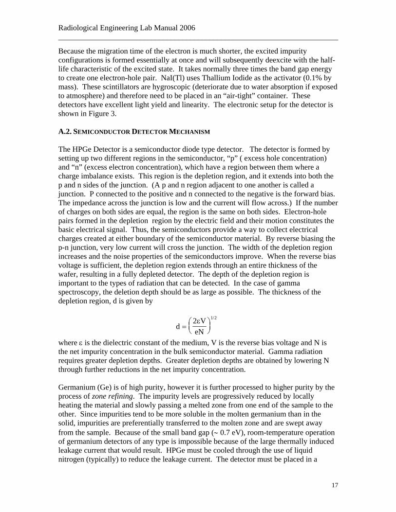
Because the migration time of the electron is much shorter, the excited impurity configurations is formed essentially at once and will subsequently deexcite with the half-life characteristic of the excited state. It takes normally three times the band gap energy to create one electron-hole pair. NaI(Tl) uses Thallium Iodide as the activator (0.1% by mass). These scintillators are hygroscopic (deteriorate due to water absorption if exposed to atmosphere) and therefore need to be placed in an “air-tight” container. These detectors have excellent light yield and linearity. The electronic setup for the detector is shown in Figure 3. A.2. SEMICONDUCTOR DETECTOR MECHANISM The HPGe Detector is a semiconductor diode type detector. The detector is formed by setting up two different regions in the semiconductor, “p” ( excess hole concentration) and “n” (excess electron concentration), which have a region between them where a charge imbalance exists. This region is the depletion region, and it extends into both the p and n sides of the junction. (A p and n region adjacent to one another is called a junction. P connected to the positive and n connected to the negative is the forward bias. The impedance across the junction is low and the current will flow across.) If the number of charges on both sides are equal, the region is the same on both sides. Electron-hole pairs formed in the depletion region by the electric field and their motion constitutes the basic electrical signal. Thus, the semiconductors provide a way to collect electrical charges created at either boundary of the semiconductor material. By reverse biasing the p-n junction, very low current will cross the junction. The width of the depletion region increases and the noise properties of the semiconductors improve. When the reverse bias voltage is sufficient, the depletion region extends through an entire thickness of the wafer, resulting in a fully depleted detector. The depth of the depletion region is important to the types of radiation that can be detected. In the case of gamma spectroscopy, the deletion depth should be as large as possible. The thickness of the depletion region, d is given by
dV
eN=
⎛⎝⎜
⎞⎠⎟
2 1 2ε /
where ε is the dielectric constant of the medium, V is the reverse bias voltage and N is the net impurity concentration in the bulk semiconductor material. Gamma radiation requires greater depletion depths. Greater depletion depths are obtained by lowering N through further reductions in the net impurity concentration. Germanium (Ge) is of high purity, however it is further processed to higher purity by the process of zone refining. The impurity levels are progressively reduced by locally heating the material and slowly passing a melted zone from one end of the sample to the other. Since impurities tend to be more soluble in the molten germanium than in the solid, impurities are preferentially transferred to the molten zone and are swept away from the sample. Because of the small band gap (∼ 0.7 eV), room-temperature operation of germanium detectors of any type is impossible because of the large thermally induced leakage current that would result. HPGe must be cooled through the use of liquid nitrogen (typically) to reduce the leakage current. The detector must be placed in a
17
Radiological Engineering Lab Manual 2006 ________________________________________________________________________
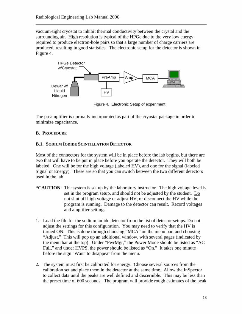
vacuum-tight cryostat to inhibit thermal conductivity between the crystal and the surrounding air. High resolution is typical of the HPGe due to the very low energy required to produce electron-hole pairs so that a large number of charge carriers are produced, resulting in good statistics. The electronic setup for the detector is shown in Figure 4.
PreAmp Amp
HV
MCA
Figure 4. Electronic Setup of experiment
Dewar w/Liquid
Nitrogen
HPGe Detectorw/Cryostat
The preamplifier is normally incorporated as part of the cryostat package in order to minimize capacitance. B. PROCEDURE B.1. SODIUM IODIDE SCINTILLATION DETECTOR
Most of the connectors for the system will be in place before the lab begins, but there are two that will have to be put in place before you operate the detector. They will both be labeled. One will be for the high voltage (labeled HV), and one for the signal (labeled Signal or Energy). These are so that you can switch between the two different detectors used in the lab. *CAUTION: The system is set up by the laboratory instructor. The high voltage level is
set in the program setup, and should not be adjusted by the student. Do not shut off high voltage or adjust HV, or disconnect the HV while the program is running. Damage to the detector can result. Record voltages and amplifier settings.
1. Load the file for the sodium iodide detector from the list of detector setups. Do not
adjust the settings for this configuration. You may need to verify that the HV is turned ON. This is done through choosing “MCA” on the menu bar, and choosing “Adjust.” This will pop up an additional window, with several pages (indicated by the menu bar at the top). Under “PwrMgr,” the Power Mode should be listed as “AC Full,” and under HVPS, the power should be listed as “On.” It takes one minute before the sign "Wait" to disappear from the menu.
2. The system must first be calibrated for energy. Choose several sources from the calibration set and place them in the detector at the same time. Allow the InSpector to collect data until the peaks are well defined and discernible. This may be less than the preset time of 600 seconds. The program will provide rough estimates of the peak
18
Radiological Engineering Lab Manual 2006 ________________________________________________________________________
energies. That estimate and relative positions should allow you to determine which peak corresponds to which gamma ray energy. In the Calibration menu, choose "Calibration by Energy only." Choose the energy with the cursor by placing the cursor at the top of the peak, and input the energy. Do this for all the energies that you can determine, and run the calibration. Use "Show" to check for linearity of the calibration curve before accepting the energy calibration. Use "Save As" under the "File" to save the spectrum to the computer.
3. Plot the gamma energy vs. channel # for all peaks used for energy calibration. 4. Remove all sources from the detector and clear the spectrum from the screen (be sure
you have saved it already). The next step is to measure the background from the detector. Allow the detector to collect data for at least twice as long as was taken in step two, and not less than two minutes (120 seconds). Note the total live time, and save this spectrum to another file. You will use it later.
5. Place the Cs-137 source back in the detector and collect a spectrum as in step two. 6. Under the “Options” menu, choose “Strip.” This will strip the background from the
spectroscopy results. Choose the file that you saved the background spectrum to. At the top of the window, there will be a place to enter a multiplication factor for the file. Correct the background counts so that the background spectrum is normalized to the time that the current spectrum has been collected. After stripping, the spectrum contains only sample peak information.
7. Determination of Peak Area. The Peak Area is the total counts under the full-energy
gamma-ray peak (or the photopeak) and is established by defining the Region of Interest (ROI ). The left and right bounds of the ROI can be moved by dragging them from the sides of the display, or by use of the CTRL-L and CTRL-R keys. Information of the ROI is summarized at the bottom of the screen. After the background stripping, the photopeaks are often still superimposed on a continuum that is caused by interactions of the gamma-rays with the detector. The counts shown as "Area" is the "peak area" without the continuum, and the counts shown as "Integral" include the continuum under the peak.
8. The system is now ready to be calibrated for counting efficiency. This is done by
dividing the peak area (without the continuum) with the activity of that sample, i.e.,
Efficiency (E) % = (Peak Area in Counts per Second)/(Sample Activity). Perform efficiency calibration for all photopeaks. The original activities of the standards and half-lives are used to determine the Sample Activity. Plot the counting efficiency (%) vs. gamma-ray energy in MeV. NaI detectors have better counting efficiencies (~ 5-10%) than the HPGe detectors (~0.1-1%).
19
Radiological Engineering Lab Manual 2006 ________________________________________________________________________
7. Energy Resolution of a system is determined by the width of a photopeak. Using the Cs-137 photopeak, the energy resolution is given by:
Energy Resolution (%) =(FWHM in keV)/(Peak Energy in keV),
Where FWHM = Full width of peak at half of the maximum peak height. NaI
detectors have worth energy resolutions than HPGe detectors. 8. Repeat step 6 only using the other standard sources provided to you, for all the photopeaks that you can identify (you may choose to put more than one standard in the detector at a time). B.2. HIGH PURITY GERMANIUM (HPGE)DETECTORS
CAUTION: The system is set up by the laboratory instructor. The high voltage level is set in the program setup, and should not be adjusted by the student. Do not shut off high voltage or adjust HV, or disconnect the HV while the program is running. Damage to the detector can result. NOTE: When placing the samples in front of the HPGe detector window, it is desirable to use a reproducible geometry (i.e., place each source in the same location) in order to generate meaningful results. 1. Close the detector file that was active. Disconnect the High Voltage and Signal
connectors from the Sodium Iodide detector and replace them from the ones from the High Purity Germanium Detector. Load the detector file for HPGe detector.
2. Perform energy calibrate for the system using the same procedures as described above.
3. Determine the energy at the peak channels on the calibrated system. Graph energy vs. channel no. for these points.
4. Measure background for the instrument and perform counting efficiency calibration for the system. Plot counting efficiency (%) vs. gamma energy (MeV).
6. Determine the energy resolution using Cs-137. Compare with result for NaI detector. 7. Verify characteristic peaks for various isotopes (Co-60, Cs-137 and Ba-133 standards). REPORT Printouts of the data collection may be made from the computer. It might be useful to have printouts of the different detector operations for use in your data analysis and your discussion. Make sure to answer all the questions in the narrative.
20
Radiological Engineering Lab Manual 2006 ________________________________________________________________________
Gamma-rays are uncharged and thus create no direct ionization or excitation of the material through which it traverses. The detection of gamma rays is critically dependent on interactions to cause the gamma-ray photon to transfer energy to an electron in the absorbing material. Gamma rays are also very penetrating. The Thallium-activated Sodium Iodide -NaI(Tl) is based on scintillation principles whereas the High Purity Germanium detector is based upon semiconductor principles. Discuss the detector principles and detector set-up (from when a photon enters the detector to a signal on the computer-channel accumulation). Discuss energy resolution (the separation of closely spaced gamma-rays), channels number vs. distinction between various peaks, the advantages disadvantages of the two detection (photopeak efficiencies, etc.). Compare and contrast the use of these two different instruments in the field of health physics. When and why would you choose one over the other?
21

Radiological Engineering Lab Manual 2006 ________________________________________________________________________
LAB #4 APPLICATION OF COMPUTER CODES FOR RISK
ASSESSMENT INVOLVING RELEASE OF RADIOACTIVE MATERIALS INTO THE ENVIRONMENT
OBJECTIVES: To familiarize the student with the use of available risk analysis software
in hypothetical real-world situations. REFERENCE: Class handout “Introduction to Health Physics”, Herman Cember, 3rd Ed. (1996). A. INTRODUCTION There are several reasons that someone in the field of Health Physics will want to model the effects of radiation release to the environment. One of the primary ones is to show compliance with the regulations set out by agencies such as the EPA and the NRC. The two codes used in this lab are made specifically for that purpose. The exercises in this experiment are practical examples of the use of risk analysis codes in the field of Health Physics. In the assignment, you are placed in a role as a health physicist, and are given information about a situation. You should complete the run of the risk analysis code and answer the questions that are part of the assignment, but your report should also include information about the codes themselves and how they are useful as tools in the field of health physics. This experiment uses the computer code CAP88PC version 2.1. It is installed on the computer in the NES classroom, but you may find it easier to use it on your own computer. It can be found at http://www.epa.gov/radiation/assessment/docs/ cap88pc211a.zip. If the code has difficulty locating the WND files, they should be moved into the main directory with the code executables (they are initially installed in the WND directory). B. EXERCISE 1 B.1. INTRODUCTION You are a corporate health physicist in charge of making does estimates; you have been tasked by a manufacturer of radiopharmaceuticals to evaluate three possible sites for locating a new facility. The three sites are 1). Boston, 2). Spokane, and 3). Providence; the atmospheric emission for the proposed facility are listed below in Table 1.
Table 1 Radionuclide Release (Ci/yr)
I-125 2.5 I-131 3.9 H-3 98 C-14 8.5 P-32 0.016
22
Radiological Engineering Lab Manual 2006 ________________________________________________________________________
Using the CAP88PC computer code, estimate the effective dose equivalent from the atmospheric emissions from each proposed site. Atmospheric emissions are through a single stack, however, the stack is not 2.5 times the building height so treat it as a ground release. B.2. DATA AND ASSUMPTIONS
Site information Boston, MA Spokane, WA Providence, RI Wind File BOS0211.WND GEG0360.WND PVD0560.WND Distance to receptor 300 m 330 m 350 m Annual Rainfall 108 cm 42 cm 118 cm Ambient Temperature 11 oC 9 oC 10 oC Lid Height 1000 m 1000 m 1000 m Food Scenario Urban Rural Urban Initial Stack Height 10 m 10 m 10 m Stack Diameter .2 m .2 m .2 m Stack Exit Velocity 10 m/s 10 m/s 10 m/s B.3. PROCEDURE
1. Estimate the dose from the atmospheric emissions for each site.
A. Start the program from the CAP88PC icon. To begin a new problem, you will need to create a new dataset
B. Once a dataset is created, all of the data pages are selected from the tabs at the top of the window.
C. In the Run Menu, select everything but the Chi/Q table. D. For values not otherwise provided, use the default values from CAP88PC E. Once all data fields are filled, save the dataset, and then execute it. F. The output of the code is put into the “OUTPUT” directory. They are labeled
with letters (not the chosen file name). They can be opened with any text editor. If you keep the same input file name, a new execution will overwrite the output files.
G. Create datasets for the remaining sites. Ensure you give each file a unique name since you will be using these files numerous times.
2. For each of the three sites, the effective dose equivalent is greater than 25 mrem/yr.
What stack height will yield an effective dose equivalent of 25 mrem/yr for the site with the lowest effective equivalent dose from part 1? Save the new data with a unique filename. It may take a couple of iterations to arrive at the correct height.
Stack Height:______ What stack height is required to obtain an effective dose equivalent of 25 mrem/yr at the Spokane site?
23
Radiological Engineering Lab Manual 2006 ________________________________________________________________________
Stack Height:______
3. When the company examines the results of your study, they determine that you have not collected adequate data on lid height. Furthermore they believe that the CAP88PC program is flawed because of the lack of lid height data. To respond to this criticism you perform a sensitivity analysis to determine how important lid height is in this study. You select three lid heights to evaluate: (1) 1000m, (2) 50% lower, and (3) 50% higher. Use the site and stack data from question 2.
How much impact did lid height have on the dose estimate?
4. In addition to the above, the company decides to install an evaporation pond (Area
source) into which liquid containing 50 Ci of H-3 will be discharged per year. They task you with determining the effective dose equivalent from this H-3, assuming all H-3 discharged evaporates. The pond will have an area of 2,200 m2. A. Use the site that yielded the lowest effective dose equivalent. In the site
parameters screen change the source field to “AREA” and enter the correct area B. In the release rate screen, delete all nuclides, except for H-3, and enter 50 Ci/yr as
the release rate.
What dose results from the evaporation of the H-3 from the pond? B.4. Results 1a. Which site yields the highest effective dose equivalent? 1b. Which site yields the lowest effective dose equivalent? For this site, which organ received the highest dose? C. EXERCISE 2 – POPULATION EXPOSURES
C.1. INTRODUCTION You are the environmental health physicist in charge of making dose estimates for the possible installation of a High Level Waste Tank Farm project at the KAPL Kesslering site. Your responsibility is to assess the effect on the surrounding population from this project. The project involves the installation of a set of tanks where high-level liquid waste is stored temporarily before being processed. The project would install four 500,000 gal tanks, secondary containment structures, and supporting systems. Normal environmental releases of radionuclides will occur from the new vessel off gas (VOG) system, via a proposed new stack. The effluent source term from the new stack is based on the release of radionuclides to the VOG system from volatilization of radioiodine and tritiated water vapor, as well as entrainment of nonvolatile radionuclides in liquid droplets.
24

Radiological Engineering Lab Manual 2006 ________________________________________________________________________
Nuclide Unfiltered
Release Rate (Ci/yr)
Total NCRP Screening Factor (Sv-m3/Bq)
H-3 3.59E+02 1.80E-06 Sr-90 2.52E+01 2.40E-01 Y-90 2.52E+01 2.10E-04 Zr-95 6.71E-01 4.00E-03
Nb-95 6.71E-01 1.20E-03 Ru-106 3.36E+00 8.00E-03 Sb-125 8.39E-01 1.60E-02
I-129 7.03E-01 3.20E-01 Cs-134 1.68E+01 1.20E-01 Cs-137 2.52E+01 1.70E-01 Ce-144 3.36E+01 4.00E-03 Pm-147 1.68E+01 2.40E-04 Eu-152 5.03E-03 1.40E-01 Eu-154 8.39E-01 1.20E-01 Eu-155 4.19E-01 4.60E-03 Pu-238 8.39E-02 1.30E+00 Pu-239 5.87E-04 1.40E+00 Pu-240 4.19E-04 1.40E+00 Pu-241 5.87E-02 2.70E-02
Am-241 3.36E-04 1.40E+00 C.2. DATA AND ASSUMPTIONS
1. Use conventional units (Ci and rem) 2. The population distribution is still reasonably close to the one contained in the
population file Kplkslrg.pop 3. The wind characteristics are similar to the Albany weather station data in
ALB0523.wnd 4. Assume the MEI eats contaminated leafy vegetables, produce, meat, and milk; but
drinks no contaminated water. Also assume the MEI eats no uncontaminated food.
5. Saratoga County follows a rural agricultural model. 6. Assume release is from a 65 m stack (point source) that has a diameter of 1.5 m
and an exit velocity of 20 m/s.
25
Radiological Engineering Lab Manual 2006 ________________________________________________________________________
C.3. PROCEDURE Use the above information to set up a new problem with CAP88-PC. Since this is a population study, change the individual distance entry to population entry and choose the correct population file.
Which radionuclides have the greatest impact on dose? Which pathways are important for each of these radionuclides? What is the meaning of “population dose”? How would you incorporate this into your recommendations?
26
Radiological Engineering Lab Manual 2006 ________________________________________________________________________
LAB #5 RADIATION DETECTION WITH THERMO-LUMINESCENT
DOSIMETERS (TLDS) AND THE MOSFET DOSIMETER SYSTEM OBJECTIVES: (1) To examine and compare thermoluminescent (TL) material and MOSFETs as means of measuring radiation dose. (2) To determine calibration curve for gamma rays on thermoluminescent dosimeters. (3) To determine the calibration factor of MOSFET dosimeters, and to study the linearity of MOSFET dosimeters. REFERENCE:
1. Introduction to Health Physics, Cember H., 1996. 2. Introduction to Radiological Physics and Radiation Dosimetry, Attix, F.H., 1986. 3. Operator’s manual for the MOSFET AutoSenseTM system, Thomson & Nielsen
Ltd., 2002. EQUIPMENT REQUIRED:
1. AutoSenseTM system including four MOSFET dosimeters, bias supply, and read-out system
2. Cs-137 source 3. Ionization chambers 4. Portable survey meter 5. 30 LiF-100 chips 6. Harshaw Atlas TLD Counting System 7. Nitrogen Gas
INTRODUCTION: A. INTRODUCTION A.1. THERMOLUMINESCENT MATERIAL
Certain materials are known to be affected by exposure to radiation. Some
change in the material occurs that can be used as an indication of how much radiation was received. These materials are commonly used in radiation detection devices. As will be seen in future experiments, most of these detectors are too bulky and would not be practical for personal radiation monitoring. Thermoluminescent (TL) material can detect radiation and comes in a powder form or as small chips. This material can be put into a badge that can be used as a personal detector. These thermoluminescent detectors, or TLDs are the most commonly used personal monitoring devices.
Some material when exposed to radiation will promptly emit the energy imparted by the radiation. It is usually in the form of light and is used widely in radiation detectors. TL material will also emit the energy imparted in it by incident radiation, but it must be heated to do so.
27
Radiological Engineering Lab Manual 2006 ________________________________________________________________________
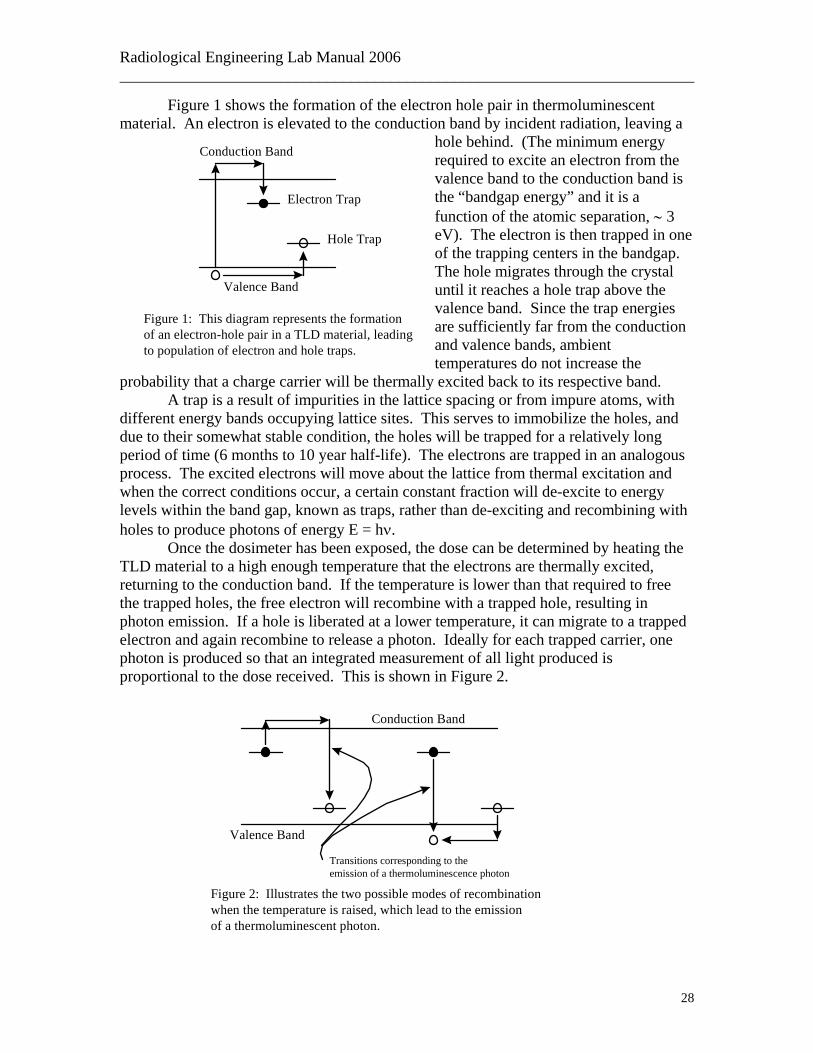
Figure 1 shows the formation of the electron hole pair in thermoluminescent material. An electron is elevated to the conduction band by incident radiation, leaving a
hole behind. (The minimum energy required to excite an electron from the valence band to the conduction band is the “bandgap energy” and it is a function of the atomic separation, ∼ 3 eV). The electron is then trapped in one of the trapping centers in the bandgap. The hole migrates through the crystal until it reaches a hole trap above the valence band. Since the trap energies are sufficiently far from the conduction and valence bands, ambient temperatures do not increase the
probability that a charge carrier will be thermally excited back to its respective band.
Conduction Band
Valence Band
Electron Trap
Hole Trap
Figure 1: This diagram represents the formationof an electron-hole pair in a TLD material, leadingto population of electron and hole traps.
A trap is a result of impurities in the lattice spacing or from impure atoms, with different energy bands occupying lattice sites. This serves to immobilize the holes, and due to their somewhat stable condition, the holes will be trapped for a relatively long period of time (6 months to 10 year half-life). The electrons are trapped in an analogous process. The excited electrons will move about the lattice from thermal excitation and when the correct conditions occur, a certain constant fraction will de-excite to energy levels within the band gap, known as traps, rather than de-exciting and recombining with holes to produce photons of energy E = hν.
Once the dosimeter has been exposed, the dose can be determined by heating the TLD material to a high enough temperature that the electrons are thermally excited, returning to the conduction band. If the temperature is lower than that required to free the trapped holes, the free electron will recombine with a trapped hole, resulting in photon emission. If a hole is liberated at a lower temperature, it can migrate to a trapped electron and again recombine to release a photon. Ideally for each trapped carrier, one photon is produced so that an integrated measurement of all light produced is proportional to the dose received. This is shown in Figure 2.
Transitions corresponding to theemission of a thermoluminescence photon
Figure 2: Illustrates the two possible modes of recombinationwhen the temperature is raised, which lead to the emissionof a thermoluminescent photon.
Conduction Band
Valence Band
28
Radiological Engineering Lab Manual 2006 ________________________________________________________________________
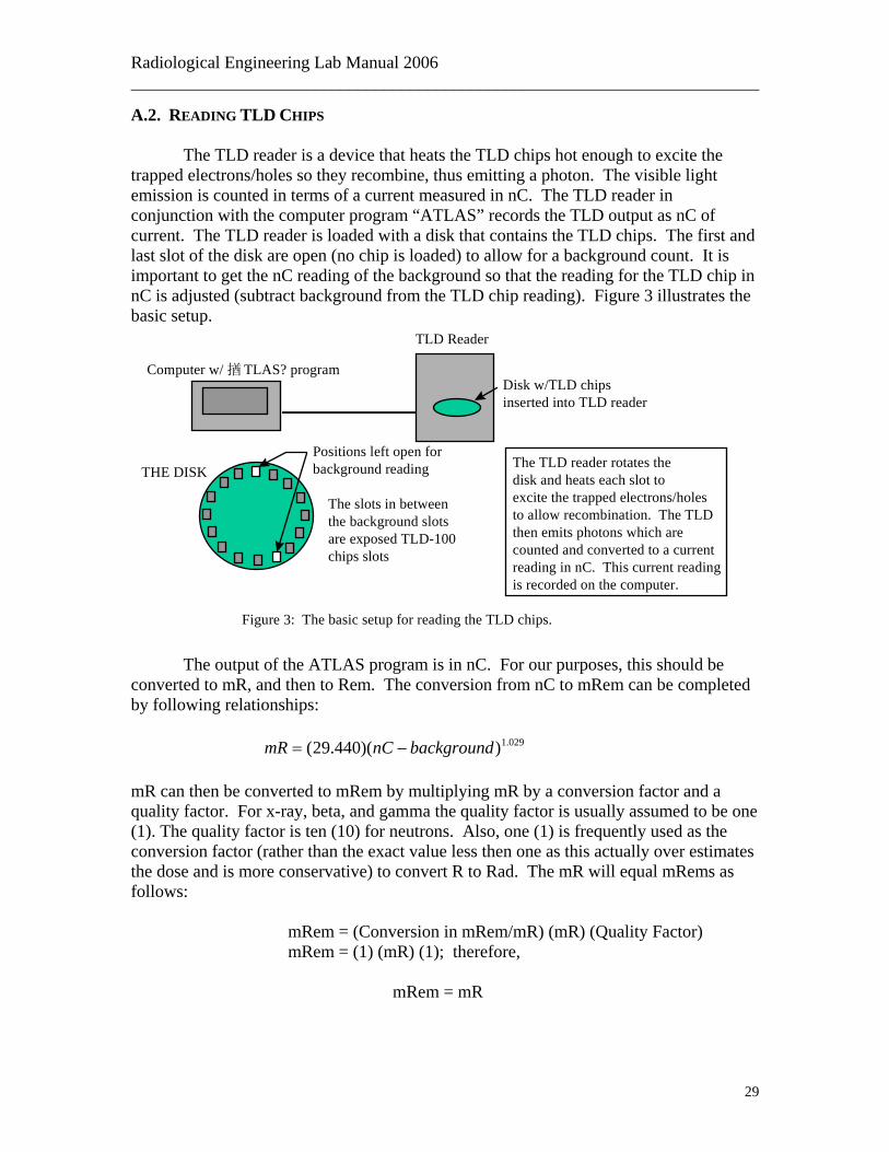
A.2. READING TLD CHIPS The TLD reader is a device that heats the TLD chips hot enough to excite the trapped electrons/holes so they recombine, thus emitting a photon. The visible light emission is counted in terms of a current measured in nC. The TLD reader in conjunction with the computer program “ATLAS” records the TLD output as nC of current. The TLD reader is loaded with a disk that contains the TLD chips. The first and last slot of the disk are open (no chip is loaded) to allow for a background count. It is important to get the nC reading of the background so that the reading for the TLD chip in nC is adjusted (subtract background from the TLD chip reading). Figure 3 illustrates the basic setup.
TLD Reader
Computer w/ 揂TLAS? programDisk w/TLD chipsinserted into TLD reader
Positions left open forbackground reading
The slots in betweenthe background slotsare exposed TLD-100chips slots
THE DISKThe TLD reader rotates thedisk and heats each slot toexcite the trapped electrons/holesto allow recombination. The TLDthen emits photons which arecounted and converted to a currentreading in nC. This current readingis recorded on the computer.
Figure 3: The basic setup for reading the TLD chips.
The output of the ATLAS program is in nC. For our purposes, this should be converted to mR, and then to Rem. The conversion from nC to mRem can be completed by following relationships:
029.1))(440.29( backgroundnCmR −= mR can then be converted to mRem by multiplying mR by a conversion factor and a quality factor. For x-ray, beta, and gamma the quality factor is usually assumed to be one (1). The quality factor is ten (10) for neutrons. Also, one (1) is frequently used as the conversion factor (rather than the exact value less then one as this actually over estimates the dose and is more conservative) to convert R to Rad. The mR will equal mRems as follows: mRem = (Conversion in mRem/mR) (mR) (Quality Factor) mRem = (1) (mR) (1); therefore,
mRem = mR
29
Radiological Engineering Lab Manual 2006 ________________________________________________________________________
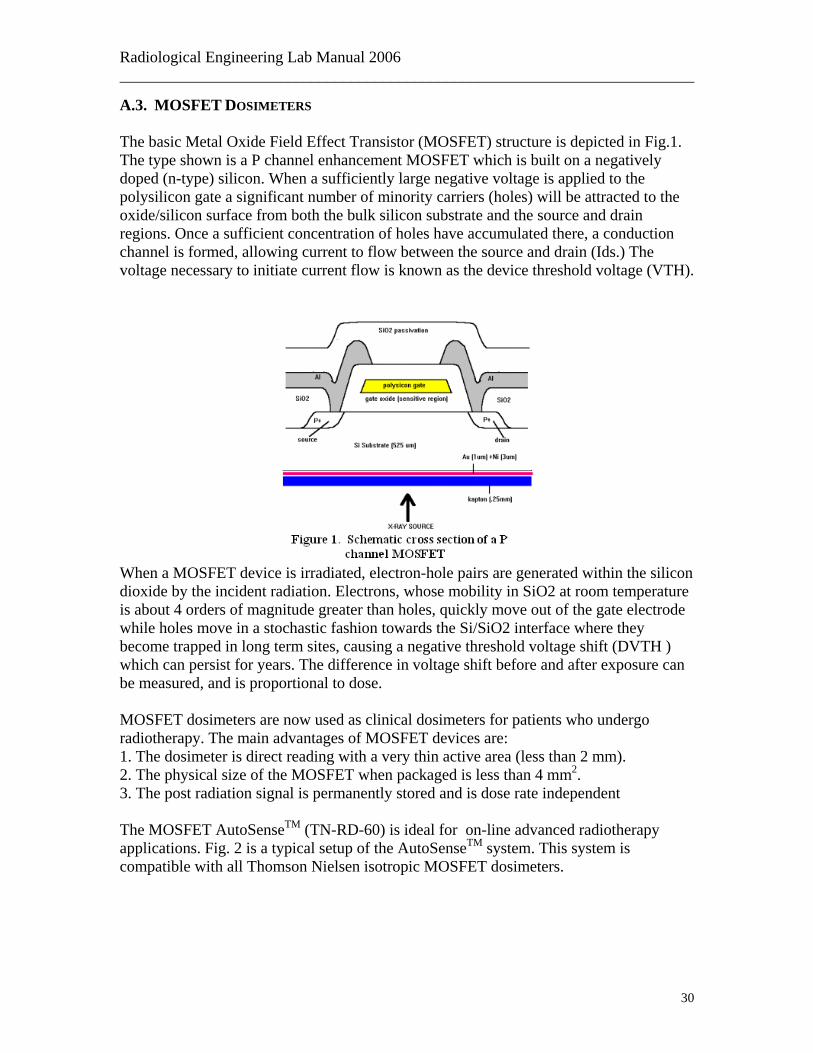
A.3. MOSFET DOSIMETERS The basic Metal Oxide Field Effect Transistor (MOSFET) structure is depicted in Fig.1. The type shown is a P channel enhancement MOSFET which is built on a negatively doped (n-type) silicon. When a sufficiently large negative voltage is applied to the polysilicon gate a significant number of minority carriers (holes) will be attracted to the oxide/silicon surface from both the bulk silicon substrate and the source and drain regions. Once a sufficient concentration of holes have accumulated there, a conduction channel is formed, allowing current to flow between the source and drain (Ids.) The voltage necessary to initiate current flow is known as the device threshold voltage (VTH).
When a MOSFET device is irradiated, electron-hole pairs are generated within the silicon dioxide by the incident radiation. Electrons, whose mobility in SiO2 at room temperature is about 4 orders of magnitude greater than holes, quickly move out of the gate electrode while holes move in a stochastic fashion towards the Si/SiO2 interface where they become trapped in long term sites, causing a negative threshold voltage shift (DVTH ) which can persist for years. The difference in voltage shift before and after exposure can be measured, and is proportional to dose. MOSFET dosimeters are now used as clinical dosimeters for patients who undergo radiotherapy. The main advantages of MOSFET devices are: 1. The dosimeter is direct reading with a very thin active area (less than 2 mm). 2. The physical size of the MOSFET when packaged is less than 4 mm2. 3. The post radiation signal is permanently stored and is dose rate independent The MOSFET AutoSenseTM (TN-RD-60) is ideal for on-line advanced radiotherapy applications. Fig. 2 is a typical setup of the AutoSenseTM system. This system is compatible with all Thomson Nielsen isotropic MOSFET dosimeters.
30
Radiological Engineering Lab Manual 2006 ________________________________________________________________________
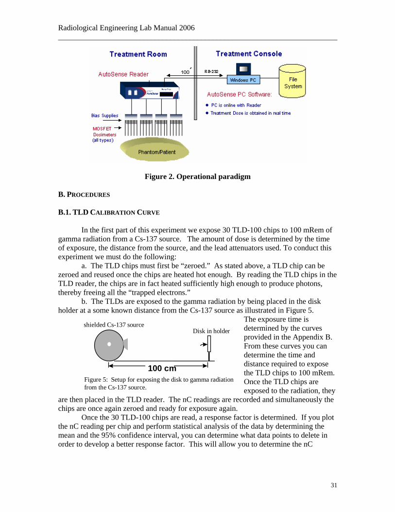
Figure 2. Operational paradigm
B. PROCEDURES B.1. TLD CALIBRATION CURVE In the first part of this experiment we expose 30 TLD-100 chips to 100 mRem of gamma radiation from a Cs-137 source. The amount of dose is determined by the time of exposure, the distance from the source, and the lead attenuators used. To conduct this experiment we must do the following:
a. The TLD chips must first be “zeroed.” As stated above, a TLD chip can be zeroed and reused once the chips are heated hot enough. By reading the TLD chips in the TLD reader, the chips are in fact heated sufficiently high enough to produce photons, thereby freeing all the “trapped electrons.”
b. The TLDs are exposed to the gamma radiation by being placed in the disk holder at a some known distance from the Cs-137 source as illustrated in Figure 5.
The exposure time is determined by the curves provided in the Appendix B. From these curves you can determine the time and distance required to expose the TLD chips to 100 mRem. Once the TLD chips are exposed to the radiation, they
are then placed in the TLD reader. The nC readings are recorded and simultaneously the chips are once again zeroed and ready for exposure again.
100 cm
shielded Cs-137 sourceDisk in holder
Figure 5: Setup for exposing the disk to gamma radiationfrom the Cs-137 source.
Once the 30 TLD-100 chips are read, a response factor is determined. If you plot the nC reading per chip and perform statistical analysis of the data by determining the mean and the 95% confidence interval, you can determine what data points to delete in order to develop a better response factor. This will allow you to determine the nC
31
Radiological Engineering Lab Manual 2006 ________________________________________________________________________
reading for a 100 mRem exposure. This ratio should provide a response factor in terms of mRem/nC. The thermoluminescent material used will be natural LiF, TLD-100.
1. Read carefully Appendix A which details the procedure for utilizing the Atlas
TLD reader system.
2. You will be given 30 TLD chips (Make sure you don’t drop them inadvertently!).
3. Each chip must be “zeroed” by reading them in the TLD reader. The reading process involves heating the TL material, which as discussed produces photons thereby freeing all the “trapped electrons”, and eliminates any record of the previous exposure.
4. After the chips are “zeroed,” the Cs-137 source will be utilized to expose the TLD
material for predetermined dose in mR. The amount of dose is controlled by the time of exposure.
5. Expose all TLD’s to 100mR to determine whether or not all the chips have
uniform response. The exposure will be made at some known distance and work with the lab instructor to determine the time of exposure. Read the chips in the same way you zeroed them, but keep the reading results. Plot and compare the readings of the chips. Chips with too low or too high a response should not be used further.
6. Now you need to determine the calibration curve for the TLD reader. A
calibration curve allow others to calculate the exposure in mR from a reading in nC. The calibration curve should be valid for a wide range of exposures. Divide the good chips into five groups. These groups will be exposed to doses of 25, 50, 100, 250, and 500 mR, respectively, at 50 cm distance from source without lead shielding present. Work with the instructor to determine the exposure time.
Suggestion: Each lab group member at this time should pick a set (or sets) of chips and follow these through the whole lab, in order to get a chance to perform each of the required tasks.
7. Once chips have been exposed to different doses, you can read them again. Plot
the results (mR versus nC) and calculate the calibration curve by using a least squares fit to the data with 95% confidence level. This curve should not be too different from the one given in the Appendix.
Use the calibration curve you have calculated to determine the following:
1. Mean of the readings for each group in mR. 2. Standard deviation in mR (error propagated from nC) for each group. 3. Range of the readings for each group.
32
Radiological Engineering Lab Manual 2006 ________________________________________________________________________
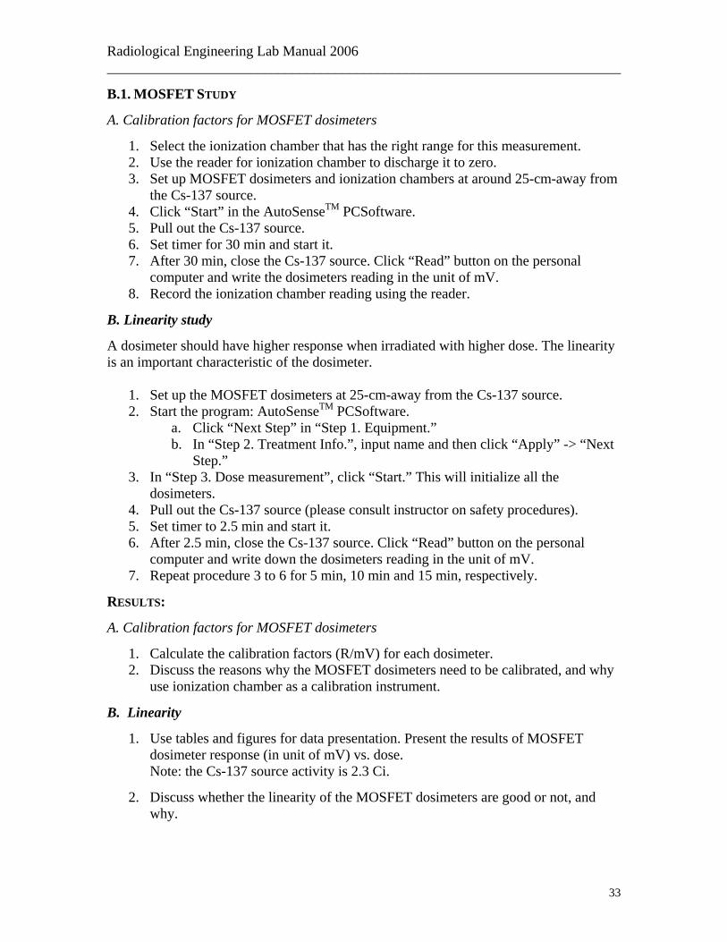
B.1. MOSFET STUDY
A. Calibration factors for MOSFET dosimeters
1. Select the ionization chamber that has the right range for this measurement. 2. Use the reader for ionization chamber to discharge it to zero. 3. Set up MOSFET dosimeters and ionization chambers at around 25-cm-away from
the Cs-137 source. 4. Click “Start” in the AutoSenseTM PCSoftware. 5. Pull out the Cs-137 source. 6. Set timer for 30 min and start it. 7. After 30 min, close the Cs-137 source. Click “Read” button on the personal
computer and write the dosimeters reading in the unit of mV. 8. Record the ionization chamber reading using the reader.
B. Linearity study
A dosimeter should have higher response when irradiated with higher dose. The linearity is an important characteristic of the dosimeter.
1. Set up the MOSFET dosimeters at 25-cm-away from the Cs-137 source. 2. Start the program: AutoSenseTM PCSoftware.
a. Click “Next Step” in “Step 1. Equipment.” b. In “Step 2. Treatment Info.”, input name and then click “Apply” -> “Next
Step.” 3. In “Step 3. Dose measurement”, click “Start.” This will initialize all the
dosimeters. 4. Pull out the Cs-137 source (please consult instructor on safety procedures). 5. Set timer to 2.5 min and start it. 6. After 2.5 min, close the Cs-137 source. Click “Read” button on the personal
computer and write down the dosimeters reading in the unit of mV. 7. Repeat procedure 3 to 6 for 5 min, 10 min and 15 min, respectively.
RESULTS:
A. Calibration factors for MOSFET dosimeters
1. Calculate the calibration factors (R/mV) for each dosimeter. 2. Discuss the reasons why the MOSFET dosimeters need to be calibrated, and why
use ionization chamber as a calibration instrument.
B. Linearity
1. Use tables and figures for data presentation. Present the results of MOSFET dosimeter response (in unit of mV) vs. dose. Note: the Cs-137 source activity is 2.3 Ci.
2. Discuss whether the linearity of the MOSFET dosimeters are good or not, and why.
33
Radiological Engineering Lab Manual 2006 ________________________________________________________________________
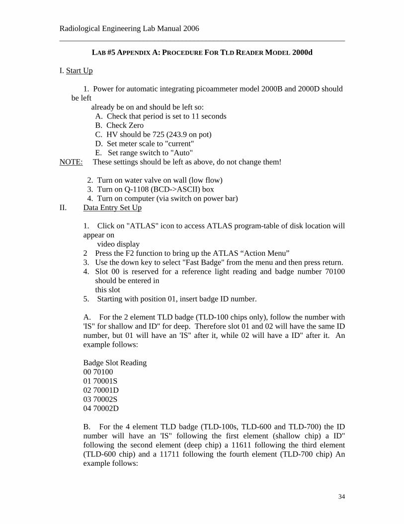
LAB #5 APPENDIX A: PROCEDURE FOR TLD READER MODEL 2000d I. Start Up 1. Power for automatic integrating picoammeter model 2000B and 2000D should
be left already be on and should be left so:
A. Check that period is set to 11 seconds B. Check Zero C. HV should be 725 (243.9 on pot) D. Set meter scale to "current" E. Set range switch to "Auto" NOTE: These settings should be left as above, do not change them! 2. Turn on water valve on wall (low flow) 3. Turn on Q-1108 (BCD->ASCII) box 4. Turn on computer (via switch on power bar) II. Data Entry Set Up
1. Click on "ATLAS" icon to access ATLAS program-table of disk location will appear on video display 2 Press the F2 function to bring up the ATLAS “Action Menu” 3. Use the down key to select "Fast Badge" from the menu and then press return. 4. Slot 00 is reserved for a reference light reading and badge number 70100
should be entered in this slot
5. Starting with position 01, insert badge ID number.
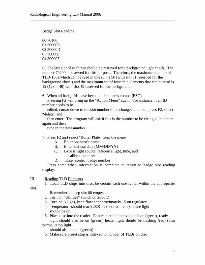
A. For the 2 element TLD badge (TLD-100 chips only), follow the number with 'IS" for shallow and ID" for deep. Therefore slot 01 and 02 will have the same ID number, but 01 will have an 'IS" after it, while 02 will have a ID" after it. An example follows:
Badge Slot Reading 00 70100 01 70001S 02 70001D 03 70002S 04 70002D
B. For the 4 element TLD badge (TLD-100s, TLD-600 and TLD-700) the ID number will have an 'IS" following the first element (shallow chip) a ID" following the second element (deep chip) a 11611 following the third element (TLD-600 chip) and a 11711 following the fourth element (TLD-700 chip) An example follows:
34
Radiological Engineering Lab Manual 2006 ________________________________________________________________________
Badge Slot Reading
00 70100 01 50000S 02 50000D 03 500006 04 500007 C. The last slot of each run should be reserved for a background light check. The number 70200 is reserved for this purpose. Therefore, the maximum number of TLD-100s which can be read in one run is 50 (with slot 51 reserved for the background check) and the maximum set of four chip elements that can be read is 12 (12x4=48) with slot 49 reserved for the background. 6. When all badge Ids have been entered, press escape (ESC). Pressing F2 will bring up the “Action Menu” again. For instance, if an ID number needs to be edited, cursor down to the slot number to be changed and then press F2, select “delete” and then enter. The program will ask if this is the number to be changed, hit enter again and then type in the new number.
7. Press F2 and select "Boiler Plate" from the menu
A. Enter operator's name B. Enter last use date (MM/DD/YY) C. Bypass light source, reference light, time, and
calibration curve D. Enter control badge number
Press enter when information is complete to return to badge slot reading display.
III. Reading TLD Elements 1. Load TLD chips into disc, be certain each one is flat within the appropriate slot. Remember to keep slot 00 empty. 2. Turn on "Utilities" switch on 2000 D 3. Turn on N2 gas, keep flow at approximately 15 on regulator 4. Temperature should reach 280C and normal temperature light
should be on. 5. Place disc into the reader. Ensure that the index light is on (green), ready
light should also be on (green), heater light should be flashing (red) (also normal temp light should also be on (green))
6. Make sure preset stop is indexed to number of TLDs on disc
35
Radiological Engineering Lab Manual 2006 ________________________________________________________________________
7. Make sure cover of reader is closed. DO NOT OPEN COVER DURING ANY READ CYCLE! 8. Press reference light and allow machine to take reading 9. At the computer, press F3 to place in receive mode. 10.Once the reference light value has been received on computer video display, press "Auto Start" button on 2000D to begin read cycle (REMEMBER NOT TO OPEN COVER DURING READ CYCLE-if necessary, stop machine by pressing "Stop" button on 2000D first) 11.Nanocoulomb readings will now be taken for each TLD element in the disc and reader. 12.After the completion of the read cycle make sure that only the red light on the "Stop" button is on ("Auto Start" light is off) before lifting the cover to remove disc with chips. 13.Press F2 to bring up menu. Select "Save Batch" if one desires to save the readings to the hard
drive. 14.Give file name and enter. Program will ask if these are Whole Body or Extremity readings. Select appropriate letter e.g., "WI' for whole body or "El' for extremity. 15.Program will also ask you to confirm the date last worn and control badge number. A 11
Save Complete" message should appear at the bottom of the video display. 16.Press "Print Screen" to print a hard copy of the readings
IV. Shut Down Procedures 1. Make sure disc is removed from reader. 2. Turn off N. gas, an alarm will sound, depress "alarm reset" on reader to turn
off. 3. Turn off "utilities" on reader. 4. Allow temperature to fall below 150C and then turn off water valve on the
wall 5. Turn off the Q-1108 (BCD->ASCII) box. 6. Leave power to 2000B and 2000D on 7. Escape from ATLAS program. 8. Click on "Windows" icon 9. Click on start up 10. Click on shut down 11. Follow prompts, when message indicates it is safe to turn off the computer do so by switch on power bar
36
Radiological Engineering Lab Manual 2006 ________________________________________________________________________
Note on Reading TLD Elements 1. During reading cycle, the screen saver may appear on the video display. To get back to the ATLAS program, click on left mouse button and then on "ATLAS" on the bottom scroll bar (not on the ATLAS icon as this will open a second ATLAS window.) 2. Be sure to save file first if desired before printing screen. Currently, one cannot get back to the program after printing and it is necessary to escape and then click on the "ATLAS" icon to get back to the program (boiler plate must be filled out again at this point as well).
Interpretation
1. The interpretation from nancoulombs to mrem can be completed by several calculations and it is not necessary to use the MTS program to do so (I would prefer not to have students working in this if possible). 2. Subtract background nanocoulomb from reading (calculate net nanocoulomb
reading) 3. Determine mR by plugging the previous value into empirically derived
equation. Currently for beta we are using the following:
mR=(31.4620)nC1.037.
For gamma we are currently using the following: mR=(29.440)nCl.029. 4. mR can be converted to mrem by multiplying mR by a conversion factor and a quality factor. For x-ray, beta and gamma the quality factor is usually assumed to be one (1) , it will be different for neutrons. One (1), is frequently used as the conversion factor (rather than the exact value less then one as this actually over estimates the dose and is more conservative). Therefore, mR will equal mrem as follows:
mRem=(Conversion in mRem/mR) (mR) (Quality Factor) mrem= (1) (mR) (1) ; therefore mRem=mR.
37

Radiological Engineering Lab Manual 2006 ________________________________________________________________________
LAB #6 RADIATION SURVEY AND CONTAMINATION CONTROL AT RPI
FACILITIES OBJECTIVES: This session provides the student with experience in making radiation
survey and contamination control in the vicinity of radiation sources REFERENCES: “Radiation Detection and Measurement”, by G.F. Knoll, 2nd Ed. (1989). “Introduction to Health Physics”, Herman Cember, 3nd Ed. (1996).
NYSHD Sanitary Code Part 16 EQUIPMENT REQUIRED:
1. Gamma Survey Instrument 2. Personnel Monitoring Device (TLD Badge) 3. Swipe papers (for proportional counter and/or liquid scintillation counter) 4. Tennelec Automatic Sample Changer and Planchets 5. Calibration Sources 6. Floor Maps of Gaerttner Laboratory, 25 Meter Experimental Room, or Blaw
Knox I Waste Storage Facility A. PROCEDURE Two different types of measurements will be made at a radiation facility on campus: 1) radiation levels measured with a portable survey meter, and 2) loose contamination levels measured by taking and counting swipe samples from floor or surface of the radiation sources. Depending on the contamination, the swipes will then be counted with proportional counter for high energy alpha/beta particles or by a liquid scintillation counter for low energy beta particles (such as C-14 and H-3). These surveys are performed each month by each radiation facility in order to demonstrate the compliance with regulations. CAUTION: When making radiation surveys of any kind, do not loiter in the Radiation Areas. Remember, radiation exposures should also be kept ALARA.
1) The survey meters used should be suitable for the radiation levels to be measured. Background radiation levels are as low as 30 µR/h, while a “Radiation Area” has a dose rate at least 5mR/h. One should test the meter and check for battery and calibration status. During the survey, the meter should be held at about 1 meter above the floor and about 30 cm from a known radiation source. Because a meter may be angular dependent and/or your body may shield the radiation, one should try to adjust the orientation until a maximum reading is obtained. Record the reading on the map for each location. When entering an unknown radiation area, set the meter scale to the highest and then change it to a lower one if the meter is not responding. Students are to work together during the measurements. One student making the measurements with the radiation survey meter and the other student recording the data. Both students should verify each reading. The floor plan should provide a useful guide on where readings and
38

Radiological Engineering Lab Manual 2006 ________________________________________________________________________
swipe samples should be taken. All radiation “Hot Spots” in a room should be identified and noted on the floor plan. Check for posted “Radiation Areas” sign if the dose rate is greater than 5mR/h at 30 cm from a source. 2) Each group of students will be provided with a set of swipes and holders. The swipes for high energy alpha/beta contamination are different from the ones used for low energy beta particles. It is important to know what type of contaminant might exist in a lab in advance by checking, for example, the radioactive material inventory. Number swipes according to the “Swipe Data Sheet” and the map. These swipes are used by wiping the cloth side over the surface to be checked. These type of contamination is called “loose” or “removable” contamination. The area to be “swiped” should be approximately 10 cm X 10 cm. These swipes should be made on floors, table tops, and equipment surface where the use of radioactive material might have caused contamination. Disposable gloves should be used to prevent cross contamination. The gloves are to be disposed of as radioactive waste if contaminated. When the swipes are completed, load the samples into the Tennelec proportional counter system and count them for both alpha and beta radioactivity. The swipes for low energy beta radioactivity are counted by the instructor using a liquid scintillation counter. Calculate the counting time by making sure that the Lower Limit of Detection is below the contamination limits (assuming the background counting rate is about 1 cpm and the counting efficiency for alpha is about 20%). Remeber LLD (in dpm/swipe)=[4.66x(backround counts)1/2 + 3]/[(counting time in min)x(counting eff.)]. You may pick up your results on the next day. Report your results in dpm/100 cm2. Compare surface contamination levels with New York State limits listed on the “Swipe Data Sheet.” B. REPORT Use tables and maps for data presentation. Discuss your findings and compare with the dose limits (provide a list of dose and contamination limits). How long an individual may stay in the area without exceeding these limits? Discuss the hot spots where contamination and/or high dose rate exists. Show your calculation for the LLD of the Tennelec system (What counting time do you recommend?).
39
Radiological Engineering Lab Manual 2006 ________________________________________________________________________
LAB #7 AIR SAMPLING FOR RADON
OBJECTIVES: To learn methods used for determining radon (Rn-222 and daughters)
concentration in air and compare the results against EPA recommendations.
REFERENCES: “Radiation Detection and Measurement”, by G.F. Knoll, 2nd Ed. (1989). “Introduction to Health Physics”, Herman Cember, 3rd Ed. (1996). EQUIPMENT REQUIRED:
• Gamma-spectroscopy system (NaI detector) • Calibration Kit for Air Samplers
A. INTRODUCTION
Radon comes from the natural decay of uranium. It can be found in high concentrations in soils and rocks containing uranium. One working level, WL, is a quantity used to quantify the radon concentration and is defined as the potential alpha energy emission of 1.3 x 10⁵ MeV with the complete decay of the short-lived daughter products of Rn-222 (i.e., Po-218, Pb-214, Bi-214, and Po-214) in one liter of air (see Fig. 1). If the short-lived progeny are in equilibrium with the 3.82 day half-life of Rn-222, then one WL corresponds to a Rn-222 concentration of 100 pCi/L. Radon is an alpha emitter, but because of its relatively long half-life and the fact that it is not collected in the lungs, its potential alpha contribution is usually negligible (5 percent) compared to the daughters. The equilibrium fraction (also called equilibrium factor or equilibrium ratio), which is a measure of the extent of dis-equilibrium between radon and progeny, is defined as:
F=[(# WL)(100 pCi)]/[Concentration of Rn 222 in pCi/L], and is often less than 1 for many exposure situations. A value of 0.5 has been generally assumed for control and assessment purposes when it is impractical to measure F. An exposure to radon at a concentration of 200 pCi/L with an equilibrium factor of 0.5 has the same dose impact as does an exposure for the same time interval to a concentration of 100 pCi/L when radon and progeny are in equilibrium. The EPA has established a value of 4 pCi/L in screening public exposure as a level at which follow-up measurements are justified. The EPA recommends the home to be fixed if the long-term averaged concentration is above 4 pCi/L. B. PROCEDURE For this method, an airtight container with activated charcoal is opened in the area to be sampled and radon in the air adsorbs onto the charcoal granules. At the end of the sampling (3 - 5 days), the container is sealed and sent to a laboratory for analysis.
1. Each group will be provided with several charcoal canisters exposed previously.
40

Radiological Engineering Lab Manual 2006 ________________________________________________________________________
2. Record information on location and time period from the cover of the canister. The canister should be counted as soon as possible. A decay correction may be applied if the time between sealing the canister and counting is too long.
3. Take a 10 min. (600 seconds) count for a blank canister (for background) and the sample canister using the 3x3 NaI detector.
4. The photopeaks from the radon daughters (Pb-214 at 0.242, 0.294, and 0.352 MeV and Bi-214 at 0.609 MeV) are of interest. Set the region of interest (ROI) from 220 keV to 380 keV, and determine the Gross Integral counts for both the background and the sample canister. The radon concentration is then calculated by: Radon Concent. (pCi/L) = [(Gross for sample)- (gross for blank)]/(CF), where CF is a calibration factor and is equal to 238 counts/pCi/L. If no decay correction is needed, this will be the radon concentration for the area measured.
5. Compare your results with EPA recommendations. Provide a remediation action plan if necessary
41
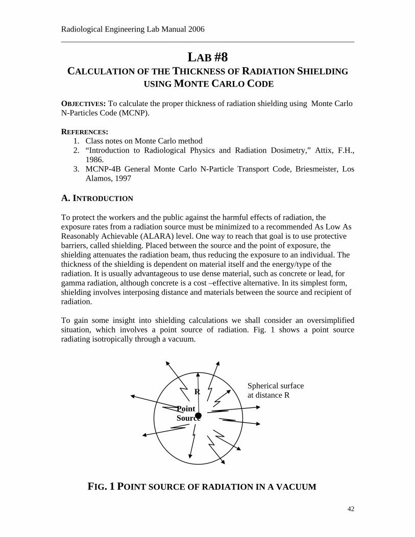
Radiological Engineering Lab Manual 2006 ________________________________________________________________________
LAB #8 CALCULATION OF THE THICKNESS OF RADIATION SHIELDING
USING MONTE CARLO CODE OBJECTIVES: To calculate the proper thickness of radiation shielding using Monte Carlo N-Particles Code (MCNP). REFERENCES:
1. Class notes on Monte Carlo method 2. “Introduction to Radiological Physics and Radiation Dosimetry,” Attix, F.H.,
1986. 3. MCNP-4B General Monte Carlo N-Particle Transport Code, Briesmeister, Los
Alamos, 1997 A. INTRODUCTION To protect the workers and the public against the harmful effects of radiation, the exposure rates from a radiation source must be minimized to a recommended As Low As Reasonably Achievable (ALARA) level. One way to reach that goal is to use protective barriers, called shielding. Placed between the source and the point of exposure, the shielding attenuates the radiation beam, thus reducing the exposure to an individual. The thickness of the shielding is dependent on material itself and the energy/type of the radiation. It is usually advantageous to use dense material, such as concrete or lead, for gamma radiation, although concrete is a cost –effective alternative. In its simplest form, shielding involves interposing distance and materials between the source and recipient of radiation. To gain some insight into shielding calculations we shall consider an oversimplified situation, which involves a point source of radiation. Fig. 1 shows a point source radiating isotropically through a vacuum.
Spherical surface at distance R
Point Source
R
FIG. 1 POINT SOURCE OF RADIATION IN A VACUUM
42

Radiological Engineering Lab Manual 2006 ________________________________________________________________________
According to the inverse square law, the intensity of radiation on the surface of a sphere of radius R will be:
2R4S
π=I (1)
Gamma Source
Pb Shield (Attenuator)
Detector
R
x
Figure 2: Pb Shield attenuates gamma radiation reaching the detector.
Where S is the source strength (number of particles or rays per unit time). If we place enough distance between ourselves and the source, the intensity of radiation will be reduced to safe levels. However, if we place material between ourselves and the source, we can take advantage of attenuation provided by the material. For the case of a collimated beam of gamma particles, the intensity at a point in the material will be:
R oI µ−= eI (2)
Where µ is the total linear absorption coefficient. Equation (2) applies strictly to a collimated beam and only when scattered radiation is removed from the beam. In a thicker shield such as that in Fig. 3, some of the radiation is backscattered into the path and Equation (2) has to be modified to include a Berger Build-up Factor, which makes the equation difficult to solve.
Source Figure 3: Backscattering of radiation in a shield
43
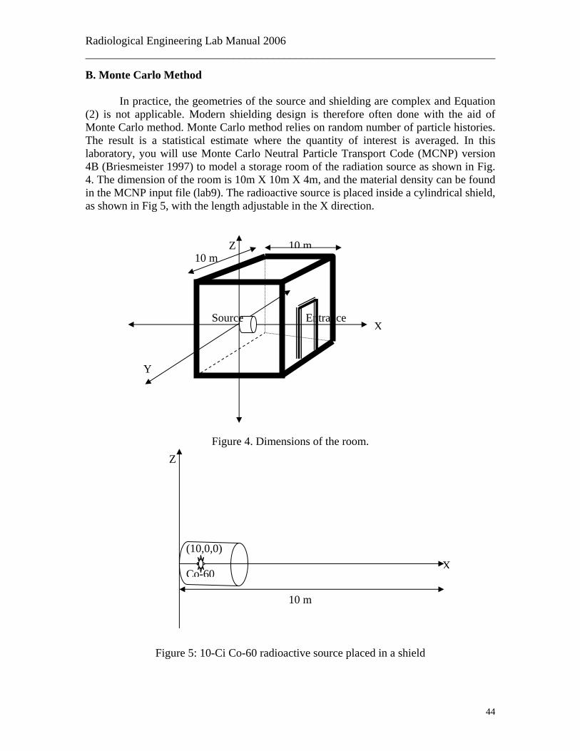
Radiological Engineering Lab Manual 2006 ________________________________________________________________________
B. Monte Carlo Method In practice, the geometries of the source and shielding are complex and Equation (2) is not applicable. Modern shielding design is therefore often done with the aid of Monte Carlo method. Monte Carlo method relies on random number of particle histories. The result is a statistical estimate where the quantity of interest is averaged. In this laboratory, you will use Monte Carlo Neutral Particle Transport Code (MCNP) version 4B (Briesmeister 1997) to model a storage room of the radiation source as shown in Fig. 4. The dimension of the room is 10m X 10m X 4m, and the material density can be found in the MCNP input file (lab9). The radioactive source is placed inside a cylindrical shield, as shown in Fig 5, with the length adjustable in the X direction.
Y
mZ 10 m
XSource Entrance
Figure 4. Dimensions of the room. Z
0
(10,0,0)
10 m
Figure 5: 10-Ci Co-60 radioactive source place
10
X
d in a shield
Co-6
44
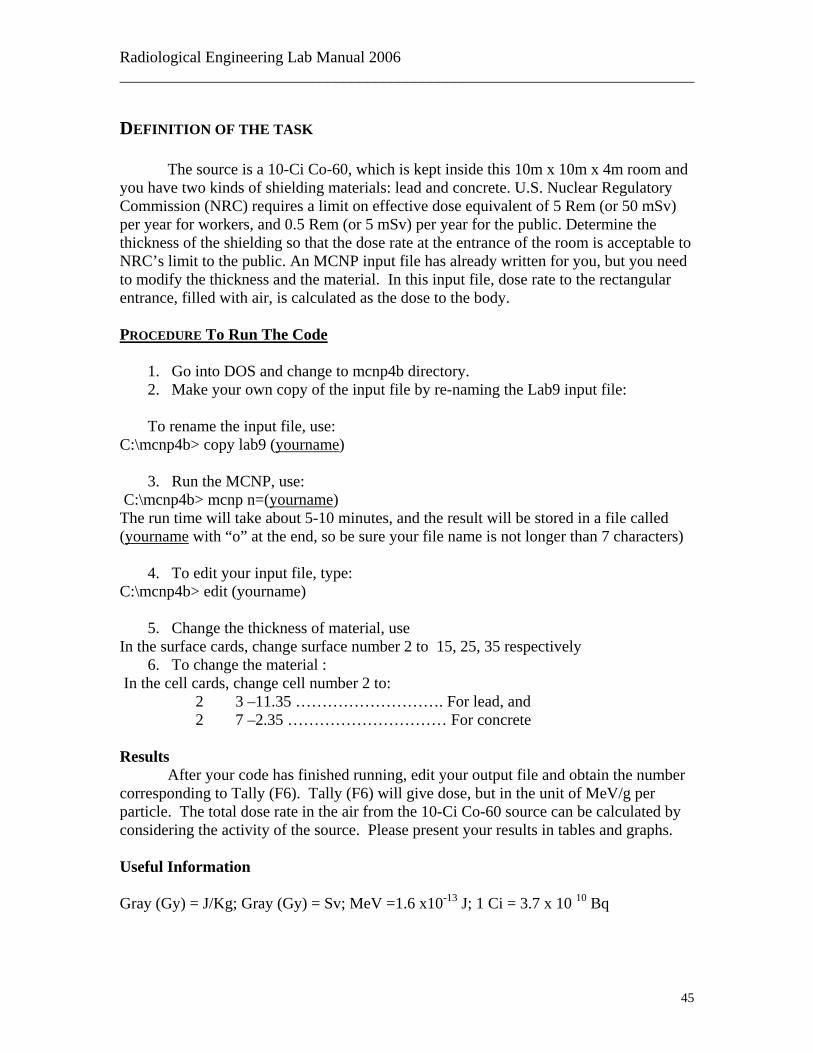
Radiological Engineering Lab Manual 2006 ________________________________________________________________________
DEFINITION OF THE TASK The source is a 10-Ci Co-60, which is kept inside this 10m x 10m x 4m room and you have two kinds of shielding materials: lead and concrete. U.S. Nuclear Regulatory Commission (NRC) requires a limit on effective dose equivalent of 5 Rem (or 50 mSv) per year for workers, and 0.5 Rem (or 5 mSv) per year for the public. Determine the thickness of the shielding so that the dose rate at the entrance of the room is acceptable to NRC’s limit to the public. An MCNP input file has already written for you, but you need to modify the thickness and the material. In this input file, dose rate to the rectangular entrance, filled with air, is calculated as the dose to the body. PROCEDURE To Run The Code
1. Go into DOS and change to mcnp4b directory. 2. Make your own copy of the input file by re-naming the Lab9 input file: To rename the input file, use:
C:\mcnp4b> copy lab9 (yourname)
3. Run the MCNP, use: C:\mcnp4b> mcnp n=(yourname) The run time will take about 5-10 minutes, and the result will be stored in a file called (yourname with “o” at the end, so be sure your file name is not longer than 7 characters)
4. To edit your input file, type: C:\mcnp4b> edit (yourname)
5. Change the thickness of material, use In the surface cards, change surface number 2 to 15, 25, 35 respectively
6. To change the material : In the cell cards, change cell number 2 to:
2 3 –11.35 ………………………. For lead, and 2 7 –2.35 ………………………… For concrete
Results After your code has finished running, edit your output file and obtain the number corresponding to Tally (F6). Tally (F6) will give dose, but in the unit of MeV/g per particle. The total dose rate in the air from the 10-Ci Co-60 source can be calculated by considering the activity of the source. Please present your results in tables and graphs. Useful Information Gray (Gy) = J/Kg; Gray (Gy) = Sv; MeV =1.6 x10⁻¹³ J; 1 Ci = 3.7 x 10 10 Bq
45
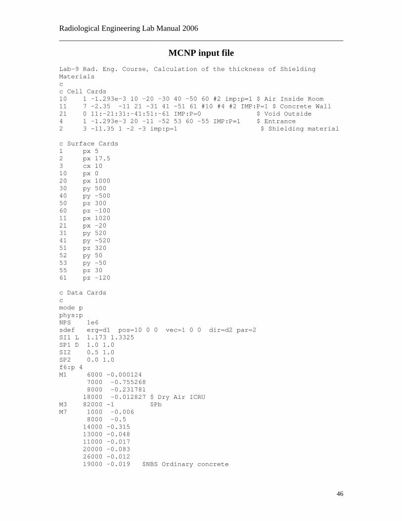
Radiological Engineering Lab Manual 2006 ________________________________________________________________________
MCNP input file Lab-9 Rad. Eng. Course, Calculation of the thickness of Shielding Materials c c Cell Cards 10 1 -1.293e-3 10 -20 -30 40 -50 60 #2 imp:p=1 $ Air Inside Room 11 7 -2.35 -11 21 -31 41 -51 61 #10 #4 #2 IMP:P=1 $ Concrete Wall 21 0 11:-21:31:-41:51:-61 IMP:P=0 $ Void Outside 4 1 -1.293e-3 20 -11 -52 53 60 -55 IMP:P=1 $ Entrance 2 3 -11.35 1 -2 -3 imp:p=1 $ Shielding material c Surface Cards 1 px 5 2 px 17.5 3 cx 10 10 px 0 20 px 1000 30 py 500 40 py -500 50 pz 300 60 pz -100 11 px 1020 21 px -20 31 py 520 41 py -520 51 pz 320 52 py 50 53 py -50 55 pz 30 61 pz -120 c Data Cards c mode p phys:p NPS 1e6 sdef erg=d1 pos=10 0 0 vec=1 0 0 dir=d2 par=2 SI1 L 1.173 1.3325 SP1 D 1.0 1.0 SI2 0.5 1.0 SP2 0.0 1.0 f6:p 4 M1 6000 -0.000124 7000 -0.755268 8000 -0.231781 18000 -0.012827 $ Dry Air ICRU M3 82000 -1 $Pb M7 1000 -0.006 8000 -0.5 14000 -0.315 13000 -0.048 11000 -0.017 20000 -0.083 26000 -0.012 19000 -0.019 $NBS Ordinary concrete
46