The photometric track

Raffaello Sanzio, Lo sposalizio della Vergine, 1504, Milano, Pinacoteca di Brera

Michelangelo, 1528

Lo sposalizio della Vergine Raffaello Sanzio – Pinacoteca di Brera

Standard nearby point source model• N is the surface normal, is diffuse albedo, S is source vector whose

length is the intensity term

Assume that all points in the model are close to each other with respect to the distance to the source. Then the source vector doesn’t vary much, and the distance doesn’t vary much either, the computation are simplified.

2

xr

xSxNxd

NS

Nearby point source model Distant point source model

xSxNx dd

N

S

A photon’s life choices

• Absorption

• Diffusion

• Reflection

• Transparency

• Refraction

• Fluorescence

• Subsurface scattering

• Phosphorescence

• Inter-reflection

λ

light source

?

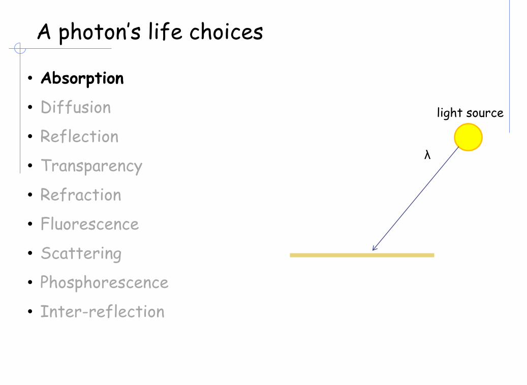
A photon’s life choices

• Absorption

• Diffusion

• Reflection

• Transparency

• Refraction

• Fluorescence

• Scattering

• Phosphorescence

• Inter-reflection

λ

light source

A photon’s life choices

• Absorption

• Diffuse Reflection

• Reflection

• Transparency

• Refraction

• Fluorescence

• Scattering

• Phosphorescence

• Interreflection

λ

light source

A photon’s life choices

• Absorption

• Diffusion

• Specular Reflection

• Transparency

• Refraction

• Fluorescence

• Scattering

• Phosphorescence

• Inter-reflection

λ

light source

A photon’s life choices

• Absorption

• Diffusion

• Reflection

• Transparency

• Refraction

• Fluorescence

• Scattering

• Phosphorescence

• Interreflection

λ

light source

A photon’s life choices

• Absorption

• Diffusion

• Reflection

• Transparency

• Refraction

• Fluorescence

• Scattering

• Phosphorescence

• Interreflection

λ

lightsource

A photon’s life choices

• Absorption

• Diffusion

• Reflection

• Transparency

• Refraction

• Fluorescence

• Scattering

• Phosphorescence

• Interreflection

λ1

light source

λ2

A photon’s life choices

• Absorption

• Diffusion

• Reflection

• Transparency

• Refraction

• Fluorescence

• Subsurface scattering

• Phosphorescence

• Interreflection

λ

light source

A photon’s life choices

• Absorption

• Diffusion

• Reflection

• Transparency

• Refraction

• Fluorescence

• Scattering

• Phosphorescence

• Interreflection

t=1

light source

t=n

A photon’s life choices

• Absorption

• Diffusion

• Reflection

• Transparency

• Refraction

• Fluorescence

• Scattering

• Phosphorescence

• Inter-reflection

λ

light source

(Specular Interreflection)

Local rendering

• Optical geometry of the light-source/eye-receiver system

• Notation:

• n is the normal to the surface at the incidence point

• î corresponds to the incidence angle

• â = î is the reflectance angle

• ô is the mirrored emergence angle

• û is the phase angle

• ê is the emergence angle.

13

n

ôû

â î

ê

The Lambertian model

14

2 2

0

ˆˆcos

elsewhere

n

î

The specular model

15

2 2

0

ˆˆcosm o

elsewhere

o

n

â îô

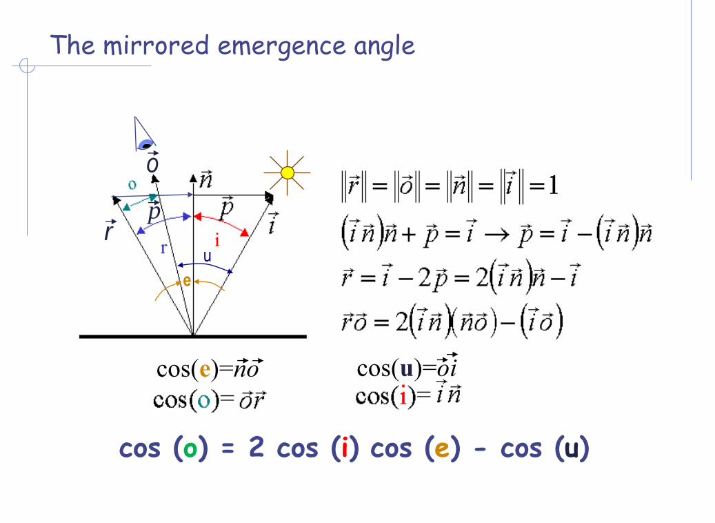
The mirrored emergence angle

cos (o) = 2 cos (i) cos (e) - cos (u)

r

o

e

u

cos(e)=no cos(u)=oi

p

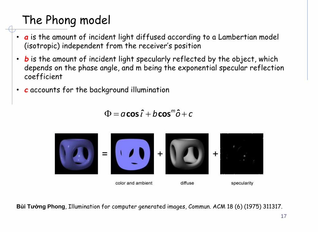
The Phong model

• a is the amount of incident light diffused according to a Lambertian model (isotropic) independent from the receiver’s position

• b is the amount of incident light specularly reflected by the object, which depends on the phase angle, and m being the exponential specular reflection coefficient

• c accounts for the background illumination

Bùi Tường Phong, Illumination for computer generated images, Commun. ACM 18 (6) (1975) 311317.

17

ˆˆcos cosma b o c

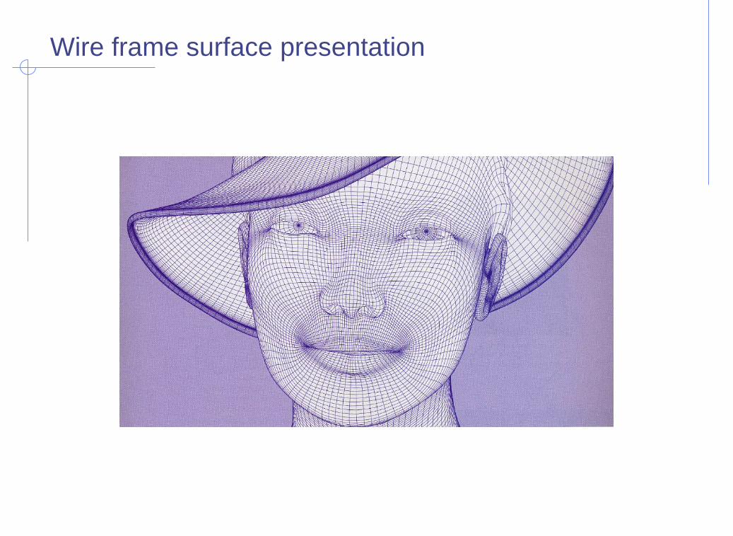
Wire frame surface presentation

Local rendering

http://www.danielrobichaud.com/animation/#/marlene/

Sphere (m=10, c=0)

a=1.0

1.00.0

b=0.0 0.8 0.2 0.6 0.4

0.2 0.8 0.4 0.6

Specular sphere (b=0.9, c=0.1)

m=1

m=1000 m=100 m=10

m=3 m=6

Computing light source directions

• Trick: place a chrome sphere in the scene

the location of the highlight tells you where the light source is

N

rN

C

H

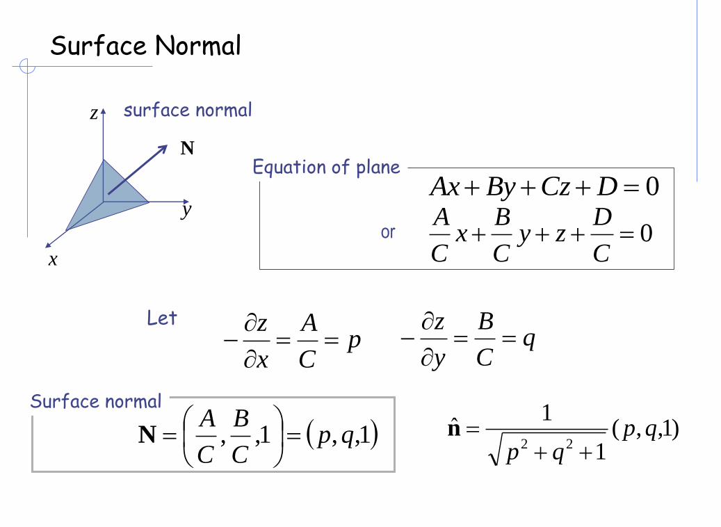
Surface Normal

N

surface normal

y

z

x

0 DCzByAx

0C

Dzy

C

Bx

C

Aor

Letp

C

A

x

z

q

C

B

y

z

1,,1,, qpC

B

C

A

N

Surface normal

Equation of plane

)1,,(1

1ˆ

22qp

qp n

Gradient space

x

fp

y

fq

)1,,(1

1ˆ

)1,,(

22qp

qp

qp

n

n

(p,q,1)z=1

),( yxfz

Gradient Space

y

z

x

1z

q

p

1

s n

N

1

1,,

22

qp

qp

N

Nn

1

1,,

22

SS

SS

qp

qp

S

Ss

Normal vector

Source vector

i

11

1cos

2222

SS

SSi

qpqp

qqppsn

1z plane is called the Gradient Space (p q plane)

Every point on it corresponds to a particular surface orientation

S

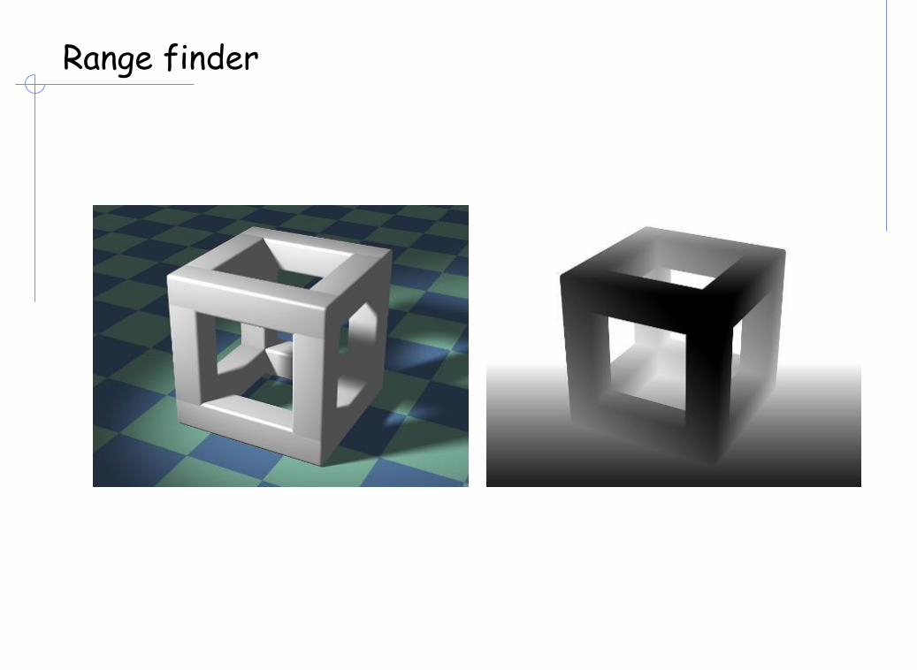
Range finder

Reflectance maps

• Let us take a reference system where the optical axis of the acquisition system (the receiver) coincides with the z axis.

• The surface described by the function z = f(x, y) has the normal vector: (∂z/∂x, ∂z/∂y, -1)t.

• Calling p=∂z/∂x and q=∂z/∂y there is a one-to-onecorrespondence between the plane p, q (called gradientplane) and the normal directions to the surface.

• The three angles î, û and ê may be computed with the following formulas:

27

2 2 2 2

1

1 1ˆcos s s

s s

pp qq

p q p q

2 2

1

1ˆcos e

p q

2 2

1

1ˆcos

s s

up q

Reflectance maps

• reflectivity map for a Lambertian case having both camera and light source coincident with the z-axis (0, 0, -1);

• the specular case having the specularity index m=3;

• an intermediate case with a = b = 0.5, m=3 and c = 0

28

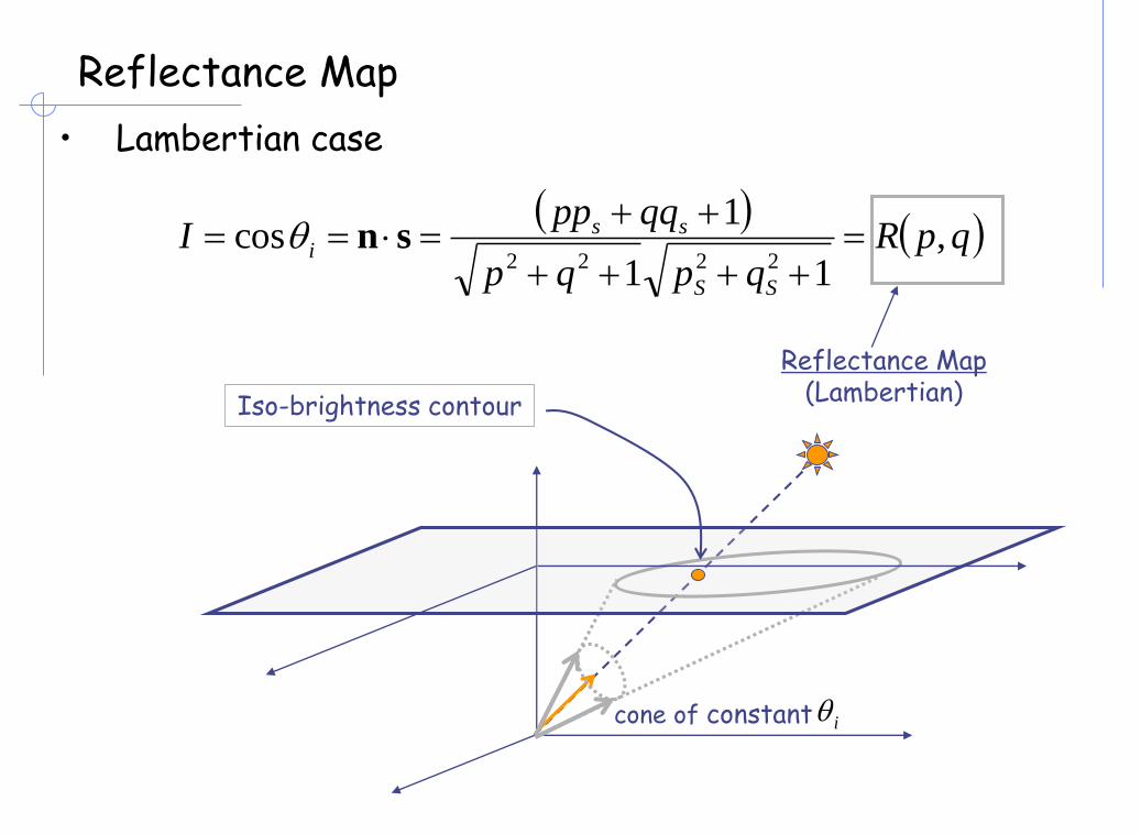
Reflectance Map

• Lambertian case

qpR

qpqp

qqppI

SS

ssi ,

11

1cos

2222

sn

Reflectance Map(Lambertian)

cone of constant i

Iso-brightness contour

Reflectance Map

• Lambertian case

0.1

3.0

0.0

9.08.0

7.0, qpR

p

q

90i 01 SS qqpp

SS qp ,

iso-brightness contour

Note: is maximum when qpR , SS qpqp ,,

Reflectance maps

• Reflectivity map for a Lambertian model; having the camera on the z-axis (0,0,-1) and the light source positioned at (1, 1, -1). The isoluminance patterns are quadrics labelled with their corresponding ratios, the incident light source corresponds to the bisector of the first octant in 3D space.

• Reflectivity map for a specular model having the specularity index is m = 3.

31

Shape from a Single Image?

• Given a single image of an object with known surface reflectance taken under a known light source, can we recover the shape of the object?

• Two reflectance maps?

p

q

bqpR ),(1

aqpR ),(2

Intersections:2 solutions for

p and q.

Photometric Stereo

p

q

11 ,SS

qp

22 ,SS

qp

33 ,SS

qp

Photometric analysis

• Overlapped isoluminance patterns, for the Lambertian model, with threedifferent positions of the light source used [(1,1,-1), (0,0,-1), (-1, 1,-1)] for determining the attitude of an object’s facet.

35

1=0,95

2=0,3

2=0,1

Radiometric Camera Calibration

• Pixel intensities are usually not proportional to the energy that hit the CCD

RAW image Published image

Austin Abrams

f

RAW

Published

Radiometric Camera Calibration

Observed = f(RAW)

(Grossberg and Nayar)f -1 (Observed) = RAW

Vision is Inferential

Prior Knowledge

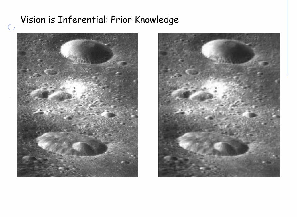
Vision is Inferential: Prior Knowledge

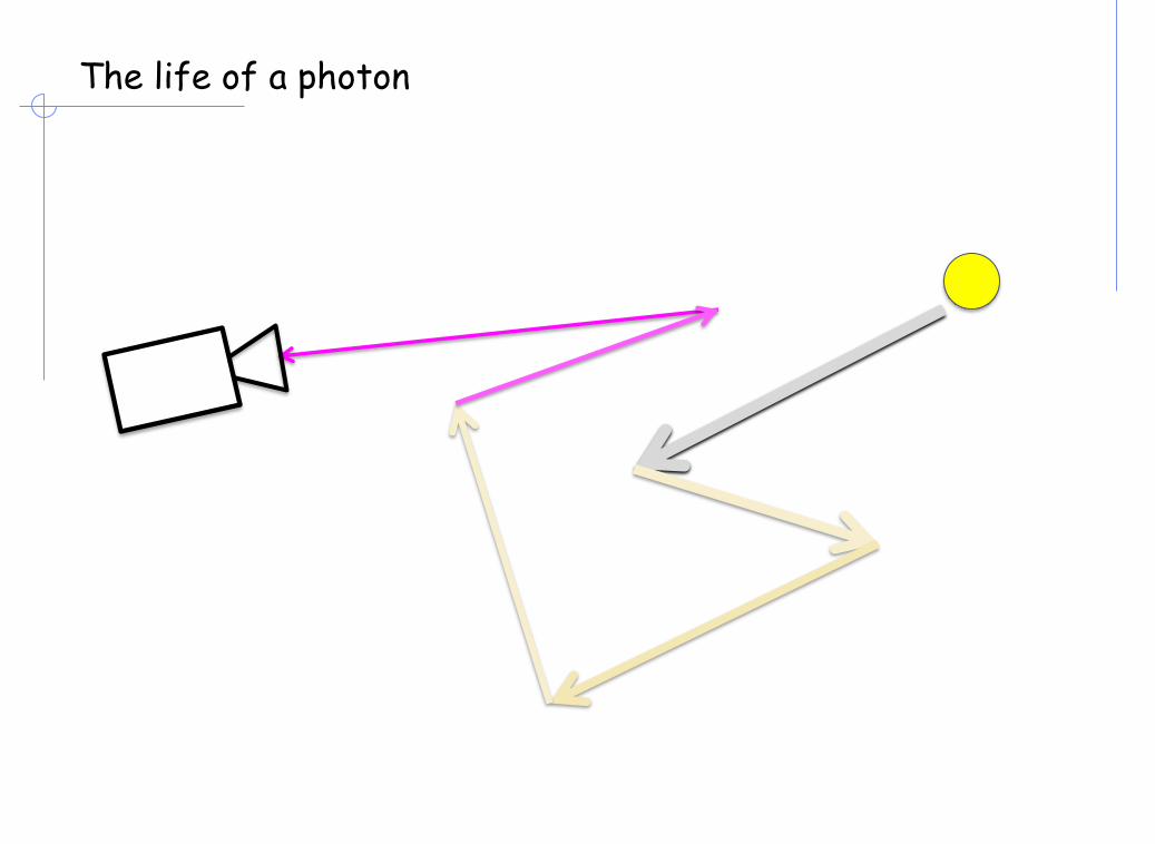
The life of a photon

Global rendering: ray tracing• The two basic schemes of forward (source to eye) and backward (eye

to source) ray tracing, this last is computationally efficient but and cannot properly model diffuse reflections and all other changes in light intensity due to non-specular reflections

41

Image Plane

Light

Image Plane

Light

Global rendering: ray tracing• A ray sent from the eye to the scene

through the image plane may intersect an object; in this case secondary rays are sent out and three different lighting models can be considered:

• transmission. The secondary ray is sent in the direction of refraction, following the Descartes’law;

• reflection. The secondary ray is sent in the direction of reflection, and the Phong model is applied;

• shadowing. The secondary ray is sent toward a light source, if intercepted by an object the point is shadowed.

Figure. A background pixel corresponding to the ray P1 and a pixel representing an object (ray P2). The secondary rays triggered by the primary ray P2 according to the three models: transmission (T1 and T2), reflection (R1, R2

and R3), and tentative shadowing (S1, S2: true shadows, and S3).

42

Image plane

Light

Opaqueobject

Opaqueobject

Opaqueobject

Transparentobject

P1

P2

R1

R2

R3

S1

S3

S2

T1

T2

Reflections and transparencies

Created by David Derman – CISC 440

Example

Global rendering: radiosity• The radiosity method has been developed to model the

diffuse-diffuse interactions so gaining a more realistic visualization of surfaces.

• The diffused surfaces scatter light in all directions (i.e. in Lambertian way). Thus a scene is divided into patches -small flat polygons. For each patch the goal is to measure energies emitted from and reflected to respectively. The radiosity of the patch i is given by:

• Where represents the energy emitted by patch i,

the reflectivity parameter of patch i, and

the energy reflected to patch i from the n patches jaround it, depending on the form factors .

• The form factor represents the fraction of light thatreaches patch i from patch j. It depends on the distanceand orientation of the two patches.

• A scene with n patches, follows a system of n equations for which the solution yields the radiosity of each patch.

45

Ai

Aj

Ni

Nj

r

j

i

dAi

dAj

1

n

i i i j ijj

B E B F

Example

Global illumination photon mapping• Photon mapping is a two-pass algorithm developed by Henrik Wann Jensen that approximately solves

the rendering equation.

• Rays from the light source and rays from the camera are traced independently until some termination criterion is met, then they are connected in a second step to produce a radiance value.

• It is used to realistically simulate the interaction of light with different objects. Specifically, it is capable of simulating the refraction of light through a transparent substance such as glass or water, diffuse interreflection between illuminated objects, the subsurface scattering of light in translucent materials, and some of the effects caused by particulate matter such as smoke or water vapor.

Example

A comparison by Ledah Casburn

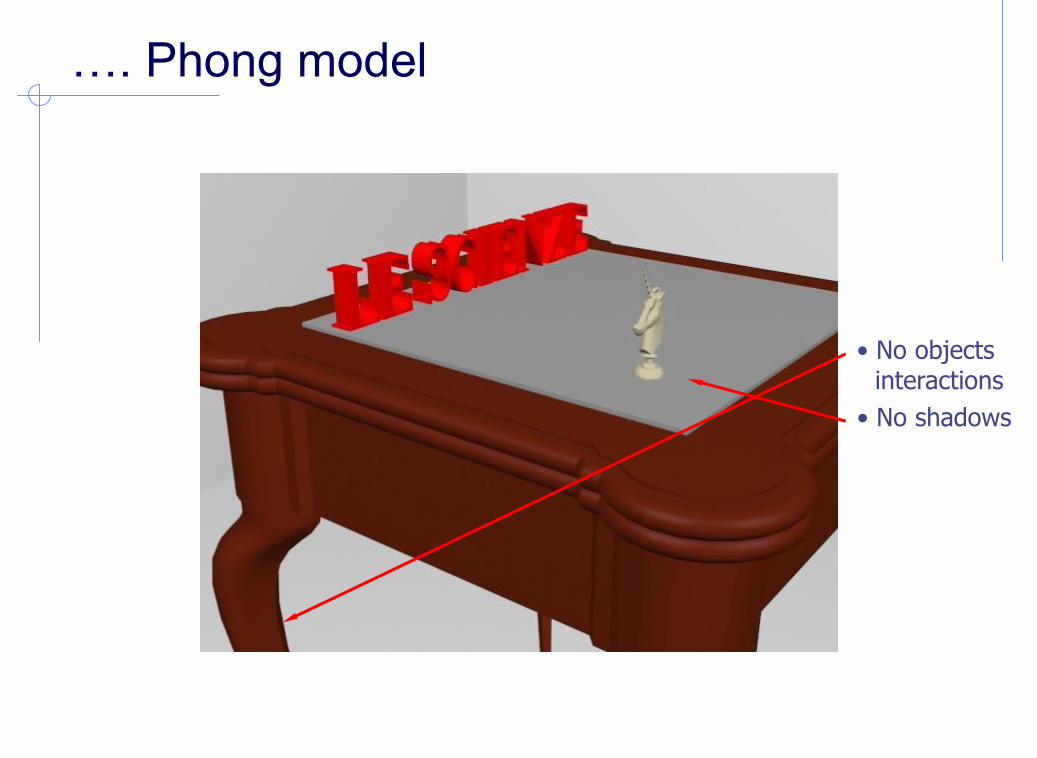
…. Phong model

• No shadows

• No objects interactions

… ray tracing

• is there a corner?

• is the floor properlyrendered?

• is the window in depth?

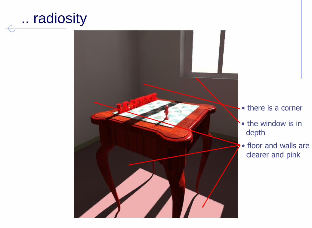
.. radiosity

• floor and walls are clearer and pink

• the window is in depth

• there is a corner

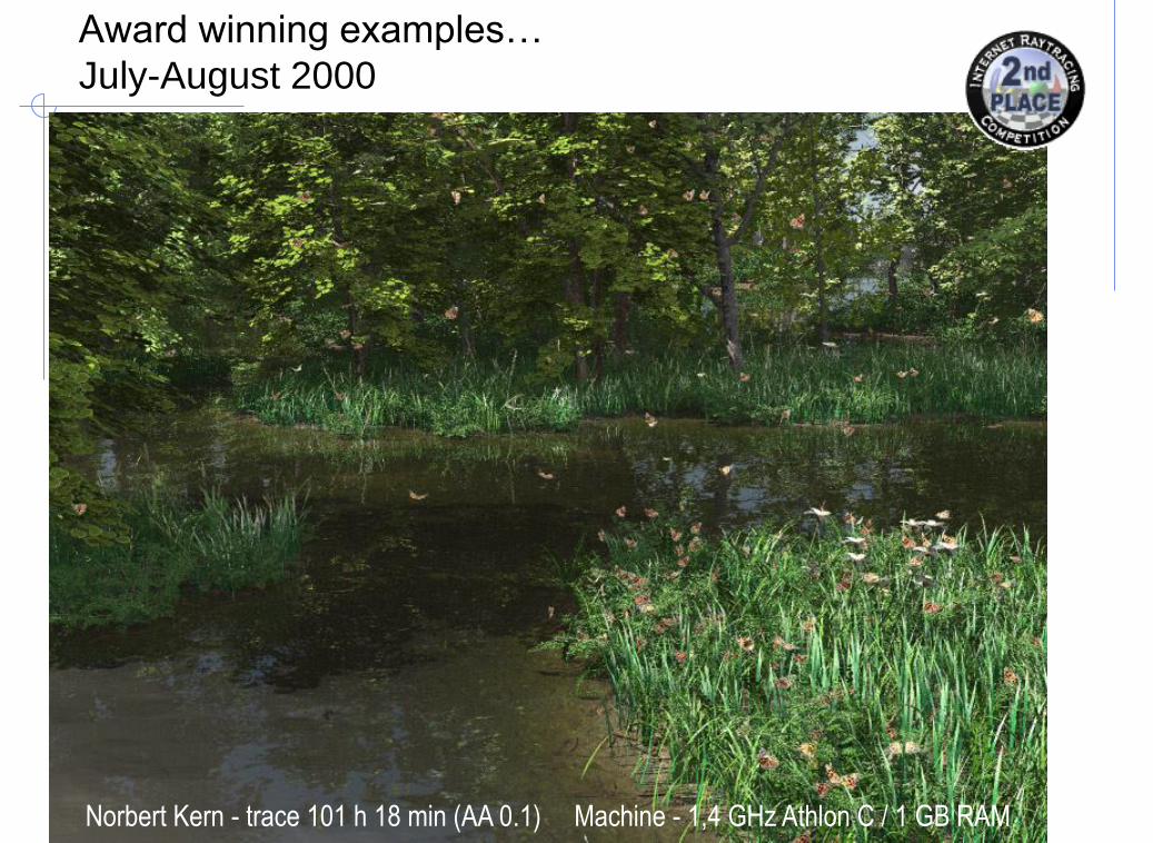
Award winning examples…

July-August 2000

Norbert Kern - trace 101 h 18 min (AA 0.1) Machine - 1,4 GHz Athlon C / 1 GB RAM

Example: Render of the year 2014

The betrothal of the Arnolfini

Jan Van Eyck 1434, National Gallery, London

Examples

Synthesys: basics

• Texture: definitions

Texture—the appearance and feel of a surface

Texture—an image used to define the characteristics of a surface

Texture—a multidimensional image which is mapped to a multidimensional space

Materials and Texture Maps

• Using materials and textures can create attributes such as colour, transparency, and shininess of an object. Materials control how the light interacts with the an object’s surface

• Textures are image that can be ‘mapped’ to geometry to provide authentic surface detail and characteristics.

• Texture maps are useful for providing a look for an object where a high level of detail is not required for an objects geometry - brick walls, guitar fret board for example.

• Texture maps can also be used to replace distant geometry where level of detail is such that it permits the substitution of the geometry with a textured primitive object.

• Texture maps can themselves be combined with to provide layered texturing characteristics to achieve the desired modelling effect

Texture mapping

• Texture mapping maps image onto surface, two approaches:

Forward Mapping- Each points in the image is mapped onto the polygon

- Harder to implement correctly, and harder to model

Inverse Mapping- Each vertex is associated with a point on an image (u,v)

- Inverse mapping is much more commonly used

- Most 3D modelers output U,V co-ordinates for texture application

• Texture types: http://wiki.polycount.com/wiki/Texture_types

Basic Concept

• “Slap an image on a model”, better: “A mapping from any function onto a surface in 3D”, most general: “The mapping of any image into multi-dimensional space.”

• How do we map a two-dimensional image to a surface in three dimensions?

• Texture coordinates

2D coordinate (u,v) which maps to a location on the image

Assign a texture coordinate to each vertex

Coordinates are determined by some function which maps a texture location to a vertex on the model in three dimensions

• Once a point on the surface of the model has been mapped to a value in the texture, change its RGB value (or something else!) accordingly

• This is called parametric texture mapping• A single point in the texture is called a

texel

Texture mapping, an objective:

+ =

3D mesh 2D texture (color-map)

+ =

Texture mapping

• UV Mapping is the process of mapping a 2D coordinate grid to a 3D model The 2D grid is associated with a corresponding image file to place on the model. UV coordinates (also known as texture coordinates) can be generated for each vertex in the mesh. One way is to unfold the mesh at the seams, automatically laying out on a flat page.

• Once the model is unwrapped the scene may be rendered combining each mesh element to the appropriate texture image

Unwrappingexample of

cube

Unwrappingexample of

head

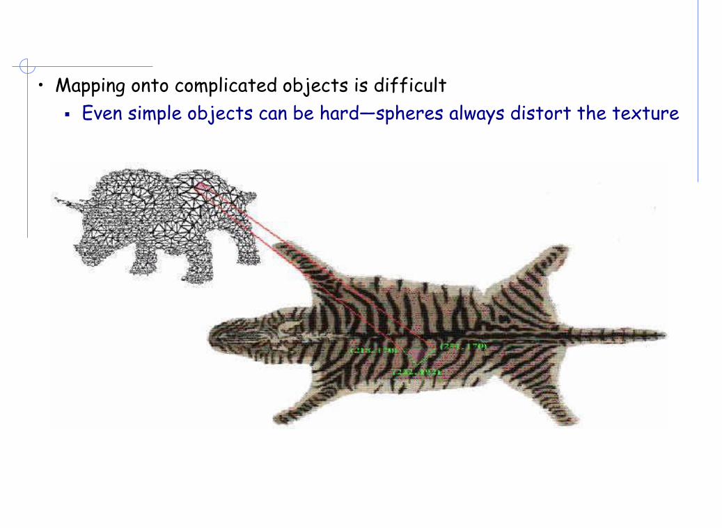
• Mapping onto complicated objects is difficult

Even simple objects can be hard—spheres always distort the texture

Color and Ambient Occlusion maps

• Texture maps are developed to directly correspond to the UV coordinates of an unwrapped

3D model:

• Color map: As the name would imply, the most obvious use for a texture map is to add color or texture to the surface of a model. However, surface maps play a huge role in computer graphics beyond just color and texture. In a production setting, a character or environment's color map is usually just one of the maps that will be used for almost every single 3D model.

• AO (Ambient Occlusion) map: are pre-computed calculations of ambient light bounce on a surface, keeping dark shadows to crevices and sharp corners only. It is used with the color map, combining color information in multiplication. It is in gray gradations, often with strong contrast. The purpose is to darken the color map hues to create shadows, increasing the 3D effect without weighing the calculation. The objective is to simulate the environmental illumination in areas enclosed on the surface.

Color mapexample of

bricks

AO mapexample of

bricks

Specular and Roughness maps• Specular map (or shininess or gloss map): A specular map tells the software which parts of a

model should be shiny or glossy, and also the magnitude of the glossiness. Specular maps are named for the fact that shiny surfaces, like metals, ceramics, and some plastics show a strong specular highlight (a direct reflection from a strong light source). White areas correspond to the highest shininess meanwhile black areas to the null case.

• Roughness/Reflective map: tells the software which portions of the 3D model should be

lambertian. If a model's entire surface is reflective, or if the level of reflectivity is uniform a

reflection map is usually omitted. Reflection maps are grayscale images, with black indicating 0%

(100%) reflectivity and pure white indicating a 100% (0%) reflective surface.

Specular mapexample of

bricks

Roughness mapexample of

bricks(lack of

specularity)

Normal and Height maps• Normal map (o bump-map): normal maps are a type of texture map that can help give a more

realistic indication of bumps or depressions on the surface of a model. Consider a brick wall: to increase the impression of realism, a bump or normal map would be added to more accurately recreate the coarse, grainy surface of bricks, and heighten the illusion that the cracks between bricks are actually receding in space.

• Height map: are typically used to deform terrain meshes moving vertices up and down. Displacement maps are similar to bump but store height information and modify geometry when rendered, modifying both appearance of shading and silhouette. The rendering of the normal map is limited when the viewer is close to the object and looks at it from a low angle. In such cases, other maps are used, such as displacement map or heigh tmap, physically sculpting the details on the surface, obviously increasing the polygonal density. The point data (intensity) is interpreted by the 3D editor as the distance of vertices from a base quota defined as 0

Esempio di Normal mapdi mattoni

Esempio di Height mapdi mattoni

Environment Mapping

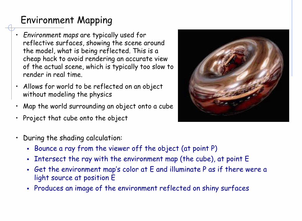
• Environment maps are typically used for reflective surfaces, showing the scene around the model, what is being reflected. This is a cheap hack to avoid rendering an accurate view of the actual scene, which is typically too slow to render in real time.

• Allows for world to be reflected on an object without modeling the physics

• Map the world surrounding an object onto a cube

• Project that cube onto the object

• During the shading calculation:

Bounce a ray from the viewer off the object (at point P)

Intersect the ray with the environment map (the cube), at point E

Get the environment map’s color at E and illuminate P as if there were a light source at position E

Produces an image of the environment reflected on shiny surfaces

Light Mapping

• Texture maps are used to add detail to surfaces, and light maps are used to store pre-computed illumination. The two are multiplied together at run-time, and cached for efficiency.

Radiance Texture Map Only Radiance Texture + Light Map

Light Map

Seamless problem

• The term seamless describes a texture that does not have defined borders once it is duplicated and flanked to itself: the result is a homogeneous pattern on which one can not distinguish a textel from the other. Often a photo retouching step is needed. In many cases the images provided by on-line texture libraries are already seamless, otherwise you can remedy them with the various tools available. Then you work on color correction and reduce direct lighting and in some cases also eliminate defects in texture, such as spots or breaks that become recursive.