random design analysis of ridge regressiondjhsu/papers/ridge-colt.pdfrandom design analysis of ridge...

JMLR: Workshop and Conference Proceedings vol:1–24, 2012 25th Annual Conference on Learning Theory

Random Design Analysis of Ridge Regression

Daniel Hsu [email protected] Research

Sham M. Kakade [email protected] Research

Tong Zhang [email protected]

Rutgers University

Editor: Shie Mannor, Nathan Srebro, Bob Williamson

Abstract

This work gives a simultaneous analysis of both the ordinary least squares estimator andthe ridge regression estimator in the random design setting under mild assumptions on thecovariate/response distributions. In particular, the analysis provides sharp results on the“out-of-sample” prediction error, as opposed to the “in-sample” (fixed design) error. Theanalysis also reveals the effect of errors in the estimated covariance structure, as well asthe effect of modeling errors; neither of which effects are present in the fixed design setting.The proof of the main results are based on a simple decomposition lemma combined withconcentration inequalities for random vectors and matrices.

1. Introduction

In the random design setting for linear regression, we are provided with samples of covari-ates and responses, (x1, y1), (x2, y2), . . . , (xn, yn), which are sampled independently from apopulation, where the xi are random vectors and the yi are random variables. Typically,these pairs are hypothesized to have the linear relationship

yi = 〈β, xi〉+ εi

for some linear function β (though this hypothesis need not be true). Here, the εi are errorterms, typically assumed to be normally distributed as N (0, σ2). The goal of estimationin this setting is to find coefficients β based on these (xi, yi) pairs such that the expectedprediction error on a new draw (x, y) from the population, measured as E[(〈β, x〉 − y)2],is as small as possible. This goal can also be interpreted as estimating β with accuracymeasured under a particular norm.

The random design setting stands in contrast to the fixed design setting, where thecovariates x1, x2, . . . , xn are fixed (i.e., deterministic), and only the responses y1, y2, . . . , yntreated as random. Thus, the covariance structure of the design points is completely knownand need not be estimated, which simplifies the analysis of standard estimators. However,the fixed design setting does not directly address out-of-sample prediction, which is ofprimary concern in many applications. For instance, in prediction problems, the estimatorβ is computed from an initial sample from the population, and the end-goal is to use β asa predictor of y given x where (x, y) is a new draw from the population. A fixed design

c© 2012 D. Hsu, S.M. Kakade & T. Zhang.

Hsu Kakade Zhang

analysis only assesses the accuracy of β on data already seen, while a random design analysisis concerned with the predictive performance on unseen data.

This work gives a detailed analysis of both the ordinary least squares and ridge esti-mator (Hoerl, 1962) in the random design setting that quantifies the essential differencesbetween random and fixed design. In particular, the analysis reveals, through a simple de-composition, the effect of errors in the estimated covariance structure, as well as the effectof approximating the true regression function by a linear function in the case the model ismisspecified. Neither of these effects is present in the fixed design analysis of ridge regres-sion. The random design analysis shows that the effect of errors in the estimated covariancestructure is minimal—it is typically a second-order effect as soon as the sample size is largeenough. The analysis also isolates the effect of approximation error in the main terms of theestimation error bound so that the bound reduces to one that scales with the noise variancewhen the approximation error vanishes.

One feature of the analysis in this work is that it applies to the ridge estimator withan arbitrary setting of λ. The estimation error is given in terms of the spectrum of thecovariance E[x ⊗ x] and the particular choice of λ. When λ = 0, we obtain an analysis ofordinary least squares, applicable when the spectrum is finite (i.e., when the covariates livein a finite dimensional space). More generally, the convergence rate can be optimized byappropriately setting λ based on assumptions about the spectrum.

Outline. Section 2 discusses the model, preliminaries, and related work. Section 3 presentsthe main results on the excess mean squared error of the ordinary least squares and ridgeestimators under random design and discusses the relationship to the standard fixed designanalysis. An application to smoothing splines is provided in Appendix A, and the proof ofthe main results are given in the Appendix B.

2. Preliminaries

2.1. Notation

Unless otherwise specified, all vectors in this work are assumed to live in a (possiblyinfinite dimensional) separable Hilbert space with inner product 〈·, ·〉. Let ‖ · ‖M for aself-adjoint positive semidefinite linear operator M � 0 denote the vector norm given by‖v‖M :=

√〈v,Mv〉. When M is omitted, it is assumed to be the identity, so ‖v‖ =

√〈v, v〉.

Let u⊗u denote the outer product of a vector u, which acts as the rank-one linear operatorv 7→ (u ⊗ u)v = 〈v, u〉u. For a linear operator M , let ‖M‖ denote its spectral (opera-tor) norm, i.e., ‖M‖ = supv 6=0 ‖Mv‖/‖v‖, and let ‖M‖F denote its Frobenius norm, i.e.,

‖M‖F =√

tr(M∗M). If M is self-adjoint, ‖M‖F =√

tr(M2). Let λmax[M ] and λmin[M ],respectively, denote the largest and smallest eigenvalue of a self-adjoint linear operator M .

2.2. Linear regression

Let x be a random vector, and let y be a random variable. Let {vj} be the eigenvectors of

Σ := E[x⊗ x], (1)

so that they form an orthonormal basis. The corresponding eigenvalues are

λj := 〈vj , Σvj〉 = E[〈vj , x〉2]

2


(assumed to be non-zero for convenience). Let β achieve the minimum mean squared errorover all linear functions, i.e.,

E[(〈β, x〉 − y)2] = minw

{E[(〈w, x〉 − y)2]

},

so that:

β :=∑j

βjvj where βj :=E[〈vj , x〉y]

E[〈vj , x〉2]. (2)

We also have that the excess mean squared error of w over the minimum is:

E[(〈w, x〉 − y)2]− E[(〈β, x〉 − y)2] = ‖w − β‖2Σ

(see Proposition 21).

2.3. The ridge and ordinary least squares estimators

Let (x1, y1), (x2, y2), . . . , (xn, yn) be independent copies of (x, y), and let E denote the em-pirical expectation with respect to these n copies, i.e.,

E[f ] :=1

n

n∑i=1

f(xi, yi) Σ := E[x⊗ x] =1

n

n∑i=1

xi ⊗ xi. (3)

Let βλ denote the ridge estimator with parameter λ ≥ 0, defined as the minimizer ofthe λ-regularized empirical mean squared error, i.e.,

βλ := arg minw

{E[(〈w, x〉 − y)2] + λ‖w‖2

}. (4)

The special case with λ = 0 is the ordinary least squares estimator, which minimizes theempirical mean squared error. These estimators are uniquely defined if and only if Σ+λI �0 (a sufficient condition is λ > 0), in which case

βλ = (Σ + λI)−1E[xy].

2.4. Data model

We now specify the conditions on the random pair (x, y) under which the analysis applies.

2.4.1. Covariate model

The following conditions on the covariate x ensure that the second-moment operator Σ canbe estimated from a random sample with sufficient accuracy. The first requires that thespectrum of Σ decays sufficiently fast at regularization level λ.

Condition 1 (Spectral decay at λ) For p ∈ {1, 2},

dp,λ :=∑j

(λj

λj + λ

)p<∞. (5)

3

Hsu Kakade Zhang

For technical reasons, we also use the quantity

d1,λ := max{d1,λ, 1} (6)

merely to simplify certain probability tail inequalities in the main result in the peculiar casethat λ → ∞ (upon which d1,λ → 0). We remark that d2,λ appears naturally arises in thestandard fixed design analysis of ridge regression (see Proposition 5), and that d1,λ was alsoused by Zhang (2005) in his random design analysis of (kernel) ridge regression. It is easyto see that d2,λ ≤ d1,λ, and that in in covariate spaces of finite dimension d < ∞, we havedp,λ ≤ d with equality iff λ = 0.

The second condition requires that the squared length of (Σ + λI)−1/2x is never morethan a constant factor greater than its expectation (hence the name bounded statisticalleverage). The linear mapping x 7→ (Σ + λI)−1/2x is sometimes called whitening whenλ = 0. The reason for considering λ > 0, in which case we call the mapping λ-whitening, isthat the expectation E[‖(Σ + λI)−1/2x‖2] may only be small for sufficiently large λ (as inCondition 1), as

E[‖(Σ + λI)−1/2x‖2] = tr((Σ + λI)−1/2Σ(Σ + λI)−1/2) =∑j

λjλj + λ

= d1,λ.

Condition 2 (Bounded statistical leverage at λ) There exists finite ρλ ≥ 1 such that,almost surely,

‖(Σ + λI)−1/2x‖√E[‖(Σ + λI)−1/2x‖2]

=‖(Σ + λI)−1/2x‖√

d1,λ≤ ρλ.

The hard “almost sure” bound in Condition 2 may be relaxed to moment conditions simplyby using different probability tail inequalities in the analysis. We do not consider thisrelaxation for sake of simplicity. We also remark that, in finite dimensional settings, it iseasy to replace Condition 2 with a subgaussian condition (specifically, a requirement thatevery projection of (Σ + λI)−1/2x be subgaussian), which can lead to a sharper deviationbound in certain cases.

Remark 1 (Finite dimensional setting and λ = 0) If λ = 0 and the dimension of thecovariate space is d, then Condition 2 reduces to the requirement that there exists a finiteρ0 ≥ 1 such that, almost surely,

‖Σ−1/2x‖√E[‖Σ−1/2x‖2]

=‖Σ−1/2x‖√

d≤ ρ0.

Remark 2 (Bounded ‖x‖) If ‖x‖ ≤ r almost surely, then

‖(Σ + λI)−1/2x‖√d1,λ

≤ r√(inf{λj}+ λ)d1,λ

in which case Condition 2 is satisfied with

ρλ ≤r√λd1,λ

.

4


2.4.2. Response model

The response model considered in this work is a relaxation of the typical Gaussian model;the model specifically allows for approximation error and general subgaussian noise. Definethe random variables

noise(x) := y − E[y|x] and approx(x) := E[y|x]− 〈β, x〉 (7)

where noise(x) corresponds to the response noise, and approx(x) corresponds to the ap-proximation error of β. This gives the following modeling equation:

y = 〈β, x〉+ approx(x) + noise(x).

Conditioned on x, noise(x) is random, while approx(x) is deterministic.The noise is assumed to satisfy the following subgaussian moment condition.

Condition 3 (Subgaussian noise) There exists finite σ ≥ 0 such that, almost surely,

E [exp(η noise(x))|x] ≤ exp(η2σ2/2) ∀η ∈ R.

Condition 3 is satisfied, for instance, if noise(x) is normally distributed with mean zero andvariance σ2.

For the next condition, define βλ to be the minimizer of the regularized mean squarederror, i.e.,

βλ := arg minw

{E[(〈w, x〉 − y)2] + λ‖w‖2

}= (Σ + λI)−1E[xy], (8)

and also defineapproxλ(x) := E[y|x]− 〈βλ, x〉. (9)

The final condition requires a bound on the size of approxλ(x).

Condition 4 (Bounded approximation error at λ) There exist finite bλ ≥ 0 such that,almost surely,

‖(Σ + λI)−1/2x approxλ(x)‖√E[‖(Σ + λI)−1/2x‖2]

=‖(Σ + λI)−1/2x approxλ(x)‖√

d1,λ≤ bλ.

The hard “almost sure” bound in Condition 4 can easily be relaxed to moment conditions,but we do not consider it here for sake of simplicity. We also remark that bλ only appearsin lower-order terms in the main bounds.

Remark 3 (Finite dimensional setting and λ = 0) If λ = 0 and the dimension of thecovariate space is d, then Condition 4 reduces to the requirement that there exists a finiteb0 ≥ 0 such that, almost surely,

‖Σ−1/2x approx(x)‖√E[‖Σ−1/2x‖2]

=‖Σ−1/2x approx(x)‖√

d≤ b0.

5

Hsu Kakade Zhang

Remark 4 (Bounded | approx(x)|) If | approx(x)| ≤ a almost surely and Condition 2(with parameter ρλ) holds, then

‖(Σ + λI)−1/2x approxλ(x)‖√d1,λ

≤ ρλ| approxλ(x)|

≤ ρλ(a+ |〈β − βλ, x〉|)≤ ρλ(a+ ‖β − βλ‖Σ+λI‖x‖(Σ+λI)−1)

≤ ρλ(a+ ρλ√d1,λ‖β − βλ‖Σ+λI)

where the first and last inequalities use Condition 2, the second inequality uses the defini-tion of approxλ(x) in (9) and the triangle inequality, and the third inequality follows fromCauchy-Schwarz. The quantity ‖β−βλ‖Σ+λI can be bounded by

√λ‖β‖ using the arguments

in the proof of Proposition 23. In this case, Condition 4 is satisfied with

bλ ≤ ρλ(a+ ρλ√λd1,λ‖β‖).

If in addition ‖x‖ ≤ r almost surely, then Condition 2 and Condition 4 are satisfied with

ρλ ≤r√λd1,λ

and bλ ≤ ρλ(a+ r‖β‖)

as per Remark 2.

2.5. Related work

Many classical analyses of the ridge and ordinary least squares estimators in the randomdesign setting (e.g., in the context of non-parametric estimators) do not actually shownon-asymptotic O(d/n) convergence of the mean squared error to that of the best linearpredictor, where d is the dimension of the covariate space. Rather, the error relative to theBayes error is bounded by some multiple c > 1 of the error of the optimal linear predictorrelative to Bayes error, plus a O(d/n) term (Gyorfi et al., 2004):

E[(〈β, x〉 − E[y|x])2] ≤ c · E[(〈β, x〉 − E[y|x])2] +O(d/n).

Such bounds are appropriate in non-parametric settings where the error of the optimal linearpredictor also approaches the Bayes error at an O(d/n) rate. Beyond these classical results,analyses of ordinary least squares often come with non-standard restrictions on applicabilityor additional dependencies on the spectrum of the second moment matrix (see the recentwork of Audibert and Catoni (2010b) for a comprehensive survey of these results). Forinstance, a result of Catoni (2004, Proposition 5.9.1) gives a bound on the excess meansquared error of the form

‖β − β‖2Σ ≤ O

(d+ log(det(Σ)/det(Σ))

n

),

but the bound is only shown to hold when every linear predictor with low empirical meansquared error satisfies certain boundedness conditions.

6


This work provides ridge regression bounds explicitly in terms of the vector β (as a se-quence) and in terms of the eigenspectrum of the of the second moment matrix Σ. Previousanalyses of ridge regression make strong boundedness assumptions, or fail to give a boundin the case λ = 0 (e.g., Zhang, 2005; Smale and Zhou, 2007; Caponnetto and Vito, 2007;Steinwart et al., 2009). For instance, Zhang assumes ‖x‖ ≤ bx and |〈β, x〉 − y| ≤ bapprox

almost surely, and gives the bound ‖βλ − β‖2Σ ≤ λ‖βλ − β‖2 + c · d1,λ·(bapprox+bx‖βλ−β‖)2

nwhere d1,λ is a notion of effective dimension at scale λ (same as that in Condition 1). The

quantity ‖βλ − β‖ is then bounded by assuming ‖β‖ < ∞. Smale and Zhou assumes themore stringent conditions that |y| ≤ by and ‖x‖ ≤ bx almost surely, and proves the bound

‖βλ − βλ‖2Σ ≤ c · b2xb

2y

λ2n(note that the bound becomes trivial when λ = 0); this is then used

to bound ‖βλ − β‖2Σ under explicit boundedness assumptions on β. Caponnetto and Vitocrucially require boundedness of |β‖ and λ > 0 in their analysis (in particular, in theirTheorem 4), and also have a worse tail behavior with a bound of the form d1,λt

2/n withprobability ≥ 1 − e−t. Finally, Steinwart et al. explicitly require |y| ≤ by and their bounddepends on by in the dominant term; moreover, their bounds require explicit decay condi-tions on the eigenspectrum (Equation 6) and also trivial when λ = 0. Our result for ridgeregression is given explicitly in terms of ‖βλ − β‖2Σ (and therefore explicitly in terms of βas a sequence, the eigenspectrum of Σ, and λ); this quantity vanishes when λ = 0 and canbe bounded even when ‖β‖ is unbounded. We note that ‖βλ − β‖2Σ is precisely the biasterm from the standard fixed design analysis of ridge regression, and therefore is natural toexpect in a random design analysis.

Recently, Audibert and Catoni (2010a,b) derived sharp risk bounds for the ordinary leastsquares and ridge estimators (in addition to specially developed PAC-Bayesian estimators)in a random design setting under very mild assumptions. Their bounds are proved usingPAC-Bayesian techniques, which allows them to achieve exponential tail inequalities underremarkably minimal moment conditions. Their non-asymptotic bound for ordinary leastsquares holds with probability at least 1 − e−t but only for t ≤ lnn. Our result requiresstronger assumptions in some respects, but it avoids this restriction on the probability tailparameter t, and the analysis is arguably more transparent and yields more reasonablequantitative bounds. The analysis of Audibert and Catoni (2010a) for the ridge estimatoris established only in an asymptotic sense and bounds the excess regularized mean squarederror rather than the excess mean squared error itself. Therefore, the results are not directlycomparable to those provided here. It should also be mentioned that a number of otherlinear estimators have been considered in the literature with non-asymptotic predictionerror bounds (e.g., Koltchinskii, 2006; Audibert and Catoni, 2010a,b), but the focus of ourwork is on the ordinary least squares and ridge estimators.

3. Random Design Regression

This section presents the main results of the paper on the excess mean squared error of theridge estimator under random design (and its specialization to the ordinary least squaresestimator). First, we review the standard fixed design analysis.

7

Hsu Kakade Zhang

3.1. Review of fixed design analysis

It is informative to first review the fixed design analysis of the ridge estimator. Recallthat in this setting, the design points x1, x2, . . . , xn are fixed (deterministic) vectors, andthe responses y1, y2, . . . , yn are independent random variables. Therefore, we define Σ :=Σ = n−1

∑ni=1 xi ⊗ xi (which is non-random), and assume it has eigenvectors {vj} and

corresponding eigenvalues λj := 〈vj , Σvj〉. As in the random design setting, the linearfunction β :=

∑j βjvj where βj := (nλj)

−1∑ni=1〈vj , xi〉E[yi] minimizes the expected mean

squared error, i.e.,

β := arg minw

1

n

n∑i=1

E[(〈w, xi〉 − yi)2].

Similar to the random design setup, define noise(xi) := yi−E[yi] and approx(xi) := E[yi]−〈β, xi〉 for i = 1, 2, . . . , n, so the following modeling equations holds:

yi = 〈β, xi〉+ approx(xi) + noise(xi)

for i = 1, 2, . . . , n. Because Σ = Σ, the ridge estimator βλ in the fixed design setting is anunbiased estimator of the minimizer of the regularized mean squared error, i.e.,

E[βλ] = (Σ + λI)−1

(1

n

n∑i=1

xiE[yi]

)= arg min

w

{1

n

n∑i=1

E[(〈w, xi〉 − yi)2] + λ‖w‖2}.

This unbiasedness implies that the expected mean squared error of βλ has the bias-variancedecomposition

E[‖βλ − β‖2Σ ] = ‖E[βλ]− β‖2Σ + E[‖βλ − E[βλ]‖2Σ ]. (10)

The following bound on the expected excess mean squared error easily follows from thisdecomposition and the definition of β (see, e.g., Proposition 23).

Proposition 5 (Ridge regression: fixed design) Fix λ ≥ 0, and assume Σ + λI isinvertible. If there exists σ ≥ 0 such that var(y2i ) ≤ σ2 for all i = 1, 2, . . . , n, then

E[‖βλ − β‖2Σ ] ≤∑j

λj

(λjλ + 1)2

β2j +σ2

n

∑j

(λj

λj + λ

)2

with equality iff var(yi) = σ2 for all i = 1, 2, . . . , n.

Remark 6 (Effect of approximation error in fixed design) Observe that approx(xi)has no effect on the expected excess mean squared error.

Remark 7 (Effective dimension) The second sum in the bound is equal to d2,λ fromCondition 1, which implies a notion of effective dimension at regularization level λ.

Remark 8 (Ordinary least squares in fixed design) In finite dimensional spaces ofdimension d, Σ has only d non-zero eigenvalues λj, and therefore setting λ = 0 gives the

following bound for the ordinary least squares estimator β0:

E[‖β0 − β‖2Σ ] ≤ σ2d

n

where, as before, equality holds iff var(yi) = σ2 for all i = 1, 2, . . . , n.

8


3.2. Ordinary least squares in finite dimensions

Our analysis of the ordinary least squares estimator (under random design) is based on asimple decomposition of the excess mean squared error, similar to the one from the fixeddesign analysis. To state the decomposition, first let β0 denote the conditional expectationof the least squares estimator β0 conditioned on x1, x2, . . . , xn, i.e.,

β0 := E[β0|x1, x2, . . . , xn] = Σ−1E[xE[y|x]]. (11)

Also, define the bias and variance as:

εbs := ‖β0 − β‖2Σ , εvr := ‖β0 − β0‖2Σ

Proposition 9 (Random design decomposition) We have:

‖β0 − β‖2Σ ≤ εbs + 2√εbsεvr + εvr

≤ 2(εbs + εvr)

Proof The claim follows from the triangle inequality and the fact (a+ b)2 ≤ 2(a2 + b2).

Remark 10 Note that, in general, E[β0] 6= β (unlike in the fixed design setting whereE[β0] = β). Hence, our decomposition differs from that in the fixed design analysis (see (10)).

Our first main result characterizes the excess loss of the ordinary least squares estimator.

Theorem 11 (Ordinary least squares regression) Let d be the dimension of the co-variate space. Pick any t > max{0, 2.6 − log d}. Assume Condition 1, Condition 2 (withparameter ρ0), Condition 3 (with σ), and Condition 4 (with b0) hold and that

n ≥ 6ρ20d(log d+ t).

With probability at least 1− 3e−t, the following holds.

1. Relative spectral norm error in Σ: Σ is invertible, and

‖Σ1/2Σ−1Σ1/2‖ ≤ (1− δs)−1

where Σ is defined in (1), Σ is defined in (3), and

δs :=

√4ρ20d(log d+ t)

n+

2ρ20d(log d+ t)

3n

(note that the lower-bound on n ensures δs ≤ 0.93 < 1).

2. Effect of bias due to random design:

εbs ≤2

(1− δs)2

(E[‖Σ−1/2x approx(x)‖2]

n(1 +

√8t)2 +

16b20dt2

9n2

)

≤ 2

(1− δs)2

(ρ20dE[approx(x)2]

n(1 +

√8t)2 +

16b20dt2

9n2

),

and approx(x) is defined in (9).

9

Hsu Kakade Zhang

3. Effect of noise:

εvr ≤1

1− δs· σ

2(d+ 2√dt+ 2t)

n.

Remark 12 (Simplified form) Suppressing the terms that are o(1/n), the overall boundfrom Theorem 11 is

‖β0 − β‖2Σ ≤2E[‖Σ−1/2x approx(x)‖2]

n(1 +

√8t)2 +

σ2(d+ 2√dt+ 2t)

n+ o(1/n)

(so b0 appears only in the o(1/n) terms). If the linear model is correct ( i.e., E[y|x] = 〈β, x〉almost surely), then

‖β0 − β‖2Σ ≤σ2(d+ 2

√dt+ 2t)

n+ o(1/n). (12)

One can show that the constants in the first-order term in (12) are the same as those thatone would obtain for a fixed design tail bound.

Remark 13 (Tightness of the bound) Since

‖β0 − β‖2Σ = ‖(Σ1/2Σ−1Σ1/2)E[Σ−1/2x approx(x)]‖2

and‖Σ1/2Σ−1Σ1/2 − I‖ → 0

as n → ∞ (Lemma 24), ‖β0 − β‖2Σ is within constant factors of ‖E[Σ−1/2x approx(x)]‖2for sufficiently large n. Moreover,

E[‖E[Σ−1/2x approx(x)]‖2] =E[‖Σ−1/2x approx(x)‖2]

n,

which is the main term that appears in the bound for εbs. Similarly, ‖β0 − β0‖2Σ is within

constant factors of ‖β0 − β0‖2Σ for sufficiently large n, and

E[‖β0 − β0‖2Σ ] ≤ σ2d

n

with equality iff var(y) = σ2 (this comes from the fixed design risk bound in Remark 8).Therefore, in this case where var(y) = σ2, we conclude that the bound Theorem 11 is tightup to constant factors and lower-order terms.

3.3. Random design ridge regression

The analysis of the ridge estimator under random design is again based on a simple decom-position of the excess mean squared error. Here, let βλ denote the conditional expectationof βλ given x1, x2, . . . , xn, i.e.,

βλ := E[βλ|x1, x2, . . . , xn] = (Σ + λI)−1E[xE[y|x]]. (13)

Define the bias from regularization, the bias from the random design, and the variance as:

εrg := ‖βλ − β‖2Σ , εbs := ‖βλ − βλ‖2Σ , εvr := ‖βλ − βλ‖2Σwhere βλ is the minimizer of the regularized mean squared error (see (8)).

10


Proposition 14 (General random design decomposition)

‖βλ − β‖2Σ ≤ εrg + εbs + εvr + 2(√εrgεbs +

√εrgεvr +

√εbsεvr)

≤ 3(εrg + εbs + εvr)

Proof The claim follows from the triangle inequality and the fact (a+ b)2 ≤ 2(a2 + b2).

Remark 15 Again, note that E[βλ] 6= βλ in general, so the bias-variance decompositionin (10) from the fixed design analysis is not directly applicable in the random design setting.

The following theorem is the main result of the paper.

Theorem 16 (Ridge regression) Fix some λ ≥ 0, and pick any t > max{0, 2.6−log d1,λ}.Assume Condition 1, Condition 2 (with parameter ρλ), Condition 3 (with parameter σ),and Condition 4 (with parameter bλ) hold; and that

n ≥ 6ρ2λd1,λ(log d1,λ + t)

where dp,λ for p ∈ {1, 2} is defined in (5), and d1,λ is defined in (6).With probability at least 1− 4e−t, the following holds.

1. Relative spectral norm error in Σ + λI: Σ + λI is invertible, and

‖(Σ + λI)1/2(Σ + λI)−1(Σ + λI)1/2‖ ≤ (1− δs)−1

where Σ is defined in (1), Σ is defined in (3), and

δs :=

√4ρ2λd1,λ(log d1,λ + t)

n+

2ρ2λd1,λ(log d1,λ + t)

3n

(note that the lower-bound on n ensures δs ≤ 0.93 < 1).

2. Frobenius norm error in Σ:

‖(Σ + λI)−1/2(Σ −Σ)(Σ + λI)−1/2‖F ≤√d1,λδf

where

δf :=

√ρ2λd1,λ − d2,λ/d1,λ

n(1 +

√8t) +

4√ρ4λd1,λ + d2,λ/d1,λt

3n.

3. Effect of regularization:

εrg ≤∑j

λj

(λjλ + 1)2

β2j .

If λ = 0, then εrg = 0.

11

Hsu Kakade Zhang

4. Effect of bias due to random design:

εbs ≤2

(1− δs)2

(E[‖(Σ + λI)−1/2(x approxλ(x)− λβλ)‖2]

n(1 +

√8t)2 +

16(bλ√d1,λ +

√εrg)2t2

9n2

)

≤ 4

(1− δs)2

(ρ2λd1,λE[approxλ(x)2] + εrg

n(1 +

√8t)2 +

(bλ√d1,λ +

√εrg)2t2

n2

),

and approxλ(x) is defined in (9). If λ = 0, then approxλ(x) = approx(x) as definedin (7).

5. Effect of noise:

εvr ≤σ2(d2,λ +

√d1,λd2,λδf

)n(1− δs)2

+

2σ2√(

d2,λ +√d1,λd2,λδf

)t

n(1− δs)3/2+

2σ2t

n(1− δs).

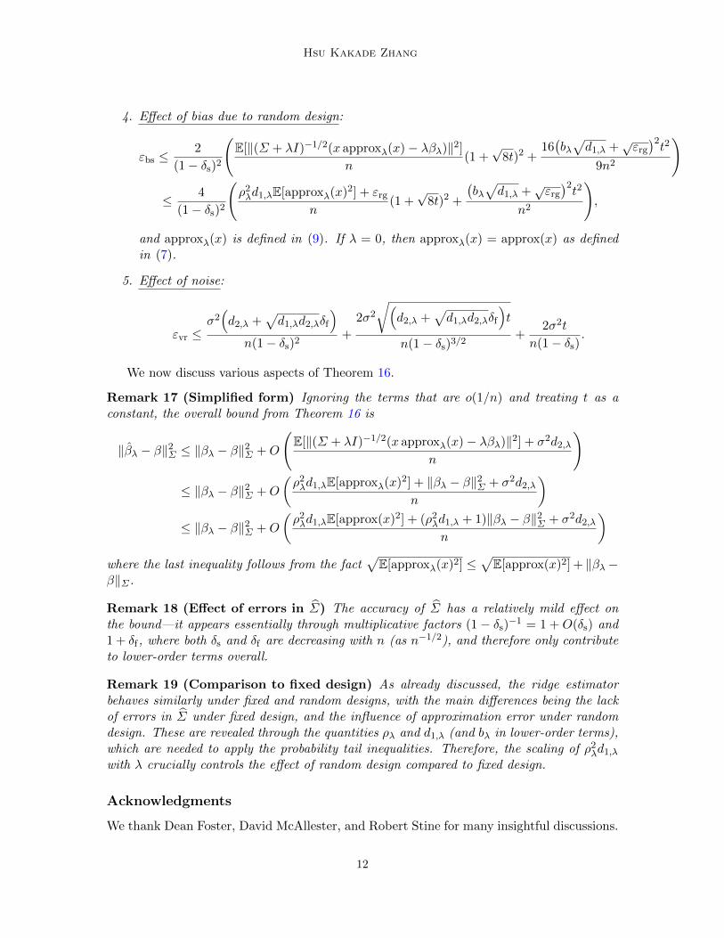
We now discuss various aspects of Theorem 16.

Remark 17 (Simplified form) Ignoring the terms that are o(1/n) and treating t as aconstant, the overall bound from Theorem 16 is

‖βλ − β‖2Σ ≤ ‖βλ − β‖2Σ +O

(E[‖(Σ + λI)−1/2(x approxλ(x)− λβλ)‖2] + σ2d2,λ

n

)

≤ ‖βλ − β‖2Σ +O

(ρ2λd1,λE[approxλ(x)2] + ‖βλ − β‖2Σ + σ2d2,λ

n

)≤ ‖βλ − β‖2Σ +O

(ρ2λd1,λE[approx(x)2] + (ρ2λd1,λ + 1)‖βλ − β‖2Σ + σ2d2,λ

n

)where the last inequality follows from the fact

√E[approxλ(x)2] ≤

√E[approx(x)2] + ‖βλ −

β‖Σ.

Remark 18 (Effect of errors in Σ) The accuracy of Σ has a relatively mild effect onthe bound—it appears essentially through multiplicative factors (1− δs)−1 = 1 + O(δs) and1 + δf , where both δs and δf are decreasing with n (as n−1/2), and therefore only contributeto lower-order terms overall.

Remark 19 (Comparison to fixed design) As already discussed, the ridge estimatorbehaves similarly under fixed and random designs, with the main differences being the lackof errors in Σ under fixed design, and the influence of approximation error under randomdesign. These are revealed through the quantities ρλ and d1,λ (and bλ in lower-order terms),which are needed to apply the probability tail inequalities. Therefore, the scaling of ρ2λd1,λwith λ crucially controls the effect of random design compared to fixed design.

Acknowledgments

We thank Dean Foster, David McAllester, and Robert Stine for many insightful discussions.

12


References

J.-Y. Audibert and O. Catoni. Robust linear least squares regression, 2010a.arXiv:1010.0074.

J.-Y. Audibert and O. Catoni. Robust linear regression through PAC-Bayesian truncation,2010b. arXiv:1010.0072.

A. Caponnetto and E. De Vito. Optimal rates for the regularized least-squares algorithm.Foundations of Computational Mathematics, 7(3):331–368, 2007.

O. Catoni. Statistical Learning Theory and Stochastic Optimization, Lectures on Probabilityand Statistics, Ecole d’Ete de Probabilities de Saint-Flour XXXI – 2001, volume 1851 ofLecture Notes in Mathematics. Springer, 2004.

L. Gyorfi, M. Kohler, A. Kryzak, and H. Walk. A Distribution-Free Theory of Nonpara-metric Regression. Springer, 2004.

A. E. Hoerl. Application of ridge analysis to regression problems. Chemical EngineeringProgress, 58:54–59, 1962.

R. Horn and C. R. Johnson. Matrix Analysis. Cambridge University Press, 1985.

D. Hsu, S. M. Kakade, and T. Zhang. A tail inequality for quadratic forms of subgaussianrandom vectors, 2011. arXiv:1110.2842.

D. Hsu, S. M. Kakade, and T. Zhang. Tail inequalities for sums of random matrices thatdepend on the intrinsic dimension. Electronic Communications in Probability, 17(14):1–13, 2012.

V. Koltchinskii. Local Rademacher complexities and oracle inequalities in risk minimization.The Annals of Statistics, 34(6):2593–2656, 2006.

B. Laurent and P. Massart. Adaptive estimation of a quadratic functional by model selec-tion. The Annals of Statistics, 28(5):1302–1338, 2000.

S. Smale and D.-X. Zhou. Learning theory estimates via integral operators and their ap-proximations. Constructive Approximations, 26:153–172, 2007.

I. Steinwart, D. Hush, and C. Scovel. Optimal rates for regularized least squares regression.In Proceedings of the 22nd Annual Conference on Learning Theory, pages 79–93, 2009.

G. W. Stewart and J.-G. Sun. Matrix Perturbation Theory. Academic Press, 1990.

C. J. Stone. Optimal global rates of convergence for nonparametric regression. Annals ofStatistics, 10:1040–1053, 1982.

T. Zhang. Learning bounds for kernel regression using effective data dimensionality. NeuralComputation, 17:2077–2098, 2005.

13

Hsu Kakade Zhang

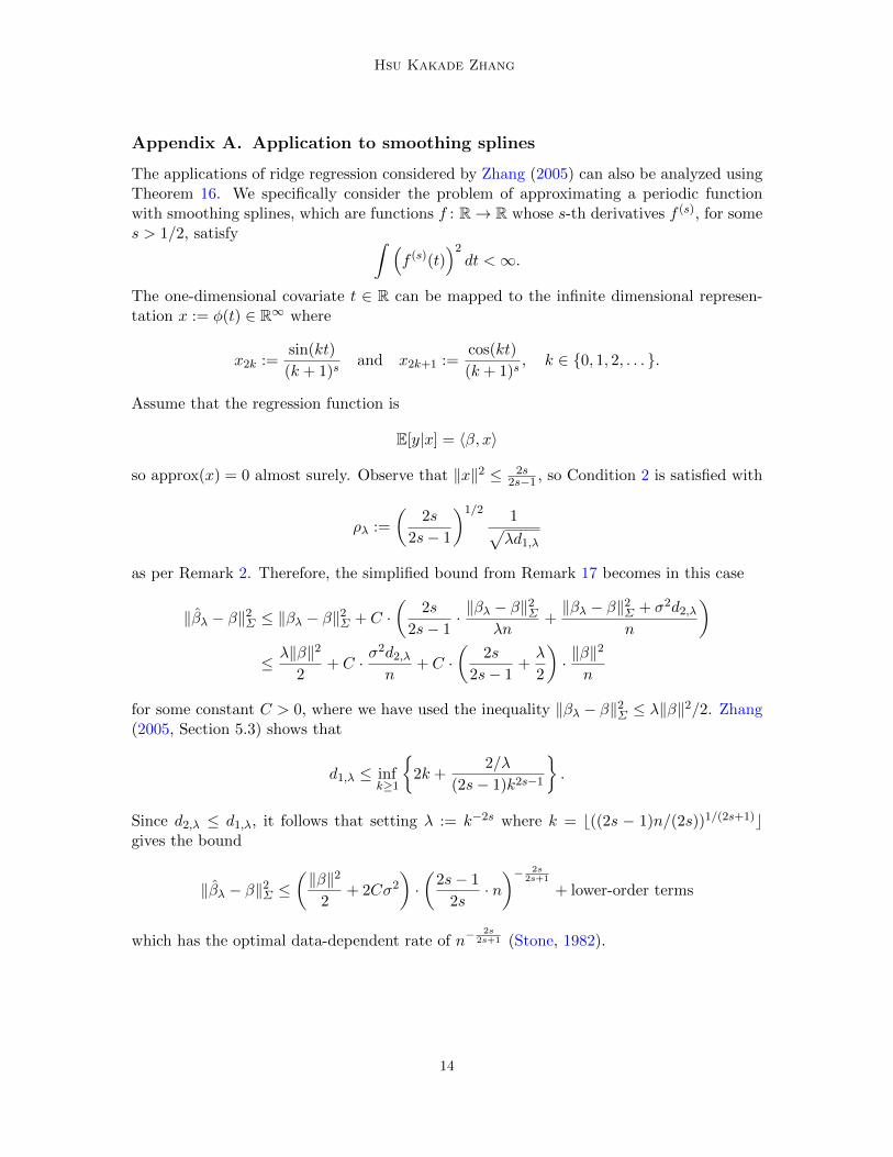
Appendix A. Application to smoothing splines

The applications of ridge regression considered by Zhang (2005) can also be analyzed usingTheorem 16. We specifically consider the problem of approximating a periodic functionwith smoothing splines, which are functions f : R→ R whose s-th derivatives f (s), for somes > 1/2, satisfy ∫ (

f (s)(t))2dt <∞.

The one-dimensional covariate t ∈ R can be mapped to the infinite dimensional represen-tation x := φ(t) ∈ R∞ where

x2k :=sin(kt)

(k + 1)sand x2k+1 :=

cos(kt)

(k + 1)s, k ∈ {0, 1, 2, . . . }.

Assume that the regression function is

E[y|x] = 〈β, x〉

so approx(x) = 0 almost surely. Observe that ‖x‖2 ≤ 2s2s−1 , so Condition 2 is satisfied with

ρλ :=

(2s

2s− 1

)1/2 1√λd1,λ

as per Remark 2. Therefore, the simplified bound from Remark 17 becomes in this case

‖βλ − β‖2Σ ≤ ‖βλ − β‖2Σ + C ·(

2s

2s− 1·‖βλ − β‖2Σ

λn+‖βλ − β‖2Σ + σ2d2,λ

n

)≤ λ‖β‖2

2+ C ·

σ2d2,λn

+ C ·(

2s

2s− 1+λ

2

)· ‖β‖

2

n

for some constant C > 0, where we have used the inequality ‖βλ − β‖2Σ ≤ λ‖β‖2/2. Zhang(2005, Section 5.3) shows that

d1,λ ≤ infk≥1

{2k +

2/λ

(2s− 1)k2s−1

}.

Since d2,λ ≤ d1,λ, it follows that setting λ := k−2s where k = b((2s − 1)n/(2s))1/(2s+1)cgives the bound

‖βλ − β‖2Σ ≤(‖β‖2

2+ 2Cσ2

)·(

2s− 1

2s· n)− 2s

2s+1

+ lower-order terms

which has the optimal data-dependent rate of n−2s

2s+1 (Stone, 1982).

14


Appendix B. Proofs of Theorem 11 and Theorem 16

The proof of Theorem 16 uses the decomposition of ‖βλ− β‖2Σ in Proposition 14, and thenbounds each term using the lemmas proved in this section.

The proof of Theorem 11 omits one term from the decomposition in Proposition 14 dueto the fact that β = βλ when λ = 0; and it uses a slightly simpler argument to handle theeffect of noise (Lemma 28 rather than Lemma 29), which reduces the number of lower-orderterms. Other than these differences, the proof is the same as that for Theorem 16 in thespecial case of λ = 0.

Define

Σλ := Σ + λI, (14)

Σλ := Σ + λI, and (15)

∆λ := Σ−1/2λ (Σ −Σ)Σ

−1/2λ (16)

= Σ−1/2λ (Σλ −Σλ)Σ

−1/2λ .

Recall the basic decomposition from Proposition 14:

‖βλ − β‖2Σ ≤(‖βλ − β‖Σ + ‖βλ − βλ‖Σ + ‖βλ − βλ‖Σ

)2.

Section B.1 first establishes basic properties of β and βλ, which are then used to bound‖βλ − β‖2Σ ; this part is exactly the same as the standard fixed design analysis of ridgeregression. Section B.2 employs probability tail inequalities for the spectral and Frobeniusnorms of random matrices to bound the matrix errors in estimating Σ with Σ. Finally,Section B.3 and Section B.4 bound the contributions of approximation error (in ‖βλ−βλ‖2Σ)

and noise (in ‖βλ−βλ‖2Σ), respectively, using probability tail inequalities for random vectors

as well as the matrix error bounds for Σ.

B.1. Basic properties of β and βλ, and the effect of regularization

Proposition 20 (Normal equations) E[〈w, x〉y] = E[〈w, x〉〈β, x〉] for any w.

Proof It suffices to prove the claim for w = vj . Since E[〈vj , x〉〈vj′ , x〉] = 0 for j′ 6= j, itfollows that E[〈vj , x〉〈β, x〉] =

∑j′ βj′E[〈vj , x〉〈vj′ , x〉] = βjE[〈vj , x〉2] = E[〈vj , x〉y], where

the last equality follows from the definition of β in (2).

Proposition 21 (Excess mean squared error) E[(〈w, x〉−y)2]−E[(〈β, x〉−y)2] = E[〈w−β, x〉2] for any w.

Proof Directly expanding the squares in the expectations reveals that

E[(〈w, x〉 − y)2]− E[(〈β, x〉 − y)2]

= E[〈w, x〉2]− 2E[〈w, x〉y] + 2E[〈β, x〉y]− E[〈β, x〉2]= E[〈w, x〉2]− 2E[〈w, x〉〈β, x〉] + 2E[〈β, x〉〈β, x〉]− E[〈β, x〉2]= E[〈w, x〉2 − 2〈w, x〉〈β, x〉+ 〈β, x〉2]= E[〈w − β, x〉2]

15

Hsu Kakade Zhang

where the third equality follows from Proposition 20.

Proposition 22 (Shrinkage) For any j,

〈vj , βλ〉 =λj

λj + λβj .

Proof Since (Σ + λI)−1 =∑

j(λj + λ)−1vj ⊗ vj ,

〈vj , βλ〉 = 〈vj , (Σ + λI)−1E[xy]〉 =1

λj + λE[〈vj , x〉y] =

λjλj + λ

E[〈vj , x〉y]

〈vj , x〉2=

λjλj + λ

βj .

Proposition 23 (Effect of regularization)

‖β − βλ‖2Σ =∑j

λj

(λjλ + 1)2

β2j .

Proof By Proposition 22,

〈vj , β − βλ〉 = βj −λj

λj + λβj =

λ

λj + λβj .

Therefore,

‖β − βλ‖2Σ =∑j

λj

(λ

λj + λβj

)2

=∑j

λj

(λjλ + 1)2

β2j .

B.2. Effect of errors in Σ

Lemma 24 (Spectral norm error in Σ) Assume Condition 1 and Condition 2 (withparameter ρλ) hold. Pick t > max{0, 2.6− log d1,λ}. With probability at least 1− e−t,

‖∆λ‖ ≤

√4ρ2λd1,λ(log d1,λ + t)

n+

2ρ2λd1,λ(log d1,λ + t)

3n

where ∆λ is defined in (16).

Proof The claim is a consequence of the tail inequality from Lemma 32. First, define

x := Σ−1/2λ x and Σ := Σ

−1/2λ ΣΣ

−1/2λ

16


(where Σλ is defined in (14)), and let

Z := x⊗ x− Σ

= Σ−1/2λ (x⊗ x−Σ)Σ

−1/2λ

so ∆λ = E[Z]. Observe that E[Z] = 0 and

‖Z‖ = max{λmax[Z], λmax[−Z]} ≤ max{‖x‖2, 1} ≤ ρ2λd1,λ

where the second inequality follows from Condition 2. Moreover,

E[Z2] = E[(x⊗ x)2]− Σ2 = E[‖x‖2(x⊗ x)]− Σ2

so

λmax[E[Z2]] ≤ λmax[E[(x⊗ x)2]] ≤ ρ2λd1,λλmax[Σ] ≤ ρ2λd1,λtr(E[Z2]) ≤ tr(E[‖x‖2(x⊗ x)]) ≤ ρ2λd1,λ tr(Σ) = ρ2λd

21,λ.

The claim now follows from Lemma 32 (recall that d1,λ = max{1, d1,λ}).

Lemma 25 (Relative spectral norm error in Σλ) If ‖∆λ‖ < 1 where ∆λ is definedin (16), then

‖Σ1/2λ Σ−1λ Σ

1/2λ ‖ ≤

1

1− ‖∆λ‖

where Σλ is defined in (14) and Σλ is defined in (15).

Proof Observe that

Σ−1/2λ ΣλΣ

−1/2λ = Σ

−1/2λ (Σλ + Σλ −Σλ)Σ

−1/2λ

= I +Σ−1/2λ (Σλ −Σλ)Σ

−1/2λ

= I + ∆λ,

and thatλmin[I + ∆λ] ≥ 1− ‖∆λ‖ > 0

by the assumption ‖∆λ‖ < 1 and Weyl’s theorem (Horn and Johnson, 1985, Theorem 4.3.1).Therefore

‖Σ1/2λ Σ−1λ Σ

1/2λ ‖ = λmax[(Σ

−1/2λ ΣλΣ

−1/2λ )−1] = λmax[(I+∆λ)−1] =

1

λmin[I + ∆λ]≤ 1

1− ‖∆‖.

17

Hsu Kakade Zhang

Lemma 26 (Frobenius norm error in Σ) Assume Condition 1 and Condition 2 (withparameter ρλ) hold. Pick any t > 0. With probability at least 1− e−t,

‖∆λ‖F ≤

√E[‖Σ−1/2λ x‖4]− d2,λ

n(1 +

√8t) +

4√ρ4λd

21,λ + d2,λt

3n

≤

√ρ2λd

21,λ − d2,λn

(1 +√

8t) +4√ρ4λd

21,λ + d2,λt

3n

where ∆λ is defined in (16).

Proof The claim is a consequence of the tail inequality in Lemma 31. As in the proof

of Lemma 24, define x := Σ−1/2λ x and Σ := Σ

−1/2λ ΣΣ

−1/2λ , and let Z := x ⊗ x − Σ so

∆λ = E[Z]. Now endow the space of self-adjoint linear operators with the inner productgiven by 〈A,B〉F := tr(AB), and note that this inner product induces the Frobenius norm‖M‖F = 〈M,M〉F. Observe that E[Z] = 0 and

‖Z‖2F = 〈x⊗ x− Σ, x⊗ x− Σ〉F= 〈x⊗ x, x⊗ x〉F − 2〈x⊗ x, Σ〉F + 〈Σ, Σ〉F= ‖x‖4 − 2‖x‖2

Σ+ tr(Σ2)

= ‖x‖4 − 2‖x‖2Σ

+ d2,λ

≤ ρ4λd21,λ + d2,λ

where the inequality follows from Condition 2. Moreover,

E[‖Z‖2F] = E[〈x⊗ x, x⊗ x〉F]− 〈Σ, Σ〉F= E[‖x‖4]− d2,λ≤ ρ2λd1,λE[‖x‖2]− d2,λ= ρ2λd

21,λ − d2,λ

where the inequality again uses Condition 2. The claim now follows from Lemma 31.

B.3. Effect of approximation error

Lemma 27 (Effect of approximation error) Assume Condition 1, Condition 2 (withparameter ρλ), and Condition 4 (with parameter bλ) hold. Pick any t > 0. If ‖∆λ‖ < 1where ∆λ is defined in (16), then

‖βλ − βλ‖Σ ≤1

1− ‖∆λ‖‖E[x approxλ(x)− λβλ]‖Σ−1

λ

18


where βλ is defined in (13), βλ is defined in (8), approxλ(x) is defined in (9), and Σλ isdefined in (14). Moreover, with probability at least 1− e−t,

‖E[x approxλ(x)− λβλ]‖Σ−1λ

≤

√E[‖Σ−1/2λ (x approxλ(x)− λβλ)‖2]

n(1 +

√8t) +

4(bλ√d1,λ + ‖β − βλ‖Σ)t

3n

≤

√2(ρ2λd1,λE[approxλ(x)2] + ‖β − βλ‖2Σ)

n(1 +

√8t) +

4(bλ√d1,λ + ‖β − βλ‖Σ)t

3n.

Proof By the definitions of βλ and βλ,

βλ − βλ = Σ−1λ

(E[xE[y|x]]− Σλβλ

)= Σ

−1/2λ (Σ

1/2λ Σ−1λ Σ

1/2λ )Σ

−1/2λ

(E[x(approx(x) + 〈β, x〉)]− Σβλ − λβλ

)= Σ

−1/2λ (Σ

1/2λ Σ−1λ Σ

1/2λ )Σ

−1/2λ

(E[x(approx(x) + 〈β, x〉 − 〈βλ, x〉)]− λβλ

)= Σ

−1/2λ (Σ

1/2λ Σ−1λ Σ

1/2λ )Σ

−1/2λ

(E[x approxλ(x)− λβλ]

).

Therefore, using the sub-multiplicative property of the spectral norm,

‖βλ − βλ‖Σ ≤ ‖Σ1/2Σ−1/2λ ‖‖Σ1/2

λ Σ−1λ Σ1/2λ ‖‖E[x approxλ(x)− λβλ]‖Σ−1

λ

≤ 1

1− ‖∆λ‖‖E[x approxλ(x)− λβλ]‖Σ−1

λ

where the second inequality follows from Lemma 25 and because

‖Σ1/2Σ−1/2λ ‖2 = λmax[Σ

−1/2λ ΣΣ

−1/2λ ] = max

i

λiλi + λ

≤ 1.

The second part of the claim is a consequence of the tail inequality in Lemma 31. Observethat E[x approx(x)] = E[x(E[y|x]−〈β, x〉)] = 0 by Proposition 20, and that E[x〈β−βλ, x〉]−λβλ = Σβ − (Σ + λI)βλ = 0. Therefore,

E[Σ−1/2λ (x approxλ(x)− λβλ)] = Σ

−1/2λ E[x(approx(x) + 〈β − βλ, x〉)− λβλ] = 0.

Moreover, by Proposition 22 and Proposition 23,

‖λΣ−1/2λ βλ‖2 =∑j

λ2

λj + λ〈vj , βλ〉2

=∑j

λ2

λj + λ

(λj

λj + λβj

)2

≤∑j

λ2

λj + λ

(λj

λj + λ

)β2j

=∑j

λj

(λjλ + 1)2

β2j

= ‖β − βλ‖2Σ . (17)

19

Hsu Kakade Zhang

Combining the inequality from (17) with Condition 4 and the triangle inequality, it followsthat

‖Σ−1/2λ (x approxλ(x)− λβλ)‖ ≤ ‖Σ−1/2λ x approxλ(x)‖+ ‖λΣ−1/2λ βλ‖≤ bλ

√d1,λ + ‖β − βλ‖Σ .

Finally, by the triangle inequality, the fact (a+ b)2 ≤ 2(a2 + b2), the inequality from (17),and Condition 2,

E[‖Σ−1/2λ (x approxλ(x)− λβλ)‖2] ≤ 2(E[‖Σ−1/2λ x approxλ(x)‖2] + ‖βλ − β‖2Σ)

≤ 2(ρ2λd1,λE[approxλ(x)2] + ‖βλ − β‖2Σ).

The claim now follows from Lemma 31.

B.4. Effect of noise

Lemma 28 (Effect of noise, λ = 0) Assume the dimension of the covariate space is d <∞ and that λ = 0. Assume Condition 3 (with parameter σ) holds. Pick any t > 0. Withprobability at least 1− e−t, either ‖∆0‖ ≥ 1, or

‖∆0‖ < 1 and ‖β0 − β0‖2Σ ≤1

1− ‖∆0‖· σ

2(d+ 2√dt+ 2t)

n,

where ∆0 is defined in (16).

Proof Observe that

‖β0 − β0‖2Σ ≤ ‖Σ1/2Σ−1/2‖2‖β0 − β0‖2Σ = ‖Σ1/2Σ−1Σ1/2‖‖β0 − β0‖2Σ ;

and if ‖∆0‖ < 1, then ‖Σ1/2Σ−1Σ1/2‖ ≤ 1/(1− ‖∆0‖) by Lemma 25.Let ξ := (noise(x1),noise(x2), . . . ,noise(xn)) be the random vector whose i-th compo-

nent is noise(xi) = yi − E[yi|xi]. By the definition of β0 and β0

‖β0 − β0‖2Σ = ‖Σ−1/2E[x(y − E[y|x])]‖2 = ξ>Kξ

where K ∈ Rn×n is the symmetric matrix whose (i, j)-th entry is Ki,j := n−2〈Σ−1/2xi, Σ−1/2xj〉.Note that the non-zero eigenvalues of K are the same as those of

1

nE[(Σ−1/2x)⊗ (Σ−1/2x)

]=

1

nΣ−1/2ΣΣ−1/2 =

1

nI.

By Lemma 30, with probability at least 1− e−t (conditioned on x1, x2, . . . , xn),

ξ>Kξ ≤ σ2(tr(K) + 2

√tr(K2)t+ 2λmax(K)t) =

σ2(d+ 2√dt+ 2t)

n.

The claim follows.

20


Lemma 29 (Effect of noise, λ ≥ 0) Assume Condition 1 and Condition 3 (with param-eter σ) hold. Pick any t > 0. Let K be the n × n symmetric matrix whose (i, j)-th entryis

Ki,j :=1

n2〈Σ1/2Σ−1λ xi, Σ

1/2Σ−1λ xj〉

where Σλ is defined in (15). With probability at least 1− e−t,

‖βλ − βλ‖2Σ ≤ σ2(tr(K) + 2√

tr(K)λmax(K)t+ 2λmax(K)t).

Moreover, if ‖∆λ‖ < 1 where ∆λ is defined in (16), then

λmax(K) ≤ 1

n(1− ‖∆λ‖)and tr(K) ≤

d2,λ +√d2,λ‖∆λ‖2F

n(1− ‖∆λ‖)2.

Proof Let ξ := (noise(x1), noise(x2), . . . ,noise(xn)) be the random vector whose i-th com-ponent is noise(xi) = yi − E[yi|xi]. By the definition of βλ, βλ, and K,

‖βλ − βλ‖2Σ = ‖Σ−1λ E[x(y − E[y|x])]‖2Σ = ξ>Kξ.

By Lemma 30, with probability at least 1− e−t (conditioned on x1, x2, . . . , xn),

ξ>Kξ ≤ σ2(tr(K) + 2√

tr(K2)t+ 2λmax(K)t)

≤ σ2(tr(K) + 2√

tr(K)λmax(K)t+ 2λmax(K)t)

where the second inequality follows from von Neumann’s theorem (Horn and Johnson, 1985,page 423).

Note that the non-zero eigenvalues of K are the same as that of

1

nE[(Σ1/2Σ−1λ x)⊗ (Σ1/2Σ−1λ x)

]=

1

nΣ1/2Σ−1λ ΣΣ−1λ Σ1/2.

To bound λmax(K), observe that by the sub-multiplicative property of the spectral normand Lemma 25,

nλmax(K) = ‖Σ1/2Σ−1λ Σ1/2‖2

≤ ‖Σ1/2Σ−1/2λ ‖2‖Σ1/2

λ Σ−1/2λ ‖2‖Σ−1/2λ Σ1/2‖2

≤ ‖Σ1/2λ Σ

−1/2λ ‖2

= ‖Σ1/2λ Σ−1λ Σ

1/2λ ‖

≤ 1

1− ‖∆λ‖.

To bound tr(K), first define the λ-whitened versions of Σ, Σ, and Σλ:

Σw := Σ−1/2λ ΣΣ

−1/2λ

Σw := Σ−1/2λ ΣΣ

−1/2λ

Σλ,w := Σ−1/2λ ΣλΣ

−1/2λ .

21

Hsu Kakade Zhang

Using these definitions with the cycle property of the trace,

n tr(K) = tr(Σ1/2Σ−1λ ΣΣ−1λ Σ1/2)

= tr(Σ−1λ ΣΣ−1λ Σ)

= tr(Σ−1λ,wΣwΣ−1λ,wΣw).

Let {λj [M ]} denote the eigenvalues of a linear operator M . By von Neumann’s theo-rem (Horn and Johnson, 1985, page 423),

tr(Σ−1λ,wΣwΣ−1λ,wΣw) ≤

∑j

λj [Σ−1λ,wΣwΣ

−1λ,w]λj [Σw]

and by Ostrowski’s theorem (Horn and Johnson, 1985, Theorem 4.5.9),

λj [Σ−1λ,wΣwΣ

−1λ,w] ≤ λmax[Σ−2λ,w]λj [Σw].

Therefore

tr(Σ−1λ,wΣwΣ−1λ,wΣw) ≤ λmax[Σ−2λ,w]

∑j

λj [Σw]λj [Σw]

≤ 1

(1− ‖∆λ‖)2∑j

λj [Σw]λj [Σw]

=1

(1− ‖∆λ‖)2∑j

(λj [Σw]2 + (λj [Σw]− λj [Σw])λj [Σw]

)

≤ 1

(1− ‖∆λ‖)2

∑j

λj [Σw]2 +

√∑j

(λj [Σw]− λj [Σw])2√∑

j

λj [Σw]2

=

1

(1− ‖∆λ‖)2

d2,λ +

√∑j

(λj [Σw]− λj [Σw])2√d2,λ

≤ 1

(1− ‖∆λ‖)2(d2,λ + ‖Σw −Σw‖F

√d2,λ

)=

1

(1− ‖∆λ‖)2(d2,λ + ‖∆λ‖F

√d2,λ

)where the second inequality follows from Lemma 25, the third inequality follows fromCauchy-Schwarz, and the fourth inequality follows from Mirsky’s theorem (Stewart andSun, 1990, Corollary 4.13).

Appendix C. Probability tail inequalities

The following probability tail inequalities are used in our analysis. These specific inequalitieswere chosen in order to satisfy the general conditions setup in Section 2.4; however, our

22


analysis can specialize or generalize with the availability of other tail inequalities of thesesorts.

The first tail inequality is for positive semidefinite quadratic forms of a subgaussianrandom vector. It generalizes a standard tail inequality for Gaussian random vectors basedon linear combinations of χ2 random variables (Laurent and Massart, 2000). We give theproof for completeness.

Lemma 30 (Quadratic forms of a subgaussian random vector; Hsu et al., 2011)Let ξ be a random vector taking values in Rn such that for some c ≥ 0,

E[exp(〈u, ξ〉)] ≤ exp(c‖u‖2/2), ∀u ∈ Rn.

For all symmetric positive semidefinite matrices K � 0, and all t > 0,

Pr

[ξ>Kξ > c

(tr(K) + 2

√tr(K2)t+ 2‖K‖t

)]≤ e−t.

Proof Let z ∈ Rn be a vector of n i.i.d. standard normal random variables (independentof ξ). For any τ ≥ 0 and λ ≥ 0, let η := cλ2/2, so

E[exp(λ〈z,K1/2ξ〉)

]≥ E

[exp(λ〈z,K1/2ξ〉)|‖K1/2ξ‖2 > c(tr(K) + τ)

]· Pr[‖K1/2ξ‖2 > c(tr(K) + τ)

]≥ exp(λ2c(tr(K) + τ)/2) · Pr

[‖K1/2ξ‖2 > c(tr(K) + τ)

]= exp(η(tr(K) + τ)) · Pr

[‖K1/2ξ‖2 > c(tr(K) + τ)

](18)

since E[exp(〈u, z〉)] = exp(‖u‖2/2) for any u ∈ Rn. Moreover, by independence of ξ and z,


]= E

[E[exp(λ〈K1/2z, ξ〉)|z

]]≤ E

[exp(cλ2‖K1/2z‖2/2)

]= E

[exp(η‖K1/2z‖2)

].

Since K is symmetric and positive semidefinite, K = V DV > for some orthogonal ma-trix V = [u1|u2| · · · |ur] and diagonal matrix D = diag(ρ1, ρ2, . . . , ρr), where r is the rankof K. By rotational symmetry, the vector V >z is equal in distribution to a vector ofr i.i.d. standard normal random variables q1, q2, . . . , qr, and ‖K1/2z‖2 = ‖D1/2V >z‖2 =ρ1q

21 + ρ2q

22 + · · ·+ ρrq

2r . Therefore,


]≤ E

[exp(η‖K1/2z‖2)

]= E

[exp(η(ρ1q

21 + ρ2q

22 + · · ·+ ρrq

2r ))]. (19)

Combining (18) and (19) gives

Pr[‖K1/2ξ‖2 > c(tr(K) + τ)

]≤ exp(−η(tr(K) + τ)) · E

[exp(η(ρ1q

21 + ρ2q

22 + · · ·+ ρrq

2r ))].

The expectation on the right-hand side is the moment generating function for a linearcombination of r independent χ2 random variables, each with one degree of freedom. Sincetr(K) = ρ1 + ρ2 + · · ·+ ρr, tr(K2) = ρ21 + ρ22 + · · ·+ ρ2r , and ‖K‖ = max{ρ1, ρ2, . . . , ρr}, the

23

Hsu Kakade Zhang

conclusion follows from standard facts about χ2 random variables (Laurent and Massart,2000):

Pr[‖K1/2ξ‖2 > c(tr(K) + τ)

]≤ exp

(−tr(K2)

2‖K‖· h1(‖K‖τtr(K2)

))where h1(a) := 1 + a−

√1 + 2a.

The next lemma is a tail inequality for sums of bounded random vectors; it is a standardapplication of Bernstein’s inequality.

Lemma 31 (Vector Bernstein bound; see, e.g., Hsu et al., 2011) Let x1, x2, . . . , xnbe independent random vectors such that

n∑i=1

E[‖xi‖2] ≤ v and ‖xi‖ ≤ r

for all i = 1, 2, . . . , n, almost surely. Let s := x1 + x2 + · · ·+ xn. For all t > 0,

Pr[‖s‖ >

√v(1 +

√8t) + (4/3)rt

]≤ e−t

The last tail inequality concerns the spectral accuracy of an empirical second momentmatrix.

Lemma 32 (Matrix Bernstein bound; Hsu et al., 2012) Let X be a random matrix,and r > 0, v > 0, and k > 0 be such that, almost surely,

E[X] = 0, λmax[X] ≤ r, λmax[E[X2]] ≤ v, tr(E[X2]) ≤ vk.

If X1, X2, . . . , Xn are independent copies of X, then for any t > 0,

Pr

[λmax

[1

n

n∑i=1

Xi

]>

√2vt

n+rt

3n

]≤ kt(et − t− 1)−1.

If t ≥ 2.6, then t(et − t− 1)−1 ≤ e−t/2.

24

random design analysis of ridge regressiondjhsu/papers/ridge-colt.pdfrandom design analysis of ridge...

Documents