random e ects anova - statpowerstatpower.net/content/311/lecture notes/randomeffects.pdf · random...

Random Effects ANOVA

James H. Steiger

Department of Psychology and Human DevelopmentVanderbilt University

James H. Steiger (Vanderbilt University) 1 / 29

Random Effects ANOVA1 Introduction

2 A One-Way Random Effects ANOVA

The Basic Model

Calculations

Expected Mean Squares and F Test

3 Two-Way Model with Both Effects Random

4 A Typical Two-Way Model with One Random Effect

Factor B

Factor A

The Basic Model

Computations and Expected Mean Squares

5 Two-Way Mixed Model ANOVA: An Example


Introduction

Introduction

So far, in our coverage of ANOVA, we have dealt only with the case offixed-effects models.

With fixed-effects factors, the effects of the different levels of theindependent variable are treated as fixed constants to be estimated.

In this module, we introduce the idea of a random-effect factor. Thetreatment effects for random effects factors are treated as randomvariables, or, equivalently, random samples from a population of possibletreatment effects.

When models include random effects, the Expected Mean Squares willoften differ from the same model with fixed effects.

In most cases, this will affect how F -tests are performed, and thedistribution of the F -statistic and its degrees of freedom.


A One-Way Random Effects ANOVA


Suppose you are interested in the natural degree of variation in sodiumcontent across brands of beer.

There are hundreds of brands of beer being sold in the U.S., and you onlyhave time to test 8.

You select your 8 brands randomly from a list of all brands available, andyou test 6 bottles of beer for each brand.




Although we can visualize an “effect” for each brand, we recognize thatthis effect need not be conceptualized as a fixed value — in an importantsense, the effect of the first brand is a random variable, since that brandwas sampled from a larger set.

If we were only interested in generalizing to the 8 brands in the study, wecould choose to regard the effect of each beer as a fixed constant.

But because we randomly sampled the beer brands from a largerpopulation, we actually can generalize back to the entire population. Let’ssee how.


A One-Way Random Effects ANOVA The Basic Model

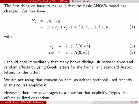
The first thing we have to realize is that the basic ANOVA model haschanged. We now have

Yij = µj + εij

= µ+ αj + εij 1 ≤ i ≤ n, 1 ≤ j ≤ a (1)

with

εij ∼ i.i.d. N(0, σ2e ) (2)

αij ∼ i.i.d N(0, σ2A) (3)

I should note immediately that many books distinguish between fixed andrandom effects by using Greek letters for the former and standard Arabicletters for the latter.

We are not using that convention here, as neither textbook used recentlyin this course employs it.

However, there are advantages to a notation that explicitly “types” itseffects as fixed or random.



A One-Way Random Effects ANOVAThe Basic Model

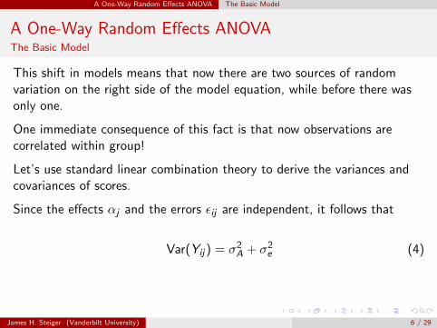
This shift in models means that now there are two sources of randomvariation on the right side of the model equation, while before there wasonly one.

One immediate consequence of this fact is that now observations arecorrelated within group!

Let’s use standard linear combination theory to derive the variances andcovariances of scores.

Since the effects αj and the errors εij are independent, it follows that

Var(Yij) = σ2A + σ2

e (4)




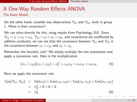
On the other hand, consider two observations Y11 and Y21, both in group1. What is their covariance?

We can solve directly for this, using results from Psychology 310. SinceY11 = µ+α1 + ε11, Y21 = µ+α1 + ε21, and covariances are unaffected byadditive constants, we can see that the covariance between Y11 and Y21 isthe covariance between α1 + ε11 and α1 + ε21.

Remember the heuristic rule? We simply multiply the two expressions andapply a conversion rule. Here is the multiplication.

(α1 + ε11)(α1 + ε21) = α21 + ε11ε21 + α1ε11 + α1ε21 (5)

Next we apply the conversion rule

Cov(Y11,Y21) = Var(α1) + Cov(ε11, ε21) + Cov(α1, ε11) + Cov(α1, ε21)

= σ2A + 0 + 0 + 0

= σ2A (6)




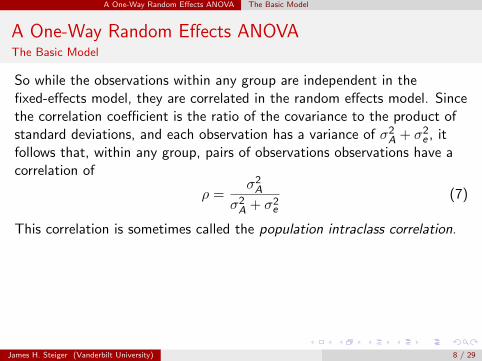
So while the observations within any group are independent in thefixed-effects model, they are correlated in the random effects model. Sincethe correlation coefficient is the ratio of the covariance to the product ofstandard deviations, and each observation has a variance of σ2

A + σ2e , it

follows that, within any group, pairs of observations observations have acorrelation of

ρ =σ2A

σ2A + σ2

e

(7)

This correlation is sometimes called the population intraclass correlation.


A One-Way Random Effects ANOVA Calculations

A One-Way Random Effects ANOVACalculations

We are very fortunate, in that the sums of squares for the random effectsmodel are calculated in exactly the same way they are calculated for thefixed effects model.


A One-Way Random Effects ANOVA Expected Mean Squares and F Test

A One-Way Random Effects ANOVAExpected Mean Squares and F Test

Remember that earlier in the course, I mentioned that ultimately ExpectedMean Squares would play an important role in deciding how to perform anF test on a particular model. We have almost reached that point. Noticein the table below that the expected mean squares for the random effectsmodel are almost identical to those for the fixed effects model.




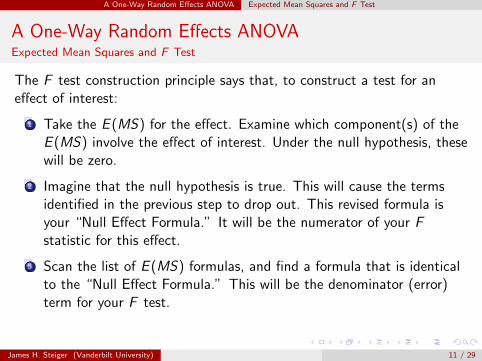
The F test construction principle says that, to construct a test for aneffect of interest:

1 Take the E (MS) for the effect. Examine which component(s) of theE (MS) involve the effect of interest. Under the null hypothesis, thesewill be zero.

2 Imagine that the null hypothesis is true. This will cause the termsidentified in the previous step to drop out. This revised formula isyour “Null Effect Formula.” It will be the numerator of your Fstatistic for this effect.

3 Scan the list of E (MS) formulas, and find a formula that is identicalto the “Null Effect Formula.” This will be the denominator (error)term for your F test.




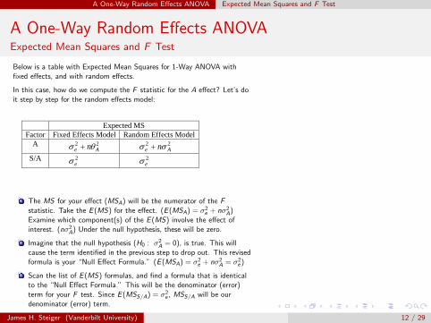
Below is a table with Expected Mean Squares for 1-Way ANOVA withfixed effects, and with random effects.

In this case, how do we compute the F statistic for the A effect? Let’s doit step by step for the random effects model:

Expected MS Factor Fixed Effects Model Random Effects Model

A 2 2Ae nσ θ+ 2 2

Ae nσ σ+ S/A 2

eσ 2eσ

1 The MS for your effect (MSA) will be the numerator of the Fstatistic. Take the E (MS) for the effect. (E (MSA) = σ2

e + nσ2A)

Examine which component(s) of the E (MS) involve the effect ofinterest. (nσ2

A) Under the null hypothesis, these will be zero.

2 Imagine that the null hypothesis (H0 : σ2A = 0), is true. This will

cause the term identified in the previous step to drop out. This revisedformula is your “Null Effect Formula.” (E (MSA) = σ2

e + nσ2A = σ2

e )

3 Scan the list of E (MS) formulas, and find a formula that is identicalto the “Null Effect Formula.” This will be the denominator (error)term for your F test. Since E (MSS/A) = σ2

e , MSS/A will be ourdenominator (error) term.




You can quickly see that the F test for the A effect in the fixed effectsmodel also uses MSS/A as the error term.

Thus, by our F -test construction principle, the F statistic is computed asMSA/MSS/A in both models.

With the F test computed the same way, one might be tempted to thinkthat it has the same distribution. It does when the null hypothesis is true,but it does not when the null hypothesis is false.




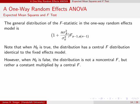
The general distribution of the F -statistic in the one-way random effectsmodel is

(1 +nσ2

A

σ2e

)Fa−1,a(n−1)

Note that when H0 is true, the distribution has a central F distributionidentical to the fixed effects model.

However, when H0 is false, the distribution is not a noncentral F , butrather a constant multiplied by a central F .


Two-Way Model with Both Effects Random

Two-Way Model with Both Effects Random

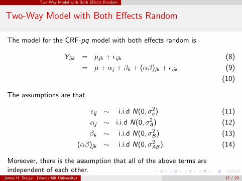
The model for the CRF-pq model with both effects random is

Yijk = µjk + εijk (8)

= µ+ αj + βk + (αβ)jk + εijk (9)

(10)

The assumptions are that

εij ∼ i.i.d N(0, σ2e ) (11)

αj ∼ i.i.d N(0, σ2A) (12)

βk ∼ i.i.d N(0, σ2B) (13)

(αβ)jk ∼ i.i.d N(0, σ2AB). (14)

Moreover, there is the assumption that all of the above terms areindependent of each other.


A Typical Two-Way Model with One Random Effect

A Typical Two-Way Model with One Random Effect

Suppose we were interested in the effect of a type of Study Program onstudent learning, but we were also interested in the effect of the schoolenvironment.

We go to a large local school district and select 4 schools at random froma list of potential participating schools.

Next, we sample 10 student volunteers from each school, and randomlyassign them to two training methods, “Computer” and “Standard.” In thisdesign, Study Program is Factor A, and School is Factor B.


A Typical Two-Way Model with One Random Effect Factor B

A Typical Two-Way Model with One Random EffectFactor B

Consider Factor B (School), and how we might model it. Actually, wehave a choice of models that we might apply to this situation:

1 One model views the 4 selected schools as the only schools of interest.Since these are the only schools of interest, the effects of school 1, forexample, on learning can be viewed as a fixed quantity to beestimated. In this model, the school factor, factor B, is a fixed effect.

2 The other model, probably more in line with our substantive goal,views the schools as simply a sample from a larger population ofinterest. In this model, we can make inferences about the entirepopulation of schools, and school is a random effect.


A Typical Two-Way Model with One Random Effect Factor A

A Typical Two-Way Model with One Random EffectFactor A

Factor A, in this study, is Study Program.

There are two study programs, and we are interested in comparing thesetwo specific programs.

These programs have not been sampled from some population of interest.Consequently, we treat Factor A as a fixed-effects factor.


A Typical Two-Way Model with One Random Effect The Basic Model

A Typical Two-Way Model with One Random EffectThe Basic Model

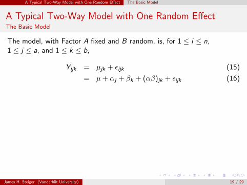
The model, with Factor A fixed and B random, is, for 1 ≤ i ≤ n,1 ≤ j ≤ a, and 1 ≤ k ≤ b,

Yijk = µjk + εijk (15)

= µ+ αj + βk + (αβ)jk + εijk (16)


A Typical Two-Way Model with One Random Effect The Basic Model

A Typical Two-Way Model with One Random EffectThe Basic Model

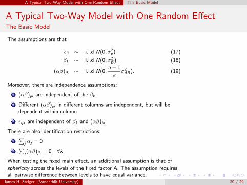
The assumptions are that

εij ∼ i.i.d N(0, σ2e ) (17)

βk ∼ i.i.d N(0, σ2B) (18)

(αβ)jk ∼ i.i.d N(0,a− 1

aσ2AB). (19)

Moreover, there are independence assumptions:

1 (αβ)jk are independent of the βk .

2 Different (αβ)jk in different columns are independent, but will bedependent within column.

3 εijk are independent of βk and (αβ)jk

There are also identification restrictions:

1∑

j αj = 0

2∑

j(αβ)jk = 0 ∀k

When testing the fixed main effect, an additional assumption is that ofsphericity across the levels of the fixed factor A. The assumption requiresall pairwise difference between levels to have equal variance.


A Typical Two-Way Model with One Random Effect Computations and Expected Mean Squares

A Typical Two-Way Model with One Random EffectComputations and Expected Mean Squares

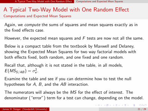
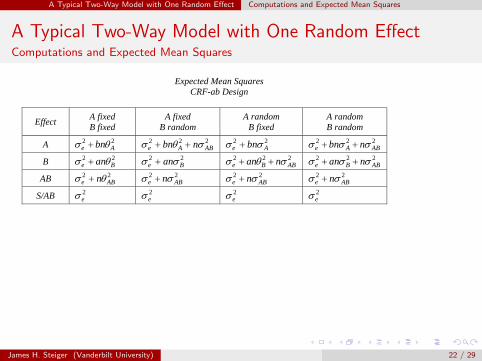
Again, we compute the sums of squares and mean squares exactly as inthe fixed effects case.

However, the expected mean squares and F tests are now not all the same.

Below is a compact table from the textbook by Maxwell and Delaney,showing the Expected Mean Squares for two way factorial models withboth effects fixed, both random, and one fixed and one random.

Recall that, although it is not stated in the table, in all models,E (MSS/AB) = σ2

e .

Examine the table and see if you can determine how to test the nullhypotheses for A, B, and the AB interaction.

The numerators will always be the MS for the effect of interest. Thedenominator (“error”) term for a test can change, depending on the model.




Expected Mean Squares CRF-ab Design

Effect A fixed B fixed

A fixed B random

A random B fixed

A random B random

A 2 2e Abn 2 2 2

e A ABnbn 2 2e Abn 2 2 2

e A ABnbn

B 2 2e Ban 2 2

e Ban 2 2 2e B ABnan 2 2 2

e B ABnan

AB 2 2e ABn 2 2

e ABn 2 2e ABn 2 2

e ABn

S/AB 2e

2e

2e

2e






A fixed B random

A random B fixed

A random B random

A 2 2e Abn 2 2 2


e A ABnbn

B 2 2e Ban 2 2


e B ABnan

AB 2 2e ABn 2 2

e ABn 2 2e ABn 2 2

e ABn

S/AB 2e

2e

2e

2e

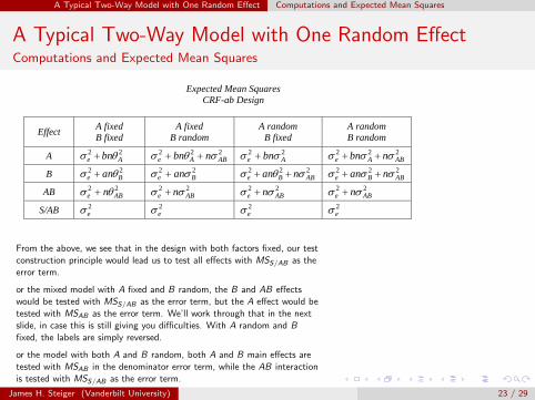
From the above, we see that in the design with both factors fixed, our testconstruction principle would lead us to test all effects with MSS/AB as theerror term.

or the mixed model with A fixed and B random, the B and AB effectswould be tested with MSS/AB as the error term, but the A effect would betested with MSAB as the error term. We’ll work through that in the nextslide, in case this is still giving you difficulties. With A random and Bfixed, the labels are simply reversed.

or the model with both A and B random, both A and B main effects aretested with MSAB in the denominator error term, while the AB interactionis tested with MSS/AB as the error term.






A fixed B random

A random B fixed

A random B random

A 2 2e Abn 2 2 2


e A ABnbn

B 2 2e Ban 2 2


e B ABnan

AB 2 2e ABn 2 2

e ABn 2 2e ABn 2 2

e ABn

S/AB 2e

2e

2e

2e

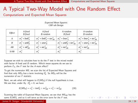
Suppose we wish to calculate how to do the F test in the mixed modelwith factor A fixed and B random. Which mean squares do we use toperform FA, the F test for the A main effect?

To get the numerator MS , we scan the list of Expected Mean Squares andfind that only MSA has a term involving θ2

A. So MSA will be thenumerator of our F statistic.

Next, we ask what will happen to E (MSA) if the null hypothesis is true.We see that, under H0 : θ2

A = 0, we have

E (MSA) = σ2e + bnθ2

A + nσ2AB = σ2

e + nσ2AB (20)

Scanning the table of Expected Mean Squares, we see that MSAB has thesame E (MS), and so it will serve as the error term for the F test.


Two-Way Mixed Model ANOVA: An Example


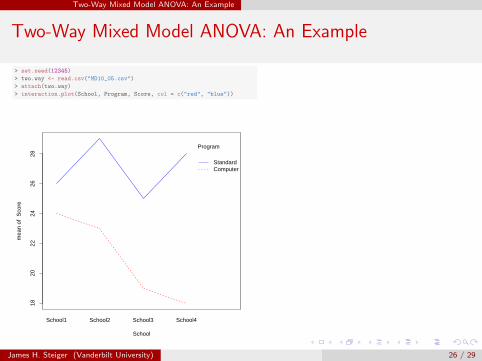
Maxwell and Delaney (p.481, Table 10.5) present data for a 2-way ANOVAexploring the effects of Program and School on ACT Score. The data arein a file called MD10 05.txt.

Reading in the file, and examining the interaction plot, we see definitesigns of a main effect for Program.




> set.seed(12345)

> two.way <- read.csv("MD10_05.csv")

> attach(two.way)

> interaction.plot(School, Program, Score, col = c("red", "blue"))

1820

2224

2628

School

mea

n of

Sco

re

School1 School2 School3 School4

Program

StandardComputer




Unfortunately, unlike some commercial software, R does not currentlypossess a facility whereby one can indicate whether an effect is fixed orrandom, and have the correct F statistic generated automatically.

Some user intervention is required, although one may easily write afunction to automate the process for simple designs such as a two-way.

Since the computations for the sums of squares and mean squares areidentical for fixed, random, and mixed effects models, we need onlyperform the computations the standard way, and then change the F testsonly for those effects with a different error term than the standardfixed-effects model.

What that boils down to, for a two-way completely randomized factorialdesign, is:

1 If the model is mixed, the fixed effect F test is performed using theinteraction mean square as the (denominator) error term, and

2 If the model has random effects for both main effects, then both maineffect F tests are performed using the interaction mean square as theerror term.

We demonstrate the calculations for the current example on the next slide.Notice how the code performs the standard fixed-effects ANOVA, thenreplaces the test for the Program factor with the correct F statistic andreconstitutes the table.




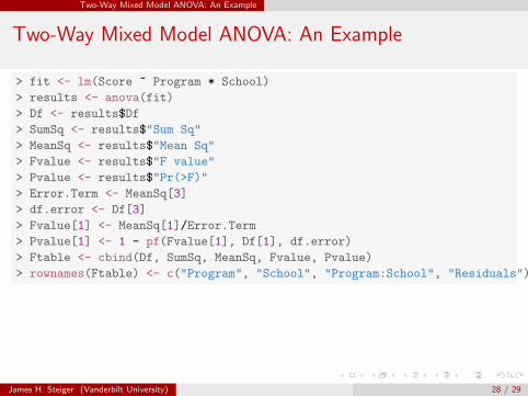
> fit <- lm(Score ~ Program * School)

> results <- anova(fit)

> Df <- results$Df

> SumSq <- results$"Sum Sq"

> MeanSq <- results$"Mean Sq"

> Fvalue <- results$"F value"

> Pvalue <- results$"Pr(>F)"

> Error.Term <- MeanSq[3]

> df.error <- Df[3]

> Fvalue[1] <- MeanSq[1]/Error.Term

> Pvalue[1] <- 1 - pf(Fvalue[1], Df[1], df.error)

> Ftable <- cbind(Df, SumSq, MeanSq, Fvalue, Pvalue)

> rownames(Ftable) <- c("Program", "School", "Program:School", "Residuals")




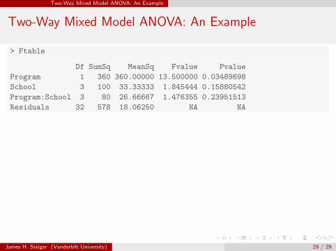
> Ftable

Df SumSq MeanSq Fvalue Pvalue

Program 1 360 360.00000 13.500000 0.03489698

School 3 100 33.33333 1.845444 0.15880542

Program:School 3 80 26.66667 1.476355 0.23951513

Residuals 32 578 18.06250 NA NA


random e ects anova - statpowerstatpower.net/content/311/lecture notes/randomeffects.pdf · random...

Documents