random effects in ad model builder admb-re user guide
TRANSCRIPT

Random effects in AD Model Builder
ADMB-RE user guide
September 6, 2006

2

Contents
1 Introduction 51.1 Summary of features . . . . . . . . . . . . . . . . . . . . . . . . . . . . . . 5
2 The language and the program 92.1 What is ordinary ADMB? . . . . . . . . . . . . . . . . . . . . . . . . . . . 92.2 Why random effects? . . . . . . . . . . . . . . . . . . . . . . . . . . . . . . 12
2.2.1 A code example . . . . . . . . . . . . . . . . . . . . . . . . . . . . . 132.2.2 Parameter estimation . . . . . . . . . . . . . . . . . . . . . . . . . . 142.2.3 Log-normal random effects . . . . . . . . . . . . . . . . . . . . . . . 14
2.3 Random effects modeling . . . . . . . . . . . . . . . . . . . . . . . . . . . . 152.3.1 Correlated random effects . . . . . . . . . . . . . . . . . . . . . . . 172.3.2 Non-Gaussian random effects . . . . . . . . . . . . . . . . . . . . . 172.3.3 REML (Restricted maximum likelihood) . . . . . . . . . . . . . . . 192.3.4 Under the hood . . . . . . . . . . . . . . . . . . . . . . . . . . . . . 192.3.5 Building a random effects model that works . . . . . . . . . . . . . 20
2.4 Exploiting separability . . . . . . . . . . . . . . . . . . . . . . . . . . . . . 212.4.1 The first example . . . . . . . . . . . . . . . . . . . . . . . . . . . . 212.4.2 Nested models . . . . . . . . . . . . . . . . . . . . . . . . . . . . . . 232.4.3 State-space models . . . . . . . . . . . . . . . . . . . . . . . . . . . 242.4.4 Frequency weighting for multinomial likelihoods . . . . . . . . . . . 25
2.5 Improving performance . . . . . . . . . . . . . . . . . . . . . . . . . . . . 262.5.1 Memory management; reducing the size of temporary files . . . . . 262.5.2 Limited memory Newton optimization . . . . . . . . . . . . . . . . 272.5.3 Gaussian priors and quadratic penalties . . . . . . . . . . . . . . . . 282.5.4 Importance sampling . . . . . . . . . . . . . . . . . . . . . . . . . . 282.5.5 Gauss-Hermite quadrature . . . . . . . . . . . . . . . . . . . . . . . 292.5.6 Phases . . . . . . . . . . . . . . . . . . . . . . . . . . . . . . . . . . 292.5.7 MCMC . . . . . . . . . . . . . . . . . . . . . . . . . . . . . . . . . 30
2.6 Are all the ADMB-functions in ADMB-RE? . . . . . . . . . . . . . . . . . 30
A Command line options 31
B Interfacing ADMB with R 33
3

4 CONTENTS

Chapter 1
Introduction
This document is a user’s guide to random effects modelling in AD Model Builder (ADMB).Chapter 2 is a concise introduction to ADMB, and Chapter 3 is a collection of examplesselected from different fields of application. Online program code is provided for all ex-amples. Supplementary documentation references consist of
• The ADMB manual (http://otter-rsch.com/admodel.htm)
• Skaug & Fournier (2003), which describes the computational method used to handlerandom effect in ADMB (http://bemata.imr.no/laplace.pdf).
• The ADMB-RE example collection (http://otter-rsch.com/admbre/examples.html).
• The ADMB web-forum where you can ask questions to other users (http://www.otter-rsch.ca/phpbb/).
Why use AD Model Builder for creating nonlinear random effects models? The answerconsists of three words – flexibility, speed and accuracy. To illustrate these points anumber of examples comparing ADMB-RE with two existing packages NLME which runson R and Splus, and WinBUGS. In general NLME is rather fast and it is good for theproblems for which it was designed, but it is quite inflexible. What is needed is a toolwith at least the computational power of NLME but the flexibility to deal with arbitrarynonlinear random effects models. In section 2.2.3 we consider a thread from the R userlist where a discussion about extending a model to use random effects which had a log-normal rather than normal distribution took place. This appeared to be quite difficult.With ADMB-RE this change takes one line of code. WinBUGS on the other hand isvery flexible and many random effects models can be easily formulated in it. However,it can be very slow and it is necessary to adopt a Bayesian perspective which may bea problem for some applications. A model which runs 25 times faster under ADMBthan under WinBUGS may be found at: http://otter-rsch.com/admbre/examples/
logistic/logistic.html.
5

6 CHAPTER 1. INTRODUCTION
1.1 Summary of features
Model formulation With ADMB you can formulate and fit a large class of nonlin-ear statistical models. With ADMB-RE you can include random effects in your model.Examples of such models include:
• Generalized linear mixed models (logistic and Poisson regression).
• Nonlinear mixed models (growth curve models, pharmacokinetics).
• State space models (nonlinear Kalman filter).
• Frailty models in survival analysis.
• Bayesian hierarchical models.
• General nonlinear random effects models (fisheries catch-at-age models).
You formulate the likelihood function in a template file, using a language that resemblesC++. The file is compiled into an executable program (Linux or Windows). The wholeC++ language is to your disposal, giving you great flexibility with respect to modelformulation.
Computational basis of ADMB-RE
• Hyper-parameters (variance components etc.) estimated by maximum likelihood.
• Marginal likelihood evaluated by the Laplace approximation or importance sam-pling.
• Exact derivatives calculated using Automatic Differentiation.
• Sampling from the Bayesian posterior using MCMC (Metropolis-Hastings algo-rithm).
• Most features of ADMB (matrix arithmetic and standard errors, etc.) are available.
The strengths of ADMB-RE
• Flexibility : You can fit a large variety of models within a single framework.
• Convenience: Computational details are transparent. Your only responsibility is toformulate the loglikelihood
• Computational efficiency : ADMB-RE is up to 50 times faster than WinBUGS.
• Robustness : With exact derivatives you can fit highly nonlinear models.
• Convergence diagnostic: The gradient of the likelihood function provides a clearconvergence diagnostic.

1.1. SUMMARY OF FEATURES 7
Program interface
• Model formulation: You fill in a C++ based template using your favorite text editor.
• Compilation: You turn your model into an executable program using a C++ com-piler (which you need to install separately).
• Platforms : Windows and Linux
How to order ADMB-RE ADMB-RE is a module for ADMB. Both can be orderedfrom:Otter Research LtdPO Box 2040,Sidney, B.C. V8L 3S3CanadaVoice or Fax (250)-655-3364Email [email protected]: otter-rsch.com

8 CHAPTER 1. INTRODUCTION

Chapter 2
The language and the program
2.1 What is ordinary ADMB?
ADMB is a software package for doing parameter estimation in nonlinear models. It com-bines a flexible mathematical modelling language (built on C++) with a powerful functionminimizer (based on Automatic Differentiation). The following features of ADMB makeit very useful for building and fitting nonlinear models to data:
• Vector-matrix arithmetic, vectorized operations for common mathematical func-tions.
• Read and write vector and matrix objects to file.
• Fit the model is a stepwise manner (with ‘phases’), where more and more parametersbecome active in the minimization.
• Calculate standard deviations of arbitrary functions of the model parameters by the‘delta method’.
• MCMC sampling from Bayesian posteriors.
To use random effects in ADMB it is recommended that you have some experience inwriting ordinary ADMB programs. In this sections we review, for the benefit of thereader without this experience, the basic constructs of ADMB.
Model fitting with ADMB has three stages: 1) Model formulation, 2) Compilationand 3) Program execution. The model fitting process is typically iterative: After havinglooked at the output from stage 3) one goes back to stage 1) and modifies some aspect ofthe program.
Writing an ADMB program To fit a statistical model to data we must carry outcertain fundamental tasks, such as reading data from file, declaring the set of parametersthat should be estimated, and finally we must give a mathematical description of themodel. In ADMB you do all of this by filling in a template, which is an ordinary text filewith the file-name extension ‘.tpl’ (and hence the template file is known as the tpl-file).
9

10 CHAPTER 2. THE LANGUAGE AND THE PROGRAM
You therefore need a text editor, such as ’vi’ under Linux or ’Notepad’ under Windows,to write the tpl-file. The first tpl-file to which the reader of the ordinary ADMB manualis exposed is simple.tpl (listed in Section 2.2.1 below). We shall use simple.tpl as ourgeneric tpl-file, and we shall see that introduction of random effects only requires smallchanges to the program.
A tpl-file is divided into a number of ‘sections’, each representing one of the funda-mental tasks mentioned above. The required sections are:
Name PurposeDATA SECTION Declare ‘global’ data objects; initialization from filePARAMETER SECTION Declare independent parametersPROCEDURE SECTION Specify model and objective function in C++
More details are given when we later look at simple.tpl.
Compiling an ADMB program After having finished writing simple.tpl, we wantto convert it into an executable program. This is done in a DOS-window under Windows,and in an ordinary terminal window under Linux. To compile simple.tpl, we wouldunder both platforms give the command:
$ admb -re simple
Here, ’$’ is the command line prompt (which may be a different symbol on your computer),and -re is an option telling the program admb that your model contains random effects.The program admb accepts another option -s which produces the ‘safe’ (but slower) versionof the executable program. The -s option should be used in a debugging phase, but itshould be skipped when the final production version of the program is generated.
The compilation process really consists of two steps: first simple.tpl is convertedto a C++ program by a preprosessor called tpl2rem. An error message from tpl2rem
consists of a single line of text, with a reference to the line in the tpl-file where the erroroccurs. The first compilation step results in the C++ file simple.cpp. In the secondstep simple.cpp is compiled and linked using an ordinary C++ compiler (which is notpart of ADMB). Error messages during this phase typically consist of long printouts, withreferences to line numbers in simple.cpp. To track down syntax errors it may occasionallybe useful to look at the content of simple.cpp. When you understand what is wrong insimple.cpp you should go back and correct simple.tpl and re-enter the command admb
-re simple. When all errors have been removed, the result will be an executable file,which is called simple.exe under Windows or simple under Linux.
In some situations you may want to modify the options that are passed to theC++ compiler. The script files that actually invoke the compiler reside in the bin direc-tory of your ADMB installation. There are different versions of the scripts correspondingto the different combinations of command line options you can invoke admb with. So,given that you type admb -re -s the compilation script myccsre will be called, and sub-sequently the linker script mylinksre. By looking at the bin directory, or the contentsof the script admb which also resides in this directory, you will easily figure out what isgoing on. (Note that older version of ADMB used slightly different naming conventions.)

2.1. WHAT IS ORDINARY ADMB? 11
Running an ADMB-program The executable program is run in the same window asit was compiled. Note that data are not usually part of the ADMB program (simple.tpl).Instead, data are being read from a file with the file name extension ‘.dat’ (simple.dat).This brings us to the naming convention used by ADMB programs for input and outputfiles: The executable automatically infers file names by adding an extension to its ownname. The most important files are:
File name ContentsInput simple.dat Data for the analysis
simple.pin Initial parameter valuesOutput simple.par Parameter estimates
simple.std Standard deviationssimple.cor Parameter correlations
You can use command line options to modify the behavior of the program at runtime.The available command line options can be listed by typing:
$ simple -?
(or whatever your executable is called). The command line options that are specific toADMB-RE are listed in Appendix 1, and are discussed in detail under the various sections.An option you probably will like to use during an experimentation phase is -est, whichturns off calculation of standard deviations, and hence reduces the running time of theprogram.
Statistical prerequisites To use random effects in ADMB you must be familiar withthe notion of a random variable, and in particular with the normal distribution. In caseyou are not, please consult a standard textbook in statistics. The notation u ∼ N(µ, σ2)is used throughout this manual, and means that u has a normal (Gaussian) distributionwith expectation µ and variance σ2. The distribution placed on the random effects iscalled the ’prior’, which is a term borrowed from Bayesian statistics.
A central concept that originates from generalized linear models is that of a lin-ear predictor. Let x1, . . . , xp denote observed covariates (explanatory variables), and letβ1, . . . , βp be the corresponding regression parameters to be estimated. Many of the ex-amples in this manual involve a linear predictor ηi = β1x1,i + · · · + βpxp,i, which we alsowill write on vector form as η = Xβ.
Frequentist or Bayesian statistics? A pragmatic definition of a frequentist is a per-son who prefers to estimate parameters by the method of maximum likelihood. Similarly,a Bayesian is a person who use MCMC techniques to generate samples from the posteriordistribution (typically with noninformative priors on hyper-parameters), and from thesesamples generates some summary statistic such as the posterior mean. With its -mcmc
runtime option ADMB lets you switch freely between the two worlds. The approachescomplement each other rather than being competitors. A maximum likelihood fit (pointestimate + covariance matrix) is a step-1 analysis. For some purposes step-1 is sufficient.In other situations, one may want to see posterior distributions for the parameters, and

12 CHAPTER 2. THE LANGUAGE AND THE PROGRAM
then the established covariance matrix (inverse Hessian of the log-likelihood) is used byADMB to implement an efficient Metropolis-Hastings algorithm (which you invoke with-mcmc).
2.2 Why random effects?
Many people are familiar with the method of least squares for parameter estimation. Farfewer know about random effects modeling. The use of random effects requires that weadopt a statistical point of view, where the sum of squares is interpreted as being part of alikelihood function. When data are correlated, the method of least squares is sub-optimal,or even biased. But relax, random effects come to rescue!
The classical motivation of random effects is:
• To create parsimonious and interpretable correlation structures.
• To account for additional variation or overdispersion.
We shall see, however, that random effects are useful in a much wider context. Forinstance, the problem of testing the assumption of linearity in ordinary regression is nat-urally formulated within ADMB-RE (see http://otter-rsch.com/admbre/examples/
union/union.html).We use the simple.tpl example from the ordinary ADMB manual to exemplify the
use of random effects. The statistical model underlying this example is the simple linearregression
Yi = axi + b + εi, i = 1, . . . , n,
where Yi and xi are the data, a and b are the unknown parameters to be estimated, andεi ∼ N(0, σ2) is an error term.
Consider now the situation that we do not observe xi directly, but rather we observe
Xi = xi + ei,
where ei is a measurement error term. This situation frequently occurs in observationalstudies, and is known as the ‘error in variables’ problem. Assume further that ei ∼N(0, σ2
e), where σ2e is the measurement error variance. For reasons discussed below, we
shall assume that we know the value of σe, so we shall pretend that σe = 0.5.Because xi is not observed, we model it as a random effect with xi ∼ N(µ, σ2
x). InADMB-RE you are allowed to make such definitions through the new parameter typerandom effects vector. (There is also a random effects matrix which allows you todefine a matrix of random effects).
1. Why do we call xi a random effect, while we do not use this term for Xi andYi (though they clearly are ’random’)? The point is that Xi and Yi are observeddirectly, while xi is not. The term ’random effect’ comes from regression analysis,where it means a random regression coefficient. In a more general context ’latentrandom variable’ is probably a better term.
2.2. WHY RANDOM EFFECTS? 13
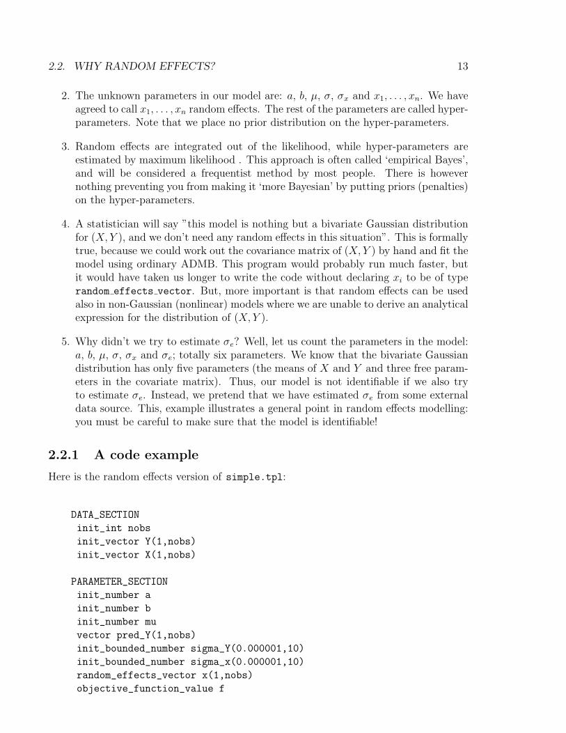
2. The unknown parameters in our model are: a, b, µ, σ, σx and x1, . . . , xn. We haveagreed to call x1, . . . , xn random effects. The rest of the parameters are called hyper-parameters. Note that we place no prior distribution on the hyper-parameters.
3. Random effects are integrated out of the likelihood, while hyper-parameters areestimated by maximum likelihood . This approach is often called ‘empirical Bayes’,and will be considered a frequentist method by most people. There is howevernothing preventing you from making it ‘more Bayesian’ by putting priors (penalties)on the hyper-parameters.
4. A statistician will say ”this model is nothing but a bivariate Gaussian distributionfor (X, Y ), and we don’t need any random effects in this situation”. This is formallytrue, because we could work out the covariance matrix of (X, Y ) by hand and fit themodel using ordinary ADMB. This program would probably run much faster, butit would have taken us longer to write the code without declaring xi to be of typerandom effects vector. But, more important is that random effects can be usedalso in non-Gaussian (nonlinear) models where we are unable to derive an analyticalexpression for the distribution of (X, Y ).
5. Why didn’t we try to estimate σe? Well, let us count the parameters in the model:a, b, µ, σ, σx and σe; totally six parameters. We know that the bivariate Gaussiandistribution has only five parameters (the means of X and Y and three free param-eters in the covariate matrix). Thus, our model is not identifiable if we also tryto estimate σe. Instead, we pretend that we have estimated σe from some externaldata source. This, example illustrates a general point in random effects modelling:you must be careful to make sure that the model is identifiable!
2.2.1 A code example
Here is the random effects version of simple.tpl:
DATA_SECTION
init_int nobs
init_vector Y(1,nobs)
init_vector X(1,nobs)
PARAMETER_SECTION
init_number a
init_number b
init_number mu
vector pred_Y(1,nobs)
init_bounded_number sigma_Y(0.000001,10)
init_bounded_number sigma_x(0.000001,10)
random_effects_vector x(1,nobs)
objective_function_value f
14 CHAPTER 2. THE LANGUAGE AND THE PROGRAM
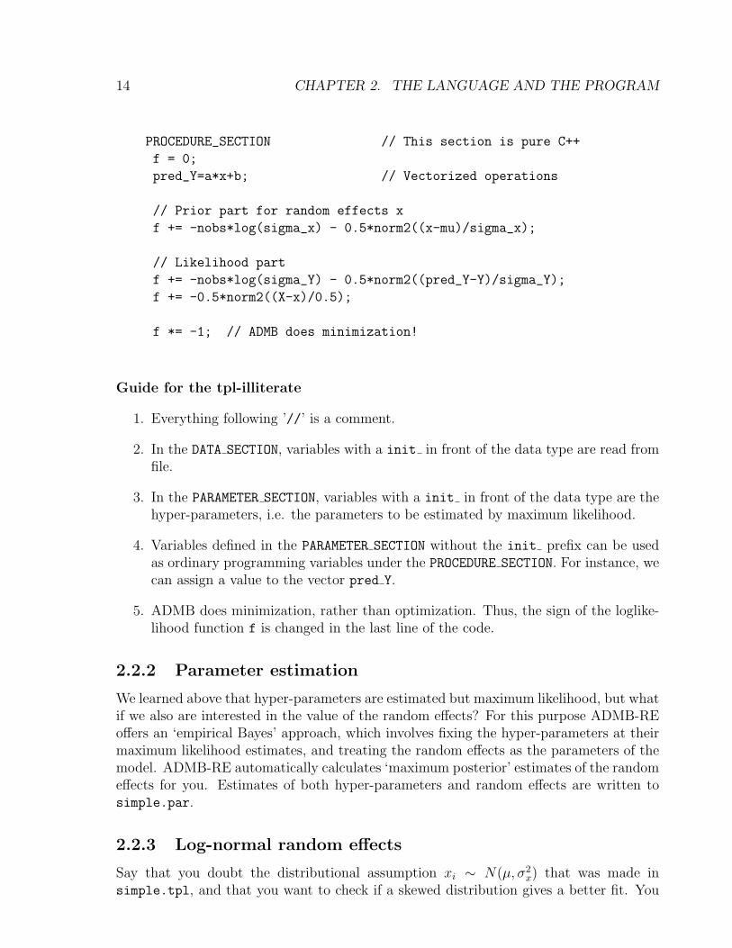
PROCEDURE_SECTION // This section is pure C++
f = 0;
pred_Y=a*x+b; // Vectorized operations
// Prior part for random effects x
f += -nobs*log(sigma_x) - 0.5*norm2((x-mu)/sigma_x);
// Likelihood part
f += -nobs*log(sigma_Y) - 0.5*norm2((pred_Y-Y)/sigma_Y);
f += -0.5*norm2((X-x)/0.5);
f *= -1; // ADMB does minimization!
Guide for the tpl-illiterate
1. Everything following ’//’ is a comment.
2. In the DATA SECTION, variables with a init in front of the data type are read fromfile.
3. In the PARAMETER SECTION, variables with a init in front of the data type are thehyper-parameters, i.e. the parameters to be estimated by maximum likelihood.
4. Variables defined in the PARAMETER SECTION without the init prefix can be usedas ordinary programming variables under the PROCEDURE SECTION. For instance, wecan assign a value to the vector pred Y.
5. ADMB does minimization, rather than optimization. Thus, the sign of the loglike-lihood function f is changed in the last line of the code.
2.2.2 Parameter estimation
We learned above that hyper-parameters are estimated but maximum likelihood, but whatif we also are interested in the value of the random effects? For this purpose ADMB-REoffers an ‘empirical Bayes’ approach, which involves fixing the hyper-parameters at theirmaximum likelihood estimates, and treating the random effects as the parameters of themodel. ADMB-RE automatically calculates ‘maximum posterior’ estimates of the randomeffects for you. Estimates of both hyper-parameters and random effects are written tosimple.par.
2.2.3 Log-normal random effects
Say that you doubt the distributional assumption xi ∼ N(µ, σ2x) that was made in
simple.tpl, and that you want to check if a skewed distribution gives a better fit. You
2.3. RANDOM EFFECTS MODELING 15
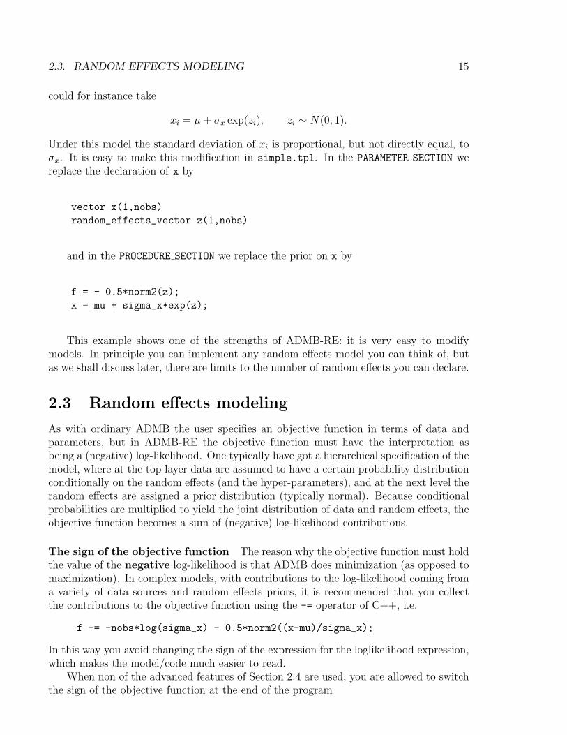
could for instance take
xi = µ + σx exp(zi), zi ∼ N(0, 1).
Under this model the standard deviation of xi is proportional, but not directly equal, toσx. It is easy to make this modification in simple.tpl. In the PARAMETER SECTION wereplace the declaration of x by
vector x(1,nobs)
random_effects_vector z(1,nobs)
and in the PROCEDURE SECTION we replace the prior on x by
f = - 0.5*norm2(z);
x = mu + sigma_x*exp(z);
This example shows one of the strengths of ADMB-RE: it is very easy to modifymodels. In principle you can implement any random effects model you can think of, butas we shall discuss later, there are limits to the number of random effects you can declare.
2.3 Random effects modeling
As with ordinary ADMB the user specifies an objective function in terms of data andparameters, but in ADMB-RE the objective function must have the interpretation asbeing a (negative) log-likelihood. One typically have got a hierarchical specification of themodel, where at the top layer data are assumed to have a certain probability distributionconditionally on the random effects (and the hyper-parameters), and at the next level therandom effects are assigned a prior distribution (typically normal). Because conditionalprobabilities are multiplied to yield the joint distribution of data and random effects, theobjective function becomes a sum of (negative) log-likelihood contributions.
The sign of the objective function The reason why the objective function must holdthe value of the negative log-likelihood is that ADMB does minimization (as opposed tomaximization). In complex models, with contributions to the log-likelihood coming froma variety of data sources and random effects priors, it is recommended that you collectthe contributions to the objective function using the -= operator of C++, i.e.
f -= -nobs*log(sigma_x) - 0.5*norm2((x-mu)/sigma_x);
In this way you avoid changing the sign of the expression for the loglikelihood expression,which makes the model/code much easier to read.
When non of the advanced features of Section 2.4 are used, you are allowed to switchthe sign of the objective function at the end of the program
16 CHAPTER 2. THE LANGUAGE AND THE PROGRAM
f *= -1; // ADMB does minimization!
so that in fact f holds the value of the log-likelihood until the last line of the program.The order in which the different loglikelihood contributions are added to the objective
function does not matter, but make sure that all programming variables have got theirvalue assigned before they enter in a prior or a likelihood expression.
In simple.tpl we declared x1, . . . , xn to be of type random effects vector. Thisstatement tells ADMB that x1, . . . , xn should be treated as random effects (i.e. be thetargets for the Laplace approximation), but it does not say anything about which distribu-tion the random effects should have. In the simple.tpl we assumed that xi ∼ N(µ, σ2
x),and (without saying it explicitly) that the xi’s were statistically independent. We knowthat the corresponding prior contribution to the loglikelihood is
−n log(σx)−1
2σ2x
∑i=1
(xi − µ)2 .
The corresponding ADMB code is
f += -nobs*log(sigma_x) - 0.5*norm2((x-mu)/sigma_x);
Usually, the random effects will have a Gaussian distribution, but technically speakingthere is nothing preventing you from replacing the above line by for instance a log-gammadensity. It can be expected that the Laplace approximation will be less accurate. Achange-of-variable transformation for the random effects may be use to improve the ac-curacy of the Laplace approximation (not discussed in this manual).
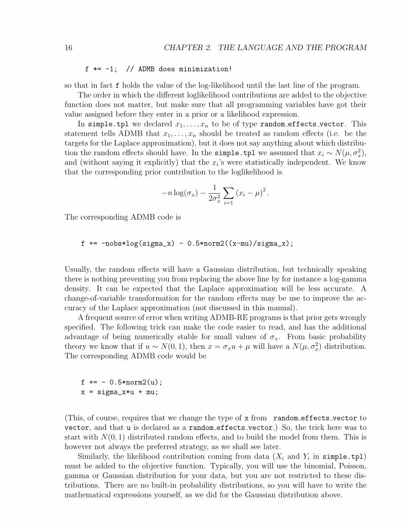
A frequent source of error when writing ADMB-RE programs is that prior gets wronglyspecified. The following trick can make the code easier to read, and has the additionaladvantage of being numerically stable for small values of σx. From basic probabilitytheory we know that if u ∼ N(0, 1), then x = σxu + µ will have a N(µ, σ2
x) distribution.The corresponding ADMB code would be
f += - 0.5*norm2(u);
x = sigma_x*u + mu;
(This, of course, requires that we change the type of x from random effects vector tovector, and that u is declared as a random effects vector.) So, the trick here was tostart with N(0, 1) distributed random effects, and to build the model from them. This ishowever not always the preferred strategy, as we shall see later.
Similarly, the likelihood contribution coming from data (Xi and Yi in simple.tpl)must be added to the objective function. Typically, you will use the binomial, Poisson,gamma or Gaussian distribution for your data, but you are not restricted to these dis-tributions. There are no built-in probability distributions, so you will have to write themathematical expressions yourself, as we did for the Gaussian distribution above.

2.3. RANDOM EFFECTS MODELING 17
2.3.1 Correlated random effects
In some situation you will need correlated random effects, and as part of the problemyou may want to estimate the elements of the covariance matrix. To ensure that thecorrelation matrix C is positive definite, you can parameterize the problem in terms ofthe Cholesky factor L, i.e. C = LL′, where L is a lower diagonal matrix with positivediagonal elements. There are q(q − 1)/2) free parameters (the non-zero elements of L)to be estimated, where q is the dimension of C. Since C is a correlation matrix we mustensure that its diagonal elements are unity. An example with q = 4 is
PARAMETER_SECTION
matrix L(1,4,1,4) // Cholesky factor
init_vector a(1,6) // Free parameters
PROCEDURE_SECTION
int k;
L(1,1) = 1.0;
for(i=2;i<=4;i++)
{
L(i,i) = 1.0;
for(j=1;j<=i-1;j++)
L(i,j) = a(k++);
L(i)(1,i) /= norm(L(i)(1,i)); // Ensures that C(i,i) = 1
}
Given the Cholesky factor L, we can proceed in different directions. One option is touse the same transformation-of-variable technique as above: Start out with a vector u ofindependent N(0, 1) distributed random effects. Then, the vector
x = L*u;
has correlation matrix C = LL′. To scale the variances, we multiply each component ofx by the appropriate standard deviation.
Large structured covariance matrices In some situations, for instance in spatialmodels, q will be large (q = 100, say). Then it is better to use the approach outlined inSection 2.5.3.
2.3.2 Non-Gaussian random effects
It is customary to use normally distributed random effects, but in some situations otherdistributions than the normal are required. The distributions currently available inADMB-RE are: gamma, beta and robust normal distribution (mixture of 2 normal dis-tributions). To use either of these you must
1. Define a random effect u with a N(0, 1) distribution.

18 CHAPTER 2. THE LANGUAGE AND THE PROGRAM
2. Transform u into a new random effect g using one of something deviate functionsdescribed below.
In particular, to obtain av vector g of gamma distributed random effects (probabilitydensity ga−1 exp(−g)/Γ(a)):
PARAMETER_SECTION
init_number a // Shape parameter
vector g(1,n)
random_effects_vector u(1,n,2)
PROCEDURE_SECTION
g -= -0.5*norm2(ui); // N(0,1) likelihood contribution from u’s
for (i=1;i<=n;i++)
g(i) = gamma_deviate(u(i),a);
Full example: http://www.otter-rsch.com/admbre/examples/gamma/gamma.htmlSimilarly, to obtain beta distributed random effects (probability density proportional
to ga−1(1− g)b−1) we use:
PROCEDURE_SECTION
g -= -0.5*norm2(ui); // N(0,1) likelihood contribution from u’s
for (i=1;i<=n;i++)
g(i) = beta_deviate(u(i),a,b);
//g(i)=beta_deviate(u(i),a,b,1.e-7);
The function beta deviate has a fourth parameter (as in the line above that is commentedout) which controls the numerical stability of the function. The use of this parameter iscurrently not documented.
The robust normal distribution has probability density
f(g) = 0.951√2π
e−0.5g2
+ 0.051
c√
2πe−0.5(g/c)2
where c is a “spread” parameter that default is set to c = 3. The corresponding ADMB-RE code is
PROCEDURE_SECTION
g -= - 0.5*norm2(ui); // N(0,1) likelihood contribution from u’s
for (i=1;i<=n;i++)
{
g(i) = robust_normal_mixture_deviate(u(i)); // c = 1.0
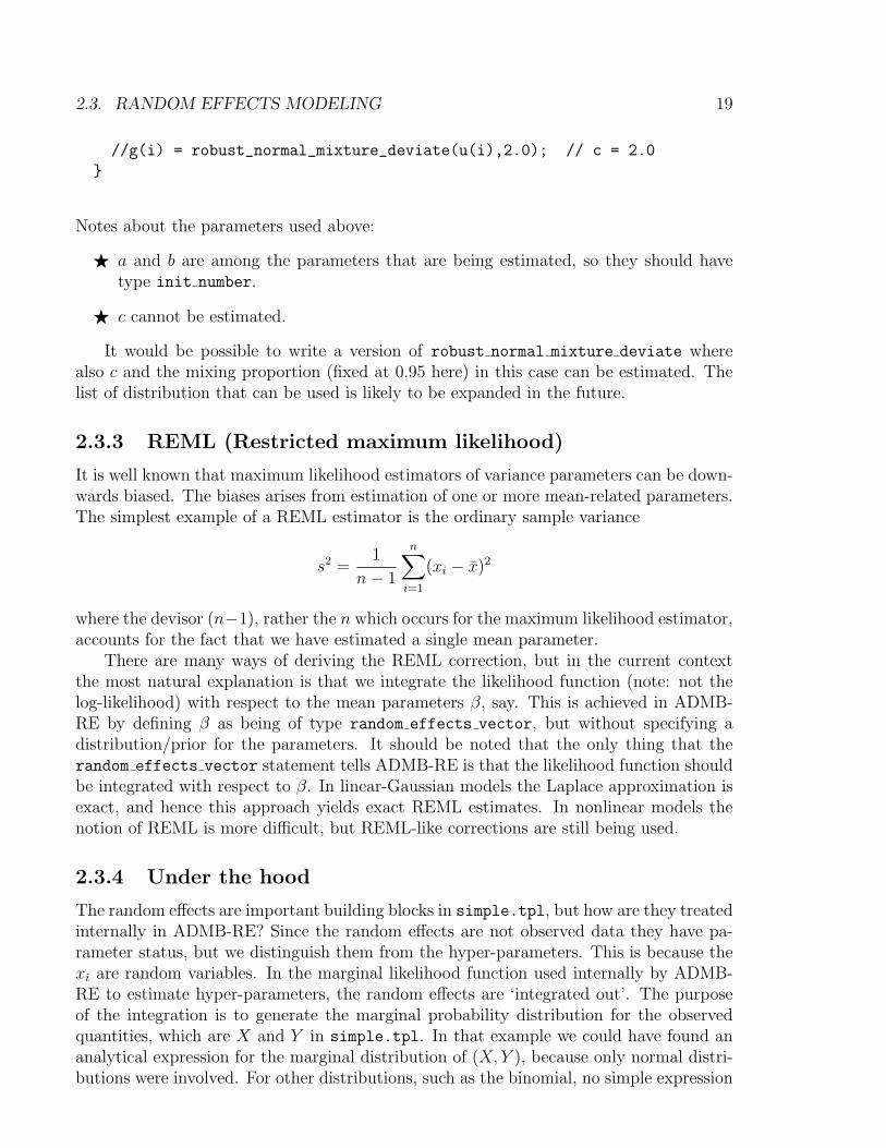
2.3. RANDOM EFFECTS MODELING 19
//g(i) = robust_normal_mixture_deviate(u(i),2.0); // c = 2.0
}
Notes about the parameters used above:
F a and b are among the parameters that are being estimated, so they should havetype init number.
F c cannot be estimated.
It would be possible to write a version of robust normal mixture deviate wherealso c and the mixing proportion (fixed at 0.95 here) in this case can be estimated. Thelist of distribution that can be used is likely to be expanded in the future.
2.3.3 REML (Restricted maximum likelihood)
It is well known that maximum likelihood estimators of variance parameters can be down-wards biased. The biases arises from estimation of one or more mean-related parameters.The simplest example of a REML estimator is the ordinary sample variance
s2 =1
n− 1
n∑i=1
(xi − x̄)2
where the devisor (n−1), rather the n which occurs for the maximum likelihood estimator,accounts for the fact that we have estimated a single mean parameter.
There are many ways of deriving the REML correction, but in the current contextthe most natural explanation is that we integrate the likelihood function (note: not thelog-likelihood) with respect to the mean parameters β, say. This is achieved in ADMB-RE by defining β as being of type random effects vector, but without specifying adistribution/prior for the parameters. It should be noted that the only thing that therandom effects vector statement tells ADMB-RE is that the likelihood function shouldbe integrated with respect to β. In linear-Gaussian models the Laplace approximation isexact, and hence this approach yields exact REML estimates. In nonlinear models thenotion of REML is more difficult, but REML-like corrections are still being used.
2.3.4 Under the hood
The random effects are important building blocks in simple.tpl, but how are they treatedinternally in ADMB-RE? Since the random effects are not observed data they have pa-rameter status, but we distinguish them from the hyper-parameters. This is because thexi are random variables. In the marginal likelihood function used internally by ADMB-RE to estimate hyper-parameters, the random effects are ‘integrated out’. The purposeof the integration is to generate the marginal probability distribution for the observedquantities, which are X and Y in simple.tpl. In that example we could have found ananalytical expression for the marginal distribution of (X, Y ), because only normal distri-butions were involved. For other distributions, such as the binomial, no simple expression

20 CHAPTER 2. THE LANGUAGE AND THE PROGRAM
for the marginal distribution exists, and hence we must rely on ADMB to do the integra-tion. In fact, the core of what ADMB-RE does for you is that it automatically calculatesthe marginal likelihood, at the same time as it estimates the hyper-parameters. The in-tegration technique used by ADMB-RE is the so-called Laplace approximation (Skaug &Fournier 2003).
The algorithm used internally by ADMB-RE to estimate hyper-parameters involvesiterating between the two steps:
1. The ‘penalized likelihood’ step: Maximizing the likelihood with respect to the ran-dom effects, while holding the value of the hyper-parameters fixed.
2. Updating the value of the hyper-parameters, using the estimates of the randomeffects obtained in 1).
The reason for calling the objective function in 1) a penalized likelihood, is that the prioron the random effects acts as a penalty function.
2.3.5 Building a random effects model that works
In all nonlinear parameter estimation problems, there are two possible explanations whenyour program does not produce meaningful results:
1. The underlying mathematical model is not well defined, e.g. it may be over-parameterized.
2. You have implemented the model incorrectly, e.g. you have forgotten a minus signsomewhere.
In an early phase of the code development it may not be clear which of these is causing theproblem. With random effects, the two-step iteration scheme described above makes iteven more difficult to find the error. We therefore advise you always to check the programon simulated data before you apply it to your real dataset. This section gives you a recipefor how to do this.
The first thing you should do after having finished the tpl-file is to check that thepenalized likelihood step is working correctly. In ADMB it is very easy to switch from arandom effects version of the program to a penalized likelihood version. In simple.tpl
we would simply redefine the random effects vector x to be of type init vector. Theparameters would then be a, b, µ, σ, σx and x1, . . . , xn. It is not recommended, or evenpossible, to estimate all of these simultaneously, so you should fix σx (by giving it a phase‘-1’) at some reasonable value. The actual value at which you fix σx is not criticallyimportant, and you could even try a range of σx values. In larger models there will bemore than one parameter that needs to be fixed. We recommend the following scheme:
1. Write a simulation program (in R, S-Plus, Matlab, or some other program) thatgenerates data from the random effects model (using some reasonable values for theparameters) and writes to simple.dat.
2. Fit the penalized likelihood program with σx (or the equivalent parameters) fixedat the value used to simulate data.

2.4. EXPLOITING SEPARABILITY 21
3. Compare the estimated parameters with the parameter values used to simulatedata. In particular, you should plot the estimated x1, . . . , xn against the simulatedrandom effects. The plotted points should centre around a straight line. If they do(to some degree of approximation) you most likely have got a correct formulationof the penalized likelihood.
If your program passes this test, you are ready to test the random effects version of theprogram. You redefine x to be of type random effects vector, free up σx, and applyagain your program to the same simulated dataset. If the program produces meaningfulestimates of the hyper-parameters, you most likely have implemented your model cor-rectly, and you are ready to move on to your real data!
With random effects it often happens that the maximum likelihood estimate of avariance component is zero (σx = 0). Parameters bouncing against the boundaries usuallymakes one feel uncomfortable, but with random effects the interpretation of σx = 0 isclear and unproblematic. All it really means is that data do not support a random effect,and the natural consequence is to remove (or inactivate) x1, . . . , xn, together with thecorresponding prior (and hence σx), from the model.
2.4 Exploiting separability
Above we have shown how to create a model containing latent random variables (randomeffects). This description is sufficient for models with a small number of latent randomvariables, but in order to deal with larger models it is necessary to exploit any specialstructure that the model may have. Such special structures are best described withreference to common classes of latent variable models:
• Nested random effects.
• Time series structure.
• Crossed random effects.
ADMB-RE is able two exploit these structures in two different ways, both of which helpimproving the performance: 1) derivative calculations can be simplifid and 2) the in-ternal matrix computations may be performed with sparse matrix libraries. The key toachieving efficiency is to break up the computation into a series of calls to a one or moreSEPARABLE FUNCTION’s, in such a way that each call only involves a few latent randomvariables.
2.4.1 The first example
A simple example is the one-way variance component model
yij = µ + σuui + εij, i = 1, . . . , q, j = 1, . . . , ni
where ui ∼ N(0, 1) is a random effect and εij ∼ N(0, σ2) is an error term. The straight-forward implementation of this model (shown only in part) is

22 CHAPTER 2. THE LANGUAGE AND THE PROGRAM
PARAMETER_SECTION
random_effects_vector u(1,q)
PROCEDURE_SECTION
for(i=1;i<=q;i++)
{
g -= -0.5*square(u(i));
for(j=1;j<=n(i);j++)
g -= -log(sigma) - 0.5*square((y(i,j)-mu-sigma_u*u(i))/sigma);
}
The efficient implementation of this model is
PROCEDURE_SECTION
for(i=1;i<=q;i++)
g_cluster(i,u(i),mu,sigma,sigma_u);
SEPARABLE_FUNCTION void g_cluster(int i, const dvariable& u,...)
g -= -0.5*square(u);
for(int j=1;j<=n(i);j++)
g -= -log(sigma) - 0.5*square((y(i,j)-mu-sigma_u*u)/sigma);
where ... replaces the rest of the argument list (due to lack of space in this document).It is the function call g cluster(i,u(i),mu,sigma,sigma u) that enables ADMB-
RE to identify the special structure of the model, which in this case is a trivial instanceof nesting. Knowing about the nesting structure enables ADMB-RE to do a series ofunivariate Laplace approximations, rather than a single Laplace approximation in fulldimension q. It should then be possible to fit models where q is in the order of thousands,but this clearly depends on the complexity of the function g cluster.
The following rules apply:
F The argument list in the definition of the SEPARABLE FUNCTION should not brokeninto several lines of text in the tpl-file. This is often tempting as the line typicallygets long, but it results in an error message from tpl2rem.
F Objects defined in the PARAMETER SECTION must be passed as arguments to g cluster.There is one exception: the objective function g is a global object, and does notneed to be as an argument. Temporary variables should be defined locally withinthe SEPARABLE FUNCTION.
F Objects defined in the DATA SECTION should not be passed as arguments to g cluster
(they are also global objects).
The data types that currently can be passed as arguments to a SEPARABLE FUNCTION are:

2.4. EXPLOITING SEPARABILITY 23
int
const dvariable&
const dvar_vector&
with an example being
SEPARABLE_FUNCTION void f(int i, const dvariable& a, const dvar_vector& beta)
The qualifier const is required for the latter two data types, and signalizes to theC++ compiler that the value of the variable is not going to be changed by the func-tion. You may also come across the type const prevariable& which means exactly thesame as const dvariable&.
There are other rules that have to be obeyed:
F No calculations involving variables defined in the PARAMETER SECTION are allowedin the PROCEDURE SECTION. The only use of such variables there is passing them asarguments to SEPARABLE FUNCTION’s.
This rule implies that all the action has to take place inside the SEPARABLE FUNCTION’s.To minimize the number of parameters that have be passed as arguments, the followingprogramming practice is recommended when using SEPARABLE FUNCTION’s:
F The PARAMETER SECTION should contain definitions only of parameters (those vari-ables which type has a init prefix) and random effects, i.e. no temporary program-ming variables.
All temporary variables needed for the computations should be defined locally in theSEPARABLE FUNCTION as shown here:
SEPARABLE_FUNCTION void prior(const dvariable& log_s, const dvariable& u)
dvariable sigma_u = exp(log_s);
g -= -log_s - 0.5*square(u(i)/sigma_u);
2.4.2 Nested models
In the above model there is no hierarchical structure among the latent random variables(the u’s). A more complicated example is provided by the following model:
yijk = σvvi + σuuij + εijk, i = 1, . . . , q, j = 1, . . . ,m, k = 1, . . . , nij,
where the random effects vi and uij are independent N(0, 1) distributed, and εij ∼N(0, σ2) is still the error term. One often say that the u’s are nested within the v’s.For i1 6= i2 we have that yi1jk and yi2jk are statistically independent, so that the likeli-hood factors at the outer nesting level (i). To exploit this we use the SEPARABLE FUNCTION
as follows:
24 CHAPTER 2. THE LANGUAGE AND THE PROGRAM
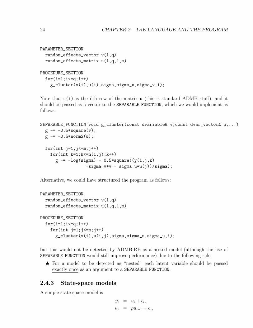
PARAMETER_SECTION
random_effects_vector v(1,q)
random_effects_matrix u(1,q,1,m)
PROCEDURE_SECTION
for(i=1;i<=q;i++)
g_cluster(v(i),u(i),sigma,sigma_u,sigma_v,i);
Note that u(i) is the i’th row of the matrix u (this is standard ADMB stuff), and itshould be passed as a vector to the SEPARABLE FUNCTION, which we would implement asfollows:
SEPARABLE_FUNCTION void g_cluster(const dvariable& v,const dvar_vector& u,...)
g -= -0.5*square(v);
g -= -0.5*norm2(u);
for(int j=1;j<=m;j++)
for(int k=1;k<=n(i,j);k++)
g -= -log(sigma) - 0.5*square((y(i,j,k)
-sigma_v*v - sigma_u*u(j))/sigma);
Alternative, we could have structured the program as follows:
PARAMETER_SECTION
random_effects_vector v(1,q)
random_effects_matrix u(1,q,1,m)
PROCEDURE_SECTION
for(i=1;i<=q;i++)
for(int j=1;j<=m;j++)
g_cluster(v(i),u(i,j),sigma,sigma_u,sigma_u,i);
but this would not be detected by ADMB-RE as a nested model (although the use ofSEPARABLE FUNCTION would still improve performance) due to the following rule:
F For a model to be detected as “nested” each latent variable should be passedexactly once as an argument to a SEPARABLE FUNCTION.
2.4.3 State-space models
A simple state space model is
yi = ui + εi,
ui = ρui−1 + ei,

2.4. EXPLOITING SEPARABILITY 25
where ei ∼ N(0, σ2) is an inovation term. The log-likelihood contribution comming fromthe state vector (u1, . . . , un) is
n∑i=2
log
(1√2πσ
exp
[−(ui − ρui−1)
2
2σ2
]),
where (u1, . . . , un) is the state vector. To make ADMB-RE exploit this special structurewe write a SEPARABLE FUNCTION named g conditional, that implements the individualterms in the above sum. This function would then be invoked as follows
for(i=2;i<=n;i++)
g_conditional(u(i),u(i-1),rho,sigma);
Full example http://www.otter-rsch.com/admbre/examples/polio/polio.html.Above we have looked at a model with a univariate state vector. For multivariate
state vectors, as in
yi = ui + vi + εi,
ui = ρ1ui−1 + ei,
vi = ρ2vi−1 + di,
we would merge the u and v vectors into a single vector (u1, v1, u2, v2, . . . , un, vn), anddefine
random_effects_vector u(1,m)
where m = 2n. The call to the SEPARABLE FUNCTION would now look like
for(i=2;i<=n;i++)
g_conditional(u(2*(i-2)+1),u(2*(i-2)+2),u(2*(i-2)+3),u(2*(i-2)+4),...);
where ... denotes the arguments ρ1, ρ2, σe and σd.
2.4.4 Frequency weighting for multinomial likelihoods
In situations were the response variable only can take on a finite number of differentvalues, it is possibly to reduce the computational burden enormously. As an example,consider a situation where observation yi is binomially distributed with paramters N = 2and pi. Assume that
pi =exp(µ + ui)
1 + exp(µ + ui),
26 CHAPTER 2. THE LANGUAGE AND THE PROGRAM
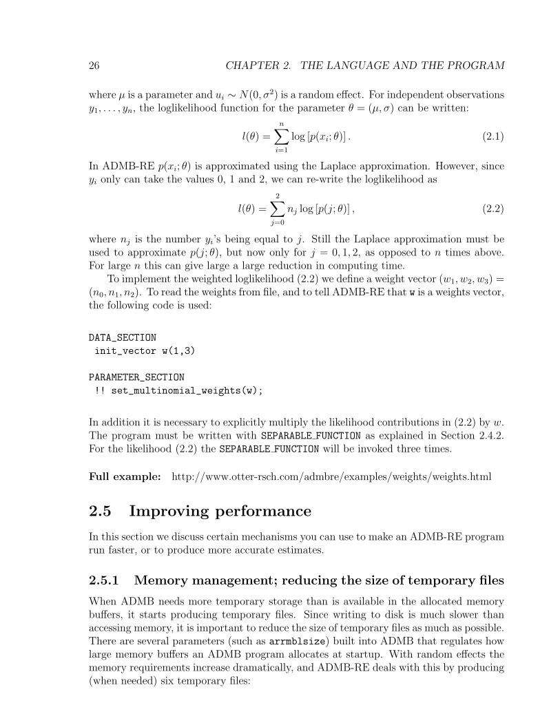
where µ is a parameter and ui ∼ N(0, σ2) is a random effect. For independent observationsy1, . . . , yn, the loglikelihood function for the parameter θ = (µ, σ) can be written:
l(θ) =n∑
i=1
log [p(xi; θ)] . (2.1)
In ADMB-RE p(xi; θ) is approximated using the Laplace approximation. However, sinceyi only can take the values 0, 1 and 2, we can re-write the loglikelihood as
l(θ) =2∑
j=0
nj log [p(j; θ)] , (2.2)
where nj is the number yi’s being equal to j. Still the Laplace approximation must beused to approximate p(j; θ), but now only for j = 0, 1, 2, as opposed to n times above.For large n this can give large a large reduction in computing time.
To implement the weighted loglikelihood (2.2) we define a weight vector (w1, w2, w3) =(n0, n1, n2). To read the weights from file, and to tell ADMB-RE that w is a weights vector,the following code is used:
DATA_SECTION
init_vector w(1,3)
PARAMETER_SECTION
!! set_multinomial_weights(w);
In addition it is necessary to explicitly multiply the likelihood contributions in (2.2) by w.The program must be written with SEPARABLE FUNCTION as explained in Section 2.4.2.For the likelihood (2.2) the SEPARABLE FUNCTION will be invoked three times.
Full example: http://www.otter-rsch.com/admbre/examples/weights/weights.html
2.5 Improving performance
In this section we discuss certain mechanisms you can use to make an ADMB-RE programrun faster, or to produce more accurate estimates.
2.5.1 Memory management; reducing the size of temporary files
When ADMB needs more temporary storage than is available in the allocated memorybuffers, it starts producing temporary files. Since writing to disk is much slower thanaccessing memory, it is important to reduce the size of temporary files as much as possible.There are several parameters (such as arrmblsize) built into ADMB that regulates howlarge memory buffers an ADMB program allocates at startup. With random effects thememory requirements increase dramatically, and ADMB-RE deals with this by producing(when needed) six temporary files:

2.5. IMPROVING PERFORMANCE 27
File name Command line optionf1b2list1 -l1 N
f1b2list12 -l2 N
f1b2list13 -l3 N
nf1b2list1 -nl1 N
nf1b2list12 -nl2 N
nf1b2list13 -nl3 N
The table also shows the command line arguments you can use to manually set the size(determined by N) of the different memory buffers.
When you see any of these files start growing, you should kill your application andrestart it with the appropriate command line options. In addition to the options shownabove there is -ndb N that splits the computations into N chunks. This effectively reducesthe memory requirements by a factor of N , at the cost of a somewhat longer run time.It is necessary that N is a divisor of the total number of random effects in the model, sothat it is possible to split the job into N iqually large parts. The -ndb option can be usedin combination with the -l and -nl options listed above. The following rule-of-thumb forsetting N in -ndb N can be used: if there are totally m random effects in the model, oneshould choose N such that m/N ≈ 50. For most of the models in the example collection(Chapter 3) this choice of N prevents any temporary files of being created.
Consider the model http://otter-rsch.com/admbre/examples/union/union.htmlas an example. This model contains only about 60 random effects, but does rather heavycomputations with these, and as a consequence large temporary files are generated. Thefollowing command line
$ ./union -l1 10000000 -l2 100000000 -l3 10000000 -nl1 10000000
takes away the temporary files but requires 80Mb of memory. The command line
$ ./union -est -ndb 5 -l1 10000000
also runs without temporary files, requires only 20Mb of memory, but runs three timesslower.
Finally, a warning about the use of these command line options. If you allocate toomuch memory your application will crash, and you will (should) get a meaningful errormessage. You should monitor the memory use of your application using “Task Manager”under Windows and the command “top” under Linux, to ensure that you do not exceedthe available memory on your computer.
2.5.2 Limited memory Newton optimization
The penalized likelihood step (Section 2.3.4), that forms a crucial part of the algorithmused by ADMB to estimate hyper-parameters, is by default conducted using a quasi-Newton optimization algorithm. If the number of random effects is large, as it typicallyis for separable models, it may be more efficient to use a ‘limited memory quasi-Newton’optimization algorithm. This is done using the command line argument -ilmn N, whereN is the number of steps to keep. Typically N=5 is a good choice.

28 CHAPTER 2. THE LANGUAGE AND THE PROGRAM
2.5.3 Gaussian priors and quadratic penalties
In most models the prior for the random effect will be Gaussian. In some situations,such as in spatial statistics, all the individual components of the random effects vectorwill be jointly correlated. ADMB contains a special feature (the normal prior keyword)for dealing efficiently with such models. The construct used to declaring a correlatedGaussian prior is
random_effects_vector u(1,n)
normal_prior S(u);
The first of these lines is an ordinary declaration of a random effects vector. The secondline tells ADMB that u has a multivariate Gaussian distribution with zero expectationand covariance matrix S , i.e. the probability density of u is
h(u) = (2π)−1/2 det(S)−1/2 exp
(−1
2u′S−1u
).
Here, S is allowed to depend on the hyper-parameters of the model. The part of thecode where S gets assigned its value must be placed in a SEPARABLE FUNCTION (see http:
//otter-rsch.com/admbre/examples/spatial/spatial.html).
F The log-prior log (h (u)) is automatically subtracted from the objective function. Itis thus necessary that the objective function holds the negative loglikelihood whenusing the normal prior.
F To verify that your model really is partially separable you should try replacing theSEPARABLE FUNCTION keyword with an ordinary FUNCTION. Then verify on a smallsubset of your data that the two versions of the program produce the same results.You should be able to observe that the SEPARABLE FUNCTION-version runs faster.
2.5.4 Importance sampling
The Laplace approximation may be inaccurate in some situations . The quality of theapproximation may then be improved by adding an importance sampling step. This isdone in ADMB-RE by using the command line argument -is N seed, where N is thesample size in the importance sampling and seed (optional) is used to initialize therandom number generator. Increasing N will give better accuracy, at the cost of a longerrun time. As a rule-of-thumb you should start with N=100, and increase N stepwise by afactor of 2 until the parameter estimates stabilize.
By running the model with different seeds you can check the Monte Carlo error inyour estimates, and possibly average across the different runs to decrease the MonteCarlo error. Replaing the -is N seed option with a -isb N seed gives you a “balanced”sample, which in general should reduce the Monte Carlo error.
For large values of N, the option -is N seed will require a lot of memory, and youwill see that huge temporary files are produced during the execution of the program. Theoption -isf 5 will split the calculations relating to importance sampling into 5 (or anynumber you like) batches. In combination with the techniques discussed in Section 2.5.1,this should reduce the storage requirements. An example of a command line is:

2.5. IMPROVING PERFORMANCE 29
lessafre -isb 1000 9811 -isf 20 -cbs 50000000 -gdb 50000000
The -is option can also be used as a diagnostic tool for checking the accuracy of theLaplace approximation. If you add the -pis (print importance sampling) the importancesampling weights will be printed at the end of the optimization process. If these weightsdo not vary much, the Laplace approximation is probably doing well. On the other hand,if a single weight dominates the others by several orders of magnitude, you are in trouble,and it is likely that even -is N with a large value of N is not going to help you out. Insuch situations, reformulating the model, with the aim of making the loglikelihood closerto a quadratic function in the random effects, is the way to go. See also the followingsection.
2.5.5 Gauss-Hermite quadrature
In the situation where the model is separable of type ”block diagonal Hessian” with only asingle random effect in each block (see Section 2.4), Gauss-Hermite quadrature is availableas an option to the Laplace approximation and the -is option (importance sampling). Itis invoked with command line option -gh N where N is the number of quadrature points.
2.5.6 Phases
A very useful feature of ADMB is that it allows the model to be fit in different phases.In the first phase you estimate only a subset of the parameters, with the remainingparameters being fixed at their initial values. In the second phase more parameters areturned on, and so it goes. The phase in which a parameter becomes active is specified inthe declaration of the parameter. By default a parameter has phase 1. A simple examplewould be
PARAMETER_SECTION
init_number a(1)
random_effects_vector b(1,10,2)
where a becomes active in phase 1, while b is a vector of length 10 that becomes active inphase 2. With random effects we have the following rule-of-thumb for the use of phases:
1. Activate the random effects and the corresponding variance parameter in phase 2.
2. Activate the remaining hyper-parameters in phase 1.
When there are more than one random effects vector, it may be advantageous to let thesebecome active in different phases.
During program development it is often useful to be able to completely switch aparameters off. A parameter is inactivated when given phase ‘-1’ as in
PARAMETER_SECTION
init_number c(-1)

30 CHAPTER 2. THE LANGUAGE AND THE PROGRAM
The parameter is still part of the program, and its value will still be read from the pin-file,but it does not take part in the optimization (in any phase).
For further details about phases, please consult the section ‘Carrying out the mini-mization in a number of phases’ in the ADMB manual (not this document).
2.5.7 MCMC
There are two different MCMC methods built into ADMB-RE: -mcmc and -mcmc2. Bothare based on the Metropolis-Hastings algorithm. The former generates a Markov chain onthe hyper-parameters only, while -mcmc2 generates a chain on the joint vector of hyper-parameters and random effects. (Some sort of rejection sampling could be used with -mcmc
to generate values also for the random effects, but this is currently not implemented). Theadvantages of -mcmc are:
• Because there typically is a small number of hyper-parameters, but a large numberof random effects, it is much easier to judge convergence of the chain generatedby -mcmc than that generated by -mcmc2.
• The -mcmc chain mixes faster than the -mcmc2 chain.
The disadvantage of the -mcmc option is that it is slow, because it relies on evaluationof the marginal likelihood by the Laplace approximation. It is recommended to run(separately) both of -mcmc and -mcmc2 to verify that they yield the same posterior forthe hyper-parameters.
2.6 Are all the ADMB-functions in ADMB-RE?
You will find that not all the functionality of ordinary ADMB has yet been implementedin ADMB-RE. Functions are being added all the time.
Appendix A
Command line options
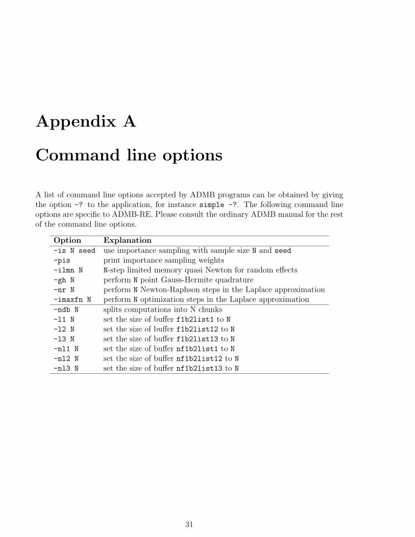
A list of command line options accepted by ADMB programs can be obtained by givingthe option -? to the application, for instance simple -?. The following command lineoptions are specific to ADMB-RE. Please consult the ordinary ADMB manual for the restof the command line options.
Option Explanation-is N seed use importance sampling with sample size N and seed
-pis print importance sampling weights-ilmn N N-step limited memory quasi Newton for random effects-gh N perform N point Gauss-Hermite quadrature-nr N perform N Newton-Raphson steps in the Laplace approximation-imaxfn N perform N optimization steps in the Laplace approximation-ndb N splits computations into N chunks-l1 N set the size of buffer f1b2list1 to N
-l2 N set the size of buffer f1b2list12 to N
-l3 N set the size of buffer f1b2list13 to N
-nl1 N set the size of buffer nf1b2list1 to N
-nl2 N set the size of buffer nf1b2list12 to N
-nl3 N set the size of buffer nf1b2list13 to N
31

32 APPENDIX A. COMMAND LINE OPTIONS

Appendix B
Interfacing ADMB with R
R is a popular freely available software package for statistical analysis. It is convenientto be able to call ADMB programs from R. This appendix explains how to:
• Write data to the .dat and .pin files.
• Call an exe-file produced with ADMB (via the system() function in R).
• Read back the .par and .std files.
It is also possible to compile an ADMB program into an dll that can be linked with R,as described in the chapter “Creating Dynamic Link Libraries with AD Model Builder”of the ADMB manual.
Consider the simple linear regression (y against x). We first generate data in R
> y = rnorm(3)
> x = rnorm(3)
> dat_write("simple",list(n=length(y),y=y,x=x))
which produces the file simple.dat:
# "simple.dat" produced by dat_write() from ADMButils; Wed ...
# n
3
# y
0.4157458 0.07686372 -0.709638
# x
-1.662676 1.193920 -0.08753698
33
34 APPENDIX B. INTERFACING ADMB WITH R
Currently, dat write() handles vector and matrix arguments, but not 3-dimensionalarrays. Similarly, pin write() writes initial values for the parameters to simple.pin.
To invoke simple.exe (assumed to exists in the directory where R is running) wegive the command:
> system("simple",T)
We then read back the results using either of the commands
> L1 = par_read("simple")
> L2 = std_read("simple")
which both return list objects (L1 and L2).

Bibliography
Eilers, P. & Marx, B. (1996), ‘Flexible smoothing with b-splines and penalties’, StatisticalScience 89, 89–121.
Harvey, A., Ruiz, E. & Shephard, N. (1994), ‘Multivariate stochastic variance models’,Review of Economic Studies 61, 247–264.
Hastie, T. & Tibshirani, R. (1990), Generalized Additive Models, Vol. 43 of Monographson Statistics and Applied Probability, Chapman & Hall, London.
Kuk, A. Y. C. & Cheng, Y. W. (1999), ‘Pointwise and functional approximations in MonteCarlo maximum likelihood estimation’, Statistics and Computing 9, 91–99.
Lin, X. & Zhang, D. (1999), ‘Inference in generalized additive mixed models by usingsmoothing splines’, J. Roy. Statist. Soc. Ser. B 61(2), 381–400.
Pinheiro, J. C. & Bates, D. M. (2000), Mixed-Effects Models in S and S-PLUS, Statisticsand Computing, Springer.
Ruppert, D., Wand, M. & Carroll, R. (2003), Semiparametric Regression, CambridgeUniversity Press.
Skaug, H. & Fournier, D. (2003), Evaluating the Laplace approximation by automaticdifferentiation in nonlinear hierarchical models, Unpublished manuscript: Inst. ofMarine Research, Box 1870 Nordnes, 5817 Bergen, Norway.
Zeger, S. L. (1988), ‘A regression-model for time-series of counts’, Biometrika 75, 621–629.
35

Index
command line optionsADMB-RE specific, 31
Gauss-Hermite quadrature, 29
hyper-parameter, 13
importance sampling, 28
limited memory quasi-Newton, 27linear predictor, 11
mcmc, 30
penalized likelihood, 20phases, 29prior distributions
Gaussian priors, 28
random effects, 12correlated, 17Laplace approximation, 20random effects matrix, 12random effects vector, 12
temporary filesf1b2list1, 26reducing the size, 26
tpl-filecompiling, 10, 11writing, 9
36