Random-Number Generation

Discrete-Event System Simulation

2

Purpose & Overview

Discuss the generation of random numbers.

Introduce the subsequent testing for randomness: Frequency test Autocorrelation test.

3

Properties of Random Numbers

Two important statistical properties: Uniformity Independence.

Random Number, Ri, must be independently drawn from a uniform distribution with pdf:

Figure: pdf for random numbers

otherwise ,0

10 ,1)(

xxf

2

1

2)(

1

0

21

0

xxdxRE

4

Generation of Pseudo-Random Numbers

“Pseudo”, because generating numbers using a known method removes the potential for true randomness.

Goal: To produce a sequence of numbers in [0,1] that simulates, or imitates, the ideal properties of random numbers (RN).

Important considerations in RN routines: Fast Portable to different computers Have sufficiently long cycle Closely approximate the ideal statistical properties of uniformity

and independence.

5

Techniques for Generating Random #s

Linear Congruential Method (LCM). Combined Linear Congruential Generators (CLCG). Random-Number Streams.

6

Linear Congruential Method

To produce a sequence of integers, X1, X2, … between 0 and m-1 by following a recursive relationship:

The selection of the values for a, c, m, and X0 drastically affects the statistical properties and the cycle length.

The random integers are being generated [0,m-1], and to convert the integers to random numbers:

,...2,1,0 , mod )(1 imcaXX ii

The multiplier

The increment

The modulus

,...2,1 , im

XR i

i

7

Example 7.1

Use X0 = 27, a = 17, c = 43, and m = 100.

The Xi and Ri values are:

X1 = (17*27+43) mod 100 = 502 mod 100 = 2, R1 = 0.02;

X2 = (17*2+43) mod 100 = 77, R2 = 0.77;

X3 = (17*77+43) mod 100 = 52, R3 = 0.52;

…

8

Example 7.2

Look at the Excel worksheet

9

Characteristics of a Good Generator

Maximum Density Such that the values assumed by Ri, i = 1,2,…, leave no large

gaps on [0,1] Solution: a very large integer for modulus m

Maximum Period To achieve maximum density and avoid cycling. Achieve by: proper choice of a, c, m, and X0.

Three rules are given in the text on page 255

Uniformity Apply tests Independence Apply tests

10

Tests for Random Numbers

Two categories: Testing for uniformity:

H0: Ri ~ U[0,1]

H1: Ri ~ U[0,1] Failure to reject the null hypothesis, H0, means that evidence of

non-uniformity has not been detected. Testing for independence:

H0: Ri ~ independently

H1: Ri ~ independently Failure to reject the null hypothesis, H0, means that evidence of

dependence has not been detected.

Level of significance the probability of rejecting H0 when it

is true: = P(reject H0|H0 is true)

/

/

11

Tests

Test of uniformity Kolmogorov-Smirnov test Chi-square test

Test of independence : Autocorrelation test Runs Tests

Runs up and runs down test

Runs above and below the mean

Lenght of runs test Gap test Poker test

12

Kolmogorov-Smirnov Test

Compares the continuous cdf, F(x), of the uniform distribution with the empirical cdf, SN(x), of the N sample observations. We know: If the sample from the RN generator is R1, R2, …, RN, then the

empirical cdf, SN(x) is:

Based on the statistic: D = max| F(x) - SN(x)| Sampling distribution of D is known (a function of N, tabulated in

Table A.8.)

10 ,)( xxxF

N

xRRRxS n

N

are which ,...,, ofnumber )( 21

13

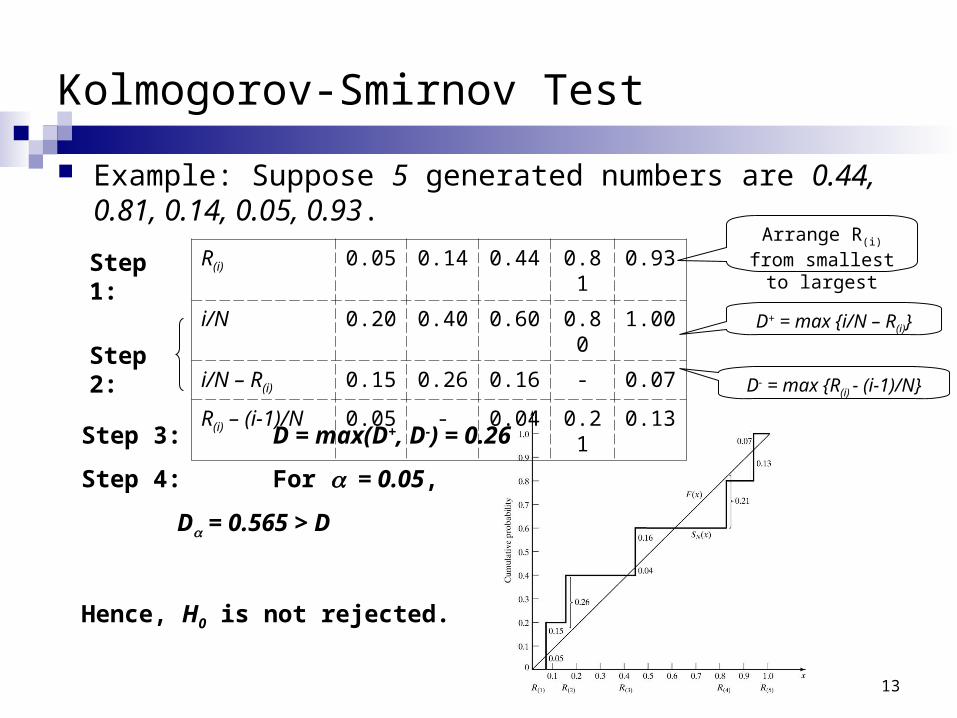
Kolmogorov-Smirnov Test

Example: Suppose 5 generated numbers are 0.44, 0.81, 0.14, 0.05, 0.93.

Step 1:

Step 2:

Step 3: D = max(D+, D-) = 0.26

Step 4: For = 0.05,

D = 0.565 > D

Hence, H0 is not rejected.

Arrange R(i) from smallest to largest

D+ = max {i/N – R(i)}

D- = max {R(i) - (i-1)/N}

R(i) 0.05 0.14 0.44 0.81 0.93

i/N 0.20 0.40 0.60 0.80 1.00

i/N – R(i) 0.15 0.26 0.16 - 0.07

R(i) – (i-1)/N 0.05 - 0.04 0.21 0.13

14

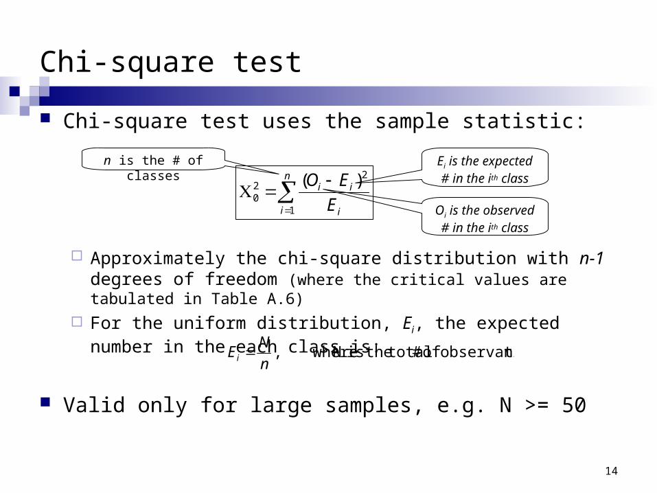
Chi-square test

Chi-square test uses the sample statistic:

Approximately the chi-square distribution with n-1 degrees of freedom (where the critical values are tabulated in Table A.6)

For the uniform distribution, Ei, the expected number in the each class is:

Valid only for large samples, e.g. N >= 50

n

i i

ii

E

EO

1

220

)(

nobservatio of # total theis N where,n

NEi

n is the # of classes

Oi is the observed # in the ith class

Ei is the expected # in the ith class

15

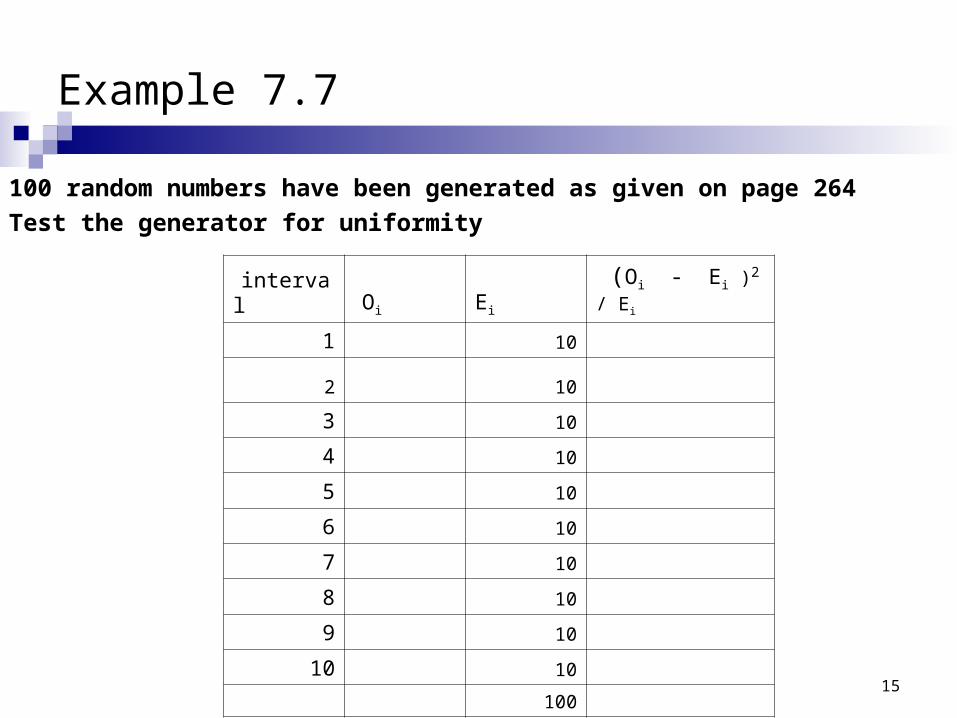
Example 7.7

100 random numbers have been generated as given on page 264

Test the generator for uniformity

 interval  Oi Ei  (Oi - Ei )2 / Ei

 1    10  

 2  10

 3    10  

 4    10  

 5    10  

 6    10  

 7    10  

 8    10  

 9    10  

 10    10  

     100  

16

Tests for Autocorrelation

Testing the autocorrelation between every m numbers (m is a.k.a. the lag), starting with the ith number The autocorrelation im between numbers: Ri, Ri+m, Ri+2m, Ri+(M+1)m

M is the largest integer such that

Hypothesis:

If the values are uncorrelated: For large values of M, the distribution of the estimator of im,

denoted is approximately normal.

N)m (Mi 1

im̂

dependent are numbers if

tindependen are numbers if

,0 :

,0 :

1

0

im

im

H

H

17

Tests for Autocorrelation

Test statistics is:

Z0 is distributed normally with mean = 0 and variance = 1, and:

If im > 0, the subsequence has positive autocorrelation High random numbers tend to be followed by high ones, and vice versa.

If im < 0, the subsequence has negative autocorrelation Low random numbers tend to be followed by high ones, and vice versa.

im

imZ

ˆ

0 ˆ

ˆ

)(M

Mσ

.RRM

ρ

imρ

M

k)m(kikmiim

112

713ˆ

2501

1ˆ

01

18

Example 7.8

Data from Page 265: test for autocorrelation

0.12 0.01 0.23 0.28 0.89 0.31 0.64 0.28 0.83 0.93

0.99 0.15 0.33 0.35 0.91 0.41 0.60 0.27 0.75 0.88

0.68 0.49 0.05 0.43 0.95 0.58 0.19 0.36 0.69 0.87

19

Example 7.8

Test whether the 3rd, 8th, 13th, and so on, for the following output on Page 265. Hence, = 0.05, i = 3, m = 5, N = 30, and M = 4

From Table A.3, z0.025 = 1.96. Hence, the hypothesis is not rejected.

516.11280.0

1945.0

128.01412

7)4(13ˆ

1945.0

250)36.0)(05.0()05.0)(28.0(

)27.0)(33.0()33.0)(28.0()28.0)(23.0(

14

1ˆ

0

35

35

Z

)(σ

.ρ

ρ

20

Summary

In this chapter, we described: Generation of random numbers Testing of generators for uniformity Testing of generators for independence

Caution: Even with generators that have been used for years, some of

which still in used, are found to be inadequate. Also, even if generated numbers pass all the tests, some

underlying pattern might have gone undetected.