1/28

Random Projection Estimation of Discrete-ChoiceModels with Large Choice Sets

Khai X. Chiong Matthew Shum

USC Caltech

September 2016Machine Learning: What’s in it for Economics?

Becker-Friedman Institute, Univ. of Chicago

2/28

Motivation

Use machine learning ideas in discrete choice models

Workhorse model of demand in economics and marketing.

For applications in economics and marketing: hi-dim dataI E-markets/platforms: Amazon, eBay, Google, Uber, Facebook, etc.

I Large databases from traditional retailers (supermarket data)

Many recent applications of these models face problem thatconsumers’ choice sets are huge:

I Where do Manhattan taxicab drivers wait for fares? (Buchholz 2016)

I Legislators’ choice of language (Gentzkow, Shapiro, Taddy 2016)

I Restaurant choices in NYC (Davis, Dingel, Monras, Morales 2016)

I Choice among bundles of products (eg. Fox and Bajari 2013)

3/28

Specifically:

This paper: address dimension-reduction of large choice setI (not large number of characteristics)1

New application of random projection – tool from machine learningliterature – to reduce dimensionality of choice set.

I One of first uses in econometric modeling2

I Use machine learning techniques in nonlinear econometric setting

Semiparametric: Use convex-analytic properties of discrete-choicemodel (cyclic monotonicity) to derive inequalities for estimation3

1Chernozhukov, Hansen, Spindler 2015; Gillen, Montero, Moon, Shum 20152Ng (2016)3Shi, Shum, Song 2015; Chiong, Galichon, Shum 2016; Melo, Pogorelskiy, Shum

2015

4/28

Multinomial choice with large choice set

Consider discrete choice model. The choice set is j ∈ {0, 1, 2, . . . , d}with d being very large.

Random utility (McFadden) model: choosing product j yields utility

Uj︸︷︷︸utility index

+ εj︸︷︷︸utility shock

with Uj = X ′j β

Xj (dim p × 1) denotes product characteristics (such as prices) and εjis utility shock (random across consumers).

Highest utility option is chosen:

choose j ⇔ Uj + εj ≥ Uj ′ + εj ′ , j′ 6= j

β (dim p × 1) are parameters of interest.

5/28

Discrete-choice model: assumptions and notation

Notation:I ~ε = (ε1, . . . , εd)′, ~U = (U1, . . . ,Ud)′, X ≡ (~X1, · · · , ~Xd)′

I Market share (choice probability): for a given utility vector ~U

sj( ~U) ≡ Pr(Uj + εj ≥ Uj′ + εj′ , j′ 6= j)

Aggregate data: we observe data {~sm,Xm}Mm=1 across markets m

Assumptions:I Utility shocks are independent of regressors: ~ε ⊥ X. No endogeneity.

I Distribution of ~ε is unspecified: semiparametric. Don’t restrictcorrelation patterns among εj , εj′ (may not be IIA).

I Normalize utility from j = 0 to zero.

6/28

Convex analysis and discrete choice

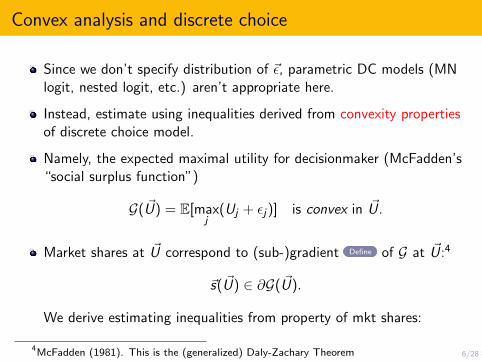
Since we don’t specify distribution of ~ε, parametric DC models (MNlogit, nested logit, etc.) aren’t appropriate here.

Instead, estimate using inequalities derived from convexity propertiesof discrete choice model.

Namely, the expected maximal utility for decisionmaker (McFadden’s“social surplus function”)

G( ~U) = E[maxj

(Uj + εj)] is convex in ~U.

Market shares at ~U correspond to (sub-)gradient Define of G at ~U:4

~s( ~U) ∈ ∂G( ~U).

We derive estimating inequalities from property of mkt shares:

4McFadden (1981). This is the (generalized) Daly-Zachary Theorem

7/28

Estimating inequalities: Cyclic monotonicity

Recall: (sub)-gradient of G( ~U) consists of mkt shares ~s( ~U).

The (sub-)gradient of a (multivariate) convex function is cyclicmonotone: for any cycle of markets m = 1, 2, ..., L, L + 1 = 1

L∑m=1

( ~Um+1 − ~Um) · ~sm ≤ 0 or∑m

(Xm+1 − Xm)′β · ~sm ≤ 0.

Inequalities do not involve ε’s: estimate β semiparametrically.5

These inequalities valid even when some market shares=0I Empirically relevant (store-level scanner data)6

I Consideration sets, rational inattention7

5Shi, Shum, and Song (2015); Melo, Pogorelskiy, Shum (2015)6Gandhi, Lu, Shi (2013). We allow ε to have finite support.7Matejka, McKay 2015

8/28

Introducing random projection

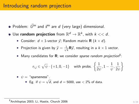
Problem: ~Um and ~sm are d (very large) dimensional.

Use random projection from Rd → Rk , with k << d .

I Consider: d × 1-vector ~y ; Random matrix R (k × d).

I Projection is given by y = 1√k

R~y , resulting in a k × 1 vector.

I Many candidates for R; we consider sparse random projection8:

ri,j ∈√ψ · {+1, 0,−1} with probs.

{1

2ψ, 1− 1

ψ,

1

2ψ

}I ψ = “sparseness”.

F Eg. if ψ =√d , and d = 5000, use < 2% of data.

8Archiloptas 2003; Li, Hastie, Church 2006

9/28

Properties of Random projection

RP replaces high-dim vector ~y with random low-dim vector y withsame length (on average): given ~y , we have:

E[‖y‖2] = E[‖R~y‖2] = ‖~y‖2.

Variance V (y) = O(1/k)

Use of random projection justified by the Johnson-Lindenstrausstheorem:

10/28

Johnson-Lindenstrauss Theorem

Consider projecting d-dim vectors {~w} down to k-dim vectors {w};

There exists an Rd → Rk mapping which preserves Euclidean distanceamong points; ie. for all m1,m2 ∈ {1, 2, . . . ,M} we have, for 0 < δ < 1/2and k = O(log(M)/δ2)

(1− δ)‖~wm1 − ~wm2‖2 ≤ ‖wm1 − wm2‖2 ≤ (1 + δ)‖~wm1 − ~wm2‖2.

The distance between the lower-dim vectors (wm1 , wm2) lies withinδ-neighborhood of distance btw high-dim vectors (~wm1 , ~wm2).

Proof is probabilistic: shows random projection achieves these boundsw/ positive prob.

11/28

The RP Estimator

Observed dataset: D ≡ {~sm,Xm}Mm=1

Projected dataset: Dk ={sm = R~sm, Xm = (R~Xm

1 , . . . ,R~Xmp )}M

m=1.

(Project Xm column-by-column.)

Projected CM inequalities: for all cycles in m ∈ {1, 2, . . . ,M}∑m

(Um+1 − Um) · sm =∑m

(Xm+1 − Xm)′β · sm ≤ 0

The RP Estimator β minimizes the criterion function:

Q(β, D) =∑

all cycles;L≥2

[L∑

m=1

(Xm+1 − Xm)′β · sm

)]2

+

Convex in β (convenient for optimization); may have multiple optima

12/28

Properties of RP estimator

Why does random projection work for our model?

Exploit alternative representation of CM inequalities in terms ofEuclidean distance between vectors:9∑

m

(‖Um − sm‖2 − ‖Um − sm−1‖2

)≤ 0

By JL Theorem, RP preserves Euclidean distances betweencorresponding vectors in D and D.

If CM inequalities satisfied in original dataset D should also be(approximately) satisfied in D.

9Villani 2003

13/28

Properties of RP estimator (cont’d)

RP estimator β is random due to1 randomness in R

2 randomness in market shares smj = 1Nm

∑i 1(yi,j = 1)

For now, focus just on #1: highlight effect of RPI (Assume market shares deterministic; not faroff)

Inference: open questionsI We show uniform convergence of Q(β, D) to Q(β,D) as k grows.

Building block for showing consistency of β

I For inference: little guidance from machine learning literature

I In practice, assess performance of RP estimator across independentRP’s

Monte Carlo ; Two applications 1.Scanner data 2.Mobile advertising

14/28

Monte Carlo Simulations

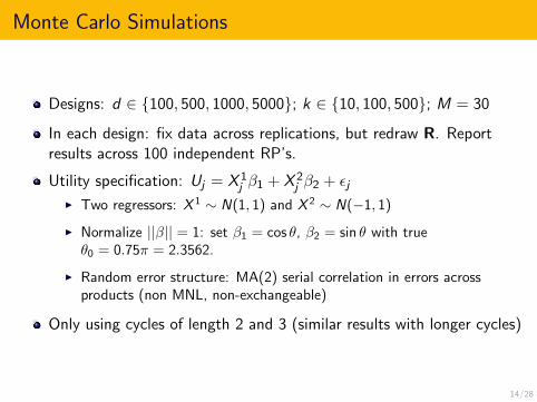
Designs: d ∈ {100, 500, 1000, 5000}; k ∈ {10, 100, 500}; M = 30

In each design: fix data across replications, but redraw R. Reportresults across 100 independent RP’s.

Utility specification: Uj = X 1j β1 + X 2

j β2 + εjI Two regressors: X 1 ∼ N(1, 1) and X 2 ∼ N(−1, 1)

I Normalize ||β|| = 1: set β1 = cos θ, β2 = sin θ with trueθ0 = 0.75π = 2.3562.

I Random error structure: MA(2) serial correlation in errors acrossproducts (non MNL, non-exchangeable)

Only using cycles of length 2 and 3 (similar results with longer cycles)

15/28

Monte Carlo results

Results are robust to different DGP’s for RPI ψ = 1⇒ Dense random projection matrix.

I ψ =√d ⇒ Sparse random projection matrix.

In most cases, optimizing Q(β, D) yields a unique minimum.

On average, estimates close to the true value, but there is dispersionacross RP’s.

16/28

Monte Carlo results: Sparse random projection matrix

Table: Random projection estimator with sparse random projections, ψ =√d

Design mean LB (s.d.) mean UB (s.d.)

d = 100, k = 10 2.3073 (0.2785)d = 500, k = 100 2.2545 (0.2457) 2.3473 (0.2415)d = 1000, k = 100 2.3332 (0.2530) 2.3398 (0.2574)d = 5000, k = 100 2.3671 (0.3144)d = 5000, k = 500 2.3228 (0.3353) 2.5335 (0.3119)

Replicated 100 times using independently realized sparse random projection matrices.

The true value of θ is 2.3562.

17/28

Application I: Store and brand choice in scanner data

Soft drink sales of Dominick’s supermarkets (Rip) in Chicago

Consumers choose both the type of soft drink and store of purchase.

Leverage virtue of semiparametric approach.I Typically store/brand choice modelled as tiered discrete-choice model

(i.e. nested logit).

I Our approach: no need to specify tiering structure. Do consumerschoose stores first and then brands, or vice versa?10

M = 15 “markets” (two-week periods Oct96 - Apr97).

Choose among 11 supermarkets (premium-tier and medium-tier).

A choice is store/UPC combination: d = 3060 available choices.

Reduce to k = 300 using random projection. Results from 100independent RP’s

10Hausman and McFadden (1984)

18/28

Summary Statistics

Definition Summary statistics

sjtFraction of units of store-upc j sold dur-ing market (period) t

Mean: 60.82, s.d: 188.37

pricejtAverage price of the store-upc j duringperiod t

Mean: $2.09, s.d: $1.77

bonusjt

Fraction of weeks in period t for whichstore-upc j was on promotion (eg. “buy-one-get-one-half-off”)

Mean: 0.27, s.d: 0.58

holidaytDummy variable for 11/14/96 to12/25/96 (Thanksgiving, Christmas)

medium tierj Medium, non-premium stores.a 2 out of 11 stores

d Number of store-upc 3059

k Dimension of RP 300

Number of observations is 45885 = 3059 upcs × 15 markets (2-week periods).

19/28

Empirical results

Criterion function always uniquely minimized (but estimate does varyacross different random projections)

Purchase incidence decreasing in price, increasing for bonus, holiday

Price coefficient negativeI and lower on discounted items (bonus): more price sensitive towards

discounted items

I and lower during holiday season: more price sensitive during holidays

No effect of store variables (mediumtier)

(Additional application: 2.Mobile advertising )

20/28

Store/brand choice model estimates

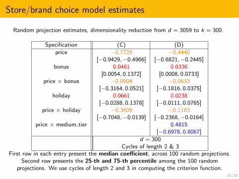
Random projection estimates, dimensionality reduction from d = 3059 to k = 300.

Specification (C) (D)

price −0.7729 −0.4440[−0.9429,−0.4966] [−0.6821,−0.2445]

bonus 0.0461 0.0336[0.0054, 0.1372] [0.0008, 0.0733]

price × bonus −0.0904 −0.0633[−0.3164, 0.0521] [−0.1816, 0.0375]

holiday 0.0661 0.0238[−0.0288, 0.1378] [−0.0111, 0.0765]

price × holiday −0.3609 −0.1183[−0.7048,−0.0139] [−0.2368,−0.0164]

price × medium tier 0.4815[−0.6978, 0.8067]

d = 300Cycles of length 2 & 3

First row in each entry present the median coefficient, across 100 random projections.Second row presents the 25-th and 75-th percentile among the 100 random

projections. We use cycles of length 2 and 3 in computing the criterion function.

21/28

Remarks

For RP estimation, all that is needed is projected dataset D. Neverneed original dataset. Beneficial if privacy is a concern.

Other approaches to large choice sets1 Multinomial logit with “sampled” choice sets.11

2 Maximum score semiparametric approach.12 Use only subset ofinequalities implied by DC model.

F Estimation based on rank-order property (pairwise comparisons amongoptions)

F In binary choice case: CM and ROP coincide.

F For multinomial choice: CM and ROP assumptions non-nested andnon-comparable. Details

3 Moment inequalities.13 Omnibus method

11McFadden (1978); Ben-Akiva, McFadden, Train (1987)12Fox (2007); Fox and Bajari (2013)13Pakes, Porter, Ho, Ishii (2015)

22/28

Conclusions

Multinomial choice problem with huge choice sets

New application of machine learning tool (random projection) fordimension reduction in these models.

Derive semiparametric estimator from cyclic monotonicity inequalities.

Procedure shows promise in simulations and in real-data application.

Random projection may be fruitfully applied in other econometricsettings

Thank you!

23/28

Convex analysis: subgradient/subdifferential/subderivative

Generalization of derivative/gradient for nondifferentiable functions

The subgradient of G at p are vectors u s.t.

G(p) + u · (p′ − p) ≤ G(p′), for all p′ ∈ domG.

Dual relationship between u and p:I ∂G(p) = argmaxu∈R|Y|{p · u − G∗(u)},

where G∗(u) = maxp∈∆|Y|{u · p − G(p)}. (Lemma)

Back

24/28

Remark: Other approaches to large choice sets

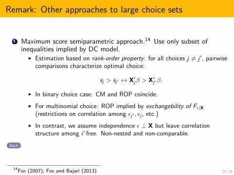
1 Maximum score semiparametric approach.14 Use only subset ofinequalities implied by DC model.

I Estimation based on rank-order property: for all choices j 6= j ′, pairwisecomparisons characterize optimal choice:

sj > sj′ ↔ X′jβ > X′j′β.

I In binary choice case: CM and ROP coincide.

I For multinomial choice: ROP implied by exchangebility of Fε|X(restrictions on correlation among εj′ , εj , etc.)

I In contrast, we assume independence ε ⊥ X but leave correlationstructure among ~ε free. Non-nested and non-comparable.

Back

14Fox (2007); Fox and Bajari (2013)

25/28

Application II: Choosing advertisers in mobile app marketsBack

Model matching in online app market (joint with Richard Chen)

Sellers: publishers sell “impressions” (users of online apps)

Buyers: advertisers who vie to show mobile ad to user. Advertisersbid “cost-per-install” (CPI); only pay when user installs app.

Data from major mobile advertising intermediary: chooses theoptimal ads from one side to show to users on the other side.

Intermediary wants to constantly evaluate whether optimality isachieved. Optimality means choosing advertisers bringing highexpected revenue. Are these advertisers being chosen?

However, difficult to do under CPI mechanism.I CPI payment may benefit advertisers (offering them “free exposure”)

but hurts publishers15

15Hu, Shin, Tang 2016

26/28

Application II: Data Back

Data from a major mobile app advertising intermediary

Estimate model of probability that an advertiser gets chosen inUS-iOS market.

>7700 advertisers. Reduce to 1000.

Advertiser covariates:I Lagged revenue (measure of expected revenue)

I Lagged conversion probability (whether ad viewers install app)

I Genre: gambling

I Self-produced ad

I Whether app is available in Chinese language

27/28

Application II: Results Back

Specification (A) (B) (C) (D)

Revenues 0.823 (0.147) 0.521 (0.072) 0.663 (0.263) 0.657 (0.152)[0.722, 0.937] [0.494, 0.563] [0.711, 0.720] [0.625, 0.748]

ConvProb 0.069 (0.547) 0.037 (0.183) 0.006 (0.035) 0.025 (0.188)[-0.445,0.577] [-0.076,0.161] [-0.013,0.033] [-0.112,0.168]

Rev × Gamble -0.809 (0.187) -0.200 (0.098) -0.192 (0.429)[-0.856,-0.813] [-0.232,-0.185] [-0.500,0.029]

Rev × Client -0.604 (0.278)[-0.673,-0.652]

Rev × Chinese -0.489 (0.228)[-0.649,-0.409]

Dimension reduction: k = 1000Sparsity: s = 3

Cycles of length 2 and 3

Table: Random projection estimates, d = 7660, k = 1000.

First row in each entry present the mean (std dev) coefficient, across 100 randomprojections. Second row presents the 25-th and 75-th percentile among the 100 random

projections. We use cycles of length 2 and 3 in computing the criterion function.

28/28

Application II results and discussion Back

Robust results: expected revenues has strong positive effect, butconversion probability has basically zero effect. Once we control forrevenues, it appears that conversion probability has no impact.

Gamble, client and Chinese all mitigate the effect of revenues.Revenues appear less important for an advertiser when it is a gamblingapp, the creative is self-produced, or if app is available in Chinese.

Are “right” advertisers being chosen?I Yes, to some extent: advertisers offering higher expected revenue are

chosen with higher probability.

I Partially reversed for gambling apps, self-produced ads– sub-optimal?