randomized alternating least squares for canonical tensor ...€¦ · randomized alternating least...

RANDOMIZED ALTERNATING LEAST SQUARES FORCANONICAL TENSOR DECOMPOSITIONS: APPLICATION TO A

PDE WITH RANDOM DATA∗

MATTHEW J. REYNOLDS† , ALIREZA DOOSTAN† , AND GREGORY BEYLKIN‡

Abstract. This paper introduces a randomized variation of the alternating least squares (ALS)algorithm for rank reduction of canonical tensor formats. The aim is to address the potential numer-ical ill-conditioning of least squares matrices at each ALS iteration. The proposed algorithm, dubbedrandomized ALS, mitigates large condition numbers via projections onto random tensors, a techniqueinspired by well-established randomized projection methods for solving overdetermined least squaresproblems in a matrix setting. A probabilistic bound on the condition numbers of the randomized ALSmatrices is provided, demonstrating reductions relative to their standard counterparts. Additionally,results are provided that guarantee comparable accuracy of the randomized ALS solution at eachiteration. The performance of the randomized algorithm is studied with three examples, includingmanufactured tensors and an elliptic PDE with random inputs. In particular, for the latter, testsillustrate not only improvements in condition numbers, but also improved accuracy of the iterativesolver for the PDE solution represented in a canonical tensor format.

Key words. Separated representations, Tensor Decomposition, Randomized Projection, Alter-nating Least Squares, Canonical Tensors, Stochastic PDE

AMS subject classifications. 65C30, 15A69, 65D99

1. Introduction. The approximation of multivariate functions is an essentialtool for numerous applications including computational chemistry [1, 24], data mining[2, 9, 24], and recently uncertainty quantification [11, 23]. For seemingly reasonablenumbers of variables d, e.g. O(10), reconstructing a function, for instance, usingits sampled values, requires computational costs that may be prohibitive. This isrelated to the so-called “curse of dimensionality.” To mitigate this phenomenon, werequire such functions to have special structures that can be exploited by carefullycrafted algorithms. One such structure is that the function of interest u(z1, z2, . . . , zd),depending on variables z1, z2, . . . , zd, admits a separated representation, [3, 4, 24], ofthe form

(1) u (z1, z2, . . . zd) =

r∑l=1

σlul1 (z1)ul2 (z2) · · ·uld (zd) .

The number of terms, r, is called the separation rank of u and is assumed to besmall. Any discretization of the univariate functions ulj (zj) in (1) with ulij = ulj

(zij),

ij = 1, . . . ,Mj and j = 1, . . . , d, leads to a Canonical Tensor Decomposition, or CTD,

(2) U = U (i1 . . . id) =

r∑l=1

σluli1u

li2 · · ·u

lid.

∗This material is based upon work supported by the U.S. Department of Energy Office of Science,Office of Advanced Scientific Computing Research, under Award Number DE-SC0006402, and NSFgrants DMS-1228359 and CMMI-1454601.†Department of Aerospace Engineering Sciences, University of Colorado at Boulder, Boulder, CO

([email protected], [email protected]).‡Department of Applied Mathematics, University of Colorado at Boulder, Boulder, CO (gre-

[email protected]).

1

mailto:[email protected]




2 M.J. REYNOLDS, A. DOOSTAN, AND G. BEYLKIN

The functions ulj (zj) in (1) and the corresponding vectors ulij in (2) are nor-malized to unit norm so that the magnitude of the terms is carried by their positives-values, σl. It is well understood that when the separation rank r is independent ofd, the computation costs and storage requirements of standard algebraic operationsin separated representations scale linearly in d, [4]. For this reason, such represen-tations are widely used for approximating high-dimensional functions. To keep thecomputation of CTDs manageable, it is crucial to maintain as small as possible sep-aration rank. Common operations involving CTDs, e.g. summations, lead to CTDswith separation ranks that may be larger than necessary. Therefore, a standardpractice is to reduce the separation rank of a given CTD without sacrificing muchaccuracy, for which the workhorse algorithm is Alternating Least Squares (ALS) (seee.g., [3, 4, 6, 7, 21, 24, 31]). This algorithm optimizes the separated representation (inFrobenius norm) one direction at a time by solving least squares problems for eachdirection. The linear systems for each direction are obtained as normal equationsby contracting over all tensor indices, i = 1, . . . , d, except those in the direction ofoptimization k.

It is well known that forming normal equations increases the condition number ofthe least squares problem, see e.g. [16]. In this paper we investigate the behavior ofthe condition numbers of linear systems that arise in the ALS algorithm, and proposean alternative formulation in order to avoid potential ill-conditioning. As we shallsee later, the normal equations in the ALS algorithm are formed via the Hadamard(entry-wise) product of matrices for individual directions. We show that in orderfor the resulting matrix to be ill-conditioned, the matrices for all directions have tobe ill-conditioned and obtain estimates of these condition numbers. To improve theconditioning of the linear systems, we propose a randomized version of ALS, calledrandomized ALS, where instead of contracting a tensor with itself (in all directionsbut one), we contract it with a tensor composed of random entries. We show thatthis random projection improves the conditioning of the linear systems. However, itsstraightforward use does not ensure monotonicity in error reduction, unlike in stan-dard ALS. In order to restore monotonicity, we simply accept only random projectionsthat do not increase the error.

Our interest here in using CTDs stems from the efficiency of such representationsin tackling the issue of the curse of dimensionality arising from the solution of PDEswith random data, as studied in the context of Uncertainty Quantification (UQ).In the probabilistic framework, uncertainties are represented via a finite number ofrandom variables zj specified using, for example, available experimental data or expertopinion. An important task is to then quantify the dependence of quantities of interestu(z1, . . . , zd) on these random inputs. For this purpose, approximation techniquesbased on separated representations have been recently studied in [12, 25, 26, 11, 27, 13,18, 23, 10, 17, 19] and proven effective in reducing the issue of curse of dimensionality.

The paper is organized as follows. In section 2, we introduce our notation andprovide background information on tensors, the standard ALS algorithm, and the ran-dom matrix theory used in this paper. In section 3, we introduce randomized ALS andprovide analysis of the algorithm’s convergence and the conditioning of matrices used.Section 4 contains demonstrations of randomized ALS and comparisons with standardALS on three examples. The most important of these examples provides backgroundon uncertainty quantification and demonstrates the application of randomized ALS-based reduction as a step in finding the fixed point solution of a stochastic PDE. Weconclude with a discussion on our new algorithm and future work in section 5.

RANDOMIZED ALS FOR CANONICAL TENSOR DECOMPOSITION 3

2. Notation and Background.

2.1. Notation. Our notation for tensors, i.e. d-directional arrays of numbers, isboldfaced uppercase letters, e.g. F ∈ RM1×···×Md . These tensors are assumed to bein the CTD format,

F =

rF∑l=1

sFl Fl1 ◦ · · · ◦ Fld,

where the factors Fli ∈ RMk are vectors with a subscript denoting the directional indexand a superscript the rank index, and ◦ denotes the standard vector outer product.We write operators in dimension d as A = A (j1, j

′1; . . . ; jd, j

′d), while for standard

matrices we use uppercase letters, e.g. A ∈ RN×M . Vectors are represented usingboldfaced lowercase letters, e.g. c ∈ RN , while scalars are represented by lowercaseletters. We perform three operations on CTDs: addition, inner product, and theapplication of a d-dimensional operator.

• When two CTDs are added together, all terms are joined into a single listand simply re-indexed. In such a case the separation rank is the sum of theranks of the components, i.e. if the CTDs have ranks r and r, the outputCTD has rank r + r.

• The inner product of two tensors in CTD format, F and F, is defined as⟨F, F

⟩=

r∑l=1

r∑l=1

slsl

⟨Fl1, F

l1

⟩. . .⟨Fld, F

ld

⟩,

where the inner product 〈·, ·〉 operating on vectors is the standard vector dotproduct.

• When applying a d-dimensional operator to a tensor in CTD format, we have

AF =

rA∑l=1

rF∑l=1

sAlsFl

(Al1Fl1

)◦ · · · ◦

(AldFld

).

We use the symbol ‖ · ‖ to denote the standard spectral norm for matrices, as well asthe Frobenius norm for tensors,

‖F‖ = 〈F,F〉12 ,

and ‖ · ‖1 and ‖ · ‖2 to denote the standard Euclidean `1 and `2 vector norms.For analysis involving matrices we use three different types of multiplication in

addition to the standard matrix multiplication. The Hadamard, or entry-wise, prod-uct of two matrices A and B is denoted by A ∗ B. The Kronecker product of twomatrices A ∈ RNA×MA and B ∈ RNB×MB , is denoted as A⊗B,

A⊗B =

A (1, 1)B . . . A (1,MA)B...

. . ....

A (NA, 1)B . . . A (NA,MA)B

.The final type of matrix product we use, the Khatri-Rao product of two matricesA ∈ RNA×M and B ∈ RNB×M , is denoted by A�B,

A�B =[A (:, 1)⊗B (:, 1) A (:, 2)⊗B (:, 2) . . . A (:,M)⊗B (:,M)

].

We also frequently use the maximal and minimal (non-zero) singular values of amatrix, denoted as σmax and σmin, respectively.


2.2. ALS algorithm. Operations on tensors in CTD format lead to an increaseof the separation rank. However, this separation rank is not necessarily the smallestpossible rank to represent the resulting tensor for a given accuracy. ALS is the mostcommonly used algorithm for finding low (near-minimal) separation rank approxima-tions of CTDs given a user-supplied tolerance. Specifically, given a tensor G in CTDformat with separation rank rG,

G =

rG∑l=1

sGl Gl1 ◦ · · · ◦Gl

d,

and an acceptable error ε, we attempt to find a representation

F =

rF∑l=1

sFlFl1 ◦ · · · ◦ Fld

with lower separation rank, rF < rG, such that ‖F−G‖ / ‖G‖ < ε.The standard ALS algorithm starts from an initial guess, F, with a small separa-

tion rank, e.g., rF = 1. A sequence of least squares problems in each direction is thenconstructed and solved to update the representation. Given a direction k, we freezethe factors in all other directions to produce a least squares problem for the factors indirection k. This process is then repeated for all directions k. One cycle through allk is called an ALS sweep. These ALS sweeps continue until the improvement in theresidual ‖F−G‖ / ‖G‖ either drops below a certain threshold or reaches the desiredaccuracy, i.e. ‖F−G‖ / ‖G‖ < ε. If the residual is still above the target accuracy ε,the separation rank rF is increased and we repeat the previous steps for constructingthe representation with the new separation rank.

Specifically, as discussed in [4], the construction of the normal equations for direc-tion k can be thought of as taking the derivatives of the Frobenius norm of ‖F−G‖2

with respect to the factors Flk, l = 1, . . . , rF, and setting these derivatives to zero.This yields the normal equations

(3) Bk cjk = bjk ,

where jk corresponds to the j-th entry of Flk and cjk = cjk(l) is a vector indexed by

l. Alternatively, the normal system (3) can be obtained by contracting all directionsexcept the optimization direction k, so that the matrix Bk is the Hadamard productof Gram matrices,

(4) Bk(l, l) =∏i6=k

⟨Fli,F

li

⟩,

and, accordingly, the right-hand side is

bjk(l) =

rG∑l=1

sGl Glk (jk)

∏i 6=k

⟨Gli,F

li

⟩.

We solve (3) for cjk and use the solution to update Flk. Pseudocode for the ALSalgorithm is provided in Algorithm 1, where max rank and max iter denote themaximum separation rank and the limit on the number of iterations (i.e. ALS sweeps).The threshold δ is used to decide if the separation rank needs to be increased.


Algorithm 1 Alternating least squares algorithm for rank reduction

input : ε > 0, δ > 0, G with rank rG, max rank, max iterinitialize rF = 1 tensor F = F1

1 ◦ · · · ◦ F1d with randomly generated F1

k

while rF ≤ max rank doiter = 1if rF > 1 then

add a random rank 1 contribution to F: F = F + FrF1 ◦ · · · ◦ FrFdend ifres = ‖F−G‖ / ‖G‖while iter ≤ max iter dores old = resfor k = 1, . . . , d do

solve Bkcjk = bjk for every jk in direction k

define vl =(c1(l), . . . , cMk

(l))

for l = 1, . . . , rF

sFl

=∥∥vl∥∥2 for l = 1, . . . , rF

F lk(jk) = cjk(l)/sFl

for l = 1, . . . , rFend forres = ‖F−G‖ / ‖G‖if res < ε then

return Felse if |res− res old| < δ then

breakelseiter = iter + 1

end ifend whilerF = rF + 1

end whilereturn F

A potential pitfall of the ALS algorithm is poor-conditioning of the matrix Bksince the construction of normal equations squares the condition number as is wellknown in matrix problems. An alternative that avoids the normal equations is men-tioned in the review paper [24], but it is not feasible for problems with even moderatelylarge dimension (e.g. d = 5).

2.3. Estimate of condition numbers of least squares matrices. It is anempirical observation that the condition number of the matrices Bk is sometimes sig-nificantly better than the condition numbers of some of the Gram matrices comprisingthe Hadamard product in (4). In fact we have

Lemma 1. Let A and B be Gram matrices with all diagonal entries equal to 1.Then we have

σmin (B) ≤ σmin (A ∗B) ≤ σmax (A ∗B) ≤ σmax (B) .

If the matrix B is positive definite, then

κ (A ∗B) ≤ κ (B) .


Since Gram matrices are symmetric non-negative definite, the proof of Lemma 1follows directly from [22, Theorem 5.3.4]. This estimate implies that it is sufficient foronly one of the matrices to be well conditioned to assure that the Hadamard product isalso well conditioned. In other words, it is necessary for all directional Gram matricesto be ill-conditioned to cause the ill-conditioning of the Hadamard product. Clearly,this situation can occur and we address it in the paper.

2.4. Modification of normal equations: motivation for randomized meth-ods. We motivate our approach by first considering an alternative to forming normalequations for ordinary matrices (excluding the QR factorization that can be easilyused for matrices). Given a matrix A ∈ RN×n, N ≥ n, we can multiply Ax = b by amatrix R ∈ Rn′×N with independent random entries and then solve

(5) RAx = Rb,

instead (see, e.g. [20, 29, 30, 33] ). The solution of this system, given that R is ofappropriate size (i.e., n′ is large enough), will be close to the least squares solution[29, Lemma 2]. In [29], (5) is used to form a preconditioner and an initial guess forsolving min ‖Ax−b‖2 via a preconditioned conjugate gradient method. However, forour application we are interested in using equations of the form (5) in the Hadamardproduct in (4). We observe that RA typically has a smaller condition number thanATA. To see why, recall that for full-rank, square matrices A and B, a bound on thecondition number is

κ(AB) ≤ κ(A)κ(B).

However, for rectangular full-rank matrices A ∈ Rr′×N and B ∈ RN×r, r ≤ r′ ≤ N ,this inequality does not necessarily hold. Instead, we have the inequality

(6) κ(AB) ≤ κ(A)σ1 (B)

σmin (PAT (B)),

where PAT (B) is the projection of B onto the row space of A (for a proof of thisinequality, see Appendix A). If A has a small condition number (for example, when Ais a Gaussian random matrix, see [8, 14, 15]) and we were to assume σmin (PAT (B)) isclose to σmin (B), we obtain condition numbers smaller than κ2(B). The assumptionthat σmin (PAT (B)) is close to σmin (B) is the same as assuming the columns of B liewithin the subspace spanned by the row of A. This is achieved by choosing r′ to belarger than r when A is a randomized matrix.

2.5. Definitions and random matrix theory. The main advantage of ourapproach is an improved condition number for the linear system solved at every stepof the ALS algorithm. We use a particular type of random matrices to derive boundson the condition number: the rows are independently distributed random vectors, butthe columns are not (instead of the standard case where all entries are i.i.d). Suchmatrices were studied extensively by Vershynin [32] and we rely heavily on this workfor our estimates. To proceed, we need the following definitions from [32].

Remark 2. Definitions involving random variables, and vectors composed of ran-dom variables, are not consistent with the notation of the rest of the paper, outlinedin subsection 2.1.

Definition 3. [32, Definition 5.7] Let P{·} denote the probability of a set and Ethe mathematical expectation operator. Also, let X be a random variable that satisfies


one of the three following equivalent properties,

1. P {|X| > t} ≤ exp(1− t2/K2

1

)for all t ≥ 0

2. (E |X|p)1/p ≤ K2√p for all p ≥ 1

3. E exp(X2/K2

3

)≤ e,

where the constants Ki, i = 1, 2, 3, differ from each other by at most an absoluteconstant factor (see [32, Lemma 5.5] for a proof of the equivalence of these properties).Then X is called a sub-Gaussian random variable. The sub-Gaussian norm of X isdefined as the smallest K2 in property 2, i.e.,

‖X‖ψ2= sup

p≥1

(E |X|p)1/p√p

.

Examples of sub-Gaussian random variables include Gaussian and Bernoulli randomvariables. We also present definitions for sub-Gaussian random vectors and theirnorm.

Definition 4. [32, Definition 5.7] A random vector X ∈ Rn is called a sub-Gaussian random vector if 〈X,x〉 is a sub-Gaussian random variable for all x ∈ Rn.The sub-Gaussian norm of X is subsequently defined as

‖X‖ψ2= sup

x∈Sn−1

‖〈X,x〉‖ψ2,

where Sn−1 is the unit Euclidean sphere.

Definition 5. [32, Definition 5.19] A random vector X ∈ Rn is called isotropicif its second moment matrix, Σ = Σ (X) = E

[XXT

], is equal to identity, i.e. Σ (X) =

I. This definition is equivalent to

E 〈X,x〉2 = ‖x‖22 for all x ∈ Rn.

The following theorem from [32] provides bounds on the condition numbers of matriceswhose rows are independent sub-Gaussian isotropic random variables.

Theorem 6. [32, Theorem 5.38] Let A be an N × n matrix whose rows A (i, :)are independent, sub-Gaussian isotropic random vectors in Rn. Then for every t ≥ 0,with probability at least 1− 2 exp

(−ct2

), one has

(7)√N − C

√n− t ≤ σmin (A) ≤ σmax (A) ≤

√N + C

√n+ t.

Here C = CK , c = cK > 0, depend only on the sub-Gaussian norm K = maxi‖A (i, :)‖ψ2

.

An outline of the proof of Theorem 6 will be useful for deriving our own results, sowe provide a sketch in Appendix A. The following lemma is used to prove Theorem 6,and will also be useful later on in the paper. We later modify it to prove a version ofTheorem 6 that works for sub-Gaussian, non-isotropic random vectors.

Lemma 7. [32, Lemma 5.36] Consider a matrix B that satisfies∥∥BTB − I∥∥ < max(δ, δ2

)for some δ > 0. Then

(8) 1− δ ≤ σmin (B) ≤ σmax (B) ≤ 1 + δ.

Conversely, if B satisfies (8) for some δ > 0, then∥∥BTB − I∥∥ < 3 max

(δ, δ2

).


3. Randomized ALS algorithm.

3.1. Alternating least squares algorithm using random matrices. Wepropose the following alternative to using the normal equations in ALS algorithms:instead of (4), define the entries of Bk via randomized projections,

(9) Bk(l, l) =∏i 6=k

⟨Fli,R

li

⟩,

where Rli is the l-th column of a matrix Ri ∈ RMi×r′ , r′ > r, with random entries

corresponding to direction i. The choice of r′ > r is made to reduce the conditionnumber of Bk. As shown in subsection 3.3, as r/r′ → 0 the bound on κ (Bk) goes to

κ (Bk) ≤ κ((BALSk

) 12

), where BALS

k is the Bk matrix for standard ALS, i.e. (4). In

this paper we consider independent signed Bernoulli random variables, i.e., Ri(ji, l)is either −1 or 1 each with probability 1/2. The proposed change also alters theright-hand side of the normal equations (3),

(10) bjk(l) =

rG∑l=1

sGl Glk (jk)

∏i 6=k

⟨Gli,R

li

⟩.

Equivalently, Bk may be written as

Bk =∏i 6=k

RTi Fi.

Looking ahead, we choose random matrices Ri such that Bk is a tall, rectangular ma-trix. Solving the linear system (3) with rectangular Bk will require a pseudo-inverse,computed via either the singular value decomposition (SVD) or a QR algorithm.

To further contrast the randomized ALS algorithm with the standard ALS algo-rithm, we highlight two differences: firstly, the randomized ALS trades the monotonicreduction of approximation error (a property of the standard ALS algorithm) forbetter conditioning. To adjust we use a simple tactic: if a randomized ALS sweep(over all directions) decreases the error, we keep the resulting approximation. Oth-erwise, we discard the sweep, generate independent random matrices Ri, and rerunthe sweep. Secondly, the randomized ALS algorithm can be more computationallyexpensive than the standard one. This is due to the rejection scheme outlined aboveand the fact that Bk in the randomized algorithm has a larger number of rows thanits standard counterpart, i.e., r′ > r. Pseudocode of our new algorithm is presentedin Algorithm 2.

Remark 8. We have explored an alternative approach using projections onto ran-dom tensors, different from Algorithm 2. Instead of using Bk in (9) to solve for cjk ,we use the QR factorization of Bk to form a preconditioner matrix, similar to theapproach of [29] for solving overdetermined least squares problems in a matrix set-ting. This preconditioner is used to improve the condition number of Bk in (4). Theapproach is different from Algorithm 2: we solve the same equations as the standardALS algorithm, but in a better conditioned manner. Solving the same equations pre-serves the monotone error reduction property of standard ALS. With Algorithm 2 theequations we solve are different, but, as shown in subsection 3.2, the solutions of eachleast squares problem are close to the those obtained by the standard ALS algorithm.


Algorithm 2 Randomized alternating least squares algorithm for rank reduction

input : ε > 0, G with rank rG, max tries, max rank, max iterinitialize rF = 1 tensor F = F1

1 ◦ · · · ◦ F1d with randomly generated F1

k

while rF ≤ max rank dotries = 1iter = 1construct randomized tensor Rif rF > 1 then

add a random rank 1 contribution to F: F = F + FrF1 ◦ · · · ◦ FrFdend ifwhile iter ≤ max iter and tries ≤ max tries do

Fold = Ffor k = 1, . . . , d do

construct Bk, using (9)solve Bkcjk = bjk for every jk in direction k

define vl =(c1(l), . . . , cMk

(l))

for l = 1, . . . , rF

sFl

=∥∥vl∥∥2 for l = 1, . . . , rF

F lk(jk) = cjk(l)/sFl

for l = 1, . . . , rFend forif ‖F−G‖ / ‖G‖ < ε then

return Felse if ‖Fold −G‖ / ‖G‖ < ‖F−G‖ / ‖G‖ then

F = Foldtries = tries+ 1iter = iter + 1

elsetries = 1iter = iter + 1

end ifend whilerF = rF + 1

end whilereturn F

Remark 9. A possible application of Algorithm 2 is to use it in concert withAlgorithm 1. If (4) becomes poorly conditioned during standard ALS iterations,future iterations can be performed using randomized ALS sweeps from Algorithm 2.

We provide convergence results and theoretical bounds on the condition number ofBk with entries (9) in subsections 3.2 and 3.3, respectively. Additionally, in section 4,we empirically demonstrate the superior conditioning properties of Bk defined in (9)relative to those given by the standard ALS in (4).

3.2. Convergence of the randomized ALS algorithm. Before deriving boundson the condition number of (9), it is important to discuss the convergence propertiesof our algorithm. To do so for our tensor algorithm, we derive a convergence resultsimilar to [33, Lemma 4.8]. In this analysis, we flatten our tensors into large matricesand use results from random matrix theory to show convergence. First, we constructthe large matrices used in this section from (9). Writing the inner product as a sum


allows us to group all the summations together,We have

Bk

(l, l)

=∏i6=k

Mi∑ji=1

F li (ji)Rli (ji)

=

M1∑j1=1

· · ·Mk−1∑jk−1=1

Mk+1∑jk+1=1

· · ·Md∑jd=1

(F l1 (j1) . . .

)(Rl1 (j1) . . .

),

where we have expanded the product to get the sum of the products of individualentries. Introducing a multi-index j = (j1, . . . , jk−1, jk+1, . . . , jd), we define two ma-trices, Ak ∈ RM×r and Rk ∈ RM×r′ , where M =

∏i 6=kMi is large, i.e., we write

Ak

(j, l)

= F l1 (j1) . . . F lk−1 (jk−1)F lk+1 (jk+1) . . . F ld (jd)

Sk

(j, l)

= Rl1 (j1) . . . Rlk−1 (jk−1)Rlk+1 (jk+1) . . . Rld (jd) .

We note that these matrices can also be written as Khatri-Rao products,

Ak = F1 � · · · � Fk−1 � Fk+1 � · · · � FdSk = R1 � · · · �Rk−1 �Rk+1 � · · · �Rd.(11)

SinceM is large, M � r′ > r, both Ak and Sk are rectangular matrices. Similarly,we rewrite a vector b in (10),

bjk(l) =

rG∑l=1

sGl Glk (jk)

M1∑j1=1

· · ·Mk−1∑jk−1=1

Mk+1∑jk+1=1

· · ·Md∑jd=1

(Gl1 (j1) . . .

) (Rl1 (j1) . . .

),

using the multi-index j as

bk (j) =

rG∑l=1

sGl Glk (jk)

(Gl1 (j1) . . . Glk−1 (jk−1)Glk+1 (jk+1) . . . Gld (jd)

).

Using the introduced notation, Ak, Sk, and bk, we rewrite the normal equations (3)for direction k and coordinate jk as

(12) ATkAkck = ATk bk,

and the randomized version of those equations as

(13) STk Akck = STk bk.

We highlight the notable difference between the random matrix Sk above andthose found in the usual matrix settings, for instance, in randomized least squaresregression [20, 29, 30, 33]. Specifically, in the former, the entries of Sk are not statis-tically independent and are products of random variables, whereas in the latter theentries are often i.i.d realizations of single random variables.

Next, we present a convergence result showing that the solution to the leastsquares problem at each iteration of randomized ALS is close to the solution wewould get using standard ALS.


Lemma 10. Given arbitrary A, S, and b such that A ∈ RM×r, S ∈ RM×r′ ,b ∈ RM , and r < r′ ≤ M , and assuming that x ∈ Rr is the solution that minimizes∥∥STAx− STb

∥∥2 and y ∈ Rr is the solution that minimizes ‖Ay − b‖2, then

(14) ‖Ax− b‖2 ≤ κ(STQ

)‖Ay − b‖2 ,

where Q ∈ RM×rQ , rQ ≤ r + 1, is a matrix with orthonormal columns from the QRfactorization of the augmented matrix [A | b] and where STQ is assumed to have fullrank.

Proof. We form the augmented matrix [A | b] and find its QR decomposition,[A | b] = QT , where T = [TA |Tb], TA ∈ RrQ×r and Tb ∈ RrQ , and Q ∈ RM×rQ hasorthonormal columns. Therefore, we have

A = QTA

b = QTb.

Using these decompositions of A and b, we define a matrix Θ such that

ΘSTA = A

ΘSTb = b,

and arrive at

Θ = Q((STQ

)T (STQ

))−1 (STQ

)T,

where(STQ

)T (STQ

)has full rank because rank(STQ) = rQ.

Starting from the left-hand side of (14), we have

‖Ax− b‖2 =∥∥ΘSTAx−ΘSTb

∥∥2

≤ ‖Θ‖∥∥STAx− STb

∥∥2

≤ ‖Θ‖∥∥STAy − STb

∥∥2.

Since multiplication by A maps a vector to the column space of A, there exists Ty ∈RrQ such that Ay = QTy. Hence, we obtain

‖Ax− b‖2 ≤ ‖Θ‖∥∥STQTy − STQTb∥∥2

≤ ‖Θ‖∥∥STQ∥∥ ‖Ty − Tb‖2

≤ ‖Θ‖∥∥STQ∥∥ ‖Ay − b‖2 ,

where in the last step we used the orthonormality of the columns of Q.Next we estimate norms, ‖Θ‖ and

∥∥STQ∥∥. First, we decompose STQ using thesingular value decomposition, STQ = UΣV T . From the definition of the spectralnorm we know

∥∥STQ∥∥ = σmax

(STQ

). Using the SVD of STQ and the definition of

Θ we write

‖Θ‖ =

∥∥∥∥Q((STQ)T (STQ))−1 (STQ)T∥∥∥∥=∥∥∥(V Σ2V T

)−1V ΣUT

∥∥∥=∥∥V Σ−2V TV ΣUT

∥∥=∥∥V Σ−1UT

∥∥ .


Hence ‖Θ‖ = 1/σmin(STQ), and the bound is

‖Ax− b‖2 ≤ σmax

(STQ

)/σmin(STQ) ‖Ay − b‖2

≤ κ(STQ

)‖Ay − b‖2 .

We later substitute S = Sk in Lemma 10 and use results from [32] to bound κ(STk Q

),

since STk Q is a random matrix whose rows are independent from one another butwhose columns are not. To use this machinery, specifically Theorem 6, we require thefollowing lemma.

Lemma 11. STk Q, where Q ∈ RM×rQ has orthonormal columns, Sk ∈ RM×r′ isdefined in (11), and rQ < r′ ≤M , is a random matrix with isotropic rows.

Proof. Using the second moment matrix, we show that the rows of STk Q are

isotropic. Given a row of STk Q written in column form,

[Sk

(:, l)T

Q

]T= QTSk

(:, l)

,

we form the second moment matrix,

E[QTSk

(:, l)Sk

(l, :)T

Q

]= QTE

[Sk

(:, l)Sk

(l, :)T]

Q.

and show

E[Sk

(:, l)Sk

(:, l)T]

= IM×M .

Hence E[QTSk

(:, l)Sk

(l, :)T

Q

]= QTQ = IrQ×rQ and STk Q is isotropic.

From the Khatri-Rao product definition of the matrix Sk (11), we write a columnof Sk as

Sk

(:, l)

=⊗

i = 1 : di 6= k

Ri

(:, l).

Therefore, using properties of the Kronecker product (see, e.g. [24, equation (2.2)])we can switch the order of the regular matrix product and the Kronecker products,

Sk

(:, l)Sk

(:, l)T

=⊗

i = 1 : di 6= k

Ri

(:, l)Ri

(:, l)T

.

Taking the expectation and moving it inside the Kronecker product gives us

E[Sk

(:, l)Sk

(:, l)T]

=⊗

i = 1 : di 6= k

E[Ri

(:, l)Ri

(:, l)T]

=⊗

i = 1 : di 6= k

IMi×Mi

= IM×M .


Since STk Q is a tall rectangular matrix (STk Q ∈ Rr′×rQ) with independent sub-Gaussian isotropic rows, we may use Theorem 5.39 from Vershynin to bound theextreme singular values.

Lemma 12. For STk Q defined in Lemma 11, and every t ≥ 0, with probability atleast 1− 2 exp

(−ct2

)we have

(15) κ(STk Q

)≤

1 + C√

(r + 1) /r′ + t/√r′

1− C√

(r + 1) /r′ − t/√r′,

where C = CK and c = cK > 0 depend only on the sub-Gaussian norm K =

maxi

∥∥∥Sk (:, i)TQ∥∥∥ψ2

of the rows of STk Q.

Proof. Using Lemma 11 and Theorem 6, we have the following bound on theextreme condition numbers of STk Q ∈ Rr′×rQ for every t ≥ 0, with probability at least1− 2 exp

(−ct2

),

√r′ − C√rQ − t ≤ σmin

(STk Q

)≤ σmax

(STk Q

)≤√r′ + C

√rQ + t,

where C = CK and c = cK > 0 depend only on the sub-Gaussian norm K =maxi

∥∥(STk Q)i∥∥ψ2of the rows of STk Q. Since rQ ≤ r + 1, we have

√r′ − C

√r + 1− t ≤ σmin

(STk Q

)≤ σmax

(STk Q

)≤√r′ + C

√r + 1 + t,

with the same probability.

We now state the convergence result.

Theorem 13. Given A ∈ RM×r and Sk ∈ RM×r′ defined in (11), where r < r′ ≤M , and assuming that x ∈ Rr is the solution that minimizes

∥∥STk Ax− STk b∥∥2 and

y ∈ Rr is the solution that minimizes ‖Ay−b‖2, then for every t ≥ 0, with probabilityat least 1− 2 exp

(−ct2

)we have

‖Ax− b‖ ≤1 + C

√(r + 1) /r′ + t/

√r′

1− C√

(r + 1) /r′ − t/√r′‖Ay − b‖ ,

where C = CK and c = cK > 0 depend only on the sub-Gaussian norm K =

maxi

∥∥∥Sk (:, i)TQ∥∥∥ψ2

. The matrix Q ∈ RM×rQ , rQ ≤ r + 1, is composed of or-

thonormal columns from the QR factorization of the augmented matrix [A | b] andSTk Q is assumed to have full rank.

Proof. The proof consists of substituting S = Sk in Lemma 10 and then boundingκ(STk Q

)with Lemma 12 via Lemma 11.

Remark 14. The convergence properties communicated by Lemma 10 and Theo-rem 13 rely on the residual ‖Ay − b‖ being small. If it is not small, i.e., the originaltensor does not admit a low-rank separated representation, then Algorithm 2 willconverge slowly or not at all.

3.3. Bounding the condition number of Bk. To bound the condition numberof Bk, we use a modified version of Theorem 6. If the rows of Bk were isotropicthen we could use Theorem 6 directly. However, unlike STk Q in Lemma 11, thisis not the case for Bk. While the second moment matrix Σ is not the identity, it


does play a special role in the bound of the condition number since it is the matrixBALSk from the standard ALS algorithm. To see this, we take the l−th row of Bk,

Bk(l, :) ={∏

i6=k

⟨Fli,R

li

⟩}l=1,...,n

, and form the second moment matrix of X,

Σ (l, l′) = E

∏i 6=k

⟨Fli,R

li

⟩⟨Fl′

i ,Rli

⟩=∏i6=k

E[(

Fli)T

Rli

(Rli

)TFl′

i

]

=∏i 6=k

(Fli)T E

[Rli

(Rli

)T]Fl′

i .

Since Rli is a vector composed of either Bernoulli or standard Gaussian random

variables, E[Rli

(Rli

)T]= I. Therefore, we are left with Σ (l, l′) = BALS

k (l, l′) =∏i 6=k(Fli)T

Fl′

i .We need to modify Theorem 6 for matrices that have independent, non-isotropic

rows. In [32, Remark 5.40] it is noted in the case of a random matrix A ∈ RN×n with

non-isotropic rows that we can apply Theorem 6 to AΣ−12 instead of A, where Σ is

the second moment matrix of A. The matrix AΣ−12 has isotropic rows and, thus, we

obtain the following inequality that holds with probability at least 1− 2 exp(−ct2

),

(16)

∥∥∥∥ 1

NATA− Σ

∥∥∥∥ ≤ max(δ, δ2

)‖Σ‖ , where δ = C

√n

N+

t√N,

and C = CK , c = cK > 0.To clarify how (16) changes the bounds on the singular values σmin (A) and

σmax (A) of a matrix A with non-isotropic rows, we modify Lemma 7.

Lemma 15. Consider matrices B ∈ RN×n and Σ−12 ∈ Rn×n (non-singular) that

satisfy

(17) 1− δ ≤ σmin

(BΣ−

12

)≤ σmax

(BΣ−

12

)≤ 1 + δ,

for δ > 0. Then we have the following bounds on the extreme singular values of B:

σmin

(Σ

12

)· (1− δ) ≤ σmin (B) ≤ σmax (B) ≤ σmax

(Σ

12

)· (1 + δ) .

The proof of Lemma 15 is included in Appendix A. Using Lemma 15, we observe thatthe bound on the condition number of a matrix B satisfying (17) has the followingform:

κ (B) ≤ (1 + δ)

(1− δ)κ(

Σ12

).

Using Lemma 15, we prove an extension of Theorem 6 for matrices with non-isotropicrows.

Theorem 16. Let A be an N × n matrix whose rows, A (i, :), are independent,sub-Gaussian random vectors in Rn. Then for every t ≥ 0, with probability at least1− 2 exp

(−ct2

)one has

σmin

(Σ

12

)·(√

N − C√n− t

)≤ σmin (A) ≤ σmax (A) ≤ σmax

(Σ

12

)·(√

N + C√n+ t

).


Here C = CK , c = cK > 0, depend only on the sub-Gaussian norm K = maxi‖A (i, :)‖ψ2

and the norm of Σ−12 .

Proof. We form the second moment matrix Σ using rows A (i, :) and apply Theo-

rem 6 to the matrix AΣ−12 , which has isotropic rows. Therefore, for every t ≥ 0, with

probability at least 1− 2 exp(−ct2

), we have

(18)√N − C

√n− t ≤ σmin

(AΣ−

12

)≤ σmax

(AΣ−

12

)≤√N + C

√n+ t,

where C = CK , c = cK > 0, depend only on the sub-Gaussian norm K = maxi

∥∥∥Σ−12A (i, :)

T∥∥∥ψ2

.

Applying Lemma 15 to (18) with B = A/√N and δ = C

√n/N + t/

√N , results in

the bound

σmin

(Σ

12

)·(√

N − C√n− t

)≤ σmin (A) ≤ σmax (A) ≤ σmax

(Σ

12

)·(√

N + C√n+ t

),

with the same probability as (18).

To move Σ−12 outside the sub-Gaussian norm, we bound K from above using the

sub-Gaussian norm of A, K = maxi‖A (i, :)‖ψ2

,∥∥∥Σ−12A (i, :)

T∥∥∥ψ2

= supx∈Sn−1

∥∥∥⟨Σ−12A (i, :)

T, x⟩∥∥∥

ψ2

= supx∈Sn−1

∥∥∥⟨A (i, :)T,Σ−

12x⟩∥∥∥

ψ2∥∥∥Σ−12x∥∥∥2

∥∥∥Σ−12x∥∥∥2

≤ supy∈Sn−1

∥∥∥⟨A (i, :)T, y⟩∥∥∥

ψ2

supx∈Sn−1

∥∥∥Σ−12x∥∥∥2

=∥∥∥A (i, :)

T∥∥∥ψ2

∥∥∥Σ−12

∥∥∥ ,hence K ≤ K

∥∥∥Σ−12

∥∥∥. Using this inequality, we bound the probability in (31) for the

case of Theorem 6 applied to AΣ−12 .

P{

maxx∈N

∣∣∣∣ 1

N

∥∥∥AΣ−12x∥∥∥22− 1

∣∣∣∣ ≥ ε

2

}≤ 9n · 2 exp

[− c1

K4

(C2n+ t2

)]

≤ 9n · 2 exp

− c1

K4∥∥∥Σ−

12

∥∥∥4(C2n+ t2

)≤ 2 exp

− c1t2

K4∥∥∥Σ−

12

∥∥∥4 .

The last step, similar to the proof of Theorem 6, comes from choosing C large enough,

for example C = K2∥∥∥Σ−

12

∥∥∥2√ln (9) /c1).

The combination of Lemma 15, the fact that Σ for (9) equals BALSk , and Theorem 16,

leads to our bound on the condition number of Bk in (9): for every t ≥ 0 and with


probability at least 1− 2 exp(−ct2

),

(19) κ (Bk) ≤1 + C

√r/r′ + t/

√r′

1− C√r/r′ − t/

√r′κ((BALSk

) 12

),

where the definitions of C and c are the same as in Theorem 16.

Remark 17. In both (15) and (19) the ratios r/r′ and t/√r′ are present. As

both ratios go to zero, our bound on the condition number of Bk goes to κ (Bk) ≤κ((BALSk

) 12

), and the bound on the condition number of STk Q goes to κ

(STk Q

)≤ 1.

These properties explain our choice to set r′ as a constant multiple of r in the ran-domized ALS algorithm. As with similar bounds for randomized matrix algorithms,these bounds are pessimistic. Hence r′ does not have to be very large with respect tor in order to get acceptable results.

Remark 18. Algorithm 2 and the proofs in the present work use products of ran-dom variables extensively. For such problems the choice of signed Bernoulli randomvariables is a natural one, since their products are also signed Bernoulli random vari-ables. While we had some success using Gaussian random variables in experiments,we have not included their use in this paper as they theoretically result in slowerconcentration of BTk Bk around its expectation Σ = BALS

k from Section 3.3. Theseexperiments have led to an interesting question: is there an optimal choice of dis-tribution for setting the entries of Ri? This question requires a careful examinationwhich is beyond the scope of this paper.

4. Examples.

4.1. Sine function. Our first test of the randomized ALS algorithm is to reducea CTD generated from samples of the multivariate function sin (z1 + · · ·+ zd). Thisreduction problem was studied in [4], where the output of the standard ALS algorithmsuggested a new trigonometric identity yielding a rank d separated representation ofsin (z1 + · · ·+ zd). As input, we use standard trigonometric identities to produce arank 2d−1 initial CTD.

We ran 500 tests using both standard ALS and the new randomized algorithmto reduce the separation rank of a CTD of samples of sin (z1 + · · ·+ zd). The testsdiffered in that each one had a different random initial guess with separation rankrF = 1. In this example we chose d = 5 and sampled each variable zi, i = 1, . . . , d,with M = 64 equispaced samples in the interval [0, 2π]. Our input CTD for bothalgorithms was rank 16 and was generated via a standard trigonometric identity.The reduction tolerance for both algorithms was set to ε = 10−5, and the maximumnumber of iterations per rank, i.e. max iter in Algorithm 1 and Algorithm 2, was setto 1000. For tests involving the standard ALS algorithm we used a stuck toleranceof δ = 10−8. To test the randomized ALS algorithm we used Bk matrices of size(25 rF)× rF and set max tries in Algorithm 2 to 50.

According to Lemma 2.4 in [4], there exists exact rank 5 separated representationsof sin (z1 + · · ·+ zd). Using ε = 10−5 for our reduction tolerance, we were able to findrank 5 approximations with both standard ALS and our randomized ALS whoserelative errors were less than the requested ε (for a histogram of residuals of the tests,see Figure 1).

Due to the random initial guess F and our choices of parameters (in particularthe stuck tolerance and max tries) both algorithms had a small number of runs that


did not find rank 5 approximations with the requested tolerance ε. The randomizedALS algorithm produced fewer of these outcomes than standard ALS.

Large differences in maximum condition number (of ALS solves) are illustratedin Figure 2, where we compare tests of the standard and randomized ALS algorithms.We observe that the maximum condition numbers produced by the randomized ALSalgorithm are much smaller than those from the standard ALS algorithm. This isconsistent with our theory.

Furthermore, as shown in Figure 3, the number of iterations required for ran-domized ALS to converge was smaller than the number required by standard ALS.For these experiments the ALS sweeps rejected by Algorithm 2 are included in theiteration count. It is important to remember that the number of iterations requiredby the standard ALS algorithm to reduce a CTD can be optimized by adjusting thetolerance, stuck tolerance, and maximum number of iterations per rank. In these ex-periments we chose the stuck tolerance and maximum number of iterations to reducethe number of tests of the standard ALS algorithm that did not meet the requestedtolerance ε.

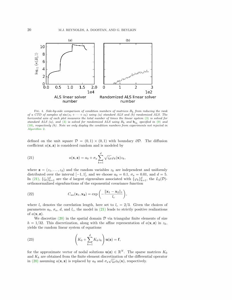
To better illustrate the behavior of the condition numbers in these experiments,we display condition numbers from a single experiment in Figure 4. Specifically,Figure 4(a) shows the condition number of the matrix Bk defined by (4) and used inAlgorithm 1, and Figure 4(b) shows the condition number of the non-rejected matrixBk defined by (9) and used in Algorithm 2. We emphasize that these plots contain thecondition numbers of all matrices Bk used in this experiment corresponding to eachdirectional update and ALS sweep. In Figure 4(a) we observe the condition number ofBk growing rapidly as the iteration number increases. Figure 4(b), however, displaysa milder increase in the condition number of Bk for the randomized ALS algorithm.

4.2. A manufactured tensor. Our next test is to compare the performanceof the standard and randomized ALS algorithms on a manufactured random tensorexample. To construct this example we generate factors by drawing M = 128 randomsamples from the standard Gaussian distribution. We chose d = 20 and set theseparation rank of the input tensor to r = 50. Then we normalized the factorsand set the s-values of the tensor equal to sl = e−l, l = 0, . . . , r − 1, where r waspredetermined such that send is small.

Similar to the sine example, we ran 500 experiments and requested an accuracyof ε = 10−4 from both algorithms. The maximum number of iterations for bothalgorithms was set to 1000, while the stuck tolerance for the standard ALS algorithmwas set to 10−6. We used the following parameters for the randomized ALS algorithm:the Bk matrices were of size (25 rF)× rF, and the repetition parameter, max tries inAlgorithm 2, was set to 50. We started all tests from randomized guesses with rankrF = 9 . This value was chosen because in all previous runs the reduced separationrank never fell below rF = 10. Such an experiment allows us to compare how thealgorithms perform when the initial approximation has rank greater than one.

We show in Figure 5 the output separation ranks from 500 tests of both therandomized and standard ALS algorithms. The CTD outputs from randomized ALShad, on average, lower separation ranks than those from standard ALS. Furthermore,as seen in Figure 5, some of the output CTDs from the standard ALS algorithm hadseparation rank of 40. In these instances, standard ALS failed to reduce the separationrank of the input CTD because simple truncation to rF = 35 would have given doubleprecision. These failures did not occur with the randomized ALS algorithm. We canalso see a contrast in performance in Figure 6: all tests of the randomized ALS


Fig. 1. Histograms displaying ALS reduction residuals, in log10 scale, for reducing the lengthof a CTD of samples of sin (z1 + · · · + z5). The experiments shown in (a) used randomized ALS,whereas the experiments shown in (b) used standard ALS. We note that both algorithms produceda small number of results with approximation errors worse than the requested tolerance. However,the randomized ALS method produced fewer results that did not meet our requested tolerance.

algorithm produced CTDs with reduced separation rank whose relative reductionerrors were less than the accuracy ε. Also, in Figure 6, we observe instances wherethe standard ALS algorithm failed to output a reduced separation rank CTD withrelative error less than ε.

There was a significant difference in the maximum condition numbers of matricesused in the two algorithms. In Figure 7, we see that matrices produced by standardALS had much larger condition numbers (by a factor of roughly 1010) than theircounterparts in the randomized ALS algorithm. Such large condition numbers mayexplain the failures of the standard ALS algorithm to output reduced separation rankCTDs with relative errors less than ε.

From Figure 8, we see that in most of the tests standard ALS required feweriterations than randomized ALS to converge. However, there were a few tests wherestandard ALS required a larger number of iterations. These are the tests that failed


Fig. 2. Histogram showing the maximum condition numbers from our experiments reducing thelength of a CTD of samples of sin (z1 + · · · + z5). The condition numbers are shown in log10 scale;the solid gray pattern represents condition numbers from standard ALS, while the hatch patternrepresents condition numbers from the randomized ALS algorithm.

Fig. 3. Histogram showing the number of iterations required by randomized ALS (hatch pat-tern) and the standard ALS algorithm (gray pattern) to reduce the length of a CTD of samples ofsin (z1 + · · · + z5).

to output a reduced separation rank CTD with relative error less than ε. We note thatsimilar to the experiments in subsection 4.1, the randomized ALS sweeps rejected byAlgorithm 2 are included in the iteration count.

4.3. Elliptic PDE with random coefficient. As the key application of therandomized ALS algorithm, we consider the separated representation of the solutionu(x, z) to the linear elliptic PDE

−∇ · (a(x, z)∇u(x, z)) = 1, x ∈ D,(20)

u(x, z) = 0, x ∈ ∂D,


Fig. 4. Side-by-side comparison of condition numbers of matrices Bk from reducing the rankof a CTD of samples of sin (z1 + · · · + z5) using (a) standard ALS and (b) randomized ALS. Thehorizontal axis of each plot measures the total number of times the linear system (3) is solved forstandard ALS (a), and (3) is solved for randomized ALS using Bk and bjk specified in (9) and(10), respectively (b). Note we only display the condition numbers from experiments not rejected inAlgorithm 2.

defined on the unit square D = (0, 1) × (0, 1) with boundary ∂D. The diffusioncoefficient a(x, z) is considered random and is modeled by

a(x, z) = a0 + σa

d∑k=1

√ζkϕk(x)zk,(21)

where z = (z1, . . . , zd) and the random variables zk are independent and uniformlydistributed over the interval [−1, 1], and we choose a0 = 0.1, σa = 0.01, and d = 5.In (21), {ζk}dk=1 are the d largest eigenvalues associated with {ϕk}dk=1, the L2(D)-orthonormalized eigenfunctions of the exponential covariance function

(22) Caa(x1,x2) = exp

(−‖x1 − x2‖1

lc

),

where lc denotes the correlation length, here set to lc = 2/3. Given the choices ofparameters a0, σa, d, and lc, the model in (21) leads to strictly positive realizationsof a(x, z).

We discretize (20) in the spatial domain D via triangular finite elements of sizeh = 1/32. This discretization, along with the affine representation of a(x, z) in zk,yields the random linear system of equations

(23)

(K0 +

d∑k=1

Kkzk

)u(z) = f ,

for the approximate vector of nodal solutions u(z) ∈ RN . The sparse matrices K0

and Kk are obtained from the finite element discretization of the differential operatorin (20) assuming a(x, z) is replaced by a0 and σa

√ζkφk(x), respectively.


Fig. 5. Histograms showing output ranks from experiments in reducing the length of CTDs. (a)shows ranks of CTDs output by the randomized ALS algorithm. (b) shows ranks of CTDs outputby the standard ALS algorithm. The CTDs output by the randomized ALS method typically have asmaller separation rank. In many examples the standard ALS algorithm required 40 terms, i.e. itfailed since truncation of the input tensor to rF = 35 should give double precision.

To fully discretize (23), we consider the representation of u(z) at a tensor-productgrid {(z1(j1), . . . , zd(jd)) : jk = 1, . . . ,Mk} where, for each k, the grid points zk(jk)are selected to be the Gauss-Legendre abscissas. In our numerical experiments, weused the same number of abscissas Mk = M = 8 for all k = 1, . . . , d. The discreterepresentation of (23) is then given by the tensor system of equations

(24) KU = F,

where the linear operation KU is defined as

KU =

d∑l=0

rU∑l=1

sUl

(Kl0Ul

0

)◦(Kl1Ul

1

)◦ · · · ◦

(KldUl

d

),

Kl0 = Kl,


Fig. 6. Histograms displaying ALS reduction errors, in log10 scale, for reduced-rank CTDs ofthe random tensor example. (a) shows that in our 500 tests, the randomized ALS method alwaysproduced a result that met the required tolerance. (b) shows how the standard ALS algorithm faredwith the same problem. Note that the standard ALS algorithm failed to reach the requested tolerancein a small number of tests.

and for k = 1, . . . , d,

Klk =

{D l = k

IM l 6= k,

where

D =

zk (1) 0. . .

0 zk (M)

,and IM is the M ×M identity matrix. The tensor F in (24) is defined as

F = f ◦ 1M ◦ · · · ◦ 1M ,


Fig. 7. Histogram showing the maximum condition numbers from experiments in reducing thelength of CTDs of the random tensor example. The condition numbers of Bk are shown in log10scale; solid gray represents condition numbers from standard ALS while the hatch pattern representscondition numbers from the randomized ALS algorithm. Similar to the sine example, the conditionnumbers from randomized ALS are much smaller than those from the standard ALS algorithm

where 1M is an M -vector of ones. We seek to approximate U in (24) with a CTD,

(25) U =

rU∑l=1

sUl

Ul0 ◦Ul

1 ◦ · · · ◦Uld,

where the separation rank rU will be determined by a target accuracy. In (25) Ul0 ∈

RN and Ulk ∈ RM , k = 1, . . . , d. To solve (24), we use a fixed point iteration similar

to those used for solving matrix equations and recently employed to solve tensorequations in [23]. In detail, the iteration starts with an initial tensor U of the formin (25). At each iteration i, U is updated according to

Ui+1 = (I−K) Ui + F,

while requiring ‖I−K‖ < 1. To assure this requirement is satisfied we solve

(26) Ui+1 = c (F−KUi) + Ui,

where c is chosen such that ‖I− cK‖ < 1. We compute the operator norm ‖I−K‖via power method; see, e.g., [4, 5].

One aspect of applying such an iteration to a CTD is an increase in the outputseparation rank. For example, if we take a tensor U of separation rank rU and use itas input for (26), one iteration would increase the rank to rF + (d+ 2) rU. Thereforewe require a reduction algorithm to decrease the separation rank as we iterate. Thisis where either the standard or randomized ALS algorithm is required: to truncatethe separated representation after we have run an iteration. Both ALS methods workwith a user-supplied truncation accuracy ε, so we denote the reduction operator asτε. Including this operator into our iteration, we have

(27) Ui+1 = τε (c (F−KUi) + Ui) .

Pseudocode for our fixed point algorithm is shown in Algorithm 3


Fig. 8. Histograms showing iterations required to produce reduced-length CTDs for the randomtensor example. (a) shows iterations required by randomized ALS, while (b) shows the iterationsrequired by the standard ALS algorithm. As seen in (b), a few examples using standard ALS requiredlarge numbers of iterations to output CTDs. These examples failed to produce a reduced separationrank CTD with relative error less than ε. However, for most of the experiments the standard ALSalgorithm required fewer iterations than the randomized ALS algorithm.

Remark 19. In this example, the separation rank of K is directly related to theproblem dimension d, i.e. rK = d + 1, which is a consequence of using a Karhunen-Loeve-type expansion for finite-dimensional noise representation of a(x, z). This willincrease the computational cost of the algorithm to more than linear with respect tod, e.g. quadratic in d when an iterative solver is used and N � M . Alternatively,one can obtain the finite-dimensional noise representation of a(x, z) by applying theseparated rank reduction technique of this study on the stochastic differential operatoritself to possibly achieve rK < d. The interested reader is referred to [3, 4] for moredetails.

First, we examine the convergence of the iterative algorithm given a fixed ALS reduc-tion tolerance in Figure 9. The randomized ALS method converges to more accuratesolutions in all of these tests (see Table 1). However, the ranks of the randomized ALS


Algorithm 3 Fixed point iteration algorithm for solving (27)

input : ε > 0, µ > 0, operator K, F, c, max iter, max rank, δ > 0(for standard ALS), max tries (for randomized ALS)

initialize rU = 1 tensor U0 = U11 ◦ · · · ◦U1

d with either randomly generatedU1k or U1

k generated from the solution of the deterministic versionof (20), i.e., when a(x, z) is replaced by a0 in (21). Also initializethe fixed point iteration counter to i = 0.

D0 = F−KU0

res = ‖D0‖ / ‖F‖while res > µ doi = i+ 1Ui = cDi−1 + Ui−1Ui = τε (Ui)Di = F−KUi

res = ‖Di‖ / ‖F‖end whilereturn Ui

ALS type ALS tol max κ (Bk) max rank rank residual

standard 1× 10−3 5.35× 101 5 4 4.16× 10−2

1× 10−4 5.29× 105 13 11 5.72× 10−3

1× 10−5 1.07× 109 37 34 4.18× 10−4

randomized 1× 10−3 2.59× 102 7 6 2.36× 10−2

1× 10−4 3.59× 103 22 19 2.35× 10−3

1× 10−5 2.72× 104 57 54 3.00× 10−4

Table 1Table containing ranks, maximum condition numbers, and final relative residual errors of ex-

periments with fixed ALS tolerance.

solutions are larger than the ranks required for solutions produced by the standardALS algorithm.

In Figure 10, we observe different behavior in the relative residuals using fixedranks instead of fixed accuracies. For these experiments the ALS-based linear solveusing the standard algorithm out-performs the randomized version, except in therank r = 30 case (see Table 2). In this case, the standard ALS algorithm has issuesreaching the requested ALS reduction tolerance, thus leading to convergence problemsin the iterative linear solve. The randomized ALS algorithm does not have the samedifficulty with the rank r = 30 example. This difference in decay between the standardand randomized ALS residuals corresponds to a significant difference between themaximum condition numbers of Bk. For the r = 30 case, the maximum conditionnumber of Bk matrices generated by randomized ALS was 3.94 × 107, whereas themaximum condition number of Bk matrices generated by standard ALS was 3.00 ×1013.


Fig. 9. Residual error versus fixed point iteration number of results from linear solvers. Theblack lines represent linear solve residuals where standard ALS was used for reduction, while thegray lines represent linear solve residuals where randomized ALS was used for reduction. In thethree examples shown above the ALS tolerances, for both standard and randomized ALS, were set to1× 10−3 for curves labeled (a), 1× 10−4 for curves labeled (b), and 1× 10−5 for curves labeled (c).

5. Discussion and conclusions. We have proposed a new ALS algorithm forreducing the rank of tensors in canonical format that relies on projections onto randomtensors. Tensor rank reduction is one of the primary operations for approximationswith tensors. Additionally, we have presented a general framework for the analysisof this new algorithm. The benefit of using such random projections is the improvedconditioning of matrices associated with the least squares problem at each ALS itera-tion. While significant reductions of condition numbers may be achieved, unlike in thestandard ALS, the application of random projections results in a loss of monotonicerror reduction. In order to restore monotonicity, we have employed a simple rejec-tion approach, wherein several random tensors are applied and only those that do notincrease the error are accepted. This, however, comes at the expense of additionalcomputational cost as compared to the standard ALS algorithm. Finally, a set ofnumerical experiments has been studied to illustrate the efficiency of the randomized


Fig. 10. Plots showing relative residuals of fixed point solutions versus fixed point iterationnumber. (a) two fixed point solutions are shown here: solutions for fixed ranks r = 10, and r = 20.Gray lines are residuals corresponding to reductions with randomized ALS and black lines correspondto reductions with the standard ALS algorithm. (b) One experiment with r = 30 and the same colorscheme as in (a).

ALS type ALS tol max κ (Bk) rank residual

standard 1× 10−5 9.45× 1011 10 7.29× 10−3

5× 10−6 1.27× 1013 20 1.97× 10−3

1× 10−6 3.00× 1013 30 4.73× 10−3

randomized 1× 10−5 9.39× 105 10 1.30× 10−2

5× 10−6 4.12× 106 20 2.93× 10−3

1× 10−6 3.94× 107 30 1.72× 10−3

Table 2Table containing maximum condition numbers and final relative residual errors of experiments

with fixed separation ranks.

ALS in improving numerical properties of its standard counterpart.The optimal choice of random variables to use in the context of projecting onto

random tensors is a question to be addressed in future work. In our examples wehave used signed Bernoulli random variables, a choice that worked well with both ournumerical experiments and analysis. On the other hand, there are limitations of sucha construction of random tensors, which motivate further investigations. A topic ofinterest for future work is the extension of the proposed randomized framework toother tensor formats including the Tucker, [24], and tensor-train, [28].

Another area of future work involves directly solving systems such as (24) witha randomized ALS variant, instead of utilizing a fixed point algorithm (e.g. Algo-rithm 3). A standard ALS algorithm for this purpose was derived in [4, Section 4.2],


where the approach is to solve AF = G by minimizing ‖AF−G‖ with an imposedseparation rank constraint on F. The resulting equations are also normal equationssimilar to (3) and (4), thus we anticipate our randomized machinery will extend tothis approach for solving AF = G.

Finally we have suggested an alternative approach to using projections onto ran-dom tensors that merits further examination. This approach uses the QR factoriza-tion to construct a preconditioner for the least squares problem at each ALS iteration.Hence it solves the same equations as the standard ALS, but the matrices have bet-ter conditioning. Also, because it solves the same equations, the monotonic errorreduction property is preserved. This is an important distinction from randomizedALS, which solves different linear systems, but the solutions to which are close to thesolutions from standard ALS.

Appendix A. Proofs of (6), Theorem 6, and Lemma 15. First, we prove(6).

Proof. To bound the condition number of AB we bound σmax (AB) from aboveand σmin (AB) from below. The bound we use of σmax (AB) is straightforward; itcomes from the properties of the two norm,

σmax (AB) ≤ σmax (A)σmax (B) .

To bound σmin (AB) we first note that AAT is nonsingular, and write σmin (AB) asfollows,

σmin (AB) =∥∥∥AAT (AAT )−1ABx∗

∥∥∥2,

where ‖x∗‖ = 1 is the value of x such that the minimum of the norm is obtained(see the minimax definition of singular values, e.g. [22, Theorem 3.1.2]). If we define

y = AT(AAT

)−1ABx∗, then

σmin (AB) =‖Ay‖ · ‖y‖‖y‖

≥ σmin (A) · ‖y‖ ,

from the minimax definition of singular values. To bound ‖y‖, we observe that

AT(AAT

)−1AB is the projection of B onto the row space of A. Denoting this

projection as PAT (B) we have,

‖y‖ = ‖PAT (B) x∗‖ ≥ σmin (PAT (B)) ,

since ‖x∗‖ = 1. Combining our bounds on the first and last singular values gives usthe bound on the condition number,

κ (AB) ≤ σmax (A)σmax (B)

σmin (A)σmin (PAT (B))= κ (A) · σmax (B)

σmin (PAT (B)).

The proof of Theorem 6 is broken down into three steps in order to control ‖Ax‖ forall x on the unit sphere: an approximation step, where the unit sphere is covered usinga finite epsilon-net N (see [32, Section 5.2.2] for background on nets); a concentrationstep, where tight bounds are applied to ‖Ax‖ for every x ∈ N ; and the final stepwhere a union bound is taken over all the vectors x ∈ N .

Proof. (of Theorem 6)


Vershynin observes that if we set B in Lemma 7 to A/√N , the bounds on the

extreme singular values σmin (A) and σmax (A) in (7) are equivalent to

(28)

∥∥∥∥ 1

NATA− I

∥∥∥∥ < max(δ, δ2

)=: ε,

where δ = C√

nN + t√

N. In the approximation step of the proof, he chooses a 1

4 -net

N to cover the unit sphere Sn−1. Evaluating the operator norm (28) on N , it issufficient to show

maxx∈N

∣∣∣∣ 1

N‖Ax‖22 − 1

∣∣∣∣ < ε

2,

with the required probability to prove the theorem.Starting the concentration step, [32] defines Zi = 〈Ai,x〉, where Ai is the i-th row

of A and ‖x‖2 = 1. Hence, the vector norm may be written as

(29) ‖Ax‖22 =

N∑i=1

Z2i .

Using an exponential deviation inequality to control (29), and that K ≥ 1√2, the

following probabilistic bound for a fixed x ∈ Sn−1 is,

P{∣∣∣∣ 1

N‖Ax‖22 − 1

∣∣∣∣ ≥ ε

2

}= P

{∣∣∣∣∣ 1

N

N∑i=1

Z2i − 1

∣∣∣∣∣ ≥ ε

2

}≤ 2 exp

[− c1K4

min(ε2, ε

)N]

= 2 exp[− c1K4

δ2N]≤ 2 exp

[− c1K4

(C2n+ t2

)],(30)

where c1 is an absolute constant.Finally, (30) is applied to every vector x ∈ N resulting in the union bound,

(31)

P{

maxx∈N

∣∣∣∣ 1

N‖Ax‖22 − 1

∣∣∣∣ ≥ ε

2

}≤ 9n · 2 exp

[− c1K4

(C2n+ t2

)]≤ 2 exp

(−c1t

2

K4

),

where we arrive at the second inequality by choosing a sufficiently large C = CK ([32]gives the example C = K2

√ln (9) /c1).

We now prove Lemma 15.

Proof. To prove this lemma we use the following inequality derived from (17),

(1− δ)2 ≤ σmin

(Σ−

12BTBΣ−

12

)≤ σmax

(Σ−

12BTBΣ−

12

)≤ (1 + δ)

2.

First we bound σmax (B) from above:

σmax (B)2 ≤

∥∥∥Σ12

∥∥∥ · ∥∥∥Σ−12BTBΣ−

12

∥∥∥ · ∥∥∥Σ12

∥∥∥≤∥∥∥Σ

12

∥∥∥2 · σmax

(Σ−

12BTBΣ−

12

)≤ σmax

(Σ

12

)2· (1 + δ)

2,


implying σmax (B) ≤ σmax

(Σ

12

)· (1 + δ) . Second we bound σmin (B) from below:

σmin (B)2

= σmin

(Σ

12 Σ−

12BTBΣ−

12 Σ

12

)≥ σmin

(Σ

12

)2· σmin

(Σ−

12BTBΣ−

12

)≥ σmin

(Σ

12

)2· (1− δ)2 ,(32)

implying σmin (B) ≥ σmin

(Σ

12

)·(1− δ) . The first inequality in (32) is from [22, prob.

3.3.12]. Finally, using properties of singular values we combine the inequalities:

σmin

(Σ

12

)· (1− δ) ≤ σmin (B) ≤ σmax (B) ≤ σmax

(Σ

12

)· (1 + δ) .

REFERENCES

[1] C. Appellof and E. Davidson, Strategies for analyzing data from video fluorometric moni-toring of liquid chromatographic effluents, Analytical Chemistry, 53 (1982), pp. 2053–2056.

[2] B. Bader, M. Berry, and M.Browne, Discussion tracking in enron email using parafac, inSurvey of Text Mining II, Springer London, 2008, pp. 147–163.

[3] G. Beylkin and M. J. Mohlenkamp, Numerical operator calculus in higher dimensions, Proc.Natl. Acad. Sci. USA, 99 (2002), pp. 10246–10251.

[4] G. Beylkin and M. J. Mohlenkamp, Algorithms for numerical analysis in high dimensions,SIAM J. Sci. Comput., 26 (2005), pp. 2133–2159.

[5] D. J. Biagioni, D. Beylkin, and G. Beylkin, Randomized interpolative decomposition ofseparated representations, Journal of Computational Physics, 281 (2015), pp. 116–134.

[6] R. Bro, Parafac. Tutorial & Applications., in Chemom. Intell. Lab. Syst., Special Issue 2ndInternet Conf. in Chemometrics (incinc’96), vol. 38, 1997, pp. 149–171.

[7] J. D. Carroll and J. J. Chang, Analysis of individual differences in multidimensional scalingvia an N-way generalization of Eckart-Young decomposition, Psychometrika, 35 (1970),pp. 283–320.

[8] Z. Chen and J. Dongarra, Condition number of gaussian random matrices, SIAM J. MatrixAnal. Appl., 27 (2005), pp. 603–620.

[9] P. Chew, B. Bader, T. Kolda, and A. Abdelali, Cross-language information retrievalusing parafac2, in Proceedings of the 13th ACM SIGKDD International Conference onKnowledge Discovery and Data Mining, KDD ’07, New York, NY, USA, 2007, ACM,pp. 143–152, http://dx.doi.org/10.1145/1281192.1281211.

[10] F. Chinesta, P. Ladeveze, and E. Cueto, A short review on model order reduction based onproper generalized decomposition, Archives of Computational Methods in Engineering, 18(2011), pp. 395–404.

[11] A. Doostan and G. Iaccarino, A least-squares approximation of partial differential equa-tions with high-dimensional random inputs, Journal of Computational Physics, 228 (2009),pp. 4332–4345.

[12] A. Doostan, G. Iaccarino, and N. Etemadi, A least-squares approximation of high-dimensional uncertain systems, Tech. Report Annual Research Brief, Center for TurbulenceResearch, Stanford University, 2007.

[13] A. Doostan, A. Validi, and G. Iaccarino, Non-intrusive low-rank separated approximationof high-dimensional stochastic models, Comput. Methods Appl. Mech. Engrg., 263 (2013),pp. 42–55.

[14] A. Edelman, Eigenvalues and condition numbers of random matrices, SIAM J. Matrix Anal.Appl., 9 (1988), pp. 543–560.

[15] A. Edelman, Eigenvalues and condition numbers of random matrices, ph.d. thesis, Mas-sachusetts Institute of Technology, 1989.

[16] G. Golub and C. V. Loan, Matrix Computations, Johns Hopkins University Press, 3rd ed.,1996.

[17] L. Grasedyck, D. Kressner, and C. Tobler, A literature survey of low-rank tensor approx-imation techniques, CoRR, abs/1302.7121 (2013).

http://dx.doi.org/10.1145/1281192.1281211


[18] W. Hackbusch, Tensor spaces and numerical tensor calculus, vol. 42, Springer, 2012.[19] M. Hadigol, A. Doostan, H. Matthies, and R. Niekamp, Partitioned treatment of un-

certainty in coupled domain problems: A separated representation approach, ComputerMethods in Applied Mechanics and Engineering, 274 (2014), pp. 103–124.

[20] N. Halko, P.-G. Martinsson, and J. A. Tropp, Finding structure with randomness: proba-bilistic algorithms for constructing approximate matrix decompositions, SIAM Review, 53(2011), pp. 217–288, http://dx.doi.org/10.1137/090771806.

[21] R. A. Harshman, Foundations of the Parafac procedure: model and conditions for an “ex-planatory” multi-mode factor analysis, Working Papers in Phonetics 16, UCLA, 1970.

[22] R. A. Horn and C. R. Johnson, Topics in matrix analysis, Cambridge Univ. Press, Cam-bridge, 1994.

[23] B. Khoromskij and C. Schwab, Tensor-structured Galerkin approximation of parametric andstochastic elliptic PDEs, SIAM Journal on Scientific Computing, 33 (2011), pp. 364–385.

[24] T. G. Kolda and B. W. Bader, Tensor decompositions and applications, SIAM Review, 51(2009), pp. 455–500, http://dx.doi.org/10.1137/07070111X.

[25] A. Nouy, A generalized spectral decomposition technique to solve a class of linear stochasticpartial differential equations, Computer Methods in Applied Mechanics and Engineering,196 (2007), pp. 4521–4537.

[26] A. Nouy, Generalized spectral decomposition method for solving stochastic finite element equa-tions: Invariant subspace problem and dedicated algorithms, Computer Methods in AppliedMechanics and Engineering, 197 (2008), pp. 4718–4736.

[27] A. Nouy, Proper generalized decompositions and separated representations for the numericalsolution of high dimensional stochastic problems, Archives of Computational Methods inEngineering, 17 (2010), pp. 403–434.

[28] I. V. Oseledets, Tensor-train decomposition, SIAM Journal on Scientific Computing, 33(2011), pp. 2295–2317.

[29] V. Rokhlin and M. Tygert, A fast randomized algorithm for overdetermined linear least-squares regression, in Proceedings of the National Academy of Sciences, vol. 105(36), Na-tional Academy of Sciences, September 2008, pp. 13212–13217.

[30] T. Sarlos, Improved approximation algorithms for large matrices via random projections, inFoundations of Computer Science, 2006. FOCS ’06. 47th Annual IEEE Symposium on,2006, pp. 143–152, http://dx.doi.org/10.1109/FOCS.2006.37.

[31] G. Tomasi and R. Bro, A comparison of algorithms for fitting the PARAFAC model, Comput.Statist. Data Anal., 50 (2006), pp. 1700–1734.

[32] R. Vershynin, Introduction to the non-asymptotic analysis of random matrices, in CompressedSensing, Theory and Applications, Y. Eldar and G. Kutyniok, eds., Cambridge UniversityPress, 2012, ch. 5, pp. 210–268.

[33] F. Woolfe, E. Liberty, V. Rokhlin, and M. Tygert, A fast randomized algorithm forthe approximation of matrices, Appl. Comput. Harmon. Anal., 25 (2008), pp. 335–366,http://dx.doi.org/10.1016/j.acha.2007.12.002.

http://dx.doi.org/10.1137/090771806

http://dx.doi.org/10.1137/07070111X

http://dx.doi.org/10.1109/FOCS.2006.37

http://dx.doi.org/10.1016/j.acha.2007.12.002

randomized alternating least squares for canonical tensor ...€¦ · randomized alternating least...

Documents