RandomizedKinodynamicMotion Planningwith Moving Obstacles

David Hsu�

RobertKindel� Jean-ClaudeLatombe�

StephenRock��Department of ComputerScience � Departmentof Aeronautics & Astronautics

Stanford University

Stanford, CA94305,U.S.A.

Abstract

This paperpresents a novel randomizedmotion planner for robots that must achieve aspecified goal underkinematic and/or dynamicmotion constraints while avoiding collisionwith moving obstacleswith known trajectories. The planner encodesthe motion constraintsontherobot with acontrol system andsamplestherobot’sstate� timespaceby picking controlinputsat randomandintegratingits equationsof motion. Theresult is aprobabilistic roadmapof sampledstate� time points, calledmilestones,connectedby shortadmissible trajectories.Theplannerdoesnot precomputetheroadmap;instead, for eachplanningquery, it generatesanew roadmapto connectan initi al anda goal state� time point. Thepaperpresentsa detailedanalysis of the planner’s convergencerate. It shows that, if the state� time spacesatisfies ageometric property called expansiveness, thena slightly idealized version of our implementedplanner is guaranteed to find a trajectory whenoneexists,with probability quickly convergingto 1, asthenumberof of milestonesincreases.Our planner wastestedextensively not only insimulatedenvironments,but alsoon a real robot. In thelatter case, a vision moduleestimatesobstaclemotionsjustbeforeplanning starts. Theplanneris thenallocatedasmall,fixedamountof time to compute a trajectory. If a change in theexpectedmotionof theobstaclesis detectedwhile therobotexecutes theplannedtrajectory, theplannerrecomputesa trajectory on thefly.Experimentsontherealrobot led to several extensionsof theplanner in orderto dealwith timedelays anduncertainties that areinherentto an integratedrobotic systeminteractingwith thephysical world.

1 Intr oduction

In its simplestform, motionplanningis apurelygeometricproblem:giventhegeometryof arobotandstaticobstacles,computea collision-freepathof therobotbetweentwo givenconfigurations.This formulationignoresseveral key aspectsof the physical world. In particular, robot motionsareoftensubjectto kinematicanddynamicconstraints(kinodynamic constraints[DXCR93]) thatcannotbe ignored. Unlike obstructionby obstacles,suchconstraintscannotbe representedasforbiddenregionsin theconfigurationspace.Moreover, theenvironmentmaycontainmovingob-stacles,requiring that computedpathsbe parametrizedby time to indicatewhenthe robot is to

1

Figure1: Robottestbedconsistingof anair-cushionedrobotamongmoving obstacles.

achieve a particularstate. In this paper, we considermotion planningproblemswith both kin-odynamicconstraintsandmoving obstacles,andproposean efficient algorithmfor this classofproblems.In practice,we alsoneedto considernumerousotherissues(e.g., uncertaintyabouttheenvironment),someof whichwill beexaminedhere.

Our work extendstheprobabilistic roadmap(PRM) framework originally developedfor plan-ning collision-freegeometricpaths[Kav94, KSLO96, Sve97]. A PRM plannersamplestherobot’sconfigurationspaceat randomandretainsthe collision-freesamplesasmilestones. It thentriesto connectpairsof milestoneswith pathsof predefinedshape(typically straight-linesegments inconfigurationspace)andretainsthecollision-freeconnectionsaslocal paths. Theresultis anundi-rectedgraph,calledaprobabilistic roadmap, whosenodesarethemilestonesandtheedgesarethelocal paths.Multi-query PRM plannersprecomputethe roadmap(e.g., [K SLO96]), while single-queryplannerscomputea new roadmapfor eachquery(e.g., [HLM97]). It hasbeenproventhat,underreasonableassumptionsaboutthegeometryof the robot’s configurationspace,a relativelysmallnumberof milestonespickeduniformly at randomaresufficient to capturetheconnectivityof theconfigurationspacewith highprobability [HLM97, KLMR95].

The plannerproposedin this paperrepresentskinodynamic constraintsby a control system,which is a setof differentialequationsthatdescribesall thepossible localmotions of a robot.Foreachquery, theplannerbuildsanew roadmapin thecollision-freesubsetof therobot’sstate� timespace,whereastatetypically encodesboththeconfigurationandthevelocity of therobot.To sam-ple a new milestone, it first selectsa control input at randomin thesetof admissible controlsandthenintegratesthecontrolsystemwith this input over a shortdurationof time, from a previouslygeneratedmilestone. By construction, thelocal trajectorythusobtainedautomaticallysatisfiesthekinodynamic constraints.If thistrajectorydoesnotcollidewith theobstacles,its endpointis addedto the roadmapasa new milestone. This iterative incrementalprocedureproducesa tree-shapedroadmaprootedat theinitial state� timepointandorientedalongthetimeaxis. It terminateswhena milestone falls in an “endgame”region from which it is known how to reachthe goal. Thisendgameregion may be specificallydefinedfor a given robot. It may alsobe generatedby theplannerby constructing asecondtreeof milestonesrootedat thegoalandintegratingtheequationsof motion backwardsin time.

2

Our plannerexploits thesynergy of previously proposedideas(seeSection2). It makestwokey contributions,onetheoreticalandoneexperimental:

� We provide an in-depthanalysisof the planner’s convergencerate. It shows that, if thestate� timespacesatisfiesageometricpropertycalledexpansiveness, thenundersuitableas-sumptions,theprobabilitythattheplannerfails to find a trajectory, whenoneexists,quicklygoesto 0, asthenumberof milestonesincreases.Theexpansivenesspropertydefinedheregeneralizesa similar notion introducedin [HLM97] for holonomic robotsin staticenviron-ments.Theproofof convergence,however, is differentfrom theonein [HLM97] . Theearlierproofassumesthatlocalmotionsof therobotaretotally unconstrained.It alsocritically usesthesymmetry of theconnectivity relationshipin configurationspace—ifa point � is reach-ablefrom a point � , then � is alsoreachablefrom � . This symmetricrelationship no longerholdswhentherobothasanasymmetriccontrolsystem(e.g., a car-like robotthatcanonlymove forward)or whenobstaclesaremoving. Currentlywe do not know how to estimateapriori thedegreeof expansivenessfor agivenstate� timespace.Hence,ouranalysisis onlyonesteptowardunderstandingtheconvergenceof randomizedmotion planners.However,webelievethatexpansivenessis averyusefulconceptfor characterizingthespacesin whichrandomizedplannersarelikely to work well (or not sowell). It mayalsohelpin designingbettersamplingstrategies.

� We alsodescribesour experiencesin integrating the plannerinto a hardwarerobot testbed(Figure1). In this integratedsystem,avisionmoduleestimatesobstaclemotionsjustbeforeplanningstarts. The planneris thenallocateda small, fixed amountof time (a fraction ofa second)to computea trajectory. If a changein the expectedmotion of the obstaclesisdetectedwhile therobotexecutestheplannedtrajectory, theplannerrecomputesa trajectoryonthefly. Experimentsontherealrobotled to severalextensionsof theplannerto dealwithtime delaysanduncertaintiesthat are inherentto an integratedrobotic systeminteractingwith thephysicalworld. This is particularlyimportantbecausekinodynamic constraintsarenotoriously difficult tomodelaccurately. Evenmoredifficult is tobuild anaccuratemodelforpredictingfutureobstaclemotion. Our experimentalwork demonstratesthata fastplannercanreliably handledynamicenvironments, even with uncertaintyin the future motionsoftheobstacles.

Therestof thepaperis organizedasfollows. Section2 reviewspreviouswork. Section3 describestheplanningalgorithm. Section4 developsthe theoreticalanalysisof theplanner’s convergence.Sections5 through7 describeour experiments with the planneron a nonholonomic robot andon a dynamically-constrainedrobot developedto investigatespaceroboticstasks. In simulation(Sections5 and6), we verified that the plannercanreliably solve tricky problems. In the hard-warerobottestbed(Section7), we verifiedthattheplannercanoperateeffectively despitevariousuncontrollableuncertaintiesandtimedelays.

This papercombinesandextendsthe resultspreviously reportedin [HKLR00, KHLR00]. Formoredetails,see[Hsu00, Kin01].

3

2 PreviousWork

2.1 Motion planning by random sampling

Sampling-basedmotionplanningis aclassicconceptin motionplanning(e.g., see[Don87]). Orig-inally, theapproachwasproposedto bothavoid difficultiesencounteredin implementingcompleteplanners(e.g., floating-pointapproximations) andfacilitatethe incorporationof searchheuristics(e.g., potentialfields).Samplesareorganizedinto regulargridsor hierarchicalones(e.g., quadtreesin 2-D configurationspaces).Thesegrids provide an explicit representationof the robot’s freespaceandhelpthesearchalgorithmto rememberthepoints alreadyvisited. Their size,however,growsexponentially with thedimensionalityof theconfigurationspace,i.e., thenumberof degreesof freedom(dofs)of therobot.Moreover, explicitly computingthegeometryof thefreesubsetof aconfigurationspacewith dimension greaterthanfour or five turnsout to have a prohibitively highcost.

Randomsampling—morespecifically, PRM methods—was introducedto solve (geometric)path planningproblemsfor robotswith many dofs [ABD 98, BK00, BKL 97, BL91, BOvdS99,HLM99, HST94,Hsu00, Kav94, KSLO96, Kuf99, LH00, SLL01, Sve97]. The costly computation ofan explicit representationof the free spaceis replacedby a collision test on every randomlypicked sampleandconnectionbetweensamples.This, of course,canbe donewith regular andhierarchicalgrids, too. More interestingly, randomsamplingprovidesan incrementalplanningschemewhich doesnot artificially dependon thedimensionality of theconfigurationspace.Theanalysisof the convergencerate of several PRM algorithms reveals the true value of randomsampling[Hsu00, HLM97, KKL 98, KLMR95, Sve97]: eachnew milestone addedto a probabilis-tic roadmap refinesthe theconnectivity relationship capturedin andreducestheprobabilitythattheplannerfails to find a solution path,whenoneexists(seeSection2.3).

Variousapplicationsof randomizedplannersarereviewed in [Lat99], including robotics,de-sign for manufacturingandservicing,graphicanimation of digital actors,surgical planning,andpredictionof molecularmotion.

Otherplanningapproaches(e.g., [Ahu94, HXCW98]) attemptto capturetheglobalconnectivityof a robot’s freespaceby combiningexplorationandsearchin amannersimilar to graphsearchinartificial intelligence.

2.2 Sampling strategies

ProposedPRM techniquesdiffer in their sampling strategies. An importantdistinction existsbe-tweenmulti-querystrategies(e.g., [K SLO96]) andsingle-queryones(e.g., [HLM97]). A multi-queryplannerprecomputesa roadmapfor a given robot andworkspaceandthenusesthis roadmaptoprocessmultiple queries.In general,thequeryconfigurationsarenot known in advance.So thesamplingstrategy mustdistribute themilestonesover the entirefree space.In contrast,a single-queryplannercomputesa new roadmapfor eachquery. Herethe goal is to find a collision-freepathbetweenthe two queryconfigurationsby exploring aslittl e spaceaspossible. Multi-querystrategiesareappropriatewhenthecostof precomputing a roadmapcanbeamortizedovera largenumberof queries.Single-queryonesareappropriatewhenthenumberof queriesin agivenspaceis small. Intermediatestrategies,which precomputepartial roadmapsandcompletethemto pro-

4

cessspecificqueries,havealsobeenproposed[BK00, SMA01]. Theplannerproposedin thispaperfollowsthesingle-querysampling paradigm.

Single-querystrategiesoftenbuild anew roadmapfor eachqueryby growing treesof sampledmilestonesrootedat the initial and/orgoal configurations[AG99, HLM97, Hsu00, Kuf99, LK99],but they differ in theway they samplethemilestonesthat form thenodesof the trees.Similar totheplannerin [HLM97] , our algorithmselectsa milestone� in a treeto expandat random,withprobability inverseproportionalto the currentdensityof milestonesaround � (seeSection3.2).A new milestoneis thenpickedby samplingtheneighborhood of � at random.This guaranteesthat the roadmapeventually diffusesthroughthe component(s)of the free spacereachablefromthequeryconfigurationsandthatthemilestonedistribution over thesecomponentsconvergesto auniform one. This condition is neededfor theanalysisof theplanner’s convergencedevelopedinSection4. An alternative is to first pick a configuration� in the configurationspaceat random,select� to bethemilestone in thetreeclosestto � , andthenpick a new milestonealongthe lineconnecting� to � [LK99]. This techniqueis slightly simplerto implement thanoursandworkswell whenthequeryadmitsa solution thatdoesnot requirelong detours.However, this samplingstrategy biasesthedistribution of milestonestowardthoseregionsin theconfigurationspacewithlarge obstacles.This maybe undesirableandseverelyslow down the rateof convergenceof theplanner. Anotherpossibility is to grow thesearchtreeby pickingeachnew milestoneasfarawayaspossible from thecurrentmilestones[AG99]. Othertechniquesor refinementsof thesetechniquesareclearlypossible. Ourexperienceis that,althoughonemayimprove theperformanceof aPRMplanneronsomeexamplesby biaising thedistributionof milestones,asamplingstrategy thatyieldsa uniform distribution of milestonesover the reachablefree spaceavoids pathological casesandgivesthebestresultson theaverage.

2.3 Probabilistic completeness

A completemotion planneris onethat returnsa solution whenever oneexists andindicatesthatno suchpathexistsotherwise.However, aswasshown in [Rei79], pathplanning is PSPACE-hard,which is strongindication that any completeplanneris likely to be exponential in the numberof dofs of a robot. Adding kinodynamic constraintsandmoving obstaclesfurther increasesthecomplexity of theproblem[DXCR93,RS85].

A plannerbasedon randomsamplingcannotbecomplete.However, a weaker notionof com-pleteness,calledprobabilistic completeness,was introducedin [BL91]: a planneris probabilis-tically completeif the probability that it returnsa correctanswergoesto 1 asthe runningtimeincreases.Supposethata randomizedplannerreturnsa solution pathassoonasit findsone,andindicatesthatnosuchpathexistsif it cannotfoundoneafteragivenamountof time. If theplannerreturnsapath,theanswermustbecorrect.If it reportsthatnopathexists,theanswermaybesome-timeswrong.It hasbeenshown thattheprobability thattherandomizedpotential field plannerfailsto find a solution pathwhenoneexistsgoesto 0 astherunningtime increases,henceproving thatthe planneris probabilistically (resolution)complete[BL91]. Several otherrandomizedplannershavealsobeenprovento beprobabilistically complete[AG99, LK01, LL96, Sve97].

Probabilisticcompleteness, however, is a weakconcept,as it saysnothing abouta planner’srateof convergence.In orderto understandwhy PRM plannerswork well in practiceandidentifythecaseswherethey maynot work well, we needto show that they have a fastconvergencerate.

5

This requiresus to develop a characterizationof the complexity of the input geometrythat issuitablefor randomsampling. This characterizationshouldnot dependon the dimensionality oftheconfigurationspacein anartificial way. After all, is it reallymoredifficult to sampleanempty� -dimensionalhypercubethanto sampleanemptysquare?Along theselines, it hasbeenshownthat,undersuitableassumptions,certainidealizedversionsof multi-queryPRMpathplannershavea convergencerateexponential in the numberof sampledmilestones[HLM97, HLMK99, KKL 98,KLMR95, Sve97, SO98].

More specifically, thenotionof -goodnesswasintroducedto characterize thecomplexity ofa robot’s configurationspace[KLMR95, BKL 97]. If a spaceis -good, thenwith somelimitedhelp from a completeplanner, a multi-queryPRM plannerthat samplesmilestonesuniformly atrandomfrom theconfigurationspaceconvergesat anexponentialratewith respectto thenumberof sampledmilestones.The proof of this result relatesPRM methodsto the issueof visibilitysetsstudiedin computational geometry, in particular, theart-gallery problem[O’R97]: eachmile-stoneis regardedasa guardthatseesa subsetof therobot’s freespace,themilestone’s visibilityregion [KLMR95] . This insight wasrecentlyexploitedto generatesmallerroadmaps[SLL01].

To remove theneedfor a completeplannerin theproof presentedin [BKL 97], expansivenesswasintroducedasa morerefinedcharacterizationof the robot’s free space.While the computa-tional complexity of a completeplanneris usuallyexpressedasa functionof thenumberof dofsand the numberand the degreeof polynomials describingthe boundarysurfaceof a robot andobstacles,therateof convergenceof aPRM planneris expressedasa functionof parametersmea-suringthedegreeto which a robot’s freespaceis expansive. Importantly, theexpansivenessof afree spacecapturesthe “narrow passage”issuestudiedin [HKL 98]. It revealsthe true narrow-nessof a passageandis a bettermeasurethanthewidth of thepassageto capturethedifficulty ofsamplingin amulti-dimensionalnarrow passage[HLM99] .

In this paper, we further generalizethe notion of expansivenessandextend it to state� timespace.Weprovethatif thestate� timespaceisexpansive, thenundersuitableassumptions,ournewrandomizedplannerfor kinodynamicplanningwith movingobstaclesis probabilistically completewith aconvergencerateexponentialin thenumberof sampledmilestones.

2.4 Geometric complexity

Onetenetof thePRMapproachto motionplanningis thata fastalgorithm existsto checksampledconfigurationsandconnectionsbetweenthemfor collision. Whenboththerobotandtheobstacleshavesimplegeometricshapes,which is thecaseof mostexamplesin thispaper, thisassumption isclearlysatisfied.However, doesthis remaintruewhentherobotandtheobstaclesarecomplex 3Dobjectsdescribedby 100,000trianglesor more?

During the pastdecade,a numberof efficient collision checkingand distancecomputationalgorithms have beendeveloped. The most popularonesare hierarchicaldecomposition algo-rithms, which precomputea multi-level boundingapproximation of every object in an environ-ment,usingprimitivevolumessuchasspheres,axis-alignedboundingboxes,or orientedboundingboxes[CLMP95,GLM96, Hub96, KHM 98,KPLM98, Qui94]. Experimentsreportedin [SA01] indi-catethatthePQPpackage[GLM96] teststwo objects,describedby 500,000triangleseach,in timesrangingbetween0.0001and0.0025seconds(onanIntel PentiumIII 1GHzprocessor),dependingon theactualdistancebetweenthetwo objects.

6

The useof efficient collision checkers in PRM plannershasbeenreportedin [BK00, CL95,HLM97, SA01,SLL01]. Theseplannersarecapableof efficiently andreliably processingplanningquerieswith geometricmodelscontaininghundredsof thousandsof triangles.

2.5 Moving obstacles

Whenobstaclesaremoving, theplannermustcomputea trajectoryparametrizedby time, insteadof simplyageometricpath.Thisproblemhasbeenprovento becomputationally difficult evenforrobotswith few dofs[RS85].

A numberof heuristic algorithms(e.g., [FS96,Fuj95, KZ86]) havebeenproposed.Thetechniquein [KZ86] is a two-stageapproach:in thefirst stage,it ignoresthemovingobstaclesandcomputesacollision-freepathof therobotamongthestaticobstacles;in thesecondstage,it tunestherobot’svelocityalongthis pathto avoid colliding with moving obstacles.Theresultingplanneris clearlyincomplete,but it oftengivesgoodresultswhenthenumberof moving obstaclesis smalland/orthe workspaceis not too cluttered. The plannerin [Fuj95] tries to reducethe incompletenessbygeneratinga network of paths.Theplannerin [FS96] introducesthenotion of a velocity obstacle,definedasthesetof velocitiesthatwill causetherobotto collidewith anobstacleat a futuretime.Velocity obstaclesareusedto generatean initial feasibletrajectoriesfor therobot,which is lateroptimized.Theplannercanhandleactuatorconstraintssuchasboundedacceleration.

Thenotionof a configuration� time spacewasintroducedin [ELP87] to coordinatethemotionof multiple robots. It was later extendedin [Fra93] to that of a state� time space,wherea stateencodesa robot’s configurationandvelocity, to plan robot motions with both moving obstaclesandkinodynamicconstraints.

2.6 Kinematic and dynamic constraints

Kinodynamic motionplanningrefersto problemsin which the robot’s motion mustsatisfynon-holonomic and/ordynamic constraints.

Planningfor nonholonomicrobotshasattractedconsiderableinterest(e.g., [BL89, Lau86, LCH89,LJTM94, LM96, SO94,SSLO97]). Oneapproach[Lau86, LJTM94] is to first generatea collision-free path,ignoring the nonholonomic constraints,andthenbreakthis pathinto small piecesandreplacethem by admissible canonicalpaths(e.g., ReedsandSheppcurves [RS90]). An exten-sion is to performsuccessive pathtransformationsof varioustypes[Fer98, SL98]. A relatedap-proach[SSLO97,SO94]usesa multi-queryPRM algorithmthatconnectsmilestonesby canonicalpathsegmentssuchasReedsandSheppcurves.All thesemethodsrequiretherobotsto belocallycontrollable[BL93, HK77, LCH89,LM96]. An alternativeapproach,introducedin [BL89, BL93], isto generatea treeof sampledconfigurationsrootedat theinitial configuration.At eachiteration,asampleis selectedfrom thetreeandexpandedto producenew samples,by integratingtherobot’sequationsof motionover a shortdurationof time with deterministically pickedcontrols.A spacepartitioningschemeregulatesthedensityof samplesin any regionof theconfigurationspace.Thisapproachworkswell for car-like robotsandtractor-trailor robotswith two to four dofsandis ap-plicableto robotsthatarenot locally controllable. Our new plannertakesa similar approach,butpickscontrolsat random.Neithertheplannernor theanalysisof its convergenceraterequirestherobot to be locally controllable. Comparedto theplannerin [BL93] andtheplannerpresentedin

7

this paper, thetwo-stepapproachof [Lau86, LJTM94] hastheadvantagethat it canreachthegoalconfigurationexactly, which eliminatestheneedto defineanendgameregion, but it is applicableonly to locally controllablerobots.

Algorithms for dealingwith dynamicconstraintsarecomparableto thosedevelopedfor non-holonomic constraints. In [BDG85, SD91], a collision-freepath is first computed,ignoring thedynamicconstraints; avariational techniquethendeformsthispathinto a trajectorythatbothcon-formsto thedynamicconstraintsandoptimizesacriterionsuchasminimal executiontime. Thesemethodswork well onmany practicalexamples;however, noformalguaranteeof performancehasbeenestablishedfor them. In fact, it is not alwayspossible to transformthepathgeneratedin thefirst phaseinto an admissible trajectory, dueto limits on the actuatorforcesor torques.The ap-proachin [DXCR93] placesaregulargrid over therobot’sstatespaceanddirectlysearchesthegridfor anadmissible trajectoryusingdynamicprogramming. It offersprovable performanceguaran-tees(resolution completenessandan asymptotic boundon the computation time), but it is onlyapplicableto robotswith few dofs(typically, two or three),asthesizeof thegrid grows exponen-tially with the numberof dofs. The plannerin [Fra93] usesa similar approachin the state� timespaceof the robot and dealswith moving obstaclesas well. Both our plannerand the one in[Kuf99, LK99, LK01] have many similaritieswith the approachtaken in [BL93, DXCR93, Fra93].Our plannerdiscretizesthe state� time spacevia randomsampling,insteadof placinga regulargrid over it. This makesit possible to dealwith robotswith many moredofs. On theotherhand,our plannerdoesnot achieve resolutioncompletenessas the one in [DXCR93]. Instead,undersuitableassumptions,it achievesprobabilistic completenesswith anexponential convergencerate(Section4).

The representationand the algorithm usedin our plannerbuild uponseveral existing ideas,in particular: single-queryrandomsamplingof configurationspace[HLM97] , state� time spaceformulation[BL93, DXCR93,ELP86,Fra93], andrepresentationof kinodynamic constraintswith acontrolsystem[BL93, DXCR93, Fra93]. Themostsalientcontributionsof thiswork arethegeneral-izationof expansivenessto state� timespace,thetheoreticalanalysisof theplanner’sconvergencerate,andtheintegrationandexperimentsof theplannerona realrobot.

3 Planning framework

Ouralgorithmbuildsaprobabilistic roadmapin thecollision-freesubset� of thestate� timespaceof therobot.Theroadmapis computedin theconnectedcomponentof � thatcontainstherobot’sinitial state� time point.

3.1 State-spaceformulation

Motion constraintsWeconsidera robotwhosemotion is governedby anequationof theform

������������������ (1)

where � �"! is therobot’s state,�� is its derivative relative to time,and �"�$# is thecontrolinput.

Thesets! and # aretherobot’sstatespaceandcontrol space, respectively. Weassumethat ! and

8

%

&

'

(

)

*

+

Figure2: A simple modelof acar-like robot.

# areboundedmanifoldsof dimensions � and � with �-, � . By definingappropriatecharts,wecantreat ! and # assubsetsof R. andR/ .

Eq. (1) can representboth nonholonomic and dynamic constraints. The motion of a non-holonomic robot is constrainedby 0 independent,non-integrablescalarequationsof the form132 � � � �� �4�65 , 7 � 89��:;�=<><=<?� 0 , where � and

�� denotethe robot’s configurationandvelocity, re-spectively. Define the robot’s stateto be �$� � . It is shown in [BL93] that, underappropriateconditions, the constraints

1�2 �@�9� ��A�B�C5D� 7 �E89��:;�><=<=<F� 0 areequivalent to Eq. (1) in which � is avectorin R/ � R.HGJI . In particular, Eq. (1) canberewrittenas 0 ���LK � independentequationsof the form

132 ���9� ��M� �N5 . Dynamicconstraintsarecloselyrelatedto nonholonomic constraints.In Lagrangianmechanics,dynamicsequationsareof the form 2 � � � �� �DO� �P�-5 , where � , �� , andO� aretherobot’s configuration,velocity, andacceleration,respectively. Definingtherobot’s stateas �L�Q� � � �� � , we canrewrite the dynamicsequationsin the form

1R2 ���9� ��A�S�T5 , which, asin thenonholonomic case,is equivalentto Eq.(1).

Robotmotionsmayalsobeconstrainedby inequalitiesof theforms1U2 � � � �� � , 5 and 2 � � � �� �;O� � ,5 . These-constraintsrestrictthesetsof admissible statesandcontrolsto subsetsof R . andR/ .

ExamplesThesenotionsareillustratedbelow with two examplesthatwill alsobeusefullater inthepaper:

Nonholonomic car navigation. Considerthecarexamplein Figure2. Let �WVX��YZ� bethepositionofthe midpoint [ betweenthe rearwheelsof the robot and \ be the orientationof the rearwheelswith respectto the V -axis.Definethecar’sstateto be �WVX�]Y^� \ �U� R_ . Thenonholonomicconstraint`baHc \ � �YDd �V is equivalentto thesystem

�V � egf>h9i \�Y � egi�j c \�\ � �We;dlkm� `balcon <Thisreformulationcorrespondstodefiningthecar’sstatetobeitsconfiguration�WVX��Yp� \ � andchoos-ing thecontrol input to bethevector �qer� n � , where e and

narethecar’s speedandsteeringangle.

9

Boundson �sVX�]Y^� \ � and �qer� n � canbeusedto restrict ! and # to subsetsof R _ andRt , respectively.For instance,if themaximumspeedof thecaris 1, thenwehave u e uv, 8 .Point-massrobot with dynamics. For a point-massrobot w moving on a horizontalplane,wetypically want to control the forcesappliedto w . This leadsus to definethe stateof w as �x��WVX��Yp�]eMy9��e{z>� , where �sVX�]YD� and �qeMy��]eMz>� aretheposition andthevelocity of w . Thecontrol inputsarechosento betheforcesappliedto w in the V - and Y -direction. Hencetheequationsof motionare �V � eMy �eMy � �ryAd ��Y � eMz �e{z � �rz>d � � (2)

where� is themassof w and �W�^y9���rz>� is theappliedforce.Thevelocity �qely9�]e{z=� andforce �q�|yl�]�|z>�arerestrictedto subsetsof Rt dueto limits on themaximumvelocityandforce.

Planning query Let !U} denotethe state� time space! ��~ 5;������� . Obstaclesin the robot’sworkspacearemappedinto this spaceasforbiddenregions.The freespace�-� !�} is thesetofall collision-freepoints ���9����� . A collision-freetrajectory ��� ��� ~ �>�F��� t

���� � �W���o�C���J�s���F������� � isadmissible if it is inducedby a function � �M~ �=���b� t

�p� # throughEq.(1).A planningqueryis specifiedby an initial state� time �@�9�]������� anda goal state� time ���M�M�����?� .

A solution to thequeryis eithera function � �M~ ��������� ��� # that inducesa collision-freetrajectory��� �L� ~ ���]����� ���� � �s�������@�v�W����������� � , suchthat �J�s�������Q�=� , �v�W���?���Q�>� , or an indicationthatno admissible trajectoryexistsbetween�@�H�]������� and �@�>�M�����?� . This formulationcanbeextendedtoallow ��� to beany instantin somegiven time interval, or to betheearliestpossiblearrival time.

In thefollowing, weconsiderpiecewise-constantfunctions���W��� only.

3.2 The planning algorithm

Ourplanningalgorithmis anextensionof thealgorithmpresentedin [HLM97] . It iteratively buildsa tree-shapedroadmap� rootedat � �L� ���=�b������� . At eachiteration, it first picks at randomamilestone �@�9����� from � , a time ��� with ��� , ��� , and a control function � �A~ ������� ��� # . It thencomputesthe trajectoryinducedby � by integrating Eq. (1) from �@�9����� . If this trajectorylies in� , its endpoint �@�M� �����¡� is addedto � asa new milestone;a directededgeis createdfrom �@�9����� to�@� � ��� � � , and � is storedwith this edge. The kinodynamic constraintsare thusnaturallyenforcedin all trajectoriesrepresentedin � . The plannerexits with successwhen the newly generatedmilestonefalls in an“endgame”region thatcontains�@�H�M�����?� .Milestone selectionThe plannerassignsa weight ¢ � � � to eachmilestone � in � . The weightof � is thenumberof othermilestoneslying in theneighborhoodof � . So ¢ � � � indicateshowdenselythe neighborhoodof � hasalreadybeensampled.At eachiteration, the plannerpicksan existing milestone � in � at randomwith probability £�¤ � � � inverselyproportionalto ¢ � � � .Hence,a milestonelying in a sparselysampledregion hasa greaterchanceof beingselectedthana milestonelying in analreadydenselysampledregion. This techniqueavoidsoversampling anyparticularregionof � .

Control selectionLet ¥§¦ be the set of all piecewise-constant control functionswith at most ¨constantpieces. So every �©� ¥�¦ admitsa finite partition ��ª¬«N�]�­«®<=<><�«E� ¦ suchthat �§�s���is a constant

2 �°# over the time interval �W� 2 G �����2 � , for 7 � 89��:;�><=<=<F� ¨ . We also require � 2 K

10

� 2 G � ,®±�²X³@´ , where ±�²X³@´ is a constant. Our algorithmpicks a control �µ� ¥U¦ , for somepre-specified and ±F²X³@´ , by sampling eachconstantpieceof � independently. For eachpiece, ¯ 2 and± 2 �¶� 2 K·� 2 G � areselecteduniformly at randomfrom # and ~ 5D� ±>²X³@´ � , respectively. The specificchoicesof theparameters and ±F²X³@´ will bediscussedin Section4.5. In theactualimplementationof thealgorithm, however, onemaychose �¸8 , becauseany trajectorypassingthroughseveralconsecutivemilestonesin thetree � is obtainedby applyingasequenceof constantcontrols.

EndgameconnectionUnlike someotherplanningtechniques(e.g., [Lau86, LJTM94]), theabove“control-driven” samplingtechniquedoesnot allow usto reachthegoal ���9�M�����?� exactly. We needto “expand” the goal into an endgameregion that the samplingalgorithmwill eventually attainwith highprobability. Thereareseveralwaysof creatingsucha region:� In [BL93], theendgameregionis definedto beaball of smallradiuscenteredatthegoal.Any

point in thisball is consideredto beasufficiently goodapproximation of thespecifiedgoal.This techniqueis practicalonly in spacesof small dimensionality, as the relative volumeof a ball of small fixed radiusgoestoward 0 as the dimensionality increases.We couldneverthelessadaptthis techniqueby settingtheparameter±M²X³@´ proportionalto thedistancebetweenthe milestone picked from � andthe goal, allowing the densityof milestonestoincreasein thegoal’svicinity, andterminating with successwhentheplannersamplesanewmilestonecloseenoughto thegoal.

� For somerobots,it is possible to analyticallycomputeoneor severalcanonicalcontrolfunc-tionsthatexactly connecttwo given pointswhile obeying thekinodynamicconstraints.Anexampleis theReedsandSheppcurves[RS90]developedfor nonholonomiccar-like robots.If suchcontrol functionsareavailable,onecantestif a milestone � belongsto theengameregionby checkingwhetheracanonicalcontrolfunctiongeneratesacollision-freetrajectoryfrom � to �@�=�M�����?� .

� A moregeneralmethodis to build a secondarytree � � of milestonesfrom the goal in thesamewayasthatfor theprimarytree � , exceptthatEq.(1) is integratedbackwardsin time.Let ���=� �����¹� beanew milestoneobtainedby integratingbackwardsfrom anexistingmilestone��������� in � � . By construction,if thetime goesforward,thecontrol functiondrivestherobotfrom state� � at time � � to state� at time � (Figure3). Thusthereis a known trajectoryfromevery milestone in � � to the goal. The sampling processterminateswith successwhenamilestone � � � is in theneighborhoodof a milestone � � � � � . In this case,theendgameregionis theunionof theneighborhoodsof milestonesin � � . To generatethefinal trajectory,we simply follow theappropriateedgesof � and � � ; however, thereis a smallgapbetween� and � � . Thegapcanoftenbedealtwith in practice.For example,beyond � , onecanusea PD controllerto trackthetrajectoryextractedfrom � � . Constructingendgame regionsbybackwardintegrationis averygeneraltechniqueandcanbeappliedto any systemdescribedby (1).

In Sections5–7, we will presentimplementationsof the planner, using the last two techniquesdescribedabove.

Endgameregion canalsobe usedwhenthe goal doesnot have a uniqueconfiguration. Forexample,in [AG99], the goal region is definedto be the subsetof configurationsof a redundantrobotsuchthattheend-effectorachievesagivenposture.

11

º

º�» ¼¾½�¼�¿�À�Á� Ã=ÄÁ�ÂÆÅX¼§ÇbÃ>ÂÆÄ�Ç�ÈÉÃFÊÌË|Í]ÊÏÎÐFÑ ÍFÄFÄ�ÂÆÄ�ÇÁ�ÂÆÅX¼3Ç�Ã>ÂÆÄ�Ç�Ò]Í]¿�Ó�ËZÍbÊÏÎ

ÔÔ »

Figure3: Building asecondarytreeof milestonesby integratingbackwardsin time.

Algorithm in pseudo-codeTheplanningalgorithmis summarizedin thefollowing pseudo-code.

Algorithm 1 Control-drivenrandomizedexpansion.1. Insert � � into � ; 7�Õ 8 .2. repeat3. Pick amilestone � from � with probability £Ö¤ � � � .4. Pick acontrolfunction � from ¥�¦ uniformly at random.5. � � Õ PROPAGATE � � �]�p� .6. if � �§×�ÙØ|ÚsÛ then7. Add � � to � ; 7�Õ 7 �Ü8 .8. CreateanedgeÝ from � to � � ; store� with Ý .9. if � �^� ENDGAME then exit with SUCCESS.10. if 7 �ßÞ then exit with FAILURE.

In line 5, PROPAGATE � � �]�p� integratestheequationsof motion from � with control � . It returnsanew milestone � � if thecomputedtrajectoryis admissible; otherwiseit returnsnil. If thereexistsno admissible trajectoryfrom � �o�¸�@�=�]������� to ���=�M�����?� , thealgorithmcannotdetectit. Therefore,in line 10, we boundthe maximumnumberof milestonesto be sampledby a constantÞ . TheoutcomeFAILURE maybeinterpretedas“thereexistsnosolution trajectory”,but thisanswermaybeincorrect.

Theabove algorithmcanpotentially benefitfrom moresophisticatedsamplingstrategies,butthesestrategiesconsiderablycomplicatethe following formal analysis.Moreover, the samplingstrategy in Algorithm 1 gaveverysatisfactoryexperimental results(seeSections5–7).

12

à�á à@â

Figure4: A freespacewith anarrow passage

4 Analysisof the Planner

The experimentsto be describedin Sections5–7 demonstratethat Algorithm 1 providesan effi-cientsolutionfor difficult kinodynamicmotion planningproblems.Neverthelesssomeimportantquestionscannotbe answeredby experimentsalone. What is the probability ã that the plannerfails to find a trajectorywhenoneexists? Does ã converge to 5 asthenumberof milestonesin-creases?If so, how fast? In this section,we generalizethe notion of expansiveness,originallyproposedin [HLM97] for (geometric)pathplanning. We show thatin anexpansive space,thefail-ure probability ã decreasesexponentially with the numberof sampledmilestones. Hence,withhigh probability, a relatively smallnumberof milestonesaresufficient to capturetheconnectivityof thefreespaceandanswerthequerycorrectly.

4.1 Expansivestateä time space

Expansivenesstriesto characterizehow difficult it is to capturetheconnectivity of thefreespaceby randomsampling. To beconcrete,considerthesimpleexampleshown in Figure4. Assumethattherearenokinodynamicconstraintsandapoint robotcanmove freely in thespaceshown. Let ussaythat two pointsin thefreespace� seeeachother—equivalently, aremutually visible—if thestraightline segmentbetweenthemliesentirelyin � . Thefreespace� in Figure4 consistsof twosubsetså � and å t connectedby a narrow passage.Few pointsin å � seea largefractionof å t .

Recall thata classicPRM plannersamples� uniformly at randomandtries to connectpairsof milestonesthatseeeachother. Let the lookout of å � bethesubsetof all pointsin å � thatseesa largefractionof å t . If the lookout of å � werelarge, it would beeasyfor theplannerto samplea milestone in å � andanotherin å t thatseeeachother. However, in our example, å � hasa smalllookout dueto the narrow passagebetweenå � and å t : few points in å � seea large fraction ofå t . Thusit is difficult for theplannerto generatea connectionbetweenå � and å t . This examplesuggeststhatwe cancharacterizethecomplexity of a freespacefor randomsamplingby thesizeof lookout sets.In [HLM97], a freespace� is saidto beexpansive if every subsetå��æ� hasalarge lookout. It hasbeenshown that in anexpansive space,a classicPRM plannerwith uniformrandomsamplingconvergesatanexponentialrateasthenumberof sampledmilestonesincreases.

Whenkinodynamic constraintsarepresent,thebasicissuesremainthesame,but thenotionofvisibility (connectingmilestoneswith straight-line paths)is inadequate.Algorithm 1 generatesadifferentkind of roadmaps,in which trajectoriesbetweenmilestonesmaybeneitherstraight, nor

13

ç�è¡éDêë

çgì@è ë ê

é

Figure5: Thelookoutof aset å .

reversible.This leadsusto generalizethenotionof visibility to thatof reachability.Giventwo points ���9����� and �@�M�í�����¡� in �-� !U} , �@�=� �����¹� is reachablefrom ��������� if thereexists a

controlfunction � �A~ ����� � �Ö� # thatinducesanadmissible trajectoryfrom �@�9����� to ��� � ��� � � . If �@� � ��� � �remainsreachablefrom ���9����� by using �î� ¥�¦ , apiecewise-constantcontrolwith atmost constantpiecesasdefinedin Section3.2,thenwesaythat ��� � ��� � � is locally reachable, or ¨ -reachable, from�@�9����� . Let ï � � � and ï�¦ � � � denotethesetof pointsreachableand ¨ -reachablefrom somepoint � ,respectively; we call themthereachability andthe ¨ -reachability setof � . For any subsetåÜ�ð� ,thereachability( ¨ -reachability)setof å is theunionof thereachability( ¨ -reachability)setsof allthepoints in å :

ï � å ���òñó=ô=õ ï

� � � alcZö ïP¦ � å �R�÷ñó=ôAõ ïP¦

� � �F<

We definethelookoutof a set åø��� asthesubsetof all pointsin å whose -reachabilitysetsoverlapsignificantlywith thereachabilitysetof å thatis outsideå (Figure5):

Definition 1 Let ù bea constantin �q5D�=8 � . The ù -lookoutof a set åú�·� is

ù -LOOKOUT � å ����û � � åÜuMü � ï4¦ � � ��ý å ��þ ùÿü � ï � å �Öý å ���v�where ü ��� � denotethevolumeof a set � �·� .

Thefreespace� is expansiveif for everypoint � � � , everysubsetå � ï � � � hasa largelookout:

Definition 2 Let � and ù be two constantsin �q5D�=8 � . For any � � � , the set ï � � � is � � � ù � -expansive if for everyconnectedsubsetå �·ï � � � ,

ü � ù -LOOKOUT � å ���Uþ �Sü � å ��<Thefreespace� is � � � ù � -expansive if for every � � � , ï � � � is � � � ù � -expansive.

To bettergraspthesedefinitions, think of � in Definition 2 asthe initial milestone � �®�@�;�]�������and å as the ¨ -reachabilitysetof a setof milestonessampledby Algorithm 1. If � and ù are

14

both reasonablylarge, thenAlgorithm 1 hasa goodchanceto samplea new milestone whose -reachabilitysetaddssignificantlyto thesizeof å . In fact,weshow below thatwith highprobability,the ¨ -reachabilitysetof thesampledmilestonesexpandsquickly to cover mostof ï � � ��� ; hence,if thegoal �@�=�M�����?� lies in ï � � ��� , thentheplannerwill quickly find anadmissible trajectorywithhighprobability.

4.2 Ideal sampling

To simplify ourpresentationandfocusonthemostimportantaspectsof ourplanner, let usassumefor now that we have an ideal samplerIDEAL-SAMPLE that picks a point uniformly at randomfrom the ¨ -reachabilityset of existing milestones. If it is successful,IDEAL-SAMPLE returnsanew milestone � � anda trajectoryfrom anexisting milestone� to � � . With idealsampling, theplanningalgorithmcanberestatedasfollows:

Algorithm 2 Randomizedexpansionwith IDEAL-SAMPLE.1. Insert � ª�� � � into a tree � ; [ ª ÕòïP¦ � � ª�� .2. repeat3. Invoke IDEAL-SAMPLE � [ 2 � , whichsamplesanew milestone� � andreturnsatrajectoryfrom

anexisting milestone� to � � if thetrajectoryis admissible.4. if � � ×� nil then5. Insert � � into � .6. CreateadirectededgeÝ from � to � � , andstorethetrajectorywith Ý .7. [ 2 � Õ [ 2�� ïP¦ � � �¹� ; 7§Õ�7 �ß8 .8. if � �^� ENDGAME then exit with SUCCESS.

Thisalgorithmis thesameasAlgorithm 1, exceptthattheuseof IDEAL-SAMPLE replaceslines3–5in Algorithm 1. We will discusshow to approximate IDEAL-SAMPLE in Section4.4.

4.3 Bounding the number of milestones

Let � � ï � � ��� be the setof all points reachablefrom � � underpiecewise-constantcontrols.Algorithm 1 determineswhetherthegoal lies in � by sampling a setof milestones;it terminatesassoonasamilestonefalls in theendgameregion. Therunningtimeof theplanneris thuspropor-tional to thenumberof sampledmilestones.In this subsection, we givea boundon thenumberofmilestonesneededin orderto guaranteea milestonein theendgame region with high probability,assumingtheintersectionof theendgameregionand � is non-empty.

Let � � � � ªA� � �F� � t �=<=<=< � be a sequenceof milestonesgeneratedby Algorithm 2, and let� 2 denotethe first 7 milestonesin � . A milestone � 2 is calleda lookout point if it lies in theù -lookout of ï�¦ � � 2 G ��� . Lemma1 below statesthat the ¨ -reachabilityset of � spansa largevolumeif it containsenoughlookout points, andLemma2 givesanestimateof theprobability ofthishappening.Togetherthey imply thatwith highprobability, the ¨ -reachabilitysetof arelativelysmallnumberof milestonesspansa largevolume in � .

The following resultsassumethat � is ( � � ù )-expansive. For convenience,let usscaleup allthevolumessothat ü � � �R�Ù8 .

15

�� ����������������� �����Figure6: A sequenceof sampledmilestones.

Lemma 1 If a sequenceof milestones� contains0 lookoutpoints,then ü � ïx¦ � � ��� þ 8 K Ý G��>I .Proof. Let � � 2�� � � 2�� � � 2�� �=<=<=<?� � 2 � � bethesubsequenceof lookoutpointsin � , where7 ªA� 7 ��� 7 t �=<=<=<givetheindicesof thelookout points in thesequence� �æ� � ª=� � �F� � t �><=<=< � . For any 7 �Ù89��:;�=<><=< ,wehave

ü � ïP¦ � � 2 ���m� ü � ï ¦ � � 2 G �����Ö� ü � ïP¦ � � 2 �Öý ïP¦ � � 2 G �����F< (3)

Thus ü � ï�¦ � � 2 ���Uþ ü � ïP¦ � �"! ��� for all 7 þ$# , in particular,

ü � ïP¦ � � ����þ ü � ïP¦ � � 2 � ���F� (4)

where � 2 � � � � ªA� � ��� � t �=<=<=<?� � 2 � � . Using(3) with 7 � 7 I in combination with thefact that � 2��is a lookoutpoint,weget

ü � ïP¦ � � 2 � ����þ ü � ïP¦ � � 2 � G �����Ö� ùÿü � � ý ïP¦ � � 2 � G �����F<Let e 2 � ü � ïP¦ � � 2 ��� . Since ü � � ý ïP¦ � � 2 � G ����� � ü � � �mK ü � ïP¦ � � 2 � G �������C8�K e 2 � G � , we havee 2 � þ�e 2 � G ��� ù ��8 K e 2 � G ��� , whichcanberewrittenas

e 2 � þ�e 2 �&% � � ù ��8 K e 2 �&% � �Ö����8 K ù �?�qe 2 � G ��K e 2 �&% � �F< (5)

Note 7 I K·8Bþ 7 I?G � (Figure6) andthus e 2 � G ��K e 2 �&% � þÜ5 . It followsfrom (5) that

e 2 � þ�e 2 �&% � � ù ��8 K e 2 �&% � �F<Setting¢ I �ðe

2��leadsto therecurrence¢ I þ ¢ IFG �Ö� ù ��8 K ¢ I?G ��� , with thesolution

¢ I þÙ��8 K ù � I ¢ ª�� ùIFG �'!)( ª ��8 K ù � ! � 8 Kß��8 K ù � I ��8 K ¢ ª���<

Since* ª,+.- and /10325476 G�� , weget * I + /1056 G��=I . Combinedwith (4), it yields

ü � ï ¦ � � ����þ 8 K Ý G��=I < 8Lemma 2 A sequenceof 9 milestonescontains 0 lookout points with probability at least 8 K0DÝ G;:=<?>¾I .Proof. Let � beasequenceof 9 milestones,and k betheeventthat � contains0 lookoutpoints.We divide M into 0 subsequencesof 9 d 0 consecutive milestoneseach. Denoteby k 2 the eventthat the ith subsequencecontainsat leastonelookout point. Sincethe probability of � having

16

0 lookout points is greaterthantheprobability of every subsequencehaving at leastonelookoutpoint,wehave

Pr��km��þ Pr��km�A@�k t <=<=<B@îk I ���which implies

Pr� kg� , Pr� kg� � k t <=<=< � k I � , I' 2 ( ª Pr� k 2 ��<

Sinceeachmilestonepicked by IDEAL-SAMPLE hasprobability � of beinga lookout point, theprobability Pr� k 2 � of having no lookout point in the ith subsequenceis atmost ��8 K � � <?>¾I . Hence

Pr��km��� 8 K Pr� kg��þ 8 K 0 ��8 K � � <?>¾I <Notethat ��8 K � � <?>¾I ,ßÝ G;:=<?>¾I . SowehavePr��km��þ 8 K 0DÝ G;:=<C>¾I . 8

Themainresult,statedin thetheorembelow, establishesaboundon thenumberof milestonesneededin orderto guaranteeamilestone in theendgameregionwith highprobability.

Theorem 1 Let DFE 5 be the volumeof the endgameregion G in � and ã be a constantin��5;�=8 � . A sequence� of 9 milestonescontains a milestonein G with probability at least 8�K ã , if9 þ � 0 d � ��H c ��: 0 d ã ���ð�@:9d D ��H c ��:9d ã � , where 0 �æ��8Ad ù ��H c �@:9d D � .Proof. Let usdivide � �°� � ª=� � �F� � t �><=<=<>� � < � into two subsequences� � and � � � suchthat � �containsthefirst 9 � milestonesand � � � containsthenext 9 � �D� 9 K 9 � milestones.

By Lemma2, � � contains0 lookoutpointswith probability at least 8oK 0 ��8 K � � <JIK>¾I . If thereare 0 lookout pointsin � � , thenby Lemma1, ï�¦ � � �¡� hasvolumeat least 8oK D dl: , providedthat

0 þ 8Md ù H c �@:9d D ��<As a result, ïP¦ � � � � hasa non-emptyintersectionL with the endgameregion of volumeat leastD d9: , andsodoesï�¦ � � 2 � , for 7 þ 9 � .

TheprocedureIDEAL-SAMPLE picksa milestoneuniformly at randomfrom the ¨ -reachabilitysetof theexisting milestones,andthereforeevery milestone� 2 in � � � falls in L with probability� D d9:l��d ü � ïP¦ � � 2 G ����� . Since ü � ïP¦ � � 2 G ����� , 8 for all 7 , andthemilestonesaresampledindepen-dently, � � � containsa milestonein L with probabilityat least 8 KÜ��8 K D d9:9� < I I þ 8 K Ý G�< I I � > t .

If � fails to containa milestone in the endgameregion G , theneitherthe ¨ -reachabilitysetof � � doesnot have a large enoughintersectionwith G (event M ), or no milestone of � � � landsin the intersection(event N ). From the precedingdiscussion,We know that Pr� M � , ã d9: if9 �RþT� 0 d � ��H c ��: 0 d ã � andPr� N � , ã d9: if 9 � �Rþ ��:9d D ��H c �@:ld ã � . Choosing9 þT� 0 d � ��H c ��: 0 d ã ����@:ld D ��H c �@:9d ã � guaranteesthatPr� M � N � , Pr� M �3� Pr� N � ,�ã . Substituting 0 �µ��8Md ù ��H c ��:9d D �into theinequality bounding9 , wegetthefinal result

9 þ H c �@:9d D ���ù H c :OH c �@:9d D �ùXã

� :D H c :ã<

8If theplannerreturnsFAILURE, eitherthequeryadmitsno solution, i.e., �@���M�����?� � � , or the

algorithmhasfailed to find one. The latter event, which correspondsto returningan incorrect

17

answerto the query, hasprobability lessthan ã . Sincethe boundin Theorem1 containsonlylogarithmic termsof ã , theprobabilityof an incorrectanswerconvergesto 0 exponentially in thenumberof milestones.

The boundgiven by Theorem1 alsodependson the expansivenessparameters� , ù andthevolume D of theendgameregion. Thegreater� , ù , and D , thesmaller thebound.In practice,it isoftenpossible to establisha lower boundfor D . However, � and ù aredifficult to estimate,exceptfor every simple cases.This preventsusfrom determiningtheparameterÞ , themaximalnumberof milestonesneededfor Algorithm 1 a priori. Neverthelesstheseresultsare important. First,they tell us that thefailureprobabilityof our plannerdecreasesexponentially with thenumberofmilestonessampled.Second,thenumberof milestonesneededincreasesonly moderatelywhen �and ù decrease,i.e., whenthespacebecomeslessexpansive.

4.4 Approximating IDEAL-SAMPLE

Theabove analysisassumestheuseof IDEAL-SAMPLE, which picksa new milestone uniformly atrandomfromthe ¨ -reachabilitysetof theexistingmilestones.Onewayto implementIDEAL-SAMPLE

would berejectionsampling[KW86], which throws away a fractionof samplesin regionsthataremoredenselysampledthanothers.However, rejectionsampling is not efficient: many potentialcandidatesarethrown away in orderto achieve theuniformdistribution.

Soinstead,our implementedplannerstry to approximatetheidealsampler. Theapproximationis muchfasterto compute,but generatesaslightly lessuniformdistribution. Recallthatto samplea new milestone� � , we first choosea milestone � from theexisting milestonesandthensampleintheneighborhood of � . Everynew milestone � � thuscreatedtendsto berelatively closeto � . If weselecteduniformly amongtheexisting milestones,theresultingdistribution wouldbeveryuneven;with highprobability, wewouldpick amilestone in analreadydenselysampledregionandobtaina new milestone in that sameregion. Thereforethe distribution of milestonestendsto clusteraroundtheinitial state� time point. To avoid this problem,we associatewith every milestone � aweight ¢ � � � , which is thenumberof milestonesin asmallneighborhoodof � , andpick anexistingmilestoneto expandwith probability inverselyproportional to ¢ � � � . Soit is morelikely to samplea regioncontaininga smallernumberof milestones.Thedistribution £§¤ � � �QP 8Md ¢ � � � contributesto thediffusionof milestonesover the free spaceandavoidsoversampling any particularregion.In general,maintainingthe weights ¢ � � � as the roadmapis beingbuilt incursa muchsmallercomputational costthanperformingrejectionsampling.

Thereis also a slightly greaterchanceof generatinga new milestonein an areawherethe¨ -reachabilitysetsof severalexisting milestonesoverlap. However, milestoneswith overlapping¨ -reachabilitysetsaremorelikely to becloseto oneanotherthanmilestoneswith nosuchoverlap-ping. Thusit is reasonableto expectthatusing £X¤ Pæ8Md ¢ �s��� keepstheproblemfrom worseningasthenumberof milestonesgrows.

If thereareno kinodynamicconstraintson the robot’s motion, thenotherthanthe two issuesmentionedabove, Theorem1 givesan asymptotic boundthat closely characterizesthe amountof work that the plannermustdo in orderto guaranteefinding a trajectorywith high probabilitywheneveroneexists. In particular, theresultappliesto (geometric)pathplanningproblems.

Thereis, however, onemoreissueto considerwhenkinodynamic constraintsarepresent.Al-thoughline 4 of Algorithm 1 selects� uniformly at randomfrom ¥ ¦ , the distribution of � � in

18

ïP¦ � � � is not uniform in general,becausethe mappingfrom ¥U¦ to ïP¦ � � � may not be linear. Insomecases,onemay precomputea distribution £SR suchthat picking � from ¥�¦ with probability£TR �q�p� yieldsauniformdistributionof � � in ïP¦ � � � . In othercases,rejectionsamplingcanbeusedlocally. First pick several control functions � 2 � 7 �÷8l��:;�=<=<>< andcompute the corresponding� �2 ,theendpointof thetrajectoryinducedby � 2 . Thenthrow awaysomeof themto achievea uniformdistribution amongtheremaining� �2 ’s,andpick a remaining� �2 at random.

4.5 Choosingsuitable control functions

To samplenew milestones,Algorithm 1 picksat randoma piecewise-constantcontrol function �from ¥�¦ . Every � � ¥§¦ hasat most ¨ constantpieces,eachof which lastsfor a time durationlessthan ±F²X³@´ . Theparameters and ±F²X³@´ arechosenaccordingto specificpropertiesof eachrobot.

In theory, ¨ mustbe largeenoughso that for any � � ï � � ��� , ïP¦ � � � hasthesamedimensionas ï � � ��� . Otherwise,ï�¦ � � � haszerovolumerelative to ï � � ��� , and ï � � ��� cannotbeexpansiveeven for arbitrarily small valuesof � and ù . This can only happenwhen somedimensions ofï � � ��� arenot spanneddirectly by basisvectorsin thecontrolspace# , but thesedimensionscanthenbegeneratedby combining severalcontrolsin # usingLie-brackets[BL93]. Themathematicaldefinitionof aLie bracketcanbeinterpretedasaninfinitesimal“maneuver” involving twocontrols.Spanningall the dimensionsof ï � � ��� may requirecombining morethantwo controlsof ¥ byimbricatingmultiple Lie brackets.At most � KP: Lie bracketsareneeded,where� is thedimensionof thestatespace.Henceit is sufficient to choose �Ü�LKú: .

In general,the larger ¨ is, thegreater� and ù tendto be. Soaccordingto our analysis,fewermilestonesareneeded;on theotherhand,thecostof integrationandcollision checkingduringthegenerationof anew milestonebecomesmoreexpensive. Thechoiceof ±A²X³@´ is somewhatrelated.Alarger ± /VU y mayresultin greater� and ù , but alsoleadtheplannerto integratelongertrajectoriesthat are more likely to be inadmissible. Experiments show that ¨ and ±l²X³@´ can be selectedinrelatively wide intervalswithout significantimpacton theperformanceof theplanner. However, ifthevaluesfor ¨ and ±F²X³@´ aretoo large,theapproximationto IDEAL-SAMPLE becomesverypoor.

5 Nonholonomic robots

We implemented Algorithm 1 for two different robot systems. One consistsof two nonholo-nomic cartsconnectedby a telescopiclink andmoving amongstaticobstacles.The other is anair-cushionedrobotthatis actuatedby air thrustersandoperatesamongmoving obstaclesonaflattable. Theair-cushionedrobot is subjectto strict dynamicconstraints.In this section,we discussthe implementationof Algorithm 1 for thenonholonomic carts. In thenext two sections,we willdo thesamefor theair-cushionedrobot.

5.1 Robot description

Wheeledmobile robotsare a classicalexample for nonholonomic motion planning. The robotconsideredhereis a new variationon this theme.It consistsof two independently-actuatedcartsmoving on a flat surface(Figure 7). Eachcart obeys a nonholonomic constraintand hasnon-zerominimum turningradius.In addition,thetwo cartsareconnectedby a telescopiclink whose

19

��WJ� ���F�Figure7: Two-cartnonholonomic robots. �XWJ� Cooperativemobile manipulators. ���F� Two wheelednonholonomic robotsthatmaintaina directline of sightandadistancerange.

lengthis lower andupperbounded.This systemis inspiredby two scenarios.Oneis themobilemanipulation project at the University of Pennsylvania’s GRASPLaboratory [DK99]; the twocartsareeachmountedwith a manipulator arm andmustremainwithin a certaindistancerangeso that the two armscancooperatively manipulatean object(Figure7W ). Themanipulationareabetweenthe two cartsmustbe free of obstacles.In the otherscenario,two cartspatrolling anindoorenvironmentmustmaintainadirectline of sightandstaywithin acertaindistancerange,inorderto allow visualcontactor simpledirectionalwirelesscommunication(Figure7� ).

We projectthegeometryof thecartsandtheobstaclesontothehorizontalplane.For 7 �°89��: ,let [ 2 be the midpoint betweenthe rearwheelsof the 7 th cart,

1�2be the midpoint betweenthe

front wheels,and k 2 be the distancebetween[ 2 and132

. We definethe stateof the systemby�S�¶�WV��F�]Yv��� \ ����V t �]Y t � \ t � , where �WV 2 �]Y 2 � arethecoordinatesof [ 2 , and \ 2 is theorientationof therearwheelsof 7 th cart relative to the V -axis (Figure2). To maintaina distancerangebetweenthetwo cart,we require Y9²[Z]\�,_^ �sV���K¬V t � t �ð�qYv�§K Y t � t ,`Y9²X³@´ for someconstantsYv²[Z]\ and Y9²X³@´ .

Eachcarthastwo scalarcontrols,� 2 andn 2

, where � 2 is thespeedof [ 2 , andn 2

is thesteeringangle.Theequationsof motionfor thesystemare

�V��Q� ���Jf>h9i \ � �V t � � t f>hli \ t�YJ� � ���Ji�j c \ � �Y t � � t i�jc \ t�\ �Q� �q����dHk���� `balcon � �\ t � �W� t dlk t �

`balcont <

(6)

Thecontrolspaceis restrictedby u � 2 u�, � ²X³@´ and u n u�, n ²X³@´ , which boundthecarts’ velocitiesandsteeringangles.

5.2 Implementation details

We assumethatall obstaclesarestationary. Sotheplannerbuilds a roadmap� in therobot’s 6-Dstatespace(without thetimedimension).

Computing the weightsTo computetheweight ¢ � � � of a milestone � , we definetheneighbor-hoodof � to be a small ball of fixed radiuscenteredat � . The currentimplementation usesa

20

��WJ� ���F� � ¯ �Figure8: Computedexamplesfor nonholonomiccarl-like robots.

naivemethodthatchecksevery new milestone � � againstall themilestonescurrentlyin � . Thus,for every new milestone, updating ¢ takeslinear time in the numberof milestonesin � . Moreefficient rangesearchtechniques[Aga97] would certainlyimprove theplanner’s runningtime forproblemsrequiringvery largeroadmaps.

Implementing PROPAGATE Givena milestone� anda control function � , PROPAGATE usestheEuler methodwith a fixed stepsize to integrate(6) from � andcomputesa trajectory a of thesystemunderthe control � . More sophisticatedintegrationmethods,e.g., fourth-orderRunge-Kuttaor extrapolation method[PTVP92], canimprove theaccuracy of integration, but at a highercomputational cost.

Wethendiscretizea intoasequenceof statesandreturnsnil if any of thesestatesis in collision.For eachcart,we precomputea 3-D bitmapthatrepresentsthecollision-freeconfigurationsof thecart prior to planning. It then takesconstanttime to checkwhethera given configurationis incollision. A well-known disadvantageof this methodis that if the resolution of the bitmap isnot fine enough,we may get wrong answers. In the experimentsreportedbelow, we usedan8M:cb � 8A:cb �edcf bitmap,whichwasadequatefor our testcases.

EndgameregionWe obtaintheendgameregion by generatinga secondarytree � � of milestonesfrom thegoal �A� .

5.3 Experimental results

Weexperimentedwith theplannerin many workspaces.Eachoneis a10m � 10m squareregionwith staticobstacles.The two cartsare identical,eachrepresentedby a polygoncontainedin acircle with diameter0.8 m, and k �o�æk t �æ5D<hg m. Thespeedof thecartsrangesfrom Kji m/stoi m/s,andits steeringangle

nvariesbetweenKji95�k and i95lk . Theallowable distancebetween[ �

and [ t rangesfrom 89< f m to iD<hi m.Figure8 shows threecomputedexamples. Environment �XWJ� is a maze;the robot cartsmust

navigatefrom onesideof it to theother. Environment ���F� containstwo largeobstaclesseparatedby a narrow passage.Thetwo carts,which areinitially parallelto oneanother, changeformation

21

Scene Time(sec.) monqp rqsut m1v w p m1xyt zmean std mean std{}|B~1.39 0.91 62402 27001 2473 213160.74 0.65 43564 23640 1630 153150.54 0.41 35960 18410 1318 128150.55 0.44 38384 20772 1310 14066{��?~4.45 3.92 126126 61836 4473 45690{��&~

14.09 7.42 287828 86987 9123 1073930.92 0.51 56367 20825 1894 20250

Table1: Performancestatisticsof theplanneron thenonholonomicrobot.

andproceedin a single file throughthepassage,beforebecomingparallelagain.Environment � ¯ �consistsof two roomsclutteredwith obstaclesandconnectedby ahallway. Thecartsneedto movefrom the roomat thebottomto theoneat the top. Themaximumsteeringanglesandthesizeofthecircularobstaclesconspireto increasethenumberof requiredmaneuvers.

We ran the plannerfor several differentqueriesin eachworkspaceshown in Figure8. Forevery query, we ran theplanner30 timesindependentlywith differentrandomseeds.Theresultsare shown in Table 1. Our plannerwas written in C++, and the running times reportedwereobtainedonanSGI Indigo2workstation with a195Mhz R10000processor.

Every row of thetablecorrespondsto aparticularquery. Columns2–5list theaveragerunningtime,theaveragenumberof collisionchecks,andtheir standarddeviations. Columns6–7give thetotal numberof milestonessampledandthe numberof calls to PROPAGATE. The runningtimesrangefrom lessthana secondto a few seconds.The first queryin environment � ¯ � takeslongerbecausethecartsmustperformseveralmaneuversin thehallwaybeforereachingthegoal(seetheexamplein Figure8 ).

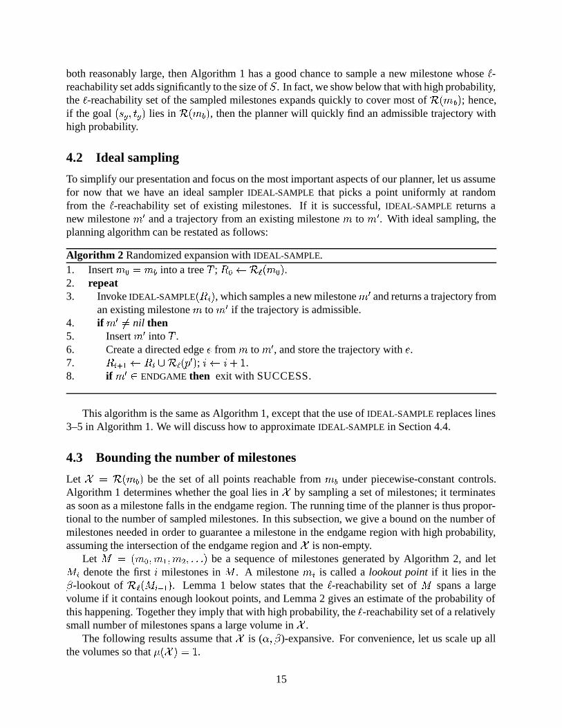
Thestandarddeviations in Table1 arelarger thanwhatwe would like. In Figure9, we showa histogramof morethan100 independentrunsfor a particularquery. In mostruns,the runningtime is well underthemeanor slightly above. This indicatesthatour plannerperformswell mostof thetime. Thelargedeviation is causedby a few runsthat take aslong asfour timesthemean.Thelongandthin tail of thedistribution is typicalof theteststhatwehaveperformed.

6 Air -cushionedrobots

6.1 Robot description

Ouralgorithmhasalsobeenimplementedandevaluatedonasecondsystem, whichwasdevelopedat the StanfordAerospaceRoboticsLaboratoryfor testingspaceroboticstechnology. This air-cushionedrobot (Figure1) movesfrictionlessly on a flat granitetableamongmoving obstacles.Eight air thrustersprovidesomni-directionalmotion capability, but the thrustavailable is smallcomparedto therobot’smass,resulting in tight accelerationconstraints.

Wedefinethestateof therobotto be �sVX�]Yp� �VX� �Y;� , where �WVX�]YD� arethecoordinatesof therobot’s

22

0 1 2 3 4 50

5

10

15

20

25

30

35

running time (seconds)

Figure9: Histogramof planningtimesfor morethan100runson a particularquery. Theaveragetime is 1.4sec,andthefour quartilesare0.6,1.1,1.9,and4.9seconds.

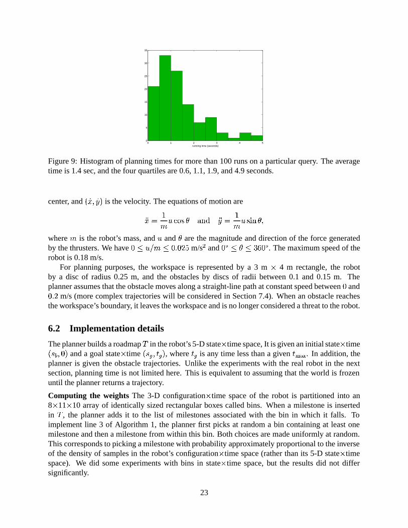
center, and � �VX� �Y;� is thevelocity. Theequationsof motionare

OV�� 8�� f>h9i \ alcZö OY�� 8

���i�j c \ �

where � is therobot’s mass,and � and \ arethemagnitudeanddirectionof the forcegeneratedby thethrusters.Wehave 5 , �pd �E, 5;<Ì5�:cg m/st and 5lk ,Ü\ , i d 5lk . Themaximumspeedof therobotis 0.18m/s.

For planningpurposes,the workspaceis representedby a 3 m � 4 m rectangle,the robotby a disc of radius0.25 m, and the obstaclesby discsof radii between0.1 and 0.15 m. Theplannerassumesthattheobstaclemovesalongastraight-linepathatconstantspeedbetween5 and5D<Ì: m/s(morecomplex trajectorieswill beconsideredin Section7.4). Whenanobstaclereachestheworkspace’sboundary, it leavestheworkspaceandis nolongerconsideredathreatto therobot.

6.2 Implementation details

Theplannerbuildsaroadmap� in therobot’s5-Dstate� timespace,It isgivenaninitial state� time�@�=�]�]5�� anda goalstate� time ���M�M�����?� , where ��� is any time lessthana given � ²X³@´ . In addition, theplanneris given the obstacletrajectories.Unlike the experimentswith the real robot in the nextsection,planningtime is not limited here.This is equivalentto assumingthat theworld is frozenuntil theplannerreturnsa trajectory.

Computing the weights The 3-D configuration� time spaceof the robot is partitioned into an8 � 11 � 10 arrayof identicallysizedrectangularboxescalledbins. Whena milestoneis insertedin � , the planneraddsit to the list of milestonesassociatedwith the bin in which it falls. Toimplement line 3 of Algorithm 1, the plannerfirst picks at randoma bin containingat leastonemilestoneandthenamilestonefrom within this bin. Bothchoicesaremadeuniformly at random.Thiscorrespondsto pickingamilestonewith probability approximatelyproportional to theinverseof thedensityof samplesin therobot’s configuration� time space(ratherthanits 5-D state� timespace). We did someexperimentswith bins in state� time space,but the resultsdid not differsignificantly.

23

Scene Time(sec) mov w pmean std mean std{}|B~0.249 0.264 2008 2229{��?~0.270 0.285 1946 2134{}�&~0.002 0.005 22 25

Table2: Performancestatisticsof theplanneron theair-cushionedrobot.

Implementing PROPAGATE Thesimplicity of theequationsof motion makesit possible to com-putetrajectoriesanalytically. Thetrajectoriesarethendiscretized,andateachdiscretizedstate� timepoint, the robot is checked for collision againstevery obstacle.This naive techniqueworks rea-sonablywell whenthenumberof obstaclesis small,but canbeeasilyimprovedto handlea largenumberof obstacles.

Endgame region The endgameregion is generatedwith specializedcurves, specifically, third-ordersplines.Wheneveranew milestone � is addedto � , it is checkedfor connectionwith 0 goalpoints ���A�M�����?� , for somepre-definedconstant0 . Eachof the 0 valuesof ��� is chosenuniformly atrandomfrom theinterval ~ � ²[Z]\ ��� ²X³@´ � , where� ²[Z]\ is anestimateof theearliesttime whentherobotmayreach �>� , given its maximum velocity. For eachvalueof �]� , theplannercomputesthe third-ordersplinebetween� and �@�=�M�����?� . It thenverifiesthatthespline is collision freeandsatisfiesthevelocityandaccelerationbounds.If all thetestssucceed,then � lies in theendgameregion. In alltheexperiments reportedbelow, 0 is setto 10.

6.3 Experimental results

We performedexperimentsin morethanonehundredsimulated environments. To simplify thesimulation, collisions amongobstaclesare ignored. So two obstaclesmay overlap temporarilywithout changingcourses.In a smallnumberof queries,theplannerfailed to returna trajectory,but in noneof thesecaseswerewe able to determinewhetheran admissible trajectoryactuallyexisted. On theotherhand,theplannersuccessfullysolvedseveralqueriesfor which we initiallythoughttherewasnosolution.

Threeexamplescomputedby the plannerare shown in Figure 10. For eachexample,wedisplayfive snapshots labeledby time. The largegraydisc indicatestherobot; thesmallerblackdiscsindicatetheobstacles.Thesolid anddottedlinesmark the trajectoriesof therobotandtheobstacles,respectively. For eachof thethreequeries,we rantheplanner100timesindependentlywith differentrandomseeds.Theplannersuccessfullyreturnedatrajectoryin all runs.Table2 liststhe meansandstandarddeviationsof the planningtimesandthe numberof sampledmilestonesfor eachquery. The reportedtimeswereobtainedfrom a plannerwritten in C andrunningon aPentium-IIIPCwith a550Mhz processorand128MB of memory.

In the first two examples,the moving obstaclescreatenarrow passagesthroughwhich therobotmustpassin orderto reachthegoal.Yetplanning timeremainsmuchunderonesecond.Thefact that theplannernever failed in 100 runstestifiesto its reliability. To point out thedifficultyof thesequeries,we show in Figure 11 the configuration� time spacefor example ���F� . In theconfiguration� time space,the robot mapsto a point �sVX�]Y^����� . Sincethe obstaclesare assumed

24

T = 0.0 secs T = 11.2 secs T = 22.4 secs T = 33.7 secs T = 44.9 secs

��WJ�T = 0.0 secs T = 9.0 secs T = 20.0 secs T = 30.0 secs T = 39.2 secs

���F�

T = 0.0 secs T = 8.0 secs T = 16.1 secs T = 24.1 secs T = 32.1 secs

� ¯ �Figure10: Computedexamplesfor theair-cushionedrobot.

to move with constantlinear velocity, they map into cylinders. The velocity and accelerationconstraintsrequireeverysolution trajectoryto passthroughasmallgapbetweenthecylinders.

Example � ¯ � is muchsimpler. Therearetwo stationaryobstaclesobstructing themiddle of theworkspaceandthreemoving obstacles.Planningtime is well below 0.01second,with anaverageof 0.002second.Thenumberof milestonesis alsosmall,confirmingtheresultof Theorem1 thatwhenthespaceis expansive,Algorithm1 is veryefficient. As in theexperimentsonnonholonomicrobot carts,the runningtime distribution of the plannertendsto have a long andthin tail duetolongexecutiontime in asmallnumberof runs,but overall theplanneris very fast.

25

��;� �l�

Figure11: Configuration� spacefor theexamplein Figure10� .

7 Experimentswith the real robot

To furthertesttheperformanceof theplanner, we connectedtheplannerdescribedin theprevioussectionto the air-cushionedrobot in Figure1. In thesetests,we examinedthe behavior of Al-gorithm1 runningin real-timemodeon a systemintegrating controlandsensingmodulesover adistributedarchitectureandoperatingin aphysicalenvironmentwith uncertaintiesandtimedelays.

7.1 Testbeddescription

Therobotshown in Figure1 is untetheredandmovesfrictionlessly onanair bearingona3 m � 4 mtable. Gastanksprovide compressedair for both theair-bearingandthrusters.An onboardMo-torola ppc2604computer performsmotion control at 60 Hz. Obstaclesarealsoon air-bearings,but have no thrusters.They areinitially propelledby handfrom variouslocationsandthenmovefrictionlessly on the tableat roughly constantspeeduntil they reachthe boundaryof the table,wherethey stopdueto thelackof air bearing.

An overheadvision systemestimatesthepositionsof therobotandtheobstaclesat 60 Hz bydetectingLEDs placedon the moving objects. The measurementis accurateto 5 mm. Velocityestimatesarederivedfrom position data.

Our plannerrunsoffboardon a 333Mhz SunSparc10. Theplanner, therobot,andthevisionmodulecommunicateover theradioEthernet.

7.2 Systemintegration

Implementing theplanneron thehardwaretestbedraisesseveralnew challenges.

Time delaysVariouscomputationsanddataexchangesoccurringat differentpartsof thesystemleadto delaysbetweenthe instantwhenthevision modulemeasuresthemotion of the robotandtheobstaclesandtheinstantwhentherobotstartsexecutingtheplannedtrajectory. Thesedelays,

26

if ignored,would causethe robot to begin executingtheplannedtrajectorybehindthestarttimeassumedby theplanner. The robotmaynot thenbe ableto catchup with theplannedtrajectorybeforea collisionoccurs.To dealwith this issue,theplannercomputesa trajectoryassuming thattherobotwill startexecutingit 0.4secondinto thefuture.It alsoassumesthattheobstaclesmoveatconstantvelocities,asmeasuredby thevision module,andextrapolatestheirpositionsaccordingly.The0.4 secondincludesall thedelaysin thesystem,in particular, the time neededfor planning.This time couldbefurtherreducedby implementingtheplannermorecarefullyandrunningit onamachinefasterthantherelatively slow SunSparc10currentlybeingused.

Sensingerrors Althoughtheplannerassumesthattheobstaclesmove alongstraightlinesat con-stantvelocitiesmeasuredby the vision module, the actualtrajectoriesareslightly differentdueto asymmetryin air-bearingsandinaccuracy in the measurements.The plannerdealswith theseerrorsby growing theobstacles.As time elapses,theradiusof eachmoving obstacleis increasedby ��� � , where � is a fixedconstant,� is themeasuredvelocity of theobstacle,and � is thetime.Sotheplannercanavoid erroneouslyassertingthata state� time point is collision-freewhenit isactuallynot.

Trajectory tracking The robot receivesfrom theplannera trajectorythat specifiesthe position,velocity, andacceleration of the robot at all times. A PD-controllerwith feedforward is usedtotrack this trajectory. The maximumtrackingerrorsfor the position andvelocity are0.05m and0.02m/s,respectively. As a result,we increasethesizeof thediscmodeling therobotby 0.05mduringtheplanningto guaranteethatthecomputedtrajectoryis collision-free.

Trajectory optimization Sincethe planneris very efficient in general,the 0.4 secondallocatedis often morethanwhat is neededfor finding a first solution. So the plannerexploits the extratime to generateadditionalmilestonesandkeepstrackof thebesttrajectoryfoundsofar. Thecostfunction for comparingtrajectoriesis �LI2 ( � �q� 2 �ð�F� ± 2 , where 0 is the numberof segmentsin thetrajectory, � 2 is the magnitudeof the force exertedby the thrustersalongthe 7 th segment, � is afixedconstant,and ± 2 is thedurationof the 7 th segment.Thecostfunctiontakesinto accountbothfuel consumption andexecution time. A larger � yieldsfastermotion, while asmaller� yieldslessfuel consumption. In ourexperiments, thecostof trajectorieswasreduced,ontheaverage,by 14%with thissimple improvement.

Safe-modeplanning If theplannerfailstofind atrajectoryto thegoalwithin theallocatedtime,wefoundit usefulto computeanescapetrajectory. Theendgameregion G������ for theescapetrajectoryconsistsof all the reachable,collision-freestates�@���F���?��� with �&��þ ������� for sometime ������� . Anescapetrajectorycorrespondsto any acceleration-bounded,collision-freemotionin theworkspacefor a smalldurationof time. In general,G������ is very large,andsogeneratinganescapetrajectoryoftentakeslittl etime. To ensurecollision-freemotionbeyond �S����� , anew escapetrajectorymustbecomputedlongbeforetheendof thecurrentescapetrajectorysothattherobotcanescapecollisiondespitetheacceleration constraints.Wemodifiedtheplannerto computesimultaneouslyanormalandanescapetrajectory. Themodificationincreasedtherunningtime of theplannerby about2%in ourexperiments,but it leadsto asystemthatis muchmoreusefulpractically.

27

Figure12: Snapshotsof therobotexecutinga trajectory.

7.3 Experimental results

Theplannersuccessfullyproducedcomplex maneuversof therobotamongstaticandmoving ob-staclesin varioussituations, includingobstaclesmoving directly towardtherobotor perpendicularto the line connectingits initial andgoalpositions. The testsalsodemonstratedtheability of thesystemto wait for anopeningto occurwhenconfrontedwith moving obstaclesin therobot’s de-sireddirectionof movement and to passthroughopeningsthat are lessthan10 cm larger thantherobot. In almostall thetrials, a trajectorywascomputedwithin theallocatedtime. Figure12shows snapshots of therobotduringoneof the trials, in which therobotmaneuversamongthreeincomingobstaclesto reachthegoalat thefront cornerof thetable.

Severalproblemslimited thecomplexity of theplanningproblemswhich we couldtry in thistestbed.Two arerelatedto the testbeditself. First the accelerationsprovided by the robot’s airthrustersarequite limited. Secondthesizeof the tableis small relative thatof therobotandtheobstacles,which limits the availablespacefor the robot to maneuver. The third problemresultsfrom thedesignof oursystem. Theplannerassumesthatobstaclesmoveat constantlinearveloci-tiesanddonotcollidewith oneother, anassumptionwhich is likely to fail in practice.To addressthis lastandimportantissue,we introduceon-the-flyreplanning.

7.4 On-the-fly replanning

An obstaclemaydeviatefrom its predictedtrajectory, becauseeithertheerrorin themeasurementsis larger thanexpected,or theobstacle’s directionof motionhassuddenly changeddueto a col-lision with otherobstacles.Whenever the vision module detectsthis, it alertsthe planner. Theplannerthenrecomputesa trajectoryon thefly within thesameallocatedtime limit , by projectingthestateof theworld 0.4secondinto thefuture.On-the-flyreplanningallowsmuchmorecomplex

28

−1 0 1

−1.5

−1

−0.5

0

0.5

1

1.5

T = 2.1 secs

x1 [meters]

x 2 [met

ers]

−1 0 1

−1.5

−1

−0.5

0

0.5

1

1.5

T = 14.6 secs

x1 [meters]

x 2 [met

ers]

−1 0 1

−1.5

−1

−0.5

0

0.5

1

1.5

T = 19.8 secs

x1 [meters]

x 2 [met

ers]

−1 0 1

−1.5

−1

−0.5

0

0.5

1

1.5

T = 33.2 secs

x1 [meters]

x 2 [met

ers]

−1 0 1

−1.5

−1

−0.5

0

0.5

1

1.5

T = 50.2 secs

x1 [meters]

x 2 [met

ers]

−1 0 1

−1.5

−1

−0.5

0

0.5

1

1.5

T = 75.0 secs

x1 [meters]

x 2 [met

ers]

Figure13: A computedexamplewith replanningin asimulatedenvironment.

experimentsto beperformed.Weshow two examplesbelow, onein simulationandoneon therealrobot.

In theexampleshows in Figure13,eightreplanningoperationsoccurredover theentirecourse(75seconds)of theexperiment.Initially therobotmovesto theleft to reachthegoalat thebottommiddle(snapshot1). Thentheupper-left obstaclechangesits motionandblockstherobot’s way,resultingin a replan(snapshot2). Soonafter, themotionof theupper-right obstaclealsochanges,forcingtherobotto reversethedirectionandapproachthegoalfromtheothersideof theworkspace(snapshot3). In theremainingtime,new changesin obstaclemotioncausetherobotto pause(seethesharpturn in snapshot5) until adirectapproachto thegoalis possible (snapshot6).

The efficacy of the replanningprocedureon the real robot is demonstratedby the examplein Figure 14. The robot’s goal is to move from the back left of the table to the front middle.Initially the obstaclein the middle is stationary, andthe other two obstaclesaremoving towardthe robot (snapshot1). The robot dodgesthe faster-moving obstaclefrom the left andproceedstowardthegoal(snapshot2). Theobstacleis thenredirectedtwice (in snapshots 3 and5) to blockthetrajectoryof therobot,causingit to slow down andstaybehindtheobstacleto avoid collision(snapshots3–6).Rightbeforesnapshot7, therightmost obstacleis directedbacktowardtherobot.Therobotwaitsfor theobstacleto pass(snapshot8) andfinally attainsthegoal(snapshot9). Theentiremotionlastsabout40seconds.Throughout thisexperiment, otherreplanningoperations(notshown) occurredasa resultof errorsin themeasurementof theobstaclemotions. However, noneresultedin amajorredirectionof therobot.

29

Figure14: An example with therealrobotusingon-the-flyreplanning.

8 Conclusion

Wehavepresentedasimple,efficient randomizedplannerfor kinodynamicmotionplanning in thepresenceof moving obstacles.Our algorithmrepresentsthemotionconstraintsby anequationoftheform

��S�°���@�9�]�p� andconstructsa roadmapof sampledmilestonesin thestate� time spaceofa robot. It samplesnew milestonesby first picking at randoma point in thespaceof admissiblecontrol functionsandthenmappingthe point into thestatespaceby integratingthe equationsofmotion. Thusthemotionconstraintsarenaturallyenforcedduringtheconstructionof theroadmap.Thealgorithmis generalandcanbeappliedto awideclassof systems,includingonesthatarenotlocally controllable.Theperformanceof thealgorithmhasbeenevaluatedthroughboththeoreticalanalysisandextensiveexperiments.

We have generalizedthe notion of expansiveness,originally proposedin [HLM97] for (geo-metric) pathplanning. The main purposeof the generalizationis to addressthe complicationsintroducedby kinematicanddynamicconstraints.Using the expansivenessto characterizethecomplexity of thestate� space,we have proven that,undersuitable assumptions,thefailureprob-

30

ability of theplannerconvergeto 0 at anexponential rate,whena solution exists. This resultalsoholdsfor robotsthatarenot locally controllable.

Experimentallythe plannerhasdemonstratedits effectivenessboth in simulation and on areal robot. Theexperimentson thereal robot indicatesthat theplannerworkswell despitemanyadversarialconditions, including (i) severedynamicconstraintson the motion of the robot, (ii)moving obstacles,and(iii) varioustime delaysanduncertaintiesinherentto an integratedsystemoperatingin a physical environment. In particular, they demonstratethat the efficiency of theplannerenablesit to beusedin realtimewhenobstaclestrajectoriesarenotknown in advance.

In thefuture,we planto apply theplannerto environmentswith morecomplex geometryandrobotswith higherdofs. Geometricalcomplexity increasesthe costof collision checking,but asdiscussedin Section2.4, hierarchicalalgorithmscandealwith this issueeffectively. In fact, asimilar, but simplerplannerhasbeenusedsuccessfullyto computegeometricdisassembly pathswith CAD modelshaving up to 200,000triangles[HLM99] .

We arealsointerestedin reducingthestandarddeviationof runningtimesfor our randomizedplanner. Quitepossibly, the thin andlong tail of the runningtime distribution shown in Figure9is typical of all PRM plannersdeveloped so far. However, it is more important to reduceit forsingle-queryplanners,becausethey are intendedto be usedinteractively or in real time. Largestandarddeviationsin thesesettingsareclearlyundesirable.

More importantly, we needto further develop tools to analyzethe efficiency of randomizedmotionplanners.Thenotionof expansivenessis astepforwardin thatdirection.However, thepa-rameterscharacterizinganexpansivespacecannotbeeasilydetermined,andsowecannotdecide,in advance,thenumberof milestonesneededfor agiven query. It is importantto continuelookingfor new analysistools; if we cannotmeasurethe performanceof thesealgorithms quantitatively,wewill notbeableto compare,improve, andthusadvanceourunderstandingof them.

Acknowledgments: This work wassupportedby ARO MURI grantDAAH04-96-1-007, NASA TRIWGCoop-AgreementNCC2-333,Real-TimeInnovations,andtheNIST ATPprogram.David Hsuhasalsobeenthe recipient of a Microsoft Graduate Fellowship, and RobertKindel, the recipient of an NSF GraduateFellowship.

References

[ABD 98] N.M. Amato, O.B. Bayazit, L.K. Dale, C. Jones,and D. Vallejo. OBPRM: Anobstacle-basedPRMfor 3Dworkspaces.In P.K. Agarwaletal.,editors,Robotics: TheAlgorithmicPerspective:1998WorkshopontheAlgorithmicFoundationsofRobotics,pages155–168.A. K. Peters,Wellesley, MA, 1998.

[AG99] J.M. AhuactzinandK.K. Gupta. Thekinematicroadmap:A motionplanningbasedglobal approachfor inversekinematics of redundantrobots. IEEE TransactionsonRoboticsandAutomation, 15(4):653–669,1999.

[Aga97] P.K. Agawal. Rangesearching.In J.E.GoodmanandJ.O’Rourke,editors,Handbookof discreteandcomputational geometry, pages575–598. CRCPress,BocaRaton,FL,1997.

31

[Ahu94] J.M. Ahuactzin. Le Fil d’Ariane. Une methodede planification general. Applica-tion a la planfification destrajectoires. PhDthesis,NationalPolytechnicInstitute ofGrenoble,France,1994.

[BDG85] J.E. Bobrow, S.Dubowsky, andJ.S.Gibson. Time-optimalcontrolof roboticmanip-ulatorsalongspecifiedpaths.InternationalJournalof RoboticsResearch, 4(3):3–17,1985.

[BK00] R. Bohlin andL.E. Kavraki. PathplanningusinglazyPRM. In Proc.IEEEInt. Conf.onRoboticsandAutomation, 2000.

[BKL 97] J. Barraquand,L. Kavraki, J.C. Latombe,T.-Y. Li, R. Motwani, andP. Raghavan.A randomsamplingschemefor path planning. International Journal of RoboticsResearch, 16(6):759–774,1997.

[BL89] J.BarraquandandJ.C.Latombe.Onnonholonomic robotsandoptimalmaneuvering.Revued’IntelligenceArtificielle, 3(2):77–103,1989.

[BL91] J.BarraquandandJ.C.Latombe.Robotmotionplanning:A distributedrepresentationapproach.International Journal of RoboticsResearch, 10(6):628–649,1991.

[BL93] J. BarraquandandJ.C.Latombe.Nonholonomicmultibodymobilerobots:Control-lability andmotionplanningin thepresenceof obstacles.Algorithmica, 10(2-4):121–155,1993.

[BOvdS99] V. Boor, M.H. Overmars,andF. vanderStappen.Thegaussiansampling strategy forprobabilistic roadmapplanners.In Proc.IEEEInt. Conf. onRoboticsandAutomation,pages1018–1023, 1999.

[CL95] H. ChangandT.-Y. Li. Assembly maintainability studywith motion planning. InProc.IEEE Int. Conf. onRoboticsandAutomation, pages1012–1019,1995.

[CLMP95] J.Cohen,M. Lin, D. Manocha,andM. Ponamgi.I-Collide: An interactiveandexactcollisiondetectionsystemfor largescaleenvironments. In Proc.ACM Interactive3DGraphicsConf., pages189–196,1995.

[DK99] J.P. DesaiandV. Kumar. Motionplanningfor cooperatingmobilemanipulators.Jour-nal of Robotic Systems, 16(10):557–579,1999.

[Don87] B.R. Donald. A searchalgorithmfor motion planningwith six degreesof freedom.Artificial Intelligence, 31(3):295–353,1987.

[DXCR93] B.R.Donald,P. Xavier, J.Canny, andJ.Reif. Kinodynamic motionplanning.Journalof theACM, 40(5):1048–1066,1993.

[ELP86] M. ErdmannandT. Lozano-Perez. On multiple moving objects. In Proc. IEEE Int.Conf. onRoboticsandAutomation, pages1419–1424,1986.

32

[ELP87] M. Erdmannand T. Lozano-Perez. On multiple moving objects. Algorithmica,2(4):477–521, 1987.

[Fer98] P. Ferbach.A methodof progressive constraintsfor nonholonomicmotion planning.IEEETransactionsonRoboticsandAutomation, 14(1):172–179,1998.

[Fra93] T. Fraichard.Dynamictrajectoryplanning with dynamicconstraints:A “state-timespace”approach.In Proc. IEEE/RSJInternational Conferenceon IntelligentRobotsandSystems, volume2, pages1394–1400, 1993.

[FS96] P. Fiorini andZ. Shiller. Time optimal trajectoryplanningin dynamic environments.In Proc.IEEE Int. Conf. onRoboticsandAutomation, pages1553–1558,1996.

[Fuj95] K. Fujimura. Time-minimumroutesin time-dependentnetworks. IEEETransactionsonRoboticsandAutomation, 11(3):343–351,1995.

[GLM96] S.Gottschalk,M. Lin, andD. Manocha.OBB-Tree:A hierarchicalstructurefor rapidinterferencedetection. In SIGGRAPH96 ConferenceProceedings, pages171–180,1996.

[HK77] R.HermannandA.J.Krener. Nonlinearcontrollability andobservability. IEEETrans-actionsonAutomaticControl, 22(5):728–740, 1977.

[HKL 98] D. Hsu, L. Kavraki, J.C. Latombe,R. Motwani, and S. Sorkin. On finding nar-row passageswith probabilistic roadmapplanners. In P.K. Agarwal et al., editors,Robotics:TheAlgorithmicPerspective:1998Workshopon theAlgorithmic Founda-tionsof Robotics, pages141–154.A. K. Peters,Wellesley, MA, 1998.

[HKLR00] D. Hsu, R. Kindel, J.C.Latombe,andS. Rock. Randomizedkinodynamic motionplanningwith moving obstacles. In B.R. Donald et al., editors,Algorithmic andComputational Robotics: New Directions:TheFourthInternational WorkshopontheAlgorithmicFoundationsof Robotics, pages247–264.A. K. Peters,Wellesley, MA,2000.

[HLM97] D. Hsu, J.C.Latombe,andR. Motwani. Path planningin expansive configurationspaces. In Proc. IEEE Int. Conf. on Roboticsand Automation, pages2719–2726,1997.

[HLM99] D. Hsu, J.C.Latombe,andR. Motwani. Path planningin expansive configurationspaces. International Journal of Computational Geometry& Applications, 9(4 &5):495–512, 1999.

[HLMK99] D. Hsu,J.C.Latombe,R. Motwani,andL.E. Kavraki. Capturingtheconnectivity ofhigh-dimensionalgeometricspacesby parallelizablerandomsamplingtechniques.InP.M. PardalosandS.Rajasekaran,editors,Advancesin randomizedparallel comput-ing, pages159–182.Kluwer AcademicPublishers,Boston,MA, 1999.

33

[HST94] T. Horsch,F. Schwarz,andH. Tolle. Motion planningfor many degreesof freedom— randomreflectionsatC-Spaceobstacles.In Proc.IEEEInt. Conf. onRoboticsandAutomation, pages3318–3323,1994.

[Hsu00] D. Hsu.RandomizedSingle-queryMotionPlanning in ExpansiveSpaces. PhDthesis,Dept.of ComputerScience,StanfordUniversity, Stanford,CA, May 2000.

[Hub96] P.M. Hubbard.Approximating polyhedrawith spheresfor time-criticalcollision de-tection.ACM TransactionsonGraphics, 15(3):179–210, 1996.

[HXCW98] Y.K. Hwang, P.G. Xavier, P.C. Chen,andP.A. Watterberg. Motion planningwithSANDROS andthe configurationspacetoolkit. In K.K. GuptaandA.P. del Pobil,editors,Practical Motion Planningin Robotics, pages55–77.JohnWiley & Sons,1998.

[Kav94] L.E. Kavraki. RandomNetworksin Configuration Spacefor Fast Path Planning.PhDthesis,Dept.of ComputerScience,StanfordUniverity, Stanford,CA, December1994.

[KHLR00] R. Kindel,D. Hsu,J.C.Latombe,andS.Rock.Kinodynamicmotionplanningamidstmovingobstacles.In Proc.IEEE Int. Conf. onRoboticsandAutomation, pages537–543,2000.

[KHM 98] J. Klosowski, M. Held, J.S.B.Mitchell, H. Sowizral, andK. Zikan. Efficient colli-siondetectionusingbounding volume hierarchiesof k-dops. IEEE TransactionsonVisualizationandComputerGraphics, 4(1):21–37,1998.

[Kin01] R. Kindel. Motion Planningfor Free-FlyingRobotsin DynamicandUncertainEn-vironments. PhD thesis,Dept.of Aeronautics& Astronautics, StanfordUniversity,Stanford,CA, October2001.

[KKL98] L. Kavraki, M.N. Kolountzakis, and J.C. Latombe. Analysis of probabilisticroadmapsfor path planning. IEEE Transactionson Robotics and Automation,14(1):166–171, 1998.

[KLMR95] L. Kavraki, J.C.Latombe,R.Motwani,andP. Raghavan.Randomizedqueryprocess-ing in robotpathplanning.In Proc.ACM SymposiumonTheoryof Computing, pages353–362,1995.

[KPLM98] S. Krishnan,A. Pattekar, M. Lin, andD. Manocha.Sphericalshell: A higherorderboundingvolume for fastproximity queries.In Robotics:TheAlgorithmicPerspec-tive: 1998Workshopon the Algorithmic Foundations of Robotics, pages177–190,1998.

[KSLO96] L. Kavraki, P. Svestka,J.C.Latombe,andM.H. Overmars. Probabilistic roadmapsfor pathplanning in high-dimensional configurationspace. IEEE TransactionsonRoboticsandAutomation, 12(4):566–580,1996.

34

[Kuf99] J.J.Kuffner. AutonomousAgentsfor Real-Time Animation. PhD thesis,Dept. ofComputerScience,StanfordUniversity, Stanford,CA, December1999.

[KW86] M.H. KalosandP.A. Whitlock. MonteCarlo Methods, volume1. JohnWiley & Son,New York, 1986.

[KZ86] K. Kant andS.W. Zucker. Toward efficient trajectoryplanning: The path-velocitydecomposition. InternationalJournalof RoboticsResearch, 5(3):72–89,1986.

[Lat99] J.C.Latombe.Motion planning: A journey of robots,molecules,digital actors,andotherartifacts.InternationalJournalof RoboticsResearch, 18(11):1119–1128,1999.

[Lau86] J.-P. Laumond. Feasibletrajectoriesfor mobile robotswith kinematicandenviron-mentalconstraints. In Proc. Int. Conf. on Intelligent Autonomous Systems, pages346–354,1986.

[LCH89] Z. Li, J.F. Canny, andG. Heinzinger. Robotmotion planningwith nonholonomicconstraints.In H. Miura et al., editors,Robotics Research: TheFifth InternationalSymposium, pages309–316.MIT Press,Cambridge,MA, 1989.

[LH00] P. Leven andS. Hutchinson. Toward real-timepathplanningin changingenviron-ments.In B.R. Donaldet al., editors,Algorithmic andComputational Robotics: NewDirections: TheFourth International Workshopon the Algorithmic FoundationsofRobotics, pages363–376.A. K. Peters,Wellesley, MA, 2000.

[LJTM94] J.-P. Laumond,P.E. Jacobs.,M. Taıx., and R.M. Murray. A motion plannerfornonholonomic mobile robots. IEEE Transactions on Roboticsand Automation,10(5):577–593, 1994.

[LK99] S.M. LaValle andJ.J.Kuffner. Randomizedkinodynamic planning. In Proc. IEEEInt. Conf. onRoboticsandAutomation, pages473–479, 1999.

[LK01] S.M. LaValle andJ.J.Kuffner. Randomizedkinodynamic planning. InternationalJournalof RoboticsResearch, 20(5):278–400,May 2001.

[LL96] F. LamirauxandJ.-P. Laumond. On theexpectedcomplexity of randompathplan-ning. In Proc.IEEEInt. Conf. onRoboticsandAutomation, pages3014–3019, 1996.

[LM96] K.M. LynchandM.T. Mason. Stablepushing: Mechanics,controllability, andplan-ning. International Journal of RoboticsResearch, 15(6):533–556,1996.

[O’R97] J. O’Rourke. Visibility. In J.E.GoodmanandJ. O’Rourke, editors,Handbookofdiscreteandcomputational geometry, pages467–479. CRC Press,BocaRaton,FL,1997.

[PTVP92] W.H. Press,S.A. Teukolsky, W.T. Vetterling,andB.P. Plannery. NumericalRecipesin C. CambridgeUniversity Press,2ndedition,1992.

35

[Qui94] S. Quinlan. Efficient distancecomputation betweennon-convex objects. In Proc.IEEE Int. Conf. onRoboticsandAutomation, pages3324–3329,1994.

[Rei79] J.H. Reif. Complexity of the mover’s problemandgeneralizations.In Proc. IEEESymposiumonFoundationsof ComputerScience, pages421–427,1979.

[RS85] J.H. Reif andM. Sharir. Motion planningin the presenceof moving obstacles.InProc.IEEESymposiumonFoundationsof ComputerScience, pages144–154,1985.

[RS90] J.A.ReedsandL.A. Shepp.Optimalpathsfor acarthatgoesforwardsandbackwards.PacificJournal of Mathematics, 145(2):367–393,1990.

[SA01] G. Sanchez-Ante.Single-QueryBi-DirectionalMotionPlanningwith LazyCollisionChecking. PhDthesis,ITESM, CampusCuernavaca,Mexico, 2001.

[SD91] Z. ShillerandS.Dubowsky. Oncomputing theglobaltime-optimal motionsof roboticmanipulators in the presenceof obstacles.IEEE Transactionson Roboticsand Au-tomation, 7(6):785–797,1991.

[SL98] S.SekhavatandJ.-P. Laumond. Topologicalpropertyfor collision-freenonholonomicmotion planning: The caseof sinusoidal inputs for chainedform systems. IEEETransactionsonRoboticsandAutomation, 14(5):671–680,1998.

[SLL01] T. Simeon,J.P. Laumond, andF. Lamiraux.Move3D:A genericplatformfor motionplanning. In Proc. IEEE International Symposiumon AssemblyandTaskPlanning,2001.

[SMA01] G. Song,S. Miller, andN. Amato. Customizing PRM roadmapsat querytime. InProc.IEEE Int. Conf. onRoboticsandAutomation, 2001.

[SO94] P. SvestkaandM.H. Overmars. Motion planningfor car-like robotsusinga prob-abilistic learningapproach. TechnicalReportRUU-CS-94-33, Dept. of ComputerScience,UtrechtUniversity, Utrecht,TheNetherlands,1994.

[SO98] P. SvestkaandM.H. Overmars.Probabilistic pathplanning:Robotmotionplanningandcontrol.In LectureNotesin Control andInformation Sciences, volume229,pages225–304.Springer-Verlag,1998.

[SSLO97] S. Sekhavat, P. Svestka,J.-P. Laumond,andM.H. Overmars.Multi-level pathplan-ning for nonholonomic robotsusingsemi-holonomicsubsystems. In J.-P. Laumondet al., editors,Algorithmsfor RoboticMotion andManipulation: 1996WorkshopontheAlgorithmic Foundationsof Robotics, pages79–96.A. K. Peters,Wellesley, MA,1997.

[Sve97] P. Svestka.RobotMotionPlanningUsingProbabilistic Roadmaps. PhDthesis,Dept.of ComputerScience,UtrechtUniversity, TheNetherland,1997.

36