randomized online pca algorithms with regret bounds that are
TRANSCRIPT

Journal of Machine Learning Research 9 (2008) 2287-2320 Submitted 9/07; Published 10/08
Randomized Online PCA Algorithms with Regret Bounds that areLogarithmic in the Dimension∗
Manfred K. Warmuth [email protected]
Dima Kuzmin [email protected]
Computer Science DepartmentUniversity of California - Santa CruzSanta Cruz, CA, 95064
Editor: John Shawe-Taylor
AbstractWe design an online algorithm for Principal Component Analysis. In each trial the current instanceis centered and projected into a probabilistically chosen low dimensional subspace. The regret ofour online algorithm, that is, the total expected quadratic compression loss of the online algorithmminus the total quadratic compression loss of the batch algorithm, is bounded by a term whosedependence on the dimension of the instances is only logarithmic.
We first develop our methodology in the expert setting of online learning by giving an algorithmfor learning as well as the best subset of experts of a certain size. This algorithm is then lifted tothe matrix setting where the subsets of experts correspond to subspaces. The algorithm representsthe uncertainty over the best subspace as a density matrix whose eigenvalues are bounded. Therunning time is O(n2) per trial, where n is the dimension of the instances.Keywords: principal component analysis, online learning, density matrix, expert setting, quantumBayes rule
1. Introduction
In Principal Component Analysis (PCA) the n-dimensional data instances are projected into a k-dimensional subspace (k < n) so that the total quadratic compression loss is minimized. Aftercentering the data, the problem is equivalent to finding the eigenvectors of the k largest eigenvaluesof the data covariance matrix. The variance along an eigendirection is always equal to the corre-sponding eigenvalue and the subspace defined by the eigenvectors corresponding to the k largesteigenvalues is the subspace that captures the largest total variance and this is equivalent to minimiz-ing the total quadratic compression loss.
We develop a probabilistic online version of PCA: in each trial the algorithm chooses a centermt−1 and a k-dimensional projection matrix Pt−1 based on some internal parameter (which summa-rizes the information obtained from the previous t −1 trials); then an instance xt is received and thealgorithm incurs compression loss ‖(xt −mt−1)−Pt−1(xt −mt−1)‖2
2; finally, the internal parametersare updated. The goal is to obtain online algorithms whose total compression loss in all trials is
close to the total compression loss minm,P
T
∑t=1
‖(xt −m)−P(xt −m)‖22 of the batch algorithm which can
choose its center and k-dimensional subspace in hindsight based on all T instances. Specifically,
∗. Supported by NSF grant IIS 0325363. A preliminary version of this paper appeared in Warmuth and Kuzmin (2006b).
c©2008 Manfred K. Warmuth and Dima Kuzmin.

WARMUTH AND KUZMIN
in this paper we obtain randomized online algorithms with bounded regret. Here we define regretas the difference between the total expected compression loss of the randomized online algorithmand the compression loss of the best mean and subspace of rank k chosen offline. In other wordsthe regret is essentially the expected additional compression loss incurred by the online algorithmcompared to normal batch PCA. The expectation is over the internal randomization of the algorithm.
We begin by developing our online PCA algorithm for the uncentered case, that is, all mt = 0 and
the compression loss of the offline comparator is simplified to minP
T
∑t=1
‖xt −Pxt‖22. In this simpler
case our algorithm is motivated by a related problem in the expert setting of online learning, whereour goal is to perform as well as the best size k subset of experts. The algorithm maintains a mixturevector over the n experts. At the beginning of trial t the algorithm chooses a subset Pt−1 of k expertsbased on the current mixture vector wt−1 that summarizes the previous t −1 trials. It then receives aloss vector `t ∈ [0,1]n. Now the subset Pt−1 corresponds to the subspace onto which we “compress”or “project” the data. The algorithm incurs no loss on the k components of Pt−1 and its compressionloss equals the sum of the remaining n− k components of the loss vector, that is, ∑i∈{1,...,n}−Pt−1 `t
i .Finally it updates its mixture vector to wt .
The key insight is to maintain a mixture vector wt−1 as a parameter with the additional constraintthat wt−1
i ≤ 1n−k . We will show that this “capped” mixture vector represents an implicit mixture
over all subsets of experts of size n − k, and given wt−1 we can efficiently sample a subset ofsize n− k from the implicit mixture and choose Pt−1 as the complementary subset of size k. Thisgives an online algorithm whose total loss over all trials is close to the smallest n− k componentsof the total loss vector ∑T
t=1 `t . We will show how this algorithm generalizes to an online PCAalgorithm when the mixture vector wt−1 is replaced by a density matrix W t−1 whose eigenvalues arecapped by 1
n−k . Now the constrained density matrix W t−1 represents an implicit mixture of (n− k)-dimensional subspaces. Again, we can efficiently sample from this mixture, and the complementaryk-dimensional subspace Pt−1 is used for projecting the current instance xt at trial t.
A simple way to construct an online algorithm is to run the offline or batch algorithm on alldata received so far and use the resulting hypothesis on the next data instance. This is called the“Incremental Offline Algorithm” (Azoury and Warmuth, 2001). When the offline algorithm justminimizes the loss on the past instances, then this algorithm is also called the “Follow the Leader(FL) Algorithm” (Kalai and Vempala, 2005). For uncentered PCA we can easily construct a se-quence of instances for which the total online compression loss of FL is n
n−k times larger than thetotal compression loss of batch PCA. However, in this paper we have a more stringent goal. Wedesign randomized online algorithms whose total expected compression loss is at most one timesthe compression loss of batch PCA plus an additional lower order term which we optimize. In otherwords, we are seeking online algorithms with bounded regret. Our regret bounds are worst-case inthat they hold for arbitrary sequences of instances.
Simple online algorithms such as the Generalized Hebbian Algorithm (Sanger, 1989) have beeninvestigated previously that provably converge to the best offline solution. No worst-case regretbounds have been proven for these algorithms. More recently, the online PCA problem was alsoaddressed in Crammer (2006). However, that paper does not fully capture the PCA problem becausethe presented algorithm uses a full-rank matrix as its hypothesis in each trial, whereas we use aprobabilistically chosen projection matrix of the desired rank k. Furthermore, that paper provesbounds on the filtering loss, which are typically easier to obtain, and it is not clear how the filteringloss relates to the more standard regret bounds for the compression loss proven in this paper.
2288

ONLINE PCA
Our algorithm is unique in that we can prove a regret bound for it that is linear in the tar-get dimension k of the subspace but logarithmic in the dimension of the instance space. The keymethodology is to use a density matrix as the parameter and employ the quantum relative entropy asa regularizer and measure of progress. This was first done in Tsuda et al. (2005) for a generalizationof linear regression to the case when the parameter matrix is a density matrix. Our update of thedensity matrix can be seen as a “soft” version of computing the top k eigenvectors and eigenvaluesof the covariance matrix. It involves matrix logarithms and exponentials which are seemingly morecomplicated than the FL Algorithm which simply picks the top k directions. Actually, the most ex-pensive step in both algorithms is to update the eigendecomposition of the covariance matrix aftereach new instance, and this costs O(n2) time (see, e.g., Gu and Eisenstat, 1994).
The paper is organized as follows. We begin by introducing some basics about batch and onlinePCA (Section 2) as well as the Hedge Algorithm from the expert setting of online learning (Section3). We then develop a version of this algorithm that learns as well as the best subset of expertsof fixed size (Section 4). When lifted to the matrix setting, this algorithm does uncentered PCAonline (Section 5). Surprisingly, the regret bound for the matrix setting stays the same and this isan example of a phenomenon that has been dubbed the “free matrix lunch” (Warmuth, 2007b). Webriefly discuss the merits of various alternate algorithms in sections 4.1 and 5.1.
Our online algorithm for centered online PCA is more involved since it has to learn the centeras well (Section 6). After motivating the updates to the parameters (Section 6.1) we generalizeour regret bound to the centered case (Section 6.2). We then briefly describe how to constructbatch PCA algorithms from our online algorithms via standard conversion techniques (Section 6.3).Surprisingly, the bounds obtained this way are competitive with the best known batch PCA bounds.Lower bounds are discussed in Section 7. A brief experimental evaluation is given in Section 8 andwe conclude with an overview of online algorithms for matrix parameters and discuss a number ofopen problems (Section 9).
2. Setup of Batch PCA and Online PCA
Given a set (or batch) of instance vectors {x1, . . . ,xT}, the goal of batch PCA is to find a low-dimensional approximation of this data that minimizes the quadratic compression loss. Specifically,we want to find a center vector m ∈ R
n and a rank k projection matrix1 P such that the followingloss function is minimized:
comp(P,m) =T
∑t=1
‖(xt −m)−P(xt −m)‖22. (1)
Differentiating and solving for m gives us m∗ = x, where x is the data mean. Substituting this optimalcenter m∗ into loss (1) we obtain
comp(P) =T
∑t=1
‖(I −P)(xt − x)‖22 =T
∑t=1
(xt − x)>(I −P)2(xt − x)
= tr((I −P)2
T
∑t=1
(xt − x)(xt − x)>
︸ ︷︷ ︸C
).
1. Projection matrices are symmetric matrices P with eigenvalues in {0,1}. Note that P2 = P.
2289

WARMUTH AND KUZMIN
The sum of outer products in the above trace is called the data covariance matrix C. Since I−P is aprojection matrix, (I −P)2 = I −P, and
comp(P) = tr(( I −P︸︷︷︸rank n−k
)C) = tr(C)− tr( P︸︷︷︸rank k
C).
We call the above loss the compression loss of P or the loss of subspace I −P. We now give ajustification for this choice of terminology. Observe that tr(C) equals tr(CP)+ tr(C(I−P)), the sumof the losses of the complementary subspaces. However, we project the data into subspace P andthe projected parts of the data are perfectly reconstructed. We charge the subspace P with the partsthat are missed, that is, tr((I −P)C), and therefore call this the compression loss of P.
We now show that tr(PC) is maximized (or tr((I − P)C) minimized) if P consists of the keigendirections of C with the largest eigenvalues. This proof might seem a digression, but ele-ments of it will appear throughout the paper. By rewriting C in terms of its eigendecomposition,that is, C = ∑n
i=1 γi cic>i , we can upper bound tr(PC) as follows:
tr(PC) =n
∑i=1
γi tr(P cic>i ) =
n
∑i=1
γi c>i Pci ≤ max0≤δi≤1,∑i δi=k
n
∑i=1
γi δi.
We can replace the scalars c>i Pci in the ending inequality by the constrained δi’s because of thefollowing facts:
c>i Pci ≤ 1, for 1 ≤ i ≤ n, andn
∑i=1
c>i Pci = tr(Pn
∑i=1
cic>i
︸ ︷︷ ︸I
) = tr(P) = k,
since the eigenvectors ci of C are an orthogonal set of n directions. A linear function is maximizedat one of the vertices of its polytope of feasible solutions. The vertices of this polytope defined bythe constraints 0 ≤ δi ≤ 1 and ∑i δi = k are those δ vectors with exactly k ones and n−k zeros. Thusthe vertices of the polytope correspond to sets of size k and
tr(PC) ≤ max1≤i1<i2<...<ik≤n
k
∑j=1
γi j .
Clearly the set that gives the maximum upper bound corresponds to the largest k eigenvalues of Cand tr(P∗C) equals the above upper bound when P∗ consists of the eigenvectors corresponding tothe set of k largest eigenvalues.
In the online setting, learning proceeds in trials. At trial t the algorithm chooses a center mt−1
and a rank k projection matrix Pt−1. It then receives an instance xt and incurs loss
‖(xt −mt−1)−Pt−1(xt −mt−1)‖22 = tr((I −Pt−1)(xt −mt−1)(xt −mt−1)>).
Note that this is the compression loss of the center mt−1 and subspace Pt−1 on the instance xt . Ourgoal is to obtain an algorithm whose total online compression loss over the entire sequence of Ttrials ∑T
t=1 tr((I−Pt−1)(xt −mt−1)(xt −mt−1)>) is close to the total compression loss (1) of the bestcenter m∗ and best rank k projection matrix P∗ chosen in hindsight by the batch algorithm.
2290

ONLINE PCA
3. Learning as Well as the Best Expert with the Hedge Algorithm
The following setup and algorithm will be the basis of this paper. The algorithm maintains a prob-ability distribution wt−1 over n experts. At the beginning of trial t it chooses an expert probabilis-tically according to the probability vector wt−1, that is, expert i is chosen with probability wt−1
i .Then a loss vector `t ∈ [0,1]n is received, where `t
i specifies the loss of expert i incurred in trial t.The expected loss of the algorithm will be wt−1 · `t , since the expert was chosen probabilistically.At the end of the trial, the probability distribution is updated to wt using exponential update factors(See Algorithm 1). This is essentially the Hedge Algorithm of Freund and Schapire (1997). In the
Algorithm 1 Hedge Algorithm
input: Initial n-dimensional probability vector w0
for t = 1 to T doDraw an expert i with probability wt−1
iReceive loss vector `t
Incur loss `ti
and expected loss wt−1 · `t
wti =
wt−1i exp(−η`t
i)
∑nj=1 wt−1
j exp(−η`tj)
end for
original version the algorithm proposes a distribution wt−1 at trial t and incurs loss wt−1 · `t (insteadof drawing an expert from wt−1 and incurring expected loss wt−1 · `t).
It is easy to prove the following bound on the total expected loss. Here d(u,w) denotes therelative entropy between two probability vectors d(u,w) = ∑n
i=1 ui log uiwi
and log is the natural log-arithm.
Theorem 1 For an arbitrary sequence of loss vectors `1, . . . , `T ∈ [0,1]n, the total expected loss ofAlgorithm 1 is bounded as follows:
T
∑t=1
wt−1 · `t ≤ η∑Tt=1 u · `t +
(d(u,w0)−d(u,wT )
)
1− exp(−η),
for any learning rate η > 0 and comparison vector u in the n dimensional probability simplex.
Proof The update for wt in Algorithm 1 is essentially the update of the Continuous WeightedMajority Algorithm where the absolute loss of expert i is replaced by `t
i . Since `ti ∈ [0,1], we
have exp(−η`ti)≤ 1− (1−exp(−η))`t
i and this implies (essentially Littlestone and Warmuth 1994,Lemma 5.2, or Freund and Schapire 1997):
− logn
∑i=1
wt−1i exp(−η`t
i) ≥− log(1− (1− exp(−η))wt−1 · `t)) ≥ wt−1 · `t(1− exp(−η)).
The above can be reexpressed with relative entropies as follows (Kivinen and Warmuth, 1999):
d(u,wt−1)−d(u,wt) = −ηu · `t − logn
∑i=1
wt−1i exp(−η`t
i)
≥ −ηu · `t +wt−1 · `t(1− exp(−η)). (2)
2291

WARMUTH AND KUZMIN
The bound of theorem can now be obtained by summing over trials.
The original Weighted Majority algorithms were described for the absolute loss (Littlestone andWarmuth, 1994). The idea of using loss vectors instead was introduced in Freund and Schapire(1997). The latter paper also shows that when ∑t u · `t ≤ L and d(u,w0)− d(u,wT ) ≤ D ≤ logn,then with η = log(1+
√2D/L), we get the bound
∑t
wt−1 · `t ≤ ∑t
u · `t +√
2LD+d(u,w0)−d(u,wT ). (3)
By setting u to be the vector with a single one identifying the best expert, we get the followingbound on the regret of the algorithm (Again log denotes the natural logarithm.):
total loss of alg. − total loss of best expert ≤√
2 (total loss of best expert) logn+ logn.
4. Learning as Well as the Best Subset of Experts
Recall that projection matrices are symmetric positive definite matrices with eigenvalues in {0,1}.Thus a rank k projection matrix can be written as P = ∑k
i=1 pi p>i , where the pi are the k orthonor-
mal vectors forming the basis of the subspace. Assume for the moment that the eigenvectors arerestricted to be standard basis vectors. Now a projection matrix becomes a diagonal matrix withk ones in the diagonal and n− k zeros. Also, the trace of a product of such a diagonal projectionmatrix and any symmetric matrix specifying the loss becomes a dot product between the diagonalsof both matrices. The diagonal of the symmetric matrix may be seen as a loss vector `t . Thus, inthis simplified diagonal setting, our goal is to develop online algorithms whose total loss is close tothe sum of the lowest n− k components of total loss vector ∑T
t=1 `t . Equivalently, we want to findthe highest k components of the total loss vector and per our nomenclature the loss of the lowestn− k components is the compression loss of the complementary highest k components.
For this problem, we will encode the subsets of size n− k as probability vectors: we call r ∈[0,1]n an (n−k)-corner if it has n−k components fixed to 1
n−k and the remaining k components fixedto zero. The algorithm maintains a probability vector wt as its parameter. At trial t it probabilisticallychooses an (n−k)-corner r based on the current probability vector wt−1 (Details of how this is donewill be given shortly). The set of k components missed by r is the set Pt−1 that we compress withat trial t. The algorithm then receives a loss vector `t and incurs compression loss (n− k)r · `t =
∑i∈{1,...,n}−Pt−1 `ti . Finally the weight vector wt−1 is updated to wt .
We now describe how the corner is chosen: The current probability vector is decomposed into amixture of n corners and then one of the n corners is chosen probabilistically based on the mixturecoefficients. In the description of the decomposition algorithm we use d = n−k for convenience. LetAn
d denote the convex hull of the(n
d
)corners of size d (where 1 ≤ d < n). Clearly, any component
wi of a vector w in the convex hull is at most 1d because it is a convex combination of numbers
in {0, 1d}. Therefore An
d ⊆ Bnd , where Bn
d is the capped probability simplex, that is, the set of n-dimensional vectors w for which |w| = ∑i wi = 1 and 0 ≤ wi ≤ 1
d , for all i. Figure 1 depicts thecapped probability simplex for case d = 2 and n = 3,4. The following theorem shows that theconvex hull of the corners is exactly the capped probability simplex, that is, An
d = Bnd . It shows this
by expressing any probability vector in the capped simplex Bnd as a convex combination of at most
n d−corners. For example, when d = 2 and n = 4, Bnd is an octahedron (which has 6 vertices).
However, each point in this octahedron is contained in a tetrahedron which is the hull of only 4 ofthe 6 total vertices.
2292

ONLINE PCA
Figure 1: The capped probability simplex Bnd , for d = 2 and n = 3,4. This simplex is the intersection
of n halfspaces (one per capped dimension) and its vertices are the(n
d
)d-corners.
Figure 2: A step of the Mixture Decomposition Algorithm 2, n = 6 and k = 3. When a corner isremoved, then at least one more component is set to zero or raised to a d-th fraction of thetotal weight. The left picture shows the case where a component inside the corner gets setto zero and the right one depicts the case where a component outside the picked cornergets d-th fraction of the total weight.
Theorem 2 Algorithm 2 decomposes any probability vector w in the capped probability simplex Bnd
into a convex combination2 of at most n d-corners.
Proof Let b(w) be the number of boundary components in w, that is, b(w)= |{i : wi is 0 or |w|d }|.
Let Bnd be all vectors w such that 0 ≤ wi ≤ |w|
d , for all i. If b(w) = n, then w is either a corner or0. The loop stops when w = 0. If w is a corner then it takes one more iteration to arrive at 0. Weshow that if w ∈ Bn
d and w is neither a corner nor 0, then the successor w lies in Bnd and b(w) > b(w).
Clearly, w ≥ 0, because the amount that is subtracted in the d components of the corner is at most aslarge as the corresponding components of w. We next show that wi ≤ |w|
d . If i belongs to the corner
that was chosen then wi = wi − pd ≤ |w|−p
d = |w|d . Otherwise wi = wi ≤ l, and l ≤ |w|
d follows fromthe fact that p ≤ |w|−d l. This proves that w ∈ Bn
d .
2. The existence of a convex combination of at most n corners is implied by Caratheodory’s theorem (Rockafellar,1970), but Algorithm 2 gives an effective construction.
2293

WARMUTH AND KUZMIN
Algorithm 2 Mixture Decompositioninput 1 ≤ d < n and w ∈ Bn
drepeat
Let r be a corner for a subset of d non-zero components of wthat includes all components of w equal to |w|
dLet s be the smallest of the d chosen components of r
and l be the largest value of the remaining n−d componentsw := w−min(d s, |w|−d l)︸ ︷︷ ︸
p
r and output pr
until w = 0
For showing that b(w) > b(w) first observe that all boundary components in w remain boundarycomponents in w: zeros stay zeros and if wi = |w|
d then i is included in the corner and wi = |w|−pd =
|w|d . However, the number of boundary components is increased at least by one because the com-
ponents corresponding to s and l are both non-boundary components in w and at least one of thembecomes a boundary point in w: if p = d s then the component corresponding to s in w is s− p
d = 0
in w, and if p = |w|−d l then the component corresponding to l in w is l = |w|−pd = |w|
d . It followsthat it may take up to n iterations to arrive at a corner which has n boundary components and onemore iteration to arrive at 0. Finally note that there is no weight vector w ∈ Bn
d s.t. b(w) = n− 1and therefore the size of the produced linear combination is at most n. More precisely, the size is atmost n−b(w) if n−b(w) ≤ n−2 and one if w is a corner.
The algorithm produces a linear combination of (n− k)-corners, that is, w = ∑ j p jr j. Sincep j ≥ 0 and all |r j| = 1, ∑ j p j = 1 and we actually have a convex combination.
It is easy to implement the Mixture Decomposition Algorithm in O(n2) time: simply sort w andspend O(n) per loop.
The batch algorithm for the set problem simply picks the best set in a greedy fashion.
Fact 1 For any loss vector `, the following corner has the smallest loss of any convex combinationof corners in An
d = Bnd: Greedily pick the component of minimum loss (d times).
How can we use the above mixture decomposition and fact to construct an online algorithm?It seems too hard to maintain information about all
( nn−k
)corners of size n− k. However, the best
corner is also the best convex combination of corners, that is, the best from the set Ann−k where each
member of this set is given by( n
n−k
)coefficients. Luckily, this set of convex combinations equals
the capped probability simplex Bnn−k and it takes only n coefficients to specify a member in Bn
n−k.Therefore we can maintain a parameter vector in Bn
n−k and for any such capped vector w, Algorithm2 decomposes it into a convex combination of at most n many (n− k)-corners. This means thatany algorithm producing a hypothesis vector in Bn
n−k can be converted to an efficient algorithm thatprobabilistically chooses an (n− k)-corner.
Algorithm 3 spells out the details for this approach. The algorithm chooses a corner probabilis-tically and (n− k)wt−1 · `t is the expected loss at trial t. After updating the weight vector wt−1 bymultiplying with the factors exp(−η`t
i) and renormalizing, the resulting weight vector wt might lieoutside of the capped probability simplex Bn
n−k. We then use a Bregman projection with the relative
2294

ONLINE PCA
Algorithm 3 Capped Hedge Algorithm
input: 1 ≤ k < n and an initial probability vector w0 ∈ Bnn−k
for t = 1 to T doDecompose wt−1 into a convex combination ∑ j p jr j of at most n corners r j
by applying Algorithm 2 with d = n− kDraw a corner r = r j with probability p j
Let Pt−1 be the k components outside of the drawn corner rReceive loss vector `t
Incur compression loss (n− k)r · `t = ∑i∈{1,...,n}\Pt−1 `ti
and expected compression loss (n− k) wt−1 · `t
Update: wti =
wt−1i exp(−η`t
i)
∑nj=1 exp(−η`t
j)
wt = capn−k(wt) where capn−k(.) invokes Algorithm 4
end for
Algorithm 4 Capping Algorithminput probability vector w, set size dLet w↓ index the vector in decreasing order, that is, w↓
1 = max(w)if max(w) ≤ 1
d thenreturn w
end ifi = 1repeat
(* Set first i largest components to 1d and normalize the rest to d−i
d *)w = ww↓
j = 1d , for j = 1 . . . i
w↓j := d−i
dw↓
j
∑nl=i+1 w↓
l
, for j = i+1 . . .n
i := i+1until max(w) ≤ 1
dreturn w
entropy as the divergence to project the intermediate vector wt back into Bnn−k:
wt = argminw∈Bn
n−k
d(w, wt).
This projection can be achieved as follows (Herbster and Warmuth, 2001): find the smallest i s.t.capping the largest i components to 1
n−k and rescaling the remaining n− i weights to total weight1− i
n−k makes none of the rescaled weights go above 1n−k . The simplest algorithm starts with sorting
the weights and then searches for i (see Algorithm 4). However, a linear time algorithm is given inHerbster and Warmuth (2001)3 that recursively uses the median.
3. The linear time algorithm of Figure 3 of that paper bounds the weights from below. It is easy to adapt this algorithmto the case of bounding the weights from above (as needed here).
2295

WARMUTH AND KUZMIN
When k = n− 1 and d = n− k = 1, Bn1 is the entire probability simplex. In this case the call
to Algorithm 2 and the projection onto Bn1 are vacuous and we get the standard Hedge Algorithm
(Algorithm 1) as a degenerate case. Note that (n− k)∑Tt=1 u · `t is the total compression loss of
comparator vector u. When u is an (n− k)-corner, that is, the uniform distribution on a set of sizen− k, then (n− k)∑T
t=1 u · `t is the total loss of this set.
Theorem 3 For an arbitrary sequence of loss vectors `1, . . . , `T ∈ [0,1]n, the total expected com-pression loss of Algorithm 3 is bounded as follows:
(n− k)T
∑t=1
wt−1 · `t ≤ η(n− k)∑Tt=1 u · `t +(n− k)(d(u,w0)−d(u,wT ))
1− exp(−η),
for any learning rate η > 0 and comparison vector u ∈ Bnn−k.
Proof The update for wt in Algorithm 3 is the same as update for wt in Algorithm 1. Therefore wecan use inequality (2):
d(u,wt−1)−d(u, wt) ≥−ηu · `t +wt−1 · `t(1− exp(−η)).
Since the relative entropy is a Bregman divergence (Bregman, 1967; Censor and Lent, 1981), theweight vector wt is a Bregman projection of vector wt onto the convex set Bn
n−k. For such projectionsthe Generalized Pythagorean Theorem holds (see, e.g., Herbster and Warmuth, 2001, for details):
d(u, wt) ≥ d(u,wt)+d(wt , wt).
Since Bregman divergences are non-negative, we can drop the d(wt , wt) term and get the followinginequality:
d(u, wt)−d(u,wt) ≥ 0, for u ∈ Bnn−k.
Adding this to the previous inequality we get:
d(u,wt−1)−d(u,wt) ≥−ηu · `t +wt−1 · `t(1− exp(−η)).
By summing over t, multiplying by n− k, and dividing by 1− exp(−η), the bound follows.
It is easy to see that (n−k)(d(u,w0)−d(u,wT ))≤ (n−k) log nn−k and this is bounded by k log n
kwhen k ≤ n/2. By tuning η as in (3), we get the following regret bound:
(expected total compression loss of alg.) - (total compression loss of best k-subset)k≤n/2≤
√2(total compression loss of best k-subset)k log
nk
+ k lognk. (4)
The last inequality follows from the fact that (n− k) log nn−k ≤ k log n
k when k ≤ n/2. Note that thedependence on k in the last regret bound is essentially linear and dependence on n is logarithmic.
2296

ONLINE PCA
4.1 Alternate Algorithms for Learning as Well as the Best Subset
The question is whether projections onto the capped probability simplex are really needed. Wecould simply have one expert for each set of n− k components and run Hedge on the
( nn−k
)set
experts, where the loss of a set expert is always the sum of the n − k component losses. Theset expert {i1, . . . , in−k} receives weight proportional to exp(−∑n−k
j=1 `<ti j
) = ∏n−kj=1 exp(−`<t
i j), where
`<tq = ∑t
p=1 `pq . These product weights can be maintained implicitly: keep one weight per component
where the ith component receives weight exp(−`<ti ), and use dynamic programming for summing
the produced weights over the( n
n−k
)sets and for choosing a random set expert based on the product
weights. See, for example, Takimoto and Warmuth (2003) for this type of method. While this dy-namic programming algorithm can be made reasonably efficient (O(n2(n− k)) per trial), the rangeof the losses of the set experts is now [0,n−k] and this introduces factors of n−k into the tunedregret bound:
√2(total compression loss of best k-subset)(n−k) k log
nk
+(n−k) k lognk. (5)
Curiously enough our new capping trick avoids these additional factors in the regret bound byusing only the original n experts whose loss is in [0,1]. We do not know whether the improvedregret bound (4) (i.e., no additional n−k factors) also holds for the sketched dynamic programmingalgorithm. However, the following example shows that the two algorithms produce qualitativelydifferent distributions on the sets.
Assume n = 3 and k = 1 and the update factors exp(−η`<ti ) for experts 1, 2 and 3 are propor-
tional to 1, 2, and 4, respectively, which results in the normalized weight vector ( 17 , 2
7 , 47). Capping
the weights at 1n−k = 1
2 with Algorithm 4 produces the following vector which is then decomposedvia Algorithm 2:
(16,13,12) =
13
(12,0,
12)
︸ ︷︷ ︸set {1,3}
+23
(0,12,12)
︸ ︷︷ ︸set {2,3}
. (6)
On the other hand the product weights exp(−η`<ti ) ∗ exp(−η`<t
j ) of the dynamic programmingalgorithm for the three sets {1,2}, {1,3} and {2,3} of size 2 are 1∗2, 1∗4, and 2∗4, respectively.That is, the dynamic programming algorithm gives (normalized) probability 1
7 , 27 and 4
7 to the threesets. Notice that Capped Hedge gives expert 3 probability 1 (since it is included in all corners of thedecomposition (6)) and the dynamic programming algorithm gives expert 3 probability 6
7 , the totalprobability it has assigned to the two sets {1,3} and {2,3} that contain expert 3.
A second alternate is the Follow the Perturbed Leader (FPL) Algorithm (Kalai and Vempala,2005). This algorithm adds random perturbations to the losses of the individual experts and thenselects the set of minimum perturbed loss as its hypothesis. The algorithm is very efficient since itonly has to find the set with minimum perturbed loss. However its regret bound has additional fac-tors in addition to the n−k factors appearing in the above bound (5) for the dynamic programmingalgorithm. For the original Randomized Hedge setting with just n experts (Section 3), a distribu-tion of perturbations was found for which FPL simulates the Hedge exactly (Kalai, 2005; Kuzminand Warmuth, 2005) and therefore the additional factors can be avoided. However we don’t knowwhether there is a distribution of additive perturbations for which FPL simulates Hedge with setexperts.
2297

WARMUTH AND KUZMIN
5. Uncentered Online PCA
We create an online PCA algorithm by lifting our new algorithm for sets of experts based on cappedweight vector to the matrix case. Now matrix corners are density matrices4 with d eigenvaluesequal to 1
d and the rest are 0. Such matrix corners are just rank d projection matrices scaled by1d . (Notice that the number of matrix corners is uncountably infinite.) We define the set A n
d as theconvex hull of all matrix corners. The maximum eigenvalue of a convex combination of symmetricmatrices is at most as large as the maximum eigenvalue of any of the individual matrices (see, e.g.,Bhatia, 1997, Corollary III.2.2). Therefore each convex combination of corners is a density matrixwhose eigenvalues are bounded by 1
d and And ⊆ Bn
d , where Bnd consists of all density matrices whose
maximum eigenvalue is at most 1d . Assume we have some density matrix W ∈ Bn
d with eigendecom-
position W diag(ω)W >. Algorithm 2 can be applied to the vector of eigenvalues ω of this densitymatrix. The algorithm decomposes ω into at most n diagonal corners r j: ω = ∑ j p jr j. This convexcombination can be turned into a convex combination of matrix corners that decomposes the densitymatrix: W = ∑ j p j W diag(r j)W >. It follows that An
d = Bnd , as in the diagonal case.
As discussed before, losses can always be viewed in two different ways: the loss of the al-gorithm at trial t is the compression loss of the chosen projection matrix Pt−1 or the loss of thecomplementary subspace I −Pt−1, that is,
‖Pt−1︸︷︷︸rank k
xt − xt‖22 = tr((I −Pt−1)︸ ︷︷ ︸
rank n−k
xt(xt)>).
Our online PCA Algorithm 5 has uncertainty about which subspace of rank n− k is best and it rep-resents this uncertainty by a density matrix W t−1 ∈ An
n−k, that is, a mixture of (n− k)-dimensionalmatrix corners. The algorithm efficiently samples a subspace of rank n− k from this mixture anduses the complementary subspace Pt−1 of rank k for compression. The expected compression lossof algorithm will be (n− k)tr(W t−1xx>).
The following lemma shows how to pick the best matrix corner. When S = ∑Tt=1 xt(xt)>, then
this lemma justifies the choice of the batch PCA algorithm.
Theorem 4 For any symmetric matrix S, minW∈Bnd
tr(WS) attains its minimum at the matrix cornerformed by choosing d orthogonal eigenvectors of S of minimum eigenvalue.
Proof Let λ↓(W ) denote the vector of eigenvalues of W in descending order and let λ↑(S) be thesame vector of S but in ascending order. Since both matrices are symmetric, tr(WS) ≥ λ↓(W ) ·λ↑(S) (Marshall and Olkin 1979, Fact H.1.h of Chapter 9, we will sketch a proof below). Sinceλ↓(W ) ∈ Bn
d , the dot product is minimized and the inequality is tight when W is a d-corner (onthe n-dimensional probability simplex) corresponding to the d smallest eigenvalues of S. Also thegreedy algorithm finds the solution (see Fact 1 of this paper).
For the sake of completeness, we will sketch a proof of the inequality tr(WS) ≥ λ↓(W ) ·λ↑(S).We begin by rewriting the trace using an eigendecomposition of both matrices:
tr(WS) = tr(∑i
ωiwiw>i ∑
j
σ js js>j ) = ∑
i, j
ωiσ j (wi · s j)2
︸ ︷︷ ︸:=Mi, j
.
4. Density matrix is a symmetric positive definite matrix of trace 1, that is, they are symmetric matrices whose eigen-values form a probability vector
2298

ONLINE PCA
The matrix M is doubly stochastic, that is, its entries are nonnegative and its rows and columns sumto 1. By Birkhoff’s Theorem (see, e.g., Bhatia, 1997), such matrices are the convex combinations ofpermutations matrices (matrices with a single one in each row and column). Therefore the minimumof this linear function occurs at a permutation, and by a swapping argument one can show that thepermutation which minimizes the linear function is the one that matches the ith smallest eigenvalueof W with the (n− i)th largest eigenvalue of S.
We obtain our algorithm for online PCA (Algorithm 5) by lifting Algorithm 3 for set experts tothe matrix setting. The exponential factors used in the updates of the expert setting are replaced bythe corresponding matrix version which employs the matrix exponential and matrix logarithm (War-muth and Kuzmin, 2006a).5 For any symmetric matrix A with eigendecomposition ∑n
i=1 αiaia>i , thematrix exponential exp(A) is defined as the symmetric matrix ∑n
i=1 exp(αi)aia>i . Observe that thematrix exponential exp(A) (and analogously the matrix logarithm log(A) for symmetric positivedefinite A) affects only the eigenvalues and not the eigenvectors of A.
The following theorem shows that for the Bregman projection we can keep the eigensystemfixed. Here the quantum relative entropy ∆(U ,W ) = tr(U(logU − logW )) is used as the Bregmandivergence.
Theorem 5 Projecting a density matrix onto Bnd w.r.t. the quantum relative entropy is equivalent to
projecting the vector of eigenvalues w.r.t. the “normal” relative entropy: If W has the eigendecom-position W diag(ω)W >, then
argminU∈Bn
d
∆(U ,W ) = W u∗W >, where u∗ = argmin
u∈Bnd
d(u,ω).
Proof The quantum relative entropy can be rewritten as follows:
∆(U ,W ) = tr(U logU)− tr(U logW ) = λ(U) · log(λ(U))− tr(U logW ),
where λ(U) denotes the vector of eigenvalues of U and log is the componentwise logarithm of avector. For any symmetric matrices S and T , tr(ST )≤ λ↓(S) ·λ↓(T ) (Marshall and Olkin 1979, FactH.1.g of Chapter 9; also see proof sketch of a similar fact given in previous theorem). This impliesthat
∆(U ,W ) ≥ λ(U) · log(λ(U))−λ↓(U) ·λ↓(log(W )) = λ(U) · log(λ(U))−λ↓(U) · logλ↓(W ).
Therefore minU∈Bn
d
∆(U ,W ) ≥ minu∈Bn
d
d(u,ω), and if u∗ minimizes the r.h.s. then W diag(u∗)W > mini-
mizes the l.h.s. because ∆(W diag(u∗)W ,W ) = d(u∗,ω).
The lemma means that the projection of a density matrix onto B nn−k is achieved by applying Algo-
rithm 4 to the vector of eigenvalues of the density matrix.We are now ready to prove a worst-case loss bound for Algorithm 5 for the uncentered case of
online PCA. Note that the expected loss in trial t of this algorithm is (n− k)tr(W t−1xt(xt)>). WhenU is a matrix corner then (n− k)∑T
t=1 tr(Uxt(xt)>) is the total loss of the corresponding subspace.
5. This update step is a special case of the Matrix Exponentiated Gradient update for the the linear loss tr(Wxt(xt)>)(Tsuda et al., 2005).
2299

WARMUTH AND KUZMIN
Algorithm 5 Uncentered online PCA algorithm
input: 1 ≤ k < n and an initial density matrix W 0 ∈ Bnn−k
for t = 1 to T doPerform eigendecomposition W t−1 = W ωW >
Decompose ω into a convex combination ∑ j p jr j of at most n corners r j
by applying Algorithm 2 with d = n− kDraw a corner r = r j with probability p j
Form a matrix corner R = W diag(r)W >
Form a rank k projection matrix Pt−1 = I − (n− k)RReceive data instance vector xt
Incur compression loss ‖xt −Pt−1xt‖22 = tr((I −Pt−1)xt(xt)>)
and expected compression loss (n− k)tr(W t−1xt(xt)>)
Update: Wt=
exp(logW t−1 −ηxt(xt)>)
tr(exp(logW t−1 −ηxt(xt)>))
W t = capn−k(Wt),
where capn−k(A) applies Algorithm 4 to the vector of eigenvalues of Aend for
Theorem 6 For an arbitrary sequence of data instances x1, . . . ,xT of 2-norm at most one, the totalexpected compression loss of the algorithm is bounded as follows:
T
∑t=1
(n− k)tr(W t−1xt(xt)>)
≤ η(n− k)∑Tt=1 tr(Uxt(xt)>)+(n− k)(∆(U ,W 0)−∆(U ,W T ))
1− exp(−η),
for any learning rate η > 0 and comparator density matrix U ∈ B nn−k.
Proof The update for Wt
is a density matrix version of the Hedge update which was used forvariance minimization along a single direction (i.e., k = n− 1) in Warmuth and Kuzmin (2006a).The basic inequality (2) for that update becomes:
∆(U ,W t−1)−∆(U ,Wt) ≥−η tr(Uxt(xt)>)+ tr(W t−1xt(xt)>)(1− exp(−η)).
As in the proof of Theorem 3 of this paper, the Generalized Pythagorean Theorem applies anddropping one term we get the following inequality:
∆(U ,Wt)−∆(U ,W t) ≥ 0, for U ∈ Bn
n−k.
Adding this to the previous inequality we get:
∆(U ,W t−1)−∆(U ,W t) ≥−η tr(Uxt(xt)>)+ tr(W t−1xt(xt)>)(1− exp(−η)).
By summing over t, multiplying by n− k, and dividing by 1− exp(−η), the bound follows.
2300

ONLINE PCA
It is easy to see that (n− k)(∆(U ,W 0)−∆(U ,W T )) ≤ (n− k) log nn−k and this is bounded by k log n
kwhen k ≤ n/2. By tuning η as in (3), we can get regret bounds of the form:
(expected total compression loss of alg.) - (total compression loss of best k-subspace)k≤n/2≤
√2(total compression loss of best k-subspace)k log
nk
+ k lognk. (7)
Let us complete this section by discussing the minimal assumptions on the loss functions neededfor proving the regret bounds obtained so far. Recall that in the regret bounds for experts as wellas set experts we always assumed that the loss vector `t received at trial t lies in [0,1]n. In the caseof uncentered PCA, the loss at trial t is specified by an instance vector xt that has 2-norm at mostone. In other words, the single eigenvalue of the instance matrix xt(xt)> must be bounded by 1.However, it is easy to see that the regret bound of the previous theorem still holds if at trial t theinstance matrix xt(xt)> is replaced by any symmetric instance matrix St whose vector of eigenvalueslies in [0,1]n.
5.1 Alternate Algorithms for Uncentered Online PCA
We conjecture that the following algorithm has the regret bound (7) as well: run the dynamic pro-gramming algorithm for the set experts sketched in Section 4 on the vector of eigenvalues of thecurrent covariance matrix. The produced set for size k is converted to a projection matrix of rankk by replacing it with the k outer products of the corresponding eigenvectors. We are not elaborat-ing on this approach since the algorithm inherits the additional n− k factors contained in the regretbound (5) for set experts. If these factors in the regret bound for set experts can be eliminated thenthis approach might lead to a competitive algorithm.
Versions of FPL might also be used to design an online PCA algorithm for compressing with ak dimensional subspace. Such an algorithm would be particularly useful if the same regret bound(7) could be proven for it as for our online PCA algorithm. The question is whether there existsa distribution of additive perturbations of the covariance matrix for which the loss of the subspaceformed by the eigenvectors of the n− k smallest eigenvalues simulates a matrix version of Hedgeon subspaces of rank n− k and whether this algorithm does not have the n− k factors in its bound.Note that extracting the subspace formed by the eigenvectors of the n− k smallest (or k largest)eigenvalues might be more efficient than performing a full eigendecomposition.
6. Centered Online PCA
In this section we extend our online PCA algorithm to also estimate the data center online. Underthe extended protocol, the algorithm needs to produce both a rank k projection matrix Pt−1 and adata center mt−1 at trial t. It then receives a data point xt and incurs compression loss ‖(xt −mt−1)−Pt−1(xt −mt−1)‖2
2. As for uncentered online PCA, we will use a capped density matrix W t−1 torepresent the algorithm’s uncertainty about the hidden subspace.
6.1 Motivation of the Updates
We begin by motivating the updates of all the algorithms analyzed so far. We follow Kivinen andWarmuth (1997) and motivate the updates by minimizing a tradeoff between a parameter divergenceand a loss function. Here we also have the linear capping constraints. Since our loss is linear, the
2301

WARMUTH AND KUZMIN
tradeoff minimization problem can be solved exactly instead of using approximations as is done inKivinen and Warmuth (1997) for non-linear losses. Updates motivated by exact solution of tradeoffminimization problems involving non-linear loss functions are sometimes called implicit updatessince they typically do not have a closed form (Kivinen et al., 2005). Even though the loss functionused here is linear, the additional capping constraints are responsible for the fact that there is againno closed form for the updates. Nevertheless our algorithms are always able to compute the optimalsolutions of the tradeoff minimization problems defining the updates.
We begin our discussion of motivations of updates with the set expert case. Consider the fol-lowing two updates:
wt = arginfw∈Bnn−k
(η−1d(w,wt−1)+w · `t) , (8)
wt = arginfw∈Bnn−k
(η−1d(w,w0)+
t
∑q=1
w · `q
). (9)
In the motivations of all our updates, the divergences are always versions of relative entropies whichare special cases of Bregman divergences. Here d denotes the standard relative entropy betweenprobability vectors. The first update above trades off the divergence to the last parameter vectorwith the loss in the last trial. The second update trades off the divergence to the initial parameterwith the total loss in all past trials. In both cases the minimization is over Bn
n−k which as we recallis the n-dimensional probability simplex with the components capped at 1
n−k . One can show thatthe combined two update steps of the Capped Hedge Algorithm 3 coincide with the first update (8)above. The solution to (8) has the following exponential form:
wti =
wt−1i exp(−η`t
i + γti)
∑nj=1 wt−1
j exp(−η`tj + γt
j),
where γti is the Lagrangian coefficient that enforces the cap on the weight wt
i . The non-negativityconstraints don’t have to be explicitly enforced because the relative entropy is undefined on vectorswith negative elements and thus acts as a barrier function. Because of the capping constraints, thetwo updates (8) and (9) given above are typically not the same. However when k = n− 1, thenBn
n−k = Bn1 is the entire probability simplex and the γt
i coefficients disappear. In that case bothupdates agree and motivate the update of vanilla Hedge (Algorithm 1) (See Kivinen and Warmuth,1999).
Furthermore, the above update (8) can be split into two steps as is done in Algorithm 3: the firstupdate step uses exponential factors to update the probability vector and the second step performs arelative entropy projection of the intermediate vector onto the capped probability simplex. Here wegive the sequence of two optimization problems that motivate the two update steps of Algorithm 3:
wt = arginfwi≥0, ∑wi=1
(η−1d(w,wt−1)+w · `t) ,
wt = arginfw∈Bnn−k
d(w, wt).
For the motivation of the uncentered online PCA update (Algorithm 5), we replace the relativeentropy d(w,wt−1) between probability vectors in (8) by the Quantum Relative Entropy ∆(W ,W t−1) =tr(W (logW − logW t−1)) between density matrices. Furthermore, we change the loss function froma dot product to a trace:
W t = arginfW∈Bnn−k
(η−1∆(W ,W t−1)+ tr(Wxt(xt)>)
).
2302
ONLINE PCA
Recall that Bnn−k is the set of all n×n density matrices whose maximum eigenvalue is at most 1
n−k .Note that in Algorithm 5, this update is again split into two steps.
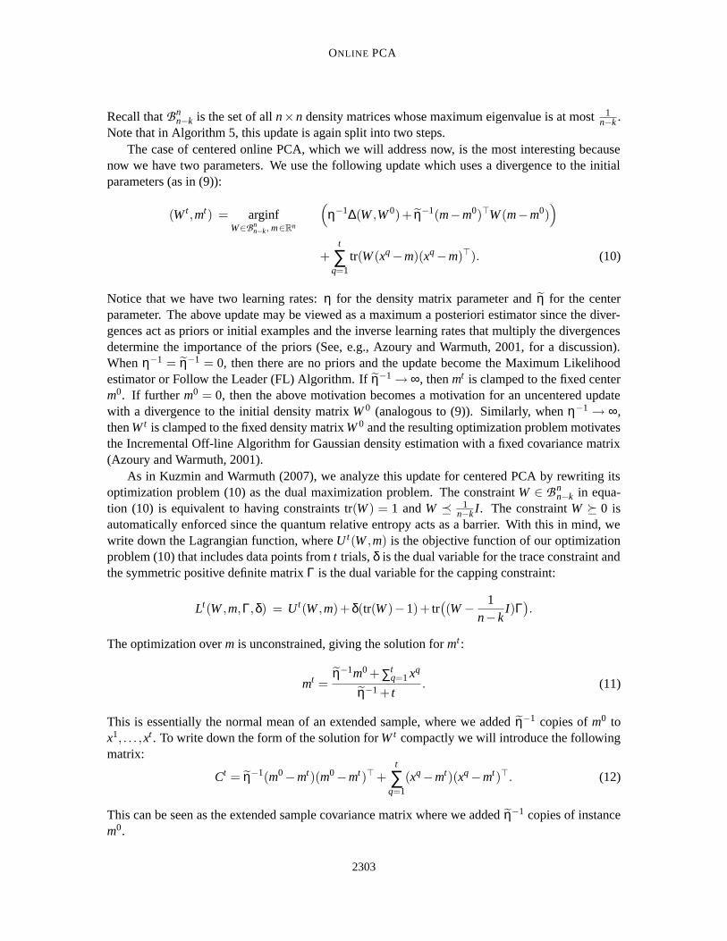
The case of centered online PCA, which we will address now, is the most interesting becausenow we have two parameters. We use the following update which uses a divergence to the initialparameters (as in (9)):
(W t ,mt) = arginfW∈Bn
n−k, m∈Rn
(η−1∆(W ,W 0)+ η−1(m−m0)>W (m−m0)
)
+t
∑q=1
tr(W (xq −m)(xq −m)>). (10)
Notice that we have two learning rates: η for the density matrix parameter and η for the centerparameter. The above update may be viewed as a maximum a posteriori estimator since the diver-gences act as priors or initial examples and the inverse learning rates that multiply the divergencesdetermine the importance of the priors (See, e.g., Azoury and Warmuth, 2001, for a discussion).When η−1 = η−1 = 0, then there are no priors and the update become the Maximum Likelihoodestimator or Follow the Leader (FL) Algorithm. If η−1 → ∞, then mt is clamped to the fixed centerm0. If further m0 = 0, then the above motivation becomes a motivation for an uncentered updatewith a divergence to the initial density matrix W 0 (analogous to (9)). Similarly, when η−1 → ∞,then W t is clamped to the fixed density matrix W 0 and the resulting optimization problem motivatesthe Incremental Off-line Algorithm for Gaussian density estimation with a fixed covariance matrix(Azoury and Warmuth, 2001).
As in Kuzmin and Warmuth (2007), we analyze this update for centered PCA by rewriting itsoptimization problem (10) as the dual maximization problem. The constraint W ∈ B n
n−k in equa-tion (10) is equivalent to having constraints tr(W ) = 1 and W � 1
n−k I. The constraint W � 0 isautomatically enforced since the quantum relative entropy acts as a barrier. With this in mind, wewrite down the Lagrangian function, where U t(W ,m) is the objective function of our optimizationproblem (10) that includes data points from t trials, δ is the dual variable for the trace constraint andthe symmetric positive definite matrix Γ is the dual variable for the capping constraint:
Lt(W ,m,Γ,δ) = U t(W ,m)+δ(tr(W )−1)+ tr((W − 1
n− kI)Γ).
The optimization over m is unconstrained, giving the solution for mt :
mt =η−1m0 +∑t
q=1 xq
η−1 + t. (11)
This is essentially the normal mean of an extended sample, where we added η−1 copies of m0 tox1, . . . ,xt . To write down the form of the solution for W t compactly we will introduce the followingmatrix:
Ct = η−1(m0 −mt)(m0 −mt)> +t
∑q=1
(xq −mt)(xq −mt)>. (12)
This can be seen as the extended sample covariance matrix where we added η−1 copies of instancem0.
2303

WARMUTH AND KUZMIN
Setting the derivatives to zero and solving (see Tsuda et al. 2005 for similar derivation), weobtain the following form of W t in terms of the dual variables δ′ = ηδ and Γ:
W t(δ′,Γ) = exp(logW 0 −ηCt −δ′I −ηΓ).
The constraint tr(W ) = 1 is enforced by choosing δ′ = log tr(exp(logW 1 −ηCt −Γ)). By substitut-ing W t(δ′,Γ) and the formula for mt into the Lagrangian Lt and simplifying, we obtain the followingdual problem:
max�0
Lt(Γ), where Lt(Γ) = −η−1 log tr(exp(logW 0 −ηCt −ηΓ))− tr(Γ)
n− k. (13)
Let Γt be the optimal solution of the dual problem above and let capd(W ) be the density matrixobtained when the capping Algorithm 4 is applied to the vector of eigenvalues of W and cappingparameter d. This lets us express W t as:
W t =exp(logW 0 −ηCt −ηΓt)
tr(exp(logW 0 −ηCt −ηΓt))= capn−k
( exp(logW 0 −ηCt)
tr(exp(logW 0 −ηCt))
). (14)
For the analysis we express mt and Ct as online updates:
Lemma 7 The estimates of mean and covariance can be updated as follows:
mt =(η−1 + t −1)mt−1 + xt
η−1 + t= mt−1 − 1
η−1 + t(mt−1 − xt),
Ct = Ct−1 +η−1 + t −1
η−1 + t(xt −mt−1)(xt −mt−1)>
Proof The update rule for mt is easy to verify. For the update of Ct , we start by expanding theexpression (12) for Ct−1:
Ct−1 = η−1(m0(m0)>−m0(mt−1)>−mt−1(m0)> +mt−1(mt−1)>)
+t−1
∑q=1
(mt−1(mt−1)>− xq(mt−1)>−mt−1(xq)> + xq(xq)>)
=t−1
∑q=1
xq(xq)> +(η−1 + t −1)mt−1(mt−1)>
−(η−1m0 +t−1
∑q=1
xq)(mt−1)>−mt−1(η−1m0 +t−1
∑q=1
xq)> + η−1m0(m0)>.
By substituting
η−1m0 +t−1
∑q=1
xq = (η−1 + t −1)mt−1
we get the following:
Ct−1 =t−1
∑q=1
xq(xq)>− (η−1 + t −1)mt−1(mt−1)> + η−1m0(m0)>.
2304

ONLINE PCA
Algorithm 6 Centered Online PCA Algorithm
input: 1 ≤ k < n and an initial offset m0, initial density matrix W 0 ∈ Bnn−k, C0 = 0
for t = 1 to T doPerform eigendecomposition W t−1 = W ωW >
Decompose ω into a convex combination ∑ j p jr j of at most n corners r j
by applying Algorithm 2 with d = n− kDraw corner r = r j with probability p j
Form a matrix corner R = W diag(r)W >
Form a rank k projection matrix Pt−1 = I − (n− k)RReceive data instance vector xt
Incur compression loss‖(xt −mt−1)−Pt−1(xt −mt−1)‖2
2 = tr((I −Pt−1)(xt −mt−1)(xt −mt−1)>)and expected compression loss (n− k)tr(W t−1(xt −mt−1)(xt −mt−1)>)
Update:
mt = mt−1 − 1η−1 + t
(mt−1 − xt) (15)
Ct = Ct−1 +η−1 + t −1
η−1 + t(xt −mt−1)(xt −mt−1)> (16)
Wt
=exp(logW 0 −ηCt)
tr(exp(logW 0 −ηCt))
W t = capn−k(Wt),
where capn−k(A) applies Algorithm 4 to the vector of eigenvalues of Aend for
Now the update for C can be written as:
Ct = Ct−1 +(η−1 + t −1)mt−1(mt−1)> + xt(xt)>− (η−1 + t)mt(mt)>.
Substituting the left update for mt from the statement of the lemma and simplifying gives the desiredonline update for Ct .
: All the steps for the Centered Online PCA Algorithm are summarized as Algorithm 6. We alreadyreasoned that the capping and decomposition steps are O(n2). The remaining expensive step ismaintaining the eigendecomposition of the covariance matrix for computing the matrix exponential.Using standard rank one update techniques for the eigendecomposition of a symmetric matrix, thiscosts O(n2) per trial (see, e.g., Gu and Eisenstat, 1994).
6.2 Regret Bound for Centered PCA
The following theorem proves a regret bound for our Centered Online PCA Algorithm.
2305

WARMUTH AND KUZMIN
Theorem 8 For any data sequence x1, . . . ,xT , initial center value m0 such that ‖xt −m0‖2 ≤ 12 , any
density matrix U ∈ Bnn−k and any center vector m, the following bound holds:
compalg ≤η compU ,m +∆(U ,W 0)+ηη−1(m−m0)>U(m−m0)
1− exp(−η)+1+ log
(1+
T −1η−1 +1
)
where
compalg =T
∑i=1
tr(W t−1(xt −mt−1)(xt −mt−1)>)
is the overall expected compression loss of the centered online PCA Algorithm 6 and
compU ,m =T
∑i=1
tr(U(xt −m)(xt −m)>)
is the total compression loss of comparison parameters (U ,m).
Proof There are two main proof methods for the expert setting. The first is based on Bregmanprojections and was used so far in this paper. The second uses the value of the optimization problemdefining the update as a potential and then shows that the drop of this value (Kivinen and Warmuth,1999; Cesa-Bianchiand and Lugosi, 2006) is lower bounded by a constant times the per trial lossof the algorithm. Here we use a refinement of the second method that expresses the value of theoptimization problem in terms of its dual. These variations of the second method were developedin the context of boosting (Warmuth et al., 2006; Liao, 2007) and in the conference paper (Kuzminand Warmuth, 2007) where we enhanced the Uncentered Online PCA Algorithm of this paper witha kernel.
For our problem the value6 of optimization problem (10) is vt = U t(W t ,mt) and this equals thevalue of the dual problem Lt(Γt) where Γt maximizes the dual problem (13).
We want to establish the following key inequality:
vt − vt−1 ≥ η−1(1− e−η)(
tr(W t−1(xt −mt−1)(xt −mt−1)>)− 1η−1 + t
). (17)
Since Γt optimizes the dual function Lt and Γt−1 is a non-optimal choice, Lt(Γt) ≥ Lt(Γt−1) andtherefore
vt − vt−1 = Lt(Γt)− Lt−1(Γt−1) ≥ Lt(Γt−1)− Lt−1(Γt−1) (18)
Substituting Lt and Lt−1 from (13) into the right hand side of this inequality gives the following:
Lt(Γt−1)− Lt−1(Γt−1)
= −η−1 log tr(exp(logW 0 −ηCt −ηΓt−1))+η−1 log tr(exp(logW 0 −ηCt−1 −ηΓt−1))
= −η−1 log tr(exp(logW 0 −ηCt −ηΓt−1 − log tr(exp(logW 0 −ηCt−1 −ηΓt−1))).
Now we expand Ct and use the covariance matrix update from Lemma 7:
Lt(Γt−1)− Lt−1(Γt−1) = −η−1 log tr(exp(logW 0 −ηCt−1 −ηΓt−1
− log tr(exp(logW 0 −ηCt−1 −ηΓt−1))−ηη−1 + t −1
η−1 + t(xt −mt−1)(xt −mt−1)>)).
6. Optimization problem (10) minimizes a convex function subject to linear cone constraint. Since this problem has astrictly feasible solution, strong duality is implied by a generalized Slater condition (Boyd and Vandenberghe, 2004).
2306

ONLINE PCA
The first four terms under the matrix exponential form logW t−1, which can be seen from the firstexpression for W t−1 from (14):
Lt(Γt−1)− Lt−1(Γt−1)
= −η−1 log tr(
exp(logW t−1 −ηη−1 + t −1
η−1 + t(xt −mt−1)(xt −mt−1)>)
).
Going back to (18) we get the inequality:
vt − vt−1
≥−η−1 log tr(
exp(logW t−1 −ηη−1 + t −1
η−1 + t(xt −mt−1)(xt −mt−1)>)
).
This expression for the drop of the value is essentially the same expression that is normally boundedin the proof of online variance minimization algorithm in Warmuth and Kuzmin (2006a). Usingthose techniques (assumption in the theorem implies that that ‖xt −mt−1‖2
2 ≤ 1 and all the necessaryinequalities hold) we get the following inequality:
−η−1 log tr(
exp(logW t−1 −ηη−1 + t −1
η−1 + t(xt −mt−1)(xt −mt−1)>)
)
≥ η−1 η−1 + t −1η−1 + t
(1− e−η)tr(W t−1(xt −mt−1)(xt −mt−1)>).
W t−1 is a density matrix and its eigenvalues are at most 1. And by assumption, norm of xt −mt−1 isat most 1. Therefore, the loss tr(W t−1(xt −mt−1)(xt −mt−1)>) is also at most 1. We split the factor
in front of the loss as η−1+t−1η−1+t = 1− 1
η−1+t , upper bounding the loss by 1 for the second part andleaving it as is for the first. With this (17) is obtained.
Note that the trace in the inequality (17) is the loss of the algorithm at trial t. Summation over tand telescoping gives us:
vT − v0 ≥ η−1(1− e−η)(
compalg −T
∑t=1
1η−1 + t
).
We consider the left side first: v0 is equal to zero, and vT is a minimum of optimization problem(10), thus we can make it bigger by substituting arbitrary non-optimal values U and m. Index Tmeans the optimization problem is defined with respect to the entire data sequence, therefore theloss term becomes the loss of the comparator. On the right side we use the following bound on the
sum of generalized harmonic series: ∑Tt=1
1η−1+t ≤ 1+ log
(1+ T−1
η−1+1
). Overall, we get:
η−1∆(U ,W 0)+ η−1(m−m0)>U(m−m0)+ compU ,m
≥ η−1(1− e−η)
(compalg −
(1+ log
(1+
T −1η−1 +1
))).
Moving things over and dividing results in the bound of the theorem.
As discussed before, when η−1 = η−1 = 0, then the algorithm becomes the FL Algorithm. Whenη−1 → ∞, then mt is clamped to m0, that is, the update for the center (11,15) becomes mt = m0 and
2307

WARMUTH AND KUZMIN
is vacuous. Also in that case the term ηη−1(m−m0)>U(m−m0) in the upper bound of Theorem8 is infinity unless the comparison center m is m0 as well. If m0 = 0 in addition to η−1 → ∞, thenwe call this the uncentered version of Algorithm 6: this version simply ignores step (15) and in (16)uses mt−1 = 0. Our original Algorithm 5 for uncentered PCA as well as the uncentered version ofAlgorithm 6 have the same regret bound7 of Theorem 6. Recall however that the two algorithmswere motivated differently: Algorithm 5 trades off divergence to the last parameter with the loss inthe last trial, whereas Algorithm 6 trades off a divergence to the initial parameter matrix with thetotal loss in all past trials. If all constraints are equality constraints, then the two algorithms arethe same. However, capping introduces inequality constraints and therefore the two algorithms aredecidedly not the same. Both algorithm can behave quite differently experimentally (Section 8).The difference between the two algorithms will become important in the followup paper (Kuzminand Warmuth, 2007), where we were only able to use a kernel with the algorithm that trades off adivergence to the initial parameter matrix with the total loss in all past trials.
Similarly, when η−1 → ∞, then W t is clamped to W 0 and the algorithm degenerates to a pre-viously analyzed algorithm, the Incremental Off-line Algorithm for Gaussian density estimationwith fixed covariance matrix (Azoury and Warmuth, 2001). For this restricted density estimationproblem, improved regret bounds were proven for the Forward Algorithm which further shrinks theestimate of the mean towards the initial mean. So far we were not able to improve our regret boundfor uncentered PCA using additional shrinkage towards the initial mean.
The statement of the theorem requires strong initial knowledge about the center of the datasequence we are about to observe: the condition of the theorem says that our data sequence has tobe contained in a ball of radius 1
2 around m0. This can be relaxed by using m0 = 0 and η−1 = 0,which corresponds to using standard empirical mean for mt . Now it suffices to assume that data iscontained in some ball, but we are not required to know where exactly that ball is. The appropriateassumption and the change to the bound are detailed in the following corollary.
Corollary 9 For any data sequence x1, . . . ,xT that can be covered by a ball of radius 12 , that is,
‖xt1 − xt2‖2 ≤ 1 and that also has the bound on the norm of instances ‖xt‖2 ≤ R, any density matrixU ∈Bn
n−k and any center vector m, the total expected loss of centered online PCA Algorithm 6 beingused with parameters η−1 = 0 and m0 = 0 is bounded as follows:
compalg ≤η compU ,m +∆(U ,W 0)
1− e−η + logT +R2,
Proof The ball assumption means that the empirical mean mt−1 and any element of the data se-quence are not too far from each other: ‖mt−1 − xt‖2 ≤ 1. Thus we can still use the Inequality (17),for all trials but the first one, where we haven’t seen any data points yet. Summing the drops of thevalue starting from t = 1 we get:
vT − v1 ≥ η−1(1− e−η)
(T
∑t=2
tr(W t−1(xt −mt−1)(xt −mt−1)>)−T
∑t=2
1t
).
7. The remaining +1 is an artifact of our bound on the harmonic sum.
2308
ONLINE PCA
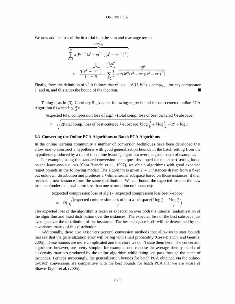
We now add the loss of the first trial into the sum and rearrange terms:compalg︷ ︸︸ ︷
T
∑t=1
tr(W t−1(xt −mt−1)(xt −mt−1)>)
≤ η(vT −≥0︷︸︸︷v1 )
1− e−η +
≤logT︷︸︸︷T
∑t=2
1t
+
≤R2
︷ ︸︸ ︷tr(W 0(x1 −m0)(x1 −m0)>) .
Finally, from the definition of vT it follows that vT ≤ η−1∆(U ,W 0)+ compU ,m, for any comparatorU and m, and this gives the bound of the theorem.
Tuning η as in (3), Corollary 9 gives the following regret bound for our centered online PCAAlgorithm 6 (when k ≤ n
2 ):
(expected total compression loss of alg.) - (total comp. loss of best centered k-subspace)
≤√
2(total comp. loss of best centered k-subspace)k lognk
+ k lognk
+R2 + logT.
6.3 Converting the Online PCA Algorithms to Batch PCA Algorithms
In the online learning community a number of conversion techniques have been developed thatallow one to construct a hypothesis with good generalization bounds in the batch setting from thehypotheses produced by a run of the online learning algorithm over the given batch of examples.
For example, using the standard conversion techniques developed for the expert setting basedon the leave-one-out loss (Cesa-Bianchi et al., 1997), we obtain algorithms with good expectedregret bounds in the following model: The algorithm is given T − 1 instances drawn from a fixedbut unknown distribution and produces a k-dimensional subspace based on those instances; it thenreceives a new instance from the same distribution. We can bound the expected loss on the newinstance (under the usual norm less than one assumption on instances):
(expected compression loss of alg.) - (expected compression loss best k-space)
= O(√ (expected compression loss of best k-subspace)k log n
k
T+
k log nk
T
).
The expected loss of the algorithm is taken as expectation over both the internal randomization ofthe algorithm and fixed distribution over the instances. The expected loss of the best subspace justaverages over the distribution of the instances. The best subspace itself will be determined by thecovariance matrix of this distribution.
Additionally, there also exist very general conversion methods that allow us to state boundsthat say that the generalization error will be big with small probability (Cesa-Bianchi and Gentile,2005). These bounds are more complicated and therefore we don’t state them here. The conversionalgorithms however, are pretty simple: for example, one can use the average density matrix ofall density matrices produced by the online algorithm while doing one pass through the batch ofinstances. Perhaps surprisingly, the generalization bounds for batch PCA obtained via the online-to-batch conversions are competitive with the best bounds for batch PCA that we are aware ofShawe-Taylor et al. (2005).
2309

WARMUTH AND KUZMIN
7. Lower Bounds
We first prove some lower bounds for the simplest online algorithm that just predicts with the modelthat has incurred minimum loss so far (the Follow the Leader (FL) Algorithm). After that we give alower bound for uncentered PCA that shows that the algorithm presented in this paper is optimal ina very strong sense.
Our first lower bound is in the standard expert setting. We assume that there is a deterministictie-breaking rule, because by adding small perturbations, ties can always be avoided in this con-struction. It is easy to see that the following adversary strategy forces FL to have loss n times largerthan the loss of the best expert chosen in hindsight: in each trial have the expert chosen by FL incurone unit of loss. Note that the algorithm incurs loss one in each trial, whereas the loss of the bestexpert is bT
n c after T trials. We conclude that the loss of FL can be by a factor of n larger than theloss of the best expert.
We next show that for the set expert case, FL can be forced to have loss at least nd times the loss
of the best set of size d. In this case FL chooses a set of size d of minimum loss and the adversaryforces the lowest loss expert in the set chosen by FL to incur one unit of loss. The algorithm againincurs loss one in each trial, but the loss of the best set lies in the range d [b T
n c,dTn e]. Thus in this
case the loss of FL can be by a factor of nd larger than the loss of the best set of size d.
When rephrased i.t.o. compression losses, FL picks a set of size n− d whose complementaryset of size d has minimum compression loss. We just showed that the total compression loss of FLcan be at least n
d times the compression loss of the best subset of size n−d.We can lift the above lower bound for sets to the case of uncentered PCA. Now d = n− k and k
is the rank of the subspace we want to compress onto. To simplify the argument, we let the first ninstances be small multiples of the standard basis vectors. More precisely, xt = tε et , for 1 ≤ t ≤ nand small real ε. These instances cause the uncentered data covariance matrix ∑n
t=1 xtx>t to be adiagonal matrix. Also, if ε is small enough then the loss in the first n trials is negligible. From nowon FL always chooses a unique set of d = n− k standard basis vectors of minimum loss and theadversary chooses a standard basis vector with the lowest loss in the set as the next instance. So thelower bound argument essentially reduces to the set case, and FL can be forced to have compressionloss n
n−k times the loss of the compression loss of the best k dimensional subspace.So far we have shown that our online algorithms are better than the simplistic FL Algorithm
since their compression losses are at most one times the loss of the best plus essentially a squareroot term. We now show that the constant in front of the square root term is rather tight as well. Forthe expert setting (d = 1) this was already done:
Theorem 10 (Theorem C.3. of the journal version Helmbold and Warmuth 2008 of the conferencepaper Helmbold and Warmuth 2007.) For all ε > 0 there exists nε such that for any number ofexperts n ≥ nε, there exists a Tε,n where for any number of trials T ≥ Tε,n the following holds forany algorithm in the expert setting: there is a sequence of T trials with n experts for which the lossof the best expert is at most T/2 and the regret of the algorithm is at least (1− ε)
√(T/2) logn.
In the expert model used in this paper, we follow Freund and Schapire (1997) and assume thatthe losses of the experts in each trial are specified by a loss vector in [0,1]N . There is a relatedmodel (studied earlier), where the experts produce predictions in each trial. After receiving thosepredictions the algorithm produces its own prediction and receives a label. The loss of the experts
2310

ONLINE PCA
and algorithm is the absolute value of the difference between the predictions and the label, respec-tively (Littlestone and Warmuth, 1994). The above theorem actually holds for this model of onlinelearning with the absolute loss (when all predictions are in [0,1] and the labels are in {0,1}), andthe model used in this paper may be seen as the special case where the prediction of the algorithm isformed by simply averaging the predictions of the experts (Freund and Schapire, 1997). Thereforeany lower bound for the described expert model with absolute loss immediately holds for the expertmodel where the loss is specified by a loss vector.
Note that the regret bounds for the Hedge Algorithm discussed at the end of Section 3 havean additional factor of 2 in the square root term. By choosing a prediction function other than theweighted average, the factor of 2 can be avoided in the expert model with the absolute loss, andthe upper and lower bounds for the regret have the same constant in front of the square root term(provided that N and T are large enough) (Cesa-Bianchi et al., 1997; Cesa-Bianchiand and Lugosi,2006).
The above lower bound theorem immediately generalizes to the case of set experts. Partitionthe experts into d blocks of size n
d (assume d divides n). For any algorithm and block, constructa sequence of length T as before. During the sequence for one block, the experts for all the otherblocks have loss zero. The loss of the best set of size d on the whole sequence of length T d is atmost T d/2 and the regret, that is, the loss of the algorithm on the sequence minus the loss of thebest set of size d, is lower bounded by
(1− ε)d√
T2
lognd
= (1− ε)√
dT2
d lognd.
Rewritten in terms of compression losses for compression sets of size k (i.e., d = n− k), the lowerbound on the compression loss regret becomes
(1− ε)√
compression loss of best k-subset (n− k) logn
n− k. (19)
Note that the upper bound (4) obtained by our algorithm for learning as well as the best subset isessentially a factor of
√2 larger than this lower bound.
Finally, we lift the above lower bound for subsets to a lower bound for uncentered PCA. In thesetup for uncentered PCA, the instance matrix at trial t is St = xt(xt)>, where xt has 2-norm at most1. For the lower bound we need the instance matrix St to be an arbitrary symmetric matrix witheigenvalues in [0,1]. As discussed before Section 5.1, the upper bound for uncentered PCA stillholds for these more general instance matrices.
To lift the lower bound for subsets to uncentered PCA, we simply replace the loss vector `t bythe instance matrix St = diag(`t). At trial t, the PCA algorithm uses the density matrix W t−1 andincurs expected loss tr(W t−1 diag(`t)) = diag(W t−1) ·`t . Note that the diagonal vector diag(W t−1) isa probability vector. Thus the PCA algorithm doesn’t have any advantage from using non-diagonaldensity matrices and the lower bound reduces to the set case. We conclude that the lower bound(19) also holds for the compression loss regret of uncentered PCA algorithms when the instancematrices are allowed to be symmetric matrices with eigenvalues in [0,1]. Again the correspondingupper bound (7) is essentially a factor of
√2 larger.
2311

WARMUTH AND KUZMIN
Figure 3: The data sequence used for thefirst experiment switches be-tween three different subspaces.It is split into three segments.Within each segment, the datais drawn from a different 20-dimensional Gaussian with arank 2 covariance matrix. Weplot the first three coordinatesof each data point. Differentcolors/symbols denote the datapoints that came from the threedifferent subspaces.
Figure 4: The blue/solid curve is the total loss of uncen-tered online PCA Algorithm 5 for the data se-quence described in Figure 3 (with n = 20,k = 2and η = 1). The algorithm uses internal ran-domization for choosing a subspace and there-fore the curve is actually the average total lossover 50 runs for the same data sequence. Theerror bars (one standard deviation) indicate thevariance of the algorithm. The black/dash-dottedcurve plots the same for the uncentered versionof Algorithm 6 (again η = 1). The visible bumpsin the curves correspond to places in the data se-quence where it shifts from one subspace to an-other. The red/dashed curve is the total loss ofthe best projection matrix determined in hind-sight (i.e., loss of batch uncentered PCA). Thegreen/dotted curve is the total loss of the Followthe Leader Algorithm.
8. Simple Experiments
The regret bounds we prove for our online PCA algorithms hold for arbitrary sequences of instances.In other words, they hold even if the instances are produced by an adversary which aims to makethe algorithm have large regret. In many cases, natural data does not have a strong adversarialnature and even the simple Follow the Leader Algorithm might have small regret against the bestsubspace chosen in hindsight. However, natural data commonly shifts with time. It is on such time-changing data sets that online algorithms have an advantage. In this section we present some simpleexperiments that bring out the ability of our online algorithms to adapt to data that shifts with time.
For our first experiment we constructed a simple synthetic data set of time-changing nature.The data sequence is divided into three equal intervals, of 500 points each. Within each intervaldata points are picked at random from a multivariate Gaussian distribution on R
20 with zero mean.
2312

ONLINE PCA
Figure 5: Behavior of the Uncentered Online PCA Algorithm 5 when data shifts from one subspace toanother. First shift for one of the runs in Figure 4 is shown. We show the projection matrices thathave the highest probability of being picked by the algorithm in a given trial. Since k = 2, eachsuch matrix Pt can be seen as a 2-dimensional ellipse in R
20: the ellipse is formed by points Ptxfor all ‖x‖2 = 1. We plot the first three coordinates of this ellipse. The transition sequence startswith the algorithm focused on the optimal projection matrix for the first subset of data and endswith essentially the optimal matrix for the second subset. The depicted transition takes about 60trials and only every 5th trial is plotted.
The covariance matrices for the Gaussians were picked at random but constrained to rank 2, thusensuring that the generated points lie in some 2-dimensional subspace. The generated points withnorm bigger than one were normalized to 1. The data set is graphically represented in Figure 3,which plots the first three dimensions of each one of the data points. Different colors/symbolsindicate data points that came from the three different subspaces.
In Figure 4 we plot the total compression loss for some of the algorithms introduced in thispaper. For the sake of simplicity we restrict ourselves to uncentered PCA. Here the data dimensionn is 20 and the subspace dimension k is 2. We plot the total loss of the following algorithms as afunction of the trial number: the FL Algorithm, the original uncentered PCA Algorithm 5 and theuncentered version of Algorithm 6. For the latter two algorithms we need to select a learning rate.One possibility is to choose the learning rate that optimizes our upper bound on the regret of thealgorithms (3). Since the bound is the same for both algorithms this choice of η is also the same:the choice depends on an upper bound on the compression loss of the batch algorithm. Pluggingin the actual compression loss of the batch algorithm gives η = 0.12. In practice, heuristics can beused to tune η. For the experiment of Figure 4 we simply chose η = 1. Recall that our online PCAalgorithms decompose their density matrix parameter W t into a convex combination of projectionmatrices using the deterministic Algorithm 2. However, the PCA algorithms then randomly selectone of the k dimensional projection matrices in the convex combination with probability equal toits coefficient. This introduces randomness into the execution of the algorithm even when run on afixed data sequence. We run the algorithms 50 times and plot the average total loss as a function
2313

WARMUTH AND KUZMIN
of t for the fixed data sequence depicted in Figure 3. We also indicate the variance of this totalloss with error bars of one standard deviation. Note again that the average and variance is w.r.t.internal randomization of the algorithm. The bumps in the loss curves of Figure 4 correspond to theplaces in the data sequence where it shifts from one subspace to another. When the loss curve of analgorithm flattens out then the algorithm has learned the correct subspace for the current segment.For example, Figure 5 depicts how the density matrix of the uncentered PCA Algorithm 5 (η = 1)transitions around a segment boundary.
The FL Algorithm (which coincides with the uncentered version of Algorithm 10 when η → ∞)learns the first segment really quickly, but it does not recover during the later segments. The originaluncentered PCA Algorithm 5 (with η = 1) recovers in each segment, whereas the uncentered versionof Algorithm 6 (with η = 1) does not recover as quickly and has higher total loss on this datasequence. Recall that both online algorithms for uncentered PCA have the same regret bound againstthe best fixed offline comparator.
In Figure 4 we also plot the compression loss of the best subspace selected in hindsight by run-ning batch uncentered PCA (dashed/red line). The data set we generated is not well approximatedby a single 2-dimensional subspace, since it consists of three different 2-dimensional subspaces. Asa result, the overall loss of the fixed subspace is higher than the loss of both of our uncentered onlinePCA algorithms that to a varying extent were able to switch between the different 2-dimensionalsubspaces.
There are many heuristics for detecting switches of the data. For example one could simplycheck for a performance loss of any algorithm in a suitably chosen final segment. However, suchalgorithms are often unwieldy and are hard to tune when the data in difference segments are notdrastically different. Note that for the Uncentered Online PCA Algorithm presented in this paperwe only have provable good regret bounds against the best fixed subspace chosen offline (based onthe entire data sequence). (In Figure 4 both of our online algorithms beat the offline comparatorand thus have negative regret against this simple comparator.) Ideally we would like measure regretagainst stronger offline comparators that can exploit the shifting nature of the data. In the expertsetting there is a long line of research where the offline algorithm is allowed to partition the datasequence into s segments and pick the best subspace for each of the s segments. There are simplemodifications of the online algorithm in the experts setting that have good regret bounds against thebest partition of size s (see, e.g., Herbster and Warmuth, 1998). Naturally, the regret bounds growwith the number of segments s. The modifications that are needed to achieve these regret bounds aresimple: insert an additional update step at the end of each trial that mixes a little bit of the uniformdistribution into the weight vector. In the context of uncentered PCA this amounts to adding thefollowing update at the end of each trial:
W t = (1−α)W t +αIn.
We claim that it is easy to again lift the techniques developed in the expert setting to PCA and provethe analogous regret bounds against the best partition.
The following subtle modification of the mixing rule leads to algorithms with even more in-teresting properties. If the algorithm mixes in a little bit of the average of all past weight vectorsinstead of the uniform vector, then it is able to switch quickly to experts that have been good atsome time in the past. This has been called the “long-term memory” property of such algorithms.In the context of uncentered PCA, this amounts the following additional update step for the density
2314

ONLINE PCA
Figure 6: Long term memory effect when mixing in past average is added to the uncentered online PCAAlgorithm 5. The data sequence is comprised of several segments, each one of two hundredrandomly sampled images of the same person but with different facial expressions and lightingconditions. These segments are indicated with dotted lines and are labeled with the face of theperson that was used to generate the segment. The plot depicts the regret of the uncentered onlinePCA Algorithm 5 (η = 1) with added mixing update (20) (α = .001). The regret is w.r.t. theindicated partition of size six.
matrix:
W t = (1−α)W t +α∑t−1
q=0W q
t. (20)
We performed another experiment that demonstrates this “long-term memory” effect by addingupdate (20) to the uncentered online PCA Algorithm 5: For this experiment we used face image datafrom Yale-B data set. A segmented data sequence was constructed by sampling the face images,where each segment contained images of the same person, but with different facial expressions,lighting conditions, etc. Figure 6 plots the regret of our uncentered online PCA Algorithm 5 againstthe best partition of size 6 chosen offline (η = 1,α = .001). In the picture the segment boundaries areindicated with dotted lines and the face below each segment shows the person who’s pictures weresampled during that section. Note that our online algorithm doesn’t have knowledge of segmentboundaries. The first segment shows the typical behavior of online algorithms: the regret growsinitially, but then flattens out once the algorithm converges to the best solution for that segment.Thus the “bump” in the regret curve is due to the fact that the algorithm has to learn a new segmentof pictures from a different person. By comparing the bumps of different segments we see that theyare significantly smaller in segments where the algorithm encounters pictures from a person that it
2315

WARMUTH AND KUZMIN
has previously seen: the algorithm “remembers” subspaces that were good in the past. These smallbumps can be seen in segments 3,5 and 6 in our data set. For additional plots of long-term memoryeffects in the expert setting see Bousquet and Warmuth (2002). Our experiments are preliminary andwe did not formally prove regret bounds for shifting comparators in PCA setting, but such boundsare straightforwardly obtained using the methodology from this paper and Bousquet and Warmuth(2002).
9. Conclusions
We developed a new set of techniques for learning as well as a low dimensional subspace. We firstdeveloped the algorithms in the expert case and then lifted these algorithms and bounds to the matrixcase as essentially done in Tsuda et al. (2005); Warmuth and Kuzmin (2006a). The new insight isto represent our uncertainty over the subspace as a density matrix with capped eigenvalues. Weshow how to decompose such a matrix into a mixture of n subspaces of the desired rank. In the caseof PCA the seemingly quadratic compression loss can be rewritten as a linear loss of our matrixparameter. Therefore a random subspace chosen from the mixture has the same expected loss as theloss of the parameter matrix.
Similar techniques (albeit not capping) have been used recently for learning permutations (Helm-bold and Warmuth, 2008): Instead of maintaining a probability vector over the n! permutations, theparameter used in that paper is a convex combination of permutation matrices which is an n× ndoubly stochastic matrix. This matrix can be efficiently decomposed into a mixture of O(n2) per-mutation matrices. If the loss is linear, then a random permutation chosen from the mixture has thesame expected loss as the loss of the doubly stochastic parameter matrix.
When the loss is convex and not linear (as for example the quadratic loss in the generalizationof linear regression to matrix parameters Tsuda et al. 2005), then our new capping trick can still beapplied to the density matrix parameter. In this case, the online loss of the capped density matrix canbe shown to be close to the loss of the best low dimensional subspace. However the quadratic lossof the capped density matrix (which is a convex combination of subspaces) can be much smallerthan the convex combination of the losses of the subspaces. The bounds of that paper only hold forthe smaller loss of the capped density matrix and not for the expected loss of the subspace sampledfrom the convex combination represented by the capped density matrix.
Our new capping technique is interesting in its own right. Whereas the vanilla multiplicativeupdate on n experts with exponential factors is prone to be unstable because it tends to go into acorner of the simplex (by putting all weight on the currently best expert), the technique of cappingthe weight at 1
d keeps a set of at least d experts alive. In some sense the capping has the same effectas a “super predator” has on a biological system: such a predator specializes on the most frequentspecies of prey, preventing the dominance of any particular species and thus preserving variety. SeeWarmuth (2007a) for a discussion of the relationships of our updates to biological systems.
Following Kivinen and Warmuth (1997); Helmbold et al. (1999), we motivate our updates bytrading off a parameter divergence against a loss divergence. In our case, the parameter divergenceis always a capped relative entropy and the loss divergence is simply linear. It would be interestingto apply the capping trick to the logistic loss used in logistic regression. The logistic loss can beseen as a relative entropy between the desired probabilities of the outcomes and the predicted prob-abilities of the outcomes obtained by applying a sigmoid function to the linear activations (Kivinenand Warmuth, 2001). For “capped logistic regression”, linear constraints would be added to the op-
2316

ONLINE PCA
timization problem defining the updates that cap the predicted probabilities of the outcomes. Thiswould lead to versions of logistic regression where the loss favors a small set of outcomes insteadof a single outcome.
The algorithms of this paper belong to the family of multiplicative updates, that is, the parame-ters are updated by multiplicative factors of exponentials. In the matrix case the updates make useof the matrix log and matrix exponential. There is a second family of updates that does additiveparameter updates. In particular, there are additive online updates for PCA (Crammer, 2006). Thelatter update family has the key advantage that they can be easily used with kernels. However, ina recent conference paper (Kuzmin and Warmuth, 2007) we also were able to give a special casewhere the multiplicative updates could be enhanced with a kernel. In this case the instance ma-trices are outer products xt(xt)> and are replaced by φ(x)t(φ(xt))>. In particular, the online PCAalgorithms of this paper can be “kernelized” this way.
In PCA the instance matrices are symmetric matrices xt(xt)> and we seek a low rank symmetricsubspace that approximates the instances well. In a recent conference paper we showed in a slightlydifferent context how to generalize our methods to the case of “asymmetric” matrices of arbitraryshape. Using those techniques, the online PCA algorithms of this paper can be generalized to theasymmetric case: now the instance matrices are rank one n×m matrices of the form xt(xt)>, wherex and x are vectors of dimension n and m, respectively. In the asymmetric case, the underlyingdecomposition is the SVD decomposition instead of the eigendecomposition.
There are two technical open problems that arise in this paper. We gave a number of dynamicprogramming algorithms, such as the one given for the set expert problem. If the loss range for theindividual experts is [0,1] then the loss range for the set experts is [0,d] when d is the size of theset. The straightforward application of results for the Hedge Algorithm leads to extra factors of din the regret bounds for set experts. We avoided these factors using our capping trick. However,the question is whether the same bounds (without the d factors) hold for the dynamic programmingalgorithm as well. There is a different fundamental algorithmic technique for dealing with structuraldomains: the Follow the Perturbed Leader Algorithm (Kalai and Vempala, 2005). The second openproblem is how to adapt this algorithm to online PCA and prove bounds for it that don’t contain theextra d factors.
Finally, independent of what theoretical progress might have been achieved in this paper, we stillhave to find a convincing experimental setting where our new online PCA algorithms are indispens-able. The update time of our algorithms is O(n2) and further time improvements via approximationsor lazy evaluation might be needed to make the algorithms widely applicable.
Acknowledgments
Thanks to Allen Van Gelder for valuable discussions re. Algorithm 2.
References
K. Azoury and M. K. Warmuth. Relative loss bounds for on-line density estimation with the expo-nential family of distributions. Journal of Machine Learning, 43(3):211–246, June 2001. Specialissue on Theoretical Advances in On-line Learning, Game Theory and Boosting, edited by YoramSinger.
2317

WARMUTH AND KUZMIN
R. Bhatia. Matrix Analysis. Springer, Berlin, 1997.
O. Bousquet and M. K. Warmuth. Tracking a small set of experts by mixing past posteriors. Journalof Machine Learning Research, 3:363–396, 2002.
S. Boyd and L. Vandenberghe. Convex Optimization. Cambridge University Press, 2004.
L. M. Bregman. The relaxation method of finding the common point of convex sets and its applica-tion to the solution of problems in convex programming. USSR Computational Mathematics andPhysics, 7:200–217, 1967.
Y. Censor and A. Lent. An iterative row-action method for interval convex programming. Journalof Optimization Theory and Applications, 34(3):321–353, July 1981.
N. Cesa-Bianchi and C. Gentile. Improved risk tail bounds for on-line algorithms. In NIPS, 2005.
N. Cesa-Bianchi, Y. Freund, D. Haussler, D. P. Helmbold, R. E. Schapire, and M. K. Warmuth. Howto use expert advice. Journal of the ACM, 44(3):427–485, May 1997.
N. Cesa-Bianchiand and G. Lugosi. Prediction, Learning, and Games. Cambridge University Press,2006.
K. Crammer. Online tracking of linear subspaces. In Proceedings of the 19th Annual Conferenceon Learning Theory (COLT 06), Pittsburg, June 2006. Springer.
Y. Freund and R. E. Schapire. A decision-theoretic generalization of on-line learning and an appli-cation to Boosting. Journal of Computer and System Sciences, 55(1):119–139, August 1997.
M. Gu and S. Eisenstat. A stable and efficient algorithm for the rank-one modification of thesymmetric eigenproblem. SIAM Journal on Matrix Analysis and Applications, 15(4):1266–1276,October 1994.
D. Helmbold and M. K. Warmuth. Learning permutations with exponential weights. In Proceedingsof the 20th Annual Conference on Learning Theory (COLT07). Springer, 2007.
D. Helmbold and M. K. Warmuth. Learning permutations with exponential weights. Submittedjournal version, August 2008.
D. P. Helmbold, J. Kivinen, and M. K. Warmuth. Relative loss bounds for single neurons. IEEETransactions on Neural Networks, 10(6):1291–1304, November 1999.
M. Herbster and M. K. Warmuth. Tracking the best expert. Machine Learning, 32(2):151–178,1998. Earlier version in 12th ICML, 1995.
M. Herbster and M. K. Warmuth. Tracking the best linear predictor. Journal of Machine LearningResearch, 1:281–309, 2001.
A. Kalai. Simulating weighted majority with FPL. Private communication, 2005.
A. Kalai and S. Vempala. Efficient algorithms for online decision problems. J. Comput. Syst. Sci.,71(3):291–307, 2005. Special issue Learning Theory 2003.
2318

ONLINE PCA
J. Kivinen and M. K. Warmuth. Averaging expert predictions. In Computational Learning Theory,4th European Conference, EuroCOLT ’99, Nordkirchen, Germany, March 29-31, 1999, Proceed-ings, volume 1572 of Lecture Notes in Artificial Intelligence, pages 153–167. Springer, 1999.
J. Kivinen and M. K. Warmuth. Additive versus exponentiated gradient updates for linear prediction.Information and Computation, 132(1):1–64, January 1997.
J. Kivinen and M. K. Warmuth. Relative loss bounds for multidimensional regression problems.Machine Learning, 45(3):301–329, 2001.
J. Kivinen, M. K. Warmuth, and B. Hassibi. The p-norm generalization of the LMS algorithmfor adaptive filtering. Journal of IEEE Transactions on Signal Processing (to appear), 54(5):1782–1793, May 2005.
D. Kuzmin and M. K. Warmuth. Optimum follow the leader algorithm. In Proceedings of the 18thAnnual Conference on Learning Theory (COLT 05), pages 684–686. Springer, June 2005. Openproblem.
D. Kuzmin and M. K. Warmuth. Online Kernel PCA with entropic matrix updates. In ICML ’07:Proceedings of the 24th International Conference on Machine Learning. ACM Press, June 2007.
J. Liao. Totally Corrective Boosting Algorithms that Maximize the Margin. PhD thesis, Universityof California at Santa Cruz, June 2007.
N. Littlestone and M. K. Warmuth. The weighted majority algorithm. Inform. Comput., 108(2):212–261, 1994. Preliminary version in in FOCS 89.
A. W. Marshall and I. Olkin. Inequalities: Theory of Majorization and its Applications. AcademicPress, 1979.
R. Rockafellar. Convex Analysis. Princeton University Press, 1970.
T. D. Sanger. Optimal unsupervised learning in a single-layer linear feedforward neural network.Neural Networks, 2:459–473, 1989.
J. Shawe-Taylor, C. K. I. Williams, N. Cristianini, and J. S. Kandola. On the eigenspectrum ofthe gram matrix and the generalization error of kernel-PCA. IEEE Transactions on InformationTheory, 51(7):2510–2522, 2005. URL http://dx.doi.org/10.1109/TIT.2005.850052.
E. Takimoto and M. K. Warmuth. Path kernels and multiplicative updates. Journal of MachineLearning Research, 4:773–818, 2003.
K. Tsuda, G. Ratsch, and M. K. Warmuth. Matrix exponentiated gradient updates for on-line learn-ing and Bregman projections. Journal of Machine Learning Research, 6:995–1018, June 2005.
M. K. Warmuth. The blessing and the curse of the multiplicative updates. Work in progress,unpublished manuscript., 2007a.
M. K. Warmuth. When is there a free matrix lunch. In Proc. of the 20th Annual Conference onLearning Theory (COLT 07). Springer, June 2007b. Open problem.
2319

WARMUTH AND KUZMIN
M. K. Warmuth and D. Kuzmin. Online variance minimization. In Proceedings of the 19th AnnualConference on Learning Theory (COLT 06), Pittsburg, June 2006a. Springer.
M. K. Warmuth and D. Kuzmin. Randomized PCA algorithms with regret bounds that are logarith-mic in the dimension. In Advances in Neural Information Processing Systems 19 (NIPS 06). MITPress, December 2006b.
M. K. Warmuth, J. Liao, and G. Ratsch. Totally corrective boosting algorithms that maximize themargin. In ICML ’06: Proceedings of the 23rd International Conference on Machine Learning,pages 1001–1008, New York, NY, USA, 2006. ACM Press.
2320