randomized prediction games for adversarial machine learning · randomized prediction games for...
TRANSCRIPT
1
Randomized Prediction Games forAdversarial Machine Learning
Samuel Rota Bulo, Member, IEEE, Battista Biggio, Member, IEEE, Ignazio Pillai, Member, IEEE,Marcello Pelillo, Fellow, IEEE Fabio Roli, Fellow, IEEE
Abstract—In spam and malware detection, attackers exploitrandomization to obfuscate malicious data and increase theirchances of evading detection at test time; e.g., malware codeis typically obfuscated using random strings or byte sequencesto hide known exploits. Interestingly, randomization has alsobeen proposed to improve security of learning algorithms againstevasion attacks, as it results in hiding information about the clas-sifier to the attacker. Recent work has proposed game-theoreticalformulations to learn secure classifiers, by simulating differentevasion attacks and modifying the classification function accord-ingly. However, both the classification function and the simulateddata manipulations have been modeled in a deterministic manner,without accounting for any form of randomization. In this work,we overcome this limitation by proposing a randomized predic-tion game, namely, a non-cooperative game-theoretic formulationin which the classifier and the attacker make randomized strategyselections according to some probability distribution definedover the respective strategy set. We show that our approachallows one to improve the trade-off between attack detectionand false alarms with respect to state-of-the-art secure classifiers,even against attacks that are different from those hypothesizedduring design, on application examples including handwrittendigit recognition, spam and malware detection.
Index Terms—Pattern classification, adversarial learning, gametheory, randomization, computer security, evasion attacks.
I. INTRODUCTION
Machine-learning algorithms have been increasinglyadopted in adversarial settings like spam, malware andintrusion detection. However, such algorithms are notdesigned to operate against intelligent and adaptive attackers,thus making them inherently vulnerable to carefully-craftedattacks. Evaluating security of machine learning against suchattacks and devising suitable countermeasures, are two amongthe main open issues under investigation in the field ofadversarial machine learning [1]–[11]. In this work we focuson the issue of designing secure classification algorithmsagainst evasion attacks, i.e., attacks in which malicioussamples are manipulated at test time to evade detection. Thisis a typical setting, e.g., in spam filtering, where spammersmanipulate the content of spam emails to get them past theanti-spam filters [1], [2], [12]–[14], or in malware detection,where hackers obfuscate malicious software (malware, forshort) to evade detection of either known or zero-day exploits[8], [9], [15], [16]. Although out of the scope of this work,it is worth mentioning here another pertinent attack scenario,referred to as classifier poisoning. Under this setting, the
S. Rota Bulo is with ICT-Tev, Fondazione Bruno Kessler, Trento, ItalyM. Pelillo is with DAIS, Universita Ca’ Foscari, Venezia, ItalyB. Biggio, I. Pillai, F. Roli are with DIEE, University of Cagliari, Italy
attacker can manipulate the training data to mislead classifierlearning and cause a denial of service; e.g., by increasing thenumber of misclassified samples [6], [7], [17]–[20].
To date, several authors have addressed the problem ofdesigning secure learning algorithms to mitigate the impact ofevasion attacks [1], [6], [10], [11], [21]–[27] (see Sect. VII forfurther details). The underlying rationale of such approachesis to learn a classification function that accounts for potentialmalicious data manipulations at test time. To this end, theinteractions between the classifier and the attacker are modeledas a game in which the attacker manipulates data to evadedetection, while the classification function is modified to clas-sify them correctly. This essentially amounts to incorporatingknowledge of the attack strategy into the learning algorithm.However, both the classification function and the simulateddata manipulations have been modeled in a deterministicmanner, without accounting for any form of randomization.
Randomization is often used by attackers to increase theirchances of evading detection, e.g., malware code is typicallyobfuscated using random strings or byte sequences to hideknown exploits, and spam often contains bogus text randomlytaken from English dictionaries to reduce the “spamminess”of the overall message. Surprisingly, randomization has alsobeen proposed to improve classifier security against evasionattacks [3], [6], [28]. In particular, it has been shown thatrandomizing the learning algorithm may effectively hide in-formation about the classification function to the attacker,requiring her to select a less effective attack (manipulation)strategy. In practice, the fact that the adversary may notknow the classification function exactly (i.e., in a deterministicsense) decreases her (expected) payoff on each attack sample.This means that, to achieve the same expected evasion rateattained in the deterministic case, the attacker has to increasethe number of modifications made to the attack samples [28].
Motivated by the aforementioned facts, in this work wegeneralize static prediction games, i.e., the game-theoreticalformulation proposed by Bruckner et al. [10], [11], to accountfor randomized classifiers and data manipulation strategies.For this reason, we refer to our game as a randomized predic-tion game. A randomize prediction game is a non-cooperativegame between a randomized learner and a randomized attacker(also called data generator), where the player’s strategiesare replaced with probability distributions defined over therespective strategy sets. Our goal is twofold. We do not onlyaim to assess whether randomization helps achieving a bettertrade-off in terms of false alarms and attack detection (withrespect to state-of-the-art secure classifiers), but also whether
arX
iv:1
609.
0080
4v1
[cs
.LG
] 3
Sep
201
6
2
our approach remains more secure against attacks that aredifferent from those hypothesized during design. In fact, giventhat our game considers randomized players, it is reasonableto expect that it may be more robust to potential deviationsfrom its original hypotheses about the players’ strategies.
The paper is structured as follows. Randomized predictiongames are presented in Sect. II, where sufficient conditions forthe existence and uniqueness of a Nash equilibrium in thesegames are also given. In Sect. III we focus on a specific gameinstance involving a linear Support Vector Machine (SVM)learner, for which we provide an effective method to findan equilibrium by overcoming some computational problems.We discuss how to enable the use of nonlinear (kernelized)SVMs in Sect. IV. In Sect. V we report a simple example tointuitively explain how the proposed methods enforce securityin adversarial settings. Related work is discussed in Sect. VII.In Sect. VI we empirically validate the soundness of theproposed approach on an handwritten digit recognition task,and on realistic adversarial application examples involvingspam filtering and malware detection in PDF files. Notably,to evaluate robustness of our approach and state-of-the-artsecure classification algorithms, we also consider attacks thatdeviate from the models hypothesized during classifier design.Finally, in Sect. VIII, we summarize our contributions andsketch potential directions for future work.
II. RANDOMIZED PREDICTION GAMES
Consider an adversarial learning setting involving two ac-tors: a data generator and a learner.1 The data generatorproduces at training time a set D = xi, yini=1 ⊆ X ×Y of ntraining samples, sampled from an unknown probability distri-bution. Sets X and Y denote respectively the input and outputspaces of the learning task. At test time, the data generatormodifies the samples in D to form a new dataset D ⊆ X ×Y ,reflecting a test distribution, which differs in general fromthe training distribution and it is not available at trainingtime. We assume binary learners, i.e. Y = −1,+1, andwe assume also that the data transformation process leaves thelabels of the samples in D unchanged, i.e., D = (xi, yi)ni=1.Hence, a perturbed dataset will simply be represented in termsof a tuple X = (x1, . . . ,xn) ∈ X n, each element beingthe perturbation of the original input sample xi, while weimplicitly assume the label to remain yi. The role of the learneris to classify samples x ∈ X according to the predictionfunction h(x) = sign[f(x;w)], which is expressed in termsof a linear generalized decision function f(x;w) = w>φ(x),where w ∈ Rm, x ∈ X and φ : X → Rm is a feature map.
Static prediction games have been introduced in [11] bymodeling the learner and the data generator as players ofa non-cooperative game that we identify as l-player and d-player, respectively. The strategies of l-player correspond tothe parametrizationsw of the prediction function f . The strate-gies of the data generator, instead, are assumed to live directlyin the feature space, by regarding X = (x>1 , . . . , x
>n )> ∈ Rmn
as a data generator strategy, where xi = φ(xi). By doingso, the decision function f becomes linear in either players’
1We adopt here the same terminology used in [11].
strategies. Each player is characterized also by a cost functionthat depends on the strategies played by either players. Thecost function of d-player and l-player are denoted by cd andcl, respectively, and are given by
cl(w, X) = ρlΩl(w) +
n∑
i=1
`l(w>xi, yi) , (1)
cd(w, X) = ρdΩd(X) +n∑
i=1
`d(w>xi, yi) , (2)
where w ∈ Rm is the strategy of l-player, X ∈ Rmn is thestrategy of the d-player, and yi denotes the label of xi as perD. Moreover, ρd/l > 0 is a trade-off parameter, `d/l(w>xi, y)measures the loss incurred by the l/d-player when the decisionfunction yields w>xi for the ith training sample while thetrue label is y, and Ωd/l can be regarded as a penalizationfor playing a specific strategy. For the d-player, this termquantifies the cost of perturbing D in feature space.
The goal of our work is to introduce a randomizationcomponent in the model of [11], particularly to what concernsthe players’ behavior. To this end, we take one abstractionstep with respect to the aforementioned prediction game,where we let the learner and the data generator sample theirplaying strategy in the prediction game from a parametrizeddistribution, under the assumption that they are expected cost-minimizing (a.k.a. expected utility-maximizing). By doing so,we introduce a new non-cooperative game that we call ran-domized prediction game between the l-player and the d-playerwith strategies being mapped to the possible parametrizationsof the players’ respective distributions, and cost functionsbeing expected costs under the same distributions.
A. Definition of randomized prediction game
Consider a prediction game as described before. We in-ject randomness in the game by assigning each player aparametrized probability distribution, i.e., pl(w;θl) for thelearner and pd(X;θd) for the data generator, that governs theplayers’ strategy selection. Players are allowed to select theparametrization θl and θd for the respective distributions. Forany choice of θl, the l-player plays a strategy w sampled frompl(·;θl). Similarly, for any choice of θd, the d-player plays astrategy X sampled from pd(·;θd). If the players adhere to thenew rules, we obtain a randomized prediction game.
A randomized prediction game is a non-cooperative gamebetween a learner (l-player) and data generator (d-player) thathas the following components:
1) an underlying prediction game with cost functionscl/d(w, X) as defined in (1) and (2),
2) two parametrized probability distributions pl/d(·;θl/d)with parameters in Θl/d,
3) Θl/d are non-empty, compact and convex subsets of afinite-dimensional metric space Rsl/d .
The sets of parameters Θl/d are the pure strategy sets (a.k.a.action spaces) for the l-player and d-player, respectively. Thecosts functions of the two players, which quantify the costthat each player incurs when a strategy profile (θl,θd) ∈Θl ×Θd is played, coincide with the expected costs, denoted
3
by cl/d(θl,θd), that the two players have in the underlyingprediction game if strategies are sampled from pl(·;θl) andpd(·;θd), according to the expected cost-minimizing hypoth-esis:
cl(θl,θd) = Ew∼pl(·;θl)X∼pd(·;θd)
[cl(w, X)] , (3)
cd(θl,θd) = Ew∼pl(·;θl)X∼pd(·;θd)
[cd(w, X)] , (4)
where E[·] denotes the expectation operator. We assume cl/dto be well-defined functions, i.e. the expectations to be finitefor any (θl,θd) ∈ Θl ×Θd. To avoid confusion between cl/dand cl/d, in the remainder of this paper we will refer themrespectively as cost functions, and expected cost functions.
By adhering to a non-cooperative setting, the two playersinvolved in the prediction game are not allowed to communi-cate and they play their strategies simultaneously. Each playerhas complete information of the game setting by knowing theexpected cost function and strategy set of either players. Underrationality assumption, each player’s interest is to achieve thegreatest personal advantage, i.e., to incur the lowest possiblecost. Accordingly, the players are prone to play a Nashequilibrium, which in the context of our randomized predictiongame is a strategy profile (θ?l ,θ
?d) ∈ Θl × Θd such that no
player is interested in changing his/her own playing strategy.In formal terms, this yields:
θ?l ∈ arg minθl∈Θl
cl(θl,θ?d) , θ?d ∈ arg min
θd∈Θd
cd(θ?l ,θd) . (5)
B. Existence of a Nash equilibrium
The existence of a Nash equilibrium of a randomized pre-diction game is not granted in general. A sufficient conditionfor the existence of a Nash equilibrium is thus given below.
Theorem 1 (Existence). A randomized prediction game admitsat least one Nash equilibrium if
(i) cl/d are continuous in Θl ×Θd,(ii) cl(·,θd) is quasi-convex in Θl for any θd ∈ Θd,
(iii) cd(θl, ·) is quasi-convex in Θd for any θl ∈ Θl.
Proof: The result follows directly from the Debreu-Glicksberg-Fan Theorem [29].C. Uniqueness of a Nash equilibrium
In addition to the existence of a Nash equilibrium, it is ofinterest to investigate if the equilibrium is unique. However,determining tight conditions that guarantee the uniqueness ofthe Nash equilibrium for any randomized prediction game ischallenging; in particular, due to the additional dependence ona probability distribution for the learner and the data generator.
We will make use of a classical result due to Rosen [30] toformulate sufficient conditions for the uniqueness of the Nashequilibrium of randomized prediction games in terms of theso-called pseudo-gradient of the game, defined as
gr =
[rl∇θl
clrd∇θd
cd
], (6)
with any fixed vector r = [rl, rd]> ≥ 0. Specifically, a
randomized prediction game admits a unique Nash equilibriumif the following assumption is verified
Assumption 1.(i) cl/d are twice differentiable in Θl ×Θd,
(ii) cl(·,θd) is convex in Θl for any θd ∈ Θd,(iii) cd(θl, ·) is convex in Θd for any θl ∈ Θl,
and gr is strictly monotone for some fixed r > 0, i.e.,
[gr(θl,θd)− gr(θ′l,θ′d)]>[θl − θ′lθd − θ′d
]> 0 ,
for any distinct strategy profiles (θl,θd), (θ′l,θ′d) ∈ Θl×Θd.2
In his paper, Rosen provides also a useful sufficient condi-tion that guarantees a strictly monotone pseudo-gradient. Thisrequires the Jacobian of the pseudo-gradient, a.k.a. pseudo-Jacobian, given by
Jr =
[rl∇2
θlθlcl rl∇2
θlθdcl
rd∇2θdθl
cd rd∇2θdθd
cd
], (7)
to be positive definite.
Theorem 2. A randomized prediction game admits a uniqueNash equilibrium if Assumption 1 holds, and the pseudo-Jacobian Jr(θl,θd) is positive definite for all (θl,θd) ∈Θl ×Θd and some fixed r > 0.
Proof: Under Assumption 1, the positive definiteness ofJr for all strategy profiles and some fixed vector r > 0implies the strict monotonicity of gr, which in turn impliesthe uniqueness of the Nash equilibrium [30, Thm. 6].
In the rest of the section, we provide sufficient conditionsthat ensure the positive definiteness of the pseudo-Jacobianand thus the uniqueness of the Nash equilibrium via Thm. 2.To this end we decompose cl/d(θl,θd) as follows
cl(θl,θd) = ρlΩl(θl) + Ll(θl,θd) ,
cd(θl,θd) = ρdΩd(θd) + Ld(θl,θd) ,(8)
where Ωl/d and Ll/d are the expected regularization and lossterms given by
Ωl(θl) = Ew∼pl(·,θl)[Ωl(w)] ,
Ωd(θd) = EX∼pd(·,θd)[Ωd(X)] ,
Ll(θl,θd) = Ew∼pl(·;θl)X∼pd(·;θd)
[n∑
i=1
`l(w>xi, yi)
],
Ld(θl,θd) = Ew∼pl(·;θl)X∼pd(·;θd)
[n∑
i=1
`d(w>xi, yi)
].
Moreover, we require the following convexity and differentia-bility conditions on Ωl/s and Ll/d:
Assumption 2.(i) Ωl/d is strongly convex and twice continuously differen-
tiable in Θl/d,(ii) Ll(·,θd) is convex and twice continuously differentiable
in Θl for all θd ∈ Θd, and(iii) Ld(θl, ·) is convex and twice continuously differentiable
in Θd for all θl ∈ Θl.
2Assumption 1.(i) could be relaxed to continuously differentiable.
4
Finally, we introduce some quantities that are used in thesubsequent lemma, which gives sufficient conditions for thepositive-definiteness of the pseudo-Jacobian:
λΩl = inf
θl∈Θl
λmin[∇2θlθl
Ωl(θl)],
λΩd = inf
θd∈Θd
λmin[∇2θdθd
Ωd(θd)],
λLl = inf(θl,θd)∈Θl×Θd
λmin[∇2θlθl
Ll(θl,θd)],
λLd = inf(θl,θd)∈Θl×Θd
λmin[∇2θdθd
Ld(θl,θd)],
τ = sup(θl,θd)∈Θl×Θd
λmax[R(θl,θd)R(θl,θd)
>] ,
where R(θl,θd) = 12
[∇2θlθd
Ll(θl,θd)> +∇2
θdθlLd(θl,θd)
]
and λmax/min give the maximum/minimum eigenvalue of thematrix in input. Note that the quantities listed above are finiteand positive if Assumption 2 holds, given the compactness ofΘl/d.
Lemma 1. If Assumption 2 holds and
(ρlλΩl + λLl )(ρdλ
Ωd + λLd ) > τ
then the pseudo-Jacobian Jr(θl,θd) is positive definite for all(θl,θd) ∈ Θl ×Θd by taking r = (1, 1)>.
Proof: The pseudo-Jacobian in (7) can be written asfollows given the decomposition of cl/d in (8):
Jr =
[ρl∇2
θlθlΩl +∇2
θlθlLl ∇2
θlθdLl
∇2θdθl
Ld ρd∇2θdθd
Ωd +∇2θdθd
Ld
],
where we omitted the arguments of Ωl/d and Ll/d for nota-tional convenience. Let us denote by Jllr , Jldr , Jdlr , and Jddr thefour matrices composing Jr (in top-down, left-right order).
Consider the following matrix:
H =
[Hll Hld
Hdl Hdd
]=
[ρlλ
Ωl + λLl R(θl,θd)
>
R(θl,θd) ρdλΩd + λLd
].
Then we have for all t = (t>l , t>d ) 6= 0
t>Jrt = tJr + J>r
2t>
= tlJllr tl︸ ︷︷ ︸
≥tlHlltl
+ tdJddr td︸ ︷︷ ︸
≥t>d Hddtd
+t>lJldr + Jdl>r
2︸ ︷︷ ︸Hld+Hdl>
td ≥ t>Ht ,
where the under-braced relations follow from the definitions ofλΩl/d, λLl/d and R. Accordingly, the positive-definiteness of Jr
can be derived from the positive-definiteness of matrix H. Toprove the latter, we will show that all roots of the characteristicpolynomial det(H−λI) of H are positive. By properties of thedeterminant3 we have
det(H− λI) = det((ρlλΩl + λLl − λ)I)
· det
((ρdλ
Ωd + λLd − λ)I− S
ρlλΩl + λLl − λ
),
3det
[aI B>
B dI
]= det(aI) det(dI − 1
aBB>) and if USU> is the eigen-
decomposition of BB> then the latter determinant becomes det(U(dI −1aS)U>) = det(dI− 1
aS)
Algorithm 1 Extragradient descent (adapted from [11])Input: Cost functions cl/d; parameter spaces Θl,Θd; a small
positive constant ε.Output: The optimal parameters θl,θd.
1: Randomly select θ(0) = (θ(0)l ,θ
(0)d ) ∈ Θl ×Θd.
2: Set iteration count k = 0, and select σ, β ∈ (0, 1).3: Set r = (rl, rd)
>= (1, ρl/ρd)
>.
4: repeat5: Set d(k) = ΠΘl×Θd
(θ(k) − gr
(θ
(k)l ,θ
(k)d
))− θ(k).
6: Find maximum step size t(k) ∈ βp|p ∈ N s.t.
−gr(θ
(k)l , θ
(k)d
)>
d(k) ≥ σ(∥∥∥d(k)
∥∥∥2
2
),
where θ(k)= θ(k) + t(k)d(k).
7: Set η(k) = − t(k)∥∥∥gr
(θ(k)l ,θ
(k)d
)∥∥∥2
2
gr
(θ
(k)l , θ
(k)d
)>
d(k).
8: Set θ(k+1) = ΠΘl×Θd
(θ(k) − η(k)gr
(θ
(k)l , θ
(k)d
)).
9: Set k = k + 1.10: until
∥∥∥θ(k) − θ(k−1)∥∥∥
2
2≤ ε
11: return θl = θ(k)l , θd = θ
(k)d
where S is a diagonal matrix with the eigenvalues ofR(θl,θd)R(θl,θd)
>. The roots of the first determinant termare all equal to ρlλΩ
l + λLl , which is positive because ρl > 0by construction and λΩ
l > 0 follows from the strong-convexityof Ωl in Assumption 2-i. As for the second determinant term,take the ith diagonal element Sii of S. Then two roots are thesolution of the following quadratic equation
λ2 − λ(a+ b) + ab− Sii = 0 ,
which are given by
λ(i)1,2 = a+ b±
√(a− b)2 + 4Sii .
where a = ρlλΩl + λLl and b = ρdλ
Ωd + λLd . Among the two,
λ(i)2 (the one with the minus) is the smallest one, which is
strictly positive if
ab = (ρlλΩl + λLl )(ρdλ
Ωd + λLd ) > Sii .
Since the condition has to hold for any choice of theeigenvalue Sii in the right-hand-side of the inequality, wetake the maximum one maxi Sii, which coincides withλmax(R(θl,θd)R(θl,θd)
>). We further maximize the latterquantity with respect to (θl,θd) ∈ Θl × Θd, because wewant the result to hold for any parametrization. Therefrom werecover the variable τ and the condition (ρlλ
Ωl +λLl )(ρdλ
Ωd +
λLd ) > τ , which guarantees that all roots of the character-istic polynomial of H are strictly positive for any choice of(θl,θd) ∈ Θl × Θd and, hence, Jr is positive definite overΘl ×Θd.
In addition to Lem. 1, we provide in the supplementarymaterial alternative (stronger) sufficient conditions, which gen-eralize the ones given in [11].
5
D. Finding a Nash equilibrium
From the computational perspective, we can find a Nashequilibrium in our game by exploiting algorithms similar to theones adopted for static prediction games [11]. In particular, weconsider a modified extragradient descent algorithm [11], [31],[32] that finds a solution to the following variational inequalityproblem, provided that gr is continuous and monotone:
gr(θ?l ,θ?d)
>(θ − θ?) ≥ 0 ,∀(θl,θd) ∈ Θl ×Θd , (9)
where θ = [θ>l ,θ>d ]> and similarly for θ?. Any solution θ? to
this problem can be shown to correspond bijectively to a Nashequilibrium of a game having gr as pseudo-gradient [11], [32].
If Theorem 1 holds, the pseudo-Jacobian Jr can be shownto be positive semidefinite, and gr is thus continuous andmonotone. Hence, the variational inequality can be solvedby the modified extragradient descent algorithm given asAlgorithm 1, which is guaranteed to converge to a Nashequilibrium point [31], [33]. The algorithm generates a se-quence of feasible points whose distance from the equilibriumsolution is monotonically decreased. It exploits a projectionoperator ΠΘl×Θd
(θ) to map the input vector θ onto the closestadmissible point in Θl×Θd, and a simple line-search algorithmto find the maximum step t on the descent direction d.4
In the next section, we apply our randomized predictiongame to the case of linear SVM learners, and compute thecorresponding pseudo-gradient, as required by Algorithm 1.
III. RANDOMIZED PREDICTION GAMES FOR SUPPORTVECTOR MACHINES
In this section, we consider a randomized prediction gameinvolving a linear SVM learner [34], and Gaussian distribu-tions as the underlying probabilities pl/d.
The learner. The decision function of the learner is ofthe type f(x;w) = w>φ(x) where the feature map isgiven by φ(x) =
[x> 1
]>. For convenience, we consider
a decomposition of w into[w> b
]>, where w ∈ Rm−1
and b ∈ R. Hence, the decision function can also be writtenas f(x;w) = w>x + b. Accordingly, the input space X isa (m− 1)-dimensional vector space, i.e. X ⊆ Rm−1. Thedistribution pl for the learner is assumed to be Gaussian.In order to guarantee the theoretical existence of the Nashequilibrium through Thm. 1, we assume the parameters ofthe Gaussian distribution to be bounded. For the sake ofclarity, we use in this section axis-aligned Gaussians (i.e. withdiagonal covariance matrices) for our analysis, even thoughgeneral covariances could be adopted as well. Under theseassumptions, we define the strategy set for the learner asΘl =
(µw,σw) ∈ Rm × Rm
+
∩ Bl, where Bl ⊂ Rm × Rm
+
is an application-dependent non-empty, convex, bounded set,restricting the set of feasible parameters. The parameter vec-tors µw and σw encode the mean and standard deviation ofthe axis-aligned Gaussian distributions. The loss function `lof the learner corresponds to the hinge loss of the SVM, i.e.,`l(z, y) = [1−zy]+ with [z]+ = max(0, z), while the strategy
4We refer the reader to [11], [31], [32] (and references therein) for detailedproofs that derive conditions for which d is effectively a descent direction.
penalization term Ωl(w) is the squared Euclidean norm of w.As a result, the cost function cl corresponds to the C-SVMobjective function, and it is convex in w:
cl(w, X) =ρl2‖w‖2 +
n∑
i=1
[1− yi(w>xi + b)]+ . (10)
The data generator. For convenience, we consider X ratherthan X as the quantity undergoing the randomization. Thiscomes without loss of generality, because there is a one-to-one correspondence between xi and xi if we considerthe linear feature map xi = φ(xi) = [x>i , 1]>. Moreover,we assume that samples xi can be perturbed independently.Accordingly, the distribution pd for the data generator fac-torizes as pd(X;θd) =
∏ni=1 pd
(xi;θ
(i)d
), where θd =
(θ(1)d , . . . ,θ
(n)d ). We consider pd
(xi;θ
(i)d
)to be a k-variate
axis-aligned Gaussian distribution with bounded mean andstandard deviation given by θ(i)
d = (µxi,σxi). In summary,
the strategy set adopted for the data generator is given by Θd =∏ni=1 Θ
(i)d , where Θ
(i)d =
(µxi
,σxi) ∈ Rk × Rk
+
∩ Bd.
Here, Bd ⊂ Rk × Rk+ is a non-empty, convex, bounded set.
The loss function `d of the data generator is the hinge lossunder wrong labelling, i.e., `d(z, y) = [1 + zy]+. In thisway the data generator is penalized if the learner correctlyclassifies a sample point. Finally, the strategy penalizationfunction Ωd is the squared Euclidean distance of the perturbedsamples in X from the ones in the original training set D, i.e.Ωd(X) =
∑ni=1 ‖xi − xi‖2. The resulting cost function cd is
convex in X:
cd(w, X) =ρd2
n∑
i=1
‖xi − xi‖2
+n∑
i=1
[1 + yi(w>xi + b)]+ . (11)
Existence of a Nash equilibrium. The proposed random-ized prediction game for the SVM learner admits at least oneNash equilibrium. This can be proven by means of Thm. 1.Indeed, the required continuity of cl/d hold and, as for thequasi-convexity conditions, we can rewrite (3) as follows byexploiting the fact that pl is a Gaussian distribution with meanµw and standard deviation σw:
cl(θl,θd) = Ez∼N (0,I)X∼pd(·;θd)
[cl(µw +D(σw)z, X)] , (12)
where N (0, I) is a m-dimensional standard normal distri-bution and D(σw) is a diagonal matrix having σw on thediagonal. Since cl is convex in its first argument and convexityis preserved under addition of convex functions, positiverescaling, and composition with linear functions, we have thatcl is convex (and thus quasi-convex) in θl = (µw,σw). Asfor the quasi-convexity condition of the data generator’s cost,we can exploit the separability of cd to rewrite (4) as follows:
cd(θl,θd) =n∑
i=1
Ew∼pl(·;θl)z∼N (0,I)
[c(i)d (w,µxi
+D(σxi)z)] ,
where
c(i)d (w,x) =
ρd2‖x− xi‖2 + [1 + yi(w
>xi + b)]+ .
6
Since c(i)d is convex in its second argument, by following
the same reasoning used to show the quasi-convexity of thelearner’s expected cost, we have that each expectation in cd isconvex in θ(i)
d = (µxi,σxi
), 1 ≤ i ≤ n. As a consequence,cd is convex and, hence, quasi-convex in θd, being the sumof convex functions.
Uniqueness of a Nash equilibrium. In the previous sectionwe have shown that cl(·,θd) and cd(θl, ·) are convex asrequired by Assumption 1-(ii-iii). In particular we have thatthe single expected regularization terms Ωl/d(·) and loss termsLl(·,θd), Ld(θl, ·) are convex as well. Moreover, they aretwice-continuously differentiable by having Gaussian distri-butions for pl/d. It is then sufficient to have Ωl/d are stronglyconvex to prove the uniqueness of the Nash equilibrium viaLem. 1. While it is easy to see that Ωd is strongly convex,we have that Ωl is not strongly convex with respect to bdue to the presence of an unregularized bias term b in thelearner. The problem derives from the fact that the SVM itselfmay not have a unique solution when the bias term is presentand non-regularized (see [35], [36] for a characterization ofthe degenerate cases). As a result, the proposed game is notguaranteed to have a unique Nash equilibrium in its actualform. On the other hand, a unique Nash equilibrium maybe obtained by either considering an unbiased SVM, i.e., bysetting b = 0 as in [11], or a regularized bias term, e.g., byadding ε
2b2 to the learner’s objective function with ε > 0. In
both cases, all conditions that ensure the uniqueness of theNash equilibrium via Thm. 2 and Lem. 1 would be satisfied,under proper choices of ρl/d.
It is worth noting however that the necessary and sufficientconditions under which a biased (non-regularized) SVM hasno unique solution are quite restricted [35], [36]. For this rea-son, we believe that uniqueness of the Nash equilibrium couldbe proven also for the biased SVM under mild assumptions.However, this requires considerable effort in trying to relaxthe sufficiency conditions of Rosen [30], which is beyond thescope of our work. We thus leave this challenge to futureinvestigations. Moreover, we believe that enforcing a uniqueNash equilibrium in our game by making the original SVMformulation strictly convex may lead to worse results, similarlyto exploiting convex approximations to solve originally non-convex problems in machine learning [37], [38]. For the abovereasons, in this paper, we choose to retain the original SVMformulation for the learner, by sacrificing the uniqueness ofthe Nash Equilibrium. We nevertheless provide in Sect. V adiscussion of why having a unique Nash Equilibrium is not soimportant in practice for our game, and we empirically showin Sect. VI that our approach can anyway achieve competitiveperformances with respect to other state-of-the-art approaches.
The rest of this section is devoted to showing how to com-pute the pseudo-gradient (6) by providing explicit formulaefor ∇θl
cl and ∇θdcd.
A. Gradient of the learner’s cost
In this section, we focus on computing the gradient∇θl
cl(θl,θd), where cl is defined as in (10). By propertiesof expectation and since w follows an axis-aligned Gaussiandistribution with mean µw and standard deviation σw, we can
reduce the cost of the learner to:
cl(θl,θd) =ρl2
(‖µw‖2 + ‖σw‖2
)
+n∑
i=1
E w∼pl(·;θl)
xi∼pd(·;θ(i)d )
[[1− yi(w>xi + b)]+
], (13)
where we are assuming the following decompositions forthe mean µw =
[µ>w µb
]>and standard deviation σw =[
σ>w σb]>
. The hard part for the minimization is the term inthe expectation, which can not be expressed to our knowledgein a closed-form function of the Gaussian’s parameters. Wethus resort to a Central-Limit-Theorem-like approximation,by regarding si = 1 − yi(w
>xi + b) as a Gaussian-distributed variable with mean µsi and standard deviation σsi ,i.e. si ∼ N (µsi , σsi). In general, si does not follow a Gaussiandistribution, since the product of two normal deviates is notnormally distributed. However, if the number of features kis large, the approximation becomes reasonable. Under thisassumption, we can rewrite the expectation as follows:
E w∼pl(·;θl)
xi∼pd(·;θ(i)d )
[[1− yi(w>xi + b)]+
]
= Esi∼N (µsi,σsi
)[[si]+] . (14)
The mean and variance of the Gaussian distribution in theright-hand-side of Eq. (14) are respectively given by
µsi = E w∼pl(·;θl)
xi∼pd(·;θ(i)d )
[1− yi(w>xi + b)
]
= 1− yi(µ>wµxi+ µb) , (15)
σ2si = V w∼pl(·;θl)
xi∼pd(·;θ(i)d )
[1− yi(w>xi + b)
]
= σ2w>
(σ2xi
+ µ2xi
) + µ2w>σ2xi
+ σ2b , (16)
where V is the variance operator, and we assume that squaringa vector corresponds to squaring each single component.
The expectation in Eq. (14) can be transformed after sim-ple manipulations into the following function involving theGauss error function (integral function of the standard normaldistribution) denoted as erf():
h(µsi , σsi) =σsi√2π
exp
(− µ2
si
2σ2si
)
+µsi2
[1− erf
(− µsi√
2σsi
)]. (17)
The learner’s cost in Eq. (13) can thus be approximated as:
cl(θl,θd) ≈ Ll(µw,σw) =ρl2
(‖µw‖2 + ‖σw‖2
)
+
n∑
i=1
h(µsi(θl), σsi(θl)) . (18)
We can now approximate the gradient ∇θlcl in terms of
∇θlLl. In the following, we denote the Hadamard (a.k.a.
entry-wise) product between any two vectors a and b as ab,
7
and we assume any scalar-by-vector derivative to be a columnvector. The gradients of interest are given as:
∂Ll∂µw
= ρl
[µw0
]+
n∑
i=1
(∂h
∂µsi
∂µsi∂µw
+∂h
∂σ2si
∂σ2si
∂µw
), (19)
∂Ll∂σw
= ρl
[σw0
]+
n∑
i=1
(∂h
∂µsi
∂µsi∂σw
+∂h
∂σ2si
∂σ2si
∂σw
), (20)
where it is not difficult to show that∂h
∂µsi=
1
2
[1− erf
(− 1√
2
µsiσsi
)], (21)
∂h
∂σ2si
=1
2
1√2πσsi
exp
(−1
2
µ2si
σ2si
), (22)
and that∂µsi∂µw
= −yi[µxi
1
],
∂µsi∂σw
= 0 , (23)
∂σ2si
∂µw=
[2σ2
xi µw
0
],
∂σ2si
∂σw= 2σw
[σ2xi
+ µ2xi
1
].
(24)
B. Gradient of the data generator’s costIn this section we turn to the data generator and we focus on
approximating ∇θdcd, where cd is defined as in Eq. (11). We
can separate cd into the sum of n functions acting on each datasample independently, i.e. cd(θl,θd) =
∑ni=1 c
(i)d (θl,θ
(i)d ),
where for each i ∈ 1, . . . , n:
c(i)d (θl,θ
(i)d ) = E w∼pl(·;θl)
xi∼pd(·;θ(i)d )
[ρd2‖xi − xi‖2
+[1 + yi(w>xi + b)]+
]. (25)
By exploiting properties of the expectation and sincepd(·;θ(i)
d ) is an axis-aligned Gaussian distribution with meanµxi
and standard deviation σxi, we can simplify Eq. (25) as:
c(i)d (θl,θ
(i)d ) =
ρd2
(‖µxi
− xi‖2 + ‖σxi‖2)
+ E w∼pl(·;θl)
xi∼pd(·;θ(i)d )
[[1 + yi(w
>xi + b)]+
]. (26)
As in the case of the learner, the expectation is a troublesometerm having the same form of (14), except for an inverted sign.We adopt the same approximation used in Sect. III-A to obtaina closed-form function. Accordingly, ti = 1 + yi(w
>xi +b) is assumed to be normally distributed with mean µti andσti . Then the expectation in Eq. (26) can be approximated ash(µti , σti), where function h is defined as in Eq. (17). Thevariance σ2
ti is equal to σ2si (Eq. 16), while µti is given by:
µti = E w∼pl(·;θl)
xi∼pd(·;θ(i)d )
[1 + yi(w
>xi + b)]
= 1 + yi(µ>wµxi
+ µb) .
The sample-wise cost of the data generator (Eq. 26) canthus be approximated as
c(i)d (θl,θ
(i)d ) ≈ Ld(µxi
,σxi) =
ρd2
(‖µxi
− xi‖2 + ‖σxi‖2)
+ h(µti(θ(i)d ), σti(θ
(i)d )) . (27)
The corresponding gradient is given by
∂Ld∂µxi
= (µxi− xi) + ρd
(∂h
∂µti
∂µti∂µxi
+∂h
∂σ2ti
∂σ2ti
∂µxi
),
(28)
∂Ld∂σxi
= σxi + ρd
(∂h
∂µti
∂µti∂σxi
+∂h
∂σ2ti
∂σ2ti
∂σxi
), (29)
where ∂h∂µti
and ∂h∂σ2
ti
are given as in Eqs. (21)-(22), and
∂µti∂µxi
= yiµw ,∂µti∂σxi
= 0 , (30)
∂σ2ti
∂µxi
= 2σ2w µxi
,∂σ2
ti
∂σxi
= 2σxi(σ2w + µ2
w
). (31)
IV. KERNELIZATION
Our game, as in Bruckner et al. [11], assumes explicitknowledge of the feature space φ, where the data generatoris assumed to randomize the samples x = φ(x). However,in many applications, the feature mapping is only implicitlygiven in terms of a positive semidefinite kernel functionk : X ×X → R that measures the similarity between samplesas a scalar product in the corresponding kernel Hilbert space,i.e., there exists φ : X → R such that k(x,x′) = φ(x)>φ(x′).Note that in this setting the input space X is not restricted to avector space like in the previous section (e.g. it might containgraphs or other structured entities).
For the representer theorem to hold [39], we assume thatthe randomized weight vectors of the learner live in thesame subspace of the reproducing kernel Hilbert space, i.e.,w =
∑j αjφ(xj), where α ∈ Rn. Analogously, we restrict
the randomized samples obtained by the data generator tolive in the span of the mapped training instances, i.e., xi =∑nj=1 ξijφ(xj), where ξi = (ξi1, . . . , ξin)
> ∈ Rn.Now, instead of randomizing w and X, we let the data
generator and the learner randomize Ξ = (ξ1, . . . , ξn) and α,respectively. Moreover, we assume that the expected costs cl/dcan be rewritten in terms of α and Ξ in a way that involves onlyinner products of φ(x), to take advantage of the kernel trick.This is clearly possible for the termw>xi = α>Kξi in (1) and(2), where K is the kernel matrix. Hence, the applicability ofthe kernel trick only depends on the choice of the regularizers.It is easy to see that due to the linearity of the variableshift, existence and uniqueness of a Nash equilibrium in ourkernelized game hold under the same conditions given for thelinear case.5
Although the data generator is virtually randomizing strate-gies in some subspace of the reproducing kernel Hilbertspace, in reality manipulations should occur in the originalinput space. Hence, to construct the real attack samplesxini=1 corresponding to the data generator’s strategy at theNash equilibrium, one should solve the so-called pre-imageproblem, inverting the implicit feature mapping φ−1(Kξi) foreach sample. This problem is in general neither convex, nor
5Note that, on the contrary, manipulating samples directly in the inputspace would not even guarantee the existence of a Nash equilibrium, asthe data generator’s expected cost becomes non-quasi-convex in x for many(nonlinear) kernels, invalidating Theorem 1.

8
−1 −0.5 0 0.5 1−1
−0.5
0
0.5
1
−1 −0.5 0 0.5 1−1
−0.5
0
0.5
1
−1 −0.5 0 0.5 1−1
−0.5
0
0.5
1
−1 −0.5 0 0.5 1−1
−0.5
0
0.5
1
−1 −0.5 0 0.5 1−1
−0.5
0
0.5
1
−1 −0.5 0 0.5 1−1
−0.5
0
0.5
1
−1 −0.5 0 0.5 1−1
−0.5
0
0.5
1
−1 −0.5 0 0.5 1−1
−0.5
0
0.5
1
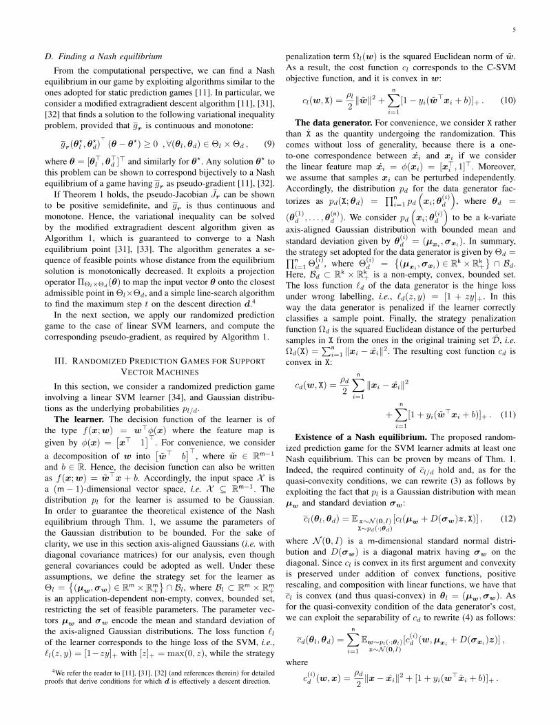
Fig. 1. Two-dimensional examples of randomized prediction games, for SVMs with linear (top) and RBF kernels (bottom). Each row shows how the algorithmgradually converges to a Nash equilibrium. Blue (gray) points represent the legitimate (malicious) class. The mean of each manipulated attack sample is shownas a red point (for clarity, its variance is not shown). The black solid line represents the expected decision boundary, and the green shaded area highlightsits variability within one standard deviation. Note how the linear SVM’s decision boundary tends to shift towards the legitimate class, while the nonlinearboundary provides a better enclosing of the same class. This intuitively allows for a higher robustness to different kinds of attack, as it requires the adversaryto make a higher number of modifications to the attack samples to evade detection, at the expense of a higher number of misclassified legitimate samples.
it admits a unique solution. However, reliable solutions canbe easily found using well-principled approximations [11],[39]. It is finally worth remarking that solving the pre-imageproblem is not even required from the learner’s perspective,i.e., to train the corresponding, secure classification function.
V. DISCUSSION
In this section, we report a simple case study on a two-dimensional dataset to visually demonstrate the effect ofrandomized prediction games on SVM-based learners. From apragmatic perspective, this example suggests also that unique-ness of the Nash Equilibrium should not be taken as a strictrequirement in our game.
An instance of the proposed randomized prediction gamefor a linear SVM and for a non-linear SVM with the RBFkernel is reported in Fig. 1. As one may note from the plots,the main effect of simulating the presence of an attacker thatmanipulates malicious data to evade detection is to causethe linear decision boundary to gradually shift towards thelegitimate class, and the nonlinear boundary to find a betterenclosing of the legitimate samples. This should generallyimprove the learner’s robustness to any kind of evasion at-tempt, as it requires the attacker to mimic more carefully thefeature values of legitimate samples – a task typically harderin several adversarial settings than just obfuscating the contentof a malicious sample to make it sufficiently different from theknown malicious ones [7], [9].
Based on this observation, any attempt aiming to satisfy thesufficient conditions for uniqueness of the Nash Equilibriumwill result in an increase of the regularization strength in eitherthe learner’s or the attacker’s cost function. Indeed, to satisfythe condition in Lem. 1, one could sufficiently increase ρl, ρd,or both. This amounts to increasing the regularization strengthof either players, which in turn reduces in some sense theirpower. Hence, it should be clear that enforcing satisfaction
of the sufficient conditions that guarantee the uniqueness ofthe Nash equilibrium might be counterproductive, by inducingthe learner to weakly enclose the legitimate class, either dueto a too strong regularization of the learners’ parameters, or bylimiting the ability of the attacker to manipulate the malicioussamples, thus allowing the leaner to keep a loose boundary.This will in general compromise the quality of the adversariallearning procedure. This argument shares similarities with theidea of addressing non-convex machine learning problemsdirectly, without resorting to convex approximations [37], [38].
Besides improving classifier robustness, finding a betterenclosure of the legitimate class may however cause a highernumber of legitimate samples to be misclassified as malicious.There is indeed a trade-off between the desired level ofrobustness and the fraction of misclassified legitimate sam-ples. The benefit of using randomization here is to makethe attacker’s strategy less pessimistic than in the case ofstatic prediction games [10], [11], which should allow usto eventually find a better trade-off between robustness andlegitimate misclassifications. This aspect is investigated moresystematically in the experiments reported in the next section.
VI. EXPERIMENTS
In this section we present a set of experiments on hand-written digit recognition, spam filtering, and PDF malwaredetection. Despite handwritten digit recognition is not a properadversarial learning task as spam and malware detection, weconsider it in our experiments to provide a visual interpretationof how secure learning algorithms are capable of improvingrobustness to evasion attacks.
We consider only linear classifiers, as they are a typicalchoice in these settings, and especially in spam filtering [2],[7], [14]. This also allows us to carry out a fair comparisonwith state-of-the-art secure learning algorithms, as they yieldlinear classification functions. We compare our secure linear
9
0 0.5 1 1.5 2 2.50
0.2
0.4
0.6
0.8
1
MNIST 1 vs 3T
P @
FP
=1%
dmax
0 1 2 3 4 50
0.2
0.4
0.6
0.8
1
MNIST 6 vs 7
TP
@F
P=
1%
dmax
0 20 40 600
0.2
0.4
0.6
0.8
1
TREC−07
TP
@F
P=
1%
dmax
0 10 20 30 400
0.2
0.4
0.6
0.8
1
TP
@F
P=
1%
dmax
SVM InvarSVM NashSVM RNashSVM
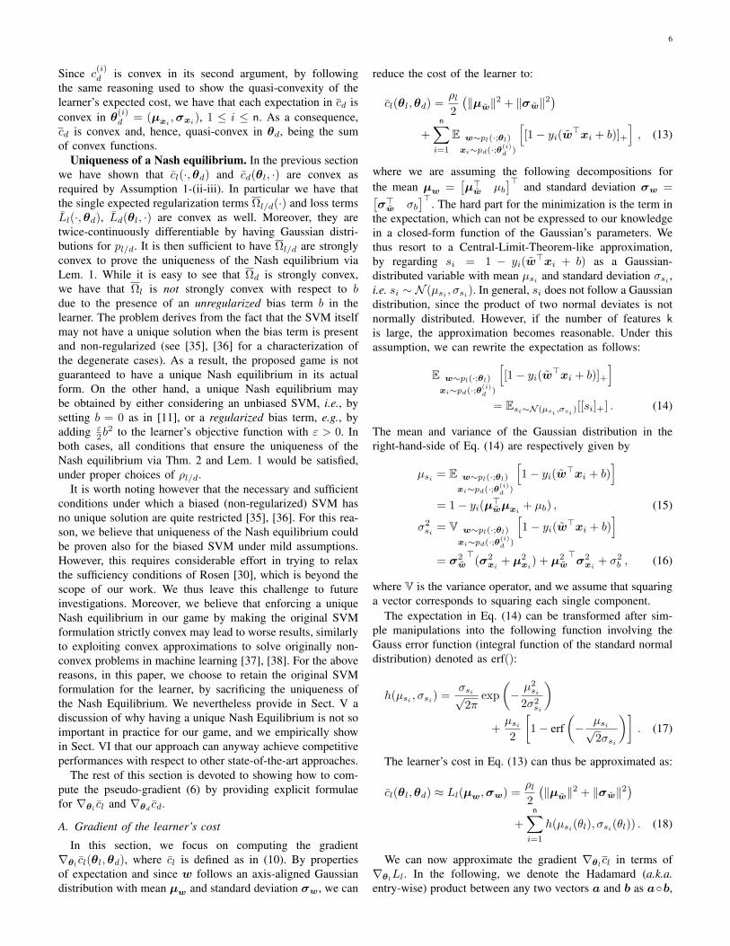
Fig. 2. Security evaluation curves, reporting the average TP at FP=1% (along with its standard deviation, shown with error bars) against an increasing amountof manipulations to the attack samples (measured by dmax), for handwritten digit (first and second plot), spam (third plot), and PDF (fourth plot) data.
SVM learner (Sect. III) with the standard linear SVM imple-mentation [40], and with the state-of-the-art robust classifiersInvarSVM [21], [22], and NashSVM [11] (see Sect. VII).
The goal of these experiments is to test whether these securealgorithms work well also under attack scenarios that differfrom those hypothesized during design – a typical settingin security-related tasks; e.g., what happens if game-basedclassification techniques like that proposed in this paper andNashSVM are used against attackers that exploit a differentattack strategy, i.e., attackers that may not act rationallyaccording to the hypothesized objective function? What hap-pens when the attacker does not play at the expected Nashequilibrium? These are rather important questions to address,as we do not have any guarantee that real-world attackers willplay according to the hypothesized objective function.
Security evaluation. To address the above issues, weconsider the security evaluation procedure proposed in [7].It evaluates the performance of the considered classifiersunder attack scenarios of increasing strength. We consider theTrue Positive (TP) rate (i.e., the fraction of detected attacks)evaluated at 1% False Positive (FP) rate (i.e., the fractionof misclassified legitimate samples) as performance measure.We evaluate the performance of each classifier in the absenceof attack, as in standard performance evaluation techniques,and then start manipulating the malicious test samples tosimulate attacks of different strength. We assume a worst-caseadversary, i.e., an adversary that has perfect knowledge of theattacked classifier, since we are interested in understanding theworst-case performance degradation. Note however that otherchoices are possible, depending on specific assumptions onthe adversary’s knowledge and capability [7], [13], [14]. Inthis setting, we assume that the optimal (worst-case) samplemanipulation x∗ operated by the attacker is obtained bysolving the following optimization problem:
x∗ ∈ arg minx
yf(x;w),
s.t. d(x, xi) ≤ dmax,(32)
where y is the malicious class label, d(x,xi) measures thedistance between the perturbed sample x and the ith maliciousdata sample xi (in this case, we use the `2 norm, as done by theconsidered classifiers). The maximum amount of modificationsis bounded by dmax, which is a parameter representing theattack strength. It is obvious that the more modificationsthe adversary is allowed to make on the attack samples, the
higher the performance degradation incurred by the classifieris expected to be. Accordingly, the performance of more secureclassifiers is expected to degrade more gracefully as the attackstrength increases [7], [14].
The solution of the above problem is trivial when weconsider linear classifiers, the Euclidean distance, and x isunconstrained: it amounts to setting x∗ = xi − ydmax
w||w|| . If
x lies within some constrained domain, e.g. [0, 1], then onemay consider a simple gradient descent with box constraintson x (see, e.g., [9]). If x takes on binary values, e.g., 0, 1,then the attack amounts to switching from 0 to 1 or vice-versathe value of a maximum of dmax features which have beenassigned the highest absolute weight values by the classifier.In particular, if y wk > 0 (y wk < 0) and the k-th featuresatisfies xik = 1 (xik = 0), then x∗k = 1 (x∗k = 0) [7], [14].
Parameter selection. The considered methods require set-ting different parameters. From the learners’ perspective, wehave to tune the regularization parameter C for the standardlinear SVM and InvarSVM, while we respectively have ρ−1
and ρl for NashSVM and for our method. In addition, therobust classifiers require setting the parameters of their at-tacker’s objective. For InvarSVM, we have to set K, i.e., thenumber of modifiable features, while for NashSVM and forour method, we have to set the value of the regularizationparameter ρ+1 and ρd, respectively. Further, to guaranteeexistence of a Nash Equilibrium point, we have to enforcesome box constraints on the distribution’s parameters. For theattacker, we restrict the mean of the attack points to lie in [0, 1](as the considered datasets are normalized in that interval), andtheir variance in [10−3, 0.5]. For the learner, the variance ofw is allowed to vary in [10−6, 10−3], while its mean takesvalues on [−W,W ], where W is optimized together with theother parameters. All the above mentioned parameters are setby performing a grid-search on the parameter space (C, ρ−1,ρd ∈ 0.01, 0.1, 1, 10, 100; K ∈ 8, 13, 25, 30, 47, 52, 63;ρ+1, ρd ∈ 0.01, 0.05, 0.1, 1, 10; W ∈ 0.01, 0.05, 0.1, 1),and retaining the parameter values that maximize the areaunder the security evaluation curve on a validation set. Thereason is to find a parameter configuration for each method thatattains the best average robustness over all attack intensities(values of dmax), i.e. the best average TP rate at FP=1%.A. Handwritten Digit Recognition
Similarly to [21], we focus on two two-class sub-problemsof discriminating between two distinct digits from the MNIST
10
Original InvarSVMSVM NashSVM RNashSVM
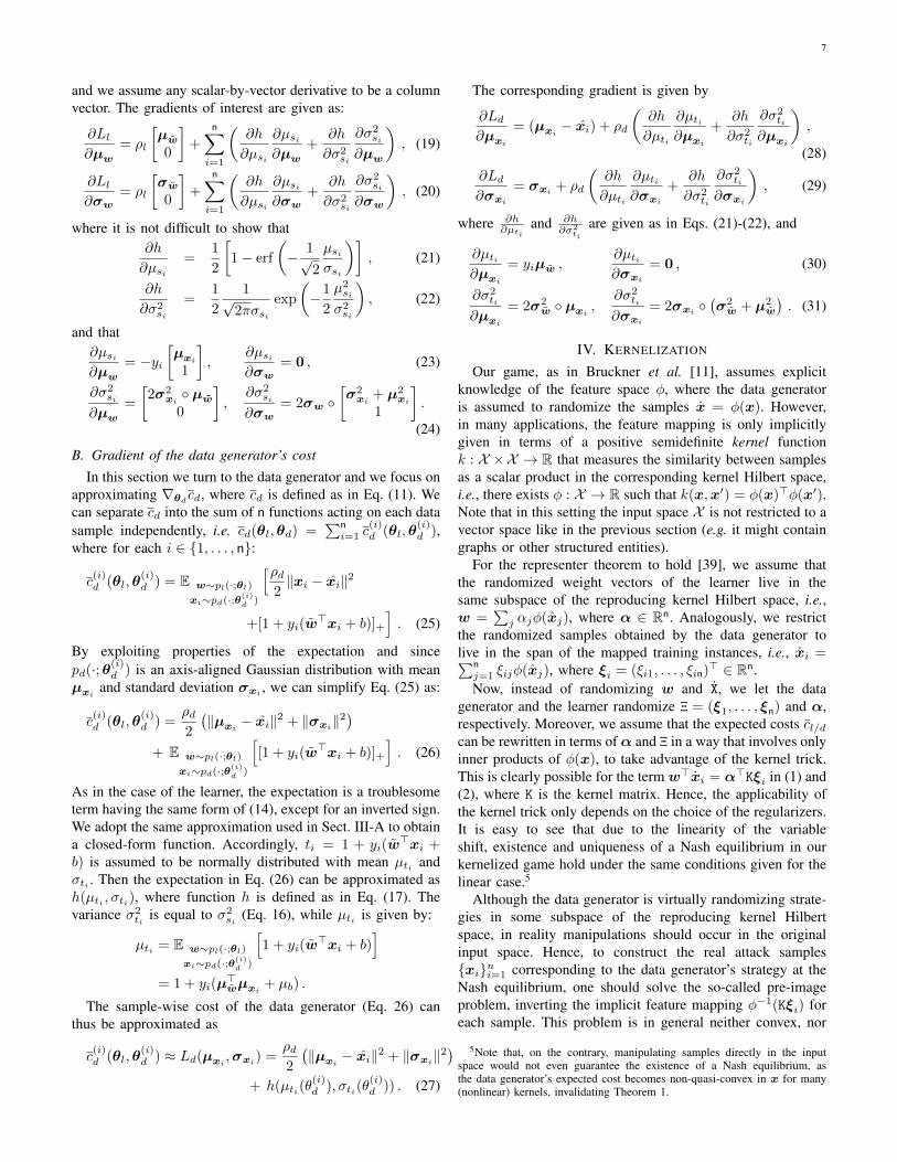
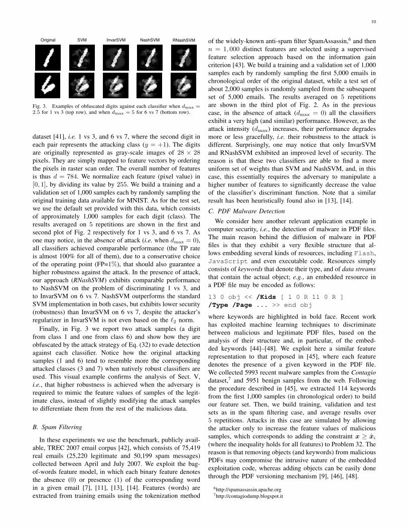
Fig. 3. Examples of obfuscated digits against each classifier when dmax =2.5 for 1 vs 3 (top row), and when dmax = 5 for 6 vs 7 (bottom row).
dataset [41], i.e. 1 vs 3, and 6 vs 7, where the second digit ineach pair represents the attacking class (y = +1). The digitsare originally represented as gray-scale images of 28 × 28pixels. They are simply mapped to feature vectors by orderingthe pixels in raster scan order. The overall number of featuresis thus d = 784. We normalize each feature (pixel value) in[0, 1], by dividing its value by 255. We build a training and avalidation set of 1,000 samples each by randomly sampling theoriginal training data available for MNIST. As for the test set,we use the default set provided with this data, which consistsof approximately 1,000 samples for each digit (class). Theresults averaged on 5 repetitions are shown in the first andsecond plot of Fig. 2 respectively for 1 vs 3, and 6 vs 7. Asone may notice, in the absence of attack (i.e. when dmax = 0),all classifiers achieved comparable performance (the TP rateis almost 100% for all of them), due to a conservative choiceof the operating point (FP=1%), that should also guarantee ahigher robustness against the attack. In the presence of attack,our approach (RNashSVM) exhibits comparable performanceto NashSVM on the problem of discriminating 1 vs 3, andto InvarSVM on 6 vs 7. NashSVM outperforms the standardSVM implementation in both cases, but exhibits lower security(robustness) than InvarSVM on 6 vs 7, despite the attacker’sregularizer in InvarSVM is not even based on the `2 norm.
Finally, in Fig. 3 we report two attack samples (a digitfrom class 1 and one from class 6) and show how they areobfuscated by the attack strategy of Eq. (32) to evade detectionagainst each classifier. Notice how the original attackingsamples (1 and 6) tend to resemble more the correspondingattacked classes (3 and 7) when natively robust classifiers areused. This visual example confirms the analysis of Sect. V,i.e., that higher robustness is achieved when the adversary isrequired to mimic the feature values of samples of the legit-imate class, instead of slightly modifying the attack samplesto differentiate them from the rest of the malicious data.
B. Spam Filtering
In these experiments we use the benchmark, publicly avail-able, TREC 2007 email corpus [42], which consists of 75,419real emails (25,220 legitimate and 50,199 spam messages)collected between April and July 2007. We exploit the bag-of-words feature model, in which each binary feature denotesthe absence (0) or presence (1) of the corresponding wordin a given email [7], [11], [13], [14]. Features (words) areextracted from training emails using the tokenization method
of the widely-known anti-spam filter SpamAssassin,6 and thenn = 1, 000 distinct features are selected using a supervisedfeature selection approach based on the information gaincriterion [43]. We build a training and a validation set of 1,000samples each by randomly sampling the first 5,000 emails inchronological order of the original dataset, while a test set ofabout 2,000 samples is randomly sampled from the subsequentset of 5,000 emails. The results averaged on 5 repetitionsare shown in the third plot of Fig. 2. As in the previouscase, in the absence of attack (dmax = 0) all the classifiersexhibit a very high (and similar) performance. However, as theattack intensity (dmax) increases, their performance degradesmore or less gracefully, i.e. their robustness to the attack isdifferent. Surprisingly, one may notice that only InvarSVMand RNashSVM exhibited an improved level of security. Thereason is that these two classifiers are able to find a moreuniform set of weights than SVM and NashSVM, and, in thiscase, this essentially requires the adversary to manipulate ahigher number of features to significantly decrease the valueof the classifier’s discriminant function. Note that a similarresult has been heuristically found also in [13], [14].
C. PDF Malware Detection
We consider here another relevant application example incomputer security, i.e., the detection of malware in PDF files.The main reason behind the diffusion of malware in PDFfiles is that they exhibit a very flexible structure that al-lows embedding several kinds of resources, including Flash,JavaScript and even executable code. Resources simplyconsists of keywords that denote their type, and of data streamsthat contain the actual object; e.g., an embedded resource ina PDF file may be encoded as follows:
13 0 obj << /Kids [ 1 0 R 11 0 R ]/Type /Page ... >> end obj
where keywords are highlighted in bold face. Recent workhas exploited machine learning techniques to discriminatebetween malicious and legitimate PDF files, based on theanalysis of their structure and, in particular, of the embed-ded keywords [44]–[48]. We exploit here a similar featurerepresentation to that proposed in [45], where each featuredenotes the presence of a given keyword in the PDF file.We collected 5993 recent malware samples from the Contagiodataset,7 and 5951 benign samples from the web. Followingthe procedure described in [45], we extracted 114 keywordsfrom the first 1,000 samples (in chronological order) to buildour feature set. Then, we build training, validation and testsets as in the spam filtering case, and average results over5 repetitions. Attacks in this case are simulated by allowingthe attacker only to increase the feature values of malicioussamples, which corresponds to adding the constraint x ≥ xi(where the inequality holds for all features) to Problem 32. Thereason is that removing objects (and keywords) from maliciousPDFs may compromise the intrusive nature of the embeddedexploitation code, whereas adding objects can be easily donethrough the PDF versioning mechanism [9], [46], [48].
6http://spamassassin.apache.org7http://contagiodump.blogspot.it
11
Results are shown in the 4th plot of Fig. 2. The consideredmethods mostly exhibit the same behavior shown in the spamfiltering case, besides the fact that, here, there is a clearertrade-off between the performance in the absence of attack,and robustness under attack. In particular, InvarSVM andRNashSVM are significantly more robust under attack (i.e.,when dmax > 0) than SVM and NashSVM, at the expenseof a slightly worsened detection rate in the absence of attack(i.e., when dmax = 0).
To summarize, the reported experiments show that, even ifthe attacker does not play the expected attack strategy at theNash equilibrium, most of the proposed state-of-the-art secureclassifiers are still able to outperform classical techniques,and, in particular, that the proposed RNashSVM classifier mayguarantee an even higher level of robustness. Understandinghow this property relates to the use of probability distributionsover the set of the classifier’s and of the attacker’s strategiesremains an interesting future question.
VII. RELATED WORK
The problem of devising secure classifiers against differentkinds of manipulation of samples at test time has been widelyinvestigated in previous work [1], [6], [10], [11], [21]–[27].Inspired by the seminal work by Dalvi et al. [1], severalauthors have proposed a variety of modifications to existinglearning algorithms to improve their security against differentkinds of attack. Globerson et al. [21], [22] have formulated theso-called Invariant SVM (InvarSVM) in terms of a minimaxapproach (i.e., a zero-sum game) to deal with worst-casefeature manipulations at test time, including feature addition,deletion, and rescaling. This work has been further extendedin [23] to allow features to have different a-priori importancelevels, instead of being manipulated equally likely. Notably,more recent research has also considered the development ofsecure learning algorithms based on zero-sum games for sen-sor networks, including distributed secure algorithms [27] andalgorithms for detecting adversarially-corrupted sensors [26].
The rationale behind shifting from zero-sum to non-zero-sum games for adversarial learning is that the classifier and theattacker may not necessarily aim at maximizing antagonisticobjective functions. This in turn implies that modeling theproblem as a zero-sum game may lead one to design overly-pessimistic classifiers, as pointed out in [11]. Even consideringa non-zero-sum Stackelberg game may be too pessimistic,since the attacker (follower) is supposed to move after theclassifier (leader), while having full knowledge of the chosenclassification function (which again is not realistic in practicalsettings) [11], [24]. For these reasons, Bruckner et al. [10], [11]have formalized adversarial learning as a non-zero-sum game,referred to as static prediction game. Assuming that the playersact simultaneously (conversely to Stackelberg games [24]),they devised conditions under which a unique Nash equi-librium for this game exists, and developed algorithms forlearning the corresponding robust classifiers, including the so-called NashSVM. Our work essentially extends this approachby introducing randomization over the players’ strategies.
For completeness, we also mention here that in [25]Bayesian games for adversarial regression tasks have been
recently proposed. In such games, uncertainty on the objectivefunction’s parameters of either player is modeled by consid-ering a probability distribution over their possible values. Tothe best of our knowledge, this is the first attempt towardsmodeling the uncertainty of the attacker and the classifier onthe opponent’s objective function.
VIII. CONCLUSIONS AND FUTURE WORK
In this paper, we have extended the work in [11] by intro-ducing randomized prediction games. To operate this shift, wehave considered parametrized, bounded families of probabilitydistributions defined over the set of pure strategies of eitherplayers. The underlying idea, borrowed from [3], [6], [28],consists of randomizing the classification function to make theattacker select a less effective attack strategy. Our experiments,conducted on an handwritten digit recognition task and onrealistic application examples involving spam and malwaredetection, show that competitive, secure SVM classifiers canbe learnt using our approach, even when the conditions behinduniqueness of the Nash equilibrium may not hold, i.e., whenthe attacker may not play according to the objective functionhypothesized for her by the classifier. This mainly depends onthe particular kind of decision function learnt by the learningalgorithm under our game setting, which tends to find a better‘enclosing’ of the legitimate class. This generally requires theattacker to make more modifications to the malicious samplesto evade detection, regardless of the attack strategy chosen. Wecan thus argue that the proposed methods exhibit robustnessproperties particularly suited to adversarial learning tasks.Moreover, the fact that the proposed methods may performwell also when the Nash equilibrium is not guaranteed to beunique suggests us that the conditions behind its uniquenessmay hold under less restrictive assumptions (e.g., when theSVM admits a unique solution [35], [36]). We thus leave adeeper investigation of this aspect to future work.
Another interesting extension of this work may be to applyrandomized prediction games in the context of unsupervisedlearning, and, in particular, clustering algorithms. It has beenrecently shown that injecting a small percentage of well-crafted poisoning attack samples into the input data maysignificantly subvert the clustering process, compromising thesubsequent data analysis [49], [50]. In this respect, we believethat randomized prediction games may help devising securecountermeasures to mitigate the impact of such attacks; e.g.,by explicitly modeling the presence of poisoning samples(generated according to a probability distribution chosen bythe attacker) during the clustering process.
It is worth finally mentioning that our work is also slightlyrelated to previous work on security games, in which thegoal of the defender is to adopt randomized strategies toprotect his or her assets from the attacker, by allocating alimited number of defensive resources; e.g., police officersfor airport security, protection mechanisms for network se-curity [51]–[53]. Although our game is not directly concernedto the protection of a given set of assets, we believe thatinvestigating how to bridge the proposed approach within thiswell-grounded field of study may provide promising research
12
directions for future work, e.g., in the context of networksecurity [52], [53], or for suggesting better user attitudestowards security issues [54]. This may also suggest interestingtheoretical advancements; e.g., to establish conditions forthe equivalence of Nash and Stackelberg games [51], andto address issues related to the uncertainty on the players’strategies, or on their (sometimes bounded) rationality, e.g.,through the use of Bayesian games [25], security strategiesand robust optimization [52], [53]. Another suggestion toovercome the aforementioned issues is to exploit higher-levelmodels of the interactions between attackers and defendersin complex, real-world problems; e.g., through the use ofreplicator equations to model adversarial dynamics in security-related tasks [55]. Exploiting conformal prediction may be alsoan interesting research direction towards improving currentadversarial learning systems [56]. To conclude, we believethese are all relevant research directions for future work.
REFERENCES
[1] N. Dalvi, P. Domingos, Mausam, S. Sanghai, and D. Verma, “Adver-sarial classification,” in Tenth ACM SIGKDD Int’l Conf. on KnowledgeDiscovery and Data Mining (KDD), Seattle, 2004, pp. 99–108.
[2] D. Lowd and C. Meek, “Adversarial learning,” in Proc. 11th ACMSIGKDD International Conference on Knowledge Discovery and DataMining (KDD). Chicago, IL, USA: ACM Press, 2005, pp. 641–647.
[3] M. Barreno, B. Nelson, R. Sears, A. D. Joseph, and J. D. Tygar, “Canmachine learning be secure?” in Symp. Inform., Comp. and Comm. Sec.,ser. ASIACCS ’06. New York, NY, USA: ACM, 2006, pp. 16–25.
[4] A. A. Cardenas and J. S. Baras, “Evaluation of classifiers: Practical con-siderations for security applications,” in AAAI Workshop on EvaluationMethods for Machine Learning, Boston, MA, USA, July, 16-20 2006.
[5] P. Laskov and M. Kloft, “A framework for quantitative security analysisof machine learning,” in AISec ’09: 2nd ACM Workshop on Sec. andArtificial Intell.. New York, NY, USA: ACM, 2009, pp. 1–4.
[6] L. Huang, A. D. Joseph, B. Nelson, B. Rubinstein, and J. D. Tygar,“Adversarial machine learning,” in 4th ACM Workshop on ArtificialIntell. and Sec. (AISec), Chicago, IL, USA, 2011, pp. 43–57.
[7] B. Biggio, G. Fumera, and F. Roli, “Security evaluation of patternclassifiers under attack,” IEEE Transactions on Knowledge and DataEngineering, vol. 26, no. 4, pp. 984–996, April 2014.
[8] B. Biggio, I. Corona, B. Nelson, B. Rubinstein, D. Maiorca, G. Fumera,G. Giacinto, and F. Roli, “Security evaluation of support vector machinesin adversarial environments,” in Support Vector Machines Applications,Y. Ma and G. Guo, Eds. Springer Int’l Publishing, 2014, pp. 105–153.
[9] B. Biggio, I. Corona, D. Maiorca, B. Nelson, N. Srndic, P. Laskov,G. Giacinto, and F. Roli, “Evasion attacks against machine learning attest time,” in European Conf. Mach. Learn. and Principles and Practiceof Knowl. Disc. in Databases (ECML PKDD), Part III, ser. LNCS,H. Blockeel, K. Kersting, S. Nijssen, and F. Zelezny, Eds., vol. 8190.Springer Berlin Heidelberg, 2013, pp. 387–402.
[10] M. Bruckner and T. Scheffer, “Nash equilibria of static predictiongames,” in NIPS 22, Y. Bengio et al., Eds. MIT Press, 2009, pp.171–179.
[11] M. Bruckner, C. Kanzow, and T. Scheffer, “Static prediction games foradversarial learning problems,” J. Mach. Learn. Res., vol. 13, pp. 2617–2654, September 2012.
[12] G. L. Wittel and S. F. Wu, “On attacking statistical spam filters,” in 1stConf. Email and Anti-Spam (CEAS), Mountain View, CA, USA, 2004.
[13] A. Kolcz and C. H. Teo, “Feature weighting for improved classifierrobustness,” in 6th Conf. Email and Anti-Spam (CEAS), Mountain View,CA, USA, 2009.
[14] B. Biggio, G. Fumera, and F. Roli, “Multiple classifier systems for robustclassifier design in adversarial environments,” Int’l J. Mach. Learn. andCybernetics, vol. 1, no. 1, pp. 27–41, 2010.
[15] M. Christodorescu, S. Jha, S. Seshia, D. Song, and R. Bryant,“Semantics-aware malware detection,” in IEEE Symp. Security andPrivacy, May 2005, pp. 32–46.
[16] P. Fogla, M. Sharif, R. Perdisci, O. Kolesnikov, and W. Lee, “Poly-morphic blending attacks,” in USENIX-SS’06: 15th Conf. USENIX Sec.Symp.. Berkeley, CA, USA: USENIX Association, 2006, pp. 241–256.
[17] B. Nelson, M. Barreno, F. J. Chi, A. D. Joseph, B. I. P. Rubinstein,U. Saini, C. Sutton, J. D. Tygar, and K. Xia, “Exploiting machinelearning to subvert your spam filter,” in LEET’08: 1st USENIX Workshopon Large-Scale Exploits and Emergent Threats. Berkeley, CA, USA:USENIX Association, 2008, pp. 1–9.
[18] B. I. Rubinstein, B. Nelson, L. Huang, A. D. Joseph, S.-h. Lau, S. Rao,N. Taft, and J. D. Tygar, “Antidote: understanding and defending againstpoisoning of anomaly detectors,” in 9th ACM Internet MeasurementConf., ser. IMC ’09. New York, NY, USA: ACM, 2009, pp. 1–14.
[19] B. Biggio, B. Nelson, and P. Laskov, “Poisoning attacks against supportvector machines,” in 29th Int’l Conf. Mach. Learn., J. Langford andJ. Pineau, Eds. Omnipress, 2012, pp. 1807–1814.
[20] H. Xiao, B. Biggio, G. Brown, G. Fumera, C. Eckert, and F. Roli,“Is feature selection secure against training data poisoning?” in JMLRW&CP - 32nd Int’l Conf. Mach. Learn., F. Bach and D. Blei, Eds.,vol. 37, 2015, pp. 1689–1698.
[21] A. Globerson and S. T. Roweis, “Nightmare at test time: robust learningby feature deletion,” in 23rd Int’l Conf. Mach. Learn., W. W. Cohen andA. Moore, Eds., vol. 148. ACM, 2006, pp. 353–360.
[22] C. H. Teo, A. Globerson, S. Roweis, and A. Smola, “Convex learningwith invariances,” in NIPS 20, J. Platt, D. Koller, Y. Singer, andS. Roweis, Eds. Cambridge, MA: MIT Press, 2008, pp. 1489–1496.
[23] O. Dekel, O. Shamir, and L. Xiao, “Learning to classify with missingand corrupted features,” Machine Learning, vol. 81, pp. 149–178, 2010.
[24] M. Bruckner and T. Scheffer, “Stackelberg games for adversarial predic-tion problems,” in 17th ACM Int’l Conf. Knowl. Disc. and Data Mining,ser. KDD ’11. New York, NY, USA: ACM, 2011, pp. 547–555.
[25] M. Großhans, C. Sawade, M. Bruckner, and T. Scheffer, “Bayesiangames for adversarial regression problems,” in JMLR W&CP - 30thInt’l Conf. Mach. Learn., vol. 28, no. 3, 2013, pp. 55–63.
[26] K. Vamvoudakis, J. Hespanha, B. Sinopoli, and Y. Mo, “Detection inadversarial environments,” IEEE Transactions on Automatic Control,vol. 59, no. 12, pp. 3209–3223, Dec 2014.
[27] R. Zhang and Q. Zhu, “Secure and resilient distributed machine learningunder adversarial environments,” in 18th Int’l Conf. on InformationFusion. IEEE, July 2015, pp. 644–651.
[28] B. Biggio, G. Fumera, and F. Roli, “Adversarial pattern classificationusing multiple classifiers and randomisation,” in 12th Joint IAPR Int’lWorkshop on Structural and Syntactic Patt. Rec., ser. LNCS, vol. 5342.Orlando, Florida, USA: Springer-Verlag, 2008, pp. 500–509.
[29] I. L. Glicksberg, “A further generalization of the Kakutani fixed pointtheorem, with application to Nash equilibrium,” Proceedings of theAmerican Mathematical Society, vol. 3, no. 1, pp. 170–174, 1952.
[30] J. B. Rosen, “Existence and uniqueness of equilibrium points for concaven-person games,” Econometrica, vol. 33, no. 3, pp. 520–534, 1965.
[31] D. Zhu and P. Marcotte, “Modified descent methods for solving themonotone variational inequality problem,” Operations Research Letters,vol. 14, no. 2, pp. 111–120, 1993.
[32] P. T. Harker and J. Pang, “Finite-dimensional variational inequality andnonlinear complementary problems: A survey of theory, algorithms andapplications,” Math. Programming, vol. 48, no. 2, pp. 161–220, 1990.
[33] C. Geiger and C. Kanzow, Theorie und Numerik restringierter Optim-imierungsaufgaben. Springer, 1999.
[34] C. Cortes and V. N. Vapnik, “Support-vector networks,” Machine Learn-ing, vol. 20, 1995.
[35] S. Abe, “Analysis of support vector machines,” in Proc. 12th IEEEWorkshop on Neural Networks for Signal Processing, 2002, pp. 89–98.
[36] C. J. C. Burges and D. J. Crisp, “Uniqueness of the SVM solution,” inNIPS, S. A. Solla, T. K. Leen, and K.-R. Muller, Eds. The MIT Press,1999, pp. 223–229.
[37] R. Collobert, F. Sinz, J. Weston, and L. Bottou, “Trading convexity forscalability,” in 23rd Int’l Conf. Mach. Learn., ser. ICML ’06. NewYork, NY, USA: ACM, 2006, pp. 201–208.
[38] Y. Bengio and Y. LeCun, “Scaling learning algorithms towards AI,” inLarge Scale Kernel Machines, L. Bottou, O. Chapelle, D. DeCoste, andJ. Weston, Eds. MIT Press, 2007.
[39] B. Scholkopf, S. Mika, C. J. C. Burges, P. Knirsch, K.-R. Muller,G. Ratsch, and A. J. Smola, “Input space versus feature space in kernel-based methods.” IEEE Trans. Neural Networks, vol. 10, no. 5, pp. 1000–1017, 1999.
[40] C.-C. Chang and C.-J. Lin, “LibSVM: a library for support vectormachines,” 2001.
[41] Y. LeCun, L. Jackel, L. Bottou, A. Brunot, C. Cortes, J. Denker,H. Drucker, I. Guyon, U. Muller, E. Sackinger, P. Simard, and V. Vapnik,“Comparison of learning algorithms for handwritten digit recognition,”in Int’l Conf. on Artificial Neural Networks, 1995, pp. 53–60.
13
[42] G. V. Cormack, “Trec 2007 spam track overview,” in TREC, E. M.Voorhees and L. P. Buckland, Eds., vol. Special Publication 500-274.National Institute of Standards and Technology (NIST), 2007.
[43] G. Brown, A. Pocock, M.-J. Zhao, and M. Lujan, “Conditional likelihoodmaximisation: A unifying framework for information theoretic featureselection,” J. Mach. Learn. Res., vol. 13, pp. 27–66, 2012.
[44] C. Smutz and A. Stavrou, “Malicious PDF detection using metadata andstructural features,” in 28th Annual Computer Security App. Conf., ser.ACSAC ’12. New York, NY, USA: ACM, 2012, pp. 239–248.
[45] D. Maiorca, G. Giacinto, and I. Corona, “A pattern recognition systemfor malicious pdf files detection,” in Machine Learning and Data Miningin Patt. Rec., ser. LNCS, P. Perner, Ed., vol. 7376. Springer BerlinHeidelberg, 2012, pp. 510–524.
[46] D. Maiorca, I. Corona, and G. Giacinto, “Looking at the bag is notenough to find the bomb: an evasion of structural methods for maliciouspdf files detection,” in 8th ACM Symp. Inform., Comp. and Comm. Sec.,ser. ASIACCS ’13. New York, NY, USA: ACM, 2013, pp. 119–130.
[47] N. Srndic and P. Laskov, “Detection of malicious pdf files based onhierarchical document structure,” in 20th Annual Network & DistributedSystem Security Symposium (NDSS). The Internet Society, 2013.
[48] N. Srndic and P. Laskov, “Practical evasion of a learning-based classifier:A case study,” in Proc. 2014 IEEE Symp. Security and Privacy, ser. SP’14. Washington, DC, USA: IEEE CS, 2014, pp. 197–211.
[49] B. Biggio, I. Pillai, S. R. Bulo, D. Ariu, M. Pelillo, and F. Roli, “Is dataclustering in adversarial settings secure?” in W. on Artificial Intell. andSec., ser. AISec ’13. New York, NY, USA: ACM, 2013, pp. 87–98.
[50] B. Biggio, S. R. Bulo, I. Pillai, M. Mura, E. Z. Mequanint, M. Pelillo,and F. Roli, “Poisoning complete-linkage hierarchical clustering,” inJoint IAPR Int’l W. on Structural, Syntactic, and Statistical Patt. Rec.,ser. LNCS, P. Franti et al., Eds., vol. 8621. Joensuu, Finland: SpringerBerlin Heidelberg, 2014, pp. 42–52.
[51] D. Korzhyk, Z. Yin, C. Kiekintveld, V. Conitzer, and M. Tambe,“Stackelberg vs. nash in security games: an extended investigationof interchangeability, equivalence, and uniqueness,” J. Artif. Int. Res.,vol. 41, no. 2, pp. 297–327, 2011.
[52] T. Alpcan and T. Basar, Network security: A decision and game-theoreticapproach. Cambridge University Press, 2010.
[53] M. Tambe, Security and game theory: Algorithms, deployed systems,lessons learned. Cambridge University Press, 2011.
[54] J. Grossklags, N. Christin, and J. Chuang, “Secure or insure?: A game-theoretic analysis of information security games,” in 17th Int’l Conf. onWorld Wide Web, ser. WWW ’08. New York, NY, USA: ACM, 2008,pp. 209–218.
[55] G. Cybenko and C. E. Landwehr, “Security analytics and measure-ments,” IEEE Security & Privacy, vol. 10, no. 3, pp. 5–8, 2012.
[56] H. Wechsler, “Cyberspace security using adversarial learning and con-formal prediction,” Intelligent Information Management, vol. 7, no. 4,pp. 195–222, July 2015.
Samuel Rota Bulo received his PhD in computerscience at the University of Venice, Italy, in 2009 andhe worked as a postdoctoral researcher at the sameinstitution until 2013. He is currently a researcherof the “Technologies of Vision” laboratory at Fon-dazione Bruno Kessler in Trento, Italy. His mainresearch interests are in the areas of computer visionand pattern recognition with particular emphasison discrete and continuous optimisation methods,graph theory and game theory. Additional researchinterests are in the field of stochastic modelling. He
regularly publishes his research in well-recognized conferences and top-leveljournals mainly in the areas of computer vision and pattern recognition. Heheld research visiting positions at the following institutions: IST - TechnicalUniversity of Lisbon, University of Vienna, Graz University of Technology,University of York (UK), Microsoft Research Cambridge (UK) and Universityof Florence.
Battista Biggio (M’07) received the M.Sc. degree(Hons.) in Electronic Engineering and the Ph.D.degree in Electronic Engineering and ComputerScience from the University of Cagliari, Italy, in2006 and 2010. Since 2007, he has been with theDepartment of Electrical and Electronic Engineer-ing, University of Cagliari, where he is currentlya post-doctoral researcher. In 2011, he visited theUniversity of Tubingen, Germany, and worked onthe security of machine learning to training datapoisoning. His research interests include secure ma-
chine learning, multiple classifier systems, kernel methods, biometrics andcomputer security. Dr. Biggio serves as a reviewer for several internationalconferences and journals. He is a member of the IEEE and of the IAPR.
Ignazio Pillai received the M.Sc. degree in Elec-tronic Engineering, with honors, and the Ph.D.degree in Electronic Engineering and ComputerScience from the University of Cagliari, Italy, in2002 and 2007, respectively. Since 2003 he hasbeen working for the Department of Electrical andElectronic Engineering at the University of Cagliari,Italy, where he is a post doc in the research labo-ratory on pattern recognition and applications. Hismain research topics are related to multi-label clas-sification, multimedia document categorization and
classification with a reject option. He has published about twenty papers ininternational journals and conferences, and acts as a reviewer for severalinternational conferences and journals.
Marcello Pelillo joined the faculty of the Universityof Bari, Italy, as an Assistant professor of computerscience in 1991. Since 1995, he has been with theUniversity of Venice, Italy, where he is currently aFull Professor of Computer Science. He leads theComputer Vision and Pattern Recognition Groupand has served from 2004 to 2010 as the Chairof the board of studies of the Computer ScienceSchool. He held visiting research positions at YaleUniversity, the University College London, McGillUniversity, the University of Vienna, York University
(UK), and the National ICT Australia (NICTA). He has published morethan 130 technical papers in refereed journals, handbooks, and conferenceproceedings in the areas of computer vision, pattern recognition and neuralcomputation. He serves (or has served) on the editorial board for the journalsIEEE Transactions on Pattern Analysis and Machine Intelligence, PatternRecognition and IET Computer Vision, and is regularly on the programcommittees of the major international conferences and workshops of his fields.In 1997, he co-established a new series of international conferences devotedto energy minimization methods in computer vision and pattern recognition(EMMCVPR). He is (or has been) scientific coordinator of several researchprojects, including SIMBAD, an EU-FP7 project devoted to similarity-basedpattern analysis and recognition. Prof. Pelillo is a Fellow of the IAPR andFellow of the IEEE.
Fabio Roli (F’12) received his Ph.D. in ElectronicEngineering from the University of Genoa, Italy.He was a research group member of the Universityof Genoa (88-94). He was adjunct professor at theUniversity of Trento (’93-’94). In 1995, he joinedthe Department of Electrical and Electronic Engi-neering of the University of Cagliari, where he isnow professor of Computer Engineering and headof the research laboratory on pattern recognitionand applications. His research activity is focused onthe design of pattern recognition systems and their
applications. He was a very active organizer of international conferences andworkshops, and established the popular workshop series on multiple classifiersystems. Dr. Roli is Fellow of the IEEE and of the IAPR.
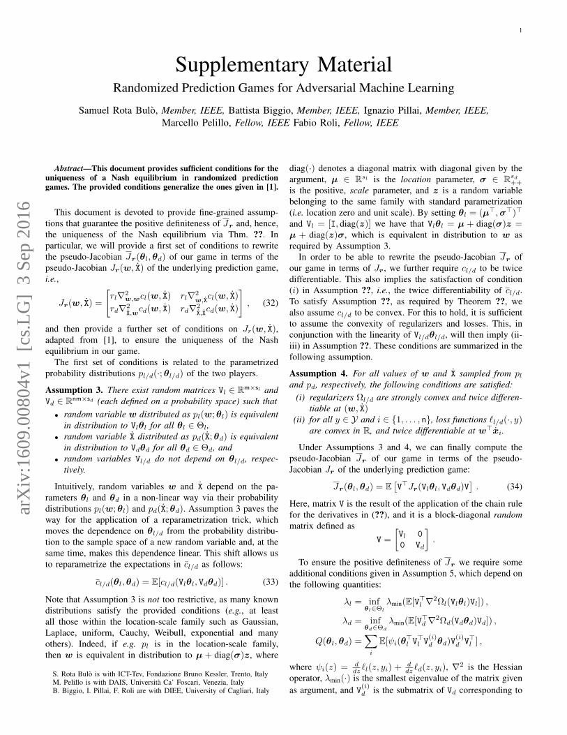
1
Supplementary MaterialRandomized Prediction Games for Adversarial Machine Learning
Samuel Rota Bulo, Member, IEEE, Battista Biggio, Member, IEEE, Ignazio Pillai, Member, IEEE,Marcello Pelillo, Fellow, IEEE Fabio Roli, Fellow, IEEE
Abstract—This document provides sufficient conditions for theuniqueness of a Nash equilibrium in randomized predictiongames. The provided conditions generalize the ones given in [1].
This document is devoted to provide fine-grained assump-tions that guarantee the positive definiteness of Jr and, hence,the uniqueness of the Nash equilibrium via Thm. ??. Inparticular, we will provide a first set of conditions to rewritethe pseudo-Jacobian Jr(θl,θd) of our game in terms of thepseudo-Jacobian Jr(w, X) of the underlying prediction game,i.e.,
Jr(w, X) =
[rl∇2
w,wcl(w, X) rl∇2w,X
cl(w, X)
rd∇2X,w
cd(w, X) rd∇2X,Xcd(w, X)
], (32)
and then provide a further set of conditions on Jr(w, X),adapted from [1], to ensure the uniqueness of the Nashequilibrium in our game.
The first set of conditions is related to the parametrizedprobability distributions pl/d(·;θl/d) of the two players.
Assumption 3. There exist random matrices Vl ∈ Rm×sl andVd ∈ Rnm×sd (each defined on a probability space) such that• random variable w distributed as pl(w;θl) is equivalent
in distribution to Vlθl for all θl ∈ Θl,• random variable X distributed as pd(X;θd) is equivalent
in distribution to Vdθd for all θd ∈ Θd, and• random variables Vl/d do not depend on θl/d, respec-
tively.
Intuitively, random variables w and X depend on the pa-rameters θl and θd in a non-linear way via their probabilitydistributions pl(w;θl) and pd(X;θd). Assumption 3 paves theway for the application of a reparametrization trick, whichmoves the dependence on θl/d from the probability distribu-tion to the sample space of a new random variable and, at thesame time, makes this dependence linear. This shift allows usto reparametrize the expectations in cl/d as follows:
cl/d(θl,θd) = E[cl/d(Vlθl, Vdθd)] . (33)
Note that Assumption 3 is not too restrictive, as many knowndistributions satisfy the provided conditions (e.g., at leastall those within the location-scale family such as Gaussian,Laplace, uniform, Cauchy, Weibull, exponential and manyothers). Indeed, if e.g. pl is in the location-scale family,then w is equivalent in distribution to µ + diag(σ)z, where
S. Rota Bulo is with ICT-Tev, Fondazione Bruno Kessler, Trento, ItalyM. Pelillo is with DAIS, Universita Ca’ Foscari, Venezia, ItalyB. Biggio, I. Pillai, F. Roli are with DIEE, University of Cagliari, Italy
diag(·) denotes a diagonal matrix with diagonal given by theargument, µ ∈ Rsl is the location parameter, σ ∈ Rsd++
is the positive, scale parameter, and z is a random variablebelonging to the same family with standard parametrization(i.e. location zero and unit scale). By setting θl = (µ>,σ>)>
and Vl = [I, diag(z)] we have that Vlθl = µ + diag(σ)z =µ + diag(z)σ, which is equivalent in distribution to w asrequired by Assumption 3.
In order to be able to rewrite the pseudo-Jacobian Jr ofour game in terms of Jr, we further require cl/d to be twicedifferentiable. This also implies the satisfaction of condition(i) in Assumption ??, i.e., the twice differentiability of cl/d.To satisfy Assumption ??, as required by Theorem ??, wealso assume cl/d to be convex. For this to hold, it is sufficientto assume the convexity of regularizers and losses. This, inconjunction with the linearity of Vl/dθl/d, will then imply (ii-iii) in Assumption ??. These conditions are summarized in thefollowing assumption.
Assumption 4. For all values of w and X sampled from pland pd, respectively, the following conditions are satisfied:
(i) regularizers Ωl/d are strongly convex and twice differen-tiable at (w, X)
(ii) for all y ∈ Y and i ∈ 1, . . . , n, loss functions `l/d(·, y)are convex in R, and twice differentiable at w>xi.
Under Assumptions 3 and 4, we can finally compute thepseudo-Jacobian Jr of our game in terms of the pseudo-Jacobian Jr of the underlying prediction game:
Jr(θl,θd) = E[V>Jr(Vlθl, Vdθd)V
]. (34)
Here, matrix V is the result of the application of the chain rulefor the derivatives in (??), and it is a block-diagonal randommatrix defined as
V =
[Vl 0
0 Vd
].
To ensure the positive definiteness of Jr we require someadditional conditions given in Assumption 5, which depend onthe following quantities:
λl = infθl∈Θl
λmin(E[V>l ∇2Ωl(Vlθl)Vl]) ,
λd = infθd∈Θd
λmin(E[V>d ∇2Ωd(Vdθd)Vd]) ,
Q(θl,θd) =∑
i
E[ψi(θ>l V>l V
(i)d θd)V
(i)d V>l ] ,
where ψi(z) = ddz `l(z, yi) + d
dz `d(z, yi), ∇2 is the Hessianoperator, λmin(·) is the smallest eigenvalue of the matrix givenas argument, and V
(i)d is the submatrix of Vd corresponding to
arX
iv:1
609.
0080
4v1
[cs
.LG
] 3
Sep
201
6
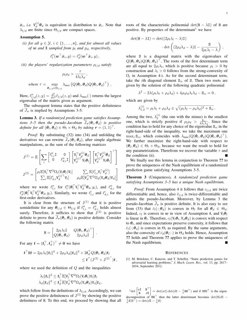
2
xi, i.e. V(i)d θd is equivalent in distribution to xi. Note that
λl/d are finite since Θl/d are compact spaces.
Assumption 5.(i) for all y ∈ Y , i ∈ 1, . . . , n, and for almost all values
of w and X sampled from pl and pd, respectively,
`′′l (w>xi, y) = `′′d(w>xi, y) ,
(ii) the players’ regularization parameters ρl/d satisfy
ρlρd >τ
4λlλd,
where τ = supθl/d∈Θl/d
λmax(Q(θl,θd)Q(θl,θd)
>) ,
Here, `′′l/d(z, y) = d2
dz2 `l/d(z, y) and λmax(·) returns the largesteigenvalue of the matrix given as argument.
The subsequent lemma states that the positive definitenessof Jr is implied by Assumptions 3-5:
Lemma 3. If a randomized prediction game satisfies Assump-tions 3–5 then the pseudo-Jacobian Jr(θl,θd) is positivedefinite for all (θl,θd) ∈ Θl ×Θd by taking r = (1, 1)>.
Proof: By substituting (32) into (34) and unfolding thederivatives we can rewirte Jr(θl,θd), after simple algebraicmanipulations, as the sum of the following matrices
J(1) = E
∑
i
[`′′l,iI 0
0 `′′d,iI
] [V>l V
(i)d θd
V(i)>d Vlθl
][V>l V
(i)d θd
V(i)>d Vlθl
]>
J(2) =
[ρlE[V>l ∇2Ωl(Vlθl)Vl]
∑i E[`′l,iV
>l V
(i)d ]∑
i E[`′d,iV(i)>d Vl] ρdE[V>d ∇2Ωd(Vdθd)Vd]
]
where we wrote `′′l,i for `′′l (θ>l V>l V
(i)d θd, yi), and `′′d,i for
`′′d(θ>l V>l V
(i)d θd, yi). Similarly, we wrote `′l,i and `′d,i for the
first-order derivatives.It is clear from the structure of J(1) that it is positive
semidefinite for any θl/d ∈ Θl/d if `′′l,i = `′′d,i holds almostsurely. Therefore, it sufficies to show that J(2) is positivedefinite to prove that Jr(θl,θd) is positive definite. Considerthe following matrix
H =
[2ρlλlI Q(θl,θd)
>
Q(θl,θd) 2ρdλdI
].
For any t = (t>l , t>d )> 6= 0 we have
t>Ht = 2ρlλl‖tl‖2 + 2ρdλd‖td‖2 + 2t>d Q(θl,θd)tl
≤ t>(J(2) + J(2)>)t ,
where we used the definition of Q and the inequalities
λl‖tl‖2 ≤ t>l E[V>l ∇2Ωl(Vlθl)Vl]tl
λd‖td‖2 ≤ t>d E[V>d ∇2Ωd(Vdθd)Vd]td ,
which follow from the definitions of λl/d. Accordingly, we canprove the positive definiteness of J(2) by showing the positivedefinitness of H. To this end, we proceed by showing that all
roots of the characteristic polinomial det(H − λI) of H arepositive. By properties of the determinant1 we have
det(H− λI) = det((2ρlλl − λ)I)
· det
((2ρdλd − λ)I− S
2ρlλl − λ
),
where S is a diagonal matrix with the eigenvalues ofQ(θl,θd)Q(θl,θd)
>. The roots of the first determinant termare all equal to 2ρlλl, which is positive because ρl > 0 byconstruction and λl > 0 follows from the strong-convexity ofΩl in Assumption 4-i. As for the second determinant term,take the ith diagonal element Sii of S. Then two roots aregiven by the solution of the following quadratic polinomial
λ2 − 2λ(ρlλl + ρdλd) + 4ρlρdλlλd − Sii = 0 ,
which are given by
λ(i)1,2 = ρlλl + ρdλd ±
√(ρlλl − ρdλd)2 + Sii .
Among the two, λ(i)2 (the one with the minus) is the smallest
one, which is strictly positive if ρlρd > Sii4λlλd
. Since thecondition has to hold for any choice of the eigenvalue Sii in theright-hand-side of the inequality, we take the maximum onemaxi Sii, which coincides with λmax(Q(θl,θd)Q(θl,θd)
>).We further maximize the right-hand-side with respect to(θl,θd) ∈ Θl × Θd, because we want the result to hold forany parametrization. Therefrom we recover the variable τ andthe condition (ii).
We finally use this lemma in conjunction to Theorem ?? toprove the uniqueness of the Nash equilibrium of a randomizedprediction game satisfying Assumptions 3-5.
Theorem 3 (Uniqueness). A randomized prediction gamesatisfying Assumptions 3–5 has a unique Nash equilibrium.
Proof: From Assumption 4 it follows that cl/d are twicedifferentiable and, hence, also cl/d is twice-differentiable andadmits the pseudo-Jacobian. Moreover, by Lemma 3 thepseudo-Jacobian Jr is positive definite. It is also easy to seefrom (33) that cl(·;θd) is convex in Θl for all θd ∈ Θd.Indeed, cl is convex in w in view of Assumption 4, and Vlθlis linear in θl. Therefore, cl(Vlθl, Vdθd) is convex with respectto θl, and since expectations preserve convexity, it follows thatcl(·;θd) is convex in Θl as required. By the same arguments,also the convexity of cd(θl; ·) in Θd holds. Hence, Assumption?? holds and Theorem ?? applies to prove the uniqueness ofthe Nash equilibrium.
REFERENCES
[1] M. Bruckner, C. Kanzow, and T. Scheffer, “Static prediction games foradversarial learning problems,” J. Mach. Learn. Res., vol. 13, pp. 2617–2654, September 2012.
1det
[aI B>
B dI
]= det(aI) det(dI − 1
aBB>) and if USU> is the eigen-
decomposition of BB> then the latter deterimnant becomes det(U(dI −1aS)U>) = det(dI− 1
aS)