range-wide network of priority areas for greater sage ... · greater sage-grouse—a design for...

U.S. Department of the InteriorU.S. Geological Survey

Open-File Report 2015–1158

Prepared in cooperation with the U.S. Fish and Wildlife Service

Range-Wide Network of Priority Areas for Greater Sage-Grouse—A Design for Conserving Connected Distributions or Isolating Individual Zoos?

U.S. Department of the Interior U.S. Geological Survey


By Michele R. Crist, Steven T. Knick, and Steven E. Hanser

Prepared in cooperation with the U.S. Fish and Wildlife Service


U.S. Department of the Interior SALLY JEWELL, Secretary

U.S. Geological Survey Suzette M. Kimball, Acting Director

U.S. Geological Survey, Reston, Virginia: 2015

For more information on the USGS—the Federal source for science about the Earth, its natural and living resources, natural hazards, and the environment—visit http://www.usgs.gov/ or call 1–888–ASK–USGS (1–888–275–8747).

For an overview of USGS information products, including maps, imagery, and publications, visit http://www.usgs.gov/pubprod/.

Any use of trade, firm, or product names is for descriptive purposes only and does not imply endorsement by the U.S. Government.

Although this information product, for the most part, is in the public domain, it also may contain copyrighted materials as noted in the text. Permission to reproduce copyrighted items must be secured from the copyright owner.

Suggested citation: Crist, M.R., Knick, S.T., and Hanser, S.E., 2015, Range-wide network of priority areas for greater sage-grouse—A design for conserving connected distributions or isolating individual zoos?: U.S. Geological Survey Open-File Report 2015-1158, 34 p., http://dx.doi.org/10.3133/ofr20151158.

ISSN 2331-1258 (online)

iii

Contents Abstract ......................................................................................................................................................... 1 Introduction .................................................................................................................................................... 1 Description of Study Area .............................................................................................................................. 3 Methods ......................................................................................................................................................... 5

Priority Areas as a Spatial Network ............................................................................................................ 5 Movement Potential among Priority Areas ................................................................................................. 6 Network Analysis ..................................................................................................................................... 10 Relative Isolation ...................................................................................................................................... 10

Results ......................................................................................................................................................... 11 Priority Areas as a Spatial Network .......................................................................................................... 11 Connectivity among Priority Areas ........................................................................................................... 14 Relative Isolation ...................................................................................................................................... 16

Discussion ................................................................................................................................................... 16 Priority Areas as a Spatial Network .......................................................................................................... 16 Connectivity among Priority Areas ........................................................................................................... 17 Relative Isolation ...................................................................................................................................... 18 Synthesis and Application ........................................................................................................................ 18

Acknowledgments ....................................................................................................................................... 19 References Cited ......................................................................................................................................... 20 Appendix A. Crosswalk Table Depicting Priority Area Identifiers, U.S. Fish and Wildlife Service Unique Identifiers, Sage-Grouse Population Name, and Management Zone ........................................................... 24 Appendix B. Centrality Results for Degree and Betweenness Metrics for Each Priority Area ...................... 30

Figures Figure 1. Study area and designated priority areas across the sage-grouse range in western North America represented as a network of nodes and links. ........................................................................ 4 Figure 2. Habitat similarity index (HSI) values for greater sage-grouse across their historical range. .......... 9 Figure 3. Priority area importance and connectivity for betweenness centrality and ranked across the network ........................................................................................................................................................ 12 Figure 4. Relative contribution of each priority area to range-wide cumulative percent betweenness centrality ...................................................................................................................................................... 13 Figure 5. Cumulative distribution of each priority area’s contribution to total betweenness centrality ......... 14 Figure 6. Relative isolation of priority areas based on estimated potential for sage-grouse movement (Circuitscape; McRae and Shah, 2008) ....................................................................................................... 15

Tables Table 1. Partitions (k) in a Mahalanobis D2 model describing ecological minimums for the range-wide distribution of greater sage-grouse ................................................................................................................ 8 Table 2. Summary statistics calculated for degree and betweenness centrality, and effective resistance and maximum current densities from Circuitscape (McRae and others, 2008)........................... 11

iv

Conversion Factors International System of Units to Inch/Pound

Multiply By To obtain

Length kilometer (km) 0.6214 mile (mi)

Area hectare (ha) 2.471 acre

square hectometer (hm2) 2.471 acre

square kilometer (km2) 247.1 acre

square kilometer (km2) 0.3861 square mile (mi2) Vertical coordinate information is referenced to the North American Vertical Datum of 1988 (NAVD 88).

Horizontal coordinate information is referenced to the North American Datum of 1983 (NAD 83).

Elevation, as used in this report, refers to distance above the vertical datum.

1


By Michele R. Crist, Steven T. Knick, and Steven E. Hanser

Abstract The network of areas delineated in 11 Western States for prioritizing management of

greater sage-grouse (Centrocercus urophasianus) represents a grand experiment in conservation biology and reserve design. We used centrality metrics from social network theory to gain insights into how this priority area network might function. The network was highly centralized. Twenty of 188 priority areas accounted for 80 percent of the total centrality scores. These priority areas, characterized by large size and a central location in the range-wide distribution, are strongholds for greater sage-grouse populations and also might function as sources. Mid-ranking priority areas may serve as stepping stones because of their location between large central and smaller peripheral priority areas. The current network design and conservation strategy has risks. The contribution of almost one-half (n = 93) of the priority areas combined for less than 1 percent of the cumulative centrality scores for the network. These priority areas individually are likely too small to support viable sage-grouse populations within their boundary. Without habitat corridors to connect small priority areas either to larger priority areas or as a clustered group within the network, their isolation could lead to loss of sage-grouse within these regions of the network.

Introduction Greater sage-grouse (Centrocercus urophasianus; hereinafter, sage-grouse) is an endemic

Galliform to arid and semiarid sagebrush (Artemisia spp.) landscapes of Western North America (Schroeder and others, 1999). Sage-grouse currently occupy approximately one-half of their presettlement habitat distribution and have recently received much attention for their long-term population declines (Schroeder and others, 2004; Garton and others, 2011). The U.S. Fish and Wildlife Service listed sage-grouse as a candidate species under the Endangered Species Act in 2010 concluding that protection was warranted although immediate conservation actions were precluded due to other higher priority species (U.S. Fish and Wildlife Service, 2010). Broad-scale habitat loss and fragmentation from synergistic cycles of wildfire and conversion to invasive plant communities as well as from human land use is the primary cause of population declines (Knick and Connelly, 2011). The most pressing challenge to long-term sage-grouse persistence is conservation of remaining large and intact sagebrush landscapes (Stiver and others, 2006).

2

The U.S. Fish and Wildlife Service, faced with legal challenges for delaying full protection under the Endangered Species Act, is currently reviewing the bird’s status and is scheduled to issue an updated listing decision in September 2015. In an effort to avoid listing, the 11 Western States and Federal management agencies within the sage-grouse range have developed conservation plans embracing the concept of core or priority areas (Priority Areas for Conservation, PACs [U.S. Fish and Wildlife Service, 2013], or equivalent terms designated in individual State agency plans)—allowable spatial area of disturbance due to human land use, such as energy development, is tightly regulated and conservation actions are focused in areas with the highest number of sage-grouse and potentially the greatest benefit to the species. Land use is allowed to continue outside of priority areas under normal regulations.

The delineation of an entire species range spanning more than 2 million km2 (excluding the Canadian portion) into a binary division of priority and nonpriority areas may represent one of the largest experiments in conservation reserve design for a single species. Individual priority areas range in size from less than 1 to more than 83,000 km2 and encompass the broad spectrum of reserve design paradigms from single large to several small reserves. Although we do not know the minimum area required, the largest priority areas likely can support viable sage-grouse populations completely within their boundaries. However, the smallest priority areas clearly enclose much less than the annual range of a sage-grouse (4–615 km2; Connelly and others, 2011). Much scientific literature addressing conservation reserve design has stressed the importance of the inclusion and protection of habitat connectivity between conservation reserves to ensure individual movements, opportunity to shift habitats when needed, and facilitate genetic exchange (Crooks and Sanjayan, 2006). Therefore, numerous connected priority areas also may be necessary to provide seasonal habitats that can be separated by up to 160 km (Connelly and others, 2011; Smith, 2013). The two primary factors that influence populations, area and isolation (MacArthur and Wilson, 1967; Hanski and Gilpin, 1991; Hanski, 1999), are important metrics in understanding the efficacy of this conservation approach.

We used social network theory and centrality metrics (Moreno, 1932, 1934; Freeman, 1979, 2004) to quantify and understand the potential for the delineated priority areas to function as a connected network to conserve sage-grouse populations. Our objectives were to:

1. Identify high-ranking priority areas within the network based on their location and number of connections to other priority areas,

2. Estimate the ability of other lower ranking priority areas within the network to function as stepping stones for maintaining connectivity among clusters of priority areas, and

3. Model relative isolation among priority areas based on movement potential in their surrounding environment.

3

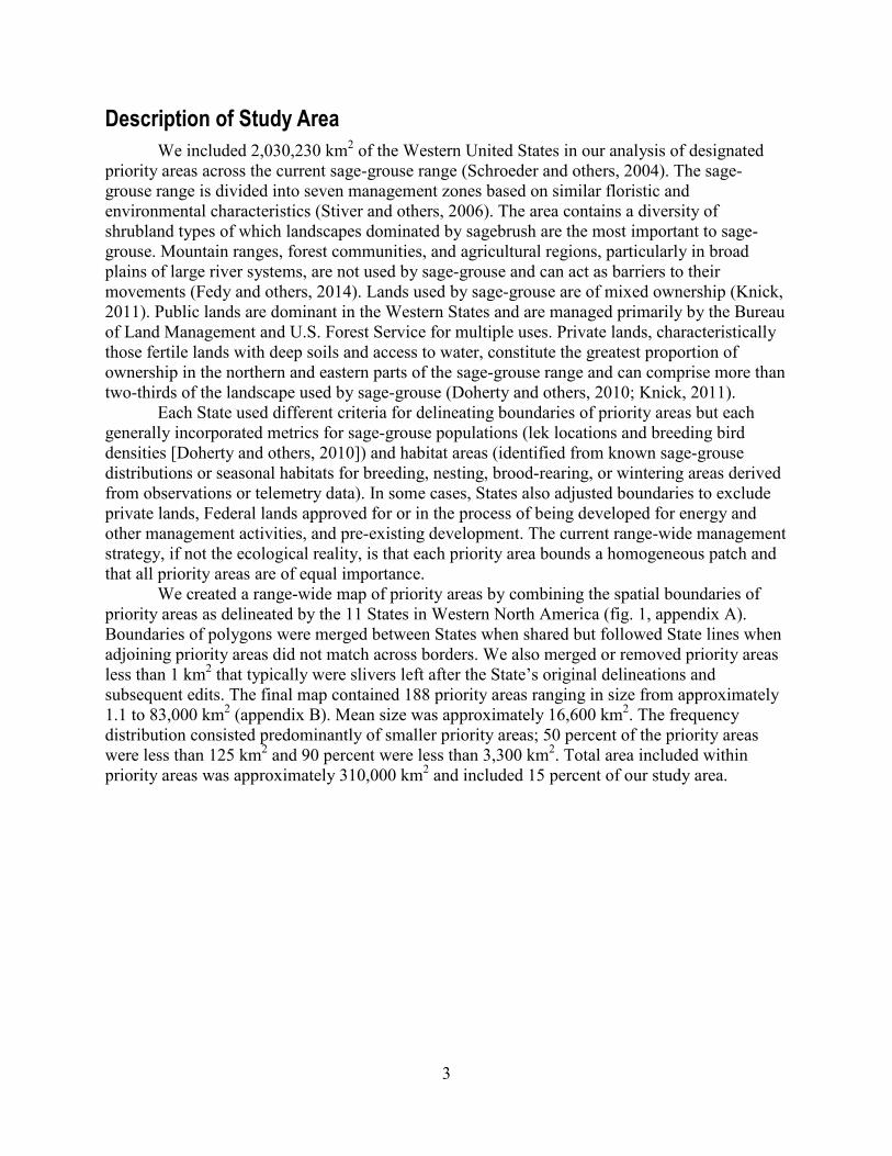
Description of Study Area We included 2,030,230 km2 of the Western United States in our analysis of designated

priority areas across the current sage-grouse range (Schroeder and others, 2004). The sage-grouse range is divided into seven management zones based on similar floristic and environmental characteristics (Stiver and others, 2006). The area contains a diversity of shrubland types of which landscapes dominated by sagebrush are the most important to sage-grouse. Mountain ranges, forest communities, and agricultural regions, particularly in broad plains of large river systems, are not used by sage-grouse and can act as barriers to their movements (Fedy and others, 2014). Lands used by sage-grouse are of mixed ownership (Knick, 2011). Public lands are dominant in the Western States and are managed primarily by the Bureau of Land Management and U.S. Forest Service for multiple uses. Private lands, characteristically those fertile lands with deep soils and access to water, constitute the greatest proportion of ownership in the northern and eastern parts of the sage-grouse range and can comprise more than two-thirds of the landscape used by sage-grouse (Doherty and others, 2010; Knick, 2011).

Each State used different criteria for delineating boundaries of priority areas but each generally incorporated metrics for sage-grouse populations (lek locations and breeding bird densities [Doherty and others, 2010]) and habitat areas (identified from known sage-grouse distributions or seasonal habitats for breeding, nesting, brood-rearing, or wintering areas derived from observations or telemetry data). In some cases, States also adjusted boundaries to exclude private lands, Federal lands approved for or in the process of being developed for energy and other management activities, and pre-existing development. The current range-wide management strategy, if not the ecological reality, is that each priority area bounds a homogeneous patch and that all priority areas are of equal importance.

We created a range-wide map of priority areas by combining the spatial boundaries of priority areas as delineated by the 11 States in Western North America (fig. 1, appendix A). Boundaries of polygons were merged between States when shared but followed State lines when adjoining priority areas did not match across borders. We also merged or removed priority areas less than 1 km2 that typically were slivers left after the State’s original delineations and subsequent edits. The final map contained 188 priority areas ranging in size from approximately 1.1 to 83,000 km2 (appendix B). Mean size was approximately 16,600 km2. The frequency distribution consisted predominantly of smaller priority areas; 50 percent of the priority areas were less than 125 km2 and 90 percent were less than 3,300 km2. Total area included within priority areas was approximately 310,000 km2 and included 15 percent of our study area.

4

Figure 1. Study area and designated priority areas across the sage-grouse range in Western North America represented as a network of nodes and links. Background map is from U.S. Geological Survey National Elevation Data (NED; 2011; http://seamless.usgs.gov).

5

Methods

Priority Areas as a Spatial Network We described the spatial network of priority areas as a graph structured by nodes and

connecting links (Diestel, 2005). To identify adjacencies, we delineated individual polygons around each priority area by creating Thiessen polygons where boundaries encompassed grid cells closest to each priority area relative to all other priority areas. Shared boundaries between Thiessen polygons identified neighboring priority areas. We then added links between each priority area and its neighbor’s centroid. Thus, the network of conservation reserves currently designed for the sage-grouse range was represented by nodes and links across all priority areas (fig. 1).

We used analyses derived from social network theory (Wasserman and Faust, 2004) to identify priority areas that were highly important for connectivity within the range-wide network. Social network theory combines graph theory and centrality indices to characterize network structures by mapping and measuring relationships and flows (links) between people, groups, organizations, computers, and other entities (nodes) (Freeman, 2004; Wasserman and Faust, 2004; Diestel, 2005; Newman, 2010). Quantifying network centrality provides insight into the overall structure, connection, and function of a network, and is considered to be the fundamental characteristic describing a node’s position in a network. Relative importance in social networks is measured by centrality metrics that emphasize number of connections to indicate relative position within the network. Networks can range from highly centralized, dominated by a few highly connected nodes, to more widely dispersed configurations in which connections are equally shared among all nodes.

We used two centrality metrics, degree and betweenness, to assess the relative importance of individual priority areas based on their position and number of connections within the overall range-wide network (Freeman, 1977, 2004; Wasserman and Faust, 2004; Newman, 2010). Relative importance estimated by degree centrality is based simply on number of connections to other nodes in the network; more connections indicate greater influence and a more central position in the network (Erdos and Gallai, 1960; Diestel, 2005). However, a priority area also might be important because its relative position connects clusters or groups of priority areas located in close proximity. Betweenness centrality quantifies the number of times a node acts as a bridge along the shortest path between two other nodes, thus indicating its importance in maintaining the network (Freeman, 1977; Freeman and others, 1991; Estrada, 2007; Brandes, 2008; González-Pereira and others, 2010). Nodes with high scores of betweenness centrality represent the primary foundation of the network’s structure because a disproportionately high number of the shortest pathways go through them. These nodes funnel movement not only from adjacent nodes but also from nodes that could be located far away in the landscape (Bodin and Norberg, 2007).

6

Movement Potential among Priority Areas Connections in ecological networks are not without dimensions (as in social networks)

but rather have a distance and environmental cost to move between nodes (Bunn and others, 2000; McRae and others, 2008; Carroll and others, 2012; LaPointe and others, 2013). To assess the relative importance of priority areas, we needed to combine number of connections with the ability to traverse the interstitial landscape matrix.

We calibrated movement potential by sage-grouse through the landscape by mapping a model of ecological minimum requirements (Knick and others, 2013). Sage-grouse may perceive a landscape quite differently when moving within a range, moving between seasonal ranges, or when dispersing. Similarly, connectivity for individual movements obtained from telemetry data might be different than connectivity derived from genetic information. For our study, we made the basic assumption that movement would be more likely in suitable environments that could be modeled across the entire range.

An ecological minimum, in concept, represents a multivariate construct of the basic requirements for a species. The model was developed from 23 variables describing land cover, fire history (area burned from 1980 to 2013), terrain (topographic accessibility [Sappington and others, 2007]), climate, edaphic, and anthropogenic features measured at our minimum mapping unit of 1-km2 resolution across the sage-grouse range. Land-cover variables consisted of combined Landfire Existing Vegetation Type (http://www.landfire.gov/; Rollins, 2009) for big sagebrush, low sagebrush, salt desert shrub, exotic grassland, native grassland, pinyon-juniper woodland, conifer forest, and riparian associations. Climate variables were obtained from the PRISM Climate Group (Daly and others, 2004; Oregon State University, 2011) measured from 1998 to 2010 and included mean annual maximum and minimum temperatures, and mean annual precipitation. We described soils using available water capacity, salinity, and depth to rock (U.S. Department of Agriculture, 2011). Anthropogenic features included agriculture and development land cover (http://www.landfire.gov/), transmission lines, tall structures (communication towers, wind towers), roads, pipelines, and oil and gas wells. We produced a smoothed, continuous surface for most variables by averaging individual cell values within a 5-km radius moving window. We used mapped values for soils, which were in vector format, measured at the center of each 1-km grid cell in the map.

We derived estimates of the ecological minimums using a partitioned Mahalanobis D2 model of presence only data (Dunn and Duncan, 2000; Rotenberry and others, 2002). Lek (breeding area) locations were used to indicate presence for a previous model of sage-grouse ecological minimums across their western range (Knick and others, 2013). However, we did not have permission to use lek data from all States across the sage-grouse range. Therefore, we assumed that the priority areas delineated by States captured higher quality habitat than occurred outside, despite having some areas excluded because of ownership or forecasted disturbance, and a large proportion of the sage-grouse population. We randomly selected 1,669 points within individual priority areas as presence data and extracted values for corresponding variables to calibrate models. Total number of presence points was obtained by proportional area expansion to the eastern part of the sage-grouse range after an initial 1,000 point random sample in a preliminary comparison of results from priority areas compared to the lek-based map in our previous study of the western range (Knick and others, 2013). We then performed a principal components analysis on 1,000 iterative samples created by bootstrapping the calibration data. The final model was created by subsequently averaging the PCA output after correcting for sign ambiguity (Bro and others, 2008) across all iterations.

7

We evaluated model performance from the area under the curve (AUC) for a receiver operating characteristic (ROC) to assess sensitivity (fraction of habitat points correctly classified) and specificity (fraction of non-habitat points predicted as habitat) (Fielding and Bell, 1997). To generate presence data, we overlaid the 100 percent sage-grouse breeding densities (Doherty and others, 2010) representing spatial locations of all known sage-grouse breeding sites with our map of ecological minimums and selected all values that fell within the density boundaries. For absence data, we selected all values that fell outside of the breeding density boundaries. To calculate the AUC, we randomly sampled 5,000 presence points and 20,000 absence points. We also created a null presence/absence dataset by randomly sampling 20,000 points 1,000 times from the ecological minimums map. For each iteration, we divided the resulting sample into two datasets (null presence and null absence) based on a relatively equal proportion of the total rows and columns. We then sampled 10,000 points from each of the two datasets and computed a mean AUC score and distribution from all null samples. Means and distributions for model and null AUC scores then were used in a t-test for significance.

Principal component partition 14 met our criteria of having an eigenvalue <1, a relative difference in eigenvalues among adjacent partitions (table 1), performance against evaluation data (AUC = 0.80; null AUC = 0.50; 95% CI = 0.49 and 0.50; t-test between the null AUC and true AUC = -3,775.0; p << 0.001), and our subjective assessment of mapped results from different model partitions. We rescaled the mapped output to range continuously from 0 to 1 based on a χ2 distribution of the D2 distance; a value of 1 indicated environmental conditions identical to the mean vector of ecological minimum requirements, whereas a value near 0 indicated very dissimilar conditions (fig. 2).

We used circuit theory (McRae and others, 2008) to model movement pathways between all priority areas across our network. We assumed that sage-grouse moved more readily through areas meeting their ecological minimum requirements and used a scaled inverse of our mapped scores as a resistance surface (McRae and others, 2008; Spear and others, 2010; Beier and others, 2011; Zeller and others, 2012). Our resistance surface was calculated by multiplying habitat values by 100 and using the following function: ((habitat value – maximum habitat value) * -1) + minimum habitat value). Resistance values ranged from 1, representing the lowest resistance/highest habitat value, to 100 (high resistance/lowest habitat value). We ran Circuitscape (Circuitscape version 4.0, http://www.circuitscape.org; McRae and Shah, 2008) using the pairwise mode to calculate connectivity between all pairs of priority areas. We treated priority areas as focal patches instead of individual nodes in the modeling process: evaluating habitat pathways from priority area polygon boundaries rather than nodes captured the influence of priority area structure and size in influencing current flow. Effective resistance distances, the relative distance that incorporates the resistance to a species movements across a heterogeneous landscape and used as an estimate of connectivity, were calculated iteratively between all priority area pairs and maps of current densities. We calculated electric current flowing through the resistance landscape between each pair to produce cumulative and maximum current densities across all pair-wise combinations. Our approach thus incorporated multiple dispersal pathways and landscape heterogeneity.

8

Table 1. Partitions (k) in a Mahalanobis D2 model describing ecological minimums for the range-wide distribution of greater sage-grouse.

Partition (k) Eigenvalue 1 3.18 2 2.89 3 1.87 4 1.76 5 1.68 6 1.42 7 1.31 8 0.99 9 0.96

10 0.93 11 0.85 12 0.80 13 0.76 14 0.63 15 0.59 16 0.49 17 0.44 18 0.40 19 0.34 20 0.32 21 0.24 22 0.14 23 0.04

9

Figure 2. Habitat similarity index (HSI) values for greater sage-grouse across their historical range. HSI values represent the relationship of environmental values at map locations to the multivariate mean vector of minimum requirements for sage-grouse defined by land cover, anthropogenic variables, soil, topography, and climate.

10

Network Analysis We applied the effective resistance distances calculated between priority areas to our

priority area network. We exported the attribute table of our line network shapefile and built a matrix based on priority area IDs, where “0” was assigned to indicate non-adjacency for a priority area pair (where the two priority areas are not linked in the network), and a “1” indicates adjacency (priority area pairs are linked). We assigned the resulting pair-wise effective resistance distances as a cost between adjacent priority areas in the matrix to all priority pair adjacencies labeled with a “1”. For example, a low effective resistance distance represents a relative capability for sage-grouse movements between the priority area pair based on similarity to habitats within priority areas. We rebuilt our node and link network from our matrices using the igraph package in R (Csardi and Nepusz, 2006; R Core Team, 2013) to calculate centrality. Links connecting adjacent priority areas represent a relation between the priority areas based on the effective resistance distance. The final graph represented the priority area network’s spatial structure of connectivity.

We calculated our centrality metrics, degree and betweenness, using the igraph package and computed summary statistics of our centrality results using R (Csardi and Nepusz, 2006; R Core Team, 2013). We also computed a cumulative distribution curve for resulting betweenness centrality values and used the incremental contribution by each priority areas to assess its contribution to overall network centrality. We used the distribution to rank and identify central priority areas that contribute the most in maintaining a connected network and to identify priority areas that function as stepping stones in promoting connectivity to the central priority areas.

Relative Isolation Our final objective was to model the relative isolation of priority areas across the

historical range of sage-grouse. Results from Circuitscape were used to map habitat linkages among all priority areas and identify clusters of connected priority areas within our network. Circuit theory is advantageous for quantifying connectivity in this manner because of its ability to simultaneously evaluate the combined contributions of multiple pathways to dispersal in heterogeneous landscapes, and identify areas important for connectivity conservation (McRae, 2006; McRae and others, 2008). We used visual observations of the maximum current densities and computed effective resistance distances resulting from Circuitscape to identify areas where habitat connectivity is high or low between priority areas. We chose to evaluate the maximum current density map because maximum values help to remove the confounding effects of network configuration (halo effect) in the Circuitscape results. Again, greater connectivity among priority areas was reflected by a larger number of connected pathways and lower effective resistance distance values (McRae and Shah, 2008; McRae and others, 2008). We also visually identified locations of high current densities that may function as bottlenecks (pinch points) to sage-grouse movements where alternative pathways are not available (McRae and others, 2008). These locations may represent conservation priorities for sage-grouse because their loss may disrupt connectivity among the priority area network.

11

Results Priority Areas as a Spatial Network

Average number of connections from each priority area to adjacent neighbors averaged 11 and ranged from 2 to 50 (fig. 3). Betweenness centrality scores ranged from 0 to 11,414 (table 2; appendix B); the average betweenness centrality was 475 (table 2), indicating that most priority areas were contributing little to the range-wide centrality. The largest priority area (Priority Area ID 48), which combined individual State polygons in northeastern Oregon, western California, northern Nevada, southern Idaho, and western Utah, exhibited the highest number of adjacent neighbors (n = 50) and highest betweenness centrality value, signifying its importance in connecting the network.

Twenty priority areas explained 80 percent of the total betweenness centrality value and were likely the central priority areas for maintaining a connected reserve network (fig. 4). Two priority areas that exhibited the highest betweenness centrality scores and explained 20 percent of total centrality were the largest single polygon (Priority Area ID 48) and a priority area centrally located in Wyoming (Priority Area ID 110). Priority areas that were within the 80–99 percent cumulative distribution scored lower in centrality compared to the central priority areas but may still contribute largely by functioning as stepping stones maintaining connections across the most central 20 priority areas. These priority areas typically were located between the highest- and lowest-scoring priority areas, mid-sized in area, and were distributed across the entire range rather than having a more central location.

Ninety-three priority areas that scored a 0 for betweenness centrality were characterized by small size (averaging approximately 350 km2), and were either isolated between large priority areas where the shape of the surrounding large priority areas limited the number of connections, or were located on the periphery of the range. Although these small priority areas were not central in maintaining the overall network, most scored low in the effective resistance distance results (figs. 4 and 5; appendix B) indicating high connectivity to their neighboring priority areas.

Table 2. Summary statistics calculated for degree and betweenness centrality, and effective resistance and maximum current densities from Circuitscape (McRae and others, 2008).

Priority Areas Mean Minimum Maximum

Distance between Priority Areas (km) 99.3 2.7 843.3 Degree Centrality Metric 10.6 2.0 50.0

Betweenness Centrality Metric 475 0 11,414

Priority Area Effective Resistance 4.4 <0.1 35.8

Maximum Current Densities 0.1 0.0 1.0

12

Figure 3. Priority area importance and connectivity for betweenness centrality and ranked across the network. Potential for sage-grouse movements was estimated between priority areas and used to determine each priority area’s centrality based on the number of movement pathways available between priority areas. Current densities were displayed using a histogram equalize stretch.

13

Figure 4. Relative contribution of each priority area to range-wide cumulative percent betweenness centrality. Priority area colors in map correspond with figure 5.

14

Figure 5. Cumulative distribution of each priority area’s contribution to total betweenness centrality. Graph colors correspond to mapped priority areas in figure 4.

Connectivity among Priority Areas Movement potential, estimated by Circuitscape current densities (fig. 6), coupled with the

relatively low mean for priority area effective resistance distance (mean = 4.4; table 2) indicated a high degree of connectivity across the network characterized by numerous and multiple pathways between most of the priority areas. The map reflecting maximum current densities highlighted areas of high current flow between priority areas that may be important habitat linkages (pinch points). Their loss may result in disconnections across the entire network or result in the use of less efficient (more costly) habitat pathways connecting priority areas (fig. 6). A number of linkages have portions of high current densities that depict pinch points where connectivity is high but constrained due to either natural or anthropogenic barriers to sage-grouse movements surrounding the pinch points. Our map of maximum current densities also highlighted priority area clusters where current flow was high between priority areas and low surrounding a group of priority areas.

15

Figure 6. Relative isolation of priority areas based on estimated potential for sage-grouse movement (Circuitscape; McRae and Shah, 2008). Inverted HSI values were used as a measure of landscape resistance. Six clusters of priority areas are circled where connectivity between priority areas was high in comparison to surrounding environment. High to medium current densities represent pinch points.

16

Relative Isolation Low current densities highlighted areas where habitat quality was more fragmented or

where barriers for sage-grouse movements may exist. Mean maximum current density across the study area was low (mean = 0.1; table 2) because the study area included large expanses for high elevation mountain ranges, forested communities, highly populated areas, agriculture development, and other areas of low habitat value for sage-grouse that composed a large portion of our study area. For example, the Snake River Plain in southern Idaho, which contains Interstate 84 and large areas of developed private lands, may function as a barrier for sage-grouse movements between two adjoining priority areas. The Snake River Plain also has experienced significant areas of cheatgrass (Bromus tectorum) invasions and recent fire activity resulting in higher habitat loss and fragmentation in comparison to other regions across the historical range.

Discussion

The strategy currently implemented for conserving greater sage-grouse is based on designated priority areas in each of the 11 States across its range (U.S. Fish and Wildlife Service, 2013). Focusing conservation actions on a relatively small (<15 percent) total area containing a large proportion of the range-wide population can have the greatest benefit with limited resources. However, continued management under normal regulations in regions surrounding priority areas can potentially lead to a spatially disjunct set of areas that retain the characteristics necessary to sustain sage-grouse populations. We assumed that the priority areas serve as a system of reserves and function within the context of island biogeography theory (MacArthur and Wilson, 1967; Wiens, 1997).

We used two primary factors, size and connectivity of priority areas, to understand how this network functions. We ranked priority areas for their relative importance within the network and identified important habitat linkages that may help maintain connected sage-grouse populations across their range. However, our approach was a simple metric based on a social theory relating importance to number of connections. The critical component to assessing viability is not just size of priority area and number of connections but how individuals are linked together to function as a viable population.

Priority Areas as a Spatial Network Centrality measures derived from social network theory provided an interpretable

analysis for characterizing the importance of priority areas within a network. Centrality measures also produced a ranking metric for identifying key areas to conserve to minimize network connectivity loss (Freeman, 2004; Blazquez-Cabrera and others, 2014). A highly centralized network is dominated by one or a few very central nodes. If these nodes are removed, the network may quickly fragment into unconnected sub-networks by isolating individual or clusters of nodes. In contrast, a less centralized network might be more resilient because many links or nodes can fail while allowing the remaining nodes to remain connected through other network paths.

17

High centrality scores for 20 of 188 priority areas indicated that the network was highly centralized. Highly ranked priority areas were characterized by large size, a more central spatial location within the network, and were surrounded by many other priority areas of various sizes. The highest ranked priority area (Priority Area ID 48) was the largest and most centrally located in the network. Large size also correlates with longer boundaries that allow for more dispersal opportunity with adjacent priority areas. Similarly, a central position in the network facilitates movement to reach numerous other priority areas, thus increasing overall connectivity across the network. Loss or fragmentation of these large priority areas, or their associated connections, would have a disproportionally large influence across the entire network. Delineating priority areas with these characteristics may be important in further conservation strategies because they play a strong role in the range-wide network connectivity.

Approximately 80 percent of the priority areas scored betweenness centrality values of (near) zero despite being well-connected to surrounding priority areas. These priority areas generally were smaller and were distributed across the network surrounding the central larger priority areas. Although these individual priority areas were small, their total area contained a large amount of the habitat across the entire sage-grouse range. Their size and location likely allows them to function as stepping stones and may be critical for individuals moving from larger neighboring priority areas needed to maintain smaller sage-grouse populations (Bodin and others, 2006; Saura and others, 2014).

Connectivity among Priority Areas Maintaining connectivity by conserving habitat between separated populations or

reserves is an important strategy to mitigate against impacts of land-use change. Landscape connectivity is often assessed in the form of least-cost paths, corridors, and graph networks to identify critical habitat connections where, if severed, could potentially isolate populations (Bunn and others, 2000; Urban and Keitt, 2001; LaPoint and others, 2013). Our primary objective was to evaluate the capability of the network of priority areas to serve as a connected reserve network for sage-grouse. To do that, we also needed to produce the first range-wide landscape-scale analysis to quantify habitat quality and connectivity across their range. This approach, incorporating an effective resistance surface, enhanced our assessment of the priority area network by permitting multiple dispersal pathways and recognizing landscape heterogeneity in estimating movement cost. Our maps highlighted important habitat corridors and pinch points between priority areas that land managers can target for conservation to help ensure sage-grouse seasonal and dispersal movements. These locations also might be considered for future priority areas to ensure connectivity.

We emphasize that the parameters defining connectivity in our study were based on a habitat suitability metric measured at a 1-km2 resolution. The interpretation of connectivity requires an understanding of genetic, individual, and population levels as well as recognizing behavioral differences between seasonal and dispersal movements. Connectivity to maintain genetic diversity might have different requirements than the connectivity necessary to recolonize areas or augment declining populations. Characteristics of sage-grouse dispersal are relatively unknown (Connelly and others, 2011); patterns from telemetry, satellite, and genetic studies would provide valuable information in assessing landscape-scale connectivity for conservation planning.

18

Relative Isolation The cost of movement across a landscape is a combined function of distance and

resistance to movement (McRae, 2006). Connectivity, measured by the effective resistance distance, varied widely across the sage-grouse range. Some geographically distant priority areas were highly connected to the network through corridors of low resistance to movement. In contrast, other priority areas in close proximity were disconnected because of resistance created by unsuitable environments.

The formal conservation strategy focused on priority areas did not designate connecting corridors among priority areas, which could effectively isolate priority areas or regions. Therefore, we identified linkages and pinch-points that may be important for sustaining sage-grouse movements among priority areas (Bengtsson and others, 2003; Beier and others, 2011; Dickson and others, 2013; LaPoint and others, 2013). Most techniques for analyzing landscape connectivity identify one primary route based on a least cost pathway that becomes the focus for conservation efforts. Our approach for characterizing connectivity based on a resistance surface and circuit theory allowed for the quantitative and simultaneous evaluation of multiple alternative habitat linkages important for maintaining connected sage-grouse populations (McRae and others, 2008; Knick and others, 2013).

Synthesis and Application The current network of priority areas has many important characteristics for maintaining

sage-grouse populations. This network contained a range of large and small sizes of priority areas that might provide different functions. The structure of the network of priority areas for conserving greater sage-grouse was highly centralized. A relatively few large and more central priority areas accounted for a large proportion of cumulative centrality ranking. These large priority areas likely can self-sustain viable sage-grouse populations because of the large sagebrush regions within their boundaries. Large priority areas also might function as sources to augment adjacent populations, either those in priority areas too small to support persistent sage-grouse populations or in nonpriority areas.

The network also contained connected clusters of priority areas that otherwise might be too small individually to sustain viable populations. For example, a cluster of priority areas in Wyoming were highly connected and centered on one large priority area. A priority area cluster in Montana appears geographically isolated but is highly connected to the Wyoming cluster through habitat linkages in North and South Dakota. High current densities between priority areas in Oregon connect with priority areas across Idaho, Nevada, and California. The Bi-State cluster on the border of Nevada and California was isolated from all other clusters but exhibited a high degree of connectivity among the priority areas within it. Although our analysis focused on the range-wide network, there is likely a hierarchical system of networks for both priority areas and metapopulations of sage-grouse. These smaller clusters might function independently and an analysis of these smaller clusters as networks might provide important insights into regional centrality and linkages.

19

Designating clustered areas in close proximity is one of the central tenets of reserve design (Diamond, 1975; Williams and others, 2004). Clustering helps to promote frequent dispersal movements for genetic exchange. Clustering also might enhance migration that might rescue declining or isolated populations, allow for seasonal movements, or egress away from areas that have become degraded or lost (Cabeza and Moilanen, 2001). Maintaining connectivity within and among the clusters potentially allows for dispersal to augment declining populations and maintain genetic exchange across the entire network reducing the chance for the creation of isolated or genetically distinct populations in the long-term (Crooks and Sanjayan, 2006).

Priority areas that scored lower in the centrality metrics were mid-sized and widely distributed across the entire range. Their function as stepping stones to reduce overall distance for sage-grouse movements among the central priority areas is an important consideration for sustaining a connected network.

Adopting a range-wide conservation plan for sage-grouse based on a network of priority areas has risks. Different conservation and management priorities among administrative units could disrupt the metapopulation structure leading to greater isolation and potentially initiate or accelerate population declines. Many priority areas share a boundary on State jurisdictional lines and many important habitat linkages presented here occur across State and Federal jurisdictional boundaries. Yet, priorities and land use plans often differ among State and Federal management agencies both within and outside of the proposed priority area structure (Copeland and others, 2014). Understanding the functions of the priority area network and recognizing the importance of connecting corridors can help sustain sage-grouse populations.

Designing reserve networks is challenging because of combined needs to protect the largest habitat or population areas in a landscape, ensure that those areas are close enough to sustain effective dispersal rates, and also ensure that a sufficient number of areas exist so that individual losses can be absorbed within the entire network (Diamond, 1975; Cabeza and Moilanen, 2001; Williams and others, 2004). Our centrality results may help predict impacts to connectivity when priority areas are lost, degraded, or fragmented. Numerous factors, both natural and anthropogenic, make it unlikely that the current network of priority areas can be sustained (Knick and Connelly, 2011). Focusing conservation actions on important and highly connected priority areas and corresponding habitat linkages may help to mitigate future landscape change and enhance the long-term viability of sage-grouse populations.

Acknowledgments Western Association of Fish and Wildlife Agencies within the sage-grouse range

provided spatial data. U.S. Geological Survey provided ancillary support. D.E. Naugle, University of Montana, was responsible for the zoo metaphor. S.L. Phillips, U.S. Geological Survey, reviewed an early draft of the manuscript.

20

References Cited Beier, P., Spencer, W., Baldwin, R., and McRae, B. H., 2011, Best science practices for

developing regional connectivity maps: Conservation Biology, v. 25, p. 879–892. Bengtsson, J., Angelstam, P., Elmqvist, T., Emanuelsson, U., Folke, C., Ihse, M., Moberg, F.,

and Nyström, M., 2003, Reserves, resilience and dynamic landscapes: Ambio, v. 32, p. 389–396.

Blazquez-Cabrera, S., Bodin, Ö., and Saura, S., 2014, Indicators of the impacts of habitat loss on connectivity and related conservation priorities—Do they change when habitat patches are defined at different scales?: Ecological Indicators, v. 60, p. 704–716.

Bodin, Ö., and Norberg, J., 2007, A network approach for analyzing spatially structured populations in fragmented landscapes: Landscape Ecology, v. 22, p. 31–44.

Bodin, Ö., Tengö, M., Norman, A., Lundberg, J., and Elmqvist, T., 2006, The value of small size—Loss of forest patches and ecological thresholds in southern Madagascar: Ecological Applications, v. 16, p. 440–451.

Brandes, U., 2008, On variants of shortest-path betweenness centrality and their generic computation: Social Networks, v. 30, p. 136–145.

Bro, R., Acar, E., and Kolda, T.G., 2008, Resolving the sign ambiguity in the singular value decomposition: Journal of Chemometrics, v. 22, p. 135–140.

Bunn, A.G., Urban, D.L., and Keitt, T.H., 2000, Landscape connectivity—A conservation application of graph theory: Journal of Environmental Management, v. 59, p. 265–278.

Cabeza, M., and Moilanen, A., 2001, Design of reserve networks and the persistence of biodiversity: Trends in Ecology and Evolution, v. 16, p. 242–248.

Carroll, C., McRae, B., and Brookes, A., 2012, Use of linkage mapping and centrality analysis across habitat gradients to conserve connectivity of gray wolf populations in western North America: Conservation Biology, v. 26, p. 78–87.

Connelly, J.W., Rinkes, E.T., and Braun, C.E., 2011, Characteristics of sage-grouse habitats, in Knick, S.T., and Connelly, J.W., eds., Greater sage-grouse—Ecology and conservation of a landscape species and its habitats—Studies in avian biology: Berkeley, University of California Press, p. 69–83.

Copeland, H.E., Sawyer, H., Monteith, K.L., Naugle, D.E., Pocewicz, A., Graf, N., and Kauffman, M.J., 2014, Conserving migratory mule deer through the umbrella of sage-grouse: Ecosphere, v. 5, issue 9, article 117, DOI:10.1890/ ES14-00186.1.

Crooks, K.R., and Sanjayan, M.A., 2006, Connectivity conservation: Cambridge, United Kingdom, Cambridge University Press, 712 p., DOI:10.1017/CBO9780511754821.

Csardi, G., and Nepusz, T., 2006, The igraph software package for complex network research, InterJournal, Complex Systems 1695, http://igraph.org.

Daly, C., Gibson, P., Doggett, M., Smith, J., and Taylor, G., 2004, Up-to-date climate monthly maps for the conterminous United States: Proceedings, 14th American Meteorological Society Conference on Applied Climatology, 84th American Meteorological Society Annual Meeting Combined Preprints,, January 13–16, 2004, Seattle, Washington Paper P5.1 [CD-ROM].

Diamond, J., 1975, Assembly of species communities, in Cody, M.L., and Diamond, J., eds., Ecology and evolution of communities: Cambridge, Massachusetts, Belknap Press, p. 342–444.

Dickson, B.G., Roemer, G.W., McRae, B.H., and Rundall, J.M., 2013, Models of regional habitat quality and connectivity for pumas (Puma concolor) in the Southwestern United States: PLoS ONE, v. 8, e81898, DOI:10.1371/journal.pone.0081898.

21

Diestel, R., 2005, Graph theory (3rd ed.): Heidelberg, Germany, Springer-Verlag, v. 173, 431 p., ISBN 3-540-26182-6.

Doherty, K.E., Tack, J.D., Evans, J.S., and Naugle, D.E., 2010, Mapping breeding densities of greater sage grouse—A tool for range-wide conservation planning: Bureau of Land Management Completion Report, Interagency Agreement # L10PG00911.

Dunn, J.E., and Duncan, L., 2000, Partitioning Mahalanobis D2 to sharpen GIS classification, in Brebbia, C.A., and Pascolo, P., eds., Management Information Systems 2000—GIS and remote sensing: Southampton, United Kingdom, WIT Press, p. 195–204.

Erdos, P., and Gallai, T., 1960, Graphs with prescribed degrees of vertices: Matematikai Lapok , v. 11, p. 264–274 [in Hungarian].

Estrada, E., 2007, Topological structural classes of complex networks: Physical Review E, v. 75, 016103-1–016103-12.

Fedy, B.C., Doherty, K.E., Aldridge, C.L., O’Donnell, M., Beck, J.L., Bedrosian, B., Gummer, D., Holloran, M.J., Johnson, G.D., Kaczor, N.W., Kirol, C.P., Mandich, C.A., Marshall, D., Mckee, G., Olson, C., Pratt, A.C., Swanson, C.C., and Walker, B.L., 2014, Habitat prioritization across large landscapes, multiple seasons, and novel areas: an example using greater sage-grouse in Wyoming: Wildlife Monographs 190, 39 p.

Fielding, A.H., and Bell, J.F., 1997, A review of methods for the assessment of prediction errors in conservation presence/absence models: Environmental Conservation, v. 24, p. 38–49.

Freeman, L.C., 1977, A set of measures of centrality based on betweenness: Sociometry, v. 40, p. 35–41, DOI:10.2307/3033543.

Freeman, L.C., 1979, Centrality in social networks—Conceptual clarification: Social Networks, v. 1, p. 215–239.

Freeman, L.C., 2004, The development of social network analysis—A study in the sociology of science: Vancouver, British Columbia, Empirical Press, 218 p.

Freeman, L.C., Borgatti, S.P., and White, D.R., 1991, Centrality in valued graphs—A measure of betweenness based on network flow: Social Networks, v. 13, p. 41–154.

Garton, E.O., Connelly, J.W., Horne, J.S., Hagen, C.A., Moser, A., and Schroeder, M.A., 2011, Greater sage-grouse populations trends and probability of persistence, in Knick, S.T., and Connelly, J.W., eds., Greater sage-grouse—Ecology and conservation of a landscape species and its habitats: Berkeley, University of California Press, p. 293–381.

González-Pereira, B., Guerrero-Bote, V.P., and Moya-Anegón, F., 2010, A new approach to the metric of journals’ scientific prestige—The SJR indicator: Journal of Informetrics, v. 4, p. 379–391.

Hanski, I., 1999, Habitat connectivity, habitat continuity and metapopulations in dynamic landscapes: Oikos, v. 87, p. 209–219.

Hanski, I., and Gilpin, M., 1991, Metapopulation dynamics—Brief history and conceptual domain: Biological Journal of the Linnean Society, v. 42, p. 3–16.

Knick, S.T., 2011, Historical development, principal federal legislation, and current management of sagebrush habitats—Implications for conservation, in Knick, S.T., and Connelly, J.W., eds., Greater sage-grouse—Ecology and conservation of a landscape species and its habitats: Berkeley, University of California Press, p. 13–31.

Knick, S.T., and Connelly, J.W., 2011, Greater sage-grouse and sagebrush—An introduction to the landscape, in Knick, S.T., and Connelly, J.W., eds., Greater sage-grouse—Ecology and conservation of a landscape species and its habitats: Berkeley, University of California Press, p. 1–9.

22

Knick, S.T., Hanser, S.E., and Preston, K.L., 2013, Modeling ecological minimum requirements for distribution of greater sage-grouse leks—Implications for population connectivity across their western range, U.S.A.: Ecology and Evolution, v. 3, p. 1539–1551.

LaPoint, S., Gallery, P., Wikelski, M., and Kays, R., 2013, Animal behavior, cost-based corridor models, and real corridors: Landscape Ecology, v. 28, p. 1615–1630.

MacArthur, R.H., and Wilson, E.O., 1967, The theory of island biogeography: Princeton, New Jersey, Princeton University Press, 224 p.

McRae, B.H., 2006, Isolation by resistance: Evolution, v. 60, p. 1551–1561. McRae, B.H., Dickson, B.G., Keitt, T.H., and Shah, V.B., 2008, Using circuit theory to model

connectivity in ecology, evolution, and conservation: Ecology, v. 89, p. 2712–2724. McRae, B.H., and Shah, V.B., 2008, Circuitscape user's guide: Santa Barbara, University of

California, www.circuitscape.org/userguide. Moreno, J.L., 1932, Application of the group method to classification: New York, National

Committee on Prisons and Prison Labor, 104 p. Moreno, J.L., 1934, Who shall survive?: Washington, D.C., Nervous and Mental Disease

Publishing Company, 440 p. Newman, M.E.J., 2010, Networks—An introduction: Oxford, United Kingdom, Oxford

University Press, 784 p. Oregon State University, 2011, PRISM digital temperature and precipitation data: PRISM

Climate Group database, http://www.prism.oregonstate.edu. R Core Team, 2013, R—A language and environment for statistical computing: Vienna, Austria,

R Foundation for Statistical Computing, http://www.R-project.org/, ISBN 3-900051-07-0. Rollins, M.G., 2009, LANDFIRE—A nationally consistent vegetation, wildland fire, and fuel

assessment: International Journal of Wildland Fire, v. 18, p. 235–249. Rotenberry, J.T., Knick, S.T., and Dunn, J.E., 2002, A minimalist approach to mapping species’

habitat—Pearson’s planes of closest fit, in Scott, J.M., Heglund, P.J., Morrison, M.L., Haufler, J.B., Raphael, M.G., Wall, W.A., and Samson, F.B., eds., Predicting species occurrences—Issues of accuracy and scale: Washington, D.C., Island Press, p. 281–289.

Sappington, J.M., Longshore, K.M., and Thompson, D.B., 2007, Quantifying landscape ruggedness for animal habitat analysis—A case study using desert bighorn sheep in the Mojave Desert: Journal of Wildlife Management, v. 71, p. 1419–1426.

Saura, S., Bodin, Ö., and Fortin, M.J., 2014, Stepping stones are crucial for species’ long-distance dispersal and range expansion through habitat networks: Journal of Applied Ecology, v. 51, p. 171–182, DOI:10.1111/1365-2664.12179.

Schroeder, M.A., Aldridge, C.L., Apa, A.D., Bohne, J.R., Braun, C.E., Bunnell, S.D., Connelly, J.W., Deibert, P.A., Gardner, S.C., Hilliard, M.A., Kobriger, G.D., McAdam, S.M., McCarthy, C.W., McCarthy, J.J., Mitchell, D.L., Rickerson, E.V., and Stiver, S.J., 2004, Distribution of sage-grouse in North America: Condor, v. 106, p. 363–376.

Schroeder, M.A., Young, J.R., and Braun, C.E., 1999, Sage Grouse (Centrocercus urophasianus), in Poole, A., and Gill, F., eds., The birds of North America: Philadelphia, Pennsylvania, and Washington, D.C., The Academy of Natural Sciences and The American Ornithologists, p. 32.

Smith, R.E., 2013, Conserving Montana’s sagebrush highway: long distance migration in sage-grouse: University of Montana, Missoula, M.S. thesis, 47 p.

23

Spear, S.F., Balkenhol, N., Fortin, M.J., McRae, B.H., and Scribner, K., 2010, Use of resistance surfaces for landscape genetic studies: Considerations of parameterization and analysis: Molecular Ecology, v. 19, no. 17, p. 3,576-3,591.

Stiver, S.J., Apa, A.D., Bohne, J.R., Bunnell, S.D., Deibert, P.A., Gardner, S.C., Hilliard, M.A., McCarthy, C.W., and Schroeder, M.A., 2006, Greater sage-grouse comprehensive conservation strategy: Cheyenne, Wyoming: Western Association of Fish and Wildlife Agencies, accessed August 18, 2015, at http://wafwa.05-one.net/Documents%20and%20Settings/37/Site%20Documents/News/GreaterSage-grouseConservationStrategy2006.pdf.

Urban, D., and Keitt, T., 2001, Landscape connectivity—A graph-theoretic perspective: Ecology, v. 82, p. 1205–1218.

U.S. Department of Agriculture, 2011, Soil Survey staff—Natural Resources Conservation Service: U.S. Department of Agriculture General Soils Map (STATSGO) database, accessed December 28, 2011, at http://soildatamart.nrcs.usda.gov.

U.S. Fish and Wildlife Service, 2010, Endangered and threatened wildlife and plants; 12-month findings for petitions to list the greater sage-grouse (Centrocercus urophasianus) as threatened or endangered: Federal Register , v. 75, no. 55, p. 13909–14014, accessed August 2015, at https://www.federalregister.gov/articles/2010/03/23/2010-5132/endangered-and-threatened-wildlife-and-plants-12-month-findings-for-petitions-to-list-the-greater.

U.S. Fish and Wildlife Service, 2013, Greater sage-grouse (Centrocercus urophasianus) conservation objectives—Final report: U.S. Fish and Wildlife Service, Denver, Colorado.

Wasserman, S., and Faust, K., 2004, Social network analysis—Methods and applications: Cambridge, United Kingdom, and New York, Cambridge University Press, 857 p.

Wiens, J.A., 1997, Metapopulation dynamics and landscape ecology, in Hanski, I., and Gilpin, M., eds., Metapopulation dynamics—Ecology, genetics, and evolution: New York, Academic Press, p. 43–62.

Williams, J.C., ReVelle, C.S., and Levin, S.A., 2004, Using mathematical optimization models to design nature reserves: Frontiers in Ecology and the Environment, v. 2, p. 98–105, DOI:10.1890/1540-9295(2004)002[0098:UMOMTD]2.0.CO;2.

Zeller, K.A., McGarigal, K., and Whiteley, A.R., 2012, Estimating landscape resistance to movement: a review: Landscape Ecology, v. 27, p. 777-797.

24

This page left intentionally blank

25

Appendix A. Crosswalk Table Depicting Priority Area Identifiers, U.S. Fish and Wildlife Service Unique Identifiers, Sage-Grouse Population Name, and Management Zone [Data for crosswalk table was obtained from the U.S. Fish and Wildlife Service (FWS). ID, identifier]

Priority Area ID

FWS Unique ID

Sage-grouse Population Management Zone

FWS Name

1 401 Bi-State MZ3 401-Bi-State-MZ3 2 395 Bi-State MZ3 395-Bi-State-MZ3 3 358 Bi-State MZ3 358-Bi-State-MZ3 4 396 Bi-State MZ3 396-Bi-State-MZ3 5 334 Parachute Piceance Roan MZ7 334-Parachute Piceance Roan-MZ7 6 353 Bi-State MZ3 353-Bi-State-MZ3 7 354 Bi-State MZ3 354-Bi-State-MZ3 8 332 Parachute Piceance Roan MZ7 332-Parachute Piceance Roan-MZ7 9 352 Bi-State MZ3 352-Bi-State-MZ3 10 351 Bi-State MZ3 351-Bi-State-MZ3 11 385 Bi-State MZ3 385-Bi-State-MZ3 12 362 Bi-State MZ3 362-Bi-State-MZ3 13 399 Bi-State MZ3 399-Bi-State-MZ3 14 360 Bi-State MZ3 360-Bi-State-MZ3 15 350 Bi-State MZ3 350-Bi-State-MZ3 16 388 Bi-State MZ3 388-Bi-State-MZ3 17 391 Bi-State MZ3 391-Bi-State-MZ3 18 390 Bi-State MZ3 390-Bi-State-MZ3 19 345 Bi-State MZ3 345-Bi-State-MZ3 20 386 Bi-State MZ3 386-Bi-State-MZ3 21 349 Bi-State MZ3 349-Bi-State-MZ3 22 383 Bi-State MZ3 383-Bi-State-MZ3 23 387 Bi-State MZ3 387-Bi-State-MZ3 24 356 Bi-State MZ3 356-Bi-State-MZ3 25 355 Bi-State MZ3 355-Bi-State-MZ3 26 357 Bi-State MZ3 357-Bi-State-MZ3 27 359 Bi-State MZ3 359-Bi-State-MZ3 28 394 Bi-State MZ3 394-Bi-State-MZ3 29 393 Bi-State MZ3 393-Bi-State-MZ3 30 382 Bi-State MZ3 382-Bi-State-MZ3 31 389 Bi-State MZ3 389-Bi-State-MZ3 32 384 Bi-State MZ3 384-Bi-State-MZ3 33 381 Bi-State MZ3 381-Bi-State-MZ3 34 374 Bi-State MZ3 374-Bi-State-MZ3 35 344 Bi-State MZ3 344-Bi-State-MZ3 36 369 Bi-State MZ3 369-Bi-State-MZ3

26

Priority Area ID

FWS Unique ID


FWS Name

37 372 Bi-State MZ3 372-Bi-State-MZ3 38 370 Bi-State MZ3 370-Bi-State-MZ3 39 341 Bi-State MZ3 341-Bi-State-MZ3 40 347 Bi-State MZ3 347-Bi-State-MZ3 41 346 Bi-State MZ3 346-Bi-State-MZ3 42 375 Bi-State MZ3 375-Bi-State-MZ3 43 314 Western Great Basin MZ5 314-Western Great Basin-MZ5 44 343 Bi-State MZ3 343-Bi-State-MZ3 45 317 Klamath OR/CA MZ5 317-Klamath OR/CA-MZ5 46 368 Bi-State MZ3 368-Bi-State-MZ3 47 367 Bi-State MZ3 367-Bi-State-MZ3 48 316 Western Great Basin MZ5 316-Western Great Basin-MZ5 49 309 Western Great Basin MZ5 309-Western Great Basin-MZ5 50 312 Western Great Basin MZ5 312-Western Great Basin-MZ5 51 223 Eagle/S Routt CO MZ2 223-Eagle/S Routt CO-MZ2 52 156 Wyoming Basin MZ2 156-Wyoming Basin-MZ2 53 363 Bi-State MZ3 363-Bi-State-MZ3 54 306 Central MZ5 306-Central-MZ5 55 322 Yakama Indian Nation MZ6 322-Yakama Indian Nation-MZ6 56 253 Snake, Salmon, and

Beaverhead MZ4 253-Snake, Salmon, and

Beaverhead-MZ4 57 279 Northern Great Basin MZ4 279-Northern Great Basin-MZ4 58 329 Parachute Piceance Roan MZ7 329-Parachute Piceance Roan-MZ7 59 340 Parachute Piceance Roan MZ7 340-Parachute Piceance Roan-MZ7 60 331 Parachute Piceance Roan MZ7 331-Parachute Piceance Roan-MZ7 61 224 Eagle/S Routt CO MZ2 224-Eagle/S Routt CO-MZ2 62 239 Panguitch MZ3 239-Panguitch-MZ3 63 398 Bi-State MZ3 398-Bi-State-MZ3 64 242 Southern Great Basin MZ3 242-Southern Great Basin-MZ3 65 243 Southern Great Basin MZ3 243-Southern Great Basin-MZ3 66 241 Southern Great Basin MZ3 241-Southern Great Basin-MZ3 67 232 Sheeprock Mountains MZ3 232-Sheeprock Mountains-MZ3 68 237 Carbon MZ3 237-Carbon-MZ3 69 361 Bi-State MZ3 361-Bi-State-MZ3 70 400 Bi-State MZ3 400-Bi-State-MZ3 71 214 Middle Park CO MZ2 214-Middle Park CO-MZ2 72 221 Eagle/S Routt CO MZ2 221-Eagle/S Routt CO-MZ2 73 222 Eagle/S Routt CO MZ2 222-Eagle/S Routt CO-MZ2 74 220 Eagle/S Routt CO MZ2 220-Eagle/S Routt CO-MZ2 75 326 Meeker - White River MZ7 326-Meeker - White River-MZ7 76 327 Parachute Piceance Roan MZ7 327-Parachute Piceance Roan-MZ7 77 323 Meeker - White River MZ7 323-Meeker - White River-MZ7

27

Priority Area ID

FWS Unique ID


FWS Name

78 238 Parker Mountain-Emery MZ3 238-Parker Mountain-Emery-MZ3 79 153 Wyoming Basin MZ2 153-Wyoming Basin-MZ2 80 152 Wyoming Basin MZ2 152-Wyoming Basin-MZ2 81 235 Strawberry MZ3 235-Strawberry-MZ3 82 154 Wyoming Basin MZ2 154-Wyoming Basin-MZ2 83 183 Wyoming Basin MZ2 183-Wyoming Basin-MZ2 84 219 Eagle/S Routt CO MZ2 219-Eagle/S Routt CO-MZ2 85 204 Wyoming Basin MZ2 204-Wyoming Basin-MZ2 86 198 Wyoming Basin MZ2 198-Wyoming Basin-MZ2 87 160 Wyoming Basin MZ2 160-Wyoming Basin-MZ2 88 193 Wyoming Basin MZ2 193-Wyoming Basin-MZ2 89 199 Wyoming Basin MZ2 199-Wyoming Basin-MZ2 90 195 Wyoming Basin MZ2 195-Wyoming Basin-MZ2 91 158 Wyoming Basin MZ2 158-Wyoming Basin-MZ2 92 191 Wyoming Basin MZ2 191-Wyoming Basin-MZ2 93 182 Wyoming Basin MZ2 182-Wyoming Basin-MZ2 94 266 Snake, Salmon, and


Beaverhead-MZ4 95 213 North Park MZ2 213-North Park-MZ2 96 142 Wyoming Basin MZ2 142-Wyoming Basin-MZ2 97 159 Wyoming Basin MZ2 159-Wyoming Basin-MZ2 98 157 Wyoming Basin MZ2 157-Wyoming Basin-MZ2 99 178 Wyoming Basin MZ2 178-Wyoming Basin-MZ2 100 169 Wyoming Basin MZ2 169-Wyoming Basin-MZ2 101 139 Wyoming Basin MZ2 139-Wyoming Basin-MZ2 102 143 Wyoming Basin MZ2 143-Wyoming Basin-MZ2 103 114 Powder River Basin MZ1 114-Powder River Basin-MZ1 104 141 Wyoming Basin MZ2 141-Wyoming Basin-MZ2 105 148 Wyoming Basin MZ2 148-Wyoming Basin-MZ2 106 150 Wyoming Basin MZ2 150-Wyoming Basin-MZ2 107 264 Snake, Salmon, and


Beaverhead-MZ4 108 144 Wyoming Basin MZ2 144-Wyoming Basin-MZ2 109 149 Wyoming Basin MZ2 149-Wyoming Basin-MZ2 110 145 Wyoming Basin MZ2 145-Wyoming Basin-MZ2 111 146 Wyoming Basin MZ2 146-Wyoming Basin-MZ2 112 366 Bi-State MZ3 366-Bi-State-MZ3 113 244 NW-Interior NV MZ3 244-NW-Interior NV-MZ3 114 267 Snake, Salmon, and


Beaverhead-MZ4 115 263 Snake, Salmon, and


Beaverhead-MZ4 116 138 Wyoming Basin MZ2 138-Wyoming Basin-MZ2

28

Priority Area ID

FWS Unique ID


FWS Name

117 126 Jackson Hole WY MZ2 126-Jackson Hole WY-MZ2 118 246 Southwest Montana MZ4 246-Southwest Montana-MZ4 119 245 Southwest Montana MZ4 245-Southwest Montana-MZ4 120 275 Northern Great Basin MZ4 275-Northern Great Basin-MZ4 121 273 Northern Great Basin MZ4 273-Northern Great Basin-MZ4 122 248 Snake, Salmon, and


Beaverhead-MZ4 123 269 Northern Great Basin MZ4 269-Northern Great Basin-MZ4 124 277 Northern Great Basin MZ4 277-Northern Great Basin-MZ4 125 310 Western Great Basin MZ5 310-Western Great Basin-MZ5 126 247 Southwest Montana MZ4 247-Southwest Montana-MZ4 127 115 Powder River Basin MZ1 115-Powder River Basin-MZ1 128 121 Powder River Basin MZ1 121-Powder River Basin-MZ1 129 108 Yellowstone Watershed MZ1 108-Yellowstone Watershed-MZ1 130 147 Wyoming Basin MZ2 147-Wyoming Basin-MZ2 131 104 Yellowstone Watershed MZ1 104-Yellowstone Watershed-MZ1 132 117 Powder River Basin MZ1 117-Powder River Basin-MZ1 133 137 Wyoming Basin MZ2 137-Wyoming Basin-MZ2 134 106 Yellowstone Watershed MZ1 106-Yellowstone Watershed-MZ1 135 116 Powder River Basin MZ1 116-Powder River Basin-MZ1 136 120 Powder River Basin MZ1 120-Powder River Basin-MZ1 137 107 Yellowstone Watershed MZ1 107-Yellowstone Watershed-MZ1 138 110 Yellowstone Watershed MZ1 110-Yellowstone Watershed-MZ1 139 119 Powder River Basin MZ1 119-Powder River Basin-MZ1 140 123 Powder River Basin MZ1 123-Powder River Basin-MZ1 141 135 Wyoming Basin MZ2 135-Wyoming Basin-MZ2 142 134 Wyoming Basin MZ2 134-Wyoming Basin-MZ2 143 128 Wyoming Basin MZ2 128-Wyoming Basin-MZ2 144 130 Wyoming Basin MZ2 130-Wyoming Basin-MZ2 145 105 Yellowstone Watershed MZ1 105-Yellowstone Watershed-MZ1 146 102 Northern Montana MZ1 102-Northern Montana-MZ1 147 113 Dakotas MZ1 113-Dakotas-MZ1 148 118 Powder River Basin MZ1 118-Powder River Basin-MZ1 149 305 Central MZ5 305-Central-MZ5 150 101 Northern Montana MZ1 101-Northern Montana-MZ1 151 111 Dakotas MZ1 111-Dakotas-MZ1 152 321 Yakama Training Center MZ6 321-Yakama Training Center-MZ6 153 397 Bi-State MZ3 397-Bi-State-MZ3 154 392 Bi-State MZ3 392-Bi-State-MZ3 155 365 Bi-State MZ3 365-Bi-State-MZ3 156 380 Bi-State MZ3 380-Bi-State-MZ3 157 379 Bi-State MZ3 379-Bi-State-MZ3

29

Priority Area ID

FWS Unique ID


FWS Name

158 377 Bi-State MZ3 377-Bi-State-MZ3 159 378 Bi-State MZ3 378-Bi-State-MZ3 160 348 Bi-State MZ3 348-Bi-State-MZ3 161 376 Bi-State MZ3 376-Bi-State-MZ3 162 373 Bi-State MZ3 373-Bi-State-MZ3 163 371 Bi-State MZ3 371-Bi-State-MZ3 164 364 Bi-State MZ3 364-Bi-State-MZ3 165 342 Bi-State MZ3 342-Bi-State-MZ3 166 308 Western Great Basin MZ5 308-Western Great Basin-MZ5 167 270 Northern Great Basin MZ4 270-Northern Great Basin-MZ4 168 276 Northern Great Basin MZ4 276-Northern Great Basin-MZ4 169 272 Northern Great Basin MZ4 272-Northern Great Basin-MZ4 170 274 Northern Great Basin MZ4 274-Northern Great Basin-MZ4 171 304 Central MZ5 304-Central-MZ5 172 300 Central MZ5 300-Central-MZ5 173 302 Central MZ5 302-Central-MZ5 174 271 Northern Great Basin MZ4 271-Northern Great Basin-MZ4 175 303 Central MZ5 303-Central-MZ5 176 301 Central MZ5 301-Central-MZ5 177 268 Baker MZ4 268-Baker-MZ4 178 320 Crab Creek MZ6 320-Crab Creek-MZ6 179 319 Moses Coulee MZ6 319-Moses Coulee-MZ6 180 298 Northern Great Basin MZ4 298-Northern Great Basin-MZ4 181 140 Wyoming Basin MZ2 140-Wyoming Basin-MZ2 182 136 Wyoming Basin MZ2 136-Wyoming Basin-MZ2 183 132 Wyoming Basin MZ2 132-Wyoming Basin-MZ2 184 131 Wyoming Basin MZ2 131-Wyoming Basin-MZ2 185 129 Wyoming Basin MZ2 129-Wyoming Basin-MZ2 186 133 Wyoming Basin MZ2 133-Wyoming Basin-MZ2 187 315 Western Great Basin MZ5 315-Western Great Basin-MZ5 188 288 Northern Great Basin MZ4 288-Northern Great Basin-MZ4

30

Appendix B. Centrality Results for Degree and Betweenness Metrics for Each Priority Area [Priority areas are ranked from highest to lowest betweenness centrality value. Cumulative percent of betweenness centrality was calculated to provide each priority area’s contribution to total betweenness centrality. ID, identifier]

Priority Area ID

Area (km2)

Degree Centrality

Betweenness Centrality

Betweenness Centrality Rank

Cumulative Percent

48 78,218 50 11,414 1 12.8 110 7,673 20 6,820 2 20.4 101 18,607 24 6,740 3 27.9

39 440 22 5,537 4 34.1 111 608 8 5,178 5 39.9

19 1,847 32 5,072 6 45.6 35 717 24 5,048 7 51.3 83 7,316 48 4,455 8 56.2 65 33,892 26 3,000 9 59.6

181 11,999 24 2,554 10 62.5 21 40 16 2,415 11 65.2

114 9,548 14 2,024 12 67.4 107 6,133 18 2,009 13 69.7 166 2,570 18 1,907 14 71.8

20 24 16 1,400 15 73.4 80 5,593 22 1,291 16 74.8

169 1,760 14 1,093 17 76.0 105 950 10 1,068 18 77.2

58 839 28 1,048 19 78.4 109 753 8 1,029 20 79.6 160 560 18 992 21 80.7

7 132 14 961 22 81.7 69 33 12 948 23 82.8

148 493 8 945 24 83.9 138 7,677 16 926 25 84.9 182 2,601 10 794 26 85.8 131 4,448 16 711 27 86.6 119 1,894 14 670 28 87.3 137 7,376 20 626 29 88.0 167 1,132 6 577 30 88.7

14 48 14 574 31 89.3 98 554 10 542 32 89.9

176 1,788 18 524 33 90.5 9 82 12 491 34 91.1 3 400 22 458 35 91.6

123 1,492 16 400 36 92.0

31

Priority Area ID

Area (km2)

Degree Centrality



Cumulative Percent

64 5,783 10 366 37 92.4 125 1,336 14 366 38 92.8 171 56 10 364 39 93.3 141 585 10 338 40 93.6

74 50 10 325 41 94.0 157 2 16 295 42 94.3 134 1,422 8 268 43 94.6

62 4,606 8 257 44 94.9 6 541 14 233 45 95.2

133 1,260 10 225 46 95.4 177 1,362 14 222 47 95.7 118 3,264 12 218 48 95.9

24 82 12 210 49 96.2 78 4,563 12 210 50 96.4

144 2,464 18 199 51 96.6 139 3,122 14 198 52 96.8 170 669 16 193 53 97.0 178 3,273 12 193 54 97.3 122 316 14 192 55 97.5 146 6,796 10 185 56 97.7

72 37 12 180 57 97.9 95 1,529 10 178 58 98.1

120 336 10 174 59 98.3 135 284 10 172 60 98.5

55 1,285 8 164 61 98.7 142 147 8 155 62 98.8

27 26 14 149 63 99.0 68 1,442 14 148 64 99.2

185 523 10 142 65 99.3 61 81 10 128 66 99.5 10 120 12 60 67 99.5 33 23 12 60 68 99.6 84 214 12 60 69 99.7

112 24 12 51 70 99.7 158 17 14 38 71 99.8

25 24 12 30 72 99.8 143 1,487 12 29 73 99.8 121 227 8 24 74 99.9

12 14 12 23 75 99.9 127 79 12 18 76 99.9

26 82 12 16 77 99.9

32

Priority Area ID

Area (km2)

Degree Centrality



Cumulative Percent

161 4 10 14 78 99.9 129 965 12 13 79 100.0 184 661 8 12 80 100.0 162 2 10 7 81 100.0 174 1,492 14 7 82 100.0

51 27 10 6 83 100.0 81 1,309 10 4 84 100.0 71 888 10 3 85 100.0

108 117 8 3 86 100.0 152 1,933 8 2 87 100.0

86 8 8 1 88 100.0 91 78 8 1 89 100.0

175 81 8 1 90 100.0 1 2 6 0 91 100.0 2 1 4 0 92 100.0 4 1 6 0 93 100.0 5 5 6 0 94 100.0 8 8 10 0 95 100.0

11 4 8 0 96 100.0 13 4 4 0 97 100.0 15 153 12 0 98 100.0 16 1 12 0 99 100.0 17 2 8 0 100 100.0 18 4 8 0 101 100.0 22 2 12 0 102 100.0 23 7 6 0 103 100.0 28 2 12 0 104 100.0 29 2 6 0 105 100.0 30 2 8 0 106 100.0 31 3 6 0 107 100.0 32 2 2 0 108 100.0 34 1 4 0 109 100.0 36 2 10 0 110 100.0 37 5 12 0 111 100.0 38 5 6 0 112 100.0 40 27 8 0 113 100.0 41 15 8 0 114 100.0 42 3 10 0 115 100.0 43 103 4 0 116 100.0 44 5 2 0 117 100.0 45 658 10 0 118 100.0

33

Priority Area ID

Area (km2)

Degree Centrality



Cumulative Percent

46 2 6 0 119 100.0 47 2 6 0 120 100.0 49 128 6 0 121 100.0 50 845 8 0 122 100.0 52 108 6 0 123 100.0 53 2 6 0 124 100.0 54 172 10 0 125 100.0 56 4,967 8 0 126 100.0 57 200 4 0 127 100.0 59 1 2 0 128 100.0 60 15 6 0 129 100.0 63 2 8 0 130 100.0 66 399 10 0 131 100.0 67 2,474 14 0 132 100.0 70 2 10 0 133 100.0 73 1 4 0 134 100.0 75 1 8 0 135 100.0 76 31 8 0 136 100.0 77 58 14 0 137 100.0 79 6 2 0 138 100.0 82 648 6 0 139 100.0 85 1 4 0 140 100.0 87 145 12 0 141 100.0 88 12 12 0 142 100.0 89 2 4 0 143 100.0 90 3 4 0 144 100.0 92 1 2 0 145 100.0 93 6 4 0 146 100.0 94 1,046 10 0 147 100.0 96 891 14 0 148 100.0 97 7 4 0 149 100.0 99 1 2 0 150 100.0

100 2 4 0 151 100.0 102 109 12 0 152 100.0 103 37 10 0 153 100.0 104 2,960 8 0 154 100.0 106 697 4 0 155 100.0 113 1,504 4 0 156 100.0 115 7 6 0 157 100.0 116 2,071 12 0 158 100.0 117 342 18 0 159 100.0

34

Priority Area ID

Area (km2)

Degree Centrality



Cumulative Percent

124 2 6 0 160 100.0 126 555 6 0 161 100.0 128 357 8 0 162 100.0 130 352 10 0 163 100.0 132 48 8 0 164 100.0 136 481 4 0 165 100.0 140 556 6 0 166 100.0 145 125 4 0 167 100.0 147 316 4 0 168 100.0 149 7 10 0 169 100.0 150 2,456 4 0 170 100.0 151 2,121 10 0 171 100.0 153 2 8 0 172 100.0 154 2 10 0 173 100.0 155 7 10 0 174 100.0 156 2 6 0 175 100.0 159 5 8 0 176 100.0 163 1 8 0 177 100.0 164 8 12 0 178 100.0 165 21 6 0 179 100.0 168 11 6 0 180 100.0 172 145 6 0 181 100.0 173 1,044 10 0 182 100.0 179 4,437 4 0 183 100.0 180 490 6 0 184 100.0 183 105 10 0 185 100.0 186 199 12 0 186 100.0 187 6 4 0 187 100.0 188 17 2 0 188 100.0

Publishing support provided by the U.S. Geological SurveyScience Publishing Network, Tacoma Publishing Service Center

For more information concerning the research in this report, contact the Director, Forest and Rangeland Ecosystem Science Center

U.S. Geological Survey 777 NW 9th St., Suite 400 Corvallis, Oregon 97330 http://fresc.usgs.gov/

http://fresc.usgs.gov/

Crist and others—Range-W

ide Netw

ork of Priority Areas for G

reater Sage-Grouse—


ISSN 2331-1258 (online)http://dx.doi.org/10.3133/ofr20151158