rank discriminants for predicting phenotypes from rna ... file2 b. afsari, u. m. braga-neto and d....

arX

iv:1

401.

1490

v3 [

q-bi

o.G

N]

21

Nov

201

4

The Annals of Applied Statistics

2014, Vol. 8, No. 3, 1469–1491DOI: 10.1214/14-AOAS738c© Institute of Mathematical Statistics, 2014

RANK DISCRIMINANTS FOR PREDICTING PHENOTYPESFROM RNA EXPRESSION

By Bahman Afsari1,∗, Ulisses

M. Braga-Neto2,† and Donald Geman1,∗

Johns Hopkins University∗ and Texas A&M University†

Statistical methods for analyzing large-scale biomolecular dataare commonplace in computational biology. A notable example isphenotype prediction from gene expression data, for instance, de-tecting human cancers, differentiating subtypes and predicting clini-cal outcomes. Still, clinical applications remain scarce. One reason isthat the complexity of the decision rules that emerge from standardstatistical learning impedes biological understanding, in particular,any mechanistic interpretation. Here we explore decision rules for bi-nary classification utilizing only the ordering of expression amongseveral genes; the basic building blocks are then two-gene expressioncomparisons. The simplest example, just one comparison, is the TSPclassifier, which has appeared in a variety of cancer-related discoverystudies. Decision rules based on multiple comparisons can better ac-commodate class heterogeneity, and thereby increase accuracy, andmight provide a link with biological mechanism. We consider a gen-eral framework (“rank-in-context”) for designing discriminant func-tions, including a data-driven selection of the number and identityof the genes in the support (“context”). We then specialize to twoexamples: voting among several pairs and comparing the median ex-pression in two groups of genes. Comprehensive experiments assessaccuracy relative to other, more complex, methods, and reinforce ear-lier observations that simple classifiers are competitive.

1. Introduction. Statistical methods for analyzing high-dimensional bio-molecular data generated with high-throughput technologies permeate theliterature in computational biology. Such analyses have uncovered a greatdeal of information about biological processes, such as important mutations

Received December 2012; revised March 2014.1Supported by NIH-NCRR Grant UL1 RR 025005.2Supported by the National Science Foundation through award CCF-0845407.Key words and phrases. Cancer classification, gene expression, rank discriminant, order

statistics.

This is an electronic reprint of the original article published by theInstitute of Mathematical Statistics in The Annals of Applied Statistics,2014, Vol. 8, No. 3, 1469–1491. This reprint differs from the original in paginationand typographic detail.

1

http://arxiv.org/abs/1401.1490v3

http://www.imstat.org/aoas/

http://dx.doi.org/10.1214/14-AOAS738

http://www.imstat.org

http://www.imstat.org

http://www.imstat.org/aoas/

http://dx.doi.org/10.1214/14-AOAS738

2 B. AFSARI, U. M. BRAGA-NETO AND D. GEMAN

and lists of “marker genes” associated with common diseases [Jones et al.(2008), Thomas et al. (2007)] and key interactions in transcriptional regula-tion [Auffray (2007), Lee et al. (2008)]. Our interest here is learning classifiersthat can distinguish between cellular phenotypes from mRNA transcript lev-els collected from cells in assayed tissue, with a primary focus on the struc-ture of the prediction rules. Our work is motivated by applications to geneticdiseases such as cancer, where malignant phenotypes arise from the net ef-fect of interactions among multiple genes and other molecular agents withinbiological networks. Statistical methods can enhance our understanding bydetecting the presence of disease (e.g., “tumor” vs “normal”), discriminat-ing among cancer subtypes (e.g., “GIST” vs “LMS” or “BRCA1 mutation”vs “no BRCA1 mutation”) and predicting clinical outcomes (e.g., “poorprognosis” vs “good prognosis”).

Whereas the need for statistical methods in biomedicine continues togrow, the effects on clinical practice of existing classifiers based on geneexpression are widely acknowledged to remain limited; see Altman et al.(2011), Marshall (2011), Evans et al. (2011) and the discussion in Winslowet al. (2012). One barrier is the study-to-study diversity in reported predic-tion accuracies and “signatures” (lists of discriminating genes). Some of thisvariation can be attributed to the overfitting that results from the unfavor-able ratio of the sample size to the number of potential biomarkers, that is,the infamous “small n, large d” dilemma. Typically, the number of samples(chips, profiles, patients) per class is n = 10–1000, whereas the number offeatures (exons, transcripts, genes) is usually d= 1000–50,000; Table 1 dis-plays the sample sizes and the numbers of features for twenty-one publiclyavailable data sets involving two phenotypes.

Complex decision rules are obstacles to mature applications. The classi-fication methods applied to biological data were usually designed for otherpurposes, such as improving statistical learning or applications to visionand speech, with little emphasis on transparency. Specifically, the rules gen-erated by nearly all standard, off-the-shelf techniques applied to genomicsdata, such as neural networks [Bicciato et al. (2003), Bloom et al. (2004),Khan et al. (2001)], multiple decision trees [Boulesteix, Tutz and Strim-mer (2003), Zhang, Yu and Singer (2003)], support vector machines [Penget al. (2003), Yeang et al. (2001)], boosting [Qu et al. (2002), Dettling andBuhlmann (2003)] and linear discriminant analysis [Guo, Hastie and Tibshi-rani (2007), Tibshirani et al. (2002)], usually involve nonlinear functions ofhundreds or thousands of genes, a great many parameters, and are thereforetoo complex to characterize mechanistically.

In contrast, follow-up studies, for instance, independent validation or ther-apeutic development, are usually based on a relatively small number ofbiomarkers and usually require an understanding of the role of the genes

RANK DISCRIMINANTS 3

Table 1

The data sets: twenty-one data sets involving two disease-related phenotypes (e.g., cancervs normal tissue or two cancer subtypes), illustrating the “small n, large d” situation.The more pathological phenotype is labeled as class 1 when this information is available

Study Class 0 (size) Class 1 (size) Probes d Reference

D1 Colon Normal (22) Tumor (40) 2000 Alon et al. (1999)D2 BRCA1 Non-BRCA1 (93) BRCA1 (25) 1658 Lin et al. (2009)D3 CNS Classic (25) Desmoplastic (9) 7129 Pomeroy et al. (2002)D4 DLBCL DLBCL (58) FL (19) 7129 Shipp et al. (2002)D5 Lung Mesothelioma (150) ADCS (31) 12,533 Gordon et al. (2002)D6 Marfan Normal (41) Marfan (60) 4123 Yao et al. (2007)D7 Crohn’s Normal (42) Crohn’s (59) 22,283 Burczynski et al. (2006)D8 Sarcoma GIST (37) LMS (31) 43,931 Price et al. (2007)D9 Squamous Normal (22) Head–neck (22) 12,625 Kuriakose, Chen et al. (2004)D10 GCM Normal (90) Tumor (190) 16,063 Ramaswamy et al. (2001)D11Leukemia 1 ALL (25) AML (47) 7129 Golub et al. (1999)D12Leukemia 2 AML1 (24) AML2 (24) 12,564 Armstrong et al. (2002)D13Leukemia 3 ALL(710) AML (501) 19,896 Kohlmann et al. (2008)D14Leukemia 4 Normal (138) AML (403) 19,896 Mills et al. (2009)D15 Prostate 1 Normal (50) Tumor (52) 12,600 Singh et al. (2002)D16 Prostate 2 Normal (38) Tumor (50) 12,625 Stuart et al. (2004)D17 Prostate 3 Normal (9) Tumor (24) 12,626 Welsh et al. (2001)D18 Prostate 4 Normal (25) Primary (65) 12,619 Yao et al. (2004)D19 Prostate 5 Primary (25) Metastatic (65) 12,558 Yao et al. (2004)D20 Breast 1 ER-positive (61) ER-negative(36) 16,278 Enerly et al. (2011)D21 Breast 2 ER-positive (127) ER-negative (80) 9760 Buffa et al. (2011)

and gene products in the context of molecular pathways. Ideally, the de-cision rules could be interpreted mechanistically, for instance, in terms oftranscriptional regulation, and be robust with respect to parameter set-tings. Consequently, what is notably missing from the large body of workapplying classification methodology to computational genomics is a solidlink with potential mechanisms, which seem to be a necessary condition for“translational medicine” [Winslow et al. (2012)], that is, drug developmentand clinical diagnosis.

These translational objectives, and small-sample issues, argue for limit-ing the number of parameters and introducing strong constraints. The twoprincipal objectives for the family of classifiers described here are as follows:

• Use elementary and parameter-free building blocks to assemble a classifierwhich is determined by its support.

• Demonstrate that such classifiers can be as discriminating as those thatemerge from the most powerful methods in statistical learning.

The building blocks we choose are two-gene comparisons, which we viewas “biological switches” which can be directly related to regulatory “motifs”


or other properties of transcriptional networks. The decision rules are thendetermined by expression orderings. However, explicitly connecting statisti-cal classification and molecular mechanism for particular diseases is a majorchallenge and is well beyond the scope of this paper; by our construction weare anticipating our longer-term goal of incorporating mechanism by delin-eating candidate motifs using prior biological knowledge. Some commentson the relationship between comparisons and regulation appear in the con-cluding section.

To meet our second objective, we measure the performance of ourcomparison-based classifiers relative to two popular alternatives, namely,support vector machines and PAM [Tibshirani et al. (2002)], a variant oflinear discriminant analysis. The “metric” chosen is the estimated error inmultiple runs of tenfold cross-validation for each of the twenty-one real datasets in Table 1. (Computational cost is not considered; applying any of ourcomparison-based decision rules to a new sample is virtually instantaneous.)Whereas a comprehensive simulation study could be conducted, for example,along the lines of those in Guo, Hastie and Tibshirani (2005), Zhang et al.(2006) and Fan and Fan (2008) based on Gaussian models of microarraydata, rather our intention is different: show that even when the number ofparameters is small, in fact, the decision rule is determined by the support,the accuracy measured by cross-validation on real data is no worse thanwith currently available classifiers.

More precisely, all the classifiers studied in this paper are based on a gen-eral rank discriminant g(X;Θ), a real-valued function on the ranks of Xover a (possibly ordered) subset of genes Θ, called the context of the classi-fier. We are searching for characteristic perturbations in this ordering fromone phenotype to another. The TSP classifier is the simplest example (seeSection 2), and the decision rule is illustrated in Figure 1. This data set hasexpression profiles for two kinds of gastrointestinal cancer (gastrointestinalstromal-GIST, leiomyosarcoma-LMS) which are difficult to distinguish clin-ically but require very different treatments [Price et al. (2007)]. Each pointon the x-axis corresponds to a sample, and the vertical dashed line separatesthe two phenotypes. The y-axis represents expression; as seen, the “reversal”of the ordering of the expressions of the two genes identifies the phenotypeexcept in two samples.

Evidently, a great deal of information may be lost by converting to ranks,particularly if the expression values are high resolution. But there are tech-nical advantages to basing prediction on ranks, including reducing study-to-study variations due to data normalization and preprocessing. Rank-basedmethods are evidently invariant to general monotone transformations of theoriginal expression values, such as the widely-used quantile normalization[Bloated, Irizarry and Speed (2004)]. Thus, methods based on ranks can


Fig. 1. Results of three rank-based classifiers for differentiating two cancer subtypes,GIST and LMS. The training set consists of 37 GIST samples and 31 LMS samples (sep-arated by the vertical dashed line); each sample provides measurements for 43,931 tran-scripts. TSP: expression values for the two genes selected by the TSP algorithm. KTSP:the number of votes for each class among the K = 10 pairs of genes selected by the KTSPalgorithm. TSM: median expressions of two sets of genes selected by the TSM algorithm.

combine inter-study microarray data without the need to perform data nor-malization, thereby increasing sample size.

However, our principal motivation is complexity reduction: severely limit-ing the number of variables and parameters, and in fact introducing what wecall rank-in-context (RIC) discriminants which depend on the training dataonly through the context. The classifier f is then defined by thresholdingg. This implies that, given a context Θ, the RIC classifier corresponds to afixed decision boundary, in the sense that it does not depend on the train-ing data. This sufficiency property helps to reduce variance by renderingthe classifiers relatively insensitive to small disturbances to the ranks of thetraining data and is therefore especially suitable to small-sample settings.Naturally, the performance critically depends on the appropriate choice ofΘ. We propose a simple yet powerful procedure to select Θ from the trainingdata, partly inspired by the principle of analysis of variance and involvingthe sample means and sample variances of the empirical distribution of gunder the two classes. In particular, we do not base the choice directly onminimizing error.


We consider two examples of the general framework. The first is a newmethod for learning the context of KTSP, a previous extension of TSP toa variable number of pairs. The decision rule of the KTSP classifier is themajority vote among the top k pairs of genes, illustrated in Figure 1 fork = 10 for the same data set as above. In previous statistical and appliedwork [Tan et al. (2005)], the parameter K (the number of comparisons)was determined by an inner loop of cross-validation, which is subject tooverfitting with small samples. We also propose comparing the median ofexpression between two sets of genes; this Top-Scoring Median (TSM ) ruleis also illustrated in Figure 1. As can be seen, the difference of the mediansgenerally has a larger “margin” than in the special case of singleton sets,that is, TSP. A summary of all the methods is given in Table 2.

After reviewing related work in the following section, in Section 3 wepresent the classification scenario, propose our general statistical frameworkand focus on two examples: KTSP and TSM. The experimental results arein Section 4, where comparisons are drawn, and we conclude with somediscussion about the underlying biology in Section 5.

2. Previous and related work. Our work builds on previous studies an-alyzing transcriptomic data solely based on the relative expression amonga small number of transcripts. The simplest example, the Top-Scoring Pair(TSP) classifier, was introduced in Geman et al. (2004) and is based ontwo genes. Various extensions and illustrations appeared in Xu et al. (2005),Lin et al. (2009) and Tan et al. (2005). Applications to phenotype classifi-cation include differentiating between stomach cancers [Price et al. (2007)],predicting treatment response in breast cancer [Weichselbaum et al. (2008)]and acute myeloid leukemia [Raponi et al. (2008)], detecting BRCA1 mu-tations [Lin et al. (2009)], grading prostate cancers [Zhao, Logothetis andGorlov (2010)] and separating diverse human pathologies assayed throughblood-borne leukocytes [Edelman et al. (2009)].

In Geman et al. (2004) and subsequent papers about TSP, the discrim-inating power of each pair of genes i, j was measured by the absolute dif-ference between the probabilities of the event that gene i is expressed morethan gene j in the two classes. These probabilities were estimated fromtraining data and (binary) classification resulted from voting among all top-scoring pairs. In Xu et al. (2005) a secondary score was introduced whichprovides a unique top-scoring pair. In addition, voting was extended to thek highest-scoring pairs of genes. The motivation for this KTSP classifierand other extensions [Tan et al. (2005), Anderson et al. (2007), Xu, Gemanand Winslow (2007)] is that more genes may be needed to detect cancerpathogenesis, especially if the principle objective is to characterize as wellas recognize the process. Finally, in a precursor to the work here [Xu, Ge-man and Winslow (2007)], the two genes in TSP were replaced by two

RANK

DISCRIM

INANTS

7

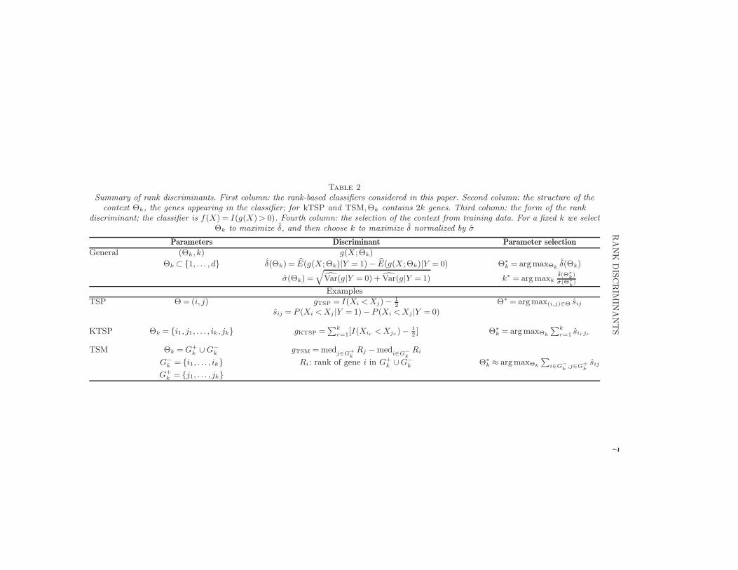
Table 2

Summary of rank discriminants. First column: the rank-based classifiers considered in this paper. Second column: the structure of thecontext Θk, the genes appearing in the classifier; for kTSP and TSM,Θk contains 2k genes. Third column: the form of the rank

discriminant; the classifier is f(X) = I(g(X)> 0). Fourth column: the selection of the context from training data. For a fixed k we selectΘk to maximize δ, and then choose k to maximize δ normalized by σ

Parameters Discriminant Parameter selection

General (Θk, k) g(X;Θk)

Θk ⊂ 1, . . . , d δ(Θk) = E(g(X;Θk)|Y = 1)− E(g(X;Θk)|Y = 0) Θ∗k = argmaxΘk

δ(Θk)

σ(Θk) =

√Var(g|Y = 0) + Var(g|Y = 1) k∗ = argmaxk

δ(Θ∗

k)

σ(Θ∗

k)

Examples

TSP Θ= (i, j) gTSP = I(Xi <Xj)−12

Θ∗ = argmax(i,j)∈Θ sijsij = P (Xi <Xj |Y = 1)− P (Xi <Xj |Y = 0)

KTSP Θk = i1, j1, . . . , ik, jk gKTSP =∑k

r=1[I(Xir <Xjr )−12] Θ∗

k = argmaxΘk

∑k

r=1 sirjr

TSM Θk =G+k ∪G−

k gTSM =medj∈G

+

k

Rj −medi∈G

−

k

Ri

G−k = i1, . . . , ik Ri: rank of gene i in G+

k ∪G−k Θ∗

k ≈ argmaxΘk

∑i∈G

−

k,j∈G

+

k

sij

G+k = j1, . . . , jk


equally-sized sets of genes and the average ranks were compared. Since thedirect extension of TSP score maximization was computationally impossi-ble, and likely to badly overfit the data, the sets were selected by splittingtop-scoring pairs and repeated random sampling. Although ad hoc, thisprocess further demonstrated the discriminating power of rank statistics formicroarray data.

Finally, there is some related work about ratios of concentrations (whichare natural in chemical terms) for diagnosis and prognosis. That work isnot rank-based but retains invariance to scaling. Golub et al. (1999) dis-tinguished between malignant pleural mesothelioma (MPM) and adenocar-cinoma (ADCA) of the lung by combining multiple ratios into a single di-agnostic tool, and Ma et al. (2004) found that a two-gene expression ratioderived from a genome-wide, oligonucleotide microarray analysis of estrogenreceptor (ER)-positive, invasive breast cancers predicts tumor relapse andsurvival in patients treated with tamoxifen, which is crucial for early-stagebreast cancer management.

3. Rank-in-context classification. In this section we introduce a generalframework for rank-based classifiers using comparisons among a limitednumber of gene expressions, called the context. In addition, we describea general method to select the context, which is inspired by the analysisof variance paradigm of classical statistics. These classifiers have the RICproperty that they depend on the sample training data solely through thecontext selection; in other words, given the context, the classifiers have afixed decision boundary and do not depend on any further learning from thetraining data. For example, as will be seen in later sections, the Top-ScoringPair (TSP) classifier is RIC. Once a pair of genes (i.e., the context) is spec-ified, the TSP decision boundary is fixed and corresponds to a 45-degreeline going through the origin in the feature space defined by the two genes.This property confers to RIC classifiers a minimal-training property, whichmakes them insensitive to small disturbances to the ranks of the trainingdata, reducing variance and overfitting, and rendering them especially suit-able to the n≪ d settings illustrated in Table 1. We will demonstrate thegeneral RIC framework with two specific examples, namely, the previouslyintroduced KTSP classifier based on majority voting among comparisons[Tan et al. (2005)], as well as a new classifier based on the comparison ofthe medians, the Top-Scoring Medians (TSM ) classifier.

3.1. RIC discriminant. Let X= (X1,X2, . . . ,Xd) denote the expressionvalues of d genes on an expression microarray. Our objective is to use X todistinguish between two conditions or phenotypes for the cells in the assayedtissue, denoted Y = 0 and Y = 1. A classifier f associates a label f(X) ∈


0,1 with a given expression vector X. Practical classifiers are inferred fromtraining data, consisting of i.i.d. pairs Sn = (X(1), Y (1)), . . . , (X(n), Y (n)).

The classifiers we consider in this paper are all defined in terms of a generalrank-in-context discriminant g(X;Θ(Sn)), which is defined as a real-valuedfunction on the ranks of X over a subset of genes Θ(Sn)⊂ 1, . . . , d, which isdetermined by the training data Sn and is called the context of the classifier(the order of indices in the context may matter). The corresponding RIC

classifier f is defined by

f(X;Θ(Sn)) = I(g(X;Θ(Sn))> t) =

1, g(X;Θ(Sn))> t,

0, otherwise,(1)

where I(E) denotes the indicator variable of event E. The threshold pa-rameter t can be adjusted to achieve a desired specificity and sensitivity(see Section 3.4 below); otherwise, one usually sets t= 0. For simplicity wewill write Θ instead of Θ(Sn), with the implicit understanding that in RICclassification Θ is selected from the training data Sn.

We will consider two families of RIC classifiers. The first example is the k-Top Scoring Pairs (KTSP) classifier, which is a majority-voting rule amongk pairs of genes [Tan et al. (2005)]; KTSP was the winning entry of theInternational Conference in Machine Learning and Applications (ICMLA)2008 challenge for micro-array classification [Geman et al. (2008)]. Here,the context is partitioned into a set of gene pairs Θ = (i1, j1), . . . , (ik, jk),where k is a positive odd integer, in such a way that all pairs are disjoint,that is, all 2k genes are distinct. The RIC discriminant is given by

gKTSP(X; (i1, j1), . . . , (ik, jk)) =

k∑

r=1

[I(Xir <Xjr)−

1

2

].(2)

This KTSP RIC discriminant simply counts positive and negative “votes”in favor of ascending or descending ranks, respectively. The KTSP classifieris given by (1), with t= 0, which yields

fKTSP(X; (i1, j1), . . . , (ik, jk)) = I

(k∑

r=1

I(Xir <Xjr)>k

2

).(3)

The KTSP classifier is thus a majority-voting rule: it assigns label 1 tothe expression profile if the number of ascending ranks exceeds the numberof descending ranks in the context. The choice of odd k avoids the pos-sibility of a tie in the vote. If k = 1, then the KTSP classifier reduces tofTSP(X; (i, j)) = I(Xi <Xj), the Top-Scoring Pair (TSP) classifier [Gemanet al. (2004)].

The second example of an RIC classifier we propose is the Top Scoring

Median (TSM ) classifier, which compares the median rank of two sets of


genes. The median rank has the advantage that for any individual samplethe median is the value of one of the genes. Hence, in this sense, a comparisonof medians for a given sample is equivalent to the comparison of two-geneexpressions, as in the TSP decision rule. Here, the context is partitionedinto two sets of genes, Θ = G+

k ,G−k , such that |G+

k | = |G−k | = k, where k

is again a positive odd integer, and G+k and G−

k are disjoint, that is, all 2kgenes are distinct. Let Ri be the rank of Xi in the context Θ =G+

k ∪G−k ,

such that Ri = j if Xi is the jth smallest value among the gene expressionvalues indexed by Θ. The RIC discriminant is given by

gTSM(X;G+k ,G

−k ) = med

j∈G+k

Rj − medi∈G−

k

Ri,(4)

where “med” denotes the median operator. The TSM classifier is then givenby (1), with t= 0, which yields

fTSM(X;G+k ,G

−k ) = I

(medj∈G+

k

Rj > medi∈G−

k

Ri

).(5)

Therefore, the TSM classifier outputs 1 if the median of ranks in G+k exceeds

the median of ranks in G−k , and 0 otherwise. Notice that this is equivalent

to comparing the medians of the raw expression values directly. We remarkthat an obvious variation would be to compare the average rank rather thanthe median rank, which corresponds to the “TSPG” approach defined inXu, Geman and Winslow (2007), except that in that study, the context forTSPG was selected by splitting a fixed number of TSPs. We observed thatthe performances of the mean-rank and median-rank classifiers are similar,with a slight superiority of the median-rank (data not shown).

3.2. Criterion for context selection. The performance of RIC classifierscritically depends on the appropriate choice of the context Θ ⊂ 1, . . . , d.We propose a simple yet powerful procedure to select Θ from the trainingdata Sn. To motivate the proposed criterion, first note that a necessarycondition for the context Θ to yield a good classifier is that the discriminantg(X;Θ) has sufficiently distinct distributions under Y = 1 and Y = 0. Thiscan be expressed by requiring that the difference between the expected valuesof g(X;Θ) between the populations, namely,

δ(Θ) =E[g(X;Θ)|Y = 1, Sn]−E[g(X;Θ)|Y = 0, Sn],(6)

be maximized. Notice that this maximization is with respect to Θ alone; g isfixed and chosen a priori. In practice, one employs the maximum-likelihoodempirical criterion

δ(Θ) = E[g(X;Θ)|Y = 1, Sn]− E[g(X;Θ)|Y = 0, Sn],(7)


where

E[g(X;Θ)|Y = c,Sn] =

∑ni=1 g(X

(i);Θ)I(Y (i) = c)∑ni=1 I(Y

(i) = c),(8)

for c= 0,1.In the case of KTSP, the criterion in (6) becomes

δKTSP((i1, j1), . . . , (ik, jk)) =

k∑

r=1

sirjr ,(9)

where the pairwise score sij for the pair of genes (i, j) is defined as

sij = P (Xi <Xj |Y = 1)−P (Xi <Xj |Y = 0).(10)

Notice that if the pair of random variables (Xi,Xj) has a continuous distri-bution, so that P (Xi =Xj) = 0, then sij = −sji. In this case Xi <Xj canbe replaced by Xi ≤Xj in sij in (10).

The empirical criterion δKTSP((i1, j1), . . . , (ik, jk)) [cf. equation (7)] is ob-tained by substituting in (9) the empirical pairwise scores

sij = P (Xi <Xj |Y = 1)− P (Xi <Xj |Y = 0).(11)

Here the empirical probabilities are defined by P (Xi <Xj|Y = c) = E[I(Xi <

Xj)|Y = c], for c= 0,1, where the operator E is defined in (8).For TSM, the criterion in (6) is given by

δTSM(G+k ,G

−k )

(12)

=E[medj∈G+

k

Rj − medi∈G−

k

Ri|Y = 1]−E

[medj∈G+

k

Rj − medi∈G−

k

Ri|Y = 0].

Proposition S1 in Supplement A [Afsari, Braga-Neto and Geman (2014a)]shows that, under some assumptions,

δTSM(G+k ,G

−k ) =

2

k

∑

i∈G−k,j∈G+

k

sij,(13)

where sij is defined in (10).The difference between the two criteria (9) for KTSP and (13) for TSM

for selecting the context is that the former involves scores for k expressioncomparisons and the latter involves k2 comparisons since each gene i ∈G−

kis paired with each gene j ∈G+

k . Moreover, using the estimated solution tomaximizing (9) (see below) to construct G−

k and G+k by putting the first

gene from each pair into one and the second gene from each pair into theother does not work as well in maximizing (13) as the algorithms describedbelow.


The distributional smoothness conditions Proposition S1 are justified if kis not too large (see Supplement A [Afsari, Braga-Neto and Geman (2014a)]).

Finally, the empirical criterion δTSM(G+k ,G

−k ) can be calculated by substi-

tuting in (13) the empirical pairwise scores sij defined in (11).

3.3. Maximization of the criterion. Maximization of (6) or (7) works wellas long as the size of the context |Θ|, that is, the number of context genes, iskept fixed, because the criterion tends to be monotonically increasing with|Θ|, which complicates selection. We address this problem by proposing amodified criterion, which is partly inspired by the principle of analysis ofvariance in classical statistics. This modified criterion penalizes the additionof more genes to the context by requiring that the variance of g(X;Θ) withinthe populations be minimized. The latter is given by

σ(Θ) =

√Var(g(X;Θ)|Y = 0, Sn) + Var(g(X;Θ)|Y = 1, Sn),(14)

where Var is the maximum-likelihood estimator of the variance,

Var(g(X;Θ)|Y = c,Sn)

=

∑ni=1(g(X

(i);Θ)− E[g(X;Θ)|Y = c,Sn])2I(Y (i) = c)∑n

i=1 I(Y(i) = c)

,

for c= 0,1. The modified criterion to be maximized is

τ(Θ) =δ(Θ)

σ(Θ).(15)

The statistic τ(Θ) resembles the Welch two-sample t-test statistic of classicalhypothesis testing [Casella and Berger (2002)].

Direct maximization of (7) or (15) is in general a hard computationalproblem for the numbers of genes typically encountered in expression data.We propose instead a greedy procedure. Assuming that a predefined rangeof values Ω for the context size |Θ| is given, the procedure is as follows:

(1) For each value of k ∈Ω, an optimal context Θ∗k is chosen that maxi-

mizes (7) among all contexts Θk containing k genes:

Θ∗k = arg max

|Θ|=kδ(Θ).

(2) An optimal value k∗ is chosen that maximizes (15) among all contextsΘ∗

k|k ∈Ω obtained in the previous step:

k∗ = argmaxk∈Ω

τ(Θ∗k).


For KTSP, the maximization in step (1) of the previous context selectionprocedure becomes

(i∗1, j∗1), . . . , (i

∗k, j

∗k)= arg max

(i1,j1),...,(ik,jk)δKTSP((i1, j1), . . . , (ik, jk))

(16)

= arg max(i1,j1),...,(ik,jk)

k∑

r=1

sirjr .

We propose a greedy approach to this maximization problem: initializethe list with the top-scoring pair of genes, then keep adding pairs to thelist whose genes have not appeared so far [ties are broken by the secondaryscore proposed in Xu et al. (2005)]. This process is repeated until k pairs arechosen and corresponds essentially to the same method that was proposed,for fixed k, in the original paper on KTSP [Tan et al. (2005)]. Thus, thepreviously proposed heuristic has a justification in terms of maximizing theseparation between the rank discriminant (2) across the classes.

To obtain the optimal value k∗, one applies step (2) of the context selectionprocedure, with a range of values k ∈ Ω = 3,5, . . . ,K, for odd K (k = 1can be added if 1-TSP is considered). Note that here

σKTSP(Θ)

(17)

=

√√√√Var

(k∑

r=1

[I(Xi∗r <Xj∗r )]

∣∣∣∣Y = 0

)+ Var

(k∑

r=1

[I(Xi∗r <Xj∗r )]

∣∣∣∣Y = 1

).

Therefore, the optimal value of k is selected by

k∗ = arg maxk=3,5,...,K

τKTSP((i∗1, j

∗1), . . . , (i

∗k, j

∗k)),(18)

where

τKTSP((i∗1, j

∗1), . . . , (i

∗k, j

∗k))

=δKTSP((i

∗1, j

∗1), . . . , (i

∗k, j

∗k))

σKTSP((i∗1, j∗1), . . . , (i

∗k, j

∗k))

(19)

=

∑kr=1 si∗rj∗r√

Var(∑k

r=1[I(Xi∗r <Xj∗r )]|Y = 0) + Var(∑k

r=1[I(Xi∗r <Xj∗r )]|Y = 1).

Finally, the optimal context is then given by Θ∗ = (i∗1, j∗1), . . . , (i

∗k∗ , j

∗k∗).

For TSM, the maximization in step (1) of the context selection procedurecan be written as

(G+,∗k ,G−,∗

k ) = arg max(G+

k,G−

k)δTSM(G+

k ,G−k ) = arg max

(G+k,G−

k)

∑

i∈G−k,j∈G+

k

sij.(20)


Finding the global maximum in (20) is not feasible in general. We considera suboptimal strategy for accomplishing this task: sequentially construct thecontext by adding two genes at a time. Start by selecting the TSP pair i, jand setting G−

1 = i and G+1 = j. Then select the pair of genes i′, j′

distinct from i, j such that the sum of scores is maximized by G−2 = i, i′

and G+2 = j, j′, that is, δTSM(G+

k ,G−k ) is maximized over all sets G+

k ,G−k

of size two, assuming i ∈G−k and j ∈G+

k . This involves computing three newscores. Proceed in this way until k pairs have been selected.

To obtain the optimal value k∗, one applies step (2) of the context selectionprocedure, with a range of values k ∈ Ω = 3,5, . . . ,K, for odd K (thechoice of Ω is dictated by the facts that k = 1 reduces to 1-TSP, whereasProposition S1 does not hold for even k):

k∗ = arg maxk=3,5,...,K

τTSM(G+,∗k ,G−,∗

k ),

where

τTSM(G+,∗k ,G−,∗

k )

=δTSM(G+,∗

k ,G−,∗k )

σTSM(G+,∗k ,G−,∗

k )

=(E[med

j∈G+,∗k

Rj − medi∈G−,∗

k

Ri|Y = 1]− E

[med

j∈G+,∗k


k

Ri|Y = 0])

(21)

/(Var(med

j∈G+,∗k


k

Ri|Y = 0)

+ Var(med

j∈G+,∗k


k

Ri|Y = 1))1/2

.

Notice that τTSM is defined directly by replacing (4) into (7) and (14), andthen using (15). In particular, it does not use the approximation in (13).Finally, the optimal context is given by Θ∗ = (G+,∗

k∗ ,G−,∗k∗ ).

For both KTSP and TSM classifiers, the step-wise process to performthe maximization of the criterion [cf. equations (16) and (20)] does not needto be restarted as k increases, since the suboptimal contexts are nested [bycontrast, the method in Tan et al. (2005) employed cross-validation to choosek∗]. The detailed context selection procedure for KTSP and TSM classifiersis given in Algorithms S1 and S2 in Supplement C [Afsari, Braga-Neto andGeman (2014c)].

3.4. Error rates. In this section we discuss the choice of the threshold tused in (1). The sensitivity is defined as P (f(X) = 1|Y = 1) and the speci-

ficity is defined as P (f(X) = 0|Y = 0). We are interested in controlling both,


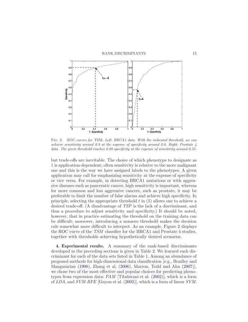
Fig. 2. ROC curves for TSM. Left: BRCA1 data. With the indicated threshold, we canachieve sensitivity around 0.9 at the expense of specificity around 0.6. Right: Prostate 4data. The given threshold reaches 0.88 specificity at the expense of sensitivity around 0.55.

but trade-offs are inevitable. The choice of which phenotype to designate as1 is application-dependent; often sensitivity is relative to the more malignantone and this is the way we have assigned labels to the phenotypes. A givenapplication may call for emphasizing sensitivity at the expense of specificityor vice versa. For example, in detecting BRCA1 mutations or with aggres-sive diseases such as pancreatic cancer, high sensitivity is important, whereasfor more common and less aggressive cancers, such as prostate, it may bepreferable to limit the number of false alarms and achieve high specificity. Inprinciple, selecting the appropriate threshold t in (1) allows one to achieve adesired trade-off. (A disadvantage of TSP is the lack of a discriminant, andthus a procedure to adjust sensitivity and specificity.) It should be noted,however, that in practice estimating the threshold on the training data canbe difficult; moreover, introducing a nonzero threshold makes the decisionrule somewhat more difficult to interpret. As an example, Figure 2 displaysthe ROC curve of the TSM classifier for the BRCA1 and Prostate 4 studies,together with thresholds achieving hypothetically desired scenarios.

4. Experimental results. A summary of the rank-based discriminantsdeveloped in the preceding sections is given in Table 2. We learned each dis-criminant for each of the data sets listed in Table 1. Among an abundance ofproposed methods for high-dimensional data classification [e.g., Bradley andMangasarian (1998), Zhang et al. (2006), Marron, Todd and Ahn (2007)],we chose two of the most effective and popular choices for predicting pheno-types from expression data: PAM [Tibshirani et al. (2002)], which is a formof LDA, and SVM-RFE [Guyon et al. (2002)], which is a form of linear SVM.


Generalization errors are estimated with cross-validation, specifically av-eraging the results of ten repetitions of 10-fold CV, as recommended inBraga-Neto and Dougherty (2004) and Hastie, Tibshirani and Friedman(2001). Despite the inaccuracy of small-sample cross-validation estimates[Braga-Neto and Dougherty (2004)], 10-fold CV suffices to obtain the broadperspective on relative performance across many different data sets.

The protocols for training (including parameter selection) are given below.To reduce computation, we filter the whole gene pool without using the classlabels before selecting the context for rank discriminants (TSP, KTSP andTSM ). Although a variety of filtering methods exist in the literature, such asPAM [Tibshirani et al. (2002)], SIS [Fan and Lv (2008)], Dantzig selector[Candes and Tao (2007)] and the Wilcoxon-rank test [Wilcoxon (1945)],we simply use an average signal filter: select the 4000 genes with highestmean rank (across both classes). In particular, there is no effort to detect“differentially expressed” genes. In this way we minimize the influence ofthe filtering method in assessing the performance of rank discriminants:

• TSP : The single pair maximizing sij over all pairs in the 4000 filteredgenes, breaking scoring ties if necessary with the secondary score proposedin Xu et al. (2005).

• KTSP : The k disjoint pairs maximizing sij over all pairs in the 4000filtered genes with the same tie-breaking method. The number of pairs kis determined via Algorithm S1, within the range k = 3,5, . . . ,9, avoidingties in voting. Notice that k = 1 is excluded so that KTSP cannot reduceto TSP. We tried also k = 3,5, . . . ,49 and the cross-validated accuracieschanged insignificantly.

• TSM : The context is chosen from the top 4000 genes by the greedy se-lection procedure described in Algorithm S2. The size of the two sets forcomputing the median rank is selected in the range k = 3,5,7,9 (provid-ing a unique median and thereby rendering Proposition S1 applicable).We also tried k = 3,5, . . . ,49 and again the changes in the cross-validatedaccuracies were insignificant.

• SVM-RFE : We learned two linear SVM s using SVM-RFE : one with tengenes and one with a hundred genes. No filtering was applied, since SVM-

RFE itself does that. Since we found that the choice of the slack variablebarely changes the results, we fix C = 0.1. (In fact, the data are linearlyseparable in nearly all loops.) Only the results for SVM-RFE with a hun-dred genes are shown since it was almost 3% better than with ten genes.

• PAM : We use the automatic filtering mechanism provided by Tibshirani(2011). The prior class likelihoods were set to 0.5 and all other param-eters were set to default values. The most important parameter is thethreshold; the automatic one chosen by the program results in relativelylower accuracy than the other methods (84.00%) on average. Fixing the


threshold and choosing the best one over all data sets only increases theaccuracy by one percent. Instead, for each data set and each threshold, weestimated the cross-validated accuracy for PAM and report the accuracyof the best threshold for that data set.

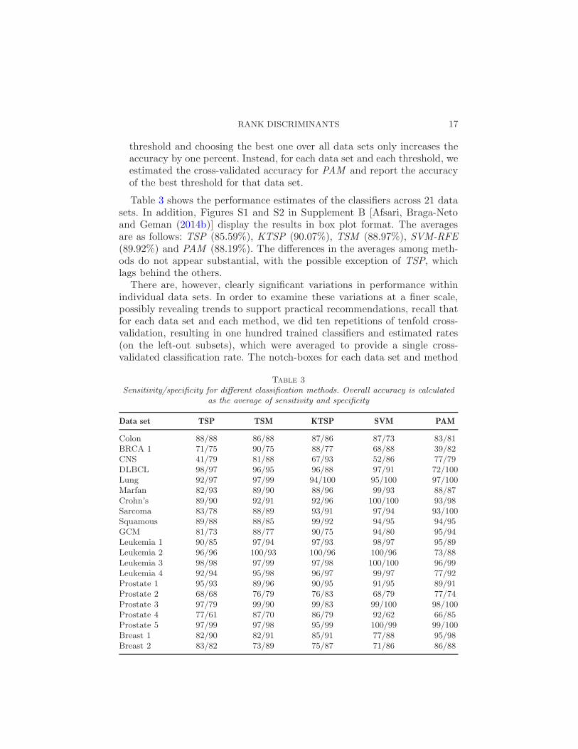
Table 3 shows the performance estimates of the classifiers across 21 datasets. In addition, Figures S1 and S2 in Supplement B [Afsari, Braga-Netoand Geman (2014b)] display the results in box plot format. The averagesare as follows: TSP (85.59%), KTSP (90.07%), TSM (88.97%), SVM-RFE

(89.92%) and PAM (88.19%). The differences in the averages among meth-ods do not appear substantial, with the possible exception of TSP, whichlags behind the others.

There are, however, clearly significant variations in performance withinindividual data sets. In order to examine these variations at a finer scale,possibly revealing trends to support practical recommendations, recall thatfor each data set and each method, we did ten repetitions of tenfold cross-validation, resulting in one hundred trained classifiers and estimated rates(on the left-out subsets), which were averaged to provide a single cross-validated classification rate. The notch-boxes for each data set and method

Table 3

Sensitivity/specificity for different classification methods. Overall accuracy is calculatedas the average of sensitivity and specificity

Data set TSP TSM KTSP SVM PAM

Colon 88/88 86/88 87/86 87/73 83/81BRCA 1 71/75 90/75 88/77 68/88 39/82CNS 41/79 81/88 67/93 52/86 77/79DLBCL 98/97 96/95 96/88 97/91 72/100Lung 92/97 97/99 94/100 95/100 97/100Marfan 82/93 89/90 88/96 99/93 88/87Crohn’s 89/90 92/91 92/96 100/100 93/98Sarcoma 83/78 88/89 93/91 97/94 93/100Squamous 89/88 88/85 99/92 94/95 94/95GCM 81/73 88/77 90/75 94/80 95/94Leukemia 1 90/85 97/94 97/93 98/97 95/89Leukemia 2 96/96 100/93 100/96 100/96 73/88Leukemia 3 98/98 97/99 97/98 100/100 96/99Leukemia 4 92/94 95/98 96/97 99/97 77/92Prostate 1 95/93 89/96 90/95 91/95 89/91Prostate 2 68/68 76/79 76/83 68/79 77/74Prostate 3 97/79 99/90 99/83 99/100 98/100Prostate 4 77/61 87/70 86/79 92/62 66/85Prostate 5 97/99 97/98 95/99 100/99 99/100Breast 1 82/90 82/91 85/91 77/88 95/98Breast 2 83/82 73/89 75/87 71/86 86/88


are plotted in Figures S1 and S2 (Supplement B [Afsari, Braga-Neto andGeman (2014b)]). As is commonly done, any two methods will be declaredto be “tied” on a given data set if the notches overlap; otherwise, that is, ifthe notches are disjoint, the “winner” is taken to be the one with the largermedian.

First, using the “notch test” to compare the three RIC classifiers, KTSP

slightly outperformsTSM, which in turn outperformsTSP. More specifically,KTSP has accuracy superior to both others on ten data sets. In terms ofKTSP vs TSM, KTSP outperforms on three data sets, vice versa on onedata set and they tie on all others. Moreover, TSM outperforms TSP onnine data sets and vice versa on two data sets. As a result, if accuracy is thedominant concern, we recommend KTSP among the RIC classifiers, whereasif simplicity, transparency and links to biological mechanisms are important,one might prefer TSP. Comparisons with non-RIC methods (see below) arebased on KTSP, although substituting TSM does not lead to appreciablydifferent conclusions.

Second, SVM performs better than PAM on six data sets and PAM onthree data sets. Hence, in the remainder of this section we will compareKTSP with SVM. We emphasize that the comparison between PAM andSVM is on our particular data sets, using our particular measures of per-formance, namely, cross-validation to estimate accuracy and the notch testfor pairwise comparisons. Results on other data sets or in other conditionsmay differ.

Third, whereas the overall performance statistics for KTSP and SVM arealmost identical, trends do emerge based on sample size, which is obviouslyan important parameter and especially useful here because it varies consid-erably among our data sets (Table 1). To avoid fine-tuning, we only considera coarse and somewhat arbitrary quantization into three categories: “small,”“medium” and “large” data sets, defined, respectively, by fewer than 100 (to-tal) samples (twelve data sets), 100–200 samples (five data sets) and morethan 200 samples (four data sets). On small data sets, KTSP outperformsSVM on four data sets and never vice versa; for medium data sets, eachoutperforms the other on one of the five data sets; and SVM outperformsKTSP on three out of four large data sets and never vice versa.

Another criterion is sparsity: the number of genes used by TSP is alwaystwo and by SVM-RFE is always one hundred. Averaged across all data setsand loops of cross-validation, KTSP uses 12.5 genes, TSM uses 10.16 genes,and PAM uses 5771 genes.

Finally, we performed an experiment to roughly gauge the variability inselecting the genes in the support of the various classifiers. Taking advantageof the fact that we train 100 different classifiers for each method and dataset, each time with approximately the same number of examples, we define a“consistency” measure for a pair of classifiers as the average support overlap


over all distinct pairs of runs. That is, for any given data set and method,and any two loops of cross-validation, let S1 and S2 be the supports (set

of selected genes) and define the overlap as |S1∩S2||S1∪S2|

. This fraction is then

averaged over all 100(99)/2 pairs of loops, and obviously ranges from zero(no consistency) to one (consistency in all loops). Whereas in 16 of the21 data sets KTSP had a higher consistency score than SVM, the moreimportant point is that in both cases the scores are low in absolute terms,which coheres with other observations about the enormous variations inlearned genes signatures.

5. Discussion and conclusions. What might be a “mechanistic interpre-tation” of the TSP classifier, where the context consists of only two genes?In Price et al. (2007), a reversal between the two genes Prune2 and Obscurinis shown to be an accurate test for separating GIST and LMS. Providing anexplanation, a hypothesized mechanism, is not straightforward, although ithas been recently shown that both modulate RhoA activity (which controlsmany signaling events): a splice variant of Prune2 is reported to decreaseRhoA activity when over-expressed and Obscurin contains a Rho-GEF bind-ing domain which helps to activate RhoA [Funk (2012)].

Generically, one of the most elementary regulatory motifs is simply Ainhibits B (denoted A ⊣B). For example, A may be constitutively “on” andB constitutively “off” after development. Perhaps A is a transcription factoror involved in methylation of B. In the normal phenotype we see A expressed,but perhaps A becomes inactivated in the cancer phenotype, resulting in theexpression of B, and hence an expression reversal from normal to cancer. Stillmore generally, a variety of regulatory feedback loops have been identifiedin mammals. For instance, an example of a bi-stable loop is shown below.

Due to the activation and suppression patterns depicted in Figure 3, wemight expect P (XA1 < XA2 |Y = 0) ≫ P (XA1 < XA2 |Y = 1) and P (XB1 <XB2 |Y = 0)≪ P (XB1 <XB2 |Y = 1). Thus, there are two expression rever-sals, one between the two miRNAs and one, in the opposite direction, be-tween the two mRNAs. Given both miRNA and mRNA data, we mightthen build a classifier based on these two switches. For example, the rank

Fig. 3. A bi-stable feedback loop. Molecules A1, A2 (resp., B1, B2) are from the samespecies, for example, two miRNAs (resp., two mRNAs). Letters in boldface indicate an“on” state.


discriminant might simply be 2-TSP, the number of reversals observed. Ac-cordingly, we have argued that expression comparisons may provide an ele-mentary building block for a connection between rank-based decision rulesand potential mechanisms.

We have reported extensive experiments with classifiers based on expres-sion comparisons with different diseases and microarray platforms and com-pared the results with other methods which usually use significantly moregenes. No one classifier, whether within the rank-based collection or betweenthem and other methods such as SVM and PAM, uniformly dominates. Themost appropriate one to use is likely to be problem-dependent. Moreover,until much larger data sets become available, it will be difficult to obtainhighly accurate estimates of generalization errors. What does seem apparentis that our results support the conclusions reached in earlier studies [Dudoit,Fridlyand and Speed (2002), Braga-Neto (2007), Wang (2012), Simon et al.(2003)] that simple classifiers are usually competitive with more complexones with microarray data and limited samples. This has important conse-quences for future developments in functional genomics since one key thrustof “personalized medicine” is an attempt to learn appropriate treatments fordisease subtypes, which means sample sizes will not necessarily get largerand might even get smaller. Moreover, as attention turns increasingly towardtreatment, potentially mechanistic characterizations of statistical decisionswill become of paramount importance for translational medicine.

SUPPLEMENTARY MATERIAL

Proposition S1 (DOI: 10.1214/14-AOAS738SUPPA; .pdf). We providethe statement and proof of Proposition S1 as well as statistical tests for theassumptions made in Proposition S1.

Notch-plots for classification accuracies (DOI: 10.1214/14-AOAS738SUPPB;.pdf). We provide notch-plots of the estimates of classification accuracyfor every method and every data set based on ten runs of tenfold cross-validation.

Algorithms for KTSP and TSM (DOI: 10.1214/14-AOAS738SUPPC; .pdf).We provide a summary of the algorithms for learning the KTSP and TSMclassifiers.

REFERENCES

Afsari, B., Braga-Neto, U. M. and Geman, D. (2014a). Supplementto “Rank discriminants for predicting phenotypes from RNA expression.”DOI:10.1214/14-AOAS738SUPPA.

Afsari, B., Braga-Neto, U. M. and Geman, D. (2014b). Supplementto “Rank discriminants for predicting phenotypes from RNA expression.”DOI:10.1214/14-AOAS738SUPPB.

http://dx.doi.org/10.1214/14-AOAS738SUPPA

http://dx.doi.org/10.1214/14-AOAS738SUPPB

http://dx.doi.org/10.1214/14-AOAS738SUPPC

http://dx.doi.org/10.1214/14-AOAS738SUPPA

http://dx.doi.org/10.1214/14-AOAS738SUPPB


Afsari, B., Braga-Neto, U. M. and Geman, D. (2014c). Supplementto “Rank discriminants for predicting phenotypes from RNA expression.”DOI:10.1214/14-AOAS738SUPPC.

Alon, U., Barkai, N., Notterman, D. et al. (1999). Broad patterns of gene expressionrevealed by clustering analysis of tumor and normal colon tissues probed by oligonu-cleotide arrays. Proc. Natl. Acad. Sci. USA 96 6745–6750.

Altman, R. B., Kroemer, H. K., McCarty, C. A. (2011). Pharmacogenomics: Willthe promise be fulfilled. Nat. Rev. 12 69–73.

Anderson, T., Tchernyshyov, I., Diez, R. et al. (2007). Discovering robust proteinbiomarkers for disease from relative expression reversals in 2-D DIGE data. Proteomics7 1197–1208.

Armstrong, S. A., Staunton, J. E., Silverman, L. B. et al. (2002). MLL translocationsspecify a distinct gene expression profile that distinguishes a unique leukemia. Nat.Genet. 30 41–47.

Auffray, C. (2007). Protein subnetwork markers improve prediction of cancer outcome.Mol. Syst. Biol. 3 1–2.

Bicciato, S., Pandin, M., Didone, G. and Bello, C. D. (2003). Pattern identifica-tion and classification in gene expression data using an autoassociative neural networkmodel. Biotechnol. Bioeng. 81 594–606.

Bloated, B., Irizarry, R. and Speed, T. (2004). A comparison of normalization meth-ods for high density oligonucleotide array data based on variance and bias. Bioinfor-matics 19 185–193.

Bloom, G., Yang, I., Boulware, D. et al. (2004). Multi-platform, multisite, microarray-based human tumor classification. Am. J. Pathol. 164 9–16.

Boulesteix, A. L., Tutz, George. and Strimmer, K. (2003). A CART-based approachto discover emerging patterns in microarray data. Bioinformatics 19 2465–2472.

Bradley, P. S. and Mangasarian, O. L. (1998). Feature selection via voncave mini-mization and support vector machines. In ICML 82–90. Morgan Kaufmann, Madison,WI.

Braga-Neto, U. M. (2007). Fads and fallacies in the name of small-sample microarrayclassification—a highlight of misunderstanding and erroneous usage in the applicationsof genomic signal processing. IEEE Signal Process. Mag. 24 91–99.

Braga-Neto, U. M. and Dougherty, E. R. (2004). Is cross-validation valid for small-sample microarray classification? Bioinformatics 20 374–380.

Buffa, F., Camps, C.,Winchester, L., Snell, C.,Gee, H., Sheldon, H., Taylor, M.,Harris, A. and Ragoussis, J. (2011). microRNA-associated progression pathways andpotential therapeutic targets identified by integrated mRNA and microRNA expressionprofiling in breast cancer. Cancer Res. 71 5635–5645.

Burczynski, M., Peterson, R., Twine, N. et al. (2006). Molecular classification ofCrohn’s disease and ulcerative colitis patients using transcriptional profiles in peripheralblood mononuclear cells. Cancer Res. 8 51–61.

Candes, E. and Tao, T. (2007). The Dantzig selector: Statistical estimation when p ismuch larger than n. Ann. Statist. 35 2313–2351. MR2382644

Casella, G. and Berger, R. L. (2002). Statistical Inference, 2nd ed. Duxbury, PacificGrove, CA.

Dettling, M. and Buhlmann, P. (2003). Boosting for tumor classification with geneexpression data. Bioinformatics 19 1061–1069.

Dudoit, S., Fridlyand, J. and Speed, T. P. (2002). Comparison of discriminationmethods for the classification of tumors using gene expression data. J. Amer. Statist.Assoc. 97 77–87. MR1963389

http://dx.doi.org/10.1214/14-AOAS738SUPPC

http://www.ams.org/mathscinet-getitem?mr=2382644



Edelman, L., Toia, G., Geman, D. et al. (2009). Two-transcript gene expression classi-fiers in the diagnosis and prognosis of human diseases. BMC Genomics 10 583.

Enerly, E., Steinfeld, I., Kleivi, K., Leivonen, S.-K. et al. (2011). miRNA–mRNAintegrated analysis reveals roles for miRNAs in primary breast tumors. PLoS ONE 60016915.

Evans, J. P., Meslin, E. M., Marteau, T. M. and Caulfield, T. (2011). Deflatingthe genomic bubble. Science 331 861–862.

Fan, J. and Fan, Y. (2008). High-dimensional classification using features annealed in-dependence rules. Ann. Statist. 36 2605–2637. MR2485009

Fan, J. and Lv, J. (2008). Sure independence screening for ultrahigh dimensional featurespace. J. R. Stat. Soc. Ser. B Stat. Methodol. 70 849–911. MR2530322

Funk, C. (2012). Personal communication. Institute for Systems Biology, Seattle, WA.Geman, D., d’Avignon, C., Naiman, D. Q. and Winslow, R. L. (2004). Classifying

gene expression profiles from pairwise mRNA comparisons. Stat. Appl. Genet. Mol.Biol. 3 Art. 19, 21 pp. (electronic). MR2101468

Geman, D., Afsari, B., Tan, A. C. and Naiman, D. Q. (2008). Microarray classificationfrom several two-gene expression comparisons. In Machine Learning and Applications,2008. ICMLA’08. Seventh International Conference 583–585. IEEE, San Diego, CA.

Golub, T. R., Slonim, D. K., Tamayo, P. et al. (1999). Molecular classification ofcancer: Class discovery and class prediction by gene expression monitoring. Science 286531–537.

Gordon, G. J., Jensen, R. V., Hsiao, L.-L., Gullans, S. R., Blumenstock, J. E.,Ramaswamy, S., Richards, W. G., Sugarbaker, D. J. and Bueno, R. (2002).Translation of microarray data into clinically relevant cancer diagnostic tests usinggene expression ratios in lung cancer and mesothelioma. Cancer Res. 62 4963–4967.

Guo, Y., Hastie, T. and Tibshirani, R. (2005). Regularized discriminant analysis andits application in microarrays. Biostatistics 1 1–18.

Guo, Y., Hastie, T. and Tibshirani, R. (2007). Regularized linear discriminant analysisand its application in microarrays. Biostatistics 8 86–100.

Guyon, I., Weston, J., Barnhill, S. and Vapnik, V. (2002). Gene selection for cancerclassification using support vector machines. Mach. Learn. 46 389–422.

Hastie, T., Tibshirani, R. and Friedman, J. (2001). The Elements of Statistical Learn-ing: Data Mining, Inference, and Prediction. Springer Series in Statistics. Springer, NewYork. MR1851606

Jones, S., Zhang, X., Parsons, D. W. et al. (2008). Core signaling pathways in humanpancreatic cancers revealed by global genomic analyses. Science 321 1801–1806.

Khan, J., Wei, J. S., Ringner, M. et al. (2001). Classification and diagnostic predictionof cancers using gene expression profiling and artificial neural networks. Nat. Med. 7673–679.

Kohlmann, A., Kipps, T. J., Rassenti, L. Z. and Downing, J. R. (2008). An inter-national standardization programme towards the application of gene expression pro-filing in routine leukaemia diagnostics: The microarray innovations in leukemia studyprephase. Br. J. Haematol. 142 802–807.

Kuriakose, M. A., Chen, W. T. et al. (2004). Selection and validation of differentiallyexpressed genes in head and neck cancer. Cell. Mol. Life Sci. 61 1372–1383.

Lee, E., Chuang, H. Y., Kim, J. W. et al. (2008). Inferring pathway activity towardprecise disease classification. PLoS Comput. Biol. 4 e1000217.

Lin, X., Afsari, B., Marchionni, L. et al. (2009). The ordering of expression among afew genes can provide simple cancer biomarkers and signal BRCA1 mutations. BMCBioinformatics 10 256.






Ma, X. J., Wang, Z., Ryan, P. D. et al. (2004). A two-gene expression ratio predictsclinical outcome in breast cancer patients treated with tamoxifen. Cancer Cell 5 607–616.

Marron, J. S., Todd, M. J. and Ahn, J. (2007). Distance-weighted discrimination. J.Amer. Statist. Assoc. 102 1267–1271. MR2412548

Marshall, E. (2011). Waiting for the revolution. Science 331 526–529.Mills, K. I., Kohlmann, A., Williams, P. M., Wieczorek, L. et al. (2009).

Microarray-based classifiers and prognosis models identify subgroups with distinct clin-ical outcomes and high risk of AML transformation of myelodysplastic syndrome. Blood114 1063–1072.

Peng, S., Xu, Q., Ling, X. et al. (2003). Molecular classification of cancer types from mi-croarray data using the combination of genetic algorithms and support vector machines.FEBS Lett. 555 358–362.

Pomeroy, C., Tamayo, P., Gaasenbeek, M. et al. (2002). Prediction of central nervoussystem embryonal tumour outcome based on gene expression. Nature 415 436–442.

Price, N., Trent, J., El-Naggar, A. et al. (2007). Highly accurate two-gene classi-fier for differentiating gastrointestinal stromal tumors and leimyosarcomas. Proc. Natl.Acad. Sci. USA 43 3414–3419.

Qu, Y., Adam, B., Yasui, Y. et al. (2002). Boosted decision tree analysis ofsurface-enhanced laser desorption/ionization mass spectral serum profiles discriminatesprostate cancer from noncancer patients. Clin. Chem. 48 1835–1843.

Ramaswamy, S., Tamayo, P., Rifkin, R. et al. (2001). Multiclass cancer diagnosis usingtumor gene expression signatures. Proc. Natl. Acad. Sci. USA 98 15149–15154.

Raponi, M., Lancet, J. E., Fan, H. et al. (2008). A 2-gene classifier for predictingresponse to the farnesyltransferase inhibitor tipifarnib in acute myeloid leukemia. Blood111 2589–2596.

Shipp, M., Ross, K., Tamayo, P. et al. (2002). Diffuse large B-cell lymphoma outcomeprediction by gene-expression profiling and supervised machine learning. Nat. Med. 868–74.

Simon, R., Radmacher, M. D., Dobbin, K. and McShane, L. M. (2003). Pitfalls inthe use of DNA microarray data for diagnostic and prognostic classification. J. Natl.Cancer Inst. 95 14–18.

Singh, D., Febbo, P., Ross, K. et al. (2002). Gene expression correlates of clinicalprostate cancer behavior. Cancer Cell 1 203–209.

Stuart, R., Wachsman, W., Berry, C. et al. (2004). In silico dissection of cell-type-associated patterns of gene expression in prostate cancer. Proc. Natl. Acad. Sci. USA101 615–620.

Tan, A. C., Naiman, D. Q., Xu, L. et al. (2005). Simple decision rules for classifyinghuman cancers from gene expression profiles. Bioinformatics 21 3896–3904.

Thomas, R. K., Baker, A. C., DeBiasi, R. M. et al. (2007). High-throughput oncogenemutation profiling in human cancer. Nature Genetics 39 347–351.

Tibshirani, R. (2011). PAM R Package. Available at http://www-stat.stanford.edu/

~tibs/PAM/Rdist/index.html.Tibshirani, R., Hastie, T., Narasimhan, B. and Chu, G. (2002). Diagnosis of multiple

cancer types by shrunken centroids of gene expression. Proc. Natl. Acad. Sci. USA 996567–6572.

Wang, X. (2012). Robust two-gene classifiers for cancer prediction. Genomics 99 90–95.Weichselbaum, R. R., Ishwaranc, H., Yoona, T. et al. (2008). An interferon-related

gene signature for DNA damage resistance is a predictive marker for chemotherapy andradiation for breast cancer. Proc. Natl. Acad. Sci. USA 105 18490–18495.


http://www-stat.stanford.edu/~tibs/PAM/Rdist/index.html

http://www-stat.stanford.edu/~tibs/PAM/Rdist/index.html


Welsh, J., Sapinoso, L., Su, A. et al. (2001). Analysis of gene expression identifiescandidate markers and pharmacological targets inprostate cancer. Cancer Res. 61 5974–5978.

Wilcoxon, F. (1945). Individual comparisons by ranking methods. Biometrics 80–83.Winslow, R., Trayanova, N., Geman, D. and Miller, M. (2012). The emerging dis-

cipline of computational medicine. Sci. Transl. Med. 4 158rv11.Xu, L., Geman, D. and Winslow, R. L. (2007). Large-scale integration of cancer mi-

croarray data identifies a robust common cancer signature. BMC Bioinformatics 8 275.Xu, L., Tan, A. C., Naiman, D. Q. et al. (2005). Robust prostate cancer marker genes

emerge from direct integration of inter-study microarray data. BMC Bioinformatics 213905–3911.

Yao, Z., Jaeger, J., Ruzzo, W. L. et al. (2004). Gene expression alterations in prostatecancer predicting tumor aggression and preceding development of malignancy. J. Cli.Oncol. 22 2790–2799.

Yao, Z., Jaeger, J., Ruzzo, W. et al. (2007). A Marfan syndrome gene expressionphenotype in cultured skin fibroblasts. BMC Genomics 8 319.

Yeang, C., Ramaswamy, S., Tamayo, P. et al. (2001). Molecular classification of mul-tiple tumor types. Bioinformatics 17 S316–S322.

Zhang, H., Yu, C. Y. and Singer, B. (2003). Cell and tumor classification using. Proc.Natl. Acad. Sci. USA 100 4168–4172.

Zhang, H. H., Ahn, J., Lin, X. and Park, C. (2006). Gene selection using supportvector machines with nonconvex penalty. Bioinformatics 22 88–95.

Zhao, H., Logothetis, C. J. and Gorlov, I. P. (2010). Usefulness of the top-scoringpairs of genes for prediction of prostate cancer progression. Prostate Cancer ProstaticDis. 13 252–259.

B. Afsari

Department of Electrical

and Computer Engineering

Johns Hopkins University

Baltimore, Maryland 21218

USA

E-mail: [email protected]

U. M. Braga-Neto

Department of Electrical

and Computer Engineering

Texas A&M University

College Station, Texas 77843

USA


D. Geman

Department of Applied Mathematics and Statistics

Johns Hopkins University

Baltimore, Maryland 21218

USA


mailto:[email protected]



rank discriminants for predicting phenotypes from rna ... file2 b. afsari, u. m. braga-neto and d....

Documents