Rapid biodiversity assessment of a Neotropical rainforest using soundscape recordings

Caspar Ström Student

Degree Thesis in Ecology 30 ECTS Master’s Level

Report passed: 14 June 2013 Supervisors: Folmer Bokma Jerome Sueur

Abstract Developing cheap and efficient methods to estimate biodiversity is an important task for

biodiversity conservation, especially in tropical forests where biodiversity inventories are

often difficult and expensive. Recently, a method was proposed to estimate biodiversity from

sound recordings, without species identification. I applied this method to soundscape

recordings from a tropical wet forest in Tortuguero, Costa Rica, to test its feasibility and cost-

effectiveness as a biodiversity indicator. I recorded in four rainforest sites that had been

subjected to varying degrees of logging in the past and that were therefore expected to differ

in their biodiversity. Several diversity indices were calculated using acoustic measures, which

were then compared between sites. Two new acoustic diversity indices, Hfp and βsor,

indicated differences between sites that were consistent with expectations based on logging

history. The method was demonstrated to be highly applicable in tropical wet forest and cost-

effective when compared with traditional taxonomic surveys. The study showed that methods

to estimate biodiversity from soundscape recordings have great potential for future use in

tropical conservation management.

Contents 1 Introduction ...........................................................................................................................1

2 Materials and Methods ........................................................................................................ 3

2.1 Study area ..................................................................................................................... 3

2.2 Recording sites ............................................................................................................. 3

2.2.1 Site TNP .................................................................................................................. 5

2.2.2 Site CT ................................................................................................................... 5

2.2.3 Site CPBS ............................................................................................................... 5

2.2.4 Site MS .................................................................................................................. 6

2.3 Methods ........................................................................................................................ 6

2.3.1 Spatial sampling .................................................................................................... 6

2.3.2 Time sampling ....................................................................................................... 6

2.3.3 Recording methods ............................................................................................... 9

2.3.4 Soundscape analyses ........................................................................................... 10

2.3.5 Statistical analyses .............................................................................................. 12

3 Results ................................................................................................................................ 12

3.1 Spatial heterogeneity .................................................................................................. 12

3.2 Time heterogeneity ..................................................................................................... 12

3.3 Frequency components .............................................................................................. 13

3.4 Weather ...................................................................................................................... 13

4 Discussion ........................................................................................................................... 17

4.1 Acoustic indices ........................................................................................................... 17

4.2 Spatio-temporal heterogeneity .................................................................................. 18

4.3 Cost-effectiveness ....................................................................................................... 19

4.4 Implications for conservation management of the Tortuguero area ........................ 19

4.5 Conclusions ................................................................................................................. 20

5 Acknowledgements ............................................................................................................ 21

6 References .......................................................................................................................... 21

1

1 Introduction With habitat destruction threatening biodiversity in many of the world’s biodiversity hotspots

and with limited time and resources for biodiversity conservation, it has become necessary to

find places to which conservation resources should be concentrated (Brooks et al. 2002,

Myers et al. 2000, Putz et al. 2001). In order to establish conservation priority, diversity

indices are commonly used to assess the condition of ecosystems. Two of the most widely

used diversity indices in ecology are the Shannon and Simpson indices, which measure

species diversity (Ricotta 2004). Species diversity has two main components: the number of

species (species richness) and the evenness of their relative abundances (Peet 1974, Smith &

Wilson 1996, Tuomisto 2012). Although there is general agreement that species diversity

indices are useful in ecology, they are still controversial because of uncertainty as to what

ecological phenomena they actually measure, and whether they are relevant for conservation

(Ricotta 2004, Tuomisto 2012). Some authors have suggested that indices of phylogenetic or

functional diversity are more relevant for conservation (review in Ricotta 2004).

Diversity indices have traditionally relied on species inventories, but in highly diverse

environments such as tropical rainforest inventories are expensive and time demanding

(Lawton et al. 1998). Recently the use of proxies or indicators of biodiversity has been

attempted as an alternative that can reduce the need for exhaustive species inventories in

tropical forests. For example, indicator taxa may be used to assess habitat intactness, or to

predict the occurrence of endemics (Brown 1997, Barlow et al. 2007). Successful use of

indicator taxa, however, requires good knowledge about distributions and taxon

complementarity, which is often lacking in the tropics (Moritz et al. 2001). Attempts to

identify indicator taxa which can predict species diversity has produced varying results in

tropical forests (Lawton et al. 1998, Barlow et al. 2007). Habitat mapping, using remote

sensing data, soil type or other environmental parameters, may also identify tropical forests

with high diversity of certain taxa (Peay et al. 2010, Pekin et al. 2012).

Recently, another proxy has received increasing interest: Sound recording technology

potentially presents a cheap and effective means to study biodiversity (Frommolt et al. 2008,

Snaddon et al. 2013). Sound recordings eliminate many of the costly and invasive aspects of

traditional inventories, and allow surveys to be done by non-experts (Penman et al. 2005,

Frommolt et al. 2008). By using automated recorders a single surveyor can record at multiple

locations simultaneously, reducing the number of field personnel needed (Penman et al.

2005). The calls of many animal species can be identified from sound recordings, using

automatic signal recognition, manual identification by trained experts upon playback or

human-in-the-loop-analysis (Wimmer et al. 2013). Automatic recognition algorithms have

been developed for bats, birds, amphibians, marine mammals, and insects, with recognition

rates up to 90%, but are not yet sufficiently advanced to deal with complex acoustic

environments with many overlapping signals from widely different species (Obrist et al.

2010).

Sound has two important properties that can be measured: amplitude and frequency.

Amplitude measures the magnitude of changes in atmospheric pressure caused by sound

waves, and is usually measured using the Root Mean Square or RMS, which is the square root

of the average squared amplitude of a signal. The form of the variation in amplitude over

time is called the amplitude envelope. Frequency is the number of changes in atmospheric

pressure per second. The human ear can discern sound frequencies between 20 Hz – 20 kHz,

2

frequencies above this range are termed ultrasound. Many animals can hear and produce

sounds far into the ultrasound spectrum. Of course, even though these sounds are inaudible

to humans they can be registered by microphones and recorded.

Sounds produced by animals are usually studied at the individual or species level. However,

animal sound production can also be viewed at a larger scale, i.e. at a community or

landscape scale. All sounds produced in a landscape constitute the so-called soundscape

(Schäfer 1977). The soundscape has been divided in biological, geophysical and

anthropogenic components, termed biophony, geophony and anthrophony, respectively

(Krause 1998, 2002). Diverse animal communities are often loud and appear unstructured;

this “cacophony” has been considered as a constraint by biologists trying to study specific

animal signals, but can contain useful information in itself (Krause 1987). According to the

Acoustic Niche Hypothesis sound can become a limited resource because of interference

among signals. The acoustic space is then partitioned into acoustic niches, defined by

different frequency ranges or time patterns (Krause 1987). Acoustic partitioning has been

observed for birds (Ficken et al. 1974), anurans (Gerhardt 1994), cicadas (Sueur 2002) and

orthopterans (Riede 1993).

The Acoustic Niche Hypothesis has important implications for conservation. In old,

undisturbed habitats animal signals have had more time to adapt to minimise interference

with each other, therefore the extent of acoustic partitioning should be a result of

evolutionary time and the degree of disturbance (Gage et al. 2001 and Krause 2002 via

Pijanowski et al. 2011). Also, higher species diversity should cause more acoustic niches to be

occupied when acoustic partitioning is effective. These assumptions enable simple acoustic

measures to be used to calculate “acoustic diversity indices”, which opens up possibilities for

quick and cost-effective methods for environmental monitoring and biodiversity assessment

(Riede 1993, Sueur et al. 2008 A).

Sueur et al. (2008) first developed an acoustic diversity index to assess the overall acoustic

complexity of the biophony. They made an index based on the Shannon index, which they

dubbed the Acoustic Entropy Index (H). It measures the heterogeneity across the frequency

spectrum and the amplitude envelope. The H index was successfully correlated with species

diversity in simulations. Modifications of this index have since been published (Villanueva-

Rivera et al. 2011, Depraetere et al. 2012). Acoustic indices to measure beta diversity,

phylogenetic and functional diversities have also been developed (Sueur et al. 2008 A, Gasc

et al. 2013).

Acoustic diversity indices can potentially be an important tool for conservation management

in areas with high diversity of vocalising animals, where resources for traditional biodiversity

surveys are limited and where species inventories are otherwise impractical. However, the

indices published so far need to be tested in different habitats before they can be applied in a

real conservation context. New indices also need to be constructed to measure acoustic

partitioning on different spatial and temporal scales. Furthermore, the feasibility and cost-

effectiveness of recording soundscapes for the purpose of calculating acoustic diversity

indices has to my knowledge never been investigated. The purpose of this study was to test

the performance of acoustic diversity indices for use in conservation management and to test

practical aspects and the cost-effectiveness of the method. I applied two previously published

and several new acoustic indices to recordings from a tropical wet forest in Tortuguero, Costa

3

Rica. Costa Rica is one of the most biodiverse countries in the world and belongs to one of 25

global biodiversity hotspots (Myers et al. 2000). The country, which lies at the cross-road of

the North and South American faunas, contains 3.6% of the estimated number of species on

the planet, or 4.5% of all described species (Obando 2007). We can then expect to find a high

acoustic diversity in this country. The Tortuguero area is likewise highly diverse, but its

biodiversity is understudied and the protected areas are managed with limited resources.

Tortuguero thus represents a typical situation where acoustic diversity indices should be

useful. Also, its network of canals made the study sites highly accessible without the noise

created by roads. Soundscape recordings were made at four sites subjected to varying degrees

of logging in the past. Logging practices change community dynamics in tropical forests, and

tropical forest diversity can generally be expected to decrease along a gradient of higher

logging pressure, although the differences between selectively logged and primary forest has

been a topic for debate (Barlow et al. 2007, Gardner et al. 2007). The acoustic diversity was

expected to be higher in the sites less affected by logging (Krause 1987, Sueur et al. 2008),

which provided a framework to test the applicability of using sound recordings to estimate

biodiversity.

2 Materials and Methods 2.1 Study area This study was conducted in a lowland tropical wet forest in Costa Rica, Central America (Fig.

1), with permission from Ministerio del Ambiente y Energía (MINAE). The study area was

located near the small town Tortuguero, Limón province, northeast Costa Rica. The town

borders two natural protection areas; Barra del Colorado Wildlife Refuge (BCWR), 81177ha,

to the north, and Tortuguero National Park, 26156ha, to the south (Fig. 2) (UICN/ORCA

1992). There are no roads in the area and transportation is by small river boats. The climate

is unpredictable and does not always conform to the Neotropical dry and wet seasons, which

are normally in March – September (dry) and September – February (wet) (Lewis et al.

2010). Average daily temperature oscillates between 23 and 32°C and the annual rainfall is

5000-7000 mm. Seasonal flooding occurs annually during heavy rains from November-

January and occasionally in May (Lewis et al. 2010).

The flora and fauna of the Tortuguero area is poorly studied, with some exceptions. There are

several monitoring programs for birds with a current species list that includes over 300

resident birds (Widdowson & Widdowson, 2000; Ralph et al., 2005). Herpetofauna has also

been studied and includes 122 species of reptiles and amphibians (Lewis et al. 2011).

Ubiquitous vocal species at the study sites included the Strawberry Poison Dart Frog

(Oophaga pumilio), the Common Tink Frog (Diasporus diastema), the Mantled Howler

Monkey(Alouatta palliata), the Chestnut-Mandibled Toucan (Ramphastos ambiguus

swainsonii) and the Great Tinamou (Tinamus major), which was heard at dusk. Daytime

cicada choruses were formed by Zammara smaragdina (thanks to Geert Goemans for

identification) at site CT and by an unidentified species at site TNP. Night sounds were

dominated by orthopterans, mostly Gryllidae, and the Common Tink Frog. Anurans would be

more vocal during the wet season (Todd Lewis pers. com.).

2.2 Recording sites Four recording sites were chosen to represent a cross-section of the most dominant forest

4

Fig. 1. Location of Costa Rica.

Fig. 2. Map of Tortuguero with locations of recording sites. Park boundaries are marked by dotted lines.

5

types in the area; lowland tropical wet forest, Manicaria swamp forest and coastal edge

varzea forest (Myers 1990, Lewis et al. 2010). The sites had been subjected to varying

degrees of logging in the past and were ranked 1-4 based on logging history; from unaltered

habitat (site TNP), minor selective logging (site CT), extensive to selective logging (site

CPBS), to extensive logging (site MS). Large-scale logging started in the area in the 1930’s

(Kelso 1965), none of the recording sites were believed to have been extensively logged for

approximately 50 years. Fig. 2 marks the approximate locations of the sites.

Breaking wave noise from the Caribbean Sea dominated the lowest frequency bands at sites

MS and CPBS, while sites CT and TNP were mostly unaffected by noise. All sites were in the

vicinity of canals frequented by tour boats during daytime, but the sound emitted by boat

motors was mostly at low (>2 kHz) frequencies that could be filtered out.

2.2.1 Site TNP (1) The recording site (Fig. 3) was located along a defunct forest trail accessible from the Caño

Harold canal in Tortuguero National Park. The park was created in 1975 and contains a large

expanse of primary and secondary lowland tropical wet forest (website, SINAC). All recording

spots were placed within 100 m from the canal. The site had a sandy, well-drained soil

interspersed with swampy depressions. The canopy had relatively few large emergent trees

and many sub-canopy or middle-sized trees. Common tree species in this part of the park

were Paramachaerium gruberi, Prioria copaifera, Pentaclethra macroloba and Pachira

aquatica (Garcia-Quesada et al. 2006). No logging has been reported (Todd Lewis pers.

com.).

2.2.2 Site CT (2)

The site was located in BCWR, at the foot of Cerro Tortuguero, a small volcanic hill dating

from late Tertiary to early Quaternary times (MINAET-SINAC 2004), bounded by the Caño

Palma canal and Laguna Penitencia to the west, the Caribbean Sea to the east and the village

San Francisco to the south. The slopes and the immediate area surrounding the hill were

covered by tall secondary forest. Only selective logging by locals had been carried out here

and many large, old trees remained (Todd Lewis pers. com.). Parts of this forest had a taller,

more closed canopy than could be found elsewhere in the area. The forest had probably

suffered from fragmentation and edge effects because of its small area.

A Rapid Biodiversity Assessment was carried out by Jiménes et al. (2011) who discovered

many interesting plant species. Because of its soil properties and geological history Cerro

Tortuguero probably has many unique plants to the Tortuguero area. Important canopy

species included Pentaclethra macroloba, Croton schiedeanus and Apeiba membranacea

(Jiménes et al. 2011).

Recordings were made along a small trail at the foot of the hill below the west slope (Fig. 4).

The east side was unsuitable because of a dense network of hiking trails and because of the

closeness to the sea. The west side was, however, mostly undisturbed and almost completely

shielded from breaking wave noise from the ocean. The site had the most frequent boat traffic

of all sites but this occurred mostly during the daytime.

2.2.3 Site CPBS (3) The site was located at Caño Palma Biological Station, which has been owned and operated

6

by the Canadian Organisation for Tropical Education and Rainforest Conservation (COTERC)

since 1990. The station property includes a small (40 ha) forest reserve. The forest at the site

comprised mostly Manicaria swamp mixed with elevated patches supporting a more diverse

plant community (Lewis et al. 2010). It was similar to TNP in its canopy and had few large

emergents and many sub-canopy or middle-sized trees (Lewis et al. 2010). The understory

was, however, much denser compared to TNP. Recordings were made along a trail named the

Raphia trail and were located approximately 100 m northwest of the station. The recording

spots were located on the edge between Manicaria swamp secondary forest, and more

diverse lowland tropical wet forest which had only small traces of recent logging activity

(Lewis 2009, Lewis et al. 2010). Fig. 5 shows the dense undergrowth near the first three

recording spots. Recording spots four and five had slightly wetter localities with a more open

understory.

2.2.4 Site MS (4) A large part of the lowlands near the Caribbean is covered by secondary forest comprising

expanses of monospecific palm swamp (Myers 1990, Lewis 2009). The forest near the Caño

Palma canal is known as Manicaria swamp and is dominated by the palms Manicaria

saccifera and Raphia taedigera, with scattered hardwoods such as Pentaclethra macroloba,

Prioria copaifera and Carapa nicaraguensis creating a sparse canopy umbrella (Lewis et al.

2010). The site (Fig. 6) was located in BCWR, along the Caño Palma canal 3 km north of Caño

Palma Biological Station. A transect was constructed that commenced westward into the

swamp for approximately 200 m. The forest along the transect was clearly secondary, with a

very sparse canopy.

2.3 Methods 2.3.1 Spatial sampling From four to five recorders were used at each site. Recording spots (Table 1) were placed at

50 meter intervals and were selected to roughly represent local habitat variation. The same

spots were used in repeated sampling when possible (trees or branches fell on two of the

spots during the study period).

Table 1. Approximate (25 m) GPS coordinates of recording spots (subsites) in WGS84.

Site

Subsite TNP CT CPBS MS

1

N:

W:

10° 31.032'

083° 31.107'

10° 35.160'

083° 31.803'

10° 35.688'

083° 31.800'

10° 37.204'

083° 32.677'

2

N:

W:

10° 31.022'

083° 31.127'

10° 35.221'

083° 31.827'

10° 35.667'

083° 31.795'

10° 37.182'

083° 32.726'

3

N:

W:

10° 31.006'

083° 31.080'

10° 35.223'

083° 31.837'

10° 35.649'

083° 31.767'

10° 37.165'

083° 32.744'

4

N:

W:

10° 30.980'

083° 31.089'

10° 35.245'

083° 31.826'

10° 35.636'

083° 31.721'

10° 37.145'

083° 32.765'

5

N:

W: -

10° 35.146'

083° 31.789'

10° 35.620'

083° 31.707' -

2.3.2 Time sampling

Recordings were carried out in the “dry season”, from March 20 – May 5, 2011. Weather data

was recorded by hand at Caño Palma Biological Station in the morning and evening. Table 2

shows the number of replicates (recording days) for each site together with recording times.

7

In total 2000 hours of sound data was recorded of which 1250 hours remained after editing

and filters. Recordings on average lasted 16 hours, many stopped prematurely due to battery

failure. Successively less data was available towards dawn and very few recordings contained

any data between 1200 – 1600h.

Fig. 3. Site “TNP”; primary forest in Tortuguero National Park, near Caño Harold.

Fig. 4. Natural gap at the foot of Cerro Tortuguero in Barra del Colorado Wildlife Refuge, near site “CT”.

8

Fig. 5. Site “CPBS”; secondary forest at Caño Palma Biological Station.

Fig. 6. Site “MS”; Manicaria secondary swamp forest in Barra del Colorado Wildlife Refuge.

9

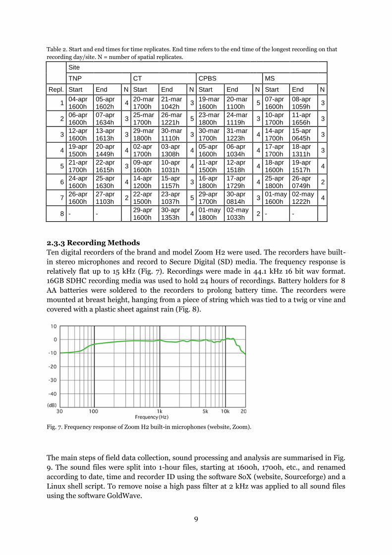
Table 2. Start and end times for time replicates. End time refers to the end time of the longest recording on that

recording day/site. N = number of spatial replicates.

Site

TNP

CT

CPBS MS

Repl. Start End N Start End N Start End N Start End N

1 04-apr 1600h

05-apr 1602h

4 20-mar 1700h

21-mar 1042h

3 19-mar 1600h

20-mar 1100h

5 07-apr 1600h

08-apr 1059h

3

2 06-apr 1600h

07-apr 1634h

3 25-mar 1700h

26-mar 1221h

5 23-mar 1800h

24-mar 1119h

3 10-apr 1700h

11-apr 1656h

3

3 12-apr 1600h

13-apr 1613h

3 29-mar 1800h

30-mar 1110h

3 30-mar 1700h

31-mar 1223h

4 14-apr 1700h

15-apr 0645h

3

4 19-apr 1500h

20-apr 1449h

4 02-apr 1700h

03-apr 1308h

4 05-apr 1600h

06-apr 1034h

4 17-apr 1700h

18-apr 1311h

3

5 21-apr 1700h

22-apr 1615h

3 09-apr 1600h

10-apr 1031h

4 11-apr 1500h

12-apr 1518h

4 18-apr 1600h

19-apr 1517h

4

6 24-apr 1600h

25-apr 1630h

4 14-apr 1200h

15-apr 1157h

3 16-apr 1800h

17-apr 1729h

4 25-apr 1800h

26-apr 0749h

2

7 26-apr 1600h

27-apr 1103h

2 22-apr 1500h

23-apr 1037h

5 29-apr 1700h

30-apr 0814h

3 01-may 1600h

02-may 1222h

4

8 - - 29-apr 1600h

30-apr 1353h

4 01-may 1800h

02-may 1033h

2 - -

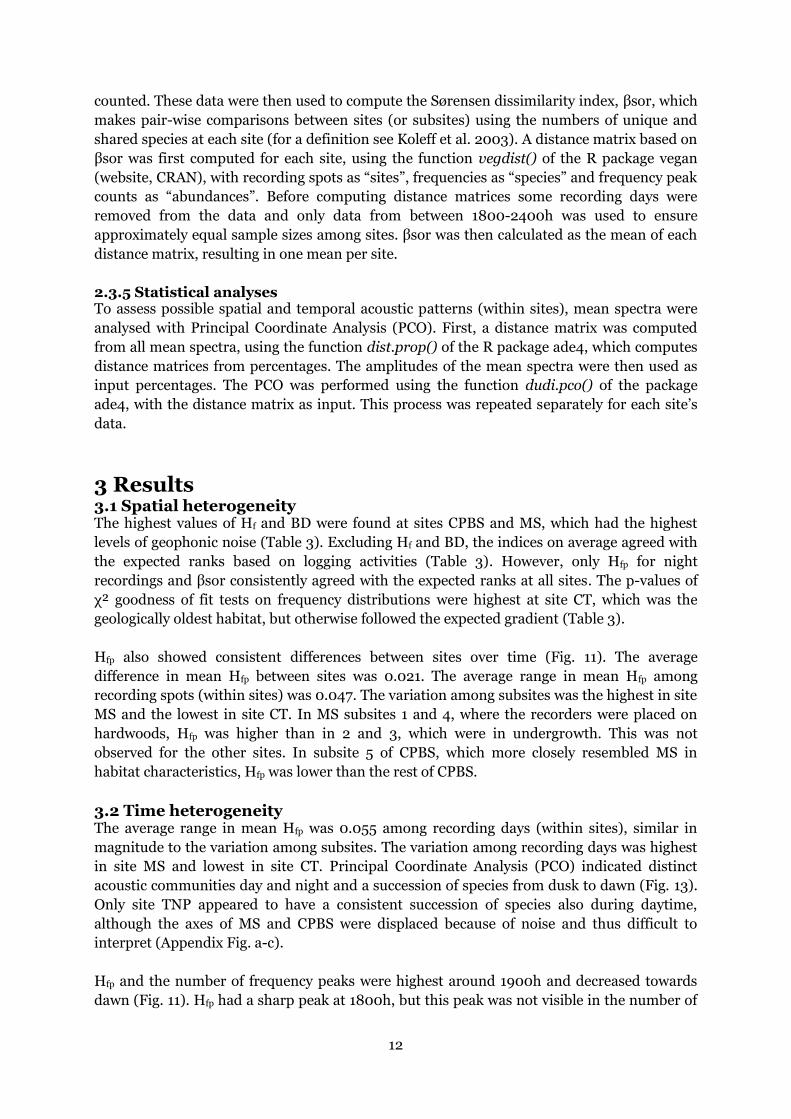
2.3.3 Recording Methods

Ten digital recorders of the brand and model Zoom H2 were used. The recorders have built-

in stereo microphones and record to Secure Digital (SD) media. The frequency response is

relatively flat up to 15 kHz (Fig. 7). Recordings were made in 44.1 kHz 16 bit wav format.

16GB SDHC recording media was used to hold 24 hours of recordings. Battery holders for 8

AA batteries were soldered to the recorders to prolong battery time. The recorders were

mounted at breast height, hanging from a piece of string which was tied to a twig or vine and

covered with a plastic sheet against rain (Fig. 8).

Fig. 7. Frequency response of Zoom H2 built-in microphones (website, Zoom).

The main steps of field data collection, sound processing and analysis are summarised in Fig.

9. The sound files were split into 1-hour files, starting at 1600h, 1700h, etc., and renamed

according to date, time and recorder ID using the software SoX (website, Sourceforge) and a

Linux shell script. To remove noise a high pass filter at 2 kHz was applied to all sound files

using the software GoldWave.

10

Fig. 8. Recorder field setup.

Fig. 9. Flowchart of the methodology used in this study. Metadata refers to date, time and location data.

2.3.4 Soundscape analyses Soundscape analyses were made in the statistical environment R with the packages “seewave”

(Sueur et al. 2008 B), “tuneR”, “ade4” and “vegan” (website, CRAN). The left stereo channel

of the first minute of every 10 minutes of recordings was loaded into R with the function

readWave() of TuneR. Each 1-minute segment was subjected to a “rain filter”. This original

filter consisted of two thresholds: A) minimum ratio between the peak amplitude and the

RMS amplitude and B) maximum RMS amplitude. A threshold of 0.045 was selected for A

and 68 for B. These thresholds were estimated by selecting 150 sound samples from the data

with or without rain and manually adjusting the thresholds to remove as many rain samples

as possible, while retaining most rain-free samples. Loud thuds caused by rain drops hitting

the plastic covering the recorders allowed rain to be easily identified and removed using this

filter. Mean frequency spectra were then computed for the remaining segments with the

function meanspec() of seewave, with a window length of 512 samples.

11

The Acoustic Entropy Index (H) is based on the Shannon index and consists of two

components: the temporal entropy, Ht, and spectral entropy, Hf (Sueur et al. 2008 A). Only

Hf was used in this study because tropical recordings usually have a flat amplitude envelope,

making Ht irrelevant (Jerome Sueur pers. com.). Hf was computed using the function sh() of

the package seewave with the mean frequency spectra as input.

Villanueva-Rivera et al. (2011) used a modification of Hf, which uses a specified set of

frequency bands to compute the index. I will refer to this index as Band Diversity (BD).

Villanueva-Rivera et al. (2011) provided an R-script that calculates the proportion of dB

values over a specified amplitude threshold occurring in each frequency band. These

proportions are then used to compute a Shannon index. I used the same R-script to compute

the band diversity, with 22 frequency bands (0 – 22050 kHz), a bandwidth of 1000 Hz and

an amplitude threshold of -50 dB.

The function fpeaks() of the package seewave detects frequency peaks, i.e. amplitude peaks

along the frequency axis, with a sensitivity specified by an amplitude slope threshold and

outputs the number of frequency peaks, their respective frequencies and relative amplitudes.

I selected an amplitude slope threshold of 0.01, which detected the most pronounced peaks

and eliminated peaks due to background noise. Fig. 10 shows an example from a 30-second

dawn recording. Additional indices were computed using the frequency peak data. The index

Hfp was computed similarly to Hf, using the function sh(). The number of categories that

were used to compute the Hfp index was not constant, making it a “true” diversity index,

unlike Hf and BD which are essentially evenness indices (Jerome Sueur pers. com.). Pielou's

evenness (Pielou 1966) for the frequency peaks was obtained by dividing Hfp by the log of the

number of frequency peaks.

Fig. 10. Example of a frequency peak plot (left) with the corresponding spectrogram (right) of a 30-second dawn recording. Red circles indicate the “counted” frequency peaks.

The uniformity of the frequency distribution among frequency peaks was tested with with a

χ² goodness of fit test on the consecutive distances (in kHz) between frequency peaks.

To estimate beta diversity within sites, frequency peaks were first rounded to Hz and

12

counted. These data were then used to compute the Sørensen dissimilarity index, βsor, which

makes pair-wise comparisons between sites (or subsites) using the numbers of unique and

shared species at each site (for a definition see Koleff et al. 2003). A distance matrix based on

βsor was first computed for each site, using the function vegdist() of the R package vegan

(website, CRAN), with recording spots as “sites”, frequencies as “species” and frequency peak

counts as “abundances”. Before computing distance matrices some recording days were

removed from the data and only data from between 1800-2400h was used to ensure

approximately equal sample sizes among sites. βsor was then calculated as the mean of each

distance matrix, resulting in one mean per site.

2.3.5 Statistical analyses To assess possible spatial and temporal acoustic patterns (within sites), mean spectra were

analysed with Principal Coordinate Analysis (PCO). First, a distance matrix was computed

from all mean spectra, using the function dist.prop() of the R package ade4, which computes

distance matrices from percentages. The amplitudes of the mean spectra were then used as

input percentages. The PCO was performed using the function dudi.pco() of the package

ade4, with the distance matrix as input. This process was repeated separately for each site’s

data.

3 Results 3.1 Spatial heterogeneity The highest values of Hf and BD were found at sites CPBS and MS, which had the highest

levels of geophonic noise (Table 3). Excluding Hf and BD, the indices on average agreed with

the expected ranks based on logging activities (Table 3). However, only Hfp for night

recordings and βsor consistently agreed with the expected ranks at all sites. The p-values of

χ² goodness of fit tests on frequency distributions were highest at site CT, which was the

geologically oldest habitat, but otherwise followed the expected gradient (Table 3).

Hfp also showed consistent differences between sites over time (Fig. 11). The average

difference in mean Hfp between sites was 0.021. The average range in mean Hfp among

recording spots (within sites) was 0.047. The variation among subsites was the highest in site

MS and the lowest in site CT. In MS subsites 1 and 4, where the recorders were placed on

hardwoods, Hfp was higher than in 2 and 3, which were in undergrowth. This was not

observed for the other sites. In subsite 5 of CPBS, which more closely resembled MS in

habitat characteristics, Hfp was lower than the rest of CPBS.

3.2 Time heterogeneity The average range in mean Hfp was 0.055 among recording days (within sites), similar in

magnitude to the variation among subsites. The variation among recording days was highest

in site MS and lowest in site CT. Principal Coordinate Analysis (PCO) indicated distinct

acoustic communities day and night and a succession of species from dusk to dawn (Fig. 13).

Only site TNP appeared to have a consistent succession of species also during daytime,

although the axes of MS and CPBS were displaced because of noise and thus difficult to

interpret (Appendix Fig. a-c).

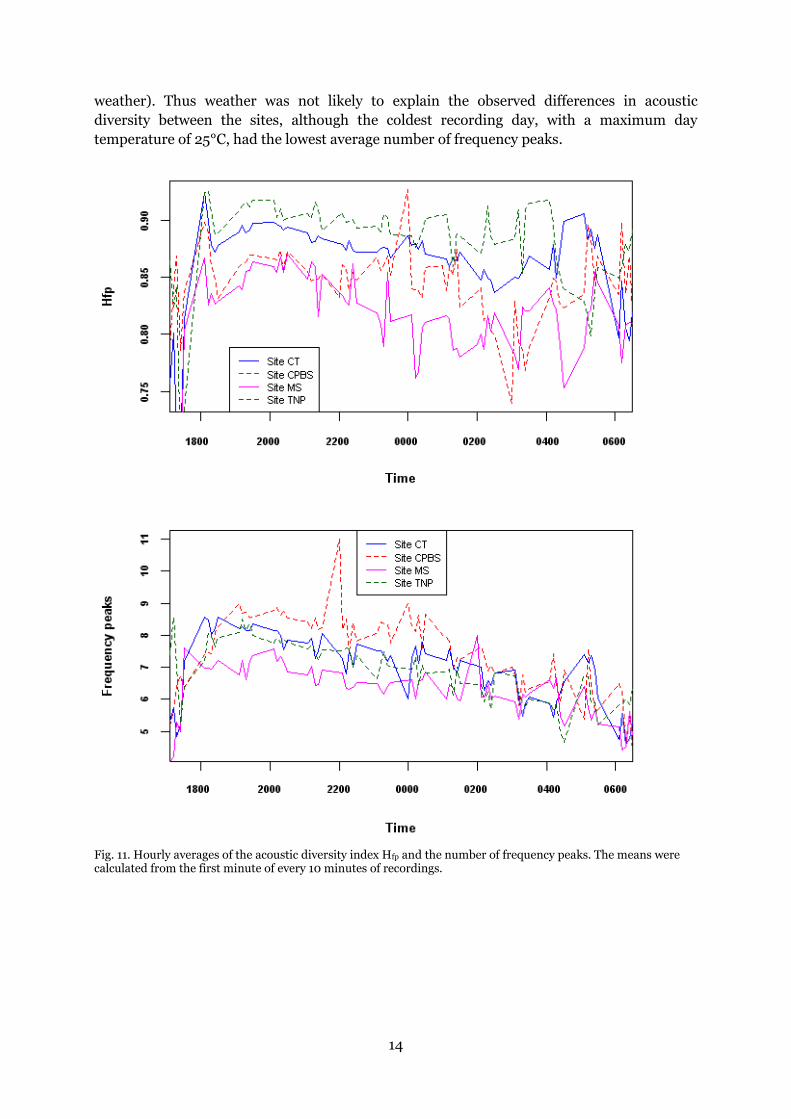
Hfp and the number of frequency peaks were highest around 1900h and decreased towards

dawn (Fig. 11). Hfp had a sharp peak at 1800h, but this peak was not visible in the number of

13

frequency peaks. Hf and BD generally increased during periods of low sound activity, except

at the peak of activity around 1900h where Hf showed similarly shaped curves to those of Hfp

(Fig. 12). BD also showed a small increase around 1900h for sites CT and TNP. After 2400h

data availability was too patchy to draw conclusions on smaller temporal scales.

Table 3. Mean of acoustic indices for four tropical wet forest sites. The sites were ranked 1-4 based on degree of

logging where 1=primary habitat and 4=extensively logged. Observed ranks within parentheses. * Lowest value

ranked highest.

Site TNP CT CPBS MS

Expected rank

1 2 3 4

Hfp Night 0.899 (1) 0.878 (2) 0.849 (3) 0.828 (4)

Day 0.845 (2) 0.831 (3) 0.855 (1) 0.811 (4)

Frequency peaks Night 7.25 (3) 7.46 (2) 7.95 (1) 6.62 (4)

Day 6.44 (1) 5.83 (3) 6.09 (2) 5.19 (4)

Pielou's evenness Night 0.464 (1) 0.446 (3) 0.420 (4) 0.450 (2)

Day 0.507 (4) 0.524 (3) 0.530 (2) 0.572 (1)

Hf Night 0.751 (4) 0.753 (3) 0.762 (1) 0.757 (2)

Day 0.824 (4) 0.828 (3) 0.853 (1) 0.839 (2)

Band diversity Night 0.068 (3) 0.065 (4) 0.075 (2) 0.086 (1)

Day 0.137 (2) 0.137 (4) 0.142 (1) 0.137 (3)

Freq. distribution χ²-test, Night 0.964 (2) 0.976 (1) 0.958 (3) 0.931 (4)

p-value Day 0.811 (1) 0.743 (2) 0.576 (4) 0.610 (3)

Freq. distribution χ²-test, Night 0.817 (2) 0.691 (1) 1.181 (4) 0.988 (3)

statistic * Day 1.786 (1) 2.487 (2) 4.377 (4) 2.487 (3)

Mean Sørensen dissimilarity

(βsor) 1800-2400h 0.313 (1) 0.283 (2) 0.251 (3) 0.236 (4)

3.3 Frequency components Nightly activity was concentrated to the 3-9 kHz frequency bands and was highest between 5-

7 kHz, while day recordings appeared to have a more flat frequency spectrum (Fig. 14). There

were very few frequency peaks above 12 kHz day or night, suggesting that the higher

frequency bands contained mostly wide-band signals and noise.

3.4 Weather 300 mm of rain fell during the field study period. Humidity was commonly 80-90% but

occasionally dropped below 60%. Average daily maximum and minimum temperatures were

31 and 20°C. The weather parameters had very similar means among sites (excluding the two

sites furthest away from the weather station, which were likely affected by local variation in

14

weather). Thus weather was not likely to explain the observed differences in acoustic

diversity between the sites, although the coldest recording day, with a maximum day

temperature of 25°C, had the lowest average number of frequency peaks.

Fig. 11. Hourly averages of the acoustic diversity index Hfp and the number of frequency peaks. The means were calculated from the first minute of every 10 minutes of recordings.

15

Fig. 12. Hourly averages of the acoustic diversity indices Hf and “BD”. The means were calculated from the first minute of every 10 minutes of recordings.

16

Fig. 13. Principal Coordinate Analysis (PCO) on mean frequency spectra. Mean spectra were computed from the first minute of every 10 minutes of recordings. Labels indicate the factor time (hours). Gray = day recording, black = night recording. The plot shows site CT only; see appendix Fig. a-c for the other sites.

Fig. 14. Average number of frequency peaks per frequency (left) and the average proportion of sound per

frequency band (right).

17

4 Discussion 4.1 Acoustic indices Soundscape recordings were made in four tropical wet forest habitats subjected to varying

degrees of logging in the past. This study was fostered by the study by Sueur et al (2008 A),

which found acoustic diversity as measured by the acoustic index “H” to be higher in the less

altered of two Tanzanian coastal forests. Here, two acoustic diversity indices, Hfp and βsor,

were used for the first time using sampling effort that was considerably larger than in Sueur

et al.’s (2008 A) study. Both indices decreased with higher degree of logging, supporting the

previous study by Sueur et al (2008 A), although different acoustic indices were used.

Periods of low acoustic activity during daytime increased the influence of background noise

and of single, noisy species such as cicadas. Because of this, daytime results were difficult to

interpret, and in the following discussion I will refer to night recordings unless specified

otherwise.

Hfp, as a Shannon index, has a “species richness” component and an evenness component

(relative abundances). The “species richness” of Hfp consists of the number of frequency

peaks which are expected to increase with the number of species present in a recording. The

evenness component is represented by Pielou’s index and measures the evenness of the

relative amplitudes of frequency peaks. It is, however, uncertain whether the relative

amplitudes reflect actual species abundances, since they are influenced by both signal

characteristics and the distance of the source to the microphone. Signal amplitude and

duration are species-specific and might be non-randomly distributed between sites, since

signals might be adapted to the physical properties of each habitat (Obrist et al. 2010,

Bormpoudakis et al. 2013). The average distance of a species’ individuals to the microphone

should decrease with abundance and consequently increase the relative amplitude of

frequency peaks generated by this species, but how this is eventually reflected in the evenness

is not evident; many individuals of different species singing close to the microphone should

cause a high evenness, but so should a situation where a few individuals are singing from far

away. Pielou’s evenness was unexpectedly high in the low diversity site (site MS), but

otherwise followed the expected gradient, which highlights this problem. Nonetheless, Hfp

agreed with the expected biodiversity gradient across all sites. Thus the number of frequency

peaks appears to compensate for the possible weaknesses in the measurement of evenness.

The number of frequency peaks was highest at the two sites of intermediate logging, which

suggests higher species diversity at these sites, but considering their lower within-habitat

beta diversity it is highly uncertain if it reflects the overall species diversity of the habitats.

Less effective acoustic partitioning could also cause the soundscape to appear more crowded;

the Acoustic Niche Hypothesis simply predicts that vocalising animals should minimise

interference, not that the number of simultaneous signals should be maximised. The number

of frequency peaks, when used as an independent index, should therefore be complemented

with some measure of acoustic partitioning.

The observed gradients of Hfp and βsor were similar (among sites); one potential explanation

for this is that they measure the same phenomenon. The Acoustic Niche Hypothesis predicts

more effective local habitat partitioning in primary habitat (Krause 1987). This should

increase within-habitat beta diversity, which was measured by βsor, and also cause the

community to better use available acoustic space, thus increasing the evenness among the

18

relative amplitudes of signals, which was measured by Hfp. I suggest that βsor should be

interpreted as a measure of spatial acoustic partitioning and Hfp primarily as a measure of

spatial acoustic partitioning and only secondarily as a measure of species diversity.

The results from χ² analyses on frequency distributions followed the expected biodiversity

gradient, except that site CT had higher values than site TNP, indicating that CT had a more

uniform frequency distribution. Since peak frequency is a species-specific trait, the frequency

distribution is a measure of community composition, rather than a measure of how locally

present species are distributed. The uniformity of the frequency distribution can then be

expected to reflect long-term habitat stability and evolutionary time. It is thus

complementary to the indices Hfp and βsor in describing the acoustic community.

The detection of frequency peaks is a simple form of signal recognition that is biased towards

narrow-band signals. In tropical night recordings this results in a bias towards the songs of

Gryllidae rather than Tettigoniidae, which generally have wide-band songs (Riede, 1993).

Most frequency peaks detected at night were in the 4-9 kHz range used by Gryllids (Riede,

1993). Hence the indicator value of Hfp and related indices in this study was dependent on the

indicator value of Gryllidae as a group. However, when species diversity does not vary much,

the acoustic optimisation of the whole community should be a more important factor in

determining the indices.

The indices Hf (Sueur et al. 2008) and “BD” (Villanueva-Rivera et al. 2011) were strongly

influenced by breaking wave noise from the sea and did not provide much useful information

in this study. Neither of the indices showed consistent differences in acoustic diversity

between the two “noise-free” sites, although BD was higher at site TNP between 1800-2400h.

The sensitivity of these indices, especially BD, to wide-band signals made them susceptible to

single, noisy species having a large influence on the results (Sueur et al, 2008). This was a

common problem in day recordings; BD had almost identical daytime means for all sites.

Also, the amplitude threshold of BD might have increased the effect of noise by selectively

removing noise from relatively clean recordings. Because of these weaknesses the Hf and BD

indices are not recommended for daytime recordings and should not be used near sea shores

or similar noise sources, including streams, roads and wind, which disqualifies them from

large-scale implementation in many areas.

4.2 Spatio-temporal heterogeneity There was large variation in acoustic diversity between recording days and between recording

spots (within sites) which shows the importance of both temporal and spatial replication.

Both microphone placement and local habitat variation should be considered in sampling

design, as well as differences due to changing weather conditions, season and time of day.

The minimum number of replicates probably varies depending on habitat heterogeneity,

community composition and diversity, and weather conditions. In contrast to taxonomic

surveys this makes acoustic diversity surveys easier to do in tropical wet forests, since they

are relatively a-seasonal and have a high and constant activity of vocalising animals.

The acoustic diversity – time curve proved useful when comparing recording sites. A

snapshot of the acoustic diversity, for example at the peak of the dusk chorus, might be

misleading because it does not take into account temporal partitioning. Effective temporal

partitioning should even out the number of simultaneous signals over time. Peak measures of

19

acoustic diversity should thus be complemented with a mean over some period of time.

Recordings were made near ground level and might not represent the combined diversity of

all forest layers, since the insect communities might be vertically stratified (Diwakar &

Balakrishnan, 2007). Considering that site MS had a very sparse upper canopy its diversity

was probably overestimated compared to the other sites. It is possible that the site had

retained some facultative canopy species which were now singing from the lower canopy,

further increasing the bias. How to representatively sample all forest layers is something for

further studies.

4.3 Cost-effectiveness Gardner et al. (2008) calculated taxonomic survey costs for a number of animal groups in an

Amazonian rainforest. Invertebrate survey costs minus salaries for field and laboratory

personnel were around $1000 - $3000 USD. The equivalent sum for this study was

approximately $2000, but this will be reduced as recording technology advances. Moreover,

the purchasing of sound recording equipment is a one-time cost and can be viewed as a long-

term investment, rather than as a running cost. Gardner et al. also calculated standardised

survey costs based on rarefaction curves; unfortunately this was not possible with my data.

Although soundscape recordings cannot replace a taxonomic survey, they can reveal

information about communities that would traditionally require sampling across multiple

taxonomic groups and thus involve high costs associated with hiring taxonomic experts

(Gardner et al., 2008). Such costs were entirely eliminated in this study.

The recording method used in this study represents a “semi-automated” design: I used push-

to-record handheld digital recorders, but left them to record unsupervised. At the time of the

study (2011) a handheld recorder of the type that was used was available for roughly 1/5 of

the price of an automated call recorder. The benefits of automated recorders include

scheduling of recording times, which enables unsupervised recording for long periods, and

automated tagging/time stamping of files. Scheduling is of limited usefulness when the

recorders have to be repeatedly moved around, such as when recording in many spots over a

large area. Automated tagging saves some labour but the same information can easily be

recorded manually. For similar surveys as in this study I consider the cost-effectiveness of

handheld digital recorders to be greater than that of automated call recorders, but the trade-

off between the one-time cost of recording equipment and the running cost of field technician

salaries need to be carefully considered (Penman et al. 2005). Also, using a lower sampling

rate such as 22 kHz should not remove any significant frequency peaks and will enable longer

recordings using cheaper equipment.

4.4 Implications for conservation management of the Tortuguero area Site TNP had the highest values of the acoustic indices Hfp and βsor, indicating an

undisturbed habitat with high species diversity. This primary habitat found in Tortuguero

National Park is “acoustically optimised” to harbour many vocalising animals while

minimising acoustic interference, and has a high conservation value (Krause 1987, Sueur et

al. 2008 A). Primary forest should generally be of highest conservation priority because it is

uncertain how many primary forest species can survive in secondary forest (Gardner et al.

2007).

Site CT had high values of the indices Hfp and βsor, but lower values than TNP. The site had,

20

however, the most uniform frequency distribution as indicated by χ² analysis. The results

could be explained by the fact that Cerro Tortuguero, although fragmented and selectively

logged, has a much older and more static habitat than the surrounding alluvial plain

(MINAET-SINAC 2004). This indicates that Cerro Tortuguero has an old community which

might be unique to the area and should consequently be of high conservation priority. The

remaining forest around the hill should be protected from further exploitation and be allowed

to recover from recent selective logging.

The site CPBS represented a selectively logged, regenerating forest. A high number of

frequency peaks indicated high species diversity, but the levels of acoustic partitioning

appeared to be low. The forest at Caño Palma Biological Station and similar habitat can then

possibly have species diversity comparable to that of Cerro Tortuguero and Tortuguero

National Park, but a lower conservation value because of a more altered habitat, and likely

fewer sensitive species.

The results from site MS indicate that the abundant Manicaria swamp forest has a much

lower acoustic diversity than the other forest types studied. The site was occasionally

completely quiet during daytime, in sharp contrast to site TNP which had a succession of

species between all hours of the day. Nonetheless, there was considerable acoustic activity at

night which shows that the Manicaria swamp forest has retained some diversity of singing

insects, especially on remaining hardwoods, and that it is not unimportant for biodiversity

conservation in the area.

4.5 Conclusions I have shown that acoustic surveys can be a cost-effective alternative to species inventories in

calculating diversity indices for tropical forest conservation. A number of conclusions and

practical advice can be drawn from the results of this study:

The index Hfp and the number of frequency peaks provide some indication of species

diversity, but should be complemented with other measures.

Spatial acoustic partitioning can be estimated by the acoustic indices βsor and Hfp, as

a potential indicator of habitat intactness.

The uniformity of the frequency distribution of frequency peaks can be estimated by a

χ² goodness of fit test, as a potential indicator of habitat age and intactness.

The applicability of the previously published acoustic indices Hf and BD is highly

limited because of their noise-sensitivity.

The period between 1800-2400h had a high and predictable acoustic diversity and

appeared to be the most suitable for recording. The diurnal variation is likely to be

different among seasons and depending on habitat and geographic location.

Recordings need to be extensively replicated in time and space to account for seasonal

and diurnal variation, weather induced variation, and local variation due to

microphone placement and local habitat heterogeneity.

Sueur et al. (2008 A) called for further studies to compare acoustic indices against real

species inventories of different organism groups and from different habitats. This would be

important in order to verify the indicator values of acoustic indices, but no such study has yet

been made to my knowledge. Possible seasonal, latitudinal, elevational, and vertical canopy

gradients in acoustic diversity should also be investigated for better sampling protocol

design.

21

5 Acknowledgements This study was conducted under a permit from Ministerio del Ambiente y Energía (MINAE),

Costa Rica with number ACTo-GASP-PIN-02-2011, and with support from the Canadian

Organisation for Tropical Education and Rainforest Conservation (COTERC). The study was

made possible thanks to a generous donation by Dr. Steven Furino and his family. I would

like to thank Dr. Jérôme Sueur (Muséum national d’Histoire naturelle, Paris, France) for

important supervision and support throughout the project. Thanks to Dr. Todd Lewis who

assisted in the field and provided experience and knowledge of the Tortuguero area. Thanks

to Dr. Folmer Bokma (Umeå university, EMG, Umeå, Sweden) who supervised this thesis.

Thanks to Dr. Kymberley Snarr of COTERC whose support during the initial stage helped

realise the project. Thanks to Amandine Gasc (Muséum national d’Histoire naturelle, Paris,

France) for support in acoustic analysis. Also thanks to the volunteers at Caño Palma

Biological Station for assistance in the field.

6 References Barlow, J., Gardner, T.A., Araujo, I.S., Avila-Pires, T.C.S., Bonaldo, A.B., Costa, J.E. et al.

2007. Quantifying the biodiversity value of tropical primary, secondary and plantation

forests. Proceedings of the National Academy of Sciences of the United States of America,

104: 18555–18560.

Bormpoudakis, D., Sueur, J., Pantis, J.D. 2013. Spatial heterogeneity of ambient sound at the

habitat type level: ecological implications and applications. Landscape Ecology, 28: 495–

506.

Brown, K. 1997. Diversity, disturbance, and sustainable use of Neotropical forests: insects as

indicators for conservation monitoring. Journal of Insect Conservation, 1: 25-42.

CRAN - Analysis of Ecological Data: Exploratory and Euclidean methods in Environmental

sciences. http://cran.r-project.org/web/packages/ade4/ 2013-06-01.

CRAN - tuneR: Analysis of music and speech. http://cran.at.r-

project.org/web/packages/tuneR/ 2013-06-01.

CRAN - vegan: Community Ecology Package. http://cran.r-

project.org/web/packages/vegan/ 2013-06-01.

Depraetere, M., Pavoine, S., Jiguet, F., Gasc, A., Duvail, S., Sueur, J. 2012. Monitoring animal

diversity using acoustic indices: Implementation in a temperate woodland. Ecological

Indicators, 13: 46-54.

Diwakar, S. & Balakrishnan, R. 2007. Vertical stratification in an acoustically communicating

ensiferan assemblage of a tropical evergreen forest in southern India. Journal of Tropical

Ecology, 23: 479–486.

Ficken, R.W., Ficken, M.S., Hailman, J.P. 1974. Temporal pattern shifts to avoid acoustic

interference in singing birds. Science, 183: 762–763.

Frommolt, K-H., Bardeli, R., Clausen, M., et al. 2008. Proceedings of the International

Expert meeting on IT-based detection of bioacoustical patterns, December 7th until

December 10th, 2007 at the International Academy for Nature Conservation (INA) Isle of

Vilm, Germany.

Gage, S.H., Napoletano, B., Cooper, M. 2001. Assessment of ecosystem biodiversity by

acoustic diversity indices. Journal of the Acoustical Society of America, 109: 2430.

Garcia Quesada, M., Sanchez, P., Poveda, L. & Otarola, M. 2006. Field checklist for plants

found at Cano Palma Biological Station, Tortugero National Park and the Barra del

22

Colorado area. Canadian Organisation for Tropical Education and Rainforest

Conservation. 26 pp.

Gardner, T.A., Barlow, J., Parry, L.W., & Peres, C.A. 2007. Predicting the Uncertain Future of

Tropical Forest Species in a Data Vacuum. Biotropica, 39: 25–30.

Gardner, T.A., Barlow, J., Araujo, I.S., Avila-Pires, T.C.S., Bonaldo, A.B., et al. 2008. The

cost-effectiveness of biodiversity surveys in tropical forests. Ecology Letters, 11: 139–150.

Gasc, A., Sueur, J., Pavoine, S., Pellens, R., Grandcolas, P. 2013. Biodiversity sampling using

a global acoustic approach: contrasting sites with microendemics in New Caledonia. PLoS

ONE, 8: e65311, e.

Gerhardt, H.C. 1994. The Evolution of Vocalization in Frogs and Toads. Annual Review of

Ecology, Evolution, and Systematics, 25: 293-324.

Jiménez, R.R., García Quesada, M.A., González Cordero, H. & Saénz Espinoza, R.A. 2011.

Evaluación Ecológica Rápida para el manejo compartido del Cerro Tortuguero.

Universidad Estatal a Distancia. Escuela de Ciencias exactas y naturales. Curso:

Formulación de Sistemas Nacionales de Conservación.

Kelso, D.P. 1965. A contribution to the ecology of a tropical estuary. MSc Thesis, University of

Florida.

Koleff, P., Gaston, K.J. & Lennon, J.J. 2003. Measuring beta diversity for presence-absence

data. Journal of Animal Ecology, 72: 367–382.

Krause, B. 1987. The Niche Hypothesis: How Animals Taught Us to Dance and Sing.

Krause, B. 1998. Into a wild sanctuary: a life in music and natural sound. Heyday Books,

Berkeley, 200 pp.

Krause, B. 2002 A. Wild soundscapes: discovering the voice of the natural world. Wild

Sanctuary Books, Berkeley.

Krause, B. 2002 B. Wild Soundscapes in the National Parks: An Educational Program Guide

to Listening and Recording. National Park Service, RM47.

Lawton, J.H., Bignell, D.E., Bolton, B., Bloemers, G.F., Eggleton, P., Hammond, P.M., Hodda,

M., Holt, R.D., Larsen, T.B., Mawdsley, N.A., Stork, N.E., Srivastava, D.S. & Watt, A. D.

1998. Biodiversity inventories, indicator taxa and effects of habitat modification in tropical

forest. Nature, 391: 72-76.

Lewis, T.R. 2009. Environmental Influences On The Population Ecology Of Sixteen Anuran

Amphibians In A Seasonally Flooded Neotropical Forest. Farnborough College of

Technology School of Applied and Health Sciences. Ph.D. Thesis.

Lewis, T. R., Grant, P. B. C., Feltham, J., Flilipiak, D., Mason, T., Figueroa, A. & Mayne, G.

2011. Herpetofauna found at Caño Palma Biological Station, Cerro Mountain and

Tortuguero area. Canadian Organisation for Tropical Education and Rainforest

Conservation. 8 pp.

Lewis, T. R., Grant, P. B. C., Garcia-Quesada, M., Ryall, C. & LaDuke, T. C. 2010. A botanical

study of Caño Palma Biological Station (Estación Biológica Caño Palma), Tortuguero,

Costa Rica. Brenesia, 74: 73-84.

MINAET-SINAC. 2004. Plan de manejo del Parque Nacional Tortuguero – Costa Rica.

Bermúdez, F. & Hernández, C. (Eds.). Guápiles, Limón.

Moritz, C., Richardson, K.S., Ferrier, S., Monteith, G.B., Stanisic, J., Williams, S.E. & Whiffin,

T. 2001 . Biogeographical concordance and efficiency of taxon indicators for establishing

conservation priority in a tropical rainforest biota. Proceedings of the Royal Society of

London B, 268: 1875-1881.

Myers, N., Mittermeier, R.A., Mittermeier, C.G., da Fonseca, G.A.B. & Kent, J. 2000.

Biodiversity hotspots for conservation priorities. Nature, 403: 853-858.

23

Myers, R. L. 1990. Palm swamps. In: Lugo, A. E., Brinson, M. & Brown, S. (Ed.). Ecosystems

of the World 15: Forested Wetlands. Elsevier, Oxford, 267-278.

Obando, V. 2007. Biodiversidad de Costa Rica en Cifras. Editorial INBio, Santo Domingo de

Heredia, Costa Rica.

Obrist, M.K., Pavan, G., Sueur, J., Riede, K., Llusia, D. & Marquez, R. 2010. Bioacoustics

approaches in biodiversity inventories. Abc Taxa, 8: 68-99.

Peay, K.G., Kennedy, P.G., Davies, S.J., Tan, S. & Bruns, T.D. 2010. Potential link between

plant and fungal distributions in a dipterocarp rainforest: community and phylogenetic

structure of tropical ectomycorrhizal fungi across a plant and soil ecotone. New

Phytologist, 185: 529–542.

Peet, R.K. 1974. The Measurement of Species Diversity. Annual Review of Ecology and

Systematics, 5: 285-307.

Pekin, B.K., Jung, J., Villanueva-Rivera, L.J., Pijanowski, B.C., Ahumada, J.A. 2012.

Modeling acoustic diversity using soundscape recordings and LIDAR-derived metrics of

vertical forest structure in a neotropical rainforest. Landscape Ecology, 27: 1513–1522.

Penman, T.D., Lemckert, F.L., Mahony, M.J. 2005. A cost-benefit analysis of automated call

recorders. Applied Herpetology, 2: 389-400.

Pielou, E.C. 1966. The measurement of diversity in different types of biological collections.

Journal of Theoretical Biology, 13: 131-144.

Pijanowski, B.C., Farina, A., Gage, S.H., Dumyahn, S.L. & Krause, B.L. 2011. What is

soundscape ecology? An introduction and overview of an emerging new science.

Landscape Ecology, 26: 1213–1232.

Putz, F.E., Zuidema, P.A., Synnott, T., Peña-Claros, M., Pinard, M.A., Sheil, D., Vanclay, J.K.,

Sist, P., Gourlet-Fleury, S., Griscom, B., Palmer, J. & Zagt, R. 2012. Sustaining

conservation values in selectively logged tropical forests: the attained and the attainable.

Conservation Letters, 5: 296–303.

Ralph, C. J., Widowson, M. J., Frey, R. I., Herrera, P.A., & O'Donnell, B.P. 2005. An Overview

of a Landbird Monitoring Program at Tortuguero, on the Caribbean Coast of Costa Rica.

pp. 831-838 in C. John Ralph and Terrell D. Rich, editors. Bird Conservation

Implementation and Integration in the Americas: Proceedings of the Third International

Partners in Flight Conference. 2002 March 20-24; Asilomar, California; Volume 2. Gen.

Tech. Rep. PSW-GTR-191. Albany, CA: Pacific Southwest Research Station, Forest Service,

U.S. Department of Agriculture.

Ricotta, C. 2004. Through the Jungle of Biological Diversity. Acta Biotheoretica, 53: 29–38.

Riede, K. 1993. Monitoring biodiversity: analysis of Amazonian rainforest sounds. Ambio, 22:

546–548.

Schäfer, R.M. 1977. Tuning of the world. Alfred Knopf, NY.

SINAC – Parque Nacional Tortuguero.

http://www.sinac.go.cr/AC/ACTo/PNTortuguero/Paginas/default.aspx 2013-06-01.

Smith, B. & Wilson, J. B. 1996. A consumer’s guide to evenness indices. Oikos, 76: 70–82.

Snaddon, J., Petrokofsky, G., Jepson, P. & Willis, K.J. 2013. Biodiversity technologies: tools

as change agents. Biology Letters, 9: 20121029.

Sourceforge: SoX - Sound eXchange. http://sox.sourceforge.net/ 2013-06-01.

Sueur, J. 2002. Cicada acoustic communication: potential sound partitioning in a multi-

species community from Mexico. Biological Journal of the Linnean Society, 75: 379–394.

Sueur, J., Pavoine, S., Hamerlynck, O., Duvail, S. 2008 A. Rapid Acoustic Survey for

Biodiversity Appraisal. PLoS ONE, 3: e4065.

24

Sueur, J., Aubin, T., Simonis, C. 2008 B. Seewave: a free modular tool for sound analysis and

synthesis. Bioacoustics, 18: 213-226.

Tuomisto, H. 2012. An updated consumer’s guide to evenness and related indices. Oikos, 121:

1203–1218.

UICN/ORCA. 1992. Estrategia de conservacion para el desarrollo sostenible de llanuras de

Tortuguero, Numero Propio 1180. Universidad Nacional, Costa Rica.

Widdowson, W. P., & Widdowson, M. J. 2000. Checklist to the birds of Tortuguero, Costa

Rica. Caribbean Conservation Corporation, San Jose, Costa Rica. Available online at

http://www.fs.fed.us/psw/topics/wildlife/birdmon/

landbird/tortuguero/tortchecklist.shtml. Last accessed January 6, 2005.

Villanueva-Rivera, L.J., Pijanowski, B.C., Doucette, J.S., Pekin, B.K. 2011. A primer of

acoustics for landscape ecologists. Landscape Ecology, 26: 1233–1246.

Wimmer, J., Towsey, M., Planitz, B., Williamson, I. & Roe, P. 2013. Analysing environmental

acoustic data through collaboration and automation. Future Generation Computer

Systems, 29: 560–568.

Zoom. http://www.zoom.co.jp/english/products/h2/mic.html 2013-06-01.

1

Appendix

Fig. a. Principal Coordinate Analysis (PCO) on mean frequency spectra from site CPBS. Mean spectra were computed from the first minute of every 10 minutes of recordings. Labels indicate the factor time (hours).

2

Fig. b. Principal Coordinate Analysis (PCO) on mean frequency spectra from site MS. Mean spectra were computed from the first minute of every 10 minutes of recordings. Labels indicate the factor time (hours).

3

Fig. c. Principal Coordinate Analysis (PCO) on mean frequency spectra from site TNP. Mean spectra were computed from the first minute of every 10 minutes of recordings. Labels indicate the factor time (hours).

Dept. of Ecology and Environmental Science (EMG)

S-901 87 Umeå, Sweden

Telephone +46 90 786 50 00

Text telephone +46 90 786 59 00

www.umu.se