rapid bridge deck joint repair investigation – phase iii
TRANSCRIPT

Rapid Bridge Deck Joint Repair Investigation – Phase IIIFinal ReportDecember 2020
Sponsored byFederal Highway AdministrationIowa Department of Transportation(InTrans Project 13-451)

About the Construction Management and Technology programThe mission of the Construction Management and Technology (CMAT) program is to improve the efficiency and cost-effectiveness of planning, designing, constructing, and operating transportation facilities through innovative construction processes and technologies.
About the Institute for TransportationThe mission of the Institute for Transportation (InTrans) at Iowa State University is to develop and implement innovative methods, materials, and technologies for improving transportation efficiency, safety, reliability, and sustainability while improving the learning environment of students, faculty, and staff in transportation-related fields.
Iowa State University Nondiscrimination Statement Iowa State University does not discriminate on the basis of race, color, age, ethnicity, religion, national origin, pregnancy, sexual orientation, gender identity, genetic information, sex, marital status, disability, or status as a US veteran. Inquiries regarding nondiscrimination policies may be directed to the Office of Equal Opportunity, 3410 Beardshear Hall, 515 Morrill Road, Ames, Iowa 50011, telephone: 515–294–7612, hotline: 515–294–1222, email: [email protected].
Disclaimer NoticeThe contents of this document reflect the views of the authors, who are responsible for the facts and the accuracy of the information presented herein. The opinions, findings and conclusions expressed in this publication are those of the authors and not necessarily those of the sponsors.
The sponsors assume no liability for the contents or use of the information contained in this document. This report does not constitute a standard, specification, or regulation.
The sponsors do not endorse products or manufacturers. Any trademarks or manufacturers’ names appear only because they are considered essential to the objective of the document.
Quality Assurance StatementThe Federal Highway Administration (FHWA) provides high-quality information to serve Government, industry, and the public in a manner that promotes public understanding. Standards and policies are used to ensure and maximize the quality, objectivity, utility, and integrity of its information. The FHWA periodically reviews quality issues and adjusts its programs and processes to ensure continuous quality improvement.
Iowa DOT Statements Federal and state laws prohibit employment and/or public accommodation discrimination on the basis of age, color, creed, disability, gender identity, national origin, pregnancy, race, religion, sex, sexual orientation or veteran’s status. If you believe you have been discriminated against, please contact the Iowa Civil Rights Commission at 800-457-4416 or the Iowa Department of Transportation affirmative action officer. If you need accommodations because of a disability to access the Iowa Department of Transportation’s services, contact the agency’s affirmative action officer at 800-262-0003.
The preparation of this report was financed in part through funds provided by the Iowa Department of Transportation through its “Second Revised Agreement for the Management of Research Conducted by Iowa State University for the Iowa Department of Transportation” and its amendments.
The opinions, findings, and conclusions expressed in this publication are those of the authors and not necessarily those of the Iowa Department of Transportation or the U.S. Department of Transportation Federal Highway Administration.

Technical Report Documentation Page
1. Report No. 2. Government Accession No. 3. Recipient’s Catalog No.
InTrans Project 13-451
4. Title and Subtitle 5. Report Date
Rapid Bridge Deck Joint Repair Investigation – Phase III December 2020
6. Performing Organization Code
7. Author(s) 8. Performing Organization Report No.
David Morandeira (orcid.org/0000-0002-1312-186X), Elizabeth Miller
(orcid.org/0000-0001-8796-3595), and Charles T. Jahren (orcid.org/0000-
0003-2828-8483)
InTrans Project 13-451
9. Performing Organization Name and Address 10. Work Unit No. (TRAIS)
Institute for Transportation
Iowa State University
2711 South Loop Drive, Suite 4700
Ames, IA 50010-8664
11. Contract or Grant No.
12. Sponsoring Organization Name and Address 13. Type of Report and Period Covered
Iowa Department of Transportation
800 Lincoln Way
Ames, IA 50010
Federal Highway Administration
1200 New Jersey Avenue, SE
Washington, DC 20590
Final Report
14. Sponsoring Agency Code
SPR RB33-013
15. Supplementary Notes
Visit https://intrans.iastate.edu/ for color pdfs of this and other research reports.
16. Abstract
The Iowa Department of Transportation (DOT) funded a three-phase research project focusing on rapid bridge deck joint repair.
Phase I focused on the documentation of current means and methods of bridge expansion joint maintenance and replacement.
Under Phase II, a workshop with Iowa DOT personnel, engineers, and researchers identified possible improvements to traditional
expansion joint options. From the workshop, a deck over backwall detail was developed that moved the expansion joint away
from the bridge deck and instead placed it on the approach slab. This would not only minimize the concrete removal needed for a
rehabilitation but would, in turn, prevent deicing chemicals from leaking through the deck joints and damaging the bridge’s
substructure. In Phase III, the research team was tasked with the further development of this deck over backwall concept.
Full-scale finite element (FE) models of two different bridges were developed to analyze the impact of the deck over backwall
concept. Both models were validated using the original drawing plans and American Association of State Highway and
Transportation Officials (AASHTO) specifications.
Through experimental testing and the development of FE models, two reinforcing options within the approach slab and
diaphragm sections were considered. The results showed that, when both the top and bottom longitudinal reinforcing was kept
continuous through the approach slab and diaphragm section, negative moment was transferred to the bridge deck. This transfer
of stress through the top reinforcing caused cracking to occur on the top of the bridge deck, which could lead to harmful
chemicals leaking onto the substructure. Conversely, experimental testing showed that these stresses could be eliminated if the
top longitudinal reinforcing and concrete cover were saw cut.
A plan for construction observation and post-construction testing was developed that included an instrumentation plan and
various real-world truck loading cases to be correlated with the FE models; an initial cost estimate was also developed.
Implementation of the deck over backwall concept and the post-construction plan is expected to be conducted in a future Iowa
DOT construction season.
17. Key Words 18. Distribution Statement
bridge joint repair—bridge maintenance—deck over backwall—design
details—expansion joint design—expansion joint replacement
No restrictions.
19. Security Classification (of this
report)
20. Security Classification (of this
page)
21. No. of Pages 22. Price
Unclassified. Unclassified. 207 NA
Form DOT F 1700.7 (8-72) Reproduction of completed page authorized


RAPID BRIDGE DECK JOINT REPAIR
INVESTIGATION – PHASE III
Final Report
December 2020
Principal Investigator
Charles T. Jahren, Professor
Construction Management and Technology
Institute for Transportation, Iowa State University
Research Assistants
David Morandeira and Elizabeth Miller
Authors
David Morandeira, Elizabeth Miller, and Charles T. Jahren
Sponsored by
Iowa Department of Transportation
Preparation of this report was financed in part
through funds provided by the Iowa Department of Transportation
through its Research Management Agreement with the
Institute for Transportation
(InTrans Project 13-451)
A report from
Institute for Transportation
Iowa State University
2711 South Loop Drive, Suite 4700
Ames, IA 50010-8664
Phone: 515-294-8103 / Fax: 515-294-0467
https://intrans.iastate.edu/


v
TABLE OF CONTENTS
ACKNOWLEDGMENTS .............................................................................................................xv
EXECUTIVE SUMMARY ........................................................................................................ xvii
CHAPTER 1. INTRODUCTION ....................................................................................................1
1.1 Problem Statement .........................................................................................................1 1.2 Background ....................................................................................................................1 1.3 Joint Detailing ................................................................................................................3
1.4 Objectives ......................................................................................................................6
CHAPTER 2. LITERATURE REVIEW .........................................................................................7
2.1 Repair, Replacement, and Elimination of Expansion Joints ..........................................7
2.2 Use of Ultra-High Performance Concrete for Bridge Joints ........................................16 2.3 Modeling and Analysis of Bridges ..............................................................................31
CHAPTER 3. FINITE ELEMENT MODELING AND ANALYSIS ...........................................43
3.1 Story County Bridge ....................................................................................................43
3.2 Marshall County Bridge ...............................................................................................62 3.3 Summary and Discussion ...........................................................................................112
CHAPTER 4. EXPERIMENTAL TESTING PLAN...................................................................116
4.1 Testing Objectives .....................................................................................................116 4.2 Testing Plan ...............................................................................................................117
4.3 Experimental Testing Results ....................................................................................124
4.4 Finite Element Modeling ...........................................................................................147
CHAPTER 5. COST ANALYSIS ...............................................................................................158
5.1 Background ................................................................................................................158
5.2 Service Life of Joints .................................................................................................159 5.3 Cost Estimate over Bridge Service Life.....................................................................161 5.4 Construction Cost of Deck over Backwall Concept ..................................................168
5.5 Break-Even Point Analysis ........................................................................................172 5.6 Summary and Discussion ...........................................................................................174
CHAPTER 6. CONSTRUCTION OBSERVATION AND POST-CONSTRUCTION
TESTING PLAN .............................................................................................................176
6.1 Joint Detailing ............................................................................................................176
6.2 Instrumentation ..........................................................................................................176 6.3 Truck Loading Cases .................................................................................................179
CHAPTER 7. CONCLUSIONS AND FUTURE WORK ...........................................................183
7.1 Joint Detailing ............................................................................................................183 7.2 Finite Element Modeling and Analysis......................................................................183 7.3 Experimental Investigation ........................................................................................184 7.4 Cost Analysis .............................................................................................................185 7.5 Construction Observation and Post-construction Testing..........................................186

vi
REFERENCES ............................................................................................................................187

vii
LIST OF FIGURES
Figure 1.1. Minimum concrete removal concept .............................................................................2
Figure 1.2. Deck over backwall concept ..........................................................................................2 Figure 1.3. Preliminary approach slab detail developed by the Iowa DOT .....................................3 Figure 1.4. Preliminary approach slab detail with option of saw cut and seal ................................4 Figure 1.5. Concrete removal process for Iowa DOT joint .............................................................5 Figure 1.6. Plan view of Iowa DOT joint ........................................................................................6
Figure 2.1. Integral abutment cross-section .....................................................................................9 Figure 2.2. New York semi-integral abutment cross-section ........................................................10 Figure 2.3. Debonded link slab system ..........................................................................................11 Figure 2.4. NYSDOT deck extension detail ..................................................................................13 Figure 2.5. MDOT deck extension detail .......................................................................................14
Figure 2.6. MDOT sleeper slab detail ............................................................................................15 Figure 2.7. Sherbrooke Pedestrian Bridge, Quebec, Canada (1997) .............................................17
Figure 2.8. Mars Hill Bridge, Wapello County, Iowa (2006) ........................................................18 Figure 2.9. Jakway Park Bridge, Buchanan County, Iowa (2008) ................................................18
Figure 2.10. Cross-section of pi-shaped girder ..............................................................................19 Figure 2.11. Typical section through a transverse, full-depth precast panel joint .........................20 Figure 2.12. Route 31 over Canandaigua Outlet - deck bulb-tee in place before UHPC
placement ......................................................................................................................21 Figure 2.13. Route 23 over Otego Creek in Oneonta - precast deck placement in progress .........22
Figure 2.14. Route 42 over West Kill - panel joint placement in progress....................................23 Figure 2.15. I-81 over East Castle St. - precast deck placement in progress .................................24 Figure 2.16. NYSDOT link slab cross-section ..............................................................................25
Figure 2.17. Finished NYSDOT link slab .....................................................................................26
Figure 2.18. Circle Interchange Project - UHPC transverse joint..................................................27 Figure 2.19. Circle Interchange Project - UHPC longitudinal joint ..............................................27 Figure 2.20. Circle Interchange Project - shear stud pocket ..........................................................28
Figure 2.21. Pulaski Skyway - typical transverse joint ..................................................................29 Figure 2.22. Pulaski Skyway - typical shear pocket detail ............................................................30 Figure 2.23. Pulaski Skyway - typical median detail.....................................................................31
Figure 2.24. Full 3D finite element model .....................................................................................33 Figure 2.25. Vårby Bridge 2010 - steel girders .............................................................................34 Figure 2.26. Vårby Bridge 2010 - concrete deck ...........................................................................34 Figure 2.27. Vårby Bridge 2010 - full 3D FE model .....................................................................35 Figure 2.28. Vårby Bridge 2015 - beam elements .........................................................................35
Figure 2.29. Vårby Bridge 2015 - main girders .............................................................................36
Figure 2.30. Vårby Bridge 2010 - boundary condition MPC ........................................................37
Figure 2.31. Vårby Bridge 2015 - main girder constraints ............................................................38 Figure 2.32. Vårby Bridge 2015 - crossbeam constraints ..............................................................38 Figure 2.33. Vårby Bridge 2015 - deck and main girder constraints .............................................39 Figure 2.34. Section view of approach slab modeling ...................................................................40 Figure 2.35. Boundary conditions for approach slab modeling .....................................................41 Figure 2.36. Trench geometry for approach slab modeling ...........................................................41 Figure 3.1. Story County bridge - full 3D FE model .....................................................................43

viii
Figure 3.2. Story County bridge - section view .............................................................................44 Figure 3.3. Story County bridge - steel superstructure ..................................................................44
Figure 3.4. Story County bridge - boundary conditions ................................................................45 Figure 3.5. Story County bridge - mesh convergence study ..........................................................46 Figure 3.6. Story County bridge - anticipated dead load deflection ..............................................47 Figure 3.7. Story County bridge - deformation contour plot for dead load ...................................48 Figure 3.8. Story County bridge - deformation contour plot for temperature loading ..................49
Figure 3.9. HS20-44 loading conditions and tire spacing ..............................................................50 Figure 3.10. HS20-44 loading conditions and uniform live load ..................................................50 Figure 3.11. Story County bridge - full 3D VBridge model ..........................................................51 Figure 3.12. Story County bridge - controlling truck loading conditions for abutment
reactions ........................................................................................................................52
Figure 3.13. Story County bridge - controlling truck loading conditions for pier reactions .........52
Figure 3.14. Story County bridge - controlling truck loading conditions for deflection ...............53 Figure 3.15. Controlling lane load for abutment reactions ............................................................53
Figure 3.16. Controlling lane load for pier reactions .....................................................................53
Figure 3.17. Controlling lane load for deflection ..........................................................................53 Figure 3.18. Story County bridge - load allocation for deflection .................................................54 Figure 3.19. Story County bridge - deformation contour plot for deflection truck load ...............54
Figure 3.20. Story County bridge - load allocation for abutment reactions ..................................55 Figure 3.21. Story County bridge - deformation contour plot for abutment reactions truck
load ................................................................................................................................56 Figure 3.22. Truck loading conditions from the drawing plans .....................................................57 Figure 3.23. Story County bridge - updated load allocation for abutment reactions .....................58
Figure 3.24. Story County bridge - load allocation for pier reactions ...........................................60
Figure 3.25. Story County bridge - deformation contour plot for pier reactions truck load ..........60 Figure 3.26. Story County bridge - updated load allocation for pier reactions .............................61 Figure 3.27. Marshall County bridge - gull 3D FE model .............................................................63
Figure 3.28. Marshall County bridge - plan view ..........................................................................63 Figure 3.29. Marshall County bridge - steel superstructure ...........................................................64
Figure 3.30. Marshall County bridge - boundary conditions .........................................................64 Figure 3.31. Marshall County bridge - mesh convergence study ..................................................66 Figure 3.32. Marshall County bridge - anticipated dead load deflection .......................................67
Figure 3.33. Marshall County bridge - deformation contour plot for dead load ...........................67 Figure 3.34. Marshall County bridge - deformation contour plot for temperature loading ...........69 Figure 3.35. Marshall County bridge - full 3D VBridge model ....................................................70
Figure 3.36. Marshall County bridge - plan view of VBridge model ............................................70 Figure 3.37. Marshall County bridge - controlling truck loading conditions for abutment
reactions ........................................................................................................................71 Figure 3.38. Marshall County bridge - controlling truck loading conditions for pier
reactions ........................................................................................................................71 Figure 3.39. Marshall County bridge - controlling truck loading conditions for deflection .........72 Figure 3.40. Marshall County bridge - load allocation for deflection ...........................................73
Figure 3.41. Marshall County bridge - deformation contour plot for deflection truck load ..........73 Figure 3.42. Marshall County bridge - load allocation for abutment reactions .............................74

ix
Figure 3.43. Marshall County bridge - deformation contour plot for abutment reactions
truck load .......................................................................................................................75
Figure 3.44. Marshall County bridge - updated load allocation for abutment reactions ...............76 Figure 3.45. Marshall County bridge - load allocation for pier reactions ......................................77 Figure 3.46. Marshall County bridge - deformation contour plot for pier reactions truck
load ................................................................................................................................77 Figure 3.47. Marshall County bridge - updated load allocation for pier reactions ........................78
Figure 3.48. Full 3D FE model with approach slab .......................................................................80 Figure 3.49. Section view without end span beam ........................................................................80 Figure 3.50. Section view with end span beam .............................................................................81 Figure 3.51. Boundary conditions section view.............................................................................82 Figure 3.52. Boundary conditions 3D view ...................................................................................82
Figure 3.53. Contact interaction.....................................................................................................83
Figure 3.54. Dead load abutment reactions ...................................................................................85 Figure 3.55. Deformation contour plot for temperature loading ...................................................86
Figure 3.56. Case 1 - truck load allocation ....................................................................................86
Figure 3.57. Case 2 - truck load allocation ....................................................................................87 Figure 3.58. Case 3 - truck load allocation ....................................................................................87 Figure 3.59. Case 4 - truck load allocation ....................................................................................87
Figure 3.60. Live load abutment reactions.....................................................................................89 Figure 3.61. Midspan deflection values with soil support .............................................................91
Figure 3.62. Midspan deflection values without soil support ........................................................91 Figure 3.63. Abutment deflection values with soil support ...........................................................92 Figure 3.64. Abutment deflection values without soil support ......................................................92
Figure 3.65. Midspan top stress values with soil support ..............................................................94
Figure 3.66. Midspan top stress values without soil support .........................................................95 Figure 3.67. Midspan bottom stress values with soil support ........................................................95 Figure 3.68. Midspan bottom stress values without soil support ...................................................96
Figure 3.69. Abutment top stress values with soil support ............................................................96 Figure 3.70. Abutment top stress values without soil support .......................................................97
Figure 3.71. Abutment bottom stress values with soil support ......................................................97 Figure 3.72. Abutment bottom stress values without soil support .................................................98 Figure 3.73. Parametric study - non-skewed model ....................................................................100
Figure 3.74. Parametric study - 30° skew model .........................................................................100 Figure 3.75. Parametric study - 60° skew model .........................................................................100 Figure 3.76. Case 2 - non-skewed model .....................................................................................102
Figure 3.77. Case 2 - 30° skew model .........................................................................................103 Figure 3.78. Case 2 - 60° skew model .........................................................................................103
Figure 3.79. Parametric study - live load abutment reactions with soil support ..........................105 Figure 3.80. Parametric study - live load abutment reactions without soil support .....................105 Figure 3.81. Parametric study - midspan deflection values with soil support .............................107 Figure 3.82. Parametric study - midspan deflection values without soil support ........................107 Figure 3.83. Parametric study - abutment deflection values with soil support ............................108
Figure 3.84. Parametric study - abutment deflection values without soil support .......................108 Figure 3.85. Parametric study - midspan stress values with soil support ....................................110 Figure 3.86. Parametric study - midspan stress values without soil support ...............................110

x
Figure 3.87. Parametric Study - abutment stress values with soil support ..................................111 Figure 3.88. Parametric study - abutment stress values without soil support ..............................111
Figure 4.1. Laboratory test setup for Test 1 and Test 2 ...............................................................117 Figure 4.2. Laboratory specimen after concrete for approach slab and diaphragm sections
was placed, with steel girders visible ..........................................................................118 Figure 4.3. Construction joint at interface of existing bridge deck and concrete diaphragm
sections ........................................................................................................................119
Figure 4.4. Jack hammering performed on construction joint to increase bond strength ............121 Figure 4.5. Reinforcing strain gage layout...................................................................................122 Figure 4.6. Concrete strain gage (BDI) layout .............................................................................123 Figure 4.7. BDIs on laboratory specimen ....................................................................................123 Figure 4.8. String pot (displacement meter) layout .....................................................................124
Figure 4.9. General loading with load steps for Test 1 ................................................................125
Figure 4.10. Gridded laboratory specimen for cracking documentation .....................................126 Figure 4.11. Cracking on the top of the slab, Test 1 ....................................................................126
Figure 4.12. Cracking at the construction joint............................................................................127
Figure 4.13. Cracking on the bottom of the slab, Test 1 ..............................................................128 Figure 4.14. Cracking on the north side of the slab, Test 1 .........................................................128 Figure 4.15. Cracking on the south side of the slab, Test 1 .........................................................128
Figure 4.16. Cracking occurring in the concrete diaphragm section at the intersection with
the steel girder, Test 1 .................................................................................................129
Figure 4.17. Load-deflection curve at midspan of the approach slab, Test 1 ..............................130 Figure 4.18. Magnitude of strain in the reinforcing at 16 kips per loading area, with a focus
on the gages in concrete diaphragm, Test 1 ................................................................131
Figure 4.19. Load versus strain curve for BDIs on the top surface of the concrete
diaphragm, Test 1 ........................................................................................................132 Figure 4.20. Load versus strain curve for BDIs on the bottom surface of the concrete
diaphragm, Test 2 ........................................................................................................132
Figure 4.21. Magnitude of strain in reinforcing at 16 kips per loading area, with a focus on
the gages at the midspan of the approach slab, Test 1 ................................................133
Figure 4.22. Load versus strain for BDIs at the first third point on the approach slab, Test 1 ....134 Figure 4.23. Load versus strain for BDIs at the midspan on the approach slab, Test 1 ..............134 Figure 4.24. Load versus strain for BDIs at the second third point on the approach slab,
Test 1 ...........................................................................................................................135 Figure 4.25. General loading with load steps for Test 2 ..............................................................136 Figure 4.26. Saw cut at the top of the approach slab through the top reinforcing in
preparation for Test 2 ..................................................................................................137 Figure 4.27. Cracking on the north side of the slab, Test 2 .........................................................137
Figure 4.28. Cracking on the south side of the slab, Test 2 .........................................................137 Figure 4.29. Propagation of cracks occurring near midspan of approach slab, Test 2 ................138 Figure 4.30. Crushing occurring at the midspan of the approach slab at failure, Test 2 .............139 Figure 4.31. Sequence showing the propagation of cracking occurring above the hard
support until failure, Test 2 .........................................................................................140
Figure 4.32. Load-deflection curve at the midspan of the approach slab, Test 2 ........................141 Figure 4.33. Deflection along the length of the specimen at the truck loading condition and
failure, Test 2 ..............................................................................................................142

xi
Figure 4.34. Horizontal movement of the slab at the roller support, Test 2 ................................143 Figure 4.35. Side view of the deflection of the specimen and the rotation at the beginning
of the approach slab, Test 2.........................................................................................143 Figure 4.36. Reinforcing strain gage magnitudes at 16 kips per loading area .............................144 Figure 4.37. Load versus strain curve for BDIs on the bottom surface of the concrete
diaphragm, Test 2 ........................................................................................................145 Figure 4.38. Load versus strain curve for BDIs on the top surface of the concrete
diaphragm, Test 2 ........................................................................................................145 Figure 4.39. Compression stress-strain curve ..............................................................................148 Figure 4.40. Tension stress-strain curve ......................................................................................149 Figure 4.41. Relationship between tension (a) and compression (b) stress-strain response
and damage..................................................................................................................150
Figure 4.42. Boundary conditions in both the Test 1 and Test 2 FE models ...............................151
Figure 4.43. Constraints and the unbonded construction joint in the FE model ..........................151 Figure 4.44. Test 2 FE model with added elements .....................................................................152
Figure 4.45. Comparison between the FE model and the experimental results for deflection
along the length of specimen, Test 1 ...........................................................................152 Figure 4.46. Tensile damage on the top of the specimen, Test 1 .................................................153 Figure 4.47. Tensile damage on the bottom of the specimen, Test 1 ..........................................153
Figure 4.48. Tensile damage on the top of the specimen, Test 2 .................................................153 Figure 4.49. Tensile damage on the bottom of the specimen, Test 2 ..........................................154
Figure 4.50. Strain (E11) in the concrete along the length of the specimen, Test 1 (top) and
Test 2 (bottom) ............................................................................................................155 Figure 4.51. Strain (E11) in the reinforcing along the length of the specimen, Test 1 (top)
and Test 2 (bottom) .....................................................................................................156
Figure 4.52. Cracking (a) and stress concentration (b) at the saw cut and hard support, Test
2 ...................................................................................................................................157 Figure 5.1. Marshall County bridge - 25 year service life, average cost, early service life ........162
Figure 5.2. Marshall County bridge - 25 year service life, average cost, average service life ....162 Figure 5.3. Marshall County bridge - 25 year service life, average cost, late service life ...........163
Figure 5.4. Marshall County bridge - 50 year service life, average cost, early service life ........163 Figure 5.5. Marshall County bridge - 50 year service life, average cost, average service life ....164 Figure 5.6. Marshall County bridge - 50 year service life, average cost, late service life ...........164
Figure 5.7. Break-even point - average cost, early service life ....................................................172 Figure 5.8. Break-even point - average cost, average service life ...............................................173 Figure 5.9. Break-even point - average cost, late service life ......................................................173
Figure 6.1. Surveying prism (left), total station (right) ................................................................177 Figure 6.2. Monitoring plate details .............................................................................................177
Figure 6.3. Monitoring plate distribution .....................................................................................178 Figure 6.4. Instrumentation plan ..................................................................................................179 Figure 6.5. Truck loading Case 1 .................................................................................................180 Figure 6.6. Truck loading Case 2 .................................................................................................180 Figure 6.7. Truck loading Case 3 .................................................................................................181
Figure 6.8. Truck loading Case 4 .................................................................................................181

xii
LIST OF TABLES
Table 2.1. Vårby Bridge 2010 - boundary conditions ...................................................................36
Table 2.2. Soil properties for approach slab modeling ..................................................................41 Table 3.1. Story County bridge - mesh convergence study ...........................................................46 Table 3.2. Story County bridge - abutment and pier reactions from the drawing plans ................47 Table 3.3. Story County bridge - dead load abutment and pier reactions ......................................48 Table 3.4. Story County bridge - expansion plate settings ............................................................49
Table 3.5. Story County bridge - dead load and live load abutment reactions ..............................56 Table 3.6. Story County bridge - dead load and updated live load abutment reactions ................59 Table 3.7. Story County bridge - dead load and live load pier reactions .......................................61 Table 3.8. Story County bridge - dead load and updated live load pier reactions .........................62 Table 3.9. Marshall County bridge - mesh convergence study......................................................65
Table 3.10. Marshall County bridge - abutment and pier reactions from the drawing plans ........66 Table 3.11. Marshall County bridge - dead load abutment and pier reactions ..............................67
Table 3.12. Marshall County bridge - expansion plate settings .....................................................68 Table 3.13. Marshall County bridge - dead load and live load abutment reactions ......................75
Table 3.14. Marshall County bridge - dead load and updated live load abutment reactions .........76 Table 3.15. Marshall County bridge - dead load and live load pier reactions ...............................78 Table 3.16. Marshall County bridge - Dead load and updated live load pier reactions .................79
Table 3.17. Dead load abutment reactions (kips) ..........................................................................84 Table 3.18. Case 1 - live load abutment reactions (kips) ...............................................................88
Table 3.19. Case 2 - live load abutment reactions (kips) ...............................................................88 Table 3.20. Case 3 - live load abutment reactions (kips) ...............................................................88 Table 3.21. Case 4 - live load abutment reactions (kips) ...............................................................89
Table 3.22. Case 1 - deflection values (in.) ...................................................................................90
Table 3.23. Case 2 - deflection values (in.) ...................................................................................90 Table 3.24. Case 3 - deflection values (in.) ...................................................................................90 Table 3.25. Case 4 - deflection values (in.) ...................................................................................90
Table 3.26. Case 1 - stress values (psi) ..........................................................................................93 Table 3.27. Case 2 - stress values (psi) ..........................................................................................93 Table 3.28. Case 3 - stress values (psi) ..........................................................................................94
Table 3.29. Case 4 - stress values (psi) ..........................................................................................94 Table 3.30. Parametric study - dead load abutment reactions (kips) ...........................................100 Table 3.31. Parametric study - dead load abutment reactions without soil support (kips) ..........101 Table 3.32. Parametric study - dead load abutment reactions with soil support (kips) ...............101 Table 3.33. Parametric study - temperature deformation ............................................................102
Table 3.34. Parametric study - Case 1 - live load abutment reactions (kips) ..............................104
Table 3.35. Parametric study - Case 2 - live load abutment reactions (kips) ..............................104
Table 3.36. Parametric study - Case 1 - deflection values (in.) ...................................................106 Table 3.37. Parametric Study - Case 2 - deflection values (in.) ..................................................106 Table 3.38. Parametric study - Case 1 - stress values (psi)..........................................................109 Table 3.39. Parametric study - Case 2 - stress values (psi)..........................................................109 Table 4.1. Reinforcing bar list .....................................................................................................120 Table 4.2. Compressive strength of concrete cylinders ...............................................................121 Table 4.3. Deflection along the length of the specimen at 16 kips per loading area, Test 1 .......130

xiii
Table 4.4. Comparison of continuity of strain in the reinforcing in Test 1 and Test 2 in the
concrete diaphragm section .........................................................................................146
Table 4.5. Concrete strain along approach slab at standard truck loading, Test 1 and Test 2 .....147 Table 5.1. Typical service life of joints .......................................................................................158 Table 5.2. Typical cost of joints...................................................................................................159 Table 5.3. Repairs or replacements over 25 years .......................................................................160 Table 5.4. Repairs or replacements over 50 years .......................................................................160
Table 5.5. Story County bridge - 25 year service life, 2% inflation rate .....................................165 Table 5.6. Story County bridge - 50 year service life, 2% inflation rate .....................................165 Table 5.7. Story County bridge - 25 year service life, 3% inflation rate .....................................165 Table 5.8. Story County bridge - 50 year service life, 3% inflation rate .....................................166 Table 5.9. Story County bridge - 25 year service life, 4% inflation rate .....................................166
Table 5.10. Story County bridge - 50 year service life, 4% inflation rate ...................................166
Table 5.11. Marshall County bridge - 25 year service life, 2% inflation rate .............................167 Table 5.12. Marshall County bridge - 50 year service life, 2% inflation rate .............................167
Table 5.13. Marshall County bridge - 25 year service life, 3% inflation rate .............................167
Table 5.14. Marshall County bridge - 50 year service life, 3% inflation rate .............................167 Table 5.15. Marshall County bridge - 25 year service life, 4% inflation rate .............................168 Table 5.16. Marshall County bridge - 50 year service life, 4% inflation rate .............................168
Table 5.17. Deck over backwall concept construction items.......................................................169 Table 5.18. Story County bridge - construction cost of deck over backwall concept .................169
Table 5.19. Marshall County bridge - construction cost of deck over backwall concept ............170 Table 5.20. Deck over backwall comparison, 25 year service life, 2% inflation rate .................170 Table 5.21. Deck over backwall comparison, 50 year service life, 2% inflation rate .................171
Table 5.22. Deck over backwall comparison, 25 year service life, 3% inflation rate .................171
Table 5.23. Deck over backwall comparison, 50 year service life, 3% inflation rate .................171 Table 5.24. Break-even point of deck over backwall concept .....................................................174


xv
ACKNOWLEDGMENTS
The authors would like to thank the Iowa Department of Transportation (DOT) for sponsoring
this research as well as the Federal Highway Administration for state planning and research
(Federal SPR Part II, CFDA 20.205) funds used for this project.
The authors would like to thank the technical advisory committee for this project, including
Dean Bierwagen, Mark Carter, Dan Cramer, Matt Johnson, Linda Narigon, James Nelson, Steve
Sandquist, Justin Sencer, and Wayne Sunday. A multitude of Iowa DOT personnel, too
numerous to list, were engaged on this project, and the authors would like to thank each of them
for their individual contributions.


xvii
EXECUTIVE SUMMARY
Bridge deck expansion joints are used to allow movement of the bridge deck due to thermal
expansion, dynamic loading, and other factors. More recently, expansion joints have been sealed
to prevent winter deicing chemicals and other corrosives applied to bridge decks from leaking
through the deck joints and damaging the bridge’s substructure. Expansion joints are often one of
the first components of a bridge deck to fail, and repairing or replacing expansion joints is
essential to extending the life of the bridge.
The Iowa Department of Transportation (DOT) funded a three-phase research project focusing
on rapid bridge deck joint repair. In the Phase I study, the research team focused on documenting
the current processes, means, and methods of bridge expansion joint deterioration, maintenance,
and replacement and on identifying improvements to joint design, maintenance, and replacement
based on the input gathered.
After maintenance and replacement strategies were identified, a workshop was held at the
Institute for Transportation at Iowa State University to develop ideas to better maintain and
replace expansion joints. Maintenance strategies were included in the discussion to explore ways
to extend the useful life of joints and thereby decrease the number of joints replaced in a year and
reduce traffic disruptions.
In the Phase II study, the research team focused on providing details about the types of failure
exhibited by expansion joints in Iowa, measures taken to repair and prevent these types of
failures, current construction methods used by contractors in Iowa, and hypothesized ways to
improve methods of expansion joint repair and maintenance.
A second workshop was held with an emphasis solely on the replacement of expansion joints.
Discussion topics included various methods of replacing joints, the possibility of using partial-
depth deck removals for replacements, the removal of existing reinforcing steel from the end of
the deck, and an alternative construction design that would eliminate the joint at the abutment
and move it to a less problematic location. This alternative design was named the deck over
backwall concept.
In this Phase III study, the deck over backwall concept was developed in detail. Full-scale finite
element (FE) models of two different bridges were developed to analyze the impact of the deck
over backwall concept. Both models were validated using the original drawing plans and
American Association of State Highway and Transportation Officials (AASHTO) specifications.
Further investigation using these full-scale models led to more design options within the deck
over backwall concept. Experimental testing was conducted with two reinforcing options within
the approach slab and diaphragm section. The results were then compared to smaller finite
element models that matched the testing setup.
The results showed that when the both the top and bottom longitudinal reinforcing was kept
continuous through the approach slab and diaphragm section, negative moment was transferred

xviii
to the bridge deck. This transfer of stress through the top reinforcing caused cracking to occur on
the top of the bridge deck that could lead to harmful chemicals penetrating the substructure.
Conversely, experimental testing showed that these stresses could be eliminated if the top
longitudinal reinforcing and concrete cover were saw cut.
In summary, through a cooperative effort with the Iowa DOT Office of Bridges and Structures
and Office of Construction and Materials, district bridge maintenance crews, and contractors, the
researchers on this project developed the deck over backwall design concept. Implementation of
the deck over backwall concept and the post-construction plan is expected to be conducted in a
future Iowa DOT construction season.

1
CHAPTER 1. INTRODUCTION
1.1 Problem Statement
Accelerated bridge construction (ABC) techniques are changing the way that bridges are built
across the US. Given the ever-increasing number of vehicles traveling over the nation’s roadway
infrastructure, reducing lane closure times has been identified as a key benefit of ABC
techniques and practices. In recent years, extensive research has been conducted on ABC.
However, less attention has been devoted to accelerated repair and replacement of bridge deck
expansion joints. For bridges requiring expansion joints, there is a need for accelerated
replacement techniques that would lengthen the life cycle of bridges in areas with high annual
average daily traffic (AADT) levels and limited time for lane closures.
Many aging multiple-span bridges utilize some form of expansion joint to properly counteract
thermal movement and other behaviors. These joints are also intended to prevent the passage of
winter deicing chemicals and other corrosives applied to bridge decks so that they do not
penetrate and damage the substructure components of the bridge. The majority of these
expansion joints require frequent repair and multiple replacements during the normal service life
of a bridge. Over the years, extensive research has been done to improve the longevity of these
joints but has met with limited success. The elimination of deck joints instead of repair or
replacement has been identified as a suitable and preferred option for bridges of moderate length,
especially those with high traffic loads and where there are limited or no detour possibilities.
Deck joints can be eliminated as part of an accelerated construction project that minimizes traffic
disruptions. When deck joints are eliminated, the possible penetration of deicing chemical-laden
water into the substructure components would be much less of a concern.
This three-phase project, Rapid Bridge Deck Joint Repair Investigation, was initiated to address
the acute need for further research into accelerated options for the repair, replacement, and
elimination of deteriorating bridge deck expansion joints in the state of Iowa and across the US.
1.2 Background
Phase I of this research project focused on documenting the current means and methods of bridge
expansion joint maintenance and replacement and then conducting a workshop whose objective
was to identify improvements to joint design, maintenance, and replacement. Phase II involved a
literature review of topics related to bridge deck expansion joints, including the types of joints
used or tested in other states, common and reported modes of failure in other states, integral
abutments and differences in their use among states, and methods of eliminating deck joints from
existing bridges, and surveys regarding the average life span of particular types of expansion
joints. Two workshops were held that emphasized the replacement of expansion joints.
Discussions during the workshops indicated that a desirable approach would be to develop a
design that would (1) minimize the amount of required concrete removal and (2) move the joint
away from the bridge deck at the abutment interface and instead place it on the approach slab. A
schematic cross-section of both concepts can be seen in in Figure 1.1 and Figure 1.2.

2
Miller and Jahren 2017
Figure 1.1. Minimum concrete removal concept
Miller and Jahren 2017
Figure 1.2. Deck over backwall concept
By minimizing the amount of concrete removed, as shown in the schematic cross-section in
Figure 1.1, schedule times can also be minimized. Concrete removal has been recognized as one
of the factors that most affects construction time during expansion joint replacement projects.
The other schematic cross-section, Figure 1.2, shows a precast or cast-in-place (CIP) panel that is
used to span the existing abutment backwall and relocate the joint onto the approach slab. By
using this concept, the joint is moved to a location where the possible penetration of deicing
chemical-laden water into the substructure components cannot occur and cause deterioration, and
its construction time can be comparable to that required for traditional joint replacements.

3
1.3 Joint Detailing
In Phases I, II, and III of this project, the researchers worked with engineers from the Iowa
Department of Transportation (DOT) to develop an appropriate detail for the deck over backwall
concept that would perform well under Iowa DOT standards. The researchers presented various
detailing options, including a cast-in-place approach slab, a precast slab, a sleeper slab, and
micropiles. Using the various options presented, the detail described below was developed by
Iowa DOT engineers in consideration of typical construction practices and preferences.
A section view of the preliminary detail developed is shown in Figure 1.3.
Iowa DOT
Figure 1.3. Preliminary approach slab detail developed by the Iowa DOT
As the figure shows, the initial detailing of the approach slab contains both top and bottom
longitudinal reinforcing, continuous through the diaphragm and into the bridge deck.
Additionally, reinforcing hoops are provided within the concrete diaphragm. The approach slab
is not connected to the backwall and can freely slide over the element.
While both the top and bottom reinforcing are shown as continuous in Figure 1.3, the Iowa DOT
provided the option of saw cutting either one or both of these longitudinal reinforcing elements.
This is shown in Figure 1.4.

4
Iowa DOT
Figure 1.4. Preliminary approach slab detail with option of saw cut and seal
In this figure, both the top and the bottom reinforcing are shown as being cut. The detail
identifies that after saw cutting, the joint should be sealed. This type of joint would aid the
performance of the deck, should the approach slab deflect a considerable amount. With
considerable deflection, the rotation of the approach slab would cause negative moment to be
transferred into the existing bridge deck. The saw cut and sealed joint would prevent this
moment and additional stresses from fully transferring to the existing bridge deck. This would
mitigate any extra cracking that may occur while also preventing any rotation of the deck that
might affect driver comfort.
Figure 1.3 also shows that a joint is to be provided a minimum of 17 ft 6 in. from the existing
bridge deck in the approach slab. Possible options for this joint could include a sleeper slab, a
subdrain, or the Iowa DOT’s EF, CF, or CD joints. A combination of these could also be
implemented.
Figure 1.5 details the concrete removal process that should occur to implement the detail
outlined in the previous figures.

5
Iowa DOT
Figure 1.5. Concrete removal process for Iowa DOT joint
Several important aspects critical to the performance of the joint are detailed. First, the figure
identifies that both the top and bottom longitudinal bars from the bridge deck should be protected
during the removal process. Keeping these bars ensures that their strength can be fully developed
in the new approach slab section. Second, the detail identifies that the minimum removal limit of
the bridge deck can be no less than 2 ft 6 in. Finally, the removal limits for the approach slab
should be approximately 20 ft, corresponding to the length of an Iowa DOT approach slab
section. The depths of the previously existing bridge deck, the concrete above the steel
diaphragm girders, and the new approach slab sections vary.
Figure 1.6 shows an example plan view of the joint developed by the Iowa DOT.

6
Iowa DOT
Figure 1.6. Plan view of Iowa DOT joint
The example plan view is provided for a skewed bridge. The reinforcing in both the longitudinal
and transverse directions of the approach slab is shown. Spacing for these bars is 1 ft in all
directions. Additionally, splice lengths for these bars are provided.
1.4 Objectives
The objectives of this research are as follows:
• Conduct a literature review on the repair, replacement, and elimination of bridge deck
expansion joints
• Further develop the deck over backwall concept with plans that conform to the design
concepts developed in previous phases of this project
• Create finite element (FE) models of selected bridges and study the impact of the concept on
the existing bridge structures
• Conduct experimental testing to evaluate the performance of the deck over backwall concept
• Compare the cost of application of the concept to that of other types of joints
• Develop a plan for construction observation and post-construction testing where the concept
can be further studied after implementation
By achieving these objectives, the deck over backwall concept will be furthered developed and
the Iowa DOT can confidently design and implement the concept.

7
CHAPTER 2. LITERATURE REVIEW
The research team conducted a review of the published literature on three relevant topics. The
first topic is the current practices and options for the accelerated repair and replacement of
expansion joints. Related to the first topic, the use of ultra-high performance concrete (UHPC) in
bridge joints and connections was reviewed. Finally, the various practices for modeling and
analyzing bridge structures and soil properties using commercial software were studied.
2.1 Repair, Replacement, and Elimination of Expansion Joints
A thorough review of the literature on accelerated methods of repair, replacement, and
elimination of expansion joints was conducted in Phases I and II of this research. In conjunction
with the Iowa DOT, Miller and Jahren (2014) conducted an investigation focused on determining
the best ways to rapidly repair and replace expansion joints in Iowa and other states. Their
findings were synthesized by Phares and Cronin (2015). The findings are discussed and
summarized in the following pages.
2.1.1 Joint Repair and Replacement
The literature review revealed that demolition and concrete cure times account for the longest
segments of construction time in expansion joint replacement projects (Miller and Jahren 2017).
Hydrodemolition was identified as an effective and quick way to remove concrete from the
surrounding areas of the expansion joint; however, it is costly, and runoff containing small
concrete particles is an issue that must be dealt with (Phares and Cronin 2015).
To repair or replace sliding plate expansion joints, Iowa DOT personnel stated that it would be
best to remove the joint entirely. The open space would be filled with new concrete while
leaving a flat gap between the abutment and deck for expansion and contraction of the bridge
(Miller and Jahren 2014). This method of replacement avoids any unnecessary traffic delay
(Phares and Cronin 2015) but allows the free flow of chemical-laden water into the substructure
below. Therefore, this is recommended as a temporary solution.
There are various methods of repair and replacement for strip seal and compression seal
expansion joints. These methods depend on the condition of the expansion joint mechanism in
question. The use of compressed air or pressurized water to remove debris from the joint is
acceptable as long as the seal or extrusion is not damaged. If the strip seal or compression seal is
damaged, it may need to be removed and cleaned, or a new seal could be installed. The new
section may be spliced in, or the entire length of the seal may be replaced (Miller and Jahren
2014). Miller and Jahren (2014) pointed out that a new section should not be spliced between
two existing sections due to buckling concerns.
Various methods were recognized to replace the compression seal armoring. The armoring can
be replaced by removing and replacing the existing concrete with new concrete for a flat riding
surface. However, the process takes several hours to complete. Miller and Jahren (2014) found

8
an alternative system that can be installed in as little as 30 minutes per lane if no repair of the
vertical face of the concrete is required. This system is an inverted strip seal called the Silicoflex
joint sealing system from RJ Watson, Inc. It is installed using adhesives instead of extrusions.
The system has to be installed against a clean, flat, vertical face below the damaged extrusion
(Miller and Jahren 2014).
Other types of joints were also considered in the literature review. Finger and modular expansion
joints were found to be repairable by replacing the damaged joint component. The effort required
for replacement is variable and depends on the specific circumstances. In some cases,
replacement is a straightforward process. If a torn neoprene gland is discovered, the entire joint
does not have to be replaced. A new neoprene gland can be installed after the damaged one is
removed (Miller and Jahren 2014).
Integral abutment joints were also investigated. Miller and Jahren (2014) found that possible
locations of damage can usually be found on the tire buffing and silicon sealant. To repair these
deteriorated items, missing pieces from the tire buffing are replaced and new silicon is poured
into the joint (Miller and Jahren 2014).
2.1.2 Joint Elimination
In Phase II of this research, Miller and Jahren (2017) found that most bridge engineers would
consider the best type of joint to be no joint. Through a survey distributed to all state highway
agencies in the US, Palle et al. (2012) similarly found that most state highway agencies sought to
eliminate joints wherever possible. Several noted that joint elimination was a goal for new bridge
designs (Palle et al. 2012). In their investigation, Miller and Jahren (2017) conducted a thorough
review of the literature for possible joint elimination options. Elimination options were found in
integral abutments, semi-integral abutments, and link slabs.
2.1.2.1 Integral Abutments
The trend for accelerated methods of repair and replacement of expansion joints seems to be
toward eliminating deck joints altogether by utilizing the integral abutment design. A few
agencies are using this design as their sole option for new construction (Baker Engineering
2006). It is for this reason that integral abutment bridges are becoming increasingly popular in
the US.
Integral abutments differ from the more traditional type of abutments, which are most commonly
known as stud abutments, in that they embed the ends of the bridge girders into the backwall. An
integral abutment moves along with the movement of the girders due to thermal loading,
dynamic loading, and other factors. The pile supports of the abutment deflect as necessary to
accommodate abutment movement. A cross-section of a typical integral abutment can be seen in
Figure 2.1.

9
Dunker and Abu-Hawash 2005, Mid-Continent Transportation Research Symposium, Iowa State University Center
for Transportation Research and Education
Figure 2.1. Integral abutment cross-section
Most states that employ the use of these abutments have reported that they are satisfied with their
performance. Maruri and Petro (2005) surveyed all transportation agencies in the US regarding
their use of integral abutment bridges. A large number of agencies responded to the survey,
providing a 79% response rate. The survey results indicated that the estimated number of in-
service integral abutment bridges increased by almost 200% from an estimated 4,000 integral
abutment bridges in 1995 to an estimated 13,000 or more integral abutment bridges in 2004
(Miller and Jahren 2017).
Since deicing chemicals and snowplows are widely used in the northern states of the US versus
the southern states, integral abutments are much more common in the former than the latter. The
survey results showed that the use of integral abutments will continue in the future, as 77% of the
respondents stated that they will continue to use integral abutments for bridges where it is
possible to do so. While most states reported that they were satisfied with the performance of
their integral abutment bridges, three states in particular deviated. Arizona encountered problems
with the bridges’ approach slabs, while Vermont encountered scour issues. These two states
abandoned the use of integral abutments for future bridges. The third state, Washington,
encountered seismic issues and decided to move forward with semi-integral abutments for
bridges under circumstances where integral abutments might have been considered.

10
2.1.2.2 Semi-integral Abutments
Semi-integral abutments were created as an alternative to integral abutments. This option
functions in many of the same ways as an integral abutment. These abutments have the ends of
the bridge girders embedded in the backwall. The semi-integral abutment also moves with the
movement of the girders due to thermal loading, dynamic loading, and other factors. The main
difference between the two is that for semi-integral abutments the entire backwall and girder
system is situated on bearings and allowed to slide over a fixed foundation (Miller and Jahren
2017). A typical cross-section for a semi-integral abutment can be seen in Figure 2.2.
Yannotti et al. 2005, Integral Abutment and Jointless Bridges 2005 FHWA Conference. Constructed Facilities
Center, College of Engineering and Mineral Resources
Figure 2.2. New York semi-integral abutment cross-section
In Iowa, semi-integral abutments are not often used for new bridge construction. Instead, semi-
integral abutments are used for joint retrofits where an integral abutment is not compatible with
the existing bridge design. Expansion joints across the states have been replaced with semi-
integral abutments, mitigating the concern about possible deicing chemical-laden water
penetrating the substructure components. While the use of semi-integral abutments has been
increasing, semi-integral abutments have received much less attention than integral abutments.
Semi-integral abutments have largely been used in unique situations where integral abutments do
not work well, such as bridges with large skew angles or high backwalls or those built on
difficult soil conditions (Miller and Jahren 2017). One common difficulty arises when bedrock is
close to the surface and piles cannot develop sufficient horizontal resistance to provide fixity for
the footing (Yanotti et al. 2005).

11
2.1.2.3 Link Slabs
While integral and semi-integral abutments are alternatives to eliminating expansion joints at the
abutment interface, options for eliminating expansion joints above the piers are also available.
Link slabs have been used in numerous projects across the US to replace expansion joints located
over bridge piers. Link slabs do exactly what the name says: link the existing bridge deck
between two girders over the pier supports.
Miller and Jahren (2017) explain that the stiffness of the continued deck is so small in
comparison to that of the girders that continuity is assumed not to be provided. This means that
the bridge will continue to act as a series of simply supported members, and thus the original
bridge design will not be affected. The link slab acts as a beam with a moment caused by the
rotation at the ends of the girders. To provide the necessary flexibility for the link slab, a portion
of the deck is debonded at the ends of the girders (Aktan et al. 2008). A typical cross-section of a
link slab can be seen in Figure 2.3, which shows the moment and rotation detailing.
Lam et al. 2008, Ministry of Transportation of Ontario
Figure 2.3. Debonded link slab system
Since link slabs have not been implemented to the same extent as other methods of bridge deck
joint repair, replacement, and elimination, there is a limited amount of knowledge in terms of
their performance when implemented. Miller and Jahren (2017) describe a pilot link slab that
was built in 1998 by the North Carolina DOT (NCDOT). The pilot link slab was instrumented,
monitored, and tested after implementation. Beam end rotations of 0.02 radians were taken into
account in the design of the link slab. The link slab was also meant to have fine cracks under
service loads. The maximum width of these fine cracks was designed to be 0.013 in.

12
At no point over the next year of monitoring did the link slab exceed the 0.02 radians of beam
end rotations. A crack wider than 0.013 in. was noticed in the middle of the link slab. This crack
had a width of 0.063 in., was present before live load testing, and did not widen during the tests.
It was ultimately believed that this crack was larger than designed due to localized debonding of
the reinforcement (Wing and Kowalsky 2005).
Michigan installed numerous link slabs in the early 2000s as part of several deck rehabilitation
projects across the state. Inspections of these bridges in 2006 yielded observations similar to
those made by Wing and Kowalsky (2005) during the NCDOT study discussed above. In every
link slab inspected, a full-depth crack was found approximately at the centerline of the pier,
regardless of whether a saw cut had been made at these locations. However, other than the
transverse cracking at the pier centerlines, little other cracking or damage was reported at the link
slab locations (Aktan et al. 2008).
Aktan et al. (2008) completed a detailed FE analysis that was used to predict how certain
parameters affect the performance of link slabs used in the state of Michigan. The investigated
design parameters of the link slab were as follows: the link slab debonded length with respect to
adjacent span lengths, girder height, adjacent span ratio, and support conditions. Several
conclusions were drawn from the FE results:
• The top and bottom layer of steel should be continuous throughout the link slab.
• Additional moment and axial loads should be considered in the design of link slabs to
account for thermal gradients.
• Saw cuts should be provided at the centerline of the pier and at each end of the link slab.
These saw cuts concentrate cracking in areas where the performance of the link slab would
not be diminished.
2.1.2.4 Deck over Backwall
Miller and Jahren (2017) held various workshops with the objective of identifying improvements
to bridge deck joint maintenance and replacement. Workshop participants came up with a
concept that eventually evolved into the deck over backwall concept shown in Chapter 1, Figure
1.2. Further review of the literature was conducted to study possible implementation of this
concept in other states.
According to a 2004 survey, approximately 3,900 bridges with deck extensions are currently in
use in the United States (Miller and Jahren 2017). This type of bridge is stated to be particularly
prominent in the northeastern region of the US as opposed to the midwestern and northern
regions, where full integral abutment designs are more common (Maruri and Petro 2005). The
New York State DOT (NYSDOT) in particular has been building bridges with deck extensions
since the 1980s or earlier (Alampalli and Yannotti 1998).
Alampalli and Yannotti (1998) detailed 105 deck extensions that were inspected by the
NYSDOT, 72 with concrete superstructures and 33 with steel superstructures. These bridges

13
were found to be performing as anticipated, with minor deck cracking being the only significant
problem. Miller and Jahren (2017) drew several conclusions regarding deck extensions,
including the following two:
• Steel structures are usually less prone to deck cracking than prestressed-concrete
superstructures.
• Performance typically worsens with increased skew or span length.
Miller and Jahren (2017) compared jointless bridges and other types of joints, mainly
compression seals, utilizing NYSDOT bridge inspection and inventory data. The results of the
analysis show that components of jointless bridges performed better than components of
compression seal bridges.
Construction details for a typical NYSDOT deck extension are shown in Figure 2.4.
Alampalli and Yannotti 1998
Figure 2.4. NYSDOT deck extension detail
Discussing the detail, Alampalli and Yannotti (1998) mentioned that the deck and approach slab
used to be included in a single placement, and the formed joint was merely a saw cut to promote
full-depth cracking at the correct location. The design of NYSDOT deck extensions has since
been changed. The approach slab and deck are placed separately now, eliminating the need for a
saw cut. This joint is provided to allow superstructure rotation with the bottom layer of
longitudinal deck steel continuous through the joint to keep the deck and approach slab from
separating (Alampalli and Yannotti 1998).

14
Other DOTs have also developed jointless bridge decks with deck extension details similar to
those of the NYSDOT joint and the concept introduced in the Phase II workshops for this study,
which eventually evolved into the deck over backwall concept.
The Michigan DOT (MDOT) has worked on developing jointless bridge decks to combat
deterioration of the leaking expansion joints. MDOT’s detailing is shown in Figure 2.5.
Aktan et al. 2008
Figure 2.5. MDOT deck extension detail
Various differences can be seen between the NYSDOT and MDOT joints:
• Location of the construction joint (in line with the center of the backwall for the NYDOT
joint; in line with inside edge of the backwall for the MDOT joint)
• Location of the continuous longitudinal reinforcing (bottom reinforcement for the NYSDOT
joint; top reinforcement for the MDOT joint)
• Incorporation of a sleeper slab in the MDOT joint
Miller and Jahren (2017) pointed out that continuing the top layer of reinforcing through the joint
should allow negative moment transfer across the construction joint as opposed to allowing the
joint to act as a hinge.
Approach slab standards differ between the Iowa DOT and MDOT. The Iowa DOT uses 20 ft
approach slabs, while MDOT only uses 20 ft approach slabs for bridges with integral and semi-
integral abutments. However, for deck extension details, MDOT extends the approach slab 5 ft
from the near edge of the backwall to rest on a sleeper slab. This sleeper slab is intended to help

15
mitigate possible settlement issues between the existing pavement and the new approach slab.
MDOT’s sleeper slab detailing can be seen in Figure 2.6.
Michigan DOT
Figure 2.6. MDOT sleeper slab detail
Western Michigan University (WMU) developed FE models to help MDOT to analyze its deck
extension details and further improve its designs. The difference between continuing the top
layer of steel reinforcement versus the bottom layer of steel reinforcement was of particular
interest. FE results showed that continuing the top layer of reinforcing caused the construction
joint to transfer negative moment, i.e., tensile stresses, at the top of the approach slab around the
construction joint. Continuing the bottom layer of longitudinal reinforcing caused the joint to act
as a hinge, eliminating the stresses at the construction joint but increasing the nominal positive
moment at the midpoint of the approach slab. Given the later situation, continuity of the bottom
layer of steel was preferred (Aktan et al. 2008).
Miller and Jahren (2017) agreed with this conclusion because cracking can be allowed on the
bottom side of the slab. Designing for the additional midspan moment is more achievable than
designing for negative moment capacity at the top of the deck, where cracking should be
prevented. A waterstop could be included in the construction joint to prevent the passage of
water and mitigate additional cracking (Miller and Jahren 2017).
The research team contacted MDOT staff to obtain more information about their experiences
with bridge extension. The following summarizes the key takeaways:
• The implemented deck extensions for MDOT achieved the objectives that the Iowa DOT is
seeking to accomplish.
• Future detailing will provide continuous bottom reinforcement.

16
• An approach slab will be poured after the deck to provide a cold joint in the abutment
interface.
• Settlements issues at the sleeper slab can cause a bump at the transition from the approach
slab to the highway pavement.
2.2 Use of Ultra-High Performance Concrete for Bridge Joints
Thirty years ago, a new technology called UHPC started being researched for use in bridge
design and construction. This new material offered very durable solutions but required new
shapes, new design codes and standards, and new precast fabrication methods and formworks
(Perry and Corvez 2016). The lack of design codes and standards increased the risk of
implementation for owners and designers. These limitations held the material back from growing
in use at a faster pace. Nonetheless, as a very young material, 30 years into research and 20 years
into development, acceptance has been growing as more research has been conducted. The
industry has been noticing the advantageous properties that the material possesses (Perry and
Corvez 2016).
2.2.1 Mechanical Properties
According to American Concrete Institute (ACI) Committee 239 – Ultra-High Performance
Concrete (2012), UHPC is “a cementitious, concrete material that has a minimum specified
compressive strength of 150 MPa (21.6 ksi) with specified durability, tensile ductility and
toughness requirements; fibers are generally included to achieve specified requirements.” UHPC
exhibits very high compression strength, improved tensile behavior, and sustained post cracking
strength (Ronanki et al. 2016). This high compression strength and improved tensile behavior
facilitate high bond strength and, as a result, a short development length for steel reinforcement.
This is fully explained in the Federal Highway Administration (FHWA) Technical Note Design
and Construction of Field-Cast UHPC Connections (Graybeal 2014).
Additionally, Fehling et al. (2015) explain that “compared with conventional normal- and high-
strength concretes with their capillary porosity, UHPC exhibits a much denser microstructure. It
has virtually no capillary pores and is therefore so impervious to liquids and gases that its
corrosion [potential for embedded reinforcing] is practically zero; it can serve as the wearing
course of a bridge deck without any additional protection against chlorides, alkalis, or deicing
salts.” The low permeability is attributed to the fine powders and chemical reactivity, which
create an extremely compact matrix and a small, discontinuous pore structure (Perry and Royce
2010). UHPC formulations often consist of a combination of portland cement, fine sand, silica
fume, high-range water-reducing admixture (HRWR), fibers (usually steel), and water. Small
aggregates are sometimes used, as well as a variety of chemical admixtures (Russell and
Graybeal 2013). The improved properties of UHPC provide such benefits as simplified
construction techniques, increased speed of construction, improved durability, reduced
maintenance, reduced service outages, minimum interruption of traffic, reduced element size and
complexity, extended usage life, and improved resiliency (Perry and Corvez 2016).

17
2.2.2 Implementation of UHPC in Bridges
The first use of UHPC in a North American bridge was in 1997 for construction of the
Sherbrooke Pedestrian Bridge in Quebec, Canada (Perry and Seibert 2013). This 197 ft clear
span bridge, shown in Figure 2.7, was constructed from six precast 3D space truss UHPC
elements, post-tensioned together on site.
Lafarge
Figure 2.7. Sherbrooke Pedestrian Bridge, Quebec, Canada (1997)
Russell and Graybeal (2013) explain that “[t]he structural concept consists of a space truss with a
top UHPC chord that serves as the riding surface, two UHPC bottom chords, and truss diagonals
that slope in two directions.”
In 2001, the FHWA initiated a research program to evaluate and introduce UHPC into the US
highway program (Graybeal 2008). The first UHPC highway bridge completed in North America
was the Mars Hill Bridge in Wapello County, Iowa (Bierwagen et al. 2006). The simple single-
span bridge, shown in Figure 2.8, comprises three 110 ft long, 45 in. deep, precast, prestressed
concrete modified Iowa bulb-tee beams topped with a CIP concrete bridge deck.

18
Bridge Engineering Center 2008
Figure 2.8. Mars Hill Bridge, Wapello County, Iowa (2006)
Each beam containes 47 0.6 in. diameter, low-relaxation prestressing strands and no shear
reinforcement (Russell and Graybeal 2013). The most significant aspect of this first UHPC
highway bridge was the use of the three UHPC I-girders without any stirrups for shear
reinforcing. This was a major milestone and a significant step toward the introduction of UHPC
into the North American highway system (Perry and Corvez 2016).
During this same period, the FHWA was working on an optimized precast bridge profile called
the pi-girder (𝜋). The first generation of this girder was prototyped and installed at a test track at
the FHWA’s Turner-Fairbank Research Center near Washington, DC (Perry et al. 2010). In
2008, Buchanan County, Iowa, completed the Jakway Park Bridge, shown in Figure 2.9, using
the second generation precast UHPC pi-girder (Graybeal 2004).
Bridge Engineering Center 2011
Figure 2.9. Jakway Park Bridge, Buchanan County, Iowa (2008)

19
The cross-section, shown in Figure 2.10, is similar to that of a double-tee section but with bottom
flanges on the outside of each web (Russell and Graybeal 2013).
Russell and Graybeal 2013
Figure 2.10. Cross-section of pi-shaped girder
By the end of 2016, more than 200 bridges with UHPC elements had been completed in North
America. These bridges included precast bridge elements, field-cast connections (for precast
bridge elements), or, in some cases, both precast and field-cast UHPC solutions (Perry and
Corvez 2016).
While it is recognized that precast bridge components can provide high durability, conventional
joints are often the weakest link in a bridge deck system. During the period from 2006 through
2016, more than 200 precast bridges were completed using UHPC field-cast connections in
North America (Perry and Corvez 2016). The UHPC joints are filled with UHPC, and
reinforcing steel is lapped across the joint. The lap length of the reinforcing steel is based on the
recommendations found in Design and Construction of Field-Cast UHPC Connections
(Graybeal 2014). UHPC field-cast connections have been used to connect precast bridge
elements such as full-depth precast deck panels (shown in Figure 2.11), side-by-side box girders,
and side-by-side deck bulb-tees; provide live-load continuity connections; connect precast
approach slabs to abutments, curbs to decks, and piles to abutments; and provide connections in
the haunches (to provide horizontal shear for composite construction) (Perry and Seibert 2013).

20
Perry and Seibert 2013
Figure 2.11. Typical section through a transverse, full-depth precast panel joint
In 2009, the first highway bridge using UHPC joints between full-depth deck panels was
constructed in the US. Since then, 17 bridges of its kind have been built in the US. As of 2013,
six states had built precast deck panel bridges with UHPC joints (Liu and Schiff 2016). In 2012,
13 bridges were completed using this technology, and in 2013 more than 30 bridges with UHPC
elements were completed in multiple state and provincial jurisdictions in the US and Canada
(Perry and Corvez 2016).
The following three sections describe the use of UHPC joints in three states: New York, Illinois,
and New Jersey. For New York, four case studies are presented, one of which describes the first
use of UHPC joints for a highway bridge in the US in 2009. One project each is presented for
Illinois and New Jersey.
2.2.2.1 UHPC in New York
New York’s extensive state and local highway network, which annually handles over 130 billion
vehicle miles driven, is often in need of repair or replacement of bridge decks and bridge
superstructures. New York has a long history of using prefabricated bridge elements and systems
(PBES) for accelerating bridge construction to maintain acceptable levels of mobility. Since
2008, NYSDOT has been deeply involved in the development, testing, trial application, and
utilization of field-cast UHPC joints between prefabricated elements for ABC (Royce 2016). As
of 2016, NYSDOT has successfully completed the construction of 30 bridges utilizing UHPC
connections between prefabricated elements. Royce (2016) presents the NYSDOT’s experience
with ABC using PBES and field-cast UHPC joints.
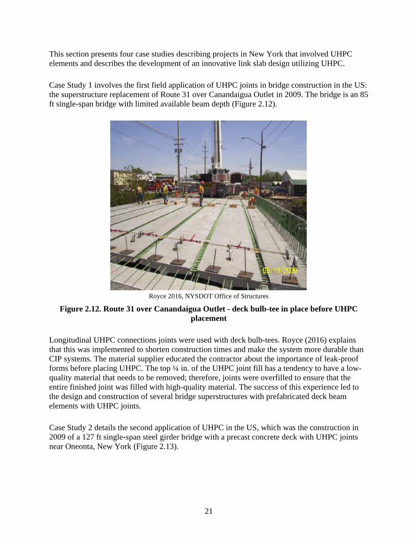
21
This section presents four case studies describing projects in New York that involved UHPC
elements and describes the development of an innovative link slab design utilizing UHPC.
Case Study 1 involves the first field application of UHPC joints in bridge construction in the US:
the superstructure replacement of Route 31 over Canandaigua Outlet in 2009. The bridge is an 85
ft single-span bridge with limited available beam depth (Figure 2.12).
Royce 2016, NYSDOT Office of Structures
Figure 2.12. Route 31 over Canandaigua Outlet - deck bulb-tee in place before UHPC
placement
Longitudinal UHPC connections joints were used with deck bulb-tees. Royce (2016) explains
that this was implemented to shorten construction times and make the system more durable than
CIP systems. The material supplier educated the contractor about the importance of leak-proof
forms before placing UHPC. The top ¼ in. of the UHPC joint fill has a tendency to have a low-
quality material that needs to be removed; therefore, joints were overfilled to ensure that the
entire finished joint was filled with high-quality material. The success of this experience led to
the design and construction of several bridge superstructures with prefabricated deck beam
elements with UHPC joints.
Case Study 2 details the second application of UHPC in the US, which was the construction in
2009 of a 127 ft single-span steel girder bridge with a precast concrete deck with UHPC joints
near Oneonta, New York (Figure 2.13).

22
Royce 2016, NYSDOT Office of Structures
Figure 2.13. Route 23 over Otego Creek in Oneonta - precast deck placement in progress
The UHPC placement operation was completed in two days without any major problems. Royce
(2016) says it could have been completed in a day if the contractor had sufficient labor and had
larger UHPC mixers. Careful storage of the UHPC premix through the storage period was
observed because any moisture penetration into the premix powder results in the formation of
silica balls in the UHPC mix (Royce 2016). To reduce or eliminate this problem, the supplier
improved the packaging and storage of the material as well as the mixing process. During the
placement of UHPC in the joints, a few areas of leakage were noticed and corrected during
construction. NYSDOT contract documents now alert contractors about the need for water-tight
forms (Royce 2016).
Case Studies 1 and 2 both utilized prefabricated components and achieved a considerable
reduction in construction time compared to conventional methods. After these projects were
completed, further improvements to this technology that would help accelerate construction were
identified. Among them were, first, to avoid the use of overlays over the precast components.
The use of concrete overlays was problematic due to the needed cure times, and avoiding their
use was a desirable improvement. As a solution, NYSDOT developed precast deck systems that
have a sacrificial thickness of ½ in. for diamond grinding after the completion of the deck to
obtain a smooth riding surface. Two types of composite connections were developed to avoid the
use of overlays: (1) UHPC haunches with open stud pockets in addition to the joints and (2)
hidden haunches with two types of fill material, cementitious grout or UHPC. The cementitious
grout fill material needed to have 6 in. studs penetrating above the bottom layer of the deck
reinforcement, while the UHPC-filled haunches were designed with 3 in. studs. The shorter studs
are allowable with the UHPC due to its high sustained tensile strength. The use of UHPC-filled
haunches with 3 in. studs was found to be the most efficient construction method, though the
material cost is bit higher. Second, accelerating the compressive strength gain of the UHPC
joints was identified as another desirable improvement. A compressive strength of 14 ksi was
determined to be adequate for the performance of UHPC joints under live traffic. To complete a

23
deck removal and replacement during one weekend closure, the available cure time for UHPC
was determined to be 12 to 14 hours.
Case Study 3 details the construction of two bridges on Route 42 over West Kill in Lexington,
New York. A 120 ft single-span precast deck over a new multi-girder steel superstructure with
UHPC joints over the steel girders is shown in Figure 2.14.
Royce 2016, NYSDOT Office of Structures
Figure 2.14. Route 42 over West Kill - panel joint placement in progress
These bridges were constructed during the winter of 2011 under an emergency contract. In
August of 2011, the original bridges were washed out during Hurricane Irene. Stud sheer
connectors were installed through openings in the deck panel with UHPC-filled haunches and
stud pockets. A diamond-ground deck surface with no overlay was used for these bridges. The
UHPC was cured under artificial heating because the ambient temperature during the curing time
was mostly below freezing. The NYSDOT is now confident that construction during wintertime
is feasible with the use of precast elements with UHPC. Even though UHPC joints need artificial
heating to cure, the heating setup is significantly less complex and the duration is shorter
compared to what would be needed for a CIP operation. In addition, based on the NYSDOT’s
past experience, artificial heating of CIP decks often results in deck cracking. That problem was
obviously avoided with these bridges (Royce 2016).
Case Study 4 involves many bridges constructed under various contracts in different parts of the
state. This group of bridges includes a number of single-span bridges, a two-span steel curve
girder bridge, and four three-span bridges. Ten of these bridges are located in urban areas
carrying Interstate traffic, while seven are on state highways in rural settings. The degree of
construction acceleration required was determined based on the needs of the specific location.
About half of these bridges required deck replacement within a window of 72 hours: from a
Friday night closure to an early Monday morning opening to traffic. Many of the bridges used 5

24
to 10 days of closure time. The cost of deck replacement increased with the degree of
acceleration. The NYSDOT allowed the longest window feasible to keep the cost as low as
possible. A typical example of one of these bridges can be observed in Figure 2.15.
Royce 2016, NYSDOT Office of Structures
Figure 2.15. I-81 over East Castle St. - precast deck placement in progress
This bridge is a 120 ft single-span precast deck without an overlay over an existing multi-girder
steel superstructure. Construction involved UHPC joints placed over the steel girders, hidden
haunches with non-shrink grout, and studs penetrating above the bottoms of the precast panels
(Royce 2016).
In addition to constructing the bridges described above in the four case studies, the NYSDOT
Office of Structures also developed an innovative link slab design utilizing UHPC to eliminate
transverse deck joints wherever feasible. The link slab design assumes that the UHPC section is
subject to bending. The link slab also acts as a semi-rigid link between spans, transferring
compressive, tensile, and shear stresses due to various loads (Royce 2016). The design of the link
slab is influenced by variables such as span arrangement, bearing type and arrangement, girder
end rotation due to live load, and bridge skew. A conceptual design of this link slab is shown in
Figure 2.16.

25
Royce 2016, NYSDOT Office of Structures
Figure 2.16. NYSDOT link slab cross-section
Several rehabilitation projects utilizing UHPC link slabs to eliminate joints are in progress at the
NYSDOT. Based on the NYSDOT’s experience as of 2016, the link slabs are performing well,
with no visible cracks within the UHPC slabs (Royce 2016). Figure 2.17 shows a finished link
slab.

26
Royce 2016, NYSDOT Office of Structures
Figure 2.17. Finished NYSDOT link slab
2.2.2.2 UHPC in Illinois
Liu and Schiff (2016) present the design and construction of Illinois’s first precast deck panel
bridge with UHPC joints, the $450 million Circle Interchange Project in Chicago. This project
involved the replacement of the Peoria Street Bridge over I-290 and a Chicago Transit Authority
(CTA) train station with a three-span continuous steel plate girder bridge with a total length of
273 ft 0 in. and a width of 56 ft 4 in. Three alternatives were proposed to the Illinois DOT
(IDOT) for consideration: (1) precast deck panels with internal post-tensioning, (2) an
AccelBridge system, and (3) precast deck panels with UHPC joints. IDOT decided to select the
new-generation deck system: precast deck panels with UHPC joints.
The bridge has 52 deck panels in total, and a longitudinal UHPC joint is provided to
accommodate the 56 ft wide bridge. Twenty different deck panels are required due to the
complex bridge layout, which accommodates a CTA train station entrance to the west, a CTA
staircase to the east, and light poles and drainage scuppers. All of the transverse and longitudinal
joints are filled with UHPC. The design of the UHPC joints is based on pull-out research. The
UHPC transverse joint and longitudinal joint details are shown in Figure 2.18 and Figure 2.19,
respectively.

27
Liu and Schiff 2016, IDOT
Figure 2.18. Circle Interchange Project - UHPC transverse joint
Liu and Schiff 2016, IDOT
Figure 2.19. Circle Interchange Project - UHPC longitudinal joint
The shear stud pockets are filled with non-shrink grout. The shear stud pocket detail is presented
in Figure 2.20. (Shear stud pockets utilizing UHPC are described below for the New Jersey
project.)

28
Liu and Schiff 2016, IDOT
Figure 2.20. Circle Interchange Project - shear stud pocket
Deck construction started in May 2015, and deck panel construction took about 10 days to
complete.
2.2.2.3 UHPC in New Jersey
McDonagh and Foden (2016) detail the benefits of using UHPC for the rehabilitation of the
Pulaski Skyway, a four-lane, 3.5-mile-long viaduct located in northern New Jersey that serves as
a direct link to New York City via the Holland Tunnel. Because of the critical nature of the
Skyway to the region’s transportation system and the narrowness of the structure, which makes it
difficult to perform maintenance without impacting traffic, the New Jersey DOT (NJDOT)
desired that the new bridge deck would have a service life of 75 years, with little maintenance
required during that time. Consequently, plant-cast concrete deck panels with stainless steel
reinforcing bars and field-cast UHPC panel closure joints were selected as the re-decking system.
UHPC is used in three specific situations on the Pulaski Skyway: for the transverse panel-to-
panel joints throughout the project, to fill the shear connections and haunches between the panels
and the steel framing, and to fill the longitudinal joint at the median of the bridge. Each of these
uses and their benefits are described below.
The majority of the transverse panel-to-panel joints on the project are 8 in. wide, as shown in
Figure 2.21.

29
New Jersey DOT, McDonagh and Foden 2016
Figure 2.21. Pulaski Skyway - typical transverse joint
The high strength of UHPC allows for the use of short reinforcing bars and lap splice lengths,
which enables the use of very narrow panel joints. This maximizes the amount of precast
concrete deck and minimizes the amount of CIP material, which results in time savings. The fast
cure time means that in as little as 24 hours after pouring the joints, the panels can be put into
service, either for construction or service loads. The high flowability of UHPC means that there
is a very low risk of unconsolidated material or air pockets in the joints. Finally, the deck panels
are more likely to crack and see reinforcing bar corrosion than the joints because of the high
durability and strength of the UHPC. This ensures that all of the durability measures
incorporated into the precast panels themselves will be fully realized and not compromised by
the panel joints.
A typical full-depth precast concrete panel used for the new Pulaski Skyway deck has
rectangular shear pockets to facilitate the connection between the panels and the shear studs so
that the panels will act compositely with the underlying steel framing. The panels are also
connected to the stringers and floor beams, although rather than using rectangular block-outs, the
entire length of the underlying stringers and floor beams is blocked out. The haunches are
beneath the panel between the pockets for the typical precast panel but integral with the
continuous block-outs for the panels.
These haunches and shear pockets were not originally designed to be UHPC, as can be seen in
Figure 2.22, which indicates two different grouts, Type A and Type B.

30
New Jersey DOT, McDonagh and Foden 2016
Figure 2.22. Pulaski Skyway - typical shear pocket detail
However, the contractor elected to use UHPC in order to combine the pockets with the haunches
as well as the pockets with the transverse joints into a single pour. The high strength of the
UHPC in the pockets gave the designers and contractor some added flexibility over shear stud
placement. Since minimum shear stud spacing criteria are typically based on local failure of the
concrete around the stud, the extremely high strength of the UHPC meant that the designers
could accept tighter spacing of the shear studs when conditions required it.
As with the transverse joints, the fast curing time of UHPC means that the panels can be put into
service in as little as 24 hours. The high flowability of UHPC is critical for the haunches, which
are as thin as 5/8 in. The high durability and low permeability of UHPC ensures that the shear
pockets and block-outs, such as those used for the transverse joints, will never become weak
points in the precast deck system (McDonagh and Foden 2016).
In order to maintain partial traffic during the re-decking operation, only half of the Skyway was
permitted to be closed at any time. Therefore, the presence of the existing southbound roadway
carrying two lanes of traffic was a restriction for construction of the new northbound deck, which
also had to be configured to carry two lanes of traffic when completed so that traffic on the
existing southbound deck could be routed to the northbound side. This arrangement meant that
very little open space was available between the existing southbound deck and the new
northbound deck for the extension of rebar necessary to make the two halves continuous in the
final condition. This open space was typically only 10 to 12 in. wide.
As a result, the high strength of UHPC was critical for this application. The designers detailed 6
in. long rebar hooks extending out of the edge of the northbound precast panels along the
median. This provided more than enough extension to ensure that these bars would be fully

31
developed in the UHPC median concrete. The subsequently placed southbound precast panels,
which had the advantage of a 3 ft typical open median, had straight rebar extending out of the
panels along the median with a typical 12 in. extension. Lastly, a set of straight reinforcing bars 2
ft 8 in. long were placed in the median, lapping the rebar extending from both the northbound
and southbound panels, as shown in Figure 2.23.
New Jersey DOT, McDonagh and Foden 2016
Figure 2.23. Pulaski Skyway - typical median detail
Thanks to the high strength of the UHPC, this rebar had fully developed lap splices to the rebar
extending from each panel, thereby ensuring that the rebar that extends transversely across the
bridge is continuous between both edges of the bridge and across the median.
Once again, with UHPC curing in as little as 24 hours, construction can proceed quickly, and the
median can be loaded rather rapidly. Furthermore, the fluidity of UHPC eliminates any concern
for air pockets or unconsolidated concrete that could be caused by the anchors for the metal
median barrier that are cast in the median. Finally, as with the transverse panel joints, this
continuous longitudinal panel joint is stronger and more durable than the panels it is connecting,
thereby ensuring the long-term durability of the entire deck system.
Overall, with UHPC employed for nearly all precast panel connections, the connections are no
longer the weak points that they traditionally have been, both in terms of strength and durability.
Instead, the connections are the strongest and most durable points of the deck system, stronger
and more durable than the precast deck panels with shop-cast concrete and corrosion-resistant
rebar. All of these features of the deck system are expected to eliminate the need for major deck
maintenance over the next 75 years (McDonagh and Foden 2016).
2.2.4 UHPC Summary
Several examples of UHPC joints have been presented in this report, and many more can be
found in the literature and in the field. The documentation for these completed projects shows
that the technology is working and has met the needs of users and owners on a number of
projects in demanding situations. Given these positive experiences, designers could consider the

32
use of UHPC at critical locations, such as concrete units in which joint hardware is embedded or
deck or approach slab components that are subjected to higher stresses due to soil settlement or
impact loads.
2.3 Modeling and Analysis of Bridges
The present research required various bridge components to be modeled and analyzed using FE
models. A review of the literature was conducted to provide the research team with the necessary
background to use FE modeling to analyze various bridge components.
2.3.1 Modeling of Bridge Components
Various modeling practices for concrete decks and steel girders were reviewed in the literature.
With this variety of information comes different ways of considering boundary conditions and
constraints between the concrete deck and steel girders. These factors have to be included in FE
models to properly analyze the structures.
Four papers in particular were compared in terms of their modeling practices. The similarities
and differences among the four papers are highlighted in the following discussion.
2.3.1.1 Concrete and Steel Elements
Biggs et al. (2000) detailed the development of FE models used to analyze the composite action
and global response of a reinforced concrete deck and steel girders. In these models, the concrete
deck elements were modeled as shell element S4R, a four-node, doubly curved, thin or thick
shell element with reduced integration, hourglass control, and finite membrane strains. The steel
girder elements were modeled as three-dimensional, first-order beam element B31OS, a two-
node, linear, open-section beam in space. Similarly, Klein (2006) developed separate FE models
for composite bridge deck bridges with reinforced concrete slabs and longitudinal steel girders.
The models were varied in terms of girder spacing to identify the optimum case from among the
responses obtained from the FE results. For both the concrete deck and the steel girders, shell
element S4R was utilized. The results stage of the modeling is shown in Figure 2.24.

33
Klein 2006
Figure 2.24. Full 3D finite element model
Bengtsson and Widén (2010) discussed the development of FE models to investigate fatigue
cracks observed in the Vårby Bridge near Stockholm, Sweden. The Vårby Bridge was modeled
with 3D deformable shell elements for all elements, including both the concrete deck and the
steel girders. The composite bridge model was built up from four different parts for the steel
details and one part representing the concrete deck. The deck was divided into a number of
different strips along the bridge to simulate the different thicknesses of the concrete deck
(Bengtsson and Widén 2010). The components of the model can be seen in Figure 2.25 and
Figure 2.26. A full view of the model can be seen in Figure 2.27.

34
Bengtsson and Widén 2010
Figure 2.25. Vårby Bridge 2010 - steel girders
Bengtsson and Widén 2010
Figure 2.26. Vårby Bridge 2010 - concrete deck

35
Bengtsson and Widén 2010
Figure 2.27. Vårby Bridge 2010 - full 3D FE model
A subsequent paper on the Vårby Bridge investigation undertook a numerical analysis and
updated the model. Abdulrahman and Portus (2015) developed FE models with a wide range of
parameter combinations. In these models, the concrete deck was modeled as shell elements while
beam elements were used in most of the steel girders and crossbeams. Shell elements were used
in the main girders. The main girders were identified as the girders that were monitored with
strain gages during previous phases of the investigation. The beam elements can be seen in
Figure 2.28, while the main girders can be seen in Figure 2.29.
Abdulrahman and Portus 2015
Figure 2.28. Vårby Bridge 2015 - beam elements

36
Abdulrahman and Portus 2015
Figure 2.29. Vårby Bridge 2015 - main girders
2.3.1.2 Boundary Conditions
Both Biggs et al. (2000) and Klein (2006) modeled the steel girders in their FE models as simply
supported structures. One end of the structure was pinned while the opposite end was a
pinned/sliding restraint. The nodes chosen for the boundary condition allocation were located at
each end of the bottom side of the girders. One end was restrained for the three displacement
directions, while the opposite end was restrained in only two directions. The nodes were not
supported in the longitudinal direction of the bridge. This condition resulted in a sliding behavior
for the simply supported condition being modeled (Klein 2006).
In the Vårby Bridge investigation, Bengtsson and Widén (2010) detailed the boundary conditions
for the two main girders. There were seven supports for the two main girders, C and D. The
bridge was free to move along the longitudinal axis (x-axis) for both girders, but only girder C
could move in the transverse direction (z-axis). This applied for all supports but the mid
supports, where the bearings were fixed for main girder D and partially fixed for main girder C
(Bengtsson and Widén 2010). The boundary conditions are summarized in Table 2.1.
Table 2.1. Vårby Bridge 2010 - boundary conditions
Bengtsson and Widén (2010)

37
Just like in Klein (2006), the boundary conditions in Bengtsson and Widén (2010) were attached
to one node located directly under the web in the main girders and in line with the vertical web
stiffeners. To represent the bearings in a reasonable way, the horizontal plates under the vertical
support stiffeners in the bottom flange were free to rotate around the node using a multi-point
constraint (MPC) (Bengtsson and Widén 2010). This is shown in Figure 2.30.
Bengtsson and Widén 2010
Figure 2.30. Vårby Bridge 2010 - boundary condition MPC
Abdulrahman and Portus (2015) detailed the boundary conditions in a subsequent paper on the
Vårby Bridge investigation. It is noteworthy that the boundary conditions from the Bengtsson
and Widén (2010) paper were kept intact. The boundary conditions depend mostly on the bearing
pads used in a particular bridge. Since the same bridge was under investigation in both studies,
the bearing pads remained constant and the boundary conditions therefore stayed the same.
2.3.1.3 Constraints
Different constraints between the concrete deck and steel girders were used across the four
papers discussed in this literature review. Even the two papers on the Vårby Bridge investigation
implemented different constraints. Shear studs are present in most, if not all, steel girder bridges.
These studs may elongate during uplift loads on the bridge deck since the shear studs are
embedded into the concrete. The studs would prevent the deck from lifting off the top flange of
the girders. Different ways of modeling this constraint are evident across the papers.
Biggs et al. (2000) modeled the constraints between the concrete deck and steel girders by
employing MPCs similar to the one shown in Figure 2.30. On the other hand, Klein (2006) used
tie constraints assuming full interaction between the two elements and transference of all degrees
of freedom.

38
Similarly to Klein (2006), Bengtsson and Widén (2010) also used tie constraints between the
concrete deck and the steel girders in the FE models developed for the Vårby Bridge
investigation. In a subsequent paper, Abdulrahman and Portus (2015) employed very different
constraints on multiple elements of the FE model. Since the main girders were modeled as a
combination of beam elements and shell elements, these different elements had to be connected
to model continuous beam behavior. MPCs were employed to connect the beam and shell
elements. MPCs were also used to connect the crossbeams to the main girders. Web stiffeners
were modeled in the main girders and were used as the source of the MPCs. Both applications of
MPCs can be seen in Figure 2.31 and Figure 2.32.
Abdulrahman and Portus 2015
Figure 2.31. Vårby Bridge 2015 - main girder constraints
Abdulrahman and Portus 2015
Figure 2.32. Vårby Bridge 2015 - crossbeam constraints
In Abdulrahman and Portus (2015), the interaction between the concrete deck and the steel
girders was modified from the previous paper on the Vårby Bridge investigation. In Bengtsson
and Widén (2010), these two elements were connected with a tie constraint between the bottom

39
surface of the concrete deck and the top face of the top flanges of the main steel girders. In
Abdulrahman and Portus (2015), the connection was modeled with linear axial springs. These
linear axial springs connected the main steel girder and the concrete deck. The springs were
modeled using two different approaches: engineering springs (SPRING2) and connectors
(CONN3D2); both approaches are illustrated in Figure 2.33.
Abdulrahman and Portus 2015
Figure 2.33. Vårby Bridge 2015 - deck and main girder constraints
Abdulrahman and Portus (2015) provide the following overview of both approaches:
When using the SPRING2 approach in Abaqus, the springs are modeled in such a way
that they are very stiff in the y and z directions so that the only action that is active is the
slip action between the steel and concrete, i.e., the stiffness of the spring in the x
direction.
The other approach is to use connector elements, CONN3D2, where wires are created
between the mesh-nodes of the bridge deck and the longitudinal beams. The wires are

40
then assigned different properties, having rigid connections in the y and z directions and a
defined stiffness in the x direction. (Abdulrahman and Portus 2015)
2.3.2 Modeling of Approach Slab and Soil Support
To further develop the deck over backwall concept, FE models of full-scale bridges had to be
modified to factor in the possible effects of the concept on the existing structures. The concept
includes an approach slab extending from the existing bridge deck on one end to the roadway
pavement on the other. To help model this feature, a review of the literature on approach slab
modeling was conducted.
Rajek (2010) used FE models to analyze the possible causes of approach slab deterioration. The
models included the bridge roadway, approach slab, abutment, and fill because all of these
elements relate to approach slab deterioration. Parametric studies were performed to determine
the influential parameters that contribute to the deterioration of the approach slab. Rajek (2010)
lists the parameters as void geometry, abutment height, approach slab length, soil stiffness,
concrete stiffness, and joint restrictions (i.e., for the joint between the roadway and approach
slab).
The approach slab incorporated in the model was made to conform to Wisconsin DOT
(WisDOT) standard specifications. WisDOT specifies a length of 15 ft 8 in. and a thickness of 1
ft for its standard approach slabs (Rajek 2010). The width of the approach slab was the minimum
lane width (12 ft) as defined by the 2007 American Association of State Highway and
Transportation Officials (AASHTO) specifications. Rajek (2010) explains that friction was the
primary constraint utilized in the model to control all concrete-to-concrete and soil-to-concrete
interactions. The coefficient of friction used to define all concrete-to-concrete interactions was
taken from section 11.6.4.3 of ACI 318-08.
Plane strain and plane stress elements were used in the model. Plane strain quadrilateral
quadratic elements with reduced integration were used for the soil region (Helwany 2007). Plane
stress quadrilateral quadratic elements with reduced integration were used for all concrete parts.
A section view of the model is shown in Figure 2.34 with all the pertinent elements labeled.
Rajek 2010
Figure 2.34. Section view of approach slab modeling

41
A vertical displacement restraint was implemented at the bottom of the soil to simulate very stiff
natural soils or bedrock at depth. Horizontal displacement restraints were placed at the sides of
the soil. The bottom of the abutment was fixed to simulate a rigid pile and pile connection (Rajek
2010). These can be seen in Figure 2.35.
Rajek 2010
Figure 2.35. Boundary conditions for approach slab modeling
The soil was modeled as a compacted sandy soil using the elastoplastic Mohr-Coulomb material
model within Abaqus. The sand emulated in the model was modeled after portage sand, as
discussed by Schuettpelz et al. (2010). The soil properties are shown in Table 2.2.
Table 2.2. Soil properties for approach slab modeling
Rajek 2010
The geometry of the settlement trench formed under the approach slab was varied in the
parametric study. The settlement trench geometries used in the parametric study are shown in
Figure 2.36. These are in general agreement with the observations of Cosgrove and Lehane
(2003).
Rajek 2010
Figure 2.36. Trench geometry for approach slab modeling
Rajek (2010) explains this approach to trench geometry as follows:

42
[W]hile standard practice dictates that the angle of the settlement trench be equal to the
constant volume friction angle (32.5°), the model utilized for this study set the angle of
the settlement trench at approximately 26.5°. This was assumed accurate as the saturation
of the soil and water pressure buildup within the soil would cause an increase in pore
pressures. The effective stress of the soil would decrease as a result of the increase in
pore pressure. (Rajek 2010)

43
CHAPTER 3. FINITE ELEMENT MODELING AND ANALYSIS
Two case study bridges were considered throughout the course of the research. The first bridge is
located on I-35 (Northbound, 049310; Southbound, 049320) 3.3 miles south of SR E-18 over
Bear Creek in Story County. The second bridge is located on IA-330/Marshalltown Blvd. 2.5
miles southwest of Melbourne over the North Skunk River in Marshall County. These bridges
will be referred to as the Story County bridge and the Marshall County bridge.
The selected bridges were analyzed using FE models that were developed to model the
conditions of the bridges presented in the original drawing plans. The information for the FE
analyses was obtained from as-built drawings, design documents, and expansion joint
specifications for the Story County bridge and the Marshall County bridge. For the analysis,
AASHTO specifications were followed to evaluate the behavior of the bridges.
The analysis results will eventually be used to identify critical conditions to guide the
development of a plan for post-construction testing of the structures and to correlate field
responses with the predictions from the models. Subsequently, the models may be calibrated
using the future field test results in order to increase the models’ accuracy. The verification of
the models will permit their confident use for designing expansion joints in the future.
3.1 Story County Bridge
A full 3D model was developed in Abaqus FEA for the Story County bridge. This model
includes a concrete bridge deck supported by welded plate steel girders and diaphragms that rest
on abutments at the ends and piers. A full 3D model can be seen in Figure 3.1, with a sectional
view in Figure 3.2.
Figure 3.1. Story County bridge - full 3D FE model

44
Figure 3.2. Story County bridge - section view
Constraints, boundary conditions, and other elements were assigned in the model. Loading
conditions due to self-weight, surface weathering, and truck loading were also incorporated into
the model.
An 8 in. by 338 ft bridge deck was modeled as a C3D8R element, which is an eight-node linear
brick element with reduced integration and hourglass control. In addition, C3D8R was utilized
for all concrete parts in the model, including the abutments and piers with their corresponding
column and beam dimensions. The steel superstructure is composed of welded plate steel girders
and transverse diaphragms at the ends and over the piers. The web and flanges of the welded
plate girders as well as the diaphragms were modeled as S4R elements, which are four-node,
doubly curved, thin or thick shell elements with reduced integration, hourglass control, and finite
membrane strains. For the flanges of the welded plate girders, width and thickness were modeled
per the drawing plans. All of the steel superstructure elements were merged together (Figure
3.3).
Figure 3.3. Story County bridge - steel superstructure
This model underwent an elastic analysis. Only mass density and elastic properties like Young’s
modulus and Poisson’s ratio were needed for a successful analysis. The mass densities utilized
for the concrete and steel were assigned as their specific weights: 150 lb/ft3 and 490 lb/ft3,
respectively. As for the Young’s modulus and Poisson’s ratio, 3,718 ksi and 0.15 was utilized for
the concrete and 29,000 ksi and 0.3 for the steel, respectively. In addition, the coefficients of

45
thermal expansion for both concrete and steel were selected as 5.5E-6 1/°F and 6.5E-6 1/°F,
respectively.
Boundary conditions were assigned to the abutment’s vertical and horizontal faces that are in the
direction of the supporting soil. Vertical faces have horizontal constraints and horizontal faces
have vertical constraints. A fixed boundary condition was assigned to the bottom face of the pier
columns, simulating the foundations that rest under the topsoil. Boundary conditions can be seen
in Figure 3.4 as red lines at the abutment and on the bottom face of the pier.
Figure 3.4. Story County bridge - boundary conditions
Tie constraints were assigned between the beams and columns of the piers. Tie constraints were
also assigned between the top flanges of all the welded plate girders and the bottom surface of
the bridge deck. Connection wires were utilized between the steel girders and the abutments and
piers to simulate the rocker and fixed bearings at their locations. All reaction values presented in
the following pages correspond to these connection wires.
3.1.1 Convergence Study
The model was trialed on numerous occasions with various meshing sizes. The results stabilized
at an approximate meshing size of 5 in. A meshing size of 4 in. was determined to be the most
effective for the model at this point. The time elapsed to complete the analysis for a meshing size
of 3 in. was almost five times as long as the time elapsed for a meshing size of 4 in. (Table 3.1).

46
Table 3.1. Story County bridge - mesh convergence study
Mesh Size (in.) Max Deflection at Midspan (in.) Time Elapsed (s)
8 1.242 108.4
6 1.248 178.6
5 1.035 416.1
4.5 1.031 552
4 1.032 785.2
3.5 1.031 1056.6
3 1.031 4641
The time elapsed for each trial is shown for all mesh sizes along with their deflection values.
A graph of the different values that were trialed with their results is shown in Figure 3.5.
Figure 3.5. Story County bridge - mesh convergence study
With a mesh size of 4 in., the structure was modeled using 332,627 elements, 437,973 nodes, and
1,663,341 variables.

47
3.1.2 Validation with Original Plans
The information needed to create the FE model and conduct the analysis for the Story County
bridge was obtained from its original drawing plans. The abutment and pier reactions can be
observed in these plans and in Table 3.2.
Table 3.2. Story County bridge - abutment and pier reactions from the drawing plans
Abutment Reactions (kips) Pier Reactions (kips)
Exterior Interior Exterior Interior
DL #1 31 47.1 113.4 172.1
DL #2 21.5 4.5 74.5 15.5
ULL - - 67 78
CLL - - 19.6 22.8
HS20-16 48.2 56.3 - -
Impact 10.6 12.3 17.9 20.8
Total 111.3 120.2 292.4 309.2
Source: Story County Bridge Plans
Dead load #1 includes weight of slab, girders, and diaphragms.
Dead Load #2 includes weight of curbs, rail, and future wearing surface.
These reactions were the source of comparison for the results obtained from the FE analysis
shown in the following section. It is important to mention that the FE model does not fully
incorporate all of the elements shown in the plans but includes the most pertinent ones.
Note that an HS20-16 truck load is shown in Table 3.2. References to this truck load were not
found in the literature. Therefore, this truck load was assumed to be an HS20-44 truck loading
condition and was allocated in the same manner as the other loads in the FE model. Even though
this truck load was assumed to be HS20-44, it is referred to as HS20-16 in the discussion.
3.1.2.1 Dead Load Reactions and Deflection
Self-weight was included in the whole model. A surface weathering loading condition of 19
lb/ft2 over the roadway was also added. Curb loading on 1.5 ft of the edges was added as a
surface area simulating a 2 ft 8 in. by 1 ft area of concrete along the entire length of the bridge
deck. The results for dead load deflection and a comparative loading conditions table are shown
in Figure 3.6, Figure 3.7, and Table 3.3.
Story County Bridge Plans
Figure 3.6. Story County bridge - anticipated dead load deflection

48
Figure 3.7. Story County bridge - deformation contour plot for dead load
Table 3.3. Story County bridge - dead load abutment and pier reactions
The maximum deflection obtained was approximately 1 in. at the center of the bridge. This value
correlates with the value obtained from the original drawing plans. The resulting abutment and
pier reactions were tabulated and compared with the values obtained from the drawing plans.
Two dead load loading conditions were considered for the pier and abutment reactions. Lower
percentages of difference were achieved for the exterior reactions than for the interior reactions,
mainly due to the oversimplification in the original drawings regarding the curb and railing load.
Both pier reactions show low percentages of difference from the total reaction, 2.45% for the
exterior support and 5.48% for the interior support. The abutment reactions also show low
percentages of difference from the total reaction, 2.69% and 0.22% for the exterior and interior
reactions, respectively.
3.1.2.2 Temperature Loading
Temperature loading was also modeled. The rocker and expansion plate settings from the
original drawing plans are shown in Table 3.4.
Ext % diff Int % diff Ext % diff Int % diff
DL #1 33.08 6.71 44.54 5.44 124.87 10.11 154.39 10.29
DL #2 18.01 16.24 6.95 54.47 58.43 21.57 22.94 48.00
Total 51.09 2.69 51.49 0.22 183.30 2.45 177.33 5.48
Pier Reactions (kips)Abutment Reactions (kips)

49
Table 3.4. Story County bridge - expansion plate settings
Story County Bridge Plans
A shrinkage and expansion of 0.5 in. can be seen at 10°F and 90°F, respectively, with a base
temperature of 50°F.
The results from the FE modeling for temperature can be seen in Figure 3.8.
Figure 3.8. Story County bridge - deformation contour plot for temperature loading
A maximum deformation of approximately 0.5 in. was obtained from the FE modeling. This
value matches the original plan value noted above. The results obtained from the FE modeling
were also compared to the values obtained using equation (1).
∆𝐿 = 𝛼∆𝑇𝐿 (1)
where ΔL is the change in length, α is the coefficient of thermal expansion of the material, ΔT is
the change in temperature, and L is the original length.
For the Story County bridge, the original length was taken as half of the total length of the bridge
deck, 169 ft or 2,028 in., resulting in a change in length of approximately 0.45 in. when the

50
change in temperature equals 40°F and the coefficient of thermal expansion of concrete is used,
5.5E-6 1/°F. The value obtained results in a percentage of difference of 10% from the original
plan value and the FE results.
3.1.2.3 Live Load Reactions and Deflection
HS20-44 truck loading conditions per AASHTO specifications were modeled and placed on top
of the bridge deck. Based on the AASHTO specifications, the wheel loads were assumed to be
uniformly distributed over an area of 20 in. by 10 in. The wheel spacing and loading is shown in
Figure 3.9.
Ghosn and Fiorillo 2013
Figure 3.9. HS20-44 loading conditions and tire spacing
A linear load of 0.640 kips per linear foot of lane over a 10 ft width was also included in the
truck loading conditions. This was modeled as a surface area over the length of the bridge. The
concentrated loads and linear load can be seen in Figure 3.10.
Original source unknown
Figure 3.10. HS20-44 loading conditions and uniform live load
Impact loads were also considered. A 20% impact load based on the concentrated load from the
tires was modeled. This impact load was calculated according to equation (2).

51
𝐼 = 50
𝐿+125 ≤ 0.3 (2)
where L is the longest span of the bridge in feet.
For the Story County bridge, the longest span is equal to 132 ft, which results in an impact load
of approximately 19.46%. Because of this result, a 20% impact load was used.
3.1.2.3.1 Controlling Truck Loading Conditions
A 3D model was created in VBridge. This program was used to verify the controlling truck
loading conditions to maximize the desired results (deflection, pier reactions, abutment
reactions). The 3D model can be seen in Figure 3.11.
Figure 3.11. Story County bridge - full 3D VBridge model
HS20-44 truck loading conditions per AASHTO specifications were modeled and placed on top
of the bridge deck. The controlling truck loading conditions for the abutment reactions, pier
reactions, and deflection can be seen in Figure 3.12, Figure 3.13, and Figure 3.14, respectively.

52
Figure 3.12. Story County bridge - controlling truck loading conditions for abutment
reactions
Figure 3.13. Story County bridge - controlling truck loading conditions for pier reactions

53
Figure 3.14. Story County bridge - controlling truck loading conditions for deflection
The lane load allocations can be seen in Figure 3.15, Figure 3.16, and Figure 3.17.
Figure 3.15. Controlling lane load for abutment reactions
Figure 3.16. Controlling lane load for pier reactions
Figure 3.17. Controlling lane load for deflection
3.1.2.3.2 Truck Loading Deflection
The Story County bridge model was loaded with the truck loading conditions discussed above.
The load allocation that corresponds with the maximum deflection at the midspan of the bridge

54
can be seen in Figure 3.14 for the truck load and Figure 3.17 for the lane load. The load in the
model can be seen in Figure 3.18.
Figure 3.18. Story County bridge - load allocation for deflection
Lane load is marked in red in the interior span. Two concurrent 10 ft wide pressure loads were
modeled in the center of the roadway. The truck load is shown with orange arrows indicating the
location and direction.
Two HS20-44 trucks were modeled acting over each lane load location. The results for these
loading conditions can be seen in Figure 3.19.
Figure 3.19. Story County bridge - deformation contour plot for deflection truck load

55
From the results of the FE model, a maximum deflection at midspan of approximately 2.5 in.
was obtained. AASHTO specifications provide certain deflection limits for vehicular bridges in
the absence of other criteria. These limits are set as L/800 for general vehicular loads and L/1000
for vehicular and pedestrian loads, where L is the span where the deflection is being questioned.
Since the Story County bridge does not have pedestrian loads, L/800 is applicable. Using the
center span of the Story County bridge, for which L is 132 ft or 1,584 in., the L/800 design limit
is approximately 1.98 in. Accounting for the dead load deflection shown previously, the live load
resulted in a deflection of approximately 1.53 in., which is lower than the L/800 deflection limit.
3.1.2.3.3 Truck Loading Reactions
To maximize the abutment and pier reactions, different truck loading allocations were needed.
The load allocation that corresponds with the maximum abutment reactions can be seen in Figure
3.12 for the truck load and Figure 3.15 for the lane load. The load allocation that corresponds
with the maximum pier reactions can be seen in Figure 3.13 for the truck load and Figure 3.16
for the lane load.
The abutment reactions results will be discussed first. The load in the model is shown in Figure
3.20 marked in red.
Figure 3.20. Story County bridge - load allocation for abutment reactions
The lane load can be clearly seen in the exterior spans with the rear axle of the concentrated
truck load at the edge of the bridge deck. Two HS20-44 trucks were modeled side by side, with
one side of the truck axle 2 ft from the curb. The lane loads were modeled as two concurrent 10
ft wide pressure loads starting from the curb.
A deformation contour plot is provided in Figure 3.21.
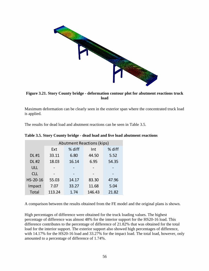
56
Figure 3.21. Story County bridge - deformation contour plot for abutment reactions truck
load
Maximum deformation can be clearly seen in the exterior span where the concentrated truck load
is applied.
The results for dead load and abutment reactions can be seen in Table 3.5.
Table 3.5. Story County bridge - dead load and live load abutment reactions
A comparison between the results obtained from the FE model and the original plans is shown.
High percentages of difference were obtained for the truck loading values. The highest
percentage of difference was almost 48% for the interior support for the HS20-16 load. This
difference contributes to the percentage of difference of 21.82% that was obtained for the total
load for the interior support. The exterior support also showed high percentages of difference,
with 14.17% for the HS20-16 load and 33.27% for the impact load. The total load, however, only
amounted to a percentage of difference of 1.74%.
Ext % diff Int % diff
DL #1 33.11 6.80 44.50 5.52
DL #2 18.03 16.14 6.95 54.35
ULL - - - -
CLL - - - -
HS-20-16 55.03 14.17 83.30 47.96
Impact 7.07 33.27 11.68 5.04
Total 113.24 1.74 146.43 21.82
Abutment Reactions (kips)

57
After careful inspection of the original plan values, it was decided that it was necessary to alter
the truck loading conditions in the FE model to try to improve its accuracy compared to the
original plan values. The truck loading conditions for the model needed to be altered because the
loads in the plans are calculated based on a one-dimensional bridge analysis.
From the literature (Ryan et al. 2012), it was discovered that a 26 kip load was used instead of
the current HS20-44 truck loading conditions for the drawing plan values. This loading condition
is shown in Figure 3.22.
MnDOT 2012
Figure 3.22. Truck loading conditions from the drawing plans
To obtain the drawing plan values, the 26 kip load is divided into the two axles of the truck and
multiplied by various factors. For the interior girders, the load is multiplied by the load
distribution factor (LDF) obtained using equation (3).
𝐿𝐷𝐹 = 𝑆
5.5 (3)
where LDF is the load distribution factor and S is the girder spacing in feet.
For the exterior girders, equation (4) is used with the factor calculated in equation (5).
𝑔 = 𝑒𝑔𝑖𝑛𝑡𝑒𝑟𝑖𝑜𝑟 (4)
𝑒 = 0.6 +𝑑𝑒
10 (5)

58
where g is the LDF for the exterior girders, ginterior is the LDF for the interior girders, e is a
conversion factor from interior girder to exterior girder, and de is the distance between the
exterior girders to the center of the curb in feet.
An additional factor for skewed bridges can also be added. This factor is relevant for the
Marshall County bridge and will be discussed in the following section.
In addition, judging by the magnitudes of the original plan values, it was determined that an
impact load was applied on the lane load in addition to the concentrated live load from the tire
loads. This is contrary to the current AASHTO specifications.
The truck loading conditions in the FE model were altered to attempt to match the drawing plan
values. One truck was modeled instead of two, with an impact load applied on the lane load as
well. This new load allocation can be seen in Figure 3.23, with one truck instead of two in one of
the exterior spans.
Figure 3.23. Story County bridge - updated load allocation for abutment reactions
The results for dead load and abutment reactions can be seen in Table 3.6.

59
Table 3.6. Story County bridge - dead load and updated live load abutment reactions
A comparison between the results obtained from the updated FE model and the original plans is
shown.
The percentages of difference decreased in the interior support after the truck loading conditions
were altered. The HS20-16 load, which had a percentage of difference of 47.96% under the
previous loading conditions, now resulted in a percentage of difference of 5.64%. The total load
on the interior support decreased from 146.43 kips to 115.24 kips. The percentage of difference
decreased from 21.82% to 4.12%. The total load decreased because the interior support is now
taking only one side of the axle from the truck. Previously, the interior support took the same
axle plus another axle.
The exterior support did not exhibit major differences from the previous loading conditions. The
HS20-16 load went from 55.03 kips to 53.34 kips, and the impact load went from 7.07 kips to
10.67 kips. The percentage of difference for the total load on the exterior support went from
1.74% to 3.50%. This small change in the exterior support may be due to the fact that the
exterior support was already taking the same axle of the truck nearest to the curb. The HS20-16
load decreased because there was no truck load in the adjoining lane.
The pier reactions will be discussed in the remainder of this section. The load in the model is
shown in Figure 3.24 marked in red.

60
Figure 3.24. Story County bridge - load allocation for pier reactions
The lane load can be clearly seen in the spans on either side of the loaded pier, with the rear axle
of the concentrated truck load located over the pier. Two HS20-44 trucks were modeled side by
side, with one side of the truck axle 2 ft from the curb. The lane loads were modeled as two
concurrent 10 ft wide pressure loads starting from the curb.
A deformation contour plot is provided in Figure 3.25.
Figure 3.25. Story County bridge - deformation contour plot for pier reactions truck load
The maximum deformation is not prominent because much of the load is applied over a support.
The results for dead load and pier reactions can be seen in Table 3.7.

61
Table 3.7. Story County bridge - dead load and live load pier reactions
A comparison between the results obtained from the FE model and the original plans is shown.
High percentages of difference were obtained for the truck loading values. The highest
percentage of difference was almost 183.09% for the interior support for the concentrated live
load. This difference contributes to the percentage of difference of 4.03% that was obtained for
the total load for the interior support. The exterior support also showed high percentages of
difference, with 104.36% for the concentrated live load and 55.25% for the impact load. The
total load, however, only amounted to a percentage of difference of 0.38%.
For the reasons explained above for the abutment reactions, the truck loading conditions in the
FE model were altered to attempt to match the drawing plan values. One truck was modeled
instead of two, with an impact load applied on the lane load as well. This new load allocation can
be seen in Figure 3.26, with one truck instead of two in one of the exterior spans.
Figure 3.26. Story County bridge - updated load allocation for pier reactions
Ext % diff Int % diff
DL #1 126.23 11.31 150.29 12.68
DL #2 58.95 20.88 22.40 44.48
ULL 58.05 13.36 71.52 8.31
CLL 40.05 104.36 64.55 183.09
HS-20-16 - - - -
Impact 8.01 55.25 12.91 37.94
Total 291.29 0.38 321.66 4.03
Pier Reactions (kips)

62
The results for dead load and pier reactions can be seen in Table 3.8.
Table 3.8. Story County bridge - dead load and updated live load pier reactions
A comparison between the results obtained from the updated FE model and the original plans is
shown.
The percentages of difference decreased in the interior support after the truck loading conditions
were altered. The concentrated live load, which had a percentage of difference of 183.09% under
the previous loading conditions, now resulted in a percentage of difference of 42.60%. The
percentage of difference for the impact load decreased from 37.94% to 0.03%. The total load on
the interior support decreased from 321.66 kips to 297.51 kips. The percentage of difference
decreased from 4.03% to 3.78%. The total load decreased because the interior support is now
taking only one side of the axle from the truck. Previously, the interior support took the same
axle plus another axle.
The exterior support did not exhibit major differences from the previous loading conditions. The
concentrated live load went from 40.05 kips to 37.03 kips, and the impact load went from 8.01
kips to 19.02 kips. The percentage of difference for the total load on the exterior support went
from 0.38% to 2.35%. This small change in the exterior support may be due to the fact that the
exterior support was already taking the same axle of the truck nearest to the curb. The
concentrated live load decreased because there was no truck load in the adjoining lane.
3.2 Marshall County Bridge
A full 3D model was developed in Abaqus FEA for the Marshal County bridge. This model
includes a concrete bridge deck supported by welded plate steel girders and diaphragms that rest
on abutments at the ends and piers. A skew of 45° is also modeled. A full 3D model can be seen
in Figure 3.27, with a plan view in Figure 3.28, in which the skew is noticeable.
Ext % diff Int % diff
DL #1 126.24 11.32 150.29 12.68
DL #2 58.95 20.88 22.40 44.48
ULL 58.05 13.35 71.51 8.32
CLL 37.03 88.91 32.51 42.60
HS-20-16 - - - -
Impact 19.02 6.24 20.81 0.03
Total 299.28 2.35 297.51 3.78
Pier Reactions (kips)

63
Figure 3.27. Marshall County bridge - gull 3D FE model
Figure 3.28. Marshall County bridge - plan view
Constraints, boundary conditions, and other elements were assigned in the model. Loading
conditions due to self-weight, surface weathering, and truck loading were also incorporated into
the model.
An 8 in. by 210 ft bridge deck was modeled as a C3D8R element, which is an eight-node linear
brick element with reduced integration and hourglass control. In addition, C3D8R was utilized
for all concrete parts in the model, including the abutments and the pier caps. The steel
superstructure was composed of welded plate steel girders and transverse diaphragms at the ends
and over the piers. The web and flanges of the welded plate girders as well as the diaphragms
were modeled as S4R elements, which are four-node, doubly curved, thin or thick shell elements
with reduced integration, hourglass control, and finite membrane strains. For the flanges of the
welded plate girders, width and thickness were modeled per the drawing plans. All of the steel
superstructure elements were merged together (Figure 3.29).

64
Figure 3.29. Marshall County bridge - steel superstructure
This model underwent an elastic analysis. Only mass density and elastic properties such as
Young’s modulus and Poisson’s ratio were needed to execute the analysis successfully. The mass
densities utilized for the concrete and steel were assigned as their specific weights: 150 lb/ft3 and
490 lb/ft3, respectively. As for the Young’s modulus and Poisson’s ratio, 3,718 ksi and 0.15 were
utilized for concrete and 29,000 ksi and 0.3 were utilized for the steel, respectively. In addition,
the coefficients of thermal expansion for both concrete and steel were selected as 5.5E-6 1/°F
and 6.5E-6 1/°F, respectively.
Boundary conditions were assigned to the abutment’s vertical and horizontal faces that are in the
direction of the supporting soil. Vertical faces have horizontal constraints and horizontal faces
have vertical constraints. A fixed boundary condition was assigned to the bottom face of the pier
caps simulating the foundations that rest under the topsoil. Boundary conditions can be seen in
Figure 3.30 as red lines at the abutment and on the bottom face of the pier cap.
Figure 3.30. Marshall County bridge - boundary conditions

65
Tie constraints were assigned between the top flanges of all the welded plate girders with the
bottom surface of the bridge deck. Connection wires were utilized between the steel girders and
the abutments and piers to simulate the rocker bearings at their locations. All reaction values
presented in the following pages correspond to these connection wires.
3.2.1 Convergence Study
The model was trialed on numerous occasions with various meshing sizes. The results stabilized
at an approximate meshing size of 5 in. A meshing of 4 in. was determined to be the most
effective for the model at this point. Just for reference, the time elapsed to complete the analysis
for a meshing size of 3 in. was almost six times as long as the time elapsed for a meshing size of
4 in. (Table 3.9).
Table 3.9. Marshall County bridge - mesh convergence study
Mesh Size (in.) Max Deflection at Midspan (in.) Time Elapsed (s)
12 0.7187 77.7
10 0.7103 100.9
8 0.7513 144.5
6 0.7381 243.7
5 0.5261 654.7
4.5 0.5247 835
4 0.5272 1125.9
3.5 0.5375 1777.9
3 0.5213 11924.8
The time elapsed for each trial is shown for all mesh sizes along with their deflection values.
A graph of the different values that were trialed with their results is shown in Figure 3.31.

66
Figure 3.31. Marshall County bridge - mesh convergence study
With a mesh size of 4 in., the structure was modeled using 318,380 elements, 450,396 nodes, and
1,562,961 variables.
3.2.2 Validation with Original Plans
The information needed to develop the FE model and analysis for the Marshall County bridge
was obtained from its original drawing plans. Abutment and pier reactions can be observed in
these plans and in Table 3.10.
Table 3.10. Marshall County bridge - abutment and pier reactions from the drawing plans
Abutment Reactions (kips) Pier Reactions (kips)
Exterior Interior Exterior Interior
DL #1 24.5 27.8 90.1 102.0
DL #2 10.0 4.7 34.6 16.3
ULL - - 42.5 50.3
CLL - - 20.0 23.7
HS20-44 45.6 53.9 - -
Impact 12.0 14.2 15.8 18.7
Total 92.1 100.6 203.0 211.0
Source: Marshall County Bridge Plans
Dead load #1 includes weight of slab, girders, and diaphragms.
Dead Load #2 includes weight of curbs, rail, and future wearing surface.

67
These reactions were the source of comparison for the results obtained from the FE analysis
shown in the following section. It is important to mention that the FE model does not fully
incorporate all of the elements shown in the plans but includes the most pertinent ones.
3.2.2.1 Dead Load Reactions and Deflection
Self-weight was included in the whole model. A surface weathering loading condition of 20
lb/ft2 over the roadway was also added. Curb loading on 1 ft 8 in. of the edges was added as a
surface area simulating a 1 ft 8 in. by 1 ft area of concrete along the entire length of the bridge
deck. The results for dead load deflection and a comparative loading conditions table can be seen
in Figure 3.32, Figure 3.33, and Table 3.11.
Marshall County Bridge Plans
Figure 3.32. Marshall County bridge - anticipated dead load deflection
Figure 3.33. Marshall County bridge - deformation contour plot for dead load
Table 3.11. Marshall County bridge - dead load abutment and pier reactions
Ext % diff Int % diff Ext % diff Int % diff
DL #1 25.01 2.07 28.13 1.19 86.36 4.15 100.35 1.61
DL #2 10.17 1.67 4.75 1.10 33.99 1.76 16.68 2.35
Pier Reactions (kips)Abutment Reactions (kips)

68
The maximum deflection obtained was approximately 0.53 in. at the center of the bridge. This
value presents a percentage of difference of approximately 15% from the value obtained from the
original drawing plans (5/8 in.).
The resulting abutment and pier reactions were tabulated and compared with the values obtained
from the drawing plans. Two dead load loading conditions were considered for the pier and
abutment reactions. Both the pier and abutment reactions show low percentages of difference
ranging from a maximum of 4.15% to a minimum of 1.10%.
3.2.2.2 Temperature Loading
Temperature loading was also modeled. Expansion plate settings from the original drawing plans
are shown in Table 3.12.
Table 3.12. Marshall County bridge - expansion plate settings
Marshall County Bridge Plans
A shrinkage and expansion of 0.25 in. can be seen at 10°F and 90°F, respectively, with a base
temperature of 50°F.
The results from the FE modeling can be seen in Figure 3.34.

69
Figure 3.34. Marshall County bridge - deformation contour plot for temperature loading
A maximum deformation of approximately 0.3 in. was obtained from the FE modeling. This
value is 20% different than the original plan value. The result obtained from the FE modeling
was also compared to the value obtained using equation (1).
For the Marshall County bridge, the original length was taken as half of the total length of the
bridge deck, 105 ft or 1,260 in., resulting in a change in length of approximately 0.28 in. when
the change of temperature was 40°F and the coefficient of thermal expansion of concrete was
used, 5.5E-6 1/°F. The value obtained results in a percentage of difference of 6.22% from the
result obtained from the FE modeling.
3.2.2.3 Live Load Reactions and Deflection
The same loading conditions described in Section 3.1.2.3, Figure 3.9 and Figure 3.10, were
applied. Impact loads were also considered. A 25% impact load based on the concentrated load
from the tires was modeled. This impact load was calculated according to equation (2). For the
Marshall County bridge, the longest span is equal to 82 ft, which results in an impact load of
approximately 24.15%. Because of this result, a 25% impact load was used.
3.2.2.3.1 Controlling Truck Loading Conditions
A 3D model was created in VBridge. This program was used to verify the controlling truck
loading conditions to maximize the desired results (deflection, pier reaction, abutment reaction).
The 3D model can be seen in Figure 3.35, with a top view in Figure 3.36.

70
Figure 3.35. Marshall County bridge - full 3D VBridge model
Figure 3.36. Marshall County bridge - plan view of VBridge model
HS20-44 truck loading conditions per AASHTO specifications were modeled and placed on top
of the bridge deck.
The controlling truck loading conditions for the abutment reactions, pier reactions, and deflection
can be seen in Figure 3.37, Figure 3.38, and Figure 3.39, respectively.

71
Figure 3.37. Marshall County bridge - controlling truck loading conditions for abutment
reactions
Figure 3.38. Marshall County bridge - controlling truck loading conditions for pier
reactions

72
Figure 3.39. Marshall County bridge - controlling truck loading conditions for deflection
The controlling lane loads are the same as those shown in Section 3.1.2.3.1, Figure 3.16, Figure
3.17, and Figure 3.18. These conditions can be summarized as the lane load being applied on the
exterior spans to maximize abutment reactions, on the continuous spans to observe the reactions
of the piers in between, and on the center span to observe deflection at midspan.
3.2.2.3.2 Truck Loading Deflection
The Marshall County bridge model was loaded with the truck loading conditions discussed
above. The load allocation that corresponds with the maximum deflection at the midspan of the
bridge can be seen in Figure 3.39 for the truck load and Figure 3.17 for the lane load. The load in
the model can be seen in Figure 3.40.

73
Figure 3.40. Marshall County bridge - load allocation for deflection
Lane load is marked in red in the interior span. Two concurrent 10 ft wide pressure loads were
modeled in the center of the roadway. The truck load is shown with orange arrows indicating the
location and direction.
Two HS20-44 trucks were modeled acting over each lane load location. The deflection results
for these loading conditions can be seen in Figure 3.41.
Figure 3.41. Marshall County bridge - deformation contour plot for deflection truck load
From the results of the FE model, a maximum deflection at midspan of approximately 1.3 in.
was obtained. AASHTO specifications provide certain deflection limits for vehicular bridges in
the absence of other criteria. These limits are set as L/800 for general vehicular loads and L/1000
for vehicular and pedestrian loads, where L is the span where the deflection is being questioned.
Since the Marshall County bridge does not have pedestrian loads, L/800 is applicable. Using the
center span of the Marshall County bridge, for which L is 82 ft or 984 in., the L/800 design limit
is approximately 1.23 in. Accounting for the dead load deflection shown previously, the live load
resulted in a deflection of approximately 0.89 in. which is lower than the L/800 deflection limit.

74
3.2.2.3.3 Truck Loading Reactions
To maximize abutment and pier reactions, different truck loading allocation were needed. The
load allocation that corresponds with the maximum abutment reactions can be seen in Figure
3.37 for the truck load and Figure 3.15 for the lane load. The load allocation that corresponds
with the maximum pier reactions can be seen in Figure 3.38 for the truck load and Figure 3.16
for the lane load.
The abutment reactions results will be discussed first. The load in the model is shown in Figure
3.42 marked in red.
Figure 3.42. Marshall County bridge - load allocation for abutment reactions
The lane load can be clearly seen in the exterior spans with the rear axle of the concentrated
truck load at the edge of the bridge deck. Two HS20-44 trucks were modeled side by side, with
one side of the truck axle 2 ft from the curb. The lane loads were modeled as two concurrent 10
ft wide pressure loads starting from the curb.
A deformation contour plot is provided in Figure 3.43.

75
Figure 3.43. Marshall County bridge - deformation contour plot for abutment reactions
truck load
Maximum deformation can be clearly seen in the exterior span where the concentrated truck load
is applied.
The results for dead load and abutment reactions can be seen in Table 3.13.
Table 3.13. Marshall County bridge - dead load and live load abutment reactions
A comparison between the results obtained from the FE model and the original plans is shown.
High percentages of difference were obtained for the truck loading values. The highest
percentages of difference were 32.32% for the exterior support for the impact load and 27.07%
for the interior support for the HS20-44 load. These differences contribute to the percentages of
difference of 5.52% and 13.28% obtained for the total load for the exterior and interior support,
respectively.
For the same reasons explained under the discussion of the Story County bridge analysis, truck
loading conditions were altered to attempt to match the drawing plan values. One truck was
Ext % diff Int % diff
DL #1 24.10 1.65 27.90 0.36
DL #2 10.30 3.00 4.60 2.23
ULL - - - -
CLL - - - -
HS-20-44 44.50 2.41 68.49 27.07
Impact 8.12 32.32 12.98 8.62
Total 87.02 5.52 113.96 13.28
Abutment Reactions (kips)

76
modeled instead of two, with an impact load applied on the lane load as well. This new load
allocation can be seen in Figure 3.44, with only one truck instead of two in one of the exterior
spans.
Figure 3.44. Marshall County bridge - updated load allocation for abutment reactions
The results for dead load and abutment reactions can be seen in Table 3.14.
Table 3.14. Marshall County bridge - dead load and updated live load abutment reactions
A comparison between the results obtained from the updated FE model and the original plans is
shown.
After the truck loading conditions were altered, the percentages of difference remained almost
constant for the total abutment reaction of both the interior and exterior supports. The total load
on the interior support decreased from 113.96 kips to 86.93 kips, yet the percentage of difference
increased from 13.28 % to 13.59%. Under the previous loading conditions, the load was 13.28%
higher than that of the original plan values, while under the altered truck loading conditions the
load was 13.59% lower. The total load of the exterior support remained almost constant as well:
Ext % diff Int % diff
DL #1 24.10 1.65 27.90 0.36
DL #2 10.30 3.01 4.60 2.22
ULL - - - -
CLL - - - -
HS-20-44 42.33 7.17 43.54 19.21
Impact 10.58 11.81 10.89 23.34
Total 87.31 5.20 86.93 13.59
Abutment Reactions (kips)

77
87.02 kips in the previous model and 87.31 kips in the altered truck loading model. The
percentage of difference decreased from 5.52% to 5.20%.
The pier reactions will be discussed in the remainder of this section. The load in the model is
shown in Figure 3.45 marked in red.
Figure 3.45. Marshall County bridge - load allocation for pier reactions
The lane load can be clearly seen in an exterior and middle span, with the rear axle of the
concentrated truck load loaded over the pier. Two HS20-44 trucks were modeled side by side,
with the one side of the truck axle 2 ft from the curb. The lane loads were modeled as two
concurrent 10 ft wide pressure loads starting from the curb.
A deformation contour plot is provided in Figure 3.46.
Figure 3.46. Marshall County bridge - deformation contour plot for pier reactions truck
load
Maximum deformation is not prominent because much of the load is applied over a support.
The results for dead load and pier reactions can be seen in Table 3.15.

78
Table 3.15. Marshall County bridge - dead load and live load pier reactions
A comparison between the results obtained from the FE model and the original plans is shown.
High percentages of difference were obtained for the truck loading values. The highest
percentage of difference was 221.37% for the interior support for the concentrated live load. This
difference contributes to the percentage of difference of 24.52% obtained for the total load for
the interior support. The exterior support also showed high percentages of difference, with
116.64% for the concentrated live load and 31.45% for the impact load. The total load, however,
only amounted to a percentage of difference of 5.56%.
For the reasons explained above for the abutment reactions, the truck loading conditions in the
FE model were altered to attempt to match the drawing plan values. One truck was modeled
instead of two, with an impact load applied on the lane load as well. This new load allocation can
be seen in Figure 3.47, with one truck instead of two in one of the exterior spans.
Figure 3.47. Marshall County bridge - updated load allocation for pier reactions
The results for dead load and pier reactions can be seen in Table 3.16.
Ext % diff Int % diff
DL #1 86.96 3.48 101.42 0.56
DL #2 33.96 1.85 16.65 2.17
ULL 39.20 7.77 49.46 1.67
CLL 43.33 116.64 76.17 221.37
HS-20-44 - - - -
Impact 10.83 31.45 19.04 1.82
Total 214.28 5.56 262.74 24.52
Pier Reactions (kips)

79
Table 3.16. Marshall County bridge - Dead load and updated live load pier reactions
A comparison between the results obtained from the updated FE model and the original plans is
shown.
The percentages of difference decreased in the interior support after the truck loading conditions
were altered. The concentrated live load, which had a percentage of difference of 221.37% under
the previous loading conditions, now resulted in a percentage of difference of 31.57%. The total
load on the interior support decreased from 262.74 kips to 218.54 kips. The percentage of
difference decreased from 24.52% to 3.57%. The total load decreased because the interior
support is now taking only one side of the axle from the truck. Previously, the interior support
took the same axle plus another axle.
The exterior support did not exhibit major differences from the previous loading conditions. The
concentrated live load decreased from 43.33 kips to 42.68 kips, and the impact load increased
from 10.83 kips to 20.48 kips. The percentage of difference for the total load on the exterior
support actually increased from 5.56% to 10.06%. Less change would be expected for the
exterior support because the exterior support was already taking the load of the same axle of the
truck nearest to the curb.
3.2.3 Joint and Approach Slab Modeling
The Marshall County bridge model was updated with the deck over backwall concept described
in Chapter 2. A 20 ft section was taken from the farthest abutment end in the longitudinal
direction. Since the bridge is skewed 45°, the other end would span a total of 64 ft. The bridge
deck was extended over the abutment interface while the top of the abutment was cut off.
Soil support was added as a C3D8R element, an eight-node linear brick element with reduced
integration and hourglass control. Three soil support compositions were taken into consideration:
loose, moderately stiff, and stiff. Soil properties for each one are shown in Chapter 2, Table 2.2.
Pertinent results are shown for all three compositions in the following pages. A 12 ft void was
modeled to be present in the direction away from the abutment backwall according to practices
Ext % diff Int % diff
DL #1 87.04 3.39 101.22 0.76
DL #2 33.98 1.79 16.62 1.95
ULL 39.24 7.68 49.38 1.83
CLL 42.68 113.39 31.18 31.57
HS-20-44 - - - -
Impact 20.48 29.61 20.14 7.70
Total 223.41 10.06 218.54 3.57
Pier Reactions (kips)

80
suggested by the Iowa DOT Office of Bridges and Structures (2018a). A 2:1 slope was used for
the horizontal to vertical distance of this void, as shown in Chapter 2, Figure 2.36.
A full-scale view of this model can be seen in Figure 3.48.
Figure 3.48. Full 3D FE model with approach slab
A section view of the abutment interface can be seen in Figure 3.49 and Figure 3.50.
Figure 3.49. Section view without end span beam

81
Figure 3.50. Section view with end span beam
In early developments of the detailing shown in Chapter 2, options included an end span beam
that encased the diaphragms. While the Marshall County bridge does not have this end span
beam, the effect of it on the various points of interest across the joint and approach slab can be
demonstrated by its inclusion.
The webs of the girders were embedded into the curb and end span beam. The top flanges of the
girders were also embedded into the curb. The end diaphragms were embedded into the end span
beam. The tie constraints between the top flanges of all of the welded plate girders and the
bottom face of the bridge deck were retained from the previous model. The top flanges of the end
diaphragms were constrained with the bottom face of the curb. Tie constraints were also used
between the bottom face of the bridge deck and the top face of the curb and between the bottom
face of the curb and the top face of the end span beam.
Boundary conditions remained identical to those of the model detailed previously for the
abutment and piers. New boundary conditions were assigned to the approach slab and soil. A
vertical constraint was assigned at the far edge of the approach slab. Horizontal constraints were
assigned to the vertical faces of the soil mass. Vertical constraints were assigned to the bottom
face of the soil mass. An additional constraint in a third direction was assigned to the skewed
face of the soil mass. These boundary conditions are shown in Figure 3.51 and Figure 3.52
marked in red.

82
Figure 3.51. Boundary conditions section view
Figure 3.52. Boundary conditions 3D view
A contact interaction was provided between the bottom face of the bridge deck (approach slab)
and the top face of the soil mass. This interaction is shown in Figure 3.53.

83
Figure 3.53. Contact interaction
In addition, connection wires were kept between the steel girders and the abutments/piers. All
reaction values presented in the following pages correspond to these connection wires.
With this model, the impact of the deck over backwall concept on the existing structure can be
predicted. Certain points of interest were identified as locations where the results of the model
would be reported. First and foremost, the increase in bearing loads due to the new dead load of
the bridge deck and support slab would be considered. Additional load would also be taken by
the bearings due to live loads on the approach slab, which was previously not considered.
Abutment reactions from the connection wires would be reported under various dead load and
live load conditions in order to provide an analysis of the bearing loads. Additionally,
deformation due to temperature loading, with the additional 20 ft of approach slab on one side
and 64 ft on the other side, would also be considered. Deflection values at the abutment interface
and at the midspan of the approach slab would also be reported. As reported here, midspan does
not refer to exactly the midspan of the approach slab, but mainly the region between the
abutment interface and the approach slab end support. Stress levels at the abutment interface and
the midspan were also identified as points of interest. Both the top and bottom faces of the bridge
deck (including the approach slab) would be considered.
The dead load reaction results from the FE model will be discussed first. Table 3.17 shows
abutment reactions in kips for the two dead loads.

84
Table 3.17. Dead load abutment reactions (kips)
The first two columns, corresponding to the dead loads with no end span beam, show the original
dead loads that are being transferred to the bearings on each support. The columns show the
values for DL#1 and DL#2 obtained previously. The remaining columns show the increase in
dead load for each specific element. For example, when the bridge was modeled with the end
span beam, 3.53 kips, 6.06 kips, 5.93 kips, 6.33 kips, and 3.33 kips were added to the DL#1
abutment reactions for the first exterior, first interior, second interior, third interior, and second
exterior supports, respectively. Notice that only DL#1 is shown for the column with the end span
beam section because adding this element does not affect DL#2. However, DL#2 is shown in all
other columns because a larger area for the future wearing surface is provided by the top face of
the approach slab.
When the approach slab was modeled with no soil support, the reactions showed the largest
increase in dead load, which was expected since the bearings are taking most of the self-weight
of the approach slab with only an edge support at the other end. The largest increase was seen at
the middle interior support, with 48.51 kips and 9.69 kips for DL#1 and DL#2, respectively. As
expected, when the soil support was modeled, these values decreased considerably. With each
increase in the soil stiffness, the load taken by the bearings decreased, although the difference is
minimal in some cases between a moderately stiff and a stiff soil. This relationship between the
moderately stiff and stiff soil is consistent throughout the results presented in the following
pages. This suggests that the truck load might not be large enough to deflect the slab and
compress a moderately stiff or stiff soil to the degree that it would affect the support that the soil
provides for the approach slab.
From top to bottom in Table 3.17, the first exterior reaction refers to the reaction closest to the 20
ft long section of the approach slab. Each subsequent reaction follows in the transverse direction
until the remaining exterior reaction, which corresponds to the 64 ft long section of the approach
slab.
Reactions for all possible combinations of dead load scenarios can be seen in Figure 3.54.
DL#1 DL#2 DL#1 DL#1 DL#2 DL#1 DL#2 DL#1 DL#2 DL#1 DL#2
Exterior 26.03 11.09 3.53 10.15 1.17 10.51 0.69 5.72 0.41 5.19 0.38
Interior 30.73 5.00 6.06 40.59 7.88 19.65 2.68 14.89 2.42 14.40 2.37
Interior 31.16 5.32 5.93 48.51 9.69 18.22 2.57 13.26 2.31 12.73 2.27
Interior 30.83 5.17 6.33 37.07 7.46 18.20 2.61 12.76 2.18 12.11 2.13
Exterior 27.82 10.70 3.33 7.53 1.04 8.30 1.13 7.80 1.06 7.71 1.06
SupportNo Beam Beam
Approach Slab
No SoilSoil
Moderately StiffLoose Stiff

85
Figure 3.54. Dead load abutment reactions
The figure shows that most combinations would fall in a range of approximately 40 to 60 kips.
Most of the lower values would correspond to exterior reactions while the higher values would
correspond to interior reactions. The highest values, over 80 kips, correspond to scenarios with
no support soil. The realistic values would fall within the 40- to 60-kip range mentioned above.
Two steps can be seen in the horizontal axis, where each step corresponds to a different loading
case. The first step corresponds to the combinations of DL#1, and the second step corresponds to
the additional load from the combinations of DL#2.
Temperature loading was also included in this FE model. The results from the previous FE
model can be seen in Figure 3.34. A maximum deformation of approximately 0.3 in. was
obtained from that model. The results for the model with the approach slab are shown in Figure
3.55; a maximum deformation of approximately 0.46 in. was obtained.

86
Figure 3.55. Deformation contour plot for temperature loading
This represents an increment of approximately 0.16 in. Comparing this value of 0.16 in. to the
value obtained from equation (1), approximately 0.17 in., the FE result closely matches the one
obtained from the equation. A percentage of difference of approximately 4% from the exact
value is obtained using the result from the equation as the base value.
To study the additional bearing loads due to live loads in the approach slab, various live load
configurations were modeled acting on the top face of the approach slab. Various live load
configurations were modeled as various truck loading allocations. The different truck cases are
detailed in Chapter 6, Figure 6.5, Figure 6.6, Figure 6.7, and Figure 6.8. In total, four cases were
considered. Figure 3.56, Figure 3.57, Figure 3.58, and Figure 3.59 show the truck load
allocations in the FE model for Case 1, Case 2, Case 3, and Case 4, respectively.
Figure 3.56. Case 1 - truck load allocation

87
Figure 3.57. Case 2 - truck load allocation
Figure 3.58. Case 3 - truck load allocation
Figure 3.59. Case 4 - truck load allocation

88
The truck load allocations are marked in red in the four figures. Truck loading conditions were
modeled as they were in Section 3.1.2.3, Figure 3.9 and Figure 3.10. Only the concentrated live
load from the tires was considered in this investigation. However, the impact values can be
calculated based on a fraction of the results obtained. This would apply not only for the live load
reactions but also for the deflection and stress values.
The results for the live load abutment reactions in kips are shown in Table 3.18, Table 3.19,
Table 3.20, and Table 3.21 for Case 1, Case 2, Case 3, and Case 4, respectively.
Table 3.18. Case 1 - live load abutment reactions (kips)
Table 3.19. Case 2 - live load abutment reactions (kips)
Table 3.20. Case 3 - live load abutment reactions (kips)
Loose Moderately Stiff Stiff Loose Moderately Stiff Stiff
Exterior -0.25 -0.13 -0.07 3.08 -0.26 -0.16 -0.09 4.33
Interior -0.31 -0.12 -0.07 8.41 -0.30 -0.12 -0.07 7.45
Interior -0.19 -0.01 -0.01 4.71 -0.20 -0.02 -0.01 4.74
Interior -0.01 -0.01 0.00 1.41 -0.03 0.00 0.00 1.54
Exterior 0.00 0.00 0.00 -0.11 0.00 0.00 0.00 0.14
Beam
SoilNo Soil
Support
No Beam
SoilNo Soil
Loose Moderately Stiff Stiff Loose Moderately Stiff Stiff
Exterior -0.34 -0.01 0.00 -8.08 -0.80 -0.24 -0.20 -7.89
Interior -2.07 -1.03 -0.87 15.03 -1.92 -1.22 -1.10 17.10
Interior 4.02 1.69 1.48 54.56 5.73 3.24 2.98 53.76
Interior 24.15 20.38 19.76 69.65 23.23 19.46 18.90 63.70
Exterior 7.02 6.41 6.24 8.30 8.97 7.93 7.72 14.32
SoilNo Soil
Support
No Beam Beam
SoilNo Soil
Loose Moderately Stiff Stiff Loose Moderately Stiff Stiff
Exterior -1.55 -1.36 -1.31 -2.11 -1.82 -1.60 -1.56 -2.30
Interior 10.33 10.08 10.02 11.27 11.46 11.35 11.31 12.11
Interior 41.56 40.61 40.36 44.88 41.58 40.82 40.62 43.91
Interior 47.44 45.78 45.46 51.62 47.84 46.31 46.05 50.25
Exterior 24.20 23.65 23.53 24.67 26.41 25.72 25.59 26.84
Support
No Beam Beam
SoilNo Soil
SoilNo Soil

89
Table 3.21. Case 4 - live load abutment reactions (kips)
Figure 3.60 shows a bar graph with all of the values compared.
Figure 3.60. Live load abutment reactions
When modeled with soil support, Case 1 did not result in an increase in the live load abutment
reaction of any support. This was because the load was being supported by the soil directly. In all
other cases modeled with soil support, the live load abutment reaction increased noticeably for
some of the supports. Case 3 showed the highest live load abutment reactions, with 47.84 kips
and 26.41 kips for the third interior support and second exterior support, respectively. This was
expected, since this truck allocation is the closest to the abutment interface. This case is similar
to that of the controlling load case for the abutment reactions described in Section 3.2.2.3.1,
Figure 3.37. It can clearly be seen how the live load reactions decrease as the soil stiffness
increases. Additionally, no major difference is evident between the models with and without an
end span beam. The largest difference was seen for Case 3 on the third interior support with no
soil support, approximately 6 kips of difference. For the most part, values changed by less than 2
kips for cases with stiffer soil composition in comparison to those without soil support.
Loose Moderately Stiff Stiff Loose Moderately Stiff Stiff
Exterior -2.28 -1.49 -1.36 -5.73 -2.51 -1.79 -1.67 -4.46
Interior 11.31 8.27 7.74 33.82 12.45 9.31 8.76 34.73
Interior 26.44 22.38 21.76 67.83 26.84 22.62 21.97 65.72
Interior 17.00 12.96 12.25 51.72 18.28 14.05 13.36 48.91
Exterior 1.17 0.47 0.33 2.58 2.54 1.30 1.09 6.97
Support
No Beam Beam
SoilNo Soil
SoilNo Soil
0
10
20
30
40
50
60
70
Case 1 Case 2 Case 3 Case 4
Ab
utm
ent
Rea
ctio
n (
kip
s)
Truck Loading Case
Live Load Abutment Reactions
No Beam, Loose Beam, Loose
No Beam, Moderately Stiff Beam, Moderately Stiff
No Beam, Stiff Beam, Stiff
No Beam, No Soil Beam, No Soil

90
The results for the deflection values in inches are shown in Table 3.22, Table 3.23, Table 3.24,
and Table 3.25 for Case 1, Case 2, Case 3, and Case 4, respectively.
Table 3.22. Case 1 - deflection values (in.)
Table 3.23. Case 2 - deflection values (in.)
Table 3.24. Case 3 - deflection values (in.)
Table 3.25. Case 4 - deflection values (in.)
Figure 3.61, Figure 3.62, Figure 3.63, and Figure 3.64 show bar graphs with all of the values
compared.
Loose Moderately Stiff Stiff Loose Moderately Stiff Stiff
Midspan -0.28 -0.06 -0.04 -3.46 -0.28 -0.06 -0.04 -3.19
Abutment -0.09 -0.03 -0.03 -0.27 -0.05 -0.02 -0.02 -0.17
Location
No Beam Beam
SoilNo Soil
SoilNo Soil
Loose Moderately Stiff Stiff Loose Moderately Stiff Stiff
Midspan -0.32 -0.07 -0.06 -6.50 -0.32 -0.06 -0.04 -6.01
Abutment -0.09 -0.04 -0.04 -0.51 -0.05 -0.03 -0.02 -0.31
Location
No Beam Beam
SoilNo Soil
SoilNo Soil
Loose Moderately Stiff Stiff Loose Moderately Stiff Stiff
Midspan -0.21 -0.04 -0.03 -3.15 -0.21 -0.04 -0.03 -2.87
Abutment -0.09 -0.05 -0.05 -0.28 -0.05 -0.03 -0.03 -0.17
Location
No Beam Beam
SoilNo Soil
SoilNo Soil
Loose Moderately Stiff Stiff Loose Moderately Stiff Stiff
Midspan -0.28 -0.07 -0.06 -5.32 -0.28 -0.06 -0.05 -4.85
Abutment -0.09 -0.05 -0.05 -0.51 -0.06 -0.03 -0.03 -0.31
Location
No Beam Beam
SoilNo Soil
SoilNo Soil

91
Figure 3.61. Midspan deflection values with soil support
Figure 3.62. Midspan deflection values without soil support
-0.35
-0.30
-0.25
-0.20
-0.15
-0.10
-0.05
0.00Case 1 Case 2 Case 3 Case 4
Mid
psn
a D
efle
ctio
n (
in.)
Truck Loading Case
Midspan Deflection (With Soil Support)
No Beam, Loose Beam, LooseNo Beam, Moderately Stiff Beam, Moderately StiffNo Beam, Stiff Beam, Stiff

92
Figure 3.63. Abutment deflection values with soil support
Figure 3.64. Abutment deflection values without soil support
-0.10
-0.09
-0.08
-0.07
-0.06
-0.05
-0.04
-0.03
-0.02
-0.01
0.00Case 1 Case 2 Case 3 Case 4
Ab
utm
ent
Def
lect
ion
(in
.)
Truck Loading Case
Abutment Deflection (With Soil Support)
No Beam, Loose Beam, LooseNo Beam, Moderately Stiff Beam, Moderately StiffNo Beam, Stiff Beam, Stiff

93
Similar behavior was observed across all values obtained for deflection at the abutment interface
and at the midspan of the approach slab. The highest midspan deflection for loose soil was
obtained for Case 2, with a value of 0.32 in. For moderately stiff and stiff soil, the highest values
decreased to 0.07 in. and 0.06 in., respectively. As for the abutment interface deflection, the
highest value for loose soil was 0.09 in. across all truck loading cases. Values differed by
anywhere from 0.03 in. to 0.05 in. when the abutment interface deflection was modeled with
moderately stiff and stiff soil.
Models with no soil support resulted in values 10 and 20 times greater than the values from the
loose soil models and in some cases 100 times greater than the values from the moderately stiff
and stiff soil models. Models with an end span beam resulted in equal or lower deflection values
at both the abutment interface and midspan of the approach slab in comparison to models
without an end span beam. However, the difference between having an end span beam and not is
minimal for values obtained at the midspan of the approach slab, where only 4 of the 24 results
for midspan deflections changed when various soil compositions were modeled. The end span
beam was found to have an effect on the deflection values in the abutment interface, however.
Some values decreased by 40% when the end span beam was modeled. For example, the
deflection at the abutment interface for all truck loading cases with the exception of Case 4
decreased from 0.09 in. to 0.05 in.
Given these values, the 2 in. grout pad in the Iowa DOT joint discussed in Chapter 1, Figures 1.3
and 1.4, between the approach slab and the top face of the abutment is more than enough to
confidently implement the deck over backwall concept. The abutment was not designed to
support the excess dead load and live load that comes with this design. Ideally, a 2 in. grout pad
would prevent most of the dead and live load and stress levels to be transferred from the
deck/approach slab to the backwall.
The results for stress levels in psi are shown in Table 3.26, Table 3.27, Table 3.28, and Table
3.29 for Case 1, Case 2, Case 3, and Case 4, respectively.
Table 3.26. Case 1 - stress values (psi)
Table 3.27. Case 2 - stress values (psi)
Loose Moderately Stiff Stiff Loose Moderately Stiff Stiff
Top 285.4 132.7 132.5 1125.0 289.9 157.4 158.8 1047.0
Bottom 332.5 176.7 176.6 1125.0 361.5 157.4 158.8 1047.0
Top 568.1 396.7 397.0 1499.0 433.0 392.9 317.3 1569.0
Bottom 473.8 308.7 308.8 1499.0 433.0 314.4 317.3 1569.0
Midspan
Abutment
Location
No Beam Beam
SoilNo Soil
SoilNo Soil
Loose Moderately Stiff Stiff Loose Moderately Stiff Stiff
Top 245.9 132.7 132.5 1706.0 227.5 169.6 172.1 1507.0
Bottom 245.9 176.6 132.5 1706.0 302.1 169.6 172.1 1507.0
Top 586.4 484.5 440.9 2680.0 600.7 423.4 429.8 3013.0
Bottom 586.4 440.5 440.9 2923.0 675.4 423.4 429.8 3013.0
Location
Midspan
Abutment
No Beam Beam
SoilNo Soil
SoilNo Soil

94
Table 3.28. Case 3 - stress values (psi)
Table 3.29. Case 4 - stress values (psi)
Figure 3.65, Figure 3.66, Figure 3.67, Figure 3.68, Figure 3.69, Figure 3.70, Figure 3.71, and
Figure 3.72 show bar graphs with all of the values compared. The values shown correspond to
the von Mises stress levels on the various points of interest across the joint and approach slab.
Figure 3.65. Midspan top stress values with soil support
Loose Moderately Stiff Stiff Loose Moderately Stiff Stiff
Top 222.4 78.5 79.0 810.1 236.9 126.5 127.4 704.2
Bottom 222.4 78.5 79.0 810.1 236.9 126.5 127.4 704.2
Top 589.9 469.8 473.2 1617.0 588.7 504.7 508.8 1687.0
Bottom 589.9 469.8 473.2 1617.0 588.7 504.7 508.8 1687.0
Location
Midspan
Abutment
No Beam Beam
SoilNo Soil
SoilNo Soil
Loose Moderately Stiff Stiff Loose Moderately Stiff Stiff
Top 254.9 176.9 176.8 1301.0 292.2 238.5 240.7 1129.0
Bottom 305.3 176.9 176.8 1301.0 292.2 238.5 240.7 1129.0
Top 607.8 441.1 397.3 2382.0 652.9 397.2 401.0 2481.0
Bottom 607.8 397.0 397.3 2599.0 652.9 476.5 401.0 2706.0
Midspan
Abutment
Location
No Beam Beam
SoilNo Soil
SoilNo Soil
0
50
100
150
200
250
300
350
400
Case 1 Case 2 Case 3 Case 4
Stre
ss (
psi
)
Truck Loading Case
Midspan Top Stress (With Soil Support)
No Beam, Loose Beam, LooseNo Beam, Moderately Stiff Beam, Moderately StiffNo Beam, Stiff Beam, Stiff

95
Figure 3.66. Midspan top stress values without soil support
Figure 3.67. Midspan bottom stress values with soil support
0
200
400
600
800
1000
1200
1400
1600
1800
Case 1 Case 2 Case 3 Case 4
Stre
ss (
psi
)
Truck Loading Case
Midspan Top Stress (Without Soil Support)
No Beam Beam
0
50
100
150
200
250
300
350
400
Case 1 Case 2 Case 3 Case 4
Stre
ss (
psi
)
Truck Loading Case
Midspan Bottom Stress (With Soil Support)
No Beam, Loose Beam, LooseNo Beam, Moderately Stiff Beam, Moderately StiffNo Beam, Stiff Beam, Stiff

96
Figure 3.68. Midspan bottom stress values without soil support
Figure 3.69. Abutment top stress values with soil support
0
200
400
600
800
1000
1200
1400
1600
1800
Case 1 Case 2 Case 3 Case 4
Stre
ss (
psi
)
Truck Loading Case
Midspan Bottom Stress (Without Soil Support)
No Beam Beam
0
100
200
300
400
500
600
700
Case 1 Case 2 Case 3 Case 4
Stre
ss (
psi
)
Truck Loading Case
Abutment Top Stress (With Soil Support)
No Beam, Loose Beam, Loose
No Beam, Moderately Stiff Beam, Moderately Stiff
No Beam, Stiff Beam, Stiff

97
Figure 3.70. Abutment top stress values without soil support
Figure 3.71. Abutment bottom stress values with soil support
0
500
1000
1500
2000
2500
3000
3500
Case 1 Case 2 Case 3 Case 4
Stre
ss (
psi
)
Truck Loading Case
Abutment Top Stress (Without Soil Support)
No Beam Beam
0
100
200
300
400
500
600
700
Case 1 Case 2 Case 3 Case 4
Stre
ss (
psi
)
Truck Loading Case
Abutment Bottom Stress (With Soil Support)
No Beam, Loose Beam, LooseNo Beam, Moderately Stiff Beam, Moderately StiffNo Beam, Stiff Beam, Stiff

98
Figure 3.72. Abutment bottom stress values without soil support
Additional differences can be seen in the results for the stress levels in comparison to the
deflection results detailed above. The stress values are rounded to the nearest 10 psi throughout
the discussion.
The highest midspan stress at the top face of the approach slab for models with loose soil was
obtained for Case 4; a value of 290 psi was obtained for models with an end span beam. For
models without an end span beam, Case 1 controlled with 290 psi as well. With moderately stiff
and stiff soils, the values decreased to 240 psi and 130 psi, respectively. However, Case 1 no
longer controlled for models without an end span beam with moderately stiff soils. Instead, Case
4 controlled with a stress value of 180 psi.
The highest midspan stress at the bottom face of the approach slab for models with loose soil
was obtained for Case 1; a value of 360 psi was obtained for models with an end span beam. For
models without an end span beam, Case 1 also controlled with 330 psi. Moderately stiff and stiff
soils had lower values of 160 psi and 180 psi, respectively. Again, Case 4 controlled for models
without an end span beam with moderately stiff soil; a stress value of 180 psi was obtained as
well.
A similar analysis was conducted for the abutment interface stress levels. The highest stress at
the top face of the approach slab for models with loose soil was obtained for Case 4; a value of
650 psi was obtained for models with an end span beam. For models without an end span beam,
Case 4 also controlled with 600 psi. As the soil changed from moderately stiff to stiff, the values
decreased to 400 psi and 440 psi, respectively. However, Case 4 no longer controlled for both
0
500
1000
1500
2000
2500
3000
3500
Case 1 Case 2 Case 3 Case 4
Stre
ss (
psi
)
Truck Loading Case
Abutment Bottom Stress (Without Soil Support)
No Beam Beam

99
models with moderately stiff soils. Instead, Case 3 controlled for models with an end span beam
and Case 2 controlled for models without that element. The stress values were 500 psi and 480
psi, respectively.
The highest abutment interface stress at the bottom face of the approach slab for models with
loose soil was obtained for Case 2; a value of 680 psi was obtained for models with an end span
beam. For models without an end span beam, Case 4 controlled as well with 610 psi. As the soil
changed from moderately stiff to stiff, the values decreased to 420 psi and 400 psi, respectively.
However, Case 3 controlled for models with and without an end span beam with moderately stiff
soil. The stress values were 500 psi and 470 psi, respectively, for moderately stiff and stiff soils.
Models with no soil support resulted in values five or six times greater than those for the loose,
moderately stiff, and stiff soil models. The midspan stresses did not change from the top face to
the bottom face of the approach slab for models without soil support. This can be seen in the fact
that Figure 3.66 and Figure 3.68 are exactly the same bar graph. However, the abutment interface
stresses showed more variance than the midspan stresses from the top face to the bottom face of
the approach slab for models without soil support. As can be seen, Figure 3.70 and Figure 3.72
are not exactly the same, though they are very similar, only differing for Case 2 and Case 4.
While in most cases models with an end span beam resulted in slightly higher values in
comparison to models without an end span beam, a direct correlation could not be established in
a manner similar to that for the deflection values presented above. The increase or decrease in
stress levels was not a constant value and varied over the different truck loading cases and the
different soil compositions.
3.2.4 Parametric Study of Skew Angle
The Marshall County bridge model was used to study the effects of various bridge skew angles
on various points of interest across the joint and approach slab. To supplement the values
obtained above for the Marshall County bridge model with a skew angle of 45°, the model was
altered to match skew angles of 30° and 60°; additionally, a non-skewed version of the model
was developed. The previously discussed modeling procedures were followed in terms of
material properties, element types, constraints, and boundary conditions. In discussions with the
Iowa DOT, the decision was made that models with a loose soil composition produced results
that were too conservative, while models with moderately stiff and stiff soils produced results
that were similar to each other. For these reasons, one soil composition was used throughout this
parametric study: moderately stiff. A plan view of each model is shown in Figure 3.73, Figure
3.74, and Figure 3.75 for the non-skewed, 30°, and 60° models, respectively. The plan view for
the 45° skew model, the original Marshall County bridge model, is shown above in Figure 3.28.

100
Figure 3.73. Parametric study - non-skewed model
Figure 3.74. Parametric study - 30° skew model
Figure 3.75. Parametric study - 60° skew model
In this parametric study, certain points of interest were compared between the models. These
were identified as the dead load abutment reactions and temperature deformation of the bridges
with and without the approach slab, the live load abutment reactions due to various truck loading
cases, and the deflection values and stress levels at the abutment interface and in the midspan of
the approach slab. Both the top and bottom faces of the bridge deck (approach slab) were
examined.
The dead load reaction results from the FE models will be discussed first. Table 3.30 shows the
dead load abutment reactions in kips for the various skew angles.
Table 3.30. Parametric study - dead load abutment reactions (kips)
The columns show the values for DL#1 and DL#2 obtained previously.
DL#1 DL#2 DL#1 DL#2 DL#1 DL#2 DL#1 DL#2
Exterior 25.65 10.57 26.12 10.64 27.82 10.70 28.06 10.13
Interior 30.13 5.06 30.22 5.11 30.83 5.17 30.86 5.08
Interior 30.31 5.16 30.46 5.18 31.16 5.32 29.77 5.08
Interior 30.13 5.06 30.24 5.03 30.73 5.00 29.98 5.01
Exterior 25.65 10.57 25.39 10.87 26.03 11.09 25.22 11.45
60Support
No Skew 30 45

101
Table 3.31 and Table 3.32 show the increase in dead load in the corresponding support due to the
addition of the approach slab for models with and without soil support, respectively.
Table 3.31. Parametric study - dead load abutment reactions without soil support (kips)
Table 3.32. Parametric study - dead load abutment reactions with soil support (kips)
From top to bottom in the two tables, the first exterior reaction refers to the reaction associated
with the long side of the approach slab. Each subsequent reaction follows in the transverse
direction until the remaining exterior reaction, which corresponds to the short side of the
approach slab. This explanation is not applicable to the non-skewed model since both sections of
the approach slab are 20 ft long.
A general trend can be seen in these two tables, with the additional dead load from the approach
slab being added on the long side of the approach slab as the skew increases. This trend can be
seen more clearly in the approach slab models without soil support. The additional DL#1 from
the approach slab to the most heavily loaded interior reaction increased by a maximum of 14.4
kips for the non-skewed model, 30.06 kips for the 30° skew model, 48.51 kips for the 45° skew
model, and 100.6 kips for the 60° skew model. Similar increases in terms of proportion can be
seen for DL#2. For models with soil support, the maximum dead load interior abutment reactions
still increased as the bridge skew angle increased. However, the increase was lower in magnitude
from model to model in comparison to models without soil support, with values of 11.41 kips for
the non-skewed model, 12.14 kips for the 30° skew model, 14.89 kips for the 45° skew model,
and 19.57 kips for the 60° skew model. This is expected because the additional support that the
soil provides to the approach slab diverts some of the load to the soil instead of the abutment
reactions.
DL#1 DL#2 DL#1 DL#2 DL#1 DL#2 DL#1 DL#2
Exterior 8.57 1.77 13.84 2.75 7.53 1.04 9.96 1.83
Interior 14.40 2.81 30.06 5.98 37.07 7.46 57.61 11.53
Interior 13.92 2.72 28.00 5.57 48.51 9.69 86.70 17.32
Interior 14.38 2.80 25.82 5.04 40.59 7.88 100.60 19.81
Exterior 8.58 1.77 8.83 1.75 10.15 1.17 -0.62 -0.58
SupportNo Skew 30 45 60
DL#1 DL#2 DL#1 DL#2 DL#1 DL#2 DL#1 DL#2
Exterior 6.70 1.30 6.87 1.19 7.80 1.06 8.50 1.27
Interior 11.41 1.93 11.18 2.00 12.76 2.18 16.66 2.75
Interior 11.02 1.88 11.36 2.07 13.26 2.31 17.37 2.94
Interior 11.40 1.93 12.14 2.09 14.89 2.42 19.57 2.95
Exterior 6.71 1.30 6.70 1.15 5.72 0.41 6.11 0.84
SupportNo Skew 30 45 60

102
Temperature loading was also included in the FE models. Table 3.33 shows the temperature
deformation results for the various skew angles with and without the deck extending over the
backwall to the approach slab.
Table 3.33. Parametric study - temperature deformation
The table shows a general increase in temperature deformation as the bridge skew angle
increases. However, the 45° model presents some interesting results. It shows the lowest
deformation for models without the approach slab yet the highest deformation for models with
the approach slab. This may be due to the symmetry that exists between both bridge ends in the
45° skew model versus the 30° skew model and the 60° skew model.
To compare the live load abutment reactions for the various bridge skew models, two live load
configurations were modeled acting in the top face of the approach slab. These live load
configurations correspond to the two truck loading cases considered for this parametric study,
Case 1 and Case 2. Case 2 presented some difficulties in modeling. For the non-skewed model,
the middle and front axles of one of the trucks were not considered because they were located
beyond the approach slab. Similarly, for the 30° skew model, the front axle of one of the trucks
was not considered. These situations can be seen in Figure 3.76 and Figure 3.77 for the non-
skewed model and the 30° skew model, respectively.
Figure 3.76. Case 2 - non-skewed model
No Skew Approach 30 Approach 45 Approach 60 Approach
0.30 0.35 0.33 0.38 0.30 0.46 0.39 0.45
Temperature Deformation (in)

103
Figure 3.77. Case 2 - 30° skew model
Figure 3.78 shows the Case 2 truck loading allocation for the 60° skew model.
Figure 3.78. Case 2 - 60° skew model
The truck load is marked in red in Figures 3.76 through 3.78. Truck loading conditions were
modeled as described previously in this chapter. Only the concentrated live load from the tires
was considered in this study.
The results for the live load abutment reactions in kips are shown in Table 3.34 and Table 3.35
for Case 1 and Case 2, respectively.

104
Table 3.34. Parametric study - Case 1 - live load abutment reactions (kips)
Table 3.35. Parametric study - Case 2 - live load abutment reactions (kips)
Figure 3.79 and Figure 3.80 show bar graphs with all of the values compared for models with
soil and without soil support, respectively.
No Skew 30 45 60 No Skew 30 45 60
Exterior -0.56 0.00 0.00 0.00 -0.48 0.30 -0.11 0.15
Interior 2.36 -0.02 -0.01 -0.01 5.97 2.53 1.41 0.58
Interior 6.06 -0.12 -0.01 -0.01 11.50 5.98 4.71 2.63
Interior 2.35 -0.19 -0.12 -0.01 5.96 8.64 8.41 10.64
Exterior -0.56 -0.10 -0.13 -0.06 -0.48 0.19 3.08 2.58
SupportSoil No Soil
No Skew 30 45 60 No Skew 30 45 60
Exterior 22.47 12.21 6.41 0.36 31.84 28.40 8.30 6.68
Interior 31.61 23.87 20.38 7.03 42.02 60.89 69.65 68.74
Interior 3.17 1.64 1.69 1.71 6.68 24.43 54.56 98.32
Interior -1.17 -0.96 -1.03 -0.81 -1.06 3.86 15.03 46.85
Exterior -0.36 -0.07 -0.01 0.04 -0.60 -5.09 -8.08 -26.56
SupportSoil No Soil

105
Figure 3.79. Parametric study - live load abutment reactions with soil support
Figure 3.80. Parametric study - live load abutment reactions without soil support

106
A general trend can be seen in Table 3.34 and Table 3.35. For models without soil support, the
live load abutment reactions for Case 2 increase as the bridge skew angle increases. This is
expected since, without soil support, the applied load are transferred to the abutment supports
and the edge support at the opposite end of the abutment interface. For models with soil support,
the live load abutment reactions decrease as the bridge skew angle increases. This difference is
due to the 12 ft void incorporated into the soil. In models with a lower skew angle, the applied
load is applied closer to or on top of the void. In models with a higher skew angle, the load is
applied farther from the void. For these reasons, the live load abutment reactions for Case 2 for
models with soil support decrease as the bridge skew angle increases.
No clear trend could be recognized for Case 1 since the live load abutment reactions varied as
the bridge skew angle changed. For skewed models with soil support, the abutment reaction was
0 kips, or uplift, as expected. The soil and the edge support at the opposite end of the abutment
interface supported all of the truck load in these models. For the non-skewed model, some live
load abutment reaction can be seen because the load is applied on top of the 12 ft void, in
contrast with the skewed models.
The results for the deflection values in inches are shown in Table 3.36 and Table 3.37 for Case 1
and Case 2, respectively.
Table 3.36. Parametric study - Case 1 - deflection values (in.)
Table 3.37. Parametric Study - Case 2 - deflection values (in.)
Figure 3.81, Figure 3.82, Figure 3.83, and Figure 3.84 show bar graphs with all of the values
compared for the midspan deflections and abutment interface deflections.
No Skew 30 45 60 No Skew 30 45 60
Midspan -0.12 -0.06 -0.06 -0.06 -0.31 -2.32 -3.46 -12.32
Abutment -0.03 -0.02 -0.03 -0.05 -0.07 -0.17 -0.27 -0.74
Soil No SoilLocation
No Skew 30 45 60 No Skew 30 45 60
Midspan -0.17 -0.07 -0.07 -0.06 -0.53 -5.02 -6.50 -20.92
Abutment -0.06 -0.05 -0.04 -0.05 -0.12 -0.34 -0.51 -1.22
LocationSoil No Soil

107
Figure 3.81. Parametric study - midspan deflection values with soil support
Figure 3.82. Parametric study - midspan deflection values without soil support

108
Figure 3.83. Parametric study - abutment deflection values with soil support
Figure 3.84. Parametric study - abutment deflection values without soil support

109
It is noted that the midspan deflection values without soil support are excessive and are provided
as theoretical values only. The FE model assumes a linear elastic relationship and does not model
deformations that might occur in the plastic range of materials.
A general trend can be seen in Table 3.36 and Table 3.37. As expected, for models without soil
support, the deflection at the midspan of the approach slab and at the abutment interface increase
as the bridge skew angle increases. This can be seen for both the Case 1 and Case 2 truck loading
conditions. For models with soil support, the midspan deflection values decrease as the bridge
skew angle increases. As explained above, this difference is due to the 12 ft void incorporated
into the soil support aspects of the model. No clear trend could be recognized for the abutment
deflection values in the models with soil support. The results vary without a pattern as the bridge
skew angle changes.
The results for stress levels in psi are shown in Table 3.38 and Table 3.39 for Case 1 and Case 2
respectively.
Table 3.38. Parametric study - Case 1 - stress values (psi)
Table 3.39. Parametric study - Case 2 - stress values (psi)
Figure 3.85, Figure 3.86, Figure 3.87, and Figure 3.88 show bar graphs with all of the values
compared.
No Skew 30 45 60 No Skew 30 45 60
Top 299.0 129.6 132.7 117.7 528.0 940.2 1125.0 1125.0
Bottom 341.0 172.8 176.7 156.8 528.0 940.2 1125.0 1125.0
Top 425.1 388.5 396.7 391.4 632.2 1252.0 1499.0 2801.0
Bottom 383.1 302.2 308.7 430.5 632.2 1252.0 1499.0 3055.0
Midspan
Abutment
Soil No SoilLocation
No Skew 30 45 60 No Skew 30 45 60
Top 355.0 175.5 132.7 156.6 818.0 1829.0 1706.0 2620.0
Bottom 405.4 219.3 176.6 195.6 818.0 1829.0 1706.0 2620.0
Top 607.0 482.2 484.5 468.6 1224.0 2438.0 2680.0 4799.0
Bottom 506.2 394.6 440.5 468.6 1021.0 2438.0 2923.0 5235.0
Midspan
Abutment
LocationSoil No Soil

110
Figure 3.85. Parametric study - midspan stress values with soil support
Figure 3.86. Parametric study - midspan stress values without soil support

111
Figure 3.87. Parametric Study - abutment stress values with soil support
Figure 3.88. Parametric study - abutment stress values without soil support

112
The values shown correspond to the von Mises stress levels on the various points of interest
across the joint and approach slab.
As expected, for models without soil support, the stress values at the midspan of the approach
slab and at the abutment interface increase as the bridge skew angle increases. This is true for
both the top face and the bottom face of the approach slab and for both Case 1 and Case 2. For
models with soil support, the stress values for all of the skewed models were lower in
comparison to those for the non-skewed models. As explained above, this difference is due to the
12 ft void that was included in the soil support aspects of the model. However, no clear trend
could be recognized when comparing the values among the skewed models. The results vary
without a pattern as the bridge skew angle changes. This inconsistency might be due to the
difference in modeling the Case 2 truck loading conditions, with axles that were loaded beyond
the end of the slab for two of the models: the non-skewed model and the 30° skew model. The 12
ft void incorporated into the soil support aspects of the models also impact these results.
3.3 Summary and Discussion
Full-scale FE models were developed to represent the selected candidate bridges as part of this
investigation. Two bridges were modeled: the Story County bridge and the Marshall County
bridge.
While both bridges are welded plate steel girder bridges with three spans and stud abutments, the
two bridges differ in several respects. The Story County bridge is 338 ft long, or 343 ft from face
to face of paving notches, with a roadway width of 30 ft. This bridge is a non-skewed bridge
with four girders supporting the bridge deck. The interior span is 132 ft long while the exterior
spans are 103 ft long. The Marshall County bridge is a 210 ft long bridge, or 217 ft 9 3/8 in. from
face to face of paving notches, with a roadway width of 44 ft. This bridge is skewed 45° with
five girders supporting the bridge deck. The interior span is 82 ft long while the exterior spans
are 64 ft long. The detailing of the welded plate steel girders in terms of the height, width, and
thickness of the flanges and webs is also different for each bridge. The differences can be seen in
more detail in the original plans for each bridge presented in Appendix A and Appendix B for
the Story County bridge and for the Marshall County bridge, respectively.
To properly model the bridges, various types of elements were used. All concrete members were
modeled as C3D8R elements, which are eight-node linear brick elements with reduced
integration and hourglass control. All steel elements were modeled as S4R elements, which are
four-node, doubly curved, thin or thick shell elements with reduced integration, hourglass
control, and finite membrane strains. These elements are commonly used for members where one
dimensions is much smaller than the other two. For all flanges and webs, the thickness of the
member is much smaller than the corresponding height or width. The concrete bridge deck could
have been modeled as an S4R element as well, since two of the dimensions are much larger than
the other (i.e., the length and width are much larger than the thickness). In early developments of
the model, the concrete deck was modeled as a C3D8R element, and since this did not add
recognizable computation time, the concrete deck was modeled in this way throughout the
research.

113
All steel members of the welded plate steel girders and diaphragms were merged together and
assigned a uniform mesh size. Boundary conditions were assigned to all faces that had soil
support. These faces are at the bottom of the piers and in the bottom of the abutments and their
accompanying backwall. Tie constraints were modeled between the top flanges of the steel
girders and the bottom face of the concrete deck. These tie constraints assume full interaction
between the two elements and transference of all degrees of freedom. Connecting wires between
the bottom of the welded plate steel girders and the piers and abutments were also modeled.
These wires were used to model the bearings at these locations. Dead load and live load reaction
values were taken from these wires. as documented earlier in this chapter.
Both bridges were compared with the original plans to verify the values for dead load deflection
and reactions, temperature expansion, and live load reactions. An additional verification was
made with live load deflection values corresponding to AASHTO specification limits. The
results for both bridges are discussed below.
For the Story County bridge, the dead load deflection results from the FE model matched the
original plan value of 1 in. at midspan of the interior span. The dead load analysis was split
between the DL#1 slab, girders, and diaphragm and the DL#2 curbs, rails, and future wearing
structure. The dead load reactions showed high percentages of difference for DL#2, yet
differences for the total load ranged only from 0.22% to 5.48%. The relatively large differences
for DL#2 may be due to differing assumptions with regards to what that load included by the
designers of the original plan and the current research team. For temperature loading, the FE
results matched those of the original plans within 0.5 in. These values also show a 10%
difference from the value obtained using equation (1) in Section 3.1.2.2.
For the live load results, the deflection values were verified with the AASHTO specification
limit of L/800. The value obtained from the FE results indicated less deflection than this limit.
For the live load reactions, various cases were analyzed depending on what value was being
maximized. Additionally, the reaction values showed a very high percentage of difference when
analyzed because of differences between the current loading conditions that were initially used in
the model and those that were used by the designers. The loading conditions used in the model
were altered because of this to match the ones used by the original designers. The discussion that
follows corresponds to the values resulting from the altered loading conditions. For the abutment
reactions, low percentages of difference were obtained in the total load, where the percentages
ranged from 3.5% for the exterior supports to 4.12% for the interior supports. For the pier
reactions, low percentages of difference were obtained in the total load, where the percentages
ranged from 2.35% for the exterior supports to 3.78% for the interior supports.
With low percentages of difference across all loading conditions (dead load, temperature loading,
and live loads), this model can be confidently used to compare and correlate with the
experimental investigation results detailed in Chapter 6.
For the Marshall County bridge, the dead load deflection results from the FE model resulted in a
percentage of difference of 15% from the original plan value. This may be due to additional dead
load elements being taken into consideration by the original designers. The dead load reactions

114
showed low percentages of difference for all values, with values ranging from 1.1% to 4.15%.
For temperature loading, the FE results showed percentages of difference of 20% from the
original plan value and 6.22% from the value obtained using equation (1). The original plan
value might be calculated based on a different coefficient of thermal expansion than the one used
across all models.
For the live load results, the deflection values were verified with the AASHTO specification
limit of L/800. The value obtained from the FE results was lower than this limit. For the live load
reactions, various cases were analyzed depending on what value was being maximized.
Additionally, the reaction values showed a very high percentage of difference when analyzed
with current loading conditions. The loading conditions were revised to match the ones that
apparently had been used in the original plans. The discussion that follows refers to the results
from the analysis based on the revised loading conditions. For the total load abutment reactions,
the percentages of difference ranged from 5.2% for the exterior supports to 13.59% for the
interior supports. For the pier reactions, the percentages of difference ranged from 10.06% for
the exterior supports to 3.57% for the interior supports.
With low percentages of difference between the results of the model and the original plan values
across all loading conditions (dead load, temperature loading, and live loads), this model can be
confidently used to assess the feasibility of the deck over backwall concept, as discussed below.
This model can also be used to compare and correlate with the post-construction testing results
that would be obtained according to the recommended testing plan detailed in Chapter 6.
The results of modeling for the deck over backwall concept are detailed in Section 3.2.3.
Additional elements had to be included in the FE model for the deck over backwall concept and
the approach slab. The soil was modeled as a C3D8R element just like the concrete members.
Tie constraints were added in the abutment interface between the curb and the end span beam
with the concrete deck. Diaphragms were embedded into this curb and end span beam.
Additionally, a contact interaction was imposed between the soil and the bottom face of the
approach slab.
This model was analyzed under dead load, temperature loading, and various configurations of
live loads. The abutment reactions were examined under the dead loads and live loads described
above. Deflection and stress levels were taken at various points of interest across the reactions of
the abutment interface and the midpsan of the approach slab.
The results show an increase in bearing loads due to the additional dead loads from the approach
slab and the live loads corresponding to the various truck loading conditions. The deck over
backwall dead loads corresponded to approximately an additional 15 to 28 kips for the interior
supports and 5 to 11 kips for the exterior supports. These values assume nominal soil support and
the presence of an end span beam. For models without soil support, the dead load added
approximately 60 kips to the interior supports and 11 kips to the exterior supports.

115
The additional 64 ft section on one end of the approach slab accounted for an additional
temperature deformation of 0.16 in. This value showed a percentage of difference of 4% from
the value calculated using equation (1) in Section 3.1.2.2.
The live load imposed an approximate maximum of 48 kips to the interior supports and 26 kips
to the exterior supports. These values assume nominal soil support. For models without soil
support, the live load imposed an approximate maximum of 70 kips for the interior supports and
27 kips for the exterior supports.
Deflection values were obtained at the abutment interface and the midspan of the approach slab.
For the deflection values across the abutment interface, the maximum deflection for models with
soil support was 0.09 in. For models without soil support, the value increased, as expected, to
0.51 in. For the midspan of the approach slab, the maximum for models with soil support was
0.32 in. For models without soil support, the value increased to a theoretical 6.5 in. Most
midspan deflection values for situations without soil support were excessive and indicate that
this concept is not feasible under such circumstances.
Stress values were obtained from the abutment interface and the midspan of the approach slab.
For the stress values across the abutment interface, the maximum stress for models with soil
support was 675.4 psi. For models without soil support, the value increased to 3,013 psi. For the
stress in the approach slab, the maximum stress for models with soil support was 361.5 psi. For
models without soil support, the value increased to 1,706 psi.
A parametric study of various bridge skew angles was also conducted for the Marshall County
bridge. The model was altered to match skew angles of 30° and 60°, and a non-skewed version
of the model was created. These models and the original 45° model were compared. The results
for the models without soil support show that generally an increase in the bridge skew angle
leads to an increase in all parameters of interest. These include the dead load abutment reactions
and temperature deformation of the bridges with and without the approach slab, the live load
abutment reactions, and the deflection values and stress levels at the abutment interface and in
the midspan of the approach slab. The results for models with soil support were quite variable
due to the inclusion of a 12 ft soil void in the model and difficulties with the Case 2 truck loading
conditions.
The findings summarized above can be useful in developing the joint and approach slab
configuration using the deck over backwall concept. Reinforcing and concrete design
requirements can be selected using the stress levels provided by the FE model for the abutment
interface and the midspan of the approach slab.

116
CHAPTER 4. EXPERIMENTAL TESTING PLAN
Experimental testing was completed to not only assess the performance of the deck over
backwall concept but also understand the performance of that concept when various design
decisions are made. The displacement of various sections of an experimental specimen, along
with cracking patterns and stress concentrations, were analyzed.
4.1 Testing Objectives
Testing was completed to satisfy several objectives pertaining to the performance of the deck
over backwall concept. The objectives were to investigate the following:
• The interaction between an existing concrete bridge deck and a newly placed approach slab
section using typical Iowa DOT construction practices
• Cracking underneath the bottom of the approach slab
• How the detailing of the longitudinal reinforcing in the approach slab affects the performance
of the joint
• How the presence of a backwall support could affect the performance of the joint
To achieve the objectives outlined above, it was decided that two tests would be performed on a
single laboratory specimen. Two distinct differences existed between these two tests. First, the
continuity of the top reinforcing was altered. In Test 1, both the top and bottom longitudinal
reinforcing in the approach slab would be continuous, while in Test 2 the top reinforcing would
be cut (see the detail in Figure 4.1).

117
Figure 4.1. Laboratory test setup for Test 1 and Test 2
Second, the existence of a hard support, representative of an abutment stud wall and backwall,
would change from Test 1 to Test 2. In Test 1, no support would exist. Because the deck slides
over the backwall, it is possible that a full reaction force is not provided by this support. For this
reason, a support that would represent a backwall was not included in Test 1. This was an
extremely conservative approach because in an actual field installation, the backwall would
likely provide some support. In Test 2, a hard support was provided to simulate the presence of a
backwall. The top reinforcing would be cut at the center of the backwall location, as shown in
Figure 4.1. Details surrounding the testing setup, specimen geometry, loading, and
instrumentation are discussed in the following sections.
4.2 Testing Plan
4.2.1 Geometry
Simplifications regarding the joint detail that was developed by the Iowa DOT were made in
order to facilitate the construction of the test specimen. These simplifications were not intended
to impact the pertinent results that the experimental investigation would produce.
The overall dimensions of the cast-in-place specimen can be seen in Figure 4.1. The laboratory
specimen consisted of three main sections, corresponding to the main structural components of

118
the Iowa DOT detail. The sections are referred to as the existing bridge deck, the concrete
diaphragm, and the approach slab throughout this chapter. The existing bridge deck section was
3 ft in length and 9.5 in. thick, corresponding to the thickness provided by the Iowa DOT for a
typical bridge deck. Next, the concrete diaphragm served as the main structural diaphragm for
the specimen. The diaphragm was 14.5 in. thick and contained the reinforcing hoops, as seen in
Figure 4.1. Finally, the approach slab section was 20 ft 0 in. in length and 11.5 in. thick. The
entire specimen was 10 ft wide, corresponding to the spacing of typical girders on an Iowa DOT
bridge as well as lane loads corresponding to AASHTO specifications (AASHTO 2014).
In both the plan and profile view in Figure 4.1, the location of the hard support utilized for Test 2
is shown. Above the hard support, the top reinforcing was cut for Test 2, as noted in both the
plan and profile view in Figure 4.1.
Similar to field conditions for a removal and rehabilitation project, the existing bridge deck was
placed at a separate time than the concrete diaphragm and approach slab. Because the bridge
deck would not be demolished during the concrete removal process, its concrete was placed first
and allowed to fully cure before the concrete for remainder of the specimen was placed
monolithically (Figure 4.2).
Figure 4.2. Laboratory specimen after concrete for approach slab and diaphragm sections
was placed, with steel girders visible
Because the different concrete components of the specimen were poured separately, a cold joint
(also referred to as a construction joint) existed between the existing bridge deck and the
concrete diaphragm sections (Figure 4.3).

119
Figure 4.3. Construction joint at interface of existing bridge deck and concrete diaphragm
sections
4.2.2 Boundary Conditions
The bridge deck section specimen was supported on each side by a steel beam, simulating the
girders in a full bridge. The two steel beams extended under the bridge deck section and into the
concrete diaphragm. As noted previously, the spacing of the two beams was similar to that of the
typical spacing of girders on an Iowa DOT bridge. The beams were 4 ft 6 in. long and had shear
studs on the top flanges that were embedded into the concrete of the bridge deck. The end of the
existing bridge deck section was tied down to the strong floor of the laboratory.
A steel pipe filled with concrete acted as a roller on the other end of the specimen. The roller was
located 6 in. in from the edge of the specimen, allowing the slab to move horizontally during
loading. The roller was supported by steel sections in order to support the approach slab
specimen so that it was level with the remainder of the specimen.
Normally, soil would be present under a portion of the approach slab. However, soil was not
included in the laboratory test plan. This was a conservative approach, but it was considered to
be warranted because soil could compact over time, moving away from the bottom of the
approach slab and no longer providing support.
4.2.3 Reinforcing
The reinforcing for the laboratory specimen followed that of a typical Iowa DOT bridge project.
The reinforcing bars in the existing bridge deck were not epoxy coated, while the reinforcing

120
bars throughout the rest of the specimen were epoxy coated. The details of the reinforcing, sorted
by the section of the specimen, are as follows:
• Existing Bridge Deck:
• Top longitudinal bars: #6 bars at varied spacing, extending into the concrete diaphragm
section 2 ft 0 in.
• Bottom longitudinal bars: #6 bars at varied spacing, extending into the concrete
diaphragm section 2 ft 0 in.; 2 in. cover
• Transverse top bars: #7 bars at 7.5 in. spacing; 3.5 in. cover
• Transverse bottom bars: #7 bars at 7.5 in. spacing
• Concrete Diaphragm:
• Hoop: #5 hoop with four #5 bars at the corners and one #5 bar at the bottom middle; 2 in.
cover on bottom; hoops tied to top bars of the approach slab
• Approach Slab:
• Top longitudinal bars: #5 bars spaced every 12 in. on center; 2.5 in. cover
• Bottom longitudinal bars: #6 bars spaced every 12 in. on center; 2.5 in. cover
• Top transverse bars: #5 bars spaced every 12 in. on center
• Bottom transverse bars: #5 bars spaced every 12 in. on center
Table 4.1 summarizes the details for all reinforcing bars.
Table 4.1. Reinforcing bar list
Part Bar Location/Type Number Length Spacing Epoxy
Existing
Bridge Deck
#6 Top, Long 15 4 ft 11 in. Varied, see plan
view
No #6 Bottom, Long 14 4 ft 11 in. Varied, see plan
view
#7 Top, Transverse 5 9 ft 6 in. 7.5 in.
#7 Bottom, Transverse 5 9 ft 6 in. 7.5 in.
Concrete
Diaphragm #5 Hoop 9 4 ft 4 in.
1 ft, with approach
slab top bars Yes
Approach
Slab
#5 Transverse 5 6 ft 6 in. Around hoop
Yes
#5 Top, Long 9 21 ft 6 in. 12 in.
#6 Bottom, Long 9 21 ft 6 in. 12 in.
#5 Top, Transverse 24 9 ft 6 in. 12 in.
#5 Bottom, Transverse 24 9 ft 6 in. 12 in.
4.2.4 Concrete
Typical concrete strengths were utilized, with all concrete specified as C4 mix. Two distinct
placements were completed. The first placement, used for the existing bridge deck section of the
specimen, had an average 28-day compressive strength of 6,505 psi. The second placement, used

121
for the remainder of the laboratory specimen, had an average 28-day compressive strength of
5,116 psi at the time of testing. These results of compressive strength tests are shown in Table
4.2.
Table 4.2. Compressive strength of concrete cylinders
Cylinder #
Existing Bridge
Deck Section
Concrete Diaphragm/
Approach Slab Sections
1 6,531 5,205
2 6,372 4,830
3 6,612 5,313
Average 6,505 5,116
St. Deviation 122 254
Per typical Iowa DOT construction practices, the lateral surface of the existing concrete deck
was roughened using a jack hammer. This promoted additional bonding between the two
placements. This can be seen in Figure 4.4.
Figure 4.4. Jack hammering performed on construction joint to increase bond strength
4.2.5 Loading
Loading conditions were the same for Test 1 and Test 2. Loading corresponded to that of the rear
axles of an HS20-44 model load. To simulate this load, 10 in. x 20 in. loading areas were spaced
6 ft apart. Load was applied to the specimen via actuators pushing onto loading pads anchored to

122
the specimen. The specimen was loaded to 16 kips per loading area, corresponding to the rear
wheels of the HS20-44 loading condition. Test 2 was initially loaded up to 16 kips per loading
area, and then the load was increased to failure. During Test 2, load control was used up to 20
kips per load area, then deflection control was used until failure.
4.2.6 Instrumentation
4.2.6.1 Strain Gages
Strain gages were one of two main instruments utilized to collect data during testing. A total of
23 strain gages were installed on the reinforcing of the laboratory specimen. The strain gage
locations on the reinforcing can be seen in Figure 4.5.
Figure 4.5. Reinforcing strain gage layout
Strain gages were placed on the reinforcing near the location of the hard support in Test 2. All
strain gages in this area were placed past the development length of the reinforcing to ensure that
a full bond existed between the reinforcing and the concrete. Additionally, strain gages were
placed near the loading areas. It was expected that the midspan of the approach span would
experience the largest strains due to the positive moment incurred by loading. Therefore, the
strain gages near the loading areas would be able to capture the maximum strains that occurred
during Test 1 and Test 2.
Concrete strain gages, referred to as BDIs, were placed on the surface of the specimen to infer
the strains that occurred in the concrete during loading in Test 1 and Test 2. The placement of
these gages mirrored that of the reinforcing strain gages so that results from both could be
directly compared. There were 13 concrete strain gages in total. Figure 4.6 and Figure 4.7 show
the locations of these gages. Gages 9, 11, and 13 were placed on the underside of the specimen in
the concrete diaphragm section.

123
Figure 4.6. Concrete strain gage (BDI) layout
Figure 4.7. BDIs on laboratory specimen
4.2.6.2 String Pots
String pots were placed in several locations on the specimen to record the displacement that
would occur during testing. Figure 4.8 shows the locations of these displacement meters.

124
Figure 4.8. String pot (displacement meter) layout
In total, there were eight string pots, with D1 and D8 placed on opposing ends of the specimen.
The output from these devices would be used to infer how the specimen deflected at the supports
during tests. D3 through D7 were placed on the main body of the approach slab. Three of these
string pots were placed perpendicular to the plane of loading. D4 and D6 were placed to capture
any unsymmetrical twisting that the approach slab might experience during loading, if loading
were not completed symmetrically. Finally, D2 was placed at the end of the steel girders at the
diaphragm section.
4.2.6.3 Linear Velocity Displacement Transducers (LVDTs)
Three LVDTs were utilized to measure the horizontal widening of the saw cut that was made
through the top of the approach slab and reinforcing during Test 2. These LVDTs were placed
along the length of the cut, with one LVDT measuring displacement at the center and two
measuring displacement at the outer edges of the width of the specimen.
4.3 Experimental Testing Results
Results were gathered from Test 1 and Test 2. The results for each test will first be presented
independently, then comparisons between the two tests will be made.
While the results for Test 2 were altered by the effects that Test 1 had on the specimen, such as
cracking, general trends between the two tests can still be compared. Additionally, utilizing a
calibrated finite element analysis, the results for Test 2 can be generalized and applied to an
untested specimen. The FE modeling and its results are presented in Section 4.4 of this report.

125
4.3.1 Test 1 Results
During Test 1, both the top and bottom longitudinal reinforcing was continuous through the
concrete diaphragm section. The specimen was loaded until there were 16 kips on each loading
area, corresponding to the full load of the rear axle of an HS20-44 truck. Figure 4.9 shows the
general loading pattern used during Test 1.
Figure 4.9. General loading with load steps for Test 1
The load was applied incrementally and then halted as the specimen was checked for cracking
and strains were monitored. This pattern continued until 16 kips was reached on each loading
area.
4.3.1.1 Cracking Patterns
Cracks were monitored on the top, bottom, and sides of the specimen during the entirety of Test
1. Particular attention was paid to two areas: near the concrete diaphragm, where the cut would
be made in Test 2, and the bottom of the approach slab, where the largest positive moment (and,
therefore, largest strains) would be.
In order to accurately record cracking, a grid was created on all surfaces of the test specimen,
subdividing the specimen into 1 ft by 1 ft sections. Figure 4.10 shows the labelling scheme for
the grid sections of the specimen.

126
Figure 4.10. Gridded laboratory specimen for cracking documentation
During testing, cracks were marked incrementally, and at the end of testing, photos were taken of
each individual grid section in order to create an overall cracking pattern map for the various
surfaces of the specimen.
Figure 4.11 shows the cracking that occurred on the top of the slab during Test 1.
Figure 4.11. Cracking on the top of the slab, Test 1

127
The cracks are color coded by the load at which they occurred. As the figure shows, the majority
of cracking on the top of the specimen occurred near the interface of the concrete diaphragm and
the existing bridge deck.
The first crack to appear was at the cold joint between the concrete diaphragm and the existing
bridge deck. Even though the surface of this joint was roughened, the concrete bond at this
surface was not as strong as the remainder of the specimen. This large, horizontal crack at the
joint can be seen in Figure 4.12.
Figure 4.12. Cracking at the construction joint
The crack formed near a loading condition of 7.5 kips on each tire area. Looking at the
remainder of the cracks on the top of the specimen, it can be seen that the continuity of the top
reinforcing caused stress to be transferred from the approach slab to the concrete diaphragm.
Figure 4.13 shows the cracking that occurred on the bottom of the slab during Test 1.

128
Figure 4.13. Cracking on the bottom of the slab, Test 1
Similar to those in Figure 4.12, the cracks are color coded by the load at which they occurred.
All of the cracks that formed on the bottom of the slab extended across the width of the slab and
were primarily concentrated under the application area of the load, where the largest tensile
stresses existed. As load was applied, transverse cracks formed on either side of the width of the
specimen; as the load increased, the cracks propagated until coming together and forming one
crack along the full width of the slab. Those cracks were formed earlier in the loading stage (i.e.,
the cracks shown in yellow in Figure 4.13, corresponding to 10 kips per loading area) began to
exhibit hairline cracks that branched off at later loading stages. To summarize, those cracks on
the bottom of the slab extended a total length of 10 ft and were located approximately 1 ft apart.
Figure 4.14 and Figure 4.15 show the cracking that occurred on the sides of the slab.
Figure 4.14. Cracking on the north side of the slab, Test 1
Figure 4.15. Cracking on the south side of the slab, Test 1
The sides of the specimens are labeled “North” (the right side when looking down the length of
the slab from the roller) and “South” (the left side when looking down the length of the slab from
the roller). As the figures show, the majority of the cracks on both sides were flexural cracks that

129
propagated from the bottom of the slab and that were concentrated at the middle of the approach
slab.
Additional cracks formed in the concrete that surrounded the steel girder. A closeup of this
cracking area can be seen in Figure 4.16.
Figure 4.16. Cracking occurring in the concrete diaphragm section at the intersection with
the steel girder, Test 1
Cracks from the top of the slab near the concrete diaphragm section also grew toward the side of
the specimen.
4.3.1.2 Deflection
The load-displacement curve for the center of the approach slab, where the maximum moment
occurred, can be seen in Figure 4.17.

130
Figure 4.17. Load-deflection curve at midspan of the approach slab, Test 1
As the figure shows, the deflection becomes nonlinear after a loading condition of approximately
4 kips per tire area. However, the first visible crack occurred at the construction joint at 7.5 kips
per loading area, after the point where the load-displacement curve becomes nonlinear. This
discrepancy could be due to microcracking that was unable to be seen. This theory is supported
by the strain data from the BDIs located in the area. At the truck loading condition, the
maximum deflection experienced by the slab at midspan was approximately 0.8 in. It should be
noted that the load-displacement curve is not smooth due to minor jolting experienced by the
loading equipment when cracking occurred underneath in the approach slab.
Table 4.3 presents the deflection occurring along the specimen at the standard truck loading
condition.
Table 4.3. Deflection along the length of the specimen at 16 kips per loading area, Test 1
Location, x (ft) 0
4 ft 0
in.
10 ft 6
in.
15 ft 6
in. L
15 ft 6
in. R
15 ft 6
in. M
20 ft 6
in.
25 ft 0
in.
Meter D1 D2 D3 D4 D5 D6 D7 D8
Deflection (in.) 0.00 0.06 0.50 0.79 0.81 0.81 0.51 0.04
The locations are specified by distance from the end of the steel girders. As expected, those
meters at the ends of the specimen experienced very little deflection compared to the rest of the
specimen. However, a small rotation of the approach slab occurred at the roller support. At the
0
2
4
6
8
10
12
14
16
0 0.1 0.2 0.3 0.4 0.5 0.6 0.7 0.8 0.9 1
Load
/Wh
eel (
kip
)
Deflection (inch)

131
third points of the approach slab, the specimen experienced approximately 0.5 in. of deflection,
shown by D3 and D7. Comparing the deflection along the width of the approach slab at midspan,
it can be seen that the deflections are reasonably similar, indicating that loading was
approximately symmetric.
The two main areas of interest within the specimen were near the concrete diaphragm and the
approach slab, where the largest deflection and strains occurred. Therefore, the following two
sections present the patterns of strain in these two areas.
4.3.1.4 Strains Near Concrete Diaphragm
Figure 4.18 shows the magnitudes of the strains existing within the reinforcing at standard truck
loading.
Figure 4.18. Magnitude of strain in the reinforcing at 16 kips per loading area, with a focus
on the gages in concrete diaphragm, Test 1
The simple bar chart allows a direct comparison between locations of gages and allows patterns
to be detected easily. Strain gages SG4, SG6, and SG8 were located on the top reinforcing in the
concrete diaphragm and are highlighted in green in the figure. Strain gages SG5, SG7, and SG9
were in the same location but were placed on the bottom reinforcing. These gages are highlighted
in purple. It can clearly be seen that the strain experienced by the top reinforcing in the
diaphragm is substantially higher than the strain experienced by the bottom reinforcing. Strain
gages SG2 and SG10 were also located in the concrete diaphragm on the top reinforcing but
were on the outer longitudinal bars. It can be seen that the strain in these two areas was much
smaller in comparison, perhaps due to the stiffness provided by the steel girders.

132
Figure 4.19 presents the strain experienced by the concrete gages on the top of the concrete
diaphragm, and Figure 4.20 presents the strain experienced by the concrete gages on the bottom
of the concrete diaphragm.
Figure 4.19. Load versus strain curve for BDIs on the top surface of the concrete
diaphragm, Test 1
Figure 4.20. Load versus strain curve for BDIs on the bottom surface of the concrete
diaphragm, Test 2
0
2
4
6
8
10
12
14
16
-200 0 200 400 600 800 1000
Load
/Wh
eel (
kip
)
Microstrain (inch/inch)
C8C10C12
0
2
4
6
8
10
12
14
16
-400 -350 -300 -250 -200 -150 -100 -50 0 50 100
Load
/Wh
eel (
kip
)
Microstrain (inch/inch)
C9
C11
C13

133
The X markings in the figures indicate the point at which cracking occurred near or underneath
the gages, after which the data from the gages are not accurate. It is evident that cracking was
experienced by the gages on the top of the concrete diaphragm, coinciding with the cracking
pattern data. The majority of cracks occurred on the top of the deck at around 8 to 10 kips per
wheel area. It is also evident that the top concrete gages, similar to the top reinforcing gages,
experienced tension, as shown by the positive microstrain values. Conversely, the bottom
concrete gages experienced compression, as shown by the negative microstrain values. This
indicates that the concrete diaphragm experienced negative moment as the approach slab rotated
into the steel girders.
4.3.1.4 Midspan of Approach Slab
Figure 4.21 presents the magnitude of strain in the reinforcing at 16 kips per wheel.
Figure 4.21. Magnitude of strain in reinforcing at 16 kips per loading area, with a focus on
the gages at the midspan of the approach slab, Test 1
The bars shown in purple represent the magnitude of strain on the bottom reinforcing, and those
shown in green represent the strain on the top reinforcing. It can be seen that with the large
positive moment, the top reinforcing was engaged in tension at the midspan. Overall, in
comparing the strains at this location to all other locations, it is clear that the midspan of the
approach slab experienced the largest strains, as expected.
The concrete gages at the midspan and second third point of the approach slab experienced
compression for the duration of loading in Test 1. However, the first third point of the approach
slab switched from experiencing compression to experiencing tension on the top, though the
amount of tension was very minor. This correlates with a switch from a region of positive
moment to a region of negative moment and correlates with previously presented data. Figure
4.22, Figure 4.23, and Figure 4.24 present the data for these strain gages.

134
Figure 4.22. Load versus strain for BDIs at the first third point on the approach slab,
Test 1
Figure 4.23. Load versus strain for BDIs at the midspan on the approach slab, Test 1
0
2
4
6
8
10
12
14
16
-20 0 20 40 60 80 100
Load
/Wh
eel (
kip
)
Microstrain (inch/inch)
C2
C3
0
2
4
6
8
10
12
14
16
-434 -384 -334 -284 -234 -184 -134 -84 -34 16
Load
/Wh
eel (
kip
)
Microstrain (inch/inch)
C4
C5

135
Figure 4.24. Load versus strain for BDIs at the second third point on the approach slab,
Test 1
4.3.2 Test 2 Results
In Test 2, a hard support representing the backwall was inserted approximately 3 in. from the end
of the diaphragm section. Above the middle of this backwall, the top longitudinal reinforcing
was cut. Additionally, during Test 2, the specimen was loaded until failure. The loading pattern
was similar in nature to that used in Test 1 and is shown in Figure 4.25.
0
2
4
6
8
10
12
14
16
-160 -140 -120 -100 -80 -60 -40 -20 0
Load
/Wh
eel (
kip
)
Microstrain (in/in)
C7

136
Figure 4.25. General loading with load steps for Test 2
Toward the end of testing, deflection control was utilized, as indicated in the figure. Because
Test 2 was completed on an already tested and cracked specimen, it is important to note that the
Test 2 values cannot be directly compared to those values obtained from Test 1. It would not
make sense to compare strain values directly because residual stress could have been left in the
reinforcing bars after Test 1 was complete, even if the bars did not yield. However, the patterns
between the two tests can be compared and conclusions can be drawn on that basis.
4.3.2.1 Cracking Patterns
During Test 2, no new cracks formed on the top of the specimen. While cracking was already
present in the diaphragm and bridge deck sections from Test 1, it is presumed that the presence
of the saw cut created a release for the stress from the negative moment (Figure 4.26).

137
Figure 4.26. Saw cut at the top of the approach slab through the top reinforcing in
preparation for Test 2
Therefore, if Test 2 were completed on a specimen that had not been previously tested, it is
assumed that cracking would still not occur on the top of the specimen. This assumption was
verified using finite element software, as presented in Section 4.4.
Because the specimen was tested until failure during Test 2 and cracks were already present from
Test 1, cracking patterns were not recorded underneath the slab due to the safety risks posed.
However, from both visual and audible inspection near the specimen, it was clear that additional
cracking occurred on the bottom of the approach slab. Cracks that formed during Test 2 could
have formed from either opening, propagation, or branching of the cracks formed during Test 1
or from the development of new stress areas. A better understanding of the cracks that formed on
the bottom of the approach slab during Test 2 can be achieved by examining those cracks that
occurred on the sides of the specimens, shown in Figure 4.27 and Figure 4.28.
Figure 4.27. Cracking on the north side of the slab, Test 2
Figure 4.28. Cracking on the south side of the slab, Test 2

138
Those cracks that were already present from Test 1 are shown in gray. Those cracks that formed
before or at 16 kips per loading area are shown in blue, and those cracks that occurred after this
loading condition until failure are shown in orange. Shaded, circled orange areas indicate that the
area experienced significant crushing or spalling of the concrete.
As the figures show, many of the cracks that formed on the sides of the slab during Test 1
propagated during Test 2, specifically those occurring from grid sections 14 through 20. The
cracks that had previously extended approximately half of the thickness of the approach slab
grew very close to the top of the slab.
An example of this behavior can be seen in Figure 4.29.
Figure 4.29. Propagation of cracks occurring near midspan of approach slab, Test 2
Additional cracks that formed during Test 2 near this area mainly occurred at higher loads.
However, it can be seen that on both sides of the slab, additional cracks formed at or prior to the
standard truck load within grid section 12. New cracks also formed on the other side of the
loading area, in grid sections 20 through 22. However, these cracks formed after the standard
truck load. Similar to those cracks formed during Test 1, it can be assumed that the new cracks
that formed during Test 2 on the side of the specimen at midspan of the approach slab also exist
on the bottom of the approach slab across the width of the specimen.
From grid sections 15 through 17, it can be seen that the concrete experienced considerable
damage. At failure, the entire width of the approach slab experienced crushing. This can be seen
in Figure 4.30.

139
Figure 4.30. Crushing occurring at the midspan of the approach slab at failure, Test 2
Before failure, several cracks grew towards this location as the load increased. However, because
failure during Test 2 occurred at approximately 35 kips on each loading area, there is no concern
that this type of crushing would occur on real bridge structures.
The most significant cracking, other than the cracking experienced at the midspan of the
approach slab, occurred underneath the saw cut made above the hard support. As seen in Figure
4.27 and Figure 4.28, this saw cut occurs approximately in the middle of grid section 7. Cracks
started forming underneath this saw cut at 7.5 kips per loading area, less than half of the standard
truck load. Figure 4.31 shows the progression of cracks in this area as load was applied.

140
Figure 4.31. Sequence showing the propagation of cracking occurring above the hard
support until failure, Test 2
As the figure shows, cracks developed on either side of the joint, progressing toward the bottom
of the slab. Both the lengths and widths of these cracks were noticeable. Throughout loading,
some cracks opened up more than ¼ in. This area could be a point of concern when using a
similar detail in the future.

141
4.3.2.2 Deflection
Figure 4.32 shows the load-deflection curve for the specimen during Test 2.
Figure 4.32. Load-deflection curve at the midspan of the approach slab, Test 2
As the figure shows, the deflection until standard truck loading is fairly linear due to the cracking
already present from Test 1.
Figure 4.33 shows the deflection along the length of the curve at both the standard truck loading
condition and failure.
0
5
10
15
20
25
30
35
40
0 0.5 1 1.5 2 2.5 3 3.5 4 4.5 5
Load
/Wh
eel (
kip
)
Deflection (inch)

142
Figure 4.33. Deflection along the length of the specimen at the truck loading condition and
failure, Test 2
As expected, in both conditions, the largest deflection occurred at the midspan of the approach
slab where the load was being applied. The largest deflection that occurred is approximately ½
in. during standard truck loading. Similar to Test 1, the end of the approach slab resting on the
roller support experienced upward displacement due to the curvature of the specimen.
At failure, the deflection encountered at the midspan of the approach slab increased dramatically
to more than 4½ in. Due to this large deflection, the approach slab end rotated an additional
amount, and the end with the roller experienced a horizontal displacement of more than ¼ in.
The horizontal movement associated with the slab deflecting on the roller can be seen in Figure
4.34.
-5
-4
-3
-2
-1
0
1
0 5 10 15 20 25
Ver
tica
l Def
lect
ion
(in
ch)
Length along Specimen (ft)
At Truck Load
At Failure

143
Figure 4.34. Horizontal movement of the slab at the roller support, Test 2
A side view of the deflection of the specimen and the rotation at the beginning of the approach
slab can be seen in Figure 4.35.
Figure 4.35. Side view of the deflection of the specimen and the rotation at the beginning of
the approach slab, Test 2

144
4.3.2.3 LVDTs
LVDTs were utilized during Test 2 to monitor how far the saw cut opened during loading. Three
displacement meters were placed along the width of the crack: two on the outer edges and one at
the center. At the standard truck loading of 16 kips per wheel, the saw cut at the center of the
width of the specimen had widened by 0.03 in., and the outer edges of the saw cut widened by an
average of approximately 0.06 in. When the slab failed at more than 35 kips per loading area, the
middle of the cut had widened by approximately 0.28 in., and the two sides had widened by more
than 0.64 in.
4.3.2.4 Strains Near Concrete Diaphragm
Because the top reinforcing was cut in Test 2, strain gages SG2, SG4, SG6, SG8, and SG10 were
removed because they had been placed at the location of the cut. Figure 4.36 shows the
magnitudes of the remaining strain gages on the concrete diaphragm.
Figure 4.36. Reinforcing strain gage magnitudes at 16 kips per loading area
The bottom reinforcing gages are highlighted. As the figure shows, the bottom reinforcing in the
diaphragm experienced the largest tensile strain in the specimen during Test 2. Because the top
reinforcing was cut, the bottom reinforcing was forced to take additional stress.
Figure 4.37 and Figure 4.38 show the strain experienced by the concrete in the diaphragm during
loading up to 16 kips per loading area.
-200
300
800
1300
1800
2300
1 2 3 4 5 6 7 8 9 10 11 12 13 14 15 16 17 18 19 20 21 22 23
Mic
rost
rain
(in
ch/i
nch
)
Strain Gage
Test 1
Test 2

145
Figure 4.37. Load versus strain curve for BDIs on the bottom surface of the concrete
diaphragm, Test 2
Figure 4.38. Load versus strain curve for BDIs on the top surface of the concrete
diaphragm, Test 2
0
2
4
6
8
10
12
14
16
-400 -350 -300 -250 -200 -150 -100 -50 0 50 100
Load
/Wh
eel (
kip
)
Microstrain (in/in)
C9-2
C11-2
C13-2
0
2
4
6
8
10
12
14
16
-200 0 200 400 600 800 1000
Load
/Wh
eel (
kip
)
Microstrain (in/in)
C8-2
C10-2
C12-2
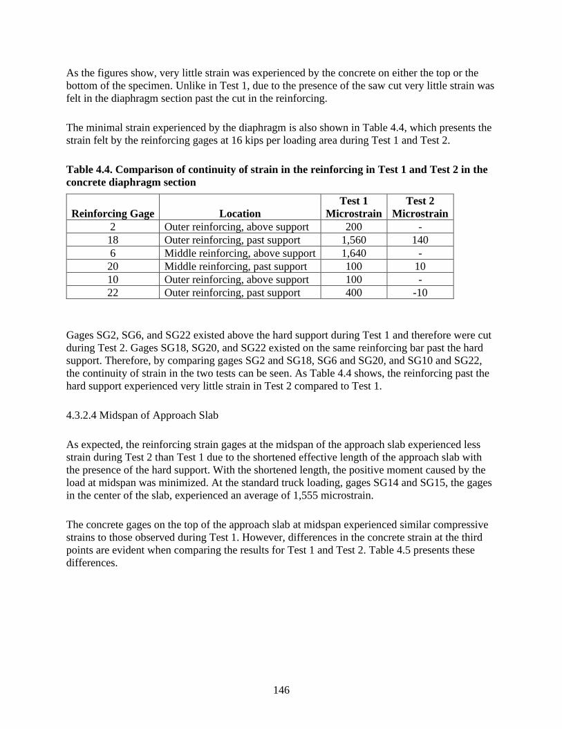
146
As the figures show, very little strain was experienced by the concrete on either the top or the
bottom of the specimen. Unlike in Test 1, due to the presence of the saw cut very little strain was
felt in the diaphragm section past the cut in the reinforcing.
The minimal strain experienced by the diaphragm is also shown in Table 4.4, which presents the
strain felt by the reinforcing gages at 16 kips per loading area during Test 1 and Test 2.
Table 4.4. Comparison of continuity of strain in the reinforcing in Test 1 and Test 2 in the
concrete diaphragm section
Reinforcing Gage Location
Test 1
Microstrain
Test 2
Microstrain
2 Outer reinforcing, above support 200 -
18 Outer reinforcing, past support 1,560 140
6 Middle reinforcing, above support 1,640 -
20 Middle reinforcing, past support 100 10
10 Outer reinforcing, above support 100 -
22 Outer reinforcing, past support 400 -10
Gages SG2, SG6, and SG22 existed above the hard support during Test 1 and therefore were cut
during Test 2. Gages SG18, SG20, and SG22 existed on the same reinforcing bar past the hard
support. Therefore, by comparing gages SG2 and SG18, SG6 and SG20, and SG10 and SG22,
the continuity of strain in the two tests can be seen. As Table 4.4 shows, the reinforcing past the
hard support experienced very little strain in Test 2 compared to Test 1.
4.3.2.4 Midspan of Approach Slab
As expected, the reinforcing strain gages at the midspan of the approach slab experienced less
strain during Test 2 than Test 1 due to the shortened effective length of the approach slab with
the presence of the hard support. With the shortened length, the positive moment caused by the
load at midspan was minimized. At the standard truck loading, gages SG14 and SG15, the gages
in the center of the slab, experienced an average of 1,555 microstrain.
The concrete gages on the top of the approach slab at midspan experienced similar compressive
strains to those observed during Test 1. However, differences in the concrete strain at the third
points are evident when comparing the results for Test 1 and Test 2. Table 4.5 presents these
differences.

147
Table 4.5. Concrete strain along approach slab at standard truck loading, Test 1 and Test 2
Concrete Gage Location Test 1 Microstrain Test 2 Microstrain
2/3 First third point 10 -150
4/5 Midspan -210 -260
6/7 Second third point 0 0
As the table shows, the first third point of the approach slab is in tension due to the negative
moment in Test 1. However, because of the presence of the hard support and the cut in the top
reinforcing, the entirety of the approach slab was in positive moment in Test 2, causing the first
third point to experience compression.
4.4 Finite Element Modeling
Two finite element models were developed for comparison with the laboratory results, each
model corresponding to either the Test 1 or Test 2 conditions. A brief overview pertaining to the
characteristics of the finite element models is provided next.
4.4.1 Finite Element Model Characteristics
4.4.1.1 Element Types
To model the geometry of the laboratory specimens, three-dimensional solid shapes were used
for the concrete slab and steel girders. The steel reinforcing was modeled using wire shapes, with
an associated cross-sectional area that matched that of the #5 or #6 reinforcing steel bars where
applicable. Hex elements were utilized for the three-dimensional shapes to ensure accurate
results and reduce computational time. A linear 3D truss element was utilized to model the wire
elements. A mesh size of 2 in. was utilized to model all parts.
4.4.1.2 Material Properties
4.4.1.2.1 Concrete
The elastic material properties for the concrete included the mass density, Poisson’s ratio, and
modulus of elasticity. The mass density was based on a typical density of 150 lb/ft3. The
modulus of elasticity was based on an average compressive strength of 5.2 ksi, obtained from
cylinder tests completed at the time of testing. The lower of the strengths from the bridge deck
and the approach slab was used. Hsu and Hsu (1994) stated that the ACI 318-14 building code
overestimates the modulus of elasticity with the typical equation 57,000√𝑓′𝑐. Therefore, an
adjusted modulus of elasticity was used.
𝐸0 = 1.2431 ∗ 102𝑓′𝑐
+ 3.28312 ∗ 103 (1)

148
Using this equation, the modulus of elasticity utilized in the model was 3,919.1 ksi. The
Poisson’s ratio was taken as 0.15.
Hsu and Hsu’s (1994) model was used to generate the nonlinear stress-strain behavior for the
concrete. Unlike other models developed, Hsu and Hsu’s (1994) model only relies on the
compressive strength of the concrete. As shown in Figure 4.39, concrete follows a linear stress-
strain relationship corresponding to its maximum compressive strength, 𝑓′𝑐.
Hsu and Hsu 1994
Figure 4.39. Compression stress-strain curve
Hsu and Hsu’s (1994) model begins at 0.5𝑓′𝑐 and ends when the stress descends to 0.3𝑓′𝑐.
Between these points, equation (6) describes the compressive stress values:
𝑓𝑐 = (𝛽(
𝜀𝑐𝜀𝑜
⁄ )
𝛽−1+(𝜀𝑐
𝜀𝑜⁄ )
)𝑓′𝑐 (6)
where
𝛽 =1
1−[𝑓′
𝑐𝜀𝑜𝐸𝑜
⁄ ] (7)
and
𝜀𝑜 = 8.9 ∗ 10−5𝑓′𝑐
+ 2.114 ∗ 10−3 (8)
The inelastic strain of the concrete, 𝜀𝑐𝑖𝑛, is equivalent to the total strain, 𝜀𝑐, minus the elastic
strain, calculated as follows:

149
𝜀𝑐𝑖𝑛 = 𝜀𝑐 −
𝑓′𝑐
𝐸𝑜 (9)
A damage factor was be used to represent the degradation of the elastic stiffness of the system
and is calculated using the following equation:
𝑑 = 1 −𝑓𝑐
𝑓′𝑐 (10)
The relationship between the elastic modulus and the compressive damage factor is as follows:
𝐸 = (1 − 𝑑)𝐸𝑜 (11)
To capture the tension stiffening in the concrete, the Nayal and Rasheed (2006) model, modified
by Wahalathantri et al. (2011), was used. Similar to the concrete compressive parameters, both
the nonlinear stress-strain behavior and the tensile damage were defined. Figure 4.40 shows the
tensile behavior of the concrete.
Wahalathantri et al. 2011
Figure 4.40. Tension stress-strain curve
The concrete behavior is linear until reaching the maximum tensile stress, 𝑓𝑡𝑜, corresponding to
the cracking strain, 𝜀𝑐𝑟 . Then, the stress decreases until 0.77𝑓𝑡𝑜, corresponding to 1.25𝜀𝑐𝑟. The
stress decreases additionally to 0.45𝑓𝑡𝑜, corresponding to 4𝜀𝑐𝑟, until reaching 0.1𝑓𝑡𝑜,
corresponding to 8.7𝜀𝑐𝑟. The maximum tensile stress was calculated using 7.5√𝑓′𝑐 and Hooke’s
Law. The tension damage parameters were calculated in a fashion similar to that for the
compression parameters.
Figure 4.41 describes the relationship between the compressive and tensile stress and the
compressive and tensile damage, respectively.

150
Dassault Systemes SIMULIA Abaqus 2013
Figure 4.41. Relationship between tension (a) and compression (b) stress-strain response
and damage
In addition to the stress-strain tension and compression models, the following properties were
utilized in the FE model:
• Dilation angle: 31°
• Eccentricity: 0.1
• Ratio of biaxial strength to uniaxial strength, 𝑓𝑏𝑜/𝑓𝑐𝑜: 1.16
• Ratio of the second stress invariant on tensile meridian, K: 0.667
• Viscosity parameter: 0.0005
4.4.1.2.2 Steel
Only elastic properties were defined for the reinforcing steel and the steel girders because both of
these components were expected to stay in their elastic range during testing. A modulus of
elasticity of 29,000 ksi and a Poisson’s ratio of 0.19 was utilized for both.

151
4.4.1.3 Boundary Conditions and Constraints
The boundary conditions were the same in both FE models. As shown in Figure 4.42, the
bottoms of the steel girders were fixed.
Figure 4.42. Boundary conditions in both the Test 1 and Test 2 FE models
Six inches in from the edge of the approach slab, a boundary condition restrained movement in
the y direction, simulating a roller support.
Constraints were added to both models by tying the top of the steel girder to the bottom of the
concrete resting against those girders. This is shown in Figure 4.43.
Figure 4.43. Constraints and the unbonded construction joint in the FE model
Additionally, the reinforcing was embedded into the concrete element.
For Test 2, a hard support was inserted under the approach slab, and the top concrete cover and
reinforcing steel was cut centered above the support. The edge of the hard support was
constrained to the bottom of the approach slab as shown in Figure 4.44.

152
Figure 4.44. Test 2 FE model with added elements
The bottom of the hard support was fixed, preventing it from moving translationally or
rotationally. Besides these changes for Test 2, all other constraints and boundary conditions were
kept the same as in Test 1.
4.4.2 FE Model versus Experimental Results
Figure 4.45 shows the deflection along the length of the span for the FE model compared to the
results for Test 1.
Figure 4.45. Comparison between the FE model and the experimental results for deflection
along the length of specimen, Test 1
As the figure shows, the results for Test 1 are fairly consistent with the FE model throughout.
With these consistent results, more accurate results can be confidently inferred by simulating
Test 2 with further FE analyses. Such FE simulations may produce more credible results in
comparison to the laboratory test using the cracked specimen.
Cracking patterns in the finite element model are shown through tensile damage parameters.
Cracking patterns for the FE models of the specimen are presented in Figure 4.46 through Figure
4.49.

153
Figure 4.46. Tensile damage on the top of the specimen, Test 1
Figure 4.47. Tensile damage on the bottom of the specimen, Test 1
Figure 4.48. Tensile damage on the top of the specimen, Test 2

154
Figure 4.49. Tensile damage on the bottom of the specimen, Test 2
The figures show that the cracking patterns in the FE models for Test 1 closely resemble those
experienced by the specimen during the laboratory experiment. Fortunately, through FE
modeling, the cracking that would occur during Test 2 can be more accurately predicted. As
shown, no cracking is experienced by the top of the specimen in the FE simulation for Test 2,
specifically in the existing bridge section, due to the release of stress at the saw cut. Overall, the
tensile damage is similar on the bottom of the specimen between the Test 1 and Test 2 FE
models. However, the cracks in the Test 1 model do extend slightly further along the length of
the specimen, and the cracks in the Test 2 model are spaced more closely together. Both of these
observations are due to the presence of the hard support representing the backwall for Test 2
only.
This same pattern can be seen in Figure 4.50, which presents the distribution of E11 strain along
the length of the specimen for the Test 1 and Test 2 FE models.

155
Figure 4.50. Strain (E11) in the concrete along the length of the specimen, Test 1 (top) and
Test 2 (bottom)
Similar to the results described above, the figure shows that the stress on the bottom of the slab is
more concentrated in Test 2 than in Test 1 Additionally, the stress concentration in the
diaphragm and bridge deck sections in Test 2 is in the saw cut area, whereas in Test 1 it is not.
Figure 4.51 shows the same strain in the reinforcing along the length of the specimen for Test 1
and Test 2 FE models.

156
Figure 4.51. Strain (E11) in the reinforcing along the length of the specimen, Test 1 (top)
and Test 2 (bottom)
The Test 1 model has a larger stress concentration at the midspan of the approach slab compared
to the Test 2 model. However, a new stress concentration formed above the hard support in Test
2 due to the high strain experienced by the bottom reinforcing. Moreover, the reinforcing is
carrying stress into the bridge deck in Test 1, whereas in Test 2 the stress is released before this
point.
Similar to the observations regarding the cracking experienced by the laboratory specimen
during testing, the FE model for Test 2 shows a very large stress concentration near the saw cut
and hard support. During laboratory testing, cracks propagated from the bottom of the saw cut to
the bottom of the approach slab. Figure 4.52(a) shows similar cracking occurring in the FE
model for Test 2. Figure 4.52(b) shows the stress occurring in this area.

157
Figure 4.52. Cracking (a) and stress concentration (b) at the saw cut and hard support,
Test 2
The figure shows that a large stress concentration occurred where the approach slab was resting
on the corner of the hard support. Because the slab had rotated, only a small part of the specimen
was resting on this corner, causing a large stress concentration. The weakness of the saw cut,
coupled with an increase in stress directly below, naturally caused cracking to occur at this
location.

158
CHAPTER 5. COST ANALYSIS
An estimate of the installation and repair or replacement costs over the service life of a bridge
was developed for various types of joints, including the deck over backwall concept. In addition,
the construction costs of the Iowa DOT’s design for the deck over backwall concept (shown in
Figure 1.3 through Figure 1.5) were estimated using the Iowa DOT’s Final Bridge Design
software. With the cost estimate over the service life of a bridge and the construction cost of the
concept, the implementation of the bridge over backwall concept was compared that of other
joint types.
5.1 Background
To develop the cost estimate, a service life and a cost associated with each type of joint was
needed. As part of a study for the Massachusetts DOT (MassDOT), Civjan and Quinn (2016)
researched the best practices for bridge expansion joints and headers in the northeastern states of
the US. The authors surveyed MassDOT and several neighboring DOTs on their use of
expansion joints and, more particularly for this research, the service life of each type of joint.
The nine states surveyed were Connecticut, Maine, Massachusetts, New Hampshire, New Jersey,
New York, Pennsylvania, Rhode Island, and Vermont. Table 5.1 shows the responses from the
nine states in terms of the service life for the various types of joints.
Table 5.1. Typical service life of joints
Civjan and Quinn 2016
SS:D = Saw and Seal Deck over Backwall; SS:O = Saw and Seal over EM-SEAL; APJ = Asphalt Plug Joint; CS =
Compression Seal; SS = Strip Seal; EM = EM- SEAL; PS = Pourable Seal; MJ = Modular Joint; SPJ = Sliding Plate
Joint; FJ = Finger Joint; OJ = Open Joint; LS = Link Slab
Civjan and Quinn (2016) compiled the service life of the various types of joints from the
responses of the nine states and categorized them in ranges from 0 to 4 years, 5 to 8 years, 9 to
12 years, 13 to 16 years, and over 16 years.
Civjan and Quinn (2016) also provided typical costs in cost per linear foot in US dollars ($) for
the installation of the various joint types. For the cost estimate developed in the following pages,
the installation cost for all joints was assumed to be the same as the repair or replacement cost
with the exception of Strip Seal, where the installation cost was taken as $300 to $800 per linear
foot while the repair or replacement cost was taken as $75 per linear foot. These costs are listed
alongside the different types of joints in Table 5.2.

159
Table 5.2. Typical cost of joints
Civjan and Quinn 2016
The cost for three types of joints was not provided: Sliding Plate Joints, Open Joints, and Link
Slabs. In the service life study and the cost estimate detailed in the following pages, these types
of joints were omitted because a direct comparison in terms of cost could not be established.
As the table shows, the cost of Saw and Seal Deck over Backwall is extremely low, $15 to $25
per linear foot, compared to the rest of the joint types. The saw and seal detailing can be seen in
the joint developed by the Iowa DOT described in Chapter 4, Figure 4.1. The highest costs listed
are for Finger Joints, with costs of $1,375 to $1,750 per linear foot, and Modular Joints, with
costs of $1,750 to $4,600 per linear foot.
To develop the cost estimate, three different cost points were determined for each joint: low,
average, and high. The lowest cost of each type of joint corresponds to the low cost point, the
average cost to the average cost point, and the highest cost to the high cost point. For example,
for the Asphalt Plug Joint, the low cost would be $20 per linear foot, the average cost would be
$160 per linear foot, and the high cost would be $200 per linear foot. Some of the joint types
have the same value for all three cost points, for example, Pourable Seal, Compression Seal,
Strip Seal replacement, Saw and Seal over EM-SEAL, and EM-SEAL.
5.2 Service Life of Joints
As seen in Table 5.1, each type of joint listed has various values for its service life. To develop
the cost estimate, the service life of each type of joint was studied in relation to the bridge
service life. The aim was to find the number of times the joint has to be repaired or replaced in
the service life of the bridge. A variable bridge service life of 25 years or 50 years was used.
Three different service life values were determined for each joint: early, average, and late. For
the early service life of each joint, the lowest value of the range in Table 5.1 was used to
determine the average service life. For example, in the 5 to 8 years range, 5 years of service life
was used for the early value. For the average service life of each joint, the average of the range
was used to determine the average service life. For the late service life of each joint, the highest
value of the range was used to determine the average service life. Some adjustments were made
in the process. For the over 16 years range, 16 years was used across all three stages. For

160
example, if the service life of particular joint was 20 years, the data for that joint would be
capped at 16 years. For the 0 to 4 years range, a minimum of 1 year was used for the early
service life since it is unrealistic for a joint to have a service life of 0 years.
Using the process detailed above, the number of repairs or replacements for each joint over a
bridge service life of 25 years or 50 years was determined. Every joint type starts with an
installation, and that was assumed to be equivalent to a repair or replacement in this study with
the exception of Strip Seal joints. Table 5.3 and Table 5.4 show the number of times each joint
has to be repaired or replaced for a bridge service life of 25 years and 50 years, respectively.
Table 5.3. Repairs or replacements over 25 years
Table 5.4. Repairs or replacements over 50 years
Each table has the three stages, early, average, and late, as described above for each joint type.
From the results presented in these tables, it can be recognized that the number of repairs or
replacements for Saw and Seal Deck over Backwall ranks among the lowest of the nine joint
types being studied. In contrast, the Pourable Seal joint has the highest number of repairs or
replacements. Generally, each type of joint can be ranked in terms of the number of repairs or
replacements as follows: Finger Joint and Modular Joint, Strip Seal and Saw and Seal Deck over
Early Average Late
2 2 2
14 8 5
3 3 3
3 3 2
3 3 2
6 4 4
6 5 4
2 2 2
4 3 3
Repair or ReplacementsJoint Type
Finger Joints
Asphalt Plug Joint
Pourable Seal
Compression Seal
Strip Seal
Modular Joint
EM-SEAL
Saw and Seal Deck over Backwall
Saw and Seal over EM-SEAL
Early Average Late
4 4 4
28 16 10
6 5 5
5 5 4
5 5 4
11 8 7
12 9 7
4 4 4
7 6 6
Repair or ReplacementsJoint Type
Finger Joints
Pourable Seal
Compression Seal
Strip Seal
Saw and Seal Deck over Backwall
Saw and Seal over EM-SEAL
Asphalt Plug Joint
Modular Joint
EM-SEAL

161
Backwall, Compression Seal, EM-SEAL, Saw and Seal over EM-SEAL, Asphalt Plug Joint, and
Pourable Seal. These numbers are used in the cost estimate described in the following sections.
5.3 Cost Estimate over Bridge Service Life
A cost estimate of the repair or replacement costs of various types of joints over a design service
life of a bridge of 25 years or 50 years was developed. Various factors were taken into account
for this analysis. The joint length would change with the bridge in question and therefore
influence the cost of each repair or replacement. The analysis was conducted for the two case
study bridges, the Story County bridge and the Marshall County bridge. The Story County bridge
has a roadway width of 30 ft and is a non-skewed bridge; therefore, the joint is taken as 30 ft. On
the other hand, the Marshall County bridge has a roadway width of 44 ft transversely, but the
joint is approximately 62 ft diagonally due to the skew of the bridge.
Another factor that was taken into account was the inflation rate. The inflation rate was assumed
as 2%, 3%, and 4% during the course of this analysis. Another factor that was considered was the
service life of each joint. As previously discussed, three different service life values were
determined for each joint: early, average, and late. The last factor that was taken into account
was the service life of the bridge itself; 25 years or 50 years was used for this variable.
Throughout the discussion, the indicators LE, LA, LL, AE, AA, AL, HE, HA, and HL are used.
The first letter refers to the repair or replacement cost used (low, average, or high) and the
second letter refers to the service life used (early, average, or late). For example, the designation
AE would mean an average cost with an early service life.
The future cost of repair or replacement of each joint at the end of its service life was determined
using equation (12).
𝐹𝑉 = 𝑃𝑉 × (1 + 𝑖)𝑁 (12)
where FV is the future value, PV is the present value, i is the inflation rate, and N is the number
of periods.
To develop the cost estimate, the FV of the repair or replacement of the various types of joints
was calculated using PV as the cost of each type of joint shown in Section 5.1, Table 5.2, and N
as the service life of each type of joint discussed in Section 5.2, Table 5.3 and Table 5.4.
The results for the Marshall County bridge with an inflation rate of 2% and a bridge service life
of 25 years are shown in Figure 5.1 for AE, Figure 5.2 for AA, and Figure 5.3 for AL.

162
Figure 5.1. Marshall County bridge - 25 year service life, average cost, early service life
Figure 5.2. Marshall County bridge - 25 year service life, average cost, average service life

163
Figure 5.3. Marshall County bridge - 25 year service life, average cost, late service life
The results for a bridge service life of 50 years are shown in Figure 5.4 for AE, Figure 5.5 for
AA, and Figure 5.6 for AL.
Figure 5.4. Marshall County bridge - 50 year service life, average cost, early service life

164
Figure 5.5. Marshall County bridge - 50 year service life, average cost, average service life
Figure 5.6. Marshall County bridge - 50 year service life, average cost, late service life
Figures are not shown for the rest of the cases (the Story County bridge, other cost and service
life combinations, and other inflation rates). Each step in the graph represents a repair or

165
replacement cost. Each joint type begins with an installation cost in the present, or year 0. This
installation cost is assumed to be the same as the repair or replacement cost for all types of joints
except Strip Seal.
The costs for the Story County bridge are shown in Table 5.5, Table 5.6, Table 5.7, Table 5.8,
Table 5.9, and Table 5.10.
Table 5.5. Story County bridge - 25 year service life, 2% inflation rate
Table 5.6. Story County bridge - 50 year service life, 2% inflation rate
Table 5.7. Story County bridge - 25 year service life, 3% inflation rate
LE LA LL AE AA AL HE HA HL
97115 97378 97642 102740 103003 103267 108365 108628 108892
298007 159914 89288 298007 159914 89288 298007 159914 89288
65797 67723 69820 65797 67723 69820 65797 67723 69820
26401 26898 11926 43197 43915 19426 59993 60931 26926
2292 2341 1037 2631 2683 1187 2969 3025 1337
23103 13130 13855 23103 13130 13855 23103 13130 13855
44871 36574 27201 52032 42321 31402 59193 48068 35602
120751 121773 122809 163501 164523 165559 206251 207273 208309
20531 12940 13295 20531 12940 13295 20531 12940 13295
US Dollar ($)Joint Type
Finger Joints
Pourable Seal
Compression Seal
Strip Seal
Saw and Seal Deck over Backwall
Saw and Seal over EM-SEAL
Asphalt Plug Joint
Modular Joint
EM-SEAL
LE LA LL AE AA AL HE HA HL
406765 410168 413608 430325 433861 437435 453885 457554 461262
819095 459409 267887 819095 459409 267887 819095 459409 267887
225164 171813 183172 225164 171813 183172 225164 171813 183172
66962 70207 47600 109563 114622 77535 152164 159038 107469
5913 6182 4159 6786 7085 4760 7660 7989 5362
60384 40408 36140 60384 40408 36140 60384 40408 36140
131027 94412 69492 151939 109247 80223 172851 124082 90955
505764 512921 520216 684821 692989 701303 863878 873058 882391
52826 43060 46279 52826 43060 46279 52826 43060 46279
US Dollar ($)Joint Type
Finger Joints
Pourable Seal
Compression Seal
Strip Seal
Saw and Seal Deck over Backwall
Saw and Seal over EM-SEAL
Asphalt Plug Joint
Modular Joint
EM-SEAL
LE LA LL AE AA AL HE HA HL
106119 106575 107033 111744 112200 112658 117369 117825 118283
337950 181040 99860 337950 181040 99860 337950 181040 99860
72998 76356 80091 72998 76356 80091 72998 76356 80091
28771 29633 12330 46605 47835 19830 64438 66036 27330
2607 2694 1120 2968 3062 1270 3329 3429 1420
26322 14532 15796 26322 14532 15796 26322 14532 15796
50311 41441 30695 58165 47759 35251 66020 54076 39807
130170 131911 133691 172920 174661 176441 215670 217411 219191
23250 14223 14834 23250 14223 14834 23250 14223 14834
Modular Joint
EM-SEAL
Saw and Seal Deck over Backwall
Saw and Seal over EM-SEAL
Asphalt Plug Joint
Pourable Seal
Compression Seal
Strip Seal
Joint TypeUS Dollar ($)
Finger Joints

166
Table 5.8. Story County bridge - 50 year service life, 3% inflation rate
Table 5.9. Story County bridge - 25 year service life, 4% inflation rate
Table 5.10. Story County bridge - 50 year service life, 4% inflation rate
These tables vary in terms of the bridge service life (25 or 50 years) and the inflation rate (2%,
3%, or 4%). The tables are color coded, with red cells representing the higher cost values and
green cells representing the lower cost values. Each table shows all of the different cost and
service life combinations (LE, LA, LL, etc.).
The costs for the Marshall County bridge are shown in Table 5.11, Table 5.12, Table 5.13, Table
5.14, Table 5.15, and Table 5.16, varying the same factors.
LE LA LL AE AA AL HE HA HL
535431 542624 549936 563813 571264 578838 592194 599904 607739
1089052 614352 352402 1089052 614352 352402 1089052 614352 352402
298084 221395 245181 298084 221395 245181 298084 221395 245181
83388 89965 57586 135074 145224 92614 186761 200483 127642
7765 8336 5267 8840 9472 5973 9916 10607 6678
80094 52224 47907 80094 52224 47907 80094 52224 47907
172379 123574 90007 199291 142413 103368 226204 161252 116729
656782 671624 686903 872481 889286 906551 1088180 1106947 1126200
68965 55519 62269 68965 55519 62269 68965 55519 62269
Modular Joint
EM-SEAL
Saw and Seal Deck over Backwall
Saw and Seal over EM-SEAL
Asphalt Plug Joint
Pourable Seal
Compression Seal
Strip Seal
Joint TypeUS Dollar ($)
Finger Joints
LE LA LL AE AA AL HE HA HL
116465 117167 117875 122090 122792 123500 127715 128417 129125
337950 181040 99860 337950 181040 99860 337950 181040 99860
72998 76356 80091 72998 76356 80091 72998 76356 80091
28771 29633 12330 46605 47835 19830 64438 66036 27330
2607 2694 1120 2968 3062 1270 3329 3429 1420
26322 14532 15796 26322 14532 15796 26322 14532 15796
50311 41441 30695 58165 47759 35251 66020 54076 39807
130170 131911 133691 172920 174661 176441 215670 217411 219191
23250 14223 14834 23250 14223 14834 23250 14223 14834
Joint TypeUS Dollar ($)
Finger Joints
Pourable Seal
Compression Seal
Strip Seal
Saw and Seal Deck over Backwall
Saw and Seal over EM-SEAL
Asphalt Plug Joint
Modular Joint
EM-SEAL
LE LA LL AE AA AL HE HA HL
716040 729655 743578 750624 764684 779062 785207 799714 814545
1468563 833705 469895 1468563 833705 469895 1468563 833705 469895
400492 288990 333581 400492 288990 333581 400492 288990 333581
105162 117084 70481 168552 186744 111826 231941 256403 153170
10346 11434 6753 11687 12882 7588 13027 14329 8423
107752 68327 64437 107752 68327 64437 107752 68327 64437
229846 163892 118058 264942 188122 134888 300038 212351 151718
865520 893103 921796 1128352 1159329 1191470 1391185 1425554 1461145
91238 72482 85153 91238 72482 85153 91238 72482 85153
Joint TypeUS Dollar ($)
Finger Joints
Pourable Seal
Compression Seal
Strip Seal
Saw and Seal Deck over Backwall
Saw and Seal over EM-SEAL
Asphalt Plug Joint
Modular Joint
EM-SEAL

167
Table 5.11. Marshall County bridge - 25 year service life, 2% inflation rate
Table 5.12. Marshall County bridge - 50 year service life, 2% inflation rate
Table 5.13. Marshall County bridge - 25 year service life, 3% inflation rate
Table 5.14. Marshall County bridge - 50 year service life, 3% inflation rate
LE LA LL AE AA AL HE HA HL
201435 201979 202527 213102 213647 214194 224769 225314 225861
618119 331691 185200 618119 331691 185200 618119 331691 185200
136476 140470 144819 136476 140470 144819 136476 140470 144819
54761 55791 24736 89599 91087 40293 124437 126383 55849
4754 4856 2152 5456 5565 2463 6159 6275 2774
47919 27233 28738 47919 27233 28738 47919 27233 28738
93070 75862 56420 107923 87782 65133 122777 99702 73846
250460 252578 254728 339131 341250 343399 427803 429921 432071
42585 26840 27575 42585 26840 27575 42585 26840 27575
Modular Joint
EM-SEAL
Saw and Seal Deck over Backwall
Saw and Seal over EM-SEAL
Asphalt Plug Joint
Pourable Seal
Compression Seal
Strip Seal
Joint TypeUS Dollar ($)
Finger Joints
LE LA LL AE AA AL HE HA HL
843703 850762 857896 892571 899906 907319 941439 949050 956741
1698951 952897 555646 1698951 952897 555646 1698951 952897 555646
467030 356372 379931 467030 356372 379931 467030 356372 379931
138891 145621 98730 227253 237747 160821 315615 329874 222911
12265 12822 8627 14076 14696 9874 15887 16570 11121
125248 83813 74962 125248 83813 74962 125248 83813 74962
271774 195827 144139 315149 226598 166398 358524 257368 188657
1049045 1063891 1079021 1420441 1437385 1454629 1791838 1810879 1830237
109571 89315 95990 109571 89315 95990 109571 89315 95990
Modular Joint
EM-SEAL
Saw and Seal Deck over Backwall
Saw and Seal over EM-SEAL
Asphalt Plug Joint
Pourable Seal
Compression Seal
Strip Seal
Joint TypeUS Dollar ($)
Finger Joints
LE LA LL AE AA AL HE HA HL
220110 221055 222007 231777 232722 233674 243444 244389 245341
700970 375510 207128 700970 375510 207128 700970 375510 207128
151411 158375 166124 151411 158375 166124 151411 158375 166124
59677 61465 25575 96667 99218 41131 133656 136971 56687
5406 5589 2323 6155 6350 2634 6904 7112 2945
54597 30143 32764 54597 30143 32764 54597 30143 32764
104353 85956 63666 120645 99060 73117 136938 112164 82567
269996 273607 277299 358667 362278 365971 447338 450949 454642
48224 29501 30768 48224 29501 30768 48224 29501 30768
Modular Joint
EM-SEAL
Saw and Seal Deck over Backwall
Saw and Seal over EM-SEAL
Asphalt Plug Joint
Pourable Seal
Compression Seal
Strip Seal
Joint TypeUS Dollar ($)
Finger Joints
LE LA LL AE AA AL HE HA HL
1110581 1125500 1140667 1169449 1184904 1200613 1228317 1244308 1260559
2258889 1274277 730946 2258889 1274277 730946 2258889 1274277 730946
618280 459212 508550 618280 459212 508550 618280 459212 508550
172961 186604 119444 280169 301221 192098 387376 415839 264753
16105 17291 10925 18336 19646 12388 20567 22001 13852
166129 108321 99368 166129 108321 99368 166129 108321 99368
357544 256315 186691 413366 295390 214404 469187 334466 242117
1362285 1393070 1424760 1809683 1844539 1880351 2257080 2296008 2335942
143047 115156 129157 143047 115156 129157 143047 115156 129157
Modular Joint
EM-SEAL
Saw and Seal Deck over Backwall
Saw and Seal over EM-SEAL
Asphalt Plug Joint
Pourable Seal
Compression Seal
Strip Seal
Joint TypeUS Dollar ($)
Finger Joints

168
Table 5.15. Marshall County bridge - 25 year service life, 4% inflation rate
Table 5.16. Marshall County bridge - 50 year service life, 4% inflation rate
The results of the cost analysis clearly show that Saw and Seal Deck over Backwall has the
lowest cost compared to all other types of joints and across all combinations of cost and service
life (LE, LA, LL, etc.). It also has the lowest cost whether the bridge service life is 25 years or 50
years. This can easily be recognized in the color-coded tables; the greenest cells in each table
correspond to Saw and Seal Deck over Backwall. From the other types of joints, Modular Joint,
Finger Joint, and Pourable Seal were identified as having the highest costs by a wide margin for
all of the cases shown. Saw and seal over EM-SEAL, Asphalt Plug Joint, Strip Seal, and EM-
SEAL ranked the lowest in terms of costs among the remaining types of joints.
5.4 Construction Cost of Deck over Backwall Concept
Various items were taken into consideration to develop an estimate of the construction cost of
the deck over backwall concept. The Iowa DOT’s Final Bridge Design software (Iowa DOT
Office of Bridges and Structures 2018b) was used to identify items that would pertain to the
construction cost of the Iowa DOT’s design for the deck over backwall concept. Specifically, a
spreadsheet titled Prepare Cost Estimate, last updated on April 25, 2017 (Iowa DOT Office of
Bridges and Structures 2018b), was used. This spreadsheet stores historical cost data for bid
items in state job estimates. Most items have cost data from May 2016 through April 2017, while
some items have cost data within the past 10 years
Figure 5.17 shows the items that were chosen in the software with the long bid and short bid
descriptions, measuring unit, unit price for each item, and date of the cost data.
LE LA LL AE AA AL HE HA HL
241569 243025 244494 253236 254692 256162 264903 266359 267829
797353 426423 232280 797353 426423 232280 797353 426423 232280
168514 179319 191608 168514 179319 191608 168514 179319 191608
65292 68053 26519 104649 108541 42075 144006 149030 57632
6178 6470 2515 6979 7289 2827 7779 8108 3138
62427 33444 37508 62427 33444 37508 62427 33444 37508
117321 97725 72093 135235 112172 82371 153149 126620 92648
291998 297464 303094 380669 386136 391765 469341 474807 480436
54811 32511 34451 54811 32511 34451 54811 32511 34451
Joint TypeUS Dollar ($)
Finger Joints
Pourable Seal
Compression Seal
Strip Seal
Saw and Seal Deck over Backwall
Saw and Seal over EM-SEAL
Asphalt Plug Joint
Modular Joint
EM-SEAL
LE LA LL AE AA AL HE HA HL
1485197 1513435 1542315 1556929 1586093 1615914 1628660 1658751 1689513
3046065 1729253 974646 3046065 1729253 974646 3046065 1729253 974646
830692 599418 691908 830692 599418 691908 830692 599418 691908
218125 242854 146190 349606 387340 231946 481087 531827 317703
21460 23716 14007 24240 26719 15739 27020 29722 17471
223496 141722 133654 223496 141722 133654 223496 141722 133654
476742 339942 244874 549537 390198 279783 622332 440454 314691
1795244 1852457 1911970 2340406 2404656 2471324 2885568 2956856 3030678
189245 150341 176623 189245 150341 176623 189245 150341 176623
Joint TypeUS Dollar ($)
Finger Joints
Pourable Seal
Compression Seal
Strip Seal
Saw and Seal Deck over Backwall
Saw and Seal over EM-SEAL
Asphalt Plug Joint
Modular Joint
EM-SEAL

169
Table 5.17. Deck over backwall concept construction items
Iowa DOT Office of Bridges and Structures 2018
The first item shown in the table is the excavation of Class 10 soil. According to the Iowa DOT
(2018), Class 10 soils include normal earth materials such as loam, silt, gumbo, peat, clay, soft
shale, sand, and gravel. It was determined that this class applies for most cases; therefore, it was
used in the estimate. The excavation extends 24 in. below the approach slab according to the
Iowa DOT Office of Design (2016). Placement of a new modified subbase was also considered
in the cost estimate. The design for the deck over backwall concept calls for the modified
subbase to be placed in the same volume that was excavated to support the new approach slab.
Using the bridge design standards from the Iowa DOT Office of Design (2016), the bridge
approach for the deck over backwall concept was estimated as having a cost similar to that of the
BR-205 approach slab, as shown in Table 5.17. Finally, concrete removal for the current
approach slab and the abutment interface was assumed for the length of the deck over backwall
concept and a 12 in. thickness.
Even though the Marshall County bridge was chosen as the test bridge where the deck over
backwall concept would be implemented, calculations were performed for both the Story County
bridge and the Marshall County bridge. A substantial difference in the estimate can be seen by
comparing a non-skewed bridge to a skewed bridge because different units of area and volume
lead to different cost estimates. The skew of the Marshall County bridge results in one end of the
approach slab being a 20 ft section and the other being a 64 ft section. This increases the cost
compared to non-skewed counterparts like the Story County bridge. A summary of the costs
associated with the deck over backwall concept is presented in Table 5.18 and Table 5.19 for the
Story County bridge and the Marshall County bridge, respectively.
Table 5.18. Story County bridge - construction cost of deck over backwall concept
Low High Average
2102-2710070 EXCAVATION, CLASS 10, ROADWAY AND BORROW CY 2 89.5 3.07 5-2016 thru 4-2017 EXCAVATION, CL 10, RDWY+BORROW
2115-0100000 MODIFIED SUBBASE CY 17 135 40.36 5-2016 thru 4-2017 MODIFIED SUBBASE
2301-0690205 BRIDGE APPROACH, BR-205 SY 150 190 174.06 5-2016 thru 4-2017 BRIDGE APPROACH, BR-205
2401-7207020 REMOVAL OF CONCRETE CY 267 267 267 12-2014 thru 10-2015 RMVL OF CONC
Date of Cost Data Short Bid Item Description
Unit Price ($)
UnitLong Bid Item DescriptionItem Code
Low High Average
EXCAVATION, CL 10, RDWY+BORROW 44.44 CY 136.44 2 89.5 3.07
MODIFIED SUBBASE 44.44 CY 1,793.78 17 135 40.36
BRIDGE APPROACH, BR-205 66.67 SY 11,603.88 150 190 174.06
RMVL OF CONC 22.22 CY 5,933.33 267 267 267
Total Cost ($) 19,467.44
Short Bid Item DescriptionTotal
QuantityUnit Total Cost ($)
Unit Price ($)

170
Table 5.19. Marshall County bridge - construction cost of deck over backwall concept
The average unit price from the Iowa DOT’s Final Bridge Design software was used for both
estimates.
The total construction cost of the deck over backwall concept was found to be approximately
$20,000 for the Story County bridge and $60,000 for the Marshall County bridge. The approach
slab itself, the cost of which was assumed to be equivalent to that of the BR-205 approach slab
from the Iowa DOT bridge design standards, accounts for more than half of the total construction
cost of the deck over backwall concept. Meanwhile, the concrete removal accounts for almost a
third of the cost, and the excavation and the modified subbase account for the other portions of
the construction cost.
From these total cost numbers, the impact of the skew on the approach slab costs can be
recognized. An almost 50% increase in roadway length, 44 ft for the Marshall County bridge
compared to 30 ft for the Story County bridge, with a 45° skew triples the construction cost of
the approach slab. This major difference is due to the larger area and volume requirements of an
approach slab with a skewed end in comparison to one with a non-skewed end. In comparison,
for other types of joints, the differences in the skew and the roadway length would more than
double the construction costs due to the relatively high cost of the expansion joint hardware and
materials, which are calculated per foot (62 ft for Marshall County and 30 ft for Story County).
Combining the repair or replacement costs of Saw and Seal Deck over Backwall and the
construction cost of the deck over backwall concept allows for a better comparison to be made to
other types of joints. The results for the Marshall County bridge are shown in Table 5.20 and
Table 5.21 for an inflation rate of 2% and in Table 5.22 and Table 5.23 for an inflation rate of
3%.
Table 5.20. Deck over backwall comparison, 25 year service life, 2% inflation rate
Low High Average
EXCAVATION, CL 10, RDWY+BORROW 136.89 CY 420.25 2 89.5 3.07
MODIFIED SUBBASE 136.89 CY 5,524.84 17 135 40.36
BRIDGE APPROACH, BR-205 205.33 SY 35,739.96 150 190 174.06
RMVL OF CONC 68.44 CY 18,274.67 267 267 267
Short Bid Item DescriptionTotal
QuantityUnit Total Cost ($)
Unit Price ($)
Total Cost ($) 59,959.71
LE LA LL AE AA AL HE HA HL
54761 55791 24736 89599 91087 40293 124437 126383 55849
64714 64815 62111 65416 65525 62423 66118 66235 62734
47919 27233 28738 47919 27233 28738 47919 27233 28738
93070 75862 56420 107923 87782 65133 122777 99702 73846
42585 26840 27575 42585 26840 27575 42585 26840 27575
Strip Seal
Joint TypeUS Dollar ($)
EM-SEAL
Saw and Seal Deck over Backwall
Saw and Seal over EM-SEAL
Asphalt Plug Joint

171
Table 5.21. Deck over backwall comparison, 50 year service life, 2% inflation rate
Table 5.22. Deck over backwall comparison, 25 year service life, 3% inflation rate
Table 5.23. Deck over backwall comparison, 50 year service life, 3% inflation rate
For each inflation rate, tables are presented for a bridge service life of 25 years and 50 years,
respectively. Only the comparable types of joints in terms of costs are shown. Four types of
joints (Finger Joint, Pourable Seal, Compression Seal, and Modular Joint) were omitted because
their costs were extremely high compared to the ones shown in the tables. The tables are color
coded in the same manner as those shown above.
The tables show that for a bridge service life of 25 years, the deck over backwall concept has a
higher cost than other comparable types of joints. The high initial cost accounts for most of the
costs, since the repair or replacement cost of Saw and Seal Deck over Backwall was found to be
the lowest among all types of joints by a wide margin. While the deck over backwall concept
might not be the best option in terms of cost for a bridge service life of 25 years, for a bridge
service life of 50 years, the deck over backwall concept has the lowest costs when compared to
all other types of joints across all combinations of cost point and service life (LE, LA, LL, etc.).
It should be noted that much of the cost of the saw and seal over backwall alternative is
associated with the removal and construction of the bridge approach. If the bridge approach
requires replacement in any case, an analysis would be much more likely to favor the saw and
seal over backwall alternative.
LE LA LL AE AA AL HE HA HL
138891 145621 98730 227253 237747 160821 315615 329874 222911
72224 72782 68586 74036 74656 69834 75847 76530 71081
125248 83813 74962 125248 83813 74962 125248 83813 74962
271774 195827 144139 315149 226598 166398 358524 257368 188657
109571 89315 95990 109571 89315 95990 109571 89315 95990
US Dollar ($)
Strip Seal
Joint Type
EM-SEAL
Saw and Seal Deck over Backwall
Saw and Seal over EM-SEAL
Asphalt Plug Joint
LE LA LL AE AA AL HE HA HL
59677 61465 25575 96667 99218 41131 133656 136971 56687
65366 65549 62282 66115 66310 62593 66864 67071 62905
54597 30143 32764 54597 30143 32764 54597 30143 32764
104353 85956 63666 120645 99060 73117 136938 112164 82567
48224 29501 30768 48224 29501 30768 48224 29501 30768EM-SEAL
Saw and Seal Deck over Backwall
Saw and Seal over EM-SEAL
Asphalt Plug Joint
Strip Seal
Joint TypeUS Dollar ($)
LE LA LL AE AA AL HE HA HL
172961 186604 119444 280169 301221 192098 387376 415839 264753
76065 77250 70885 78296 79606 72348 80526 81961 73812
166129 108321 99368 166129 108321 99368 166129 108321 99368
357544 256315 186691 413366 295390 214404 469187 334466 242117
143047 115156 129157 143047 115156 129157 143047 115156 129157EM-SEAL
Saw and Seal Deck over Backwall
Saw and Seal over EM-SEAL
Asphalt Plug Joint
Strip Seal
Joint TypeUS Dollar ($)

172
5.5 Break-Even Point Analysis
As demonstrated above for the Marshall County bridge, the deck over backwall concept
produced the lowest costs for a bridge service life of 50 years. In contrast, it did not rank as the
best alternative for a bridge service life of 25 years. Because of this, a break-even point (BEP)
between a bridge service life of 25 years and 50 years was identified. Beyond that point, the deck
over backwall concept would produce the lowest costs among all other types of joints across all
combinations of cost point and service life. Figure 5.7, Figure 5.8, and Figure 5.9 show the cost
estimate graphs presented above for the Marshall County bridge with an interest rate of 2% but
with the vertical axis limited to $100,000 so that the BEP can more easily be identified.
Figure 5.7. Break-even point - average cost, early service life

173
Figure 5.8. Break-even point - average cost, average service life
Figure 5.9. Break-even point - average cost, late service life
Table 5.24 presents the BEP for the Marshall County bridge across all different combinations of
cost point and service life for interest rates of 2%, 3%, and 4%. The average BEP for each
interest rate is also shown.

174
Table 5.24. Break-even point of deck over backwall concept
As the table shows, the BEP for the deck over backwall concept ranges from 31 years to 50
years. Some BEPs are calculated at exactly 50 years because the particular type of joint that
would be comparable to the deck over backwall concept would need a repair or replacement in
that same year. The lowest BEP that was obtained in the study was 31 years for 4 of the 27
different cases considered. The average BEP is shown for all three interest rates used in the
analysis. The average BEPs were 44 years, 38 years, and 36 years for interest rates of 2%, 3%,
and 4%, respectively. From these results, it can be concluded that as the interest rate increases,
the BEP decreases. In this analysis, the interest rate does not affect the initial construction cost of
the deck over backwall concept. Since the repair or replacement costs of Saw and Seal Deck over
Backwall were the lowest among the various types of joints, as the interest rate increases, all
repair or replacement costs for the other types of joints would increase more than the costs of
Saw and Seal Deck over Backwall.
5.6 Summary and Discussion
To develop a cost analysis comparing the deck over backwall concept and various types of joints,
pertinent information was used from Civjan and Quinn (2016) regarding the service life and
installation costs of several types of joints. Both variables, service life and installation costs,
were varied throughout the development of the cost estimates. Using the information from
Civjan and Quinn (2016), three service life values were determined for each type of joint: early,
average, and late. The installation and repair or replacement costs of each joint were also varied
throughout the study, with three different cost points determined for each type of joint: low,
average, and high. Other factors were also varied during the cost analysis. The interest rates used
were 2%, 3%, and 4%, though results are only presented for 2% and 3%. In addition, cost
analyses were conducted for both the Story County bridge and the Marshall County bridge, even
though the majority of the results presented correspond to the Marshall County bridge.
Cost estimates for nine different types of joints were developed based on the number of times
each type of joint must be repaired or replaced during the service life of the bridge. The
installation costs were assumed to be the same as the repair or replacement costs for each type of
joint except Strip Seals. Two different service lives, 25 years and 50 years, were used throughout
the study. The results from this estimate show that Saw and Seal Deck over Backwall produced
the lowest repair or replacement costs among all nine joints for all different interest rates (2%,
3%, and 4%), for both bridges under investigation (Story County bridge and Marshall County
bridge), and for all combinations of cost point and service life (LE, LA, LL, etc.).
The initial construction cost of the Iowa DOT’s design for the deck over backwall concept was
estimated. The Iowa DOT’s Final Bridge Design software was used to estimate the construction
Interest Rate LE LA LL AE AA AL HE HA HL Average
2% 38 44 50 38 44 50 38 44 50 44
3% 33 38 40 31 38 48 31 38 48 38
4% 33 35 40 31 38 40 31 38 40 36
Break-Even Point (Years)

175
cost using comparable bid items. The total construction cost of the deck over backwall concept
was found to be approximately $20,000 for the Story County bridge and $60,000 for the
Marshall County bridge. Skew was found to have a significant impact on cost, in that an
approach slab with a skewed end has a much greater length and area than an approach slab with a
non-skewed end.
The construction cost was incorporated into the repair or replacement cost estimates previously
discussed. The results show that for a bridge service life of 25 years, the deck over backwall
concept has a higher cost than other comparable types of joints. The high initial cost accounts for
most of the cost, since the repair or replacement cost of Saw and Seal Deck over Backwall was
found to be the lowest among all types of joints. For a bridge service life of 50 years, the Saw
and Seal Deck over Backwall concept has the lowest costs when compared to all other types of
joints across all combinations of cost point and service life. Because of this, a BEP between a
bridge service life of 25 years and 50 years was identified. Beyond that point, the deck over
backwall concept would produce the lowest costs among all other types of joints across all
combinations of cost point and service life. The results show that as the interest rate increases,
the BEP decreases. The average BEPs were 44 years, 38 years, and 36 years for interest rates of
2%, 3%, and 4%, respectively. The BEP for the deck over backwall concept ranges from 31
years to 50 years.
Many assumptions and simplifications were made to estimate the costs of the various types of
joints. Numerous factors could have been incorporated to improve the accuracy of this analysis.
The costs of maintenance for the interaction between the abutment/bridge deck and the approach
slab were not taken into account, nor was the costs of maintenance for the steel girders, bearings,
reinforcement, etc. These factors, among many others, could affect the cost of the various types
of joints compared in this study. Ideally, all of these factors would increase the costs of all types
of joints uniformly. However, since the deck over backwall concept would not be composed of
an expansion joint in the abutment interface, some of the costs associated with these factors
could be greatly reduced, and, quite possibly, eliminated in their entirety.
In conclusion, if these factors are all taken into account, the type of joint whose costs would
increase the least would likely be Saw and Seal Deck over Backwall, which would further
increase the cost difference between this joint and the joint with the next lowest cost for any
particular combination of cost point and service life (LE, LA, LL, etc.). Moreover, most of the
cost of the Saw and Seal Deck over Backwall concept is associated with the removal and
replacement of the bridge approach panel. If this approach panel would need to be replaced in
any case, the analysis would be much more favorable for the Saw and Seal Deck over Backwall
concept.
While this cost analysis covered the critical elements of the construction process, many other
components could be factored into the analysis. Some of these components could be formwork
costs, labor costs, work zone costs, lane closure costs, mobilization costs, etc. These can all be
added to the construction costs of the deck over backwall concept. At the same time, these
components and many others could also be added to the installation and repair or replacement
costs of all types of joints investigated.

176
CHAPTER 6. CONSTRUCTION OBSERVATION AND POST-CONSTRUCTION
TESTING PLAN
In this chapter, a construction observation and post-construction testing plan was developed for
the deck over backwall joint developed by the Iowa DOT. An instrumentation plan was
developed with various types of sensors and equipment. A post-construction plan with various
truck loading cases was developed as well. The correlations between the results from future field
testing based on this plan and the predictions of the FE models described in Chapter 3 will serve
to calibrate and improve the accuracy of the FE models. The test results will also provide vital
information on the behavior of expansion joints and allow for their efficient design.
6.1 Joint Detailing
The joint developed by the Iowa DOT, detailed in Chapter 1 was designated as the deck over
backwall concept and was selected by Iowa DOT staff members for implementation in a future
Iowa DOT construction season. This joint design was used for the development of the
instrumentation and post-construction testing plans discussed in this chapter.
6.2 Instrumentation
The instrumentation plan developed for the deck over backwall concept consists of various types
of sensors and equipment. The instrumentation includes strain gages with temperature sensors,
monitoring plates for surveying data, surveying equipment, and gapmeters. Each sensor and
piece of equipment serves a purpose in obtaining real-world data to correlate with the FE results
discussed in Chapter 3.
Thiagarajan et al. (2013) detailed the Missouri DOT’s (MoDOT) experience with the field
performance of various types of bridge approach slab designs. Monitoring plates were
incorporated into MoDOT’s approach slabs to provide a smooth and flat surface to collect
accurate readings. The deflections of the approach slab can be monitored over time using
surveying equipment over these monitoring plates. The equipment is shown in Figure 6.1.

177
Thiagarajan et al. 2013
Figure 6.1. Surveying prism (left), total station (right)
Detailed information on how to embed the monitoring plates is provided in Figure 6.2.
Thiagarajan et al. 2013
Figure 6.2. Monitoring plate details
In discussions between the research team for the present project and the Iowa DOT, the option of
using vertical reinforcement bars embedded into the concrete was brought up as an alternative to
using monitoring plates. The main advantage in using monitoring plates is that the plates would
not be chipped away by snowplow strikes or traffic loads. However, the rebar option could be
implemented as well because surveying data can be collected at the same points. It is
recommended that monitoring plates or vertical rebars be placed at nine points of interest on an
approach slab, as shown in Figure 6.3.

178
Figure 6.3. Monitoring plate distribution
It is also recommended that gapmeters be incorporated between the girders and the abutment
stud wall. These sensors would monitor the displacement of the girders at a certain height in the
longitudinal direction. With these data, the rotation of the girders can also be monitored.
A total of 13 strain gage locations are recommended. Nine of these strain gage locations are
recommended across the abutment interface, four at the midspan of the transverse spans and five
across each girder support. Four additional strain gage locations are recommended at the
midspan of the approach slab. This arrangement can be viewed in more detail on the
instrumentation plan shown in Figure 6.4.

179
SG: strain gage (13 locations); MP: monitoring plate (8 locations); GM: gapmeter (5 girders)
Figure 6.4. Instrumentation plan
Both top and bottom reinforcement bars can be fitted with strain gages. Multiple strain gages
should be used at each location because of the possibility that a certain number of strain gages
may malfunction due to improper installation or construction damage. The strain gages can be
used to monitor stress levels at the desired locations of the joint and approach slab over time.
6.3 Truck Loading Cases
Various truck loading allocations were considered for the post-construction testing of the deck
over backwall concept. For the purposes of this research and for continuity’s sake, HS20-44
truck loading conditions are recommended for this plan. These truck loads are shown in Chapter
3, Figure 3.56, Figure 3.57, Figure 3.58, and Figure 3.59, for the FE model of the Marshall
County bridge with the approach slab. During the discussion that follows, the middle and rear
axles of the trucks are used for allocation purposes. Therefore, even if a different truck with
different dimensions and tire spacing is used in the real-world simulations, these same axles can
be used for the truck allocations.
The various recommended truck cases can be seen in Figure 6.5, Figure 6.6, Figure 6.7, and
Figure 6.8 as Case 1, Case 2, Case 3, and Case 4, respectively.

180
Figure 6.5. Truck loading Case 1
Figure 6.6. Truck loading Case 2

181
Figure 6.7. Truck loading Case 3
Figure 6.8. Truck loading Case 4
Case 1 would have a larger maximum effect on the abutment and bearings of a non-skewed
bridge in comparison to a skewed bridge. That is because both wheels of the rear axle are closer
to the abutment on a non-skewed bridge in comparison to a skewed bridge when the load is
placed near the middle of the approach slab. For this case, the rear axle of the truck would be
located at the midspan of the 20 ft edge of the new approach slab. Case 2 corresponds to two
trucks back to back at the midspan of the 64 ft edge of the approach panel. This would maximize

182
deflection values and stress levels in the approach slab. Case 3 corresponds to two trucks side by
side with the rear axles close to the abutment interface. This would maximize the live load
abutment reactions while causing deflection at the abutment interface. Case 4 corresponds to two
trucks side by side at the midspan of the 64 ft edge and at the center of the approach slab. This
would provide high midspan deflection values and stress levels while adding to the live load
abutment reactions of both the exterior and interior supports, thereby adding live loads to the
bearing loads.

183
CHAPTER 7. CONCLUSIONS AND FUTURE WORK
The objectives of the research set out in Chapter 1 were accomplished. Conclusions were drawn
from each chapter, and possible avenues of future work were recommended. These conclusions
and recommendations are discussed in detail in this chapter.
7.1 Joint Detailing
Further development of the deck over backwall concept was accomplished in Chapter 3. The
research team proposed various options, with many alternatives considered by the research team
and the Iowa DOT. The Iowa DOT developed a joint taking into account the options presented
by the research team and various other factors.
While the Iowa DOT might move forward with the joint it developed, further detailing should be
developed regarding the deck over backwall concept. Various options remain for several of the
joints in the Iowa DOT joint and bridge approach panel detailing, such as selecting exactly where
a joint or saw cut might be placed in relation to the abutment backwall and the possibility of
moving the joint 15 ft from the abutment backwall. Possible options to include with this concept
are sleeper slabs, subdrains, EF joints, CF joints, CD joints, or any combination of these.
Consideration could also be given to whether to replace the fill under the approaches and correct
possible underdrain deficiencies.
Prior to selecting the aforementioned details, it would be desirable to contact the Michigan
Department of Transportation and New York State Department of Transportation to ascertain
whether further information is available regarding the performance of their deck over backwall
concept approach panels and how such information might improve Iowa DOT designs.
7.2 Finite Element Modeling and Analysis
Full-scale FE models of two different bridges, one non-skewed bridge in Story County and one
skewed bridge in Marshall County, were developed and detailed in Chapter 3. These models
were analyzed with various loading conditions from dead loads, temperature loading, and live
loads corresponding to various truck loading cases. Both models were validated using the
original drawing plans. The same process of modeling was used for both models in terms of
material properties, boundary conditions, constraints, loading conditions, and other factors.
The impact of the deck over backwall concept was studied with the Marshall County bridge
model, which showed an increase in bearing loads due to the additional dead load of the
approach slab and in live loads with the truck loading conditions. Relevant deflection values and
stress levels at various points of interest across the abutment interface and the midspan of the
approach slab were also determined. These FE results provide the Iowa DOT with a case study
example that will aid in the further development of the deck over backwall concept and possibly
a detailed design for a test installation.

184
A parametric study of various bridge skew angles (no skew, 30°, 45°, and 60°) was also
conducted with the Marshall County bridge. The results for models without soil support show
that generally the increase in the bridge skew angle leads to increased loads at the points of
interest under this study: the dead load abutment reactions and temperature deformation of the
bridges with and without the approach slab, the live load abutment reactions, and the deflection
values and stress levels at the abutment interface and in the midspan of the approach slab. The
results for models with soil support show more variance and do not follow a general trend due to
several factors. With these models, future correlations between the models and possible future
laboratory and field measurements can be accomplished.
While these models served the purpose of this research to study and develop the deck over
backwall concept, further analysis might also be desirable. Incorporating the steel bar
reinforcement and studying its behavior at the abutment interface and at the midspan of the
approach slab could be beneficial and provide more information for future designs of the deck
over backwall concept. In addition, a plastic analysis could also be performed under certain truck
loading conditions. The FE models were verified with loading conditions used at the time of the
original bridge design. While those loads are not entirely different from the loads used at the
time of writing, the FE models can be calibrated with current design loads. Further calibration of
the FE models would also be possible with the post-construction field testing. It should be noted
that further FE modeling would be desirable before selecting the concrete thickness and the
reinforcing configuration in the end diaphragm area and the longitudinal reinforcing for the
approach panels. Clarification of the exact removal limits for the abutment backwall location
would also be desirable; members of this project’s technical advisory committee noted that such
areas are often heavily deteriorated and require replacement under any circumstance.
Given the high loads that are predicted when the abutment is skewed but the sleeper slab that
supports the approach panel is not skewed, it would be desirable to consider designing the
sleeper slab so that it is parallel with the abutment. In doing so, the length that the approach
panel would have to bridge would be limited to 20 ft.
7.3 Experimental Investigation
An experimental laboratory investigation was completed, as discussed in Chapter 4. It was
discovered that cutting the top longitudinal reinforcing minimizes the stress that the bridge deck
experiences from the negative moment caused by loading. If not cut, cracks will form on the
surface of the bridge deck, possibly leading to harmful chemicals penetrating the interior of the
slab.
If the decision is made to cut the top longitudinal reinforcing, special care must be taken with the
filler material in the saw cut. The material should be able to withstand considerable stretching
and deformation. Additionally, the material should serve as a protective layer against the
cracking that could occur underneath the saw cut due to the increased stresses that form there.
Due to cracking and deformation, this saw cut could create a bump on the driving surface.
Cracking could be mitigated underneath the saw cut by moving the cut to the edge of the

185
backwall. When the saw cut is in the middle of the backwall, the rotation of the approach slab
causes stress to traverse from the contact point to the bottom of the saw cut, creating cracking.
The far end of the approach slab, independent of whether the top longitudinal reinforcing is cut,
will experience upward rotation. When designing the connection between the roadway and
approach slab, the engineer should take this rotation into account. The presence of a backwall
increases the moment capacity of the approach slab section due to a decrease in the effective
length. This, in turn, reduces the stresses in the midspan of the slab. If soil support is effective
underneath the approach slab, the stresses will be reduced, depending on the soil support
properties.
Additional testing can be performed for the deck over backwall concept. Various truck loading
cases can be tested for the approach slab. Variations in soil support could be incorporated into
the field testing plan for the approach slab. Soil compaction could be controlled to simulate the
three compositions (loose, moderately stiff, and stiff) considered in the FE model.
7.4 Cost Analysis
A comparison between the various types of joints and the deck over backwall concept in terms of
cost was performed and is documented in Chapter 5. When combining the repair or replacement
costs and the construction cost of the deck over backwall concept, the concept is the best
alternative among nine types of joints considered for a bridge service life of 50 years. For a
bridge service life of 25 years, the deck over backwall concept has a higher cost than other
comparable types of joints. For most cost point and service life scenarios considered, the concept
generally ranked between the third and fourth lowest cost out of the nine types of joints. The
high initial cost accounts for most of the concept’s life cycle costs, since the repair or
replacement costs were found to be the lowest among all types of joints by a considerable
margin. A BEP between 25 years and 50 years was identified to determine the point at which the
deck over backwall concept would produce the lowest costs among all other types of joints
across all combinations of cost point and service life. The results show that the BEP is 44 years
for a 2% interest rate and lowers as the interest rate increases.
Many assumptions and simplifications were made as part of the cost comparison. Numerous
factors could have been incorporated into the cost of installation, repair, replacement, and
construction of not only the deck over back wall concept but also the other types of joints
considered. A more in-depth cost analysis could be performed by taking into account additional
factors, such as the maintenance costs of the abutment interface, approach slab, steel girders,
bearings, and the steel reinforcement bars in the bridge deck and the abutment and the costs of
formwork, labor, work zones, lane closures, mobilization, and other aspects of the work. Other
methods of performing a cost analysis could also be used to corroborate the analysis of the
research team. One such method could be to develop a probabilistic approach with a Monte
Carlo simulation that takes into account fluctuations in the costs of the various project items
across the life cycle of a particular project.

186
7.5 Construction Observation and Post-construction Testing
A plan for construction observation and post-construction testing was developed and is described
in Chapter 6. The deck over backwall concept and this observation and testing plan are expected
to be implemented in a future Iowa DOT construction season.
The FE models would also need further modification after the post-construction testing. The
truck loads used in real-world simulations are expected to be different than those of the HS20-44
truck loading conditions that were used for the purpose of this investigation. The Iowa DOT
would likely use various trucks with various loads and tire spacings in the post-construction
testing. The results of these field tests can be compared with those of the FE models, and
correlations between both sets of results will serve to calibrate and improve the accuracy of the
FE models

187
REFERENCES
AASHTO. 2014. AASHTO Load and Resistance Factor Design (LRFD) Bridge Design
Specifications. American Association of State Highway and Transportation Officials,
Washington, DC.
Abdulrahman, K. and F. Portus. 2015. Numerical Analysis and Model Updating of a Steel-
Concrete Composite Bridge. MS thesis. KTH Royal Institute of Technology, Stockholm,
Sweden.
ACI Committee 239 – Ultra-High Performance Concrete. 2012. Minutes of Committee Meeting
October 2012, ACI Annual Conference 2012, Toronto, ON.
Aktan, H., U. Attanayake, and E. Ulku. 2008. Combining Link Slab, Deck Sliding over Backwall,
and Revising Bearings. Western Michigan University, Department of Civil and
Construction Engineering, College of Engineering and Applied Sciences, Lansing, MI.
Alampalli, S. and A. P. Yannotti. 1998. In-Service Performance of Integral Bridges and Jointless
Decks. Transportation Research Record: Journal of the Transportation Research Board,
No. 1624, pp. 1–7.
Baker Engineering. 2006. Evaluation of Various Types of Bridge Deck Joints. For the Arizona
Department of Transportation, Phoenix, AZ.
Bengtsson, R. and M. Widén. 2010. FE-Analysis of Vårby Bridge: Investigation of Fatigue
Damage in a Composite Bridge. MS thesis. Chalmers University of Technology,
Göteborg, Sweden.
Bierwagen, D., B. Moore, and V. Perry. 2006. Revolutionary Concrete Solutions. Concrete
Specifier.
Biggs, R. M., F. W. Barton, J. P. Gomez, P. J. Massarelli, and W. T. McKeel. 2000. Finite
Element Modeling and Analysis of Reinforced-Concrete Bridge Decks. Virginia
Transportation Research Council, Charlottesville, VA.
Civjan, S. A. and B. Quinn. 2016. Better Bridge Joint Technology. Department of Civil and
Environmental Engineering, University of Massachusetts–Amherst, MA.
Cosgrove, E. F. and B. Lehane. 2003. Cyclic Loading of Loose Backfill Placed Adjacent to
Integral Bridge Abutments. International Journal of Physical Modelling in Geotechnics,
Vol. 3, No. 3, pp. 9–16.
Dassault Systemes SIMULIA Abaqus. 2013. 23.6.3 Concrete Damaged Plasticity in Abaqus
Analysis User’s Guide. http://ivt-
abaqusdoc.ivt.ntnu.no:2080/v6.13/books/usb/default.htm?startat=pt05ch23s06abm39.htm
l.
Dunker, K. F. and A. Abu-Hawash. 2005. Expanding the Use of Integral Abutments in Iowa.
2005 Mid-Continent Transportation Research Symposium, Ames, IA.
Fehling, E., M. Schmidt, J. Walraven, T. Leutbecher, and S. Fröhlich. 2015. Ultra-High
Performance Concrete UHPC: Fundamentals, Design, Examples.
Ghosn, M. and G. Fiorillo. 2013. Appendix B.1: Nonlinear Redundancy Analysis of Truss
Bridges. In NCHRP Report: 776: Bridge System Safety and Redundancy. National
Cooperative Highway Research Program, Washington, DC.
Graybeal, B. 2004. Fabrication of an Optimized UHPC Bridge, PCI National Bridge Conference,
Atlanta, GA.
——. 2008. UHPC in the US Highway Transportation System, HiPerMat, 2nd International
Symposium on UHPC, Kassel, Germany.

188
——. 2014. Design and Construction of Field-Cast UHPC Connections. Federal Highway
Administration, Washington, DC, pp. 1–36.
Helwany, S. 2007. Applied Soil Mechanics: With ABAQUS Applications. Applied Soil
Mechanics: With ABAQUS Applications, John Wiley & Sons, Inc., Hoboken, NJ.
Hsu, L. S. and C.-T. T. Hsu. July–August 1994. Stress-Strain Behavior of Steel-Fiber High-
Strength Concrete. ACI Structural Journal, Vol. 91, No. 4, pp. 448–457.
Hsu, L. S. and C.-T. T. Hsu. 1994. Complete Stress-Strain Behavior of High-Strength Concrete
under Compression. Magazine of Concrete Research, Vol. 46, No. 169, pp. 301–312.
Iowa DOT. 2018. Standard Specifications with GS-15006 Revisions, Section 2102 - April 17,
2018. https://www.iowadot.gov/erl/current/GS/Navigation/nav21.htm.
Iowa DOT Office of Bridges and Structures. 2018a. LRFD Bridge Design Manual. Iowa
Department of Transportation, Ames, IA.
——. 2018b. Prepare Cost Estimate 4/25/17. Iowa Department of Transportation, Ames, IA.
Iowa DOT Office of Design. 2016. Standard Road Plans - BR Series, Double Reinforced 12"
Approach (Slab Bridge). Iowa Department of Transportation, Ames, IA.
Klein, L. E. 2006. Finite Element Analysis of a Composite Bridge Deck. Bachelors dissertation.
University of Southern Queensland, Toowoomba, Australia.
Lam, C., D. Lai, J. Au, L. Lim, W. Young, and B. Tharmabala. 2008. Development of Concrete
Link Slabs to Eliminate Bridge Expansion Joints over Piers. 2008 Annual Conference of
the Transportation Association of Canada, September 21–24, Toronto, ON.
Liu, D. and J. Schiff. 2016. Design and Construction of Illinois’s First Precast Deck Panel Bridge
with UHPC Joints. First International Interactive Symposium on UHPC, July 18–20, Des
Moines, IA.
Maruri, R. F. and S. H. Petro. 2005. Integral Abutment and Jointless Bridges (IAJB) 2004
Service Summary. Proceedings of the Integral Abutment and Jointless Bridges (IAJB
2005), pp. 12–29. March 16–18, Baltimore, MD.
McDonagh, M. D. and A. J. Foden. 2016. Benefits of Ultra-High Performance Concrete for the
Rehabilitation of the Pulaski Skyway. First International Interactive Symposium on
UHPC, July 18–20, Des Moines, IA.
Miller, A. M. and C. T. Jahren. 2014. Rapid Replacement of Bridge Deck Expansion Joints Study
– Phase I. Construction Management and Technology Program, Institute for
Transportation, Iowa State University, Ames, IA.
https://intrans.iastate.edu/app/uploads/2018/03/bridge_deck_expansion_joint_repair_phas
e_I_w_cvr.pdf.
——. 2017. Rapid Bridge Deck Expansion Joints– Phase II. Construction Management and
Technology Program, Institute for Transportation, Iowa State University, Ames, IA.
MnDOT. 2012. Chapter 5: Bridge Mechanics. In Bridge Inspectors Reference Manual.
Minnesota Department of Transportation, St. Paul, MN.
Nayal, R. and H. A. Rasheed. 2006. Tension Stiffening Model for Concrete Beams Reinforced
with Steel and FRP Bars. Journal of Materials in Civil Engineering, Vol. 18, No. 6.
Palle, S., T. Hopwood II, and B. W. Meade. 2012. Improved Bridge Expansion Joints. Kentucky
Transportation Center, University of Kentucky College of Engineering, Lexington, KY.
Perry, V. H. and D. Corvez. 2016. An Innovative Technology for Accelerated Bridge
Construction – The Owner Designer Dilemma. First International Interactive Symposium
on UHPC, July 18–20, Des Moines, IA.

189
Perry, V. H. and M. Royce. 2010. Innovative Field-Cast UHPC Joints for Precast Bridge Decks
(Side-by-Side Deck Bulb-Tees), Village of Lyons, New York: Design, Prototyping,
Testing and Construction. Third FIB International Congress, Washington, DC.
Perry, V. H. and P. J. Seibert. 2013. Fifteen Years of UHPC Construction Experience in Precast
Bridges in North America. Proceedings of the RILEM-FIB-AFGC International
Symposium on Ultra-High Performance Fibre-Reinforced Concrete, Marseille, France,
pp. 229–238.
Phares, B. and M. Cronin. 2015. Synthesis on the Use of Accelerated Bridge Construction
Approaches for Bridge Rehabilitation. Accelerated Bridge Construction University
Transportation Center, Florida International University, Miami, FL.
http://utcdb.fiu.edu/files/2016-12-19_21-48-12.pdf.
Rajek, G. S. 2010. Numerical Modeling of the Performance of Highway Approach Slabs. MS
thesis. University of Wisconsin – Madison, WI.
Ronanki, V. S., D. B. Valentim, and S. Aaleti. 2016. Development Length of Reinforcing Bars in
UHPC: An Experimental and Analytical Investigation. First International Interactive
Symposium on UHPC, July 18–20, Des Moines, IA.
Royce, M. 2016. Utilization of Ultra-High Performance Concrete (UHPC) in New York. First
International Interactive Symposium on UHPC, July 18–20, Des Moines, IA.
Russell, H. G. and B. A. Graybeal. 2013. Ultra-High Performance Concrete: A State-of-the-Art
Report for the Bridge Community. Federal Highway Administration, Turner-Fairbank
Highway Research Center, McLean, VA.
Ryan, T. W., J. Mann, Z. M. Chill, and B. T. Ott. 2012. Bridge Inspector’s Reference Manual
(BIRM). FHWA NHI 12-049. Federal Highway Administration, National Highway
Institute, Arlington, VA.
Schuettpelz, C. C., D. Fratta, and T. B. Edil. 2010. Mechanistic Corrections for Determining the
Resilient Modulus of Base Course Materials Based on Elastic Wave Measurements.
Journal of Geotechnical and Geoenvironmental Engineering, Vol. 136, No. 8, pp. 1086–
1094.
Thiagarajan, G., J. Myers, C. Halmen, J. Nalagotla, and N. Muncy. 2013. Bridge Approach Slabs
for Missouri DOT Field Evaluation of Alternative and Cost Efficient Bridge Approach
Slabs. Missouri Department of Transportation, Jefferson City, MO.
Wahalathantri, B., D. Thambiratnam, T. Chan, and S. Fawzia. 2011. A Material Model for
Flexural Crack Simulation in Reinforced Concrete Elements using ABAQUS.
Proceedings of the First International Conference on Engineering, Designing and
Developing the Built Environment for Sustainable Wellbeing, pp. 260–264. April,
Queensland University of Technology, Brisbane, Australia.
Wing, K. M. and M. J. Kowalsky. 2005. Behavior, Analysis, and Design of an Instrumented Link
Slab Bridge. Journal of Bridge Engineering, Vol. 10, No. 3, pp. 331–334.
Yannotti, A. P., S. Alampalli, and H. L. White II. 2005. New York State Department of
Transportation’s Experience with Integral Abutment Bridges. Proceedings of the Integral
Abutment and Jointless Bridges (IAJB 2005), pp. 44–49. March 16–18, Baltimore, MD.


THE INSTITUTE FOR TRANSPORTATION IS THE FOCAL POINT FOR TRANSPORTATION AT IOWA STATE UNIVERSITY.
InTrans centers and programs perform transportation research and provide technology transfer services for government agencies and private companies;
InTrans contributes to Iowa State University and the College of Engineering’s educational programs for transportation students and provides K–12 outreach; and
InTrans conducts local, regional, and national transportation services and continuing education programs.
Visit InTrans.iastate.edu for color pdfs of this and other research reports.