RSC Advances

PAPER

Ope

n A

cces

s A

rtic

le. P

ublis

hed

on 1

3 M

ay 2

021.

Dow

nloa

ded

on 1

2/20

/202

1 9:

40:1

6 PM

. T

his

artic

le is

lice

nsed

und

er a

Cre

ativ

e C

omm

ons

Attr

ibut

ion-

Non

Com

mer

cial

3.0

Unp

orte

d L

icen

ce.

View Article OnlineView Journal | View Issue

Rare bioparticle

aESYCOM, CNRS UMR 9007, Universite Gu

93162, France. E-mail: tarik.bourouina@esibSchool of Electrical & Electronic Enginee

639798, Singapore. E-mail: EXDJiang@ntu.cSchool of Mechanical & Aerospace Enginee

639798, SingaporedCenter for Systems Biology, Massachusetts

USAeCentraleSupelec, Universite Paris-Saclay, SfInstitute for Infocomm Research (I2R), Agen

(A*STAR), 138668, SingaporegNanyang Environment and Water Rese

University, 637141, Singapore

Cite this: RSC Adv., 2021, 11, 17603

Received 13th April 2021Accepted 7th May 2021

DOI: 10.1039/d1ra02869c

rsc.li/rsc-advances

© 2021 The Author(s). Published by

detection via deep metric learning

Shaobo Luo,af Yuzhi Shi,b Lip Ket Chin, bd Yi Zhang,c Bihan Wen,b Ying Sun,f

Binh T. T. Nguyen,b Giovanni Chierchia,a Hugues Talbot,e Tarik Bourouina, *a

Xudong Jiang*b and Ai-Qun Liu *bg

Recent deep neural networks have shown superb performance in analyzing bioimages for disease diagnosis

and bioparticle classification. Conventional deep neural networks use simple classifiers such as SoftMax to

obtain highly accurate results. However, they have limitations in many practical applications that require

both low false alarm rate and high recovery rate, e.g., rare bioparticle detection, in which the

representative image data is hard to collect, the training data is imbalanced, and the input images in

inference time could be different from the training images. Deep metric learning offers a better

generatability by using distance information to model the similarity of the images and learning function

maps from image pixels to a latent space, playing a vital role in rare object detection. In this paper, we

propose a robust model based on a deep metric neural network for rare bioparticle (Cryptosporidium or

Giardia) detection in drinking water. Experimental results showed that the deep metric neural network

achieved a high accuracy of 99.86% in classification, 98.89% in precision rate, 99.16% in recall rate and

zero false alarm rate. The reported model empowers imaging flow cytometry with capabilities of

biomedical diagnosis, environmental monitoring, and other biosensing applications.

1. Introduction

Rare bioparticle detection is essential to various applicationssuch as cancer diagnosis and prognosis, viral infections, andimplementing early warning systems in water monitoring.1–6 Inthese applications, the target bioparticles in the sample areextremely rare with a huge abundance of background particles. Forexample, the ratio of the target bioparticle and background bio-particles could be 1 in 1000 (0.1%) or even less.7 Currently, bio-image analysis has made a huge progress, benetting from rich-dataset supervised learning using deep neural networks.4,5,8

However, conventional deep neural networks only use simpleclassiers such as SoMax to obtain highly accurate results withthe condence that the deep neural network learns more distinctfeatures than traditional machine learning in classication. Thus,they sometimes get unexpected results in many practical

stave Eiffel, ESIEE Paris, Noisy-le-Grand

ee.fr

ring, Nanyang Technological University,

edu.sg; EAQLiu@ntu.edu.sg

ring, Nanyang Technological University,

General Hospital, Massachusetts 02114,

aint-Aubin 91190, France

cy for Science, Technology and Research

arch Institute, Nanyang Technological

the Royal Society of Chemistry

applications, e.g., rare bioparticle detection7,9–11 and bioparticlesorting,8,12,13 because it is hard to collect representative image datain those applications and the input images in inference time maybe distinct from those during training. These applications alsorequire the model to have a performance of low false alarm as wellas high recovery rate in practical environments. For example,a large amount of false alarms will introduce high-cost conse-quential actions.14 Up to now, it remains a great challenge in thedetection of rare bioparticles in practical applications.

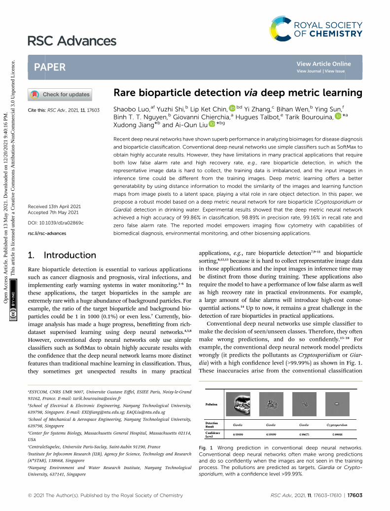
Conventional deep neural networks use simple classier tomake the decision of seen/unseen classes. Therefore, they oenmake wrong predictions, and do so condently.15–18 Forexample, the conventional deep neural network model predictswrongly (it predicts the pollutants as Cryptosporidium or Giar-dia) with a high condence level (>99.99%) as shown in Fig. 1.These inaccuracies arise from the conventional classication

Fig. 1 Wrong prediction in conventional deep neural networks.Conventional deep neural networks often make wrong predictionsand do so confidently when the images are not seen in the trainingprocess. The pollutions are predicted as targets, Giardia or Crypto-sporidium, with a confidence level >99.99%.

RSC Adv., 2021, 11, 17603–17610 | 17603

RSC Advances Paper

Ope

n A

cces

s A

rtic

le. P

ublis

hed

on 1

3 M

ay 2

021.

Dow

nloa

ded

on 1

2/20

/202

1 9:

40:1

6 PM

. T

his

artic

le is

lice

nsed

und

er a

Cre

ativ

e C

omm

ons

Attr

ibut

ion-

Non

Com

mer

cial

3.0

Unp

orte

d L

icen

ce.

View Article Online

approaches such as convolutional neural networks (CNNs) witha linear Somax classier11 (Fig. 2(a)) that limit their ability todetect novel examples.9,15,17,19,20 As a result, conventionalSomax-based approaches are not suitable for open-set rarebioparticle detection. For example, a highly accurate algorithmbased on a sophisticated densely connected neural network forbioparticle classication was developed for rare bioparticledetection,8 but it only achieved a sensitivity and specicity of77.3% and 99.5%, respectively.

Deep metric learning10 in Fig. 2(b) provides a possibledirection to improve open-set detection by learning a map fromthe input image space to an output embedding features in thelatent space. Instead of using the SoMax classier, thisapproach uses semantic similarity such as the Euclideandistance to constrain the models. It does not rely on the cross-entropy loss but proposes another class of network loss, i.e., thecontrastive loss. Thus, the sum of the output class probabilitiesis not doom to be one and this provides it a generatability.9

Generative model is essentially a metric learning problemwhereby the key is to learn a large margin distance metricwithin the latent space when the testing data are usuallydisjoint from the training dataset.

Unsupervised deep metric learning is used to learn a low-dimensional subspace and preserve useful geometrical informa-tion of the samples. On the other hand, supervised deep metriclearning is used to learn a projection from the sample space to thefeature space and measure the Euclidean metric in this featurespace to discriminate the results. The metric learning is dened tostudy a map function f with a dataset c ¼ {x, y, z,.}, wherebyf : c/ℝn is well dened mapping and d: ℝn � ℝn/ℝþ is the

Fig. 2 Deep classification vs. deep metric learning. (a) In deep clas-sification, the model only studies a boundary. (b) In deep metriclearning, the model studies a more generative representation withsimilar classes are close and the unsimilar classes are far away.

17604 | RSC Adv., 2021, 11, 17603–17610

Euclidean distance over ℝn: df(x, y) ¼ d(f(x), f(y)) ¼ kf(x) � f(y)k2 isclose to zero when x and y are similar.

The mathematical denition of Euclidean distance d(x, y)between x and y is expressed as10

dðx; yÞ ¼ kf ðxÞ � f ðyÞk2 ¼ffiffiffiffiffiffiffiffiffiffiffiffiffiffiffiffiffiffiffiffiffiffiffiffiffiffiffiffiffiffiffiffiffiffiffiffiffiffiffiffiffiffiffiffiffiffiffiffiffiffiffiffiffiffiffiffiffiðf ðxÞ � f ðyÞÞT ðf ðxÞ � f ðyÞÞ2

q(1)

where x, y ˛ c, and it is assumed that metricdðx; yÞ: c� c/ℝþ satises the following properties as

d(x, y) $ 0 (2a)

d(x, y) ¼ d(y, x) (2b)

d(x, z) # d(x, y) + d(y, z) (2c)

d(x, x) ¼ 0 (2d)

Deep metric learning is widely applied in signature veri-cation,21 face verication and recognition,22 and person re-identication.23

In this paper, a rare bioparticle detection system is demon-strated (Fig. 3), which consists of an imaging ow cytometrysystem to capture the images of all pollutants and create animage database. A deep neural network based on deep metriclearning and a decision algorithm are designed to detect rarebioparticles of Cryptosporidium and Giardia. The model lever-ages convolutional neural network to study the rich features inthe dataset and learning distinct metric by using Siamesenetwork21 and contrastive loss, which maximizes the distance ofdifferent classes and minimizes the distance of similar classes.Experimental results showed that the deep metric learningstudies good features and performs better than conventionaldeep learning, which was manifested to be a solid networkmodel for rare bioparticle detection problems.

Fig. 3 Overview of a deep metric neural network for rare bioparticledetection using an imaging flow cytometry. Water sample is processedusing (a) the imaging flow cytometry system (Amnis® ImageStream®XMk II), capturing the images of all pollutants and creating (b) an imagedatabase. (c) Deep metric neural network, and (d) decision algorithmsare used for classification and detection.

© 2021 The Author(s). Published by the Royal Society of Chemistry

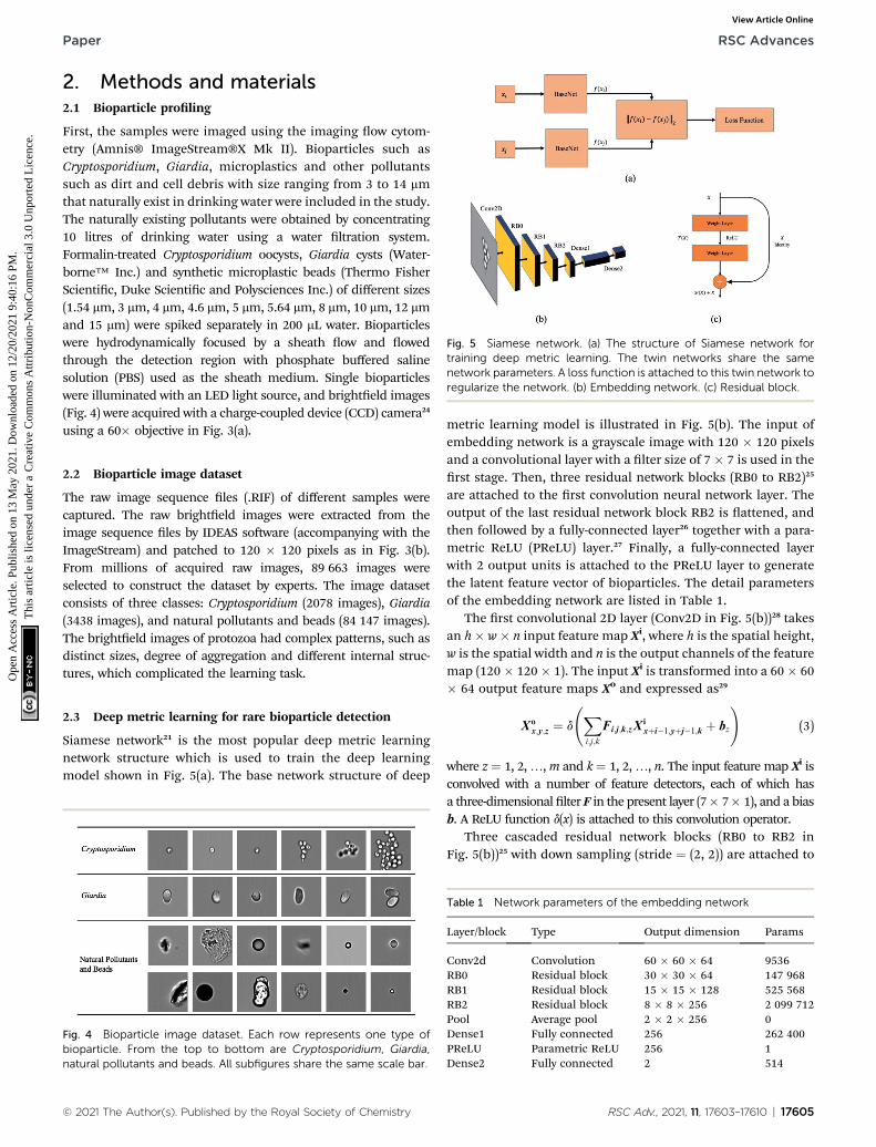
Fig. 5 Siamese network. (a) The structure of Siamese network fortraining deep metric learning. The twin networks share the samenetwork parameters. A loss function is attached to this twin network toregularize the network. (b) Embedding network. (c) Residual block.

Paper RSC Advances

Ope

n A

cces

s A

rtic

le. P

ublis

hed

on 1

3 M

ay 2

021.

Dow

nloa

ded

on 1

2/20

/202

1 9:

40:1

6 PM

. T

his

artic

le is

lice

nsed

und

er a

Cre

ativ

e C

omm

ons

Attr

ibut

ion-

Non

Com

mer

cial

3.0

Unp

orte

d L

icen

ce.

View Article Online

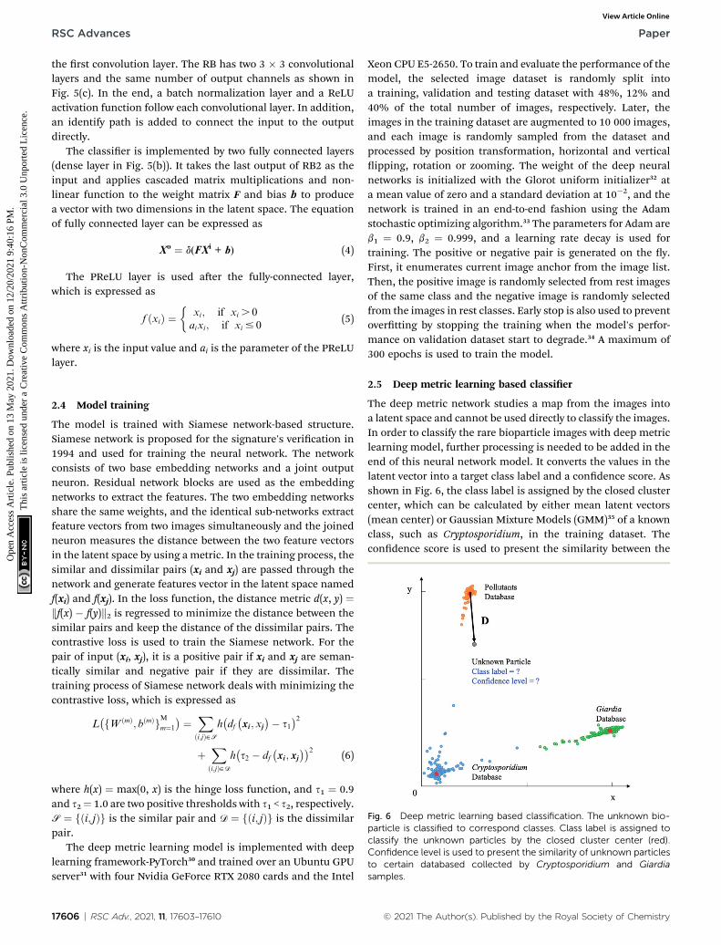
2. Methods and materials2.1 Bioparticle proling

First, the samples were imaged using the imaging ow cytom-etry (Amnis® ImageStream®X Mk II). Bioparticles such asCryptosporidium, Giardia, microplastics and other pollutantssuch as dirt and cell debris with size ranging from 3 to 14 mmthat naturally exist in drinking water were included in the study.The naturally existing pollutants were obtained by concentrating10 litres of drinking water using a water ltration system.Formalin-treated Cryptosporidium oocysts, Giardia cysts (Water-borne™ Inc.) and synthetic microplastic beads (Thermo FisherScientic, Duke Scientic and Polysciences Inc.) of different sizes(1.54 mm, 3 mm, 4 mm, 4.6 mm, 5 mm, 5.64 mm, 8 mm, 10 mm, 12 mmand 15 mm) were spiked separately in 200 mL water. Bioparticleswere hydrodynamically focused by a sheath ow and owedthrough the detection region with phosphate buffered salinesolution (PBS) used as the sheath medium. Single bioparticleswere illuminated with an LED light source, and brighteld images(Fig. 4) were acquired with a charge-coupled device (CCD) camera24

using a 60� objective in Fig. 3(a).

2.2 Bioparticle image dataset

The raw image sequence les (.RIF) of different samples werecaptured. The raw brighteld images were extracted from theimage sequence les by IDEAS soware (accompanying with theImageStream) and patched to 120 � 120 pixels as in Fig. 3(b).From millions of acquired raw images, 89 663 images wereselected to construct the dataset by experts. The image datasetconsists of three classes: Cryptosporidium (2078 images), Giardia(3438 images), and natural pollutants and beads (84 147 images).The brighteld images of protozoa had complex patterns, such asdistinct sizes, degree of aggregation and different internal struc-tures, which complicated the learning task.

2.3 Deep metric learning for rare bioparticle detection

Siamese network21 is the most popular deep metric learningnetwork structure which is used to train the deep learningmodel shown in Fig. 5(a). The base network structure of deep

Fig. 4 Bioparticle image dataset. Each row represents one type ofbioparticle. From the top to bottom are Cryptosporidium, Giardia,natural pollutants and beads. All subfigures share the same scale bar.

© 2021 The Author(s). Published by the Royal Society of Chemistry

metric learning model is illustrated in Fig. 5(b). The input ofembedding network is a grayscale image with 120 � 120 pixelsand a convolutional layer with a lter size of 7 � 7 is used in therst stage. Then, three residual network blocks (RB0 to RB2)25

are attached to the rst convolution neural network layer. Theoutput of the last residual network block RB2 is attened, andthen followed by a fully-connected layer26 together with a para-metric ReLU (PReLU) layer.27 Finally, a fully-connected layerwith 2 output units is attached to the PReLU layer to generatethe latent feature vector of bioparticles. The detail parametersof the embedding network are listed in Table 1.

The rst convolutional 2D layer (Conv2D in Fig. 5(b))28 takesan h� w� n input feature map Xi, where h is the spatial height,w is the spatial width and n is the output channels of the featuremap (120 � 120 � 1). The input Xi is transformed into a 60 � 60� 64 output feature maps Xo and expressed as29

Xox;y;z ¼ d

Xi;j;k

Fi;j;k;zXixþi�1;yþj�1;k þ bz

!(3)

where z¼ 1, 2,.,m and k¼ 1, 2,., n. The input feature map Xi isconvolved with a number of feature detectors, each of which hasa three-dimensional lter F in the present layer (7� 7� 1), and a biasb. A ReLU function d(x) is attached to this convolution operator.

Three cascaded residual network blocks (RB0 to RB2 inFig. 5(b))25 with down sampling (stride ¼ (2, 2)) are attached to

Table 1 Network parameters of the embedding network

Layer/block Type Output dimension Params

Conv2d Convolution 60 � 60 � 64 9536RB0 Residual block 30 � 30 � 64 147 968RB1 Residual block 15 � 15 � 128 525 568RB2 Residual block 8 � 8 � 256 2 099 712Pool Average pool 2 � 2 � 256 0Dense1 Fully connected 256 262 400PReLU Parametric ReLU 256 1Dense2 Fully connected 2 514

RSC Adv., 2021, 11, 17603–17610 | 17605

RSC Advances Paper

Ope

n A

cces

s A

rtic

le. P

ublis

hed

on 1

3 M

ay 2

021.

Dow

nloa

ded

on 1

2/20

/202

1 9:

40:1

6 PM

. T

his

artic

le is

lice

nsed

und

er a

Cre

ativ

e C

omm

ons

Attr

ibut

ion-

Non

Com

mer

cial

3.0

Unp

orte

d L

icen

ce.

View Article Online

the rst convolution layer. The RB has two 3 � 3 convolutionallayers and the same number of output channels as shown inFig. 5(c). In the end, a batch normalization layer and a ReLUactivation function follow each convolutional layer. In addition,an identify path is added to connect the input to the outputdirectly.

The classier is implemented by two fully connected layers(dense layer in Fig. 5(b)). It takes the last output of RB2 as theinput and applies cascaded matrix multiplications and non-linear function to the weight matrix F and bias b to producea vector with two dimensions in the latent space. The equationof fully connected layer can be expressed as

Xo ¼ d(FXi + b) (4)

The PReLU layer is used aer the fully-connected layer,which is expressed as

f ðxiÞ ¼�

xi; if xi . 0aixi; if xi # 0

(5)

where xi is the input value and ai is the parameter of the PReLUlayer.

Fig. 6 Deep metric learning based classification. The unknown bio-particle is classified to correspond classes. Class label is assigned toclassify the unknown particles by the closed cluster center (red).Confidence level is used to present the similarity of unknown particlesto certain databased collected by Cryptosporidium and Giardiasamples.

2.4 Model training

The model is trained with Siamese network-based structure.Siamese network is proposed for the signature's verication in1994 and used for training the neural network. The networkconsists of two base embedding networks and a joint outputneuron. Residual network blocks are used as the embeddingnetworks to extract the features. The two embedding networksshare the same weights, and the identical sub-networks extractfeature vectors from two images simultaneously and the joinedneuron measures the distance between the two feature vectorsin the latent space by using ametric. In the training process, thesimilar and dissimilar pairs (xi and xj) are passed through thenetwork and generate features vector in the latent space namedf(xi) and f(xj). In the loss function, the distance metric d(x, y) ¼kf(x) � f(y)k2 is regressed to minimize the distance between thesimilar pairs and keep the distance of the dissimilar pairs. Thecontrastive loss is used to train the Siamese network. For thepair of input (xi, xj), it is a positive pair if xi and xj are seman-tically similar and negative pair if they are dissimilar. Thetraining process of Siamese network deals with minimizing thecontrastive loss, which is expressed as

L�fW ðmÞ; bðmÞgMm¼1

� ¼ Xði;jÞ˛S

h�df�xi ; xj

�� s1�2

þXði;jÞ˛D

h�s2 � df

�xi ; xj

��2(6)

where h(x) ¼ max(0, x) is the hinge loss function, and s1 ¼ 0.9and s2¼ 1.0 are two positive thresholds with s1 < s2, respectively.S ¼ fði; jÞg is the similar pair and D ¼ fði; jÞg is the dissimilarpair.

The deep metric learning model is implemented with deeplearning framework-PyTorch30 and trained over an Ubuntu GPUserver31 with four Nvidia GeForce RTX 2080 cards and the Intel

17606 | RSC Adv., 2021, 11, 17603–17610

Xeon CPU E5-2650. To train and evaluate the performance of themodel, the selected image dataset is randomly split intoa training, validation and testing dataset with 48%, 12% and40% of the total number of images, respectively. Later, theimages in the training dataset are augmented to 10 000 images,and each image is randomly sampled from the dataset andprocessed by position transformation, horizontal and verticalipping, rotation or zooming. The weight of the deep neuralnetworks is initialized with the Glorot uniform initializer32 ata mean value of zero and a standard deviation at 10�2, and thenetwork is trained in an end-to-end fashion using the Adamstochastic optimizing algorithm.33 The parameters for Adam areb1 ¼ 0.9, b2 ¼ 0.999, and a learning rate decay is used fortraining. The positive or negative pair is generated on the y.First, it enumerates current image anchor from the image list.Then, the positive image is randomly selected from rest imagesof the same class and the negative image is randomly selectedfrom the images in rest classes. Early stop is also used to preventovertting by stopping the training when the model's perfor-mance on validation dataset start to degrade.34 A maximum of300 epochs is used to train the model.

2.5 Deep metric learning based classier

The deep metric network studies a map from the images intoa latent space and cannot be used directly to classify the images.In order to classify the rare bioparticle images with deep metriclearning model, further processing is needed to be added in theend of this neural network model. It converts the values in thelatent vector into a target class label and a condence score. Asshown in Fig. 6, the class label is assigned by the closed clustercenter, which can be calculated by either mean latent vectors(mean center) or Gaussian Mixture Models (GMM)35 of a knownclass, such as Cryptosporidium, in the training dataset. Thecondence score is used to present the similarity between the

© 2021 The Author(s). Published by the Royal Society of Chemistry

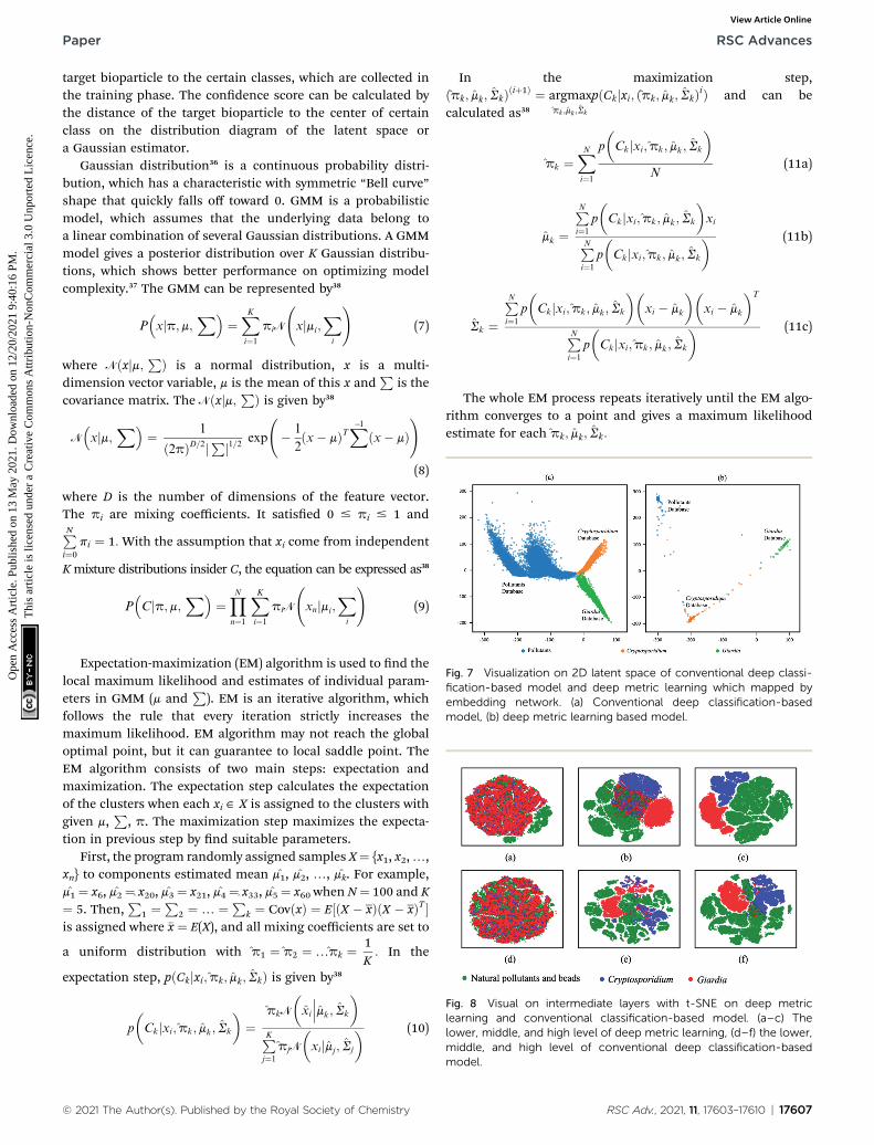
Fig. 7 Visualization on 2D latent space of conventional deep classi-fication-based model and deep metric learning which mapped byembedding network. (a) Conventional deep classification-basedmodel, (b) deep metric learning based model.

Fig. 8 Visual on intermediate layers with t-SNE on deep metriclearning and conventional classification-based model. (a–c) Thelower, middle, and high level of deep metric learning, (d–f) the lower,middle, and high level of conventional deep classification-basedmodel.

Paper RSC Advances

Ope

n A

cces

s A

rtic

le. P

ublis

hed

on 1

3 M

ay 2

021.

Dow

nloa

ded

on 1

2/20

/202

1 9:

40:1

6 PM

. T

his

artic

le is

lice

nsed

und

er a

Cre

ativ

e C

omm

ons

Attr

ibut

ion-

Non

Com

mer

cial

3.0

Unp

orte

d L

icen

ce.

View Article Online

target bioparticle to the certain classes, which are collected inthe training phase. The condence score can be calculated bythe distance of the target bioparticle to the center of certainclass on the distribution diagram of the latent space ora Gaussian estimator.

Gaussian distribution36 is a continuous probability distri-bution, which has a characteristic with symmetric “Bell curve”shape that quickly falls off toward 0. GMM is a probabilisticmodel, which assumes that the underlying data belong toa linear combination of several Gaussian distributions. A GMMmodel gives a posterior distribution over K Gaussian distribu-tions, which shows better performance on optimizing modelcomplexity.37 The GMM can be represented by38

P�xjp;m;

X�¼XKi¼1

piN

xjmi;

Xi

!(7)

where N ðxjm; PÞ is a normal distribution, x is a multi-dimension vector variable, m is the mean of this x and

Pis the

covariance matrix. The N ðxjm; PÞ is given by38

N�xjm;

X�¼ 1

ð2pÞD=2jPj1=2exp

� 1

2ðx� mÞT

X�1ðx� mÞ

!

(8)

where D is the number of dimensions of the feature vector.The pi are mixing coefficients. It satised 0 # pi # 1 andPNi¼0

pi ¼ 1: With the assumption that xi come from independent

Kmixture distributions insider C, the equation can be expressed as38

P�Cjp;m;

X�¼YNn¼1

XKi¼1

piN

xnjmi;

Xi

!(9)

Expectation-maximization (EM) algorithm is used to nd thelocal maximum likelihood and estimates of individual param-eters in GMM (m and

P). EM is an iterative algorithm, which

follows the rule that every iteration strictly increases themaximum likelihood. EM algorithm may not reach the globaloptimal point, but it can guarantee to local saddle point. TheEM algorithm consists of two main steps: expectation andmaximization. The expectation step calculates the expectationof the clusters when each xi ˛ X is assigned to the clusters withgiven m,

P, p. The maximization step maximizes the expecta-

tion in previous step by nd suitable parameters.First, the program randomly assigned samples X¼ {x1, x2,.,

xn} to components estimated mean m1, m2, ., mk. For example,m1 ¼ x6, m2 ¼ x20, m3¼ x21, m4¼ x33, m5¼ x60 when N¼ 100 and K¼ 5. Then,

P1 ¼

P2 ¼ . ¼ Pk ¼ CovðxÞ ¼ E½ðX � xÞðX � xÞT �

is assigned where �x ¼ E(X), and all mixing coefficients are set to

a uniform distribution with p1 ¼ p2 ¼ .pk ¼ 1K: In the

expectation step, pðCkjxi ;pk; mk; SkÞ is given by38

p

�Ckjxi ;pk; mk; Sk

¼

pkN�xi

mk; Sk

PKj¼1

pjN�xijmj; Sj

(10)

© 2021 The Author(s). Published by the Royal Society of Chemistry

In the maximization step,ðpk; mk; SkÞðiþ1Þ ¼ argmax

pk ;mk ;Sk

pðCkjxi; ðpk; mk; SkÞiÞ and can becalculated as38

pk ¼XNi¼1

p

�Ckjxi ;pk; mk; Sk

N

(11a)

mk ¼PNi¼1

p

�Ckjxi ;pk; mk; Sk

xi

PNi¼1

p

�Ckjxi ;pk; mk; Sk

(11b)

Sk ¼PNi¼1

p

�Ckjxi ;pk; mk; Sk

�xi � mk

�xi � mk

T

PNi¼1

p

�Ckjxi ;pk; mk; Sk

(11c)

The whole EM process repeats iteratively until the EM algo-rithm converges to a point and gives a maximum likelihoodestimate for each pk; mk; Sk:

RSC Adv., 2021, 11, 17603–17610 | 17607

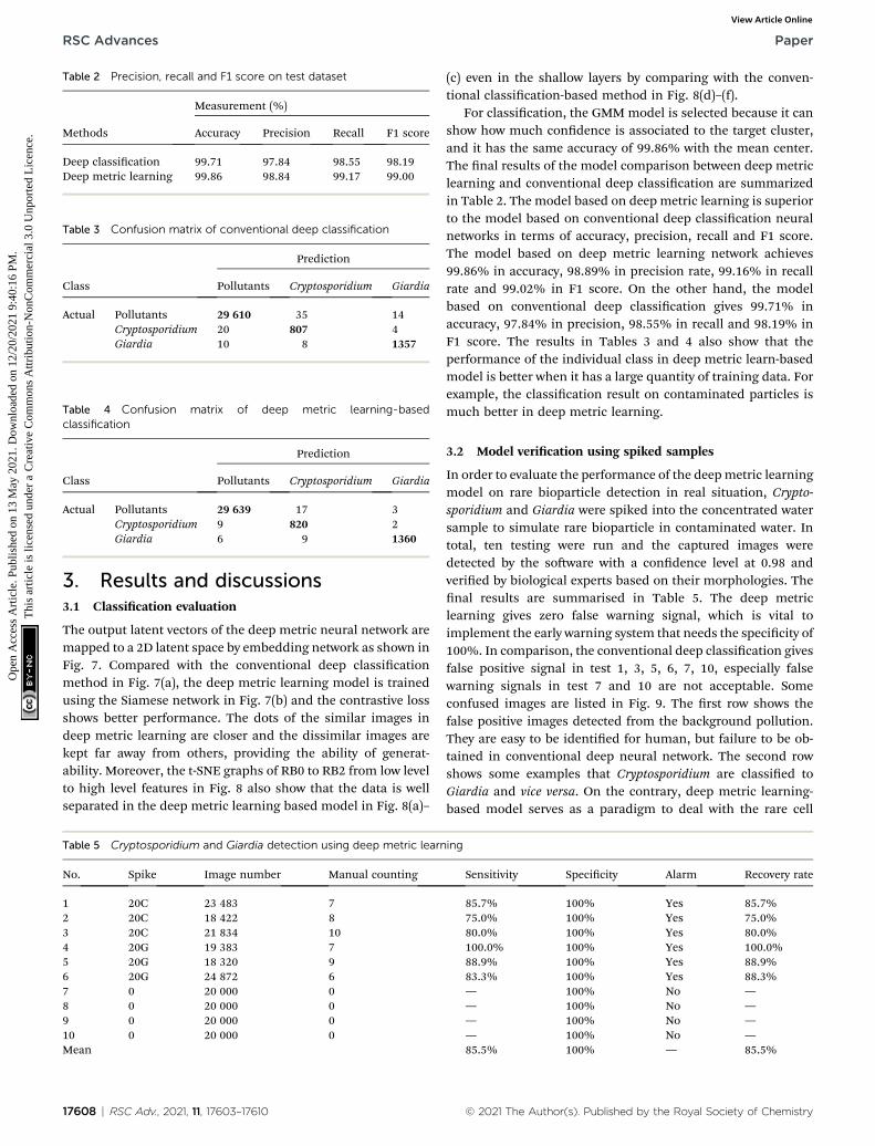
Table 2 Precision, recall and F1 score on test dataset

Methods

Measurement (%)

Accuracy Precision Recall F1 score

Deep classication 99.71 97.84 98.55 98.19Deep metric learning 99.86 98.84 99.17 99.00

Table 3 Confusion matrix of conventional deep classification

Class

Prediction

Pollutants Cryptosporidium Giardia

Actual Pollutants 29 610 35 14Cryptosporidium 20 807 4Giardia 10 8 1357

Table 4 Confusion matrix of deep metric learning-basedclassification

Class

Prediction

Pollutants Cryptosporidium Giardia

Actual Pollutants 29 639 17 3Cryptosporidium 9 820 2Giardia 6 9 1360

RSC Advances Paper

Ope

n A

cces

s A

rtic

le. P

ublis

hed

on 1

3 M

ay 2

021.

Dow

nloa

ded

on 1

2/20

/202

1 9:

40:1

6 PM

. T

his

artic

le is

lice

nsed

und

er a

Cre

ativ

e C

omm

ons

Attr

ibut

ion-

Non

Com

mer

cial

3.0

Unp

orte

d L

icen

ce.

View Article Online

3. Results and discussions3.1 Classication evaluation

The output latent vectors of the deep metric neural network aremapped to a 2D latent space by embedding network as shown inFig. 7. Compared with the conventional deep classicationmethod in Fig. 7(a), the deep metric learning model is trainedusing the Siamese network in Fig. 7(b) and the contrastive lossshows better performance. The dots of the similar images indeep metric learning are closer and the dissimilar images arekept far away from others, providing the ability of generat-ability. Moreover, the t-SNE graphs of RB0 to RB2 from low levelto high level features in Fig. 8 also show that the data is wellseparated in the deep metric learning based model in Fig. 8(a)–

Table 5 Cryptosporidium and Giardia detection using deep metric learn

No. Spike Image number Manual counting

1 20C 23 483 72 20C 18 422 83 20C 21 834 104 20G 19 383 75 20G 18 320 96 20G 24 872 67 0 20 000 08 0 20 000 09 0 20 000 010 0 20 000 0Mean

17608 | RSC Adv., 2021, 11, 17603–17610

(c) even in the shallow layers by comparing with the conven-tional classication-based method in Fig. 8(d)–(f).

For classication, the GMM model is selected because it canshow how much condence is associated to the target cluster,and it has the same accuracy of 99.86% with the mean center.The nal results of the model comparison between deep metriclearning and conventional deep classication are summarizedin Table 2. The model based on deep metric learning is superiorto the model based on conventional deep classication neuralnetworks in terms of accuracy, precision, recall and F1 score.The model based on deep metric learning network achieves99.86% in accuracy, 98.89% in precision rate, 99.16% in recallrate and 99.02% in F1 score. On the other hand, the modelbased on conventional deep classication gives 99.71% inaccuracy, 97.84% in precision, 98.55% in recall and 98.19% inF1 score. The results in Tables 3 and 4 also show that theperformance of the individual class in deep metric learn-basedmodel is better when it has a large quantity of training data. Forexample, the classication result on contaminated particles ismuch better in deep metric learning.

3.2 Model verication using spiked samples

In order to evaluate the performance of the deepmetric learningmodel on rare bioparticle detection in real situation, Crypto-sporidium and Giardia were spiked into the concentrated watersample to simulate rare bioparticle in contaminated water. Intotal, ten testing were run and the captured images weredetected by the soware with a condence level at 0.98 andveried by biological experts based on their morphologies. Thenal results are summarised in Table 5. The deep metriclearning gives zero false warning signal, which is vital toimplement the early warning system that needs the specicity of100%. In comparison, the conventional deep classication givesfalse positive signal in test 1, 3, 5, 6, 7, 10, especially falsewarning signals in test 7 and 10 are not acceptable. Someconfused images are listed in Fig. 9. The rst row shows thefalse positive images detected from the background pollution.They are easy to be identied for human, but failure to be ob-tained in conventional deep neural network. The second rowshows some examples that Cryptosporidium are classied toGiardia and vice versa. On the contrary, deep metric learning-based model serves as a paradigm to deal with the rare cell

ing

Sensitivity Specicity Alarm Recovery rate

85.7% 100% Yes 85.7%75.0% 100% Yes 75.0%80.0% 100% Yes 80.0%100.0% 100% Yes 100.0%88.9% 100% Yes 88.9%83.3% 100% Yes 88.3%— 100% No —— 100% No —— 100% No —— 100% No —85.5% 100% — 85.5%

© 2021 The Author(s). Published by the Royal Society of Chemistry

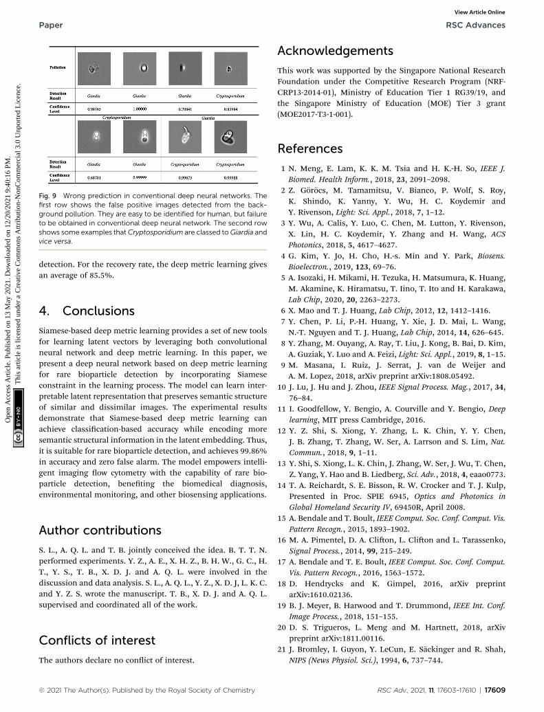
Fig. 9 Wrong prediction in conventional deep neural networks. Thefirst row shows the false positive images detected from the back-ground pollution. They are easy to be identified for human, but failureto be obtained in conventional deep neural network. The second rowshows some examples thatCryptosporidium are classed toGiardia andvice versa.

Paper RSC Advances

Ope

n A

cces

s A

rtic

le. P

ublis

hed

on 1

3 M

ay 2

021.

Dow

nloa

ded

on 1

2/20

/202

1 9:

40:1

6 PM

. T

his

artic

le is

lice

nsed

und

er a

Cre

ativ

e C

omm

ons

Attr

ibut

ion-

Non

Com

mer

cial

3.0

Unp

orte

d L

icen

ce.

View Article Online

detection. For the recovery rate, the deep metric learning givesan average of 85.5%.

4. Conclusions

Siamese-based deep metric learning provides a set of new toolsfor learning latent vectors by leveraging both convolutionalneural network and deep metric learning. In this paper, wepresent a deep neural network based on deep metric learningfor rare bioparticle detection by incorporating Siameseconstraint in the learning process. The model can learn inter-pretable latent representation that preserves semantic structureof similar and dissimilar images. The experimental resultsdemonstrate that Siamese-based deep metric learning canachieve classication-based accuracy while encoding moresemantic structural information in the latent embedding. Thus,it is suitable for rare bioparticle detection, and achieves 99.86%in accuracy and zero false alarm. The model empowers intelli-gent imaging ow cytometry with the capability of rare bio-particle detection, beneting the biomedical diagnosis,environmental monitoring, and other biosensing applications.

Author contributions

S. L., A. Q. L. and T. B. jointly conceived the idea. B. T. T. N.performed experiments. Y. Z., A. E., X. H. Z., B. H. W., G. C., H.T., Y. S., T. B., X. D. J. and A. Q. L. were involved in thediscussion and data analysis. S. L., A. Q. L., Y. Z., X. D. J, L. K. C.and Y. Z. S. wrote the manuscript. T. B., X. D. J. and A. Q. L.supervised and coordinated all of the work.

Conflicts of interest

The authors declare no conict of interest.

© 2021 The Author(s). Published by the Royal Society of Chemistry

Acknowledgements

This work was supported by the Singapore National ResearchFoundation under the Competitive Research Program (NRF-CRP13-2014-01), Ministry of Education Tier 1 RG39/19, andthe Singapore Ministry of Education (MOE) Tier 3 grant(MOE2017-T3-1-001).

References

1 N. Meng, E. Lam, K. K. M. Tsia and H. K.-H. So, IEEE J.Biomed. Health Inform., 2018, 23, 2091–2098.

2 Z. Gorocs, M. Tamamitsu, V. Bianco, P. Wolf, S. Roy,K. Shindo, K. Yanny, Y. Wu, H. C. Koydemir andY. Rivenson, Light: Sci. Appl., 2018, 7, 1–12.

3 Y. Wu, A. Calis, Y. Luo, C. Chen, M. Lutton, Y. Rivenson,X. Lin, H. C. Koydemir, Y. Zhang and H. Wang, ACSPhotonics, 2018, 5, 4617–4627.

4 G. Kim, Y. Jo, H. Cho, H.-s. Min and Y. Park, Biosens.Bioelectron., 2019, 123, 69–76.

5 A. Isozaki, H. Mikami, H. Tezuka, H. Matsumura, K. Huang,M. Akamine, K. Hiramatsu, T. Iino, T. Ito and H. Karakawa,Lab Chip, 2020, 20, 2263–2273.

6 X. Mao and T. J. Huang, Lab Chip, 2012, 12, 1412–1416.7 Y. Chen, P. Li, P.-H. Huang, Y. Xie, J. D. Mai, L. Wang,N.-T. Nguyen and T. J. Huang, Lab Chip, 2014, 14, 626–645.

8 Y. Zhang, M. Ouyang, A. Ray, T. Liu, J. Kong, B. Bai, D. Kim,A. Guziak, Y. Luo and A. Feizi, Light: Sci. Appl., 2019, 8, 1–15.

9 M. Masana, I. Ruiz, J. Serrat, J. van de Weijer andA. M. Lopez, 2018, arXiv preprint arXiv:1808.05492.

10 J. Lu, J. Hu and J. Zhou, IEEE Signal Process. Mag., 2017, 34,76–84.

11 I. Goodfellow, Y. Bengio, A. Courville and Y. Bengio, Deeplearning, MIT press Cambridge, 2016.

12 Y. Z. Shi, S. Xiong, Y. Zhang, L. K. Chin, Y. Y. Chen,J. B. Zhang, T. Zhang, W. Ser, A. Larrson and S. Lim, Nat.Commun., 2018, 9, 1–11.

13 Y. Shi, S. Xiong, L. K. Chin, J. Zhang, W. Ser, J. Wu, T. Chen,Z. Yang, Y. Hao and B. Liedberg, Sci. Adv., 2018, 4, eaao0773.

14 T. A. Reichardt, S. E. Bisson, R. W. Crocker and T. J. Kulp,Presented in Proc. SPIE 6945, Optics and Photonics inGlobal Homeland Security IV, 69450R, April 2008.

15 A. Bendale and T. Boult, IEEE Comput. Soc. Conf. Comput. Vis.Pattern Recogn., 2015, 1893–1902.

16 M. A. Pimentel, D. A. Clion, L. Clion and L. Tarassenko,Signal Process., 2014, 99, 215–249.

17 A. Bendale and T. E. Boult, IEEE Comput. Soc. Conf. Comput.Vis. Pattern Recogn., 2016, 1563–1572.

18 D. Hendrycks and K. Gimpel, 2016, arXiv preprintarXiv:1610.02136.

19 B. J. Meyer, B. Harwood and T. Drummond, IEEE Int. Conf.Image Process., 2018, 151–155.

20 D. S. Trigueros, L. Meng and M. Hartnett, 2018, arXivpreprint arXiv:1811.00116.

21 J. Bromley, I. Guyon, Y. LeCun, E. Sackinger and R. Shah,NIPS (News Physiol. Sci.), 1994, 6, 737–744.

RSC Adv., 2021, 11, 17603–17610 | 17609

RSC Advances Paper

Ope

n A

cces

s A

rtic

le. P

ublis

hed

on 1

3 M

ay 2

021.

Dow

nloa

ded

on 1

2/20

/202

1 9:

40:1

6 PM

. T

his

artic

le is

lice

nsed

und

er a

Cre

ativ

e C

omm

ons

Attr

ibut

ion-

Non

Com

mer

cial

3.0

Unp

orte

d L

icen

ce.

View Article Online

22 Y. Taigman, M. Yang, M. A. Ranzato and L. Wolf, IEEEComput. Soc. Conf. Comput. Vis. Pattern Recogn., 2014,1701–1708.

23 R. R. Varior, M. Haloi and G. Wang, ECCV, 2016.24 E. R. Fossum and D. B. Hondongwa, IEEE J. Electron Devices

Soc., 2014, 2(3), 33–43.25 K. He, X. Zhang, S. Ren and J. Sun, IEEE Comput. Soc. Conf.

Comput. Vis. Pattern Recogn., 2016, 770–778.26 Y. LeCun, Y. Bengio and G. Hinton, Nature, 2015, 521, 436–

444.27 K. He, X. Zhang, S. Ren and J. Sun, IEEE International

Conference on Computer Vision, 2015, 1026–1034.28 Y. LeCun, B. E. Boser, J. S. Denker, D. Henderson,

R. E. Howard, W. E. Hubbard and L. D. Jackel, NIPS (NewsPhysiol. Sci.), 1990, 396–404.

29 A. G. Howard, M. Zhu, B. Chen, D. Kalenichenko, W. Wang,T. Weyand, M. Andreetto and H. Adam, 2017, arXiv preprintarXiv:1704.04861.

17610 | RSC Adv., 2021, 11, 17603–17610

30 A. Paszke, S. Gross, F. Massa, A. Lerer, J. Bradbury,G. Chanan, T. Killeen, Z. Lin, N. Gimelshein and L. Antiga,NIPS (News Physiol. Sci.), 2019, 32.

31 M. Hodak, M. Gorkovenko and A. Dholakia, Towards powerefficiency in deep learning on data center hardware, in 2019IEEE International Conference on Big Data (Big Data), IEEE,2019, pp. 1814–1820.

32 X. Glorot and Y. Bengio, ICAIS, 2010.33 D. P. Kingma and J. Ba, 2014, arXiv preprint arXiv:1412.6980.34 R. Caruana, S. Lawrence and C. L. Giles, NIPS (News Physiol.

Sci.), 2001, 402–408.35 D. A. Reynolds, Encyclopedia of Biometrics, 2009, p. 741.36 W. M. Mendenhall and T. L. Sincich, Statistics for Engineering

and the Sciences, CRC Press, 2016.37 A. Corduneanu and C. M. Bishop, ICAIS, 2001.38 D. A. Forsyth and J. Ponce, Computer vision: a modern

approach, Pearson, 2012.

© 2021 The Author(s). Published by the Royal Society of Chemistry